Modave Lectures

Aspects of two-dimensional Conformal FieldTheory

Stephane Detournay♥,1

♥Mecanique et GravitationUniversite de Mons-Hainaut, 20 Place du Parc

7000 Mons, Belgium

Abstract

These notes constitute the write-up of a four hour lecture given at the First Modave SummerSchool on Mathematical Physics, held in Modave, 19-25 june 2005. It is intended to introducebasic tools of conformal field theory in two dimensions using as guideline the conformal Wardidentities. Comments are welcome!

1E-mail : Stephane.Detournay@umh.ac.be, ”Chercheur FRIA”

Contents

1 Conformal transformations in two dimensions 2

2 Conformal Ward identities in two dimensions : part I 72.1 Preliminaries . . . . . . . . . . . . . . . . . . . . . . . . . . . . . . . . . . . . . . . . 72.2 A derivation of the conformal Ward identities . . . . . . . . . . . . . . . . . . . . . . 8

3 Operator product expansion and conformal transformation of fields 16

4 Operator formalism 194.1 Radial quantization . . . . . . . . . . . . . . . . . . . . . . . . . . . . . . . . . . . . . 194.2 Mode expansions and Virasoro algebra . . . . . . . . . . . . . . . . . . . . . . . . . . 244.3 The Hilbert space and representations of the Virasoro algebra . . . . . . . . . . . . . 264.4 Ward identities strike back : global Ward identities . . . . . . . . . . . . . . . . . . . 294.5 Descendant fields . . . . . . . . . . . . . . . . . . . . . . . . . . . . . . . . . . . . . . 314.6 Operator algebra . . . . . . . . . . . . . . . . . . . . . . . . . . . . . . . . . . . . . . 344.7 Ward identities: final chapter . . . . . . . . . . . . . . . . . . . . . . . . . . . . . . . 364.8 A short story on normal ordering . . . . . . . . . . . . . . . . . . . . . . . . . . . . . 37

5 The free boson 39

6 Exercises 416.1 Operator formalism . . . . . . . . . . . . . . . . . . . . . . . . . . . . . . . . . . . . . 416.2 Free boson . . . . . . . . . . . . . . . . . . . . . . . . . . . . . . . . . . . . . . . . . . 416.3 Ghost system . . . . . . . . . . . . . . . . . . . . . . . . . . . . . . . . . . . . . . . . 42

Acknowledgments 43

Appendix A : Another derivation of the conformal Ward identities 43

Bibliography 46

1 Conformal transformations in two dimensions

Consider flat space-time in d dimensions, that is, Rd endowed with a flat metric gµν (which willbe taken euclidian or lorentzian) and coordinates xµ, µ = 0, · · · , d − 1. First recall that Poincaretransformations are the set of transformations

xµ → x′µ(x) , µ = 0, · · · , d− 1 (1)

leaving the components of the flat metric (with lorentzian signature) unchanged :

gµν→g′µν(x′(x))

!= gµν(x) . (2)

This statement can also be expressed from the ”active” point of view by demanding that the squared”Minkowskian norm” ds2 of a vector with components dxµ be preserved under (1) :

ds2 = gµν dxµdxν → ds′2 = gµν dx′µdx′ν != ds2 , (3)

2

that is

gµν∂x′µ

∂xα

∂x′ν

∂xβ= gαβ . (4)

Conformal transformations are defined as the set of transformations (1) leaving the components ofthe metric tensor invariant up to a scale :

gµν→g′µν(x′(x)) = Λ(x)gµν . (5)

Condition (5) expresses that the scalar product of basis vectors of the tangent space is conservedonly up to a local scale factor (possibly depending on the point). In particular, angles are preservedby conformal transformations. Equivalently, conformal transformations are such that

ds2 → ds′2 != Λ−1(x)ds2 . (6)

Let us focus on the two-dimensional case. We will be working with an euclidian metric, such thatthe line element is (dx1)2 + (dx2)2. We introduce complex coordinates

z = x1 + ix2 and z = x1 − ix2 , (7)

in which the metric reads ds2 = dzdz. Notice it is only in 2 dimensions that the metric in complexcoordinates factorizes in dz and dz. Consequently, any change of coordinates

z→f(z)4= z + α(z) , z→f(z)

4= z + α(z) (8)

with f and f depending only upon z and z respectively2 will satisfy (6), because

ds2→ds′2 =

(df

dz

)(df

dz

)ds2 . (9)

Actually, these are the only conformal transformations in two dimensions. To verify this, onemay consider infinitesimal transformations x′µ = xµ + εµ(x) in (5), for infinitesimal εµ(x). With

g′µν

4= gµν + f(x)gµν , one gets, to first order in εµ(x) :

∂µεν + ∂νεµ = −f(x)gµν . (10)

By taking the trace of (10), one determines f(x), so that we get

∂µεν + ∂νεµ =2

d(∂αεα)gµν , (11)

which are called conformal Killing equations. Their solution, in two dimensions, expresses that

εz(z, z) = εz(z)4= ε(z) and εz(z, z) = εz(z)

4= ε(z), see [3] for a detailed computation.

Now, suppose α(z) in (8) admits a Laurent expansion around say z = 0 (we only consider the”holomorphic” sector) :

α(z) =+∞∑

n=−∞αnzn+1 . (12)

2It is a common abuse of language to call f(z) (resp. f(z)) a holomorphic (resp. anti-holomorphic) function, becauseit may in general possess singularities. One usually restricts to meromorphic functions, i.e. functions admitting a setof isolated poles

3

On functions (scalar fields) depending only upon one coordinate (say z), the mappings (8) aregenerated by differential operators. Indeed, by considering a transformation of the form x→x′,φ(x)→φ′(x′), the variation of a field is defined as :

δφ(x) = φ′(x)− φ(x)4= ωaGaφ(x) , (13)

where {ωa} is a set of infinitesimal parameters, and Ga are the symmetry generators3. By consideringan infinitesimal version of (8), the effect on a function f(z) is

δf(z) = −α(z)∂zf(z) =∑

n

αnlnf(z) , (14)

where we used (12) with infinitesimal parameters αn, and defined the generators

ln = −zn+1∂z . (15)

They satisfy the following commutation relation

[ln, lm] = (n−m)ln+m , (16)

with analogous definition and commutation relations for the ln’s. The infinite Lie algebra defined by(16) is known as the Witt algebra. Notice that the infinitesimal transformations resulting from (15)are the most general that are analytic (or holomorphic, in strict sense) near the point z = 0. Theymay introduce singularities at z = 0, but not branch cuts4.An important subset of the transformations (8) consists in transformations defining invertible map-pings globally defined on C ∪ {∞}, that is, the complex plane plus a point at infinity. This spaceis called the Riemann sphere, as it may be compactified (through stereographic projection) to thetwo-dimensional sphere S2. These transformations are called global conformal transformations.To determine them, a first argument is based on the form (15) of the generators. Clearly ln isnon-singular at z = 0 if n ≥ −1. To investigate the behavior at ∞, consider the conformal mapz→z′ = 1

z. Under this transformation, the generator ln transforms to

−zn+1∂z−→− z′−(n+1)

(∂z′

∂z

)∂z′ = z′(1−n)∂z′ . (17)

This operator is non-singular at z′ = 0 if n ≤ 1. The generators (15) are thus defined everywhere onthe Riemann sphere if −1 ≤ n ≤ 1.Let us see to what kind of transformations they correspond. For n = −1, the infinitesimal transfor-mation is

z→z′ = z + δA , (18)

where the infinitesimal parameter α−1 is supposed to arise from the variation of a finite complexparameter A. The finite transformation follows from a trivial integration :

dz

dA= 1 ⇒

z′∫

z

dw =

A∫

0

dA ⇒ z′ = z + A . (19)

3As an example, for translations, the infinitesimal parameters are ωµ, defined by x′µ = xµ + ωµ and φ′(x′) = φ(x),so that Gµ = −∂µ

4to admit a Laurent expansion around z0, a function must be analytic in a crown centered at z0. If the functionhas a branch cut at z0 (like for instance log z at z = 0), then one cannot ”close a contour” around z0 and the Laurentexpansion cannot be defined

4

Recalling the definition of z and going back to the original coordinates x1 and x2, this correspondsto

x1→x1 + Re(A) , x2→x2 + Im(A) , (20)

and hence to translations : xµ→xµ + aµ. For n = 0, one finds, with α0 = δT :

dz

dT= z ⇒

z′∫

z

dw

w=

T∫

0

dT ⇒ z′ = Bz , B = eT . (21)

Let us consider two cases : B = eiθ and B = λ. With the first one, we find that the effect on thecoordinates (x1, x2) is

xµ→Λµν xν , Λ ∈ SO(2) , (22)

thus corresponding to rotations. At this point, we just found the (euclidian) Poincare group in twodimensions, which was expected to be a subgroup of the conformal group. With B = λ, we find that

xµ→λxµ , (23)

corresponding to dilations. Finally, for n = 1, we have

dz

z2= −D ⇒z′ =

z

1 + Dz. (24)

This transformation is called special conformal transformation (SCT), and can be seen as the com-bination of an inversion, a translation and an inversion (notice that inversions are conformal, eventhough they do not have an infinitesimal form).By combining (19),(21) and (24), one obtains the so-called global conformal transformations in twodimensions :

z′ =Bz + A

1 + D(Bz + A)=

Bz + A

(1 + BD) + BDz, (25)

whose general form is

z′ =az + b

cz + d. (26)

Notice that (26) has 4 complex parameters, while (25) has only 3. The excessive parameter is notrelevant, since we could divide numerator and denominator of (26) by d. It is however common touse this parametrization for the two-dimensional global (or finite) conformal group, with additionalcondition

det

(a bc d

)= 1 , (27)

which leaves us with 3 complex parameters. The parametrization (26) is very convenient becausesuccessive transformations correspond to the product of the corresponding matrices. Indeed, it canbe checked, by looking at successive transformations of the form

z1 =a1z + b1

c1z + d1

, z2 =a2z1 + b2

c2z1 + d2

, (28)

that the resulting transformation is

z2 =a′z + b′

c′z + d′, (29)

5

where the parameters a′,b′,c′ and d′ are given by(

a′ b′

c′ d′

)=

(a2 b2

c2 d2

)(a1 b1

c1 d1

). (30)

This establishes that the global conformal group in two dimensions is equivalent to Sl(2,C)/Z2, thequotient coming from the fact that A and −A ∈ Sl(2,C)/Z2 correspond to the same conformaltransformation5.At this level, it seems interesting to make a point about the status of the pair of variables (z, z). Itis customary to consider (x1, x2) as a point in C2, so that (7) is a mere change of coordinates , zbeing not the complex conjugate of z but rather a distinct complex coordinate. This constitutes aconvenient simplification in some situations, where one could for instance completely forget aboutthe z (sometimes called anti-holomorphic) sector and focus on the z (holomorphic) sector, becauseboth sectors are regarded as independent. The global conformal transformations would then be givenby

z→az + b

cz + d, z→ az + b

cz + d, (31)

with 8 complex parameters subject to the constraints ad−bc = 1 and ad− bc = 1, thus correspondingto the group Sl(2,C)/Z2 × Sl(2,C)/Z2. In the complex plane C2 parameterized by (z, z), the surfacewhere z = z∗ will be called the real surface, because it corresponds to (x1, x2) ∈ R2, i.e. to thephysical space. Furthermore, conformal transformations send points from the real surface on itself ifthe condition

f ∗(z) = f(z) (32)

is satisfied. Obviously, when restricted to the real surface the global conformal group reduces toSl(2,C)/Z2.Note that in obtaining (26), we assumed that the parameters of the transformations, α−1, α0, α1,are complex, and we forgot about the z dependance (assuming we are on the real surface). Anequivalent approach used in literature consists in keeping the z dependance, and then restrict thetransformations

z→z +∑

n

αnzn+1 , z→z +∑

n

αnzn+1, (33)

with real parameters αn and αn to the real surface z = z∗. The transformations preserving thereal surface (z = z∗⇒z′ = z

′∗) are generated by (ln + ln) and i(ln − ln). The global conformalgroup is thus generated by the 6 generators obtained by taking n = −1, 0, 1, which can be seento satisfy the commutation relations of the so(1, 3) real Lie algebra. It can indeed by checked

that ∂14= ∂x1 = −(l1 + l1), ∂2 = i(l1 − l1) (translations), x2∂2 − x2∂1 = −(l0 − l0) (rotations),

x1∂1 + x2∂2 = −(l0 + l0) (dilations), the remaining two corresponding to SCT.Another way of finding the form of the global conformal transformations consists in looking at thefinite transformations (8). To describe a bijective map on the Riemann sphere, the function f(z)should not have any branch point nor any essential singularity. Indeed, around a branch point themap is not uniquely defined6, whereas the image of a small neighborhood of an essential singularity

5One recognizes easily in (26) the different transformations : translations, z′ = z + b for a = d = 1 and c = 0,rotations, z′ = eiθz for c = b = 0, a = 1

d = eiθ/2, dilations, z′ = eλz for c = b = 0, a = 1d = eλ/2 and SCT, z′ = z

1+cz ,for a = d = 1, b = 0

6Consider log z = ln ρ + iϕ, for z = ρeiϕ. If one adds 2π to ϕ, this doesn’t change z, but the imaginary part oflog z gets modified, showing that log z is a ”multivalued function” having distinct branches

6

under f is dense in C (Weierstrass’ theorem). Thus f is not invertible in these cases, and the onlyacceptable singularities are poles. Then, f can be written as a ratio of polynomials without commonzeros7

f(z) =P (z)

Q(z). (34)

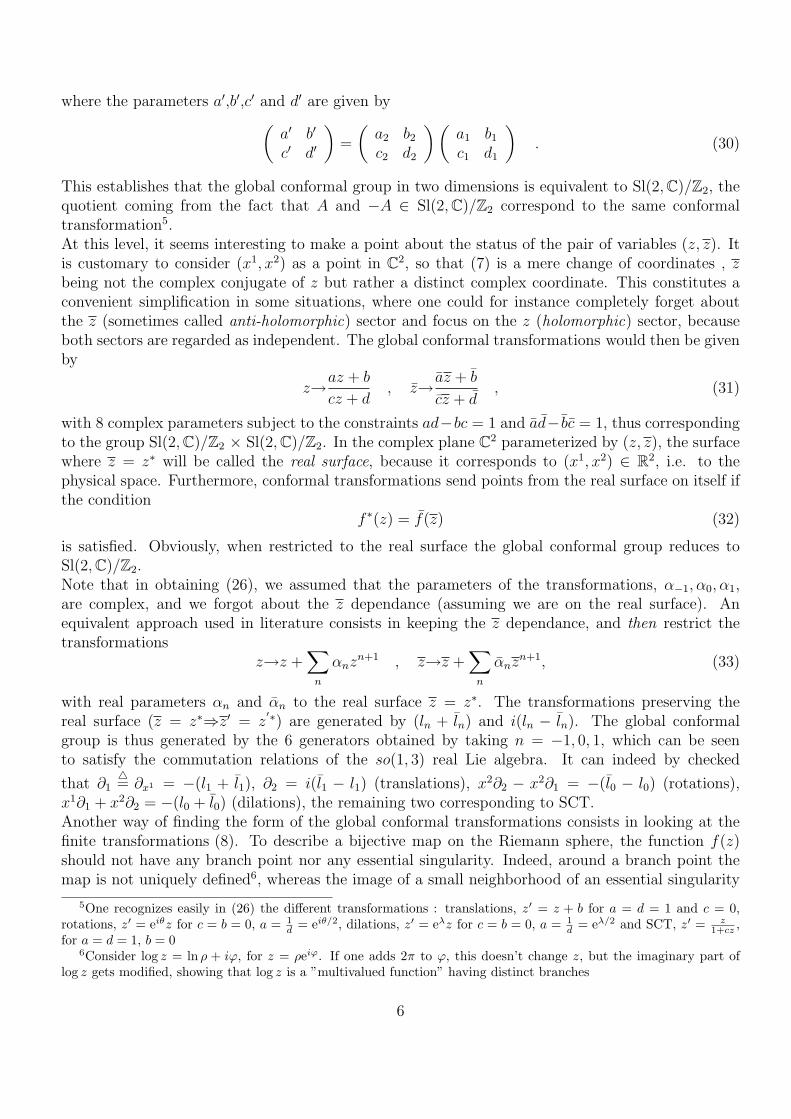
If P (z) has several distinct zeros, then the inverse image of zero is not unique and f is not invertible.If P (z) has a multiple zero z0 of order n > 1, then the image of a small neighborhood of z0 is wrappedn times around zero, and therefore f is not invertible, see Fig.1.

z0

ε

z0 + ε exp iθ

εn

z P(z)=(z-z0)n

nε exp inθ

Figure 1

Thus P (z) must be of the form P (z) = az + b. The same argument holds for Q(z) when looking atthe behavior of f(z) near z = ∞. Thus

f(z) =az + b

cz + d, (35)

with ad−bc 6= 0 in order for the mapping to be invertible (this is the Jacobian of the transformation).Since an overall scaling of all coefficients does not change f , the normalization ad− bc = 1 has beenadopted , so that we recover the Sl(2,C) global conformal group in two dimensions.

2 Conformal Ward identities in two dimensions : part I

2.1 Preliminaries

The objective of a quantum field theory is to determine the scattering amplitudes between variousasymptotic states (free particles). In practice these amplitudes are computed from the correlation

7Any meromorphic function, i.e. holomorphic except at isolated poles, can be expressed as the ratio of twoholomorphic functions. These could be exponential functions or combination thereof, but we exclude them becausethey are periodic in the complex plane and thus not invertible. Furthermore, such functions are even not defined onthe whole Riemann sphere, because (x, y) = (0,∞) and (x, y) = (∞, 0)are supposed to represent the same point (theNorth Pole in the stereographic projection), while ez = ex(cos y + i sin y) is not univocal at this point

7

functions (Green’s functions) via the so-called reduction formulas. The quantum description of aphysical system may be tackled using different methods. One of them, the operator formalism,consists in replacing classical quantities by operators acting on a vector space in which the states ofthe system reside. Another method is called path integration or functional integration, and can berelated to the first one, see e.g. Appendix A of [11]. To begin, we will work in the second formalism(the operator formalism of two dimensional CFT will be discussed in Sect. 4), in which a euclidiancorrelation function of N fields φi(xi) reads

〈φ1(x1) · · ·φN(xN)〉 =1

Z

∫DΦ φ1(x1) · · ·φN(xN) exp(−S[φ]) , (36)

where Z =∫ DΦ exp(−S[φ]), Φ denotes the set of all functionally independent fields in the theory8,

and S[Φ, ∂µΦ] =∫

d2xL(Φ(x), ∂µΦ(x)) is the action.Classically, the invariance of the action under a continuous symmetry9 implies the existence of aconserved current via Noether’s theorem. At the quantum level, a continuous symmetry of the actionand of the functional measure leads to constraints on the correlation functions, which are expressedvia the so-called Ward identities.Before turning to their derivation in the context of 2D CFT, we define the notion of a primary field.Under a conformal map z→w(z), z→w(z), a primary field transforms as

φ(z, z)−→φ′(w(z), w(z)) =

(dw

dz

)−h (dw

dz

)−h

φ(z, z) , (37)

where h (resp. h) is called holomorphic (resp. anti-holomorphic) conformal dimension of the field.Eq. (37) states that a primary field of conformal dimensions (h, h) transforms as the components ofa tensor with h covariant indices z and h covariant indices z. The conformal dimensions are relatedto the spin s and scaling dimension ∆ of the field by s = h− h and ∆ = h + h 10.These fields play a crucial role in conformal field theories, namely because correlation functionsinvolving any field of the theory can be reduced to correlations functions involving only primaryfields. This is one of the properties rendering conformal field theories in two dimensions solvable,where a theory is said to be solved when all correlation function can be written (at least in principle).Fields transforming like (37), but only under global conformal transformations (31) are called quasi-primary.

2.2 A derivation of the conformal Ward identities

I first would like to mention that there are quite a lot seemingly different derivations of the conformalWard identity. In this section, I will present that of [1], which is to my opinion the shortest way toget to the goal and gives a good flavor of how things fit all together. Skeptical readers may wish to

8When one speaks of a field in CFT, it does not necessarily mean that this field figures independently in thefunctional integration measure. For instance, a single boson φ, its derivative ∂µφ and a composite quantity such asthe energy-momentum tensor are called fields, since they are local quantities with a coordinate dependence. However,only some fields are integrated over in the functional integral

9This means that under a transformation x→x′, φ(x)→φ′(x′), we have S′ = S, with S′ =∫D′ ddx′ L(Φ′(x′), ∂′µΦ′(x′)) =

∫D

ddxL(Φ′(x), ∂µΦ′(x)), where D is the integration domain (often D = R2)10The variation of a field under a transformation can be decomposed in δφ(x) = (φ′(x)− φ′(x′)) + (φ′(x′)− φ(x)),

where the second term encodes the spin and scaling properties of the field. For a rotation, z→eiθz, we find φ′(x′) =eiθ(h−h)φ(x), while under a scaling z→eλz, we have φ′(x′) = e−λ(h+h)φ(x)

8

consult another derivation, maybe more precise, based on [2] and presented in Appendix C (see also[2] p123 for an alternative approach to global conformal Ward identities). Later on, I will return tothe these identities in the context of the operator formalism (see Sect. 4.4 and 4.7).To study the consequences of the consequences of the conformal symmetry on correlation functions,it is usually more convenient to consider infinitesimal transformations of the form (8), for small α(z).With w(z) = z +α(z), w(z) = z + α(z), one finds the infinitesimal transformation of a primary field:

δαφ(z, z) = −(hα′(z) + α(z)∂ + hα′(z) + α(z)∂) φ(z, z) . (38)

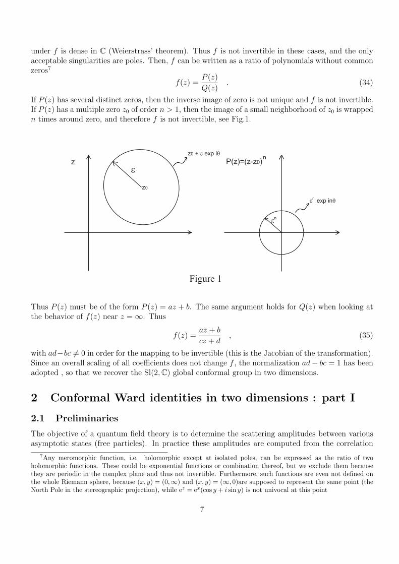
At this point, I would like to draw attention on the infinitesimal character of the transformation weare to use. As we found, general conformal transformations are given by (8), with f(z) and α(z)depending only upon the variable z (I will sometimes omit the z dependence, being understood itis always present). This makes f and α holomorphic functions, except at the location of possiblesingularities. Now, it is clear that close to a singularity, the functions cannot remain infinitesimal,whatever the parameters αn in (12). Furthermore, on the Riemann sphere, even globally holomorphic(analytic) functions (admitting everywhere a Taylor expansion), like polynomials, are unbounded,except the constant function (for another discussion on this point and another way round, see [4],p129).To avoid this problem, we will define transformation (8) in a finite region D, say in the neighborhoodof z = 0, with α(z) analytic in D, and put α(z) = 0 outside D. This way of cutting α(z) will produceboundary terms which we will have to keep track of. The region D will be chosen so to as to containthe positions of all the fields inside the correlation function, see Fig. 2.

.

.

.

x1 x2

xn

D

C

Figure 2

An analytic function in a region D containing the origin may be Taylor expanded around z = 0 as

α(z) =∞∑

n=−1

αnzn+1 . (39)

9

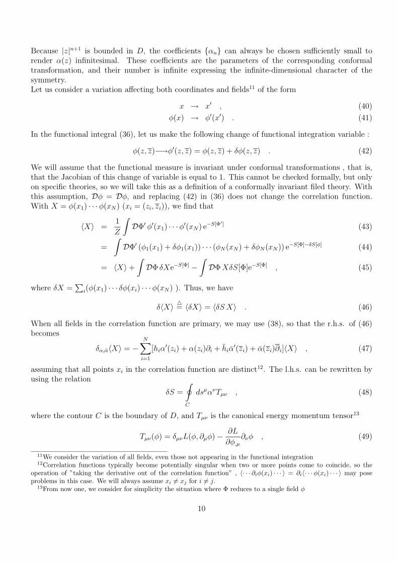
Because |z|n+1 is bounded in D, the coefficients {αn} can always be chosen sufficiently small torender α(z) infinitesimal. These coefficients are the parameters of the corresponding conformaltransformation, and their number is infinite expressing the infinite-dimensional character of thesymmetry.Let us consider a variation affecting both coordinates and fields11 of the form

x → x′ , (40)

φ(x) → φ′(x′) . (41)

In the functional integral (36), let us make the following change of functional integration variable :

φ(z, z)−→φ′(z, z) = φ(z, z) + δφ(z, z) . (42)

We will assume that the functional measure is invariant under conformal transformations , that is,that the Jacobian of this change of variable is equal to 1. This cannot be checked formally, but onlyon specific theories, so we will take this as a definition of a conformally invariant filed theory. Withthis assumption, Dφ = Dφ, and replacing (42) in (36) does not change the correlation function.With X = φ(x1) · · ·φ(xN) (xi = (zi, zi)), we find that

〈X〉 =1

Z

∫DΦ′ φ′(x1) · · ·φ′(xN) e−S[Φ′] (43)

=

∫DΦ′ (φ1(x1) + δφ1(x1)) · · · (φN(xN) + δφN(xN)) e−S[Φ]−δS[φ] (44)

= 〈X〉+

∫DΦ δXe−S[Φ] −

∫DΦ XδS[Φ]e−S[Φ] , (45)

where δX =∑

i(φ(x1) · · · δφ(xi) · · ·φ(xN) ). Thus, we have

δ〈X〉 4= 〈δX〉 = 〈δS X〉 . (46)

When all fields in the correlation function are primary, we may use (38), so that the r.h.s. of (46)becomes

δα,α〈X〉 = −N∑

i=1

[hiα′(zi) + α(zi)∂i + hiα

′(zi) + α(zi)∂i]〈X〉 , (47)

assuming that all points xi in the correlation function are distinct12. The l.h.s. can be rewritten byusing the relation

δS =

∮

C

dsµανTµν , (48)

where the contour C is the boundary of D, and Tµν is the canonical energy momentum tensor13

Tµν(φ) = δµνL(φ, ∂µφ)− ∂L

∂φ,µ

∂νφ , (49)

11We consider the variation of all fields, even those not appearing in the functional integration12Correlation functions typically become potentially singular when two or more points come to coincide, so the

operation of ”taking the derivative out of the correlation function” , 〈· · · ∂iφ(xi) · · · 〉 = ∂i〈· · ·φ(xi) · · · 〉 may poseproblems in this case. We will always assume xi 6= xj for i 6= j.

13From now one, we consider for simplicity the situation where Φ reduces to a single field φ

10

with φ,µ = ∂µφ. This is the conserved current associated with translation invariance of the action.Eq. (48) expresses that, although the action S is supposed to be conformally invariant, we find aboundary term because α(z) is discontinuous on C.Let us derive (48), in the case where αν = aν = cst. Let S[φ] be an action given by

S[φ] =

∫d2xL(φ(x), φ,µ(x)) , (50)

where the lagrangian L is supposed to be local in φ(x) and φ,µ(x), as well as invariant under trans-lations. This implies that

δS[φ] =

∫d2xL(φ′(x), φ′,µ(x)) −

∫d2xL(φ(x), φ,µ(x)) = 0 , (51)

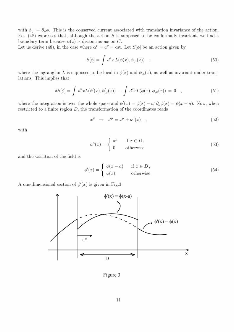
where the integration is over the whole space and φ′(x) = φ(x)− aµ∂µφ(x) = φ(x− a). Now, whenrestricted to a finite region D, the transformation of the coordinates reads

xµ → x′µ = xµ + aµ(x) , (52)

with

aµ(x) =

{aµ if x ∈ D ,

0 otherwise(53)

and the variation of the field is

φ′(x) =

{φ(x− a) if x ∈ D ,

φ(x) otherwise(54)

A one-dimensional section of φ′(x) is given in Fig.3

aµ

Dx

φ'(x) = φ(x-a)

φ'(x) = φ(x)

Figure 3

11

The variation of the action now becomes

δS[φ] =

∫

D

d2xL(φ′(x), φ′,µ(x)) −∫

D

d2xL(φ(x), φ,µ(x)) , (55)

where only the contribution of the part inside D appears. By restricting ourselves to a finite region,we broke translation invariance, in some sense. There are two contributions to δS[φ] in (55). To seethis, we rewrite it as

δS[φ] =

∫

D

d2x

[(∂L

∂φ

)δφ +

(∂L

∂φ,µ

)∂µδφ

](56)

=

∫

D

d2x

[(∂L

∂φ

)− ∂µ

(∂L

∂φ,µ

)]δφ +

∫

D

d2x ∂µ

(∂L

∂φ,µ

δφ

)(57)

4= δSreg[φ] + δSjump[φ] . (58)

The first term corresponds to a ”bulk term”, while the second one can be rewritten using Stokes’theorem as a boundary term, whose contribution comes from the ”jump” that φ experiences on∂D = C :

δSjump[φ]4=

∫

D

d2x ∂µ

(∂L

∂φ,µ

δφ

)=

∮

C

(∂L

∂φ,µ

δφ

)dsµ . (59)

Thus, with δφ = −aν∂νφ ,we get

δSjump[φ] = −∮

C

aν

(∂L

∂φ,µ

)∂νφ dsµ . (60)

The analysis of the regular term is better performed starting directly from (55) and performing thechange of variable x = x − a in the first integral. So, the function to integrate becomes the same,the difference being the integration domains :

δSreg[φ] =

∫

D

d2xL(φ(x), φ,µ(x)) −∫

D

d2xL(φ(x), φ,µ(x)) (61)

=

∫

δD

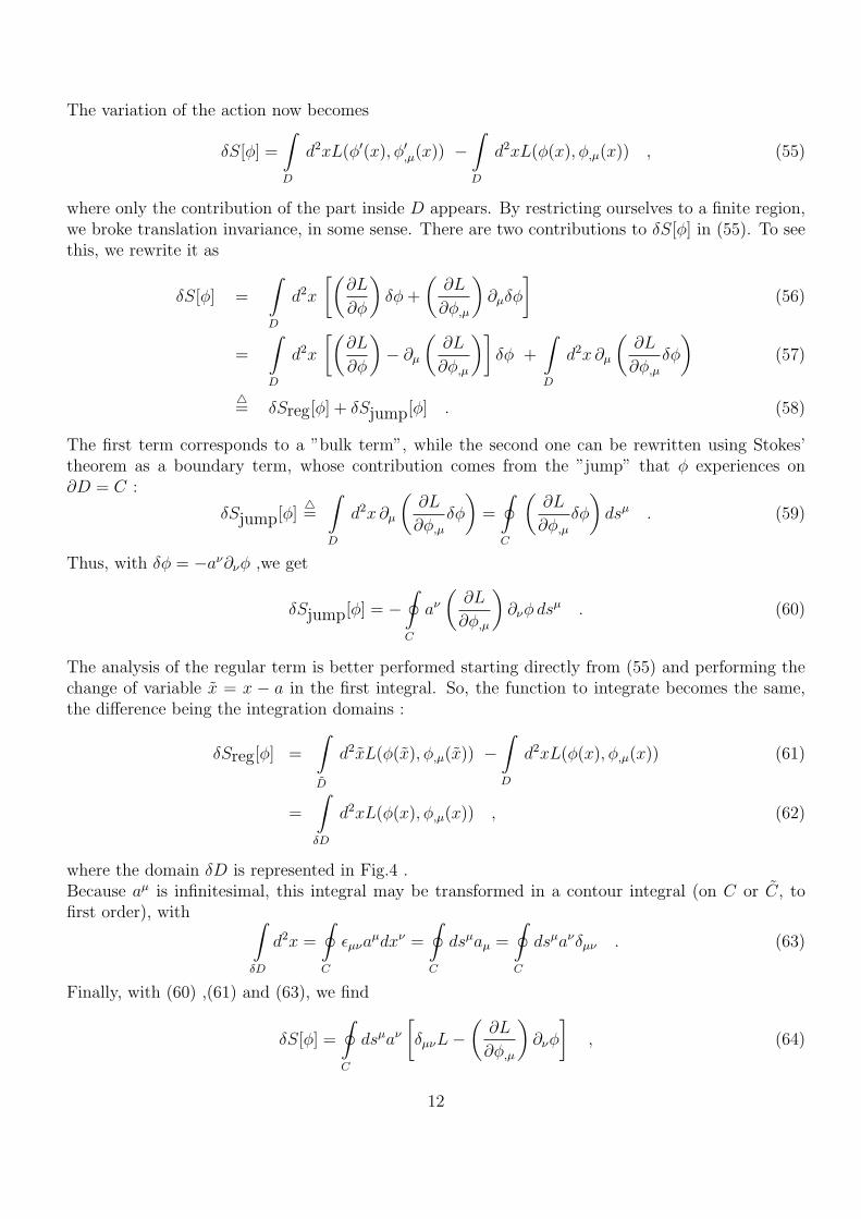
d2xL(φ(x), φ,µ(x)) , (62)

where the domain δD is represented in Fig.4 .Because aµ is infinitesimal, this integral may be transformed in a contour integral (on C or C, tofirst order), with ∫

δD

d2x =

∮

C

εµνaµdxν =

∮

C

dsµaµ =

∮

C

dsµaνδµν . (63)

Finally, with (60) ,(61) and (63), we find

δS[φ] =

∮

C

dsµaν

[δµνL−

(∂L

∂φ,µ

)∂νφ

], (64)

12

δD

δD

Figure 4

dsµ

dxµ x

1

x2

aµ C

C~

and hence Eq. (48). The same argument may still be applied if αµ is replaced by a conformal Killingvector αµ(x). Eq. (46) becomes, using (48)

δ〈X〉 = − 1

2π

∮

c

dsµαν〈TµνX〉 , (65)

where the factor of − 12π

is placed for convenience and corresponds to a normalization choice for Tµν

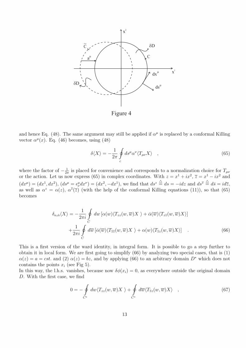
or the action. Let us now express (65) in complex coordinates. With z = x1 + ix2, z = x1 − ix2 and

(dxµ) = (dx1, dx2), (dsµ = εµνdxν) = (dx2,−dx1), we find that dsz 4

= ds = −idz and dsz 4= ds = idz,

as well as αz = α(z), αz(z) (with the help of the conformal Killing equations (11)), so that (65)becomes

δα,α〈X〉 = − 1

2πi

∮

C

dw [α(w)〈Tzz(w, w)X 〉+ α(w)〈Tzz(w, w)X〉]

+1

2πi

∮

C

dw [α(w)〈Tzz(w, w)X 〉+ α(w)〈Tzz(w, w)X〉] . (66)

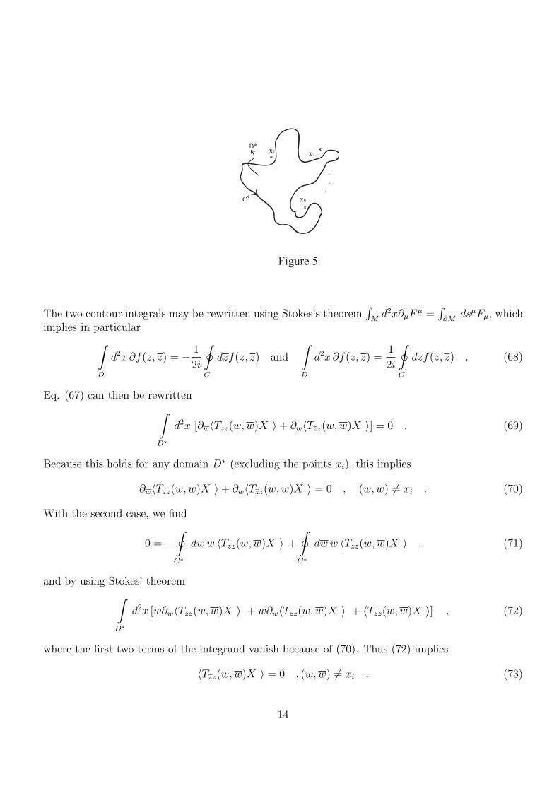
This is a first version of the ward identity, in integral form. It is possible to go a step further toobtain it in local form. We are first going to simplify (66) by analyzing two special cases, that is (1)α(z) = a = cst. and (2) α(z) = bz, and by applying (66) to an arbitrary domain D∗ which does notcontains the points xi (see Fig 5).In this way, the l.h.s. vanishes, because now δφ(xi) = 0, as everywhere outside the original domainD. With the first case, we find

0 = −∮

C∗

dw〈Tzz(w, w)X 〉+

∮

C∗

dw〈Tzz(w, w)X〉 , (67)

13

.

.

.

x1 x2

xn

Figure 5

C*

D*

The two contour integrals may be rewritten using Stokes’s theorem∫

Md2x∂µF

µ =∫

∂MdsµFµ, which

implies in particular

∫

D

d2x ∂f(z, z) = − 1

2i

∮

C

dzf(z, z) and

∫

D

d2x ∂f(z, z) =1

2i

∮

C

dzf(z, z) . (68)

Eq. (67) can then be rewritten

∫

D∗

d2x [∂w〈Tzz(w, w)X 〉+ ∂w〈Tzz(w, w)X 〉] = 0 . (69)

Because this holds for any domain D∗ (excluding the points xi), this implies

∂w〈Tzz(w, w)X 〉+ ∂w〈Tzz(w, w)X 〉 = 0 , (w, w) 6= xi . (70)

With the second case, we find

0 = −∮

C∗

dw w 〈Tzz(w, w)X 〉 +

∮

C∗

dw w 〈Tzz(w, w)X 〉 , (71)

and by using Stokes’ theorem

∫

D∗

d2x [w∂w〈Tzz(w, w)X 〉 + w∂w〈Tzz(w, w)X 〉 + 〈Tzz(w, w)X 〉] , (72)

where the first two terms of the integrand vanish because of (70). Thus (72) implies

〈Tzz(w, w)X 〉 = 0 , (w, w) 6= xi . (73)

14

From (69) and (73), we find that

∂w〈Tzz(w, w)X 〉 = 0 , (w, w) 6= xi . (74)

Similar relations hold for 〈Tzz(w, w)X 〉 and ∂w〈Tzz(w, w)X 〉, so that we end up with

∂w〈Tzz(w, w)X 〉 = ∂w〈Tzz(w, w)X 〉 = 0 if (w, w) 6= (wi, wi) (75)

and〈Tzz(w, w)X 〉 = 〈Tzz(w, w)X 〉 = 0 if (w, w) 6= (wi, wi) . (76)

Eq. (75) shows that inside correlation functions Tzz (resp. Tzz) does not depend on z (resp. z), andis said to be an holomorphic operator (resp. anti-holomorphic operator), except at the points xi. Weset

Tzz4= T (z) and Tzz

4= T (z) . (77)

Furthermore, T µµ = gµνTµν = T11 + T22 = 1

2(Tzz + Tzz), so (76) expresses the vanishing of the trace

of the energy-momentum tensor inside a correlation function except at coincident points1415 Finally,eq. (66) reduces, with (75), (76) and (77), to16

δα,α〈X〉 = − 1

2πi

∮

C

dwα(w)〈T (w)X 〉+1

2πi

∮

C

dwα(w)〈T (w)X 〉 . (78)

Because of the form of (47) and (78), we observe that (78) splits into two independent equations(recall we may consider z and z as two independent variables, as well as α(z) and α(z) as twoindependent functions). Let us focus on the z-part (”holomorphic” part), and consider a correlationfunction involving primary fields :

− 1

2πi

∮

C

dwα(w)〈T (w)X 〉 = −∑

i

(α′(zi)hi + α(zi)∂i)〈X〉 . (79)

Using the residue theorem17, the r.h.s. may be rewritten as

− 1

2πi

N∑i=1

∮

Ci

dwα(w)

(hi

(w − zi)2+

1

w − zi

∂i

)〈X〉 , (80)

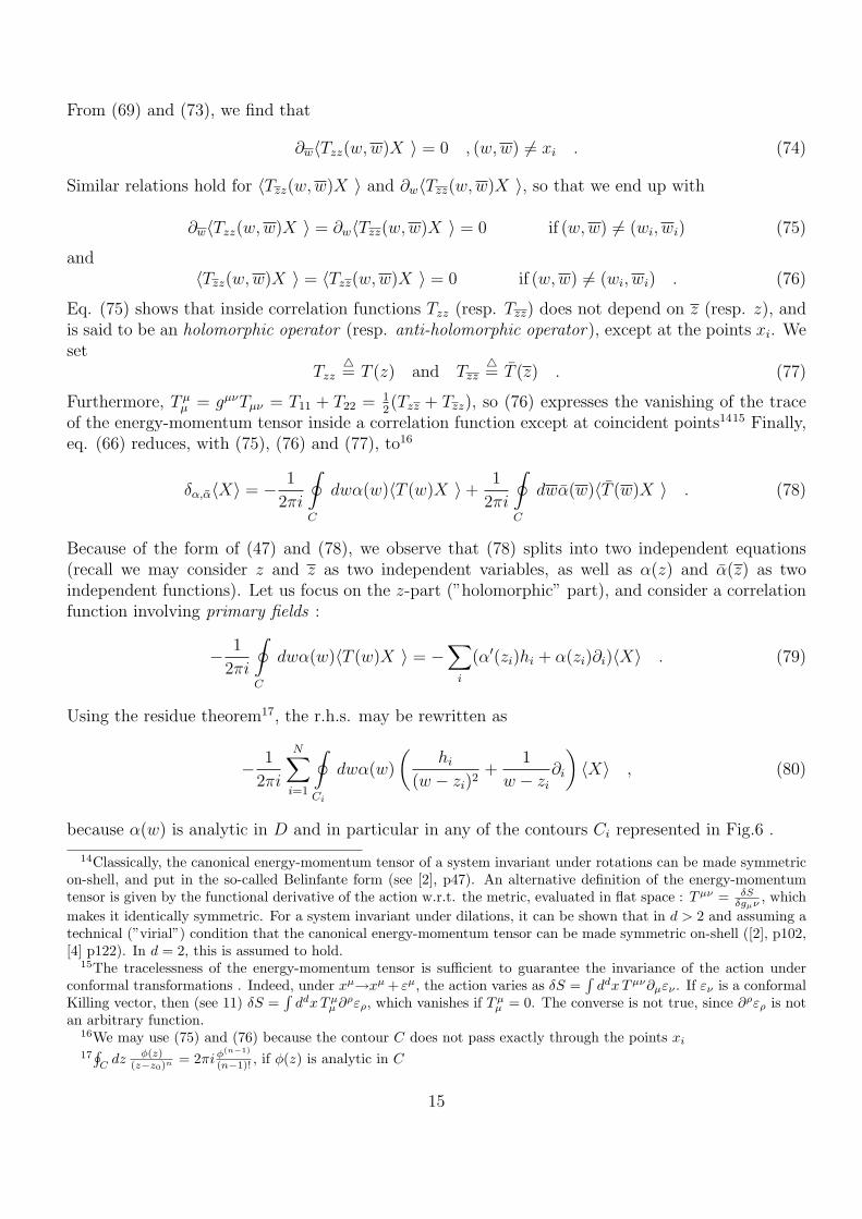
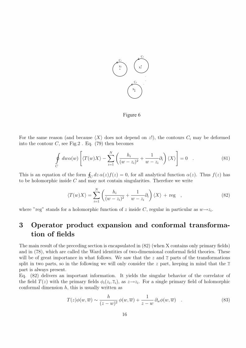
because α(w) is analytic in D and in particular in any of the contours Ci represented in Fig.6 .

14Classically, the canonical energy-momentum tensor of a system invariant under rotations can be made symmetricon-shell, and put in the so-called Belinfante form (see [2], p47). An alternative definition of the energy-momentumtensor is given by the functional derivative of the action w.r.t. the metric, evaluated in flat space : Tµν = δS

δgµν , whichmakes it identically symmetric. For a system invariant under dilations, it can be shown that in d > 2 and assuming atechnical (”virial”) condition that the canonical energy-momentum tensor can be made symmetric on-shell ([2], p102,[4] p122). In d = 2, this is assumed to hold.

15The tracelessness of the energy-momentum tensor is sufficient to guarantee the invariance of the action underconformal transformations . Indeed, under xµ→xµ + εµ, the action varies as δS =

∫ddxTµν∂µεν . If εν is a conformal

Killing vector, then (see 11) δS =∫

ddx Tµµ ∂ρερ, which vanishes if Tµ

µ = 0. The converse is not true, since ∂ρερ is notan arbitrary function.

16We may use (75) and (76) because the contour C does not pass exactly through the points xi

17∮

Cdz φ(z)

(z−z0)n = 2πiφ(n−1)

(n−1)! , if φ(z) is analytic in C

15

.

.

.

x1 x2

xn

Figure 6

Cn

C1

C2

For the same reason (and because 〈X〉 does not depend on z!), the contours Ci may be deformedinto the contour C, see Fig.2 . Eq. (79) then becomes

∮

C

dwα(w)

[〈T (w)X〉 −

N∑i=1

(hi

(w − zi)2+

1

w − zi

∂i

)〈X〉

]= 0 . (81)

This is an equation of the form∮

Cdz α(z)f(z) = 0, for all analytical function α(z). Thus f(z) has

to be holomorphic inside C and may not contain singularities. Therefore we write

〈T (w)X〉 =N∑

i=1

(hi

(w − zi)2+

1

w − zi

∂i

)〈X〉 + reg , (82)

where ”reg” stands for a holomorphic function of z inside C, regular in particular as w→zi.

3 Operator product expansion and conformal transforma-

tion of fields

The main result of the preceding section is encapsulated in (82) (when X contains only primary fields)and in (78), which are called the Ward identities of two-dimensional conformal field theories. Thesewill be of great importance in what follows. We saw that the z and z parts of the transformationssplit in two parts, so in the following we will only consider the z part, keeping in mind that the zpart is always present.Eq. (82) delivers an important information. It yields the singular behavior of the correlator ofthe field T (z) with the primary fields φi(zi, zi), as z→zi. For a single primary field of holomorphicconformal dimension h, this is usually written as

T (z)φ(w, w) ∼ h

(z − w)2φ(w, w) +

1

z − w∂wφ(w, w) . (83)

16

The precise meaning of this expression is the following : when z→w, the (correlation) function〈T (z)φ(w, w)Y 〉 behaves as the function h

(z−w)2〈φ(w, w)Y 〉+ 1

z−w∂w〈φ(w, w)Y 〉, where

Y = φ1(w1, w1) · · ·φn(wn, wn), none of the points being coincident in 〈T (z)φ(w, w)Y 〉. An expressionlike (83) is called (the singular part of) the operator product expansion (or OPE ) of the energy-momentum tensor with a primary field. As we stressed, it only makes sense inside a correlationfunction. The symbol ” ∼ ” means equality up to terms which are regular as z→w. A general OPEof two fields takes the form

A(z)B(w) =N∑

n=−∞

{AB}n(w)

(z − w)n∼

N∑n=1

{AB}n(w)

(z − w)n, (84)

where the composite fields {AB}n(w) are non-singular at w = z. For instance, {Tφ}1(w) = ∂wφ(w).Let us now return to eq. (78), focusing on the z part :

δα〈X〉 = − 1

2πi

∮

C

dw α(w)〈T (w)X〉 , (85)

where δα〈X〉 stands for 〈(δαφ1)φ2 · · ·φN〉+ · · ·+ 〈φ1 · · · (δαφN)〉 as before. This Ward identity can beinterpreted as defining the transformation of the fields within the correlation function. The variationof the function on the l.h.s. is by definition that produced by the variation of the operators. Nowremember the contour C encircles the positions of all operators. This contour may be ”distributed”on the operators φ1, · · · , φN as in Fig.6, because the only singular points of 〈T (w)X〉 are located atw = zi. Thus

δα〈φ1 · · ·φN〉 4=

N∑

k=1

〈φ1 · · · δα(zk)φk(zk) · · ·φN〉 (86)

=N∑

k=1

1

2πi

∮

Ck

dw α(w)〈T (w)φ1 · · ·φN〉 . (87)

Each integral in (87) corresponds to the variation of a field in (86). So, the variation of a single fieldis represented by the integral

δα(zi)φ(zi) =1

2πi

∮

Ci

dw α(w)T (w)φi(zi) , (88)

where Ci encircles only zi, see Fig.6. Consequently, because α(z) is analytic inside Ci, we concludethat the transformation of a field under z→z+α(z) is completely determined by the singular terms ofthe OPE of this field with the holomorphic part T (z) of the energy-momentum tensor, and vice-versa.This explains the important role of OPE’s in conformal field theories.We now concentrate on the transformation properties of the holomorphic energy-momentum tensor,T (z). From its definition, it seems natural that it should transform as a rank 2 covariant tensor,

T (z)−→T ′(w) =

(dw

dz

)−2

T (z) (89)

under z→w(z), thus as a primary field of conformal weight h = 2, h = 0 (see eq.(37)) (similarly,T (z) should have h = 0, h = 2. Actually, it turns out, in passing to the quantum theory, that the

17

situation is complicated by the addition of a term in the transformation law (89), so that the latterbecomes in general

T (z)−→T ′(w) =

(dw

dz

)−2 [T (z)− c

12{w; z}

], (90)

where cis a numerical constant characterizing the theory and where

{w; z} 4=

d3w/dz3

dw/dz− 3

2

(d2w/dz2

dw/dz

)2

(91)

is called the Schwartzian derivative. The additional term in (90) is called Schwinger term and isrelated, as we will see in Sect. 4.2, to the conformal anomaly. It can be shown (see for instance[4], pp134-141) that, requiring that (90) defines a group law and that (91) be a local functional (i.e.containing derivatives of w(z) only up to finite order and degree), the form of the functional (91) iscompletely fixed up to a constant, hence the term c

1218. Notice that the Schwartzian derivative of

the global conformal map

w(z) =az + b

cz + d, ad− bc = 1 (92)

vanishes, making T (z) a quasi-primary field of conformal weight h = 2. The infinitesimal variationδαT (z) = T ′(z)− T (z) can be obtained from (91) by considering {z + α(z), z} to first order in α :

{z + α(z), z} =∂3α

1 + ∂α− 3

2

(∂2α

1 + ∂α

)2

∼ ∂3α (93)

then (90) gives

T ′(z + α) = (1− 2∂α(z))[T (z)− c

12∂3α

]

= T ′(z) + α(z)∂T (z) , (94)

henceδαT (z) = T ′(z)− T (z) = − c

12∂3α− 2∂α(z)T (z)− α(z)∂T (z) . (95)

An alternative way of proceeding is to consider the OPE of T (z) with itself which, according tothe discussion of preceding section and eq. (88), should encode (95). It again turns out that, for ageneral CFT, this OPE has the form

T (z)T (w) ∼ c/2

(z − w)4+

2T (w)

(z − w)2+

∂T (w)

z − w. (96)

Given a specific CFT, (96) is generally easier to obtain by standard techniques than (95), as we willsee on some particular examples in the exercises (see also [2] pp128-135, p138). The last two terms of(96) again reflect the fact that T (z) is a quasi-primary field of conformal dimension h = 2 (see (83)).

The term c/2(z−w)4

is actually the only addition compatible with the scaling transformation of (96). Let

18The group property to be verified is that the result of two successive transformations z→w→u should coin-cide with what is obtained from the single transformation z→u, that is T ′′(u) =

(dudw

)−2 [T ′(w)− c

12{u;w}] =(dudw

)−2[(

dwdz

)−2(T (z)− c

12{w; z})− c12{u; w}

]!=

(dudz

)−2 [T (z)− c

12{u; z}]. The last equality requires the following

relation between the Schwartzian derivatives : {u; z} = {w; z}+(

dwdz

)−2 {u; w}, which is indeed satisfied.

18

us see that (95) and (96) really expresses the same thing. The relation between the variation of afield and the OPE is given by (88). By plugging (96) in (88), we get

δαT (z) = − 1

2πi

∮

Cz

dw α(w)T (w)T (z)

= − 1

2πi

∮

Cz

dw α(w)

[c/2

(w − z)4+

2T (z)

(w − z)2+

∂T (z)

w − z

], (97)

so that after performing the integration, we effectively recover (95).

4 Operator formalism

Throughout the previous sections, all our manipulations were assumed to hold inside correlationfunctions. The consequences of conformal symmetry on two-dimensional field theories were embodiedin constraints imposed on these correlation functions via the Ward identities (78) (we will elaborateon this point in Sect 4.4). These Ward identities were most easily expressed in the form of an OPEof the energy-momentum tensor with local fields (see (83) and (96)). Up to now, we only used thepath-integral representation of the theory in which all correlation functions could in principle beobtained. We would now like to give an operator interpretation in terms of states in a Hilbert space.

4.1 Radial quantization

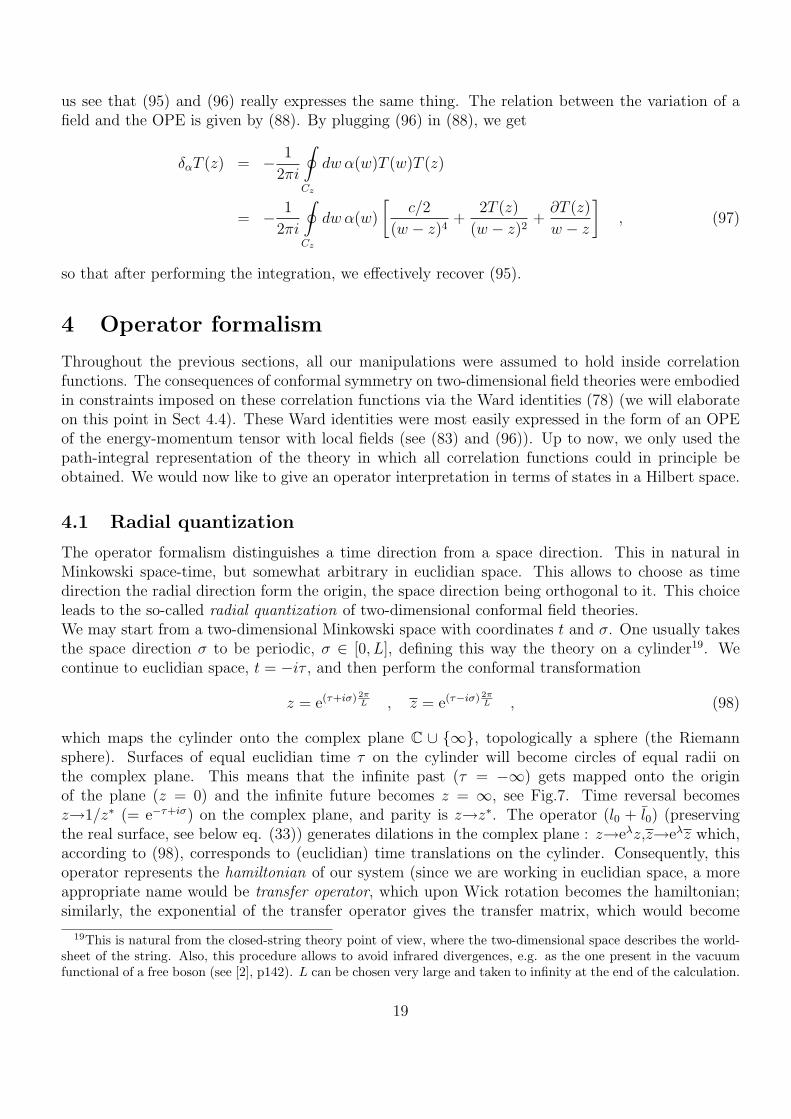
The operator formalism distinguishes a time direction from a space direction. This in natural inMinkowski space-time, but somewhat arbitrary in euclidian space. This allows to choose as timedirection the radial direction form the origin, the space direction being orthogonal to it. This choiceleads to the so-called radial quantization of two-dimensional conformal field theories.We may start from a two-dimensional Minkowski space with coordinates t and σ. One usually takesthe space direction σ to be periodic, σ ∈ [0, L], defining this way the theory on a cylinder19. Wecontinue to euclidian space, t = −iτ , and then perform the conformal transformation

z = e(τ+iσ) 2πL , z = e(τ−iσ) 2π

L , (98)

which maps the cylinder onto the complex plane C ∪ {∞}, topologically a sphere (the Riemannsphere). Surfaces of equal euclidian time τ on the cylinder will become circles of equal radii onthe complex plane. This means that the infinite past (τ = −∞) gets mapped onto the originof the plane (z = 0) and the infinite future becomes z = ∞, see Fig.7. Time reversal becomesz→1/z∗ (= e−τ+iσ) on the complex plane, and parity is z→z∗. The operator (l0 + l0) (preservingthe real surface, see below eq. (33)) generates dilations in the complex plane : z→eλz,z→eλz which,according to (98), corresponds to (euclidian) time translations on the cylinder. Consequently, thisoperator represents the hamiltonian of our system (since we are working in euclidian space, a moreappropriate name would be transfer operator, which upon Wick rotation becomes the hamiltonian;similarly, the exponential of the transfer operator gives the transfer matrix, which would become

19This is natural from the closed-string theory point of view, where the two-dimensional space describes the world-sheet of the string. Also, this procedure allows to avoid infrared divergences, e.g. as the one present in the vacuumfunctional of a free boson (see [2], p142). L can be chosen very large and taken to infinity at the end of the calculation.

19

τ

σ

|z| = cst.

τ=− 8

z

z = exp (τ+iσ)2π/L

Figure 7

the time evolution operator upon Wick rotation). Finally, an integral over the space direction σ, atfixed τ , will become a contour integral on the complex plane. This enables us to use all the powerfultechniques of complex analysis. We would now like to translate a relation like (85) :

δα(z)〈X〉 = − 1

2πi

∮

C

dw α(w)〈T (w)X〉

in the operator formalism language. Expressions like 〈φ(z1, z1)φ(z2, z2)〉 which were understood inthe path integral formalism (see (36)) must now be interpreted as

〈 0 |T (φ(τ1, σ1)φ(τ2, σ2)| 0 〉 , (99)

where | 0 〉 is the vacuum state of the Hilbert space of states H (see Sect. 4.3) and where thefields become operators acting on H. As is known (see Appendix B for a reminder), in ordinaryQFT insertion of operators in the path integral represents time-ordered matrix elements of thecorresponding operators. The time-ordering, defined by

T [φ(τ1, σ1)φ(τ2, σ2)] =

{φ(τ1, σ1)φ(τ2, σ2) if τ1 > τ2 ,

εφ(τ2, σ2)φ(τ1, σ1) if τ2 > τ1

(100)

where ε = 1 for bosons and −1 for fermions, appears naturally by the nature of the path integral,which builds amplitudes from successive time steps. In radial quantization, this notion obviouslygeneralizes to the radial-ordering

R [φ(z1, z1)φ(z2, z2)] =

{φ(z1, z1)φ(z2, z2) if |z1| > |z2| ,εφ(z2, z2)φ(z1, z1) if |z2| > |z1|

(101)

Since all fields within correlation functions must be radially ordered, so must be the l.h.s. of any OPEif it is to have an operator meaning. In particular, all OPE’s written previously have an operatormeaning if |z| > |w|.

20

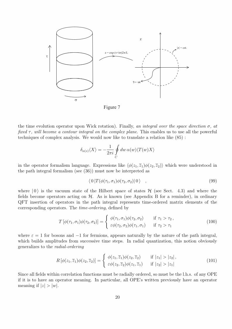
Recall that in (88), C is a contour encircling all points zi appearing in X = φ1 · · ·φN . Let us considerthe variation of a single operator, X = φ(z, z) :

δα(z)φ(z, z) = − 1

2πi

∮

C

dw α(w)R [T (w)φ(z, z)] (102)

where C is represented in Fig.8 . We will forget about the z dependence in what follows. As we

C

z

w

Figure 8

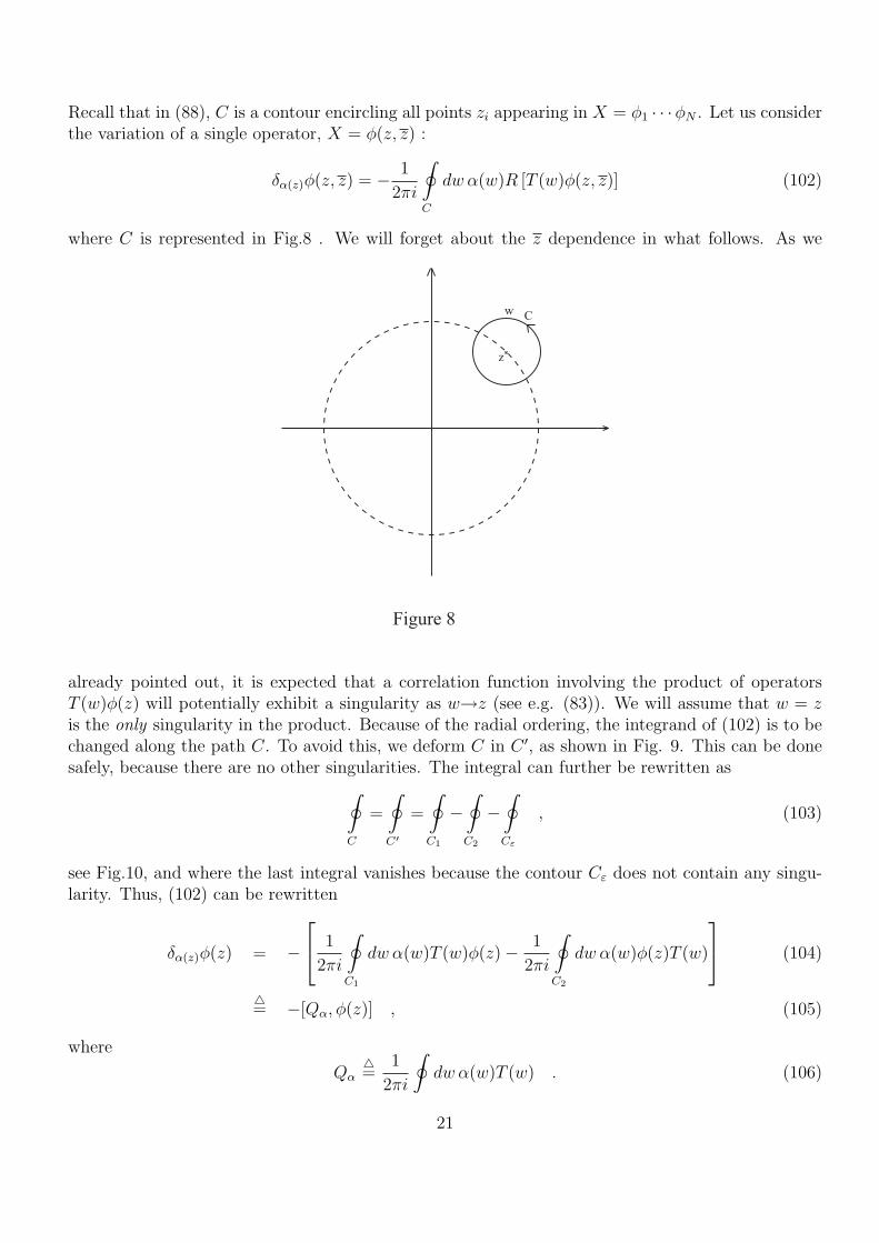
already pointed out, it is expected that a correlation function involving the product of operatorsT (w)φ(z) will potentially exhibit a singularity as w→z (see e.g. (83)). We will assume that w = zis the only singularity in the product. Because of the radial ordering, the integrand of (102) is to bechanged along the path C. To avoid this, we deform C in C ′, as shown in Fig. 9. This can be donesafely, because there are no other singularities. The integral can further be rewritten as

∮

C

=

∮

C′

=

∮

C1

−∮

C2

−∮

Cε

, (103)

see Fig.10, and where the last integral vanishes because the contour Cε does not contain any singu-larity. Thus, (102) can be rewritten

δα(z)φ(z) = − 1

2πi

∮

C1

dw α(w)T (w)φ(z)− 1

2πi

∮

C2

dw α(w)φ(z)T (w)

(104)

4= −[Qα, φ(z)] , (105)

where

Qα4=

1

2πi

∮dw α(w)T (w) . (106)

21

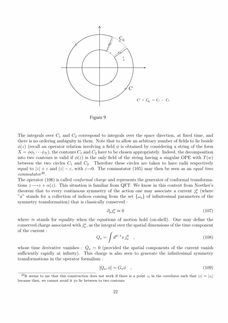
Figure 9

C ε

C'

z

C' + C = C1 - C2 ε

The integrals over C1 and C2 correspond to integrals over the space direction, at fixed time, andthere is no ordering ambiguity in them. Note that to allow an arbitrary number of fields to lie besideφ(z) (recall an operator relation involving a field φ is obtained by considering a string of the formX = φφ1 · · ·φN), the contours C1 and C2 have to be chosen appropriately. Indeed, the decompositioninto two contours is valid if φ(z) is the only field of the string having a singular OPE with T (w)between the two circles C1 and C2. Therefore these circles are taken to have radii respectivelyequal to |z| + ε and |z| − ε, with ε→0. The commutator (105) may then be seen as an equal timecommutator 20.The operator (106) is called conformal charge and represents the generator of conformal transforma-tions z−→z + α(z). This situation is familiar from QFT. We know in this context from Noether’stheorem that to every continuous symmetry of the action one may associate a current jµ

a (where”a” stands for a collection of indices coming from the set {ωa} of infinitesimal parameters of thesymmetry transformation) that is classically conserved :

∂µjµa ≈ 0 (107)

where ≈ stands for equality when the equations of motion hold (on-shell). One may define theconserved charge associated with jµ

a , as the integral over the spatial dimensions of the time componentof the current :

Qa =

∫dd−1x j0

a , (108)

whose time derivative vanishes : Qa = 0 (provided the spatial components of the current vanishsufficiently rapidly at infinity). This charge is also seen to generate the infinitesimal symmetrytransformations in the operator formalism :

[Qa, φ] = Gaφ , (109)

20It seems to me that this construction does not work if there is a point zi in the correlator such that |z| = |zi|because then, we cannot avoid it yo lie between to two contours

22

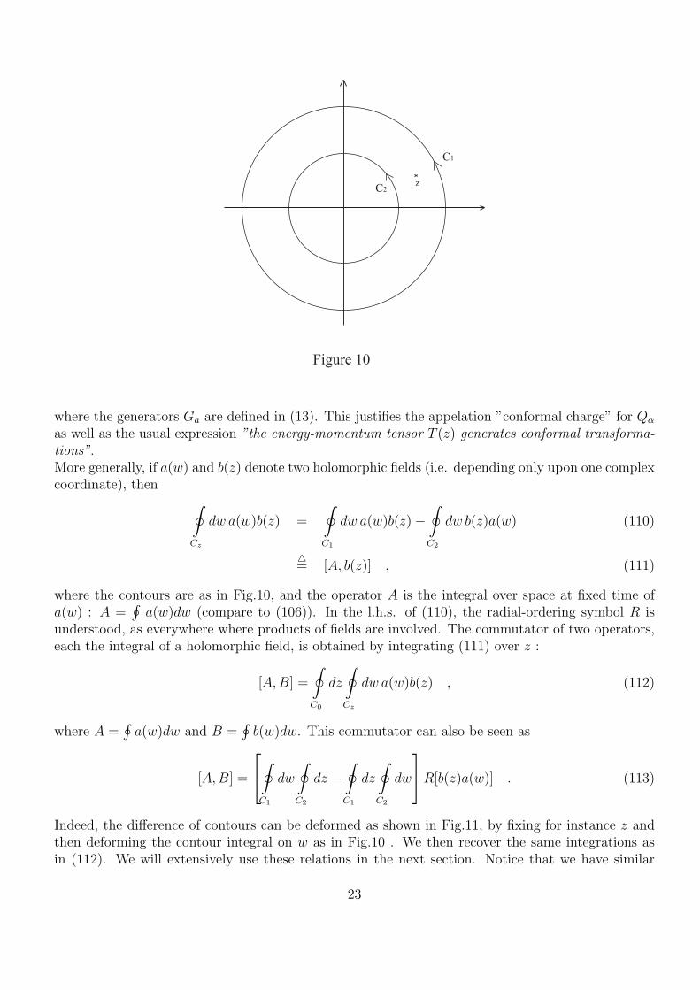
Figure 10

z

C1

C2

where the generators Ga are defined in (13). This justifies the appelation ”conformal charge” for Qα

as well as the usual expression ”the energy-momentum tensor T (z) generates conformal transforma-tions”.More generally, if a(w) and b(z) denote two holomorphic fields (i.e. depending only upon one complexcoordinate), then

∮

Cz

dw a(w)b(z) =

∮

C1

dw a(w)b(z)−∮

C2

dw b(z)a(w) (110)

4= [A, b(z)] , (111)

where the contours are as in Fig.10, and the operator A is the integral over space at fixed time ofa(w) : A =

∮a(w)dw (compare to (106)). In the l.h.s. of (110), the radial-ordering symbol R is

understood, as everywhere where products of fields are involved. The commutator of two operators,each the integral of a holomorphic field, is obtained by integrating (111) over z :

[A,B] =

∮

C0

dz

∮

Cz

dw a(w)b(z) , (112)

where A =∮

a(w)dw and B =∮

b(w)dw. This commutator can also be seen as

[A,B] =

∮

C1

dw

∮

C2

dz −∮

C1

dz

∮

C2

dw

R[b(z)a(w)] . (113)

Indeed, the difference of contours can be deformed as shown in Fig.11, by fixing for instance z andthen deforming the contour integral on w as in Fig.10 . We then recover the same integrations asin (112). We will extensively use these relations in the next section. Notice that we have similar

23

- =

w

C1

z

C2

z

C1

w

C2

O

z

w

becausez

w

= C1 - C2

C1

C2

Figure 11

relations for operators defined by a contour integration around an arbitrary point : A(z) =∮

za(w)dw.

This integral does not represent a fixed-time integral, but the commutation of two such operatorscan still be defined through (112) and (113) by replacing the point z = 0 by an arbitrary z.From now on, whenever a contour integral is written without a specific contour, it is understood thatwe integrate at fixed time, i.e. along a circle centered at the origin. Otherwise the relevant pointssurrounded by the contours are indicated below the integral sign.As a conclusion, formulas (111) and (112) are important because they allow to relate OPE’s tocommutation relations, as we will see in the next section.

4.2 Mode expansions and Virasoro algebra

A conformal field (primary or quasi-primary) of dimensions (h, h) may be mode expanded as follows:

φ(z, z) =∑

m,n∈Zz−m−hz−n−h φm,n , (114)

with

φm,n =1

2πi

∮dz zm+h−1φ(z, z)

1

2πi

∮dz zm+h−1φ(z, z) . (115)

With this definition, the modes transform under scaling z→λz as φn→φ′n = λnφn, thus having scalingdimension n. Eq. (114) corresponds to a Laurent expansion around z = 0. Later on we will use adevelopment around a arbitrary point w :

φ(z, z) =∑

m,n∈Z(z − w)−m−h(z − w)−n−h φm,n(w, w) , (116)

with

φm,n(w, w) =1

2πi

∮dz (z − w)m+h−1φ(z, z)

1

2πi

∮dz (z − w)m+h−1φ(z, z) . (117)

24

We set hereafter φm,n(0, 0)4= φm,n.

For the energy-momentum tensor, we have

T (z) =∑

n∈Zz−n−2Ln , T (z) =

∑

n∈Zz−n−2Ln , (118)

where the modes are given by the contour integrals

Ln =1

2πi

∮dz zn+1T (z), Ln =

1

2πi

∮dz zm+1T (z) . (119)

Considering an infinitesimal conformal transformation z→z + α(z), with α(z) =∑

n zn+1αn, theconformal charge (106) can be reexpressed as

Qα =1

2πi

∑n

∮dw αnwn+1T (w) =

∑n

αnLn . (120)

The variation of a field then reads with (105)

δα(z)φ(z) = −∑

n

αn[Ln, φ(z)] . (121)

In particular , for a transformation z→z + αnzn+1 4

= z + αn(z), we have

δαn(z)φ(z) = −αn[Ln, φ(z)] . (122)

The mode operators Ln (and similarly Ln, which we will omit) are the generators of the localconformal transformations on the Hilbert space, exactly like ln (and ln) (see (15)) are the generatorsof conformal mappings on the space of functions21. Using (111), the algebra they satisfy may bederived, with the help of the OPE (96) :

[Ln, Lm] =1

(2πi)2

∮

0

dw

∮

w

dz zn+1wm+1 T (z)T (w)

=1

(2πi)2

∮

0

dw

∮

w

dz zn+1wm+1

[c/2

(z − w)4+

2T (w)

(z − w)2+

∂T (w)

z − w

]

=1

2πi

∮

0

dw wm+1

[c/2

3!∂3(zn+1) + 2T (w)∂(zn+1) + ∂T (w)zn+1

]

|z=w

=1

2πi

∮

0

dw[ c

12wm+n−1n(n2 − 1) + 2T (w)(n + 1)wm+n+1 + wm+n+2

]

= n(n2 − 1)c

12δm+n,0 + 2(n + 1)Lm+n

+1

2πi

∮

0

dw∂(wm+n+2T (w))−∮

0

dwT (w)(m + n + 2)wm+n+1

, (123)

21Recall the Ln’s generate the conformal transformations of the operators φ

25

hence[Ln, Lm] =

c

12n(n2 − 1)δm+n,0 + (n−m)Lm+n . (124)

A similar relation holds for the Ln’s and [Ln, Lm] = 0. This is the Virasoro algebra. It can be seenas a central extension of the Witt algebra (16). It is clear that the central term proportional to c isdue to the presence of the Schwinger term in (90) and (96). We note that the generators L−1,L0 andL1 form a Sl(2,C) subalgebra identical to that generated by the ln’s for n = −1, 0, 1 :

[L−1, L0] = −L−1 , [L1, L0] = L1 , [L1, L−1] = 2L0 . (125)

Thus, only the global subgroup Sl(2,C) is not affected by the conformal anomaly. This will bereflected when returning to the Ward identities in Sect. 4.4, where we will see that the correlationfunctions are invariant only under the global conformal group.

4.3 The Hilbert space and representations of the Virasoro algebra

To describe the Hilbert space H, we will use the standard formalism of ”in” and ”out” states ofquantum field theory. We first have to assume the existence of a vacuum state | 0 〉 upon which His constructed by application of creation operators (or their likes). In free field theories (in the QFTsense), the vacuum may be defined as the state annihilated by the positive frequency part of the field.For an interacting field, we assume following the usual procedure of QFT that the Hilbert space isthe same as for a free field, except that the actual energy eigenstates are different. We suppose thatthe ic interaction is attenuated as t→±∞ and that asymptotic fields are free.In a two-dimensional CFT on the complex plane, the in-states are defined as

|φin 〉 = limz,z→0

φ(z, z)| 0 〉 , (126)

for some quasi-primary field φ(z, z). On H, we must also define a bilinear product, which we doindirectly by defining asymptotic out-states together with the action of Hermitian conjugation onconformal fields. One sets

〈φout | = |φin 〉+ , (127)

with

[φ(z, z)]+4= z−2hz−2h φ(

1

z,1

z) , (128)

where φ is a quasi-primary field of dimensions (h, h). In Minkowski space, Hermitian conjugation doesnot affect the space-time coordinates, while in euclidian space, τ = it must be reversed (τ→−τ) uponHermitian conjugation if t is to be left unchanged. So this corresponds to the mapping z→ 1

z∗ = 1z

on the real surface (see Sect. 4.1 and (98)) and explains the interchange z→1z, z→1

zin (128). The

additional factors on the r.h.s. of (128) may be justified by demanding that the inner product〈φout |φin〉 is well-defined22. Let us focus on the holomorphic part of the stress-energy tensor. Bytaking the adjoint of the mode expansion (118), one finds on the one hand

[T (z)]+ =∑

n

z−n−2L+n , (129)

22〈φout |φin〉 = limz,z,w,w→0

〈 0 |φ(z, z)φ(w, w)| 0 〉 = lim z−2hz−2h〈 0 |φ(1/z, 1/z)φ(w, w)| 0 〉 =

limξ,ξ→0

〈 0 |φ(ξ, ξ)φ(w, w)| 0 〉ξ2hξ2h. We will see in Sect 4.4 that the 2-point functions are completely fixed by

conformal invariance, and have the form 〈φ(ξ, ξ)φ(w, w)〉 = Cξ2hξ2h , so that the product is well defined because the

factors cancel out. See also [5] p52, [4] p147.

26

and on the other hand, from (128)

[T (z)]+ = z−4T (1/z) = z−4∑

n

zn+2Ln =∑m

z−m−2L−m . (130)

These expressions are compatible if

L+n = L−n , and similarly L+

n = L−n . (131)

We may also determine the action of the Ln’s on H. With (117) and (119), we have

Ln(z)φ(z, z)4= (Lnφ)(z, z) =

1

2πi

∮

z

dw (w − z)n+1 T (w)φ(z, z) . (132)

Consider a primary field φ(z) of conformal weight h (leaving the anti-holomorphic part aside) andthe asymptotic state

|h 〉 4= φ(0)| 0 〉 . (133)

Acting with the Ln’s on this state yields

(Lnφ)(0)4= Ln|h 〉 =

1

2πi

∮

0

dw wn+1T (w)φ(0)| 0 〉 . (134)

Using the OPE (83), one gets

Ln|h 〉 =1

2πi

∮

0

dw wn+1

[h

w2φ(0) +

1

w∂φ(0) + reg

]| 0 〉 (135)

=1

2πi

∮

0

dw[hwn−1φ(0) + wn∂φ(0) + wn+1.reg

] | 0 〉 . (136)

For n ≥ −1, none of the regular terms of the OPE will contribute the integral. We thus find that

Ln|h 〉 = 0 if n > 0 , L0|h 〉 = h|h 〉 (137)

Remark we also have following the same computation that (Lnφ)(w) = 0 for n > 0 and (L0φ)(w) =hφ(w).Eq. (137) defines a highest weight representation of the Virasoro algebra (124)23 of , just like the onesone usually encounters in the su(2) case (see the Lectures on Lie algebras).The operator L0 measuresthe conformal dimension of the state, while the Ln’s play the role of the raising and lowering operators,taking one state to another into a representation. The major difference between the Virasoro (estarriveeee) representations and those of su(2) is of course that the Virasoro representations are infinite-dimensional. Although the algebra is infinite-dimensional, the Cartan subalgebra (i.e. the maximalset of commuting Hermitian generators) contains just the identity operator and L0 (from (124), we

23Representations of the anti-holomorphic counterpart of (124) are constructed by the same method. Since the twoparts of the overall algebra decouples ([Ln, Lm] = 0), representations of the latter are obtained simply by taking tensorproducts

27

see that no pair of generators commute, so we may choose L0 which, from (137), is diagonal in therepresentation space). The operator L0 is used to label the states, and from (124) we find

[L0, L−n] = nL−n , (138)

so the state L−n|h 〉 has eigenvalue h + n under L0 (n > 0).We see that the Virasoro algebra V plays an important role in conformal field theory. The states ofthe theory span a set of infinite-dimensional representations of V . Eqs. (133) to (137) exhibit what isgenerally referred to as field-state correspondence : the primary fields of the theory are in one-to-onecorrespondence with the highest-weight states (h.w.s.) of V . Then, using (138), one obtains excitedstates by successive applications of the raising operators on |h 〉 :

L−k1 · · ·L−kn |h 〉 . (139)

When the L−kiappear in increasing order of the ki’s, 1 ≤ k1 ≤ · · · ≤ kn, the states (139) provide a

complete basis for the representation descended from |h 〉, because a different ordering can alwaysbe brought into a linear combination of the well-ordered states (139) by applying the commutationrules (124) as necessary. The state (139) is an eigenstate of L0 with eigenvalue

h′ = h + k1 + · · ·+ kn4= h + N . (140)

The states (139) are called descendants of the asymptotic state |h 〉 and the integer N is called thelevel of the descendant. The number of distinct, linearly independent states at level N is the numberp(N) of partitions of the integer N. The complete set of states generated by the h.w.s. |h 〉 and itsdescendants is closed under the action of the Virasoro generators and forms a representation of V ,called a Verma module. A Verma module in conformal field theory is characterized by the centralcharge c and the dimension h of the h.w.s., and is denoted by V (c, h). The Verma modules for theanti-holomorphic part are denoted by V (c, h). Now recall that the hamiltonian of the system wasidentified with the operator L0 + L0, so that the energy eigenstates belong to the tensor productV ⊗ V . In general ,the total Hilbert space is a direct sum of such tensor products, over all conformaldimensions of the theory

H =∑

h,h

V (c, h)⊗ V (c, h) , (141)

where the number of terms in this sum may finite or infinite (we will see that in the simple case ofa free boson, this number is infinite).To close this section, we notice that there is a very special Verma module formed from the identityoperator I = I(z, z). The h.w.s. is just the vacuum |h 〉, having h = 0. Clearly L1| 0 〉 = 0 becausethe vacuum is a h.w.s. The Virasoro algebra tells us that L1(L−1| 0 〉) = 0, so L−1| 0 〉 is also a h.w.s.,with h = 1. It is common to require that L−1| 0 〉 = 0, so that the vacuum is Sl(2,C) invariant(recall L−1, L0, L1 generate a Sl(2,C) subalgebra). This originates from the following. In a theory,the vacuum is generally taken to be invariant under the underlying symmetry algebra. In principle,we should thus take

Ln| 0 〉 = 0 , ∀n (142)

but this would imply[Ln, Lm]| 0 〉 = 0 , ∀n,m , (143)

28

which is not true because of the central term in (124) (take e.g. n = m = −2). So, the best we cando is

Ln| 0 〉 = 0 , n ≥ −1 . (144)

This condition can be recovered by requiring that T (z)| 0 〉 be well-defined as z→0 :

limz→0

T (z)| 0 〉 = limz→0

z−n−2Ln| 0 〉 (145)

is well defined if Ln| 0 〉 = 0 for n ≥ −1, which includes in particular invariance under the globalsubgroup.

4.4 Ward identities strike back : global Ward identities

The operator formalism provides us with a useful framework to investigate how the conformal sym-metry puts constraints on correlation functions. In this formalism, a generic N-point function ofprimary fields is written

〈 0 |φ1(z1) · · ·φN(zN)| 0 〉 , with |z1| ≥ · · · ≥ |zN | . (146)

From (142), we know that the vacuum satisfies Ln| 0 〉 = 0 for ∀n ≥ −1. This also implies (Ln| 0 〉)+ =〈 0 |L+

n = 0 ∀n ≥ −1, by using (131). Thus, we find that

〈 0 |Li = Li| 0 〉 = 0 for i = −1, 0, +1 , (147)

that is for the generators of the global subgroup (that are not affected by the conformal anomaly in(124)). Therefore, we may write

0 = αi〈 0 |Liφ1(z1) · · ·φN(zN)| 0 〉= αi

∑j

〈 0 |φ(z1) · · ·φ(zj−1)[Li, φ(zj)]φ(zj+1) · · ·φ(zN)| 0 〉+ αi〈 0 |φ1 · · ·φNLi| 0 〉 (148)

where the last term vanishes because of (147) and where αi is an infinitesimal parameter. But,according to (122),

δαi(z)φ(z) = −αi[Li, φ(z)] , (149)

and (148) becomes ∑j

〈 0 |φ1(z1) · · · δαi(zj)φj(zj) · · ·φN(zN)| 0 〉 = 0 (150)

that is, by definitionδαi〈X〉 = 0 , i = −1, 0, 1 , (151)

for X = φ1 · · ·φN . Let us analyze the consequences of (151). Recall that

δα(z)φ(x) = −(hα′(z) + α(z)∂z)φ(z) , (152)

where α(z) =∑

n αnzn+1 4

=∑

n αn(z). We now develop (151) explicitly. For the 1-point function ofa primary field, this yields the following set of equations:

∂z〈φ(z)〉 = 0 ,

(h + z∂z)〈φ(z)〉 = 0

(2zh + z2∂z)〈φ(z)〉 = 0

, (153)

29

which imply that 〈φ(z)〉 = cst., where the constant may be different from zero only if h = 0.A 2-point function G12(z1, z2), with z1 6= z2 has to satisfy

〈δαi(z1)φ1(z1)φ2(z2)〉+ 〈φ1(z1)δαi(z2)φ2(z2)〉 = 0 (154)

and thus[h1α

′i(z1) + αi(z1)∂1 + h2α

′i(z2) + αi(z2)∂2] G12(z1, z2) = 0 . (155)

For i = −1, one gets(∂1 + ∂2)G(z1, z2) = 0 (156)

and henceG(z1, z2) = G(x) , x = z1 − z2 , (157)

as is natural from translation invariance. The equation for i = 0 then reduces to

(h1 + h2 + x∂x)G(x) = 0 , (158)

with solutionG(x) = Cx−(h1+h2) . (159)

Finally, by substituting in the equation for i = 1, we find

(h1 − h2) xG(x) = 0 , (160)

leading to the result

G(z1, z2) =

{C12(z1 − z2)

−2h if h1 = h2 = h ,

0 otherwise. (161)

Taking the anti-holomorphic part into account would have given rise to an additional factor of(z1 − z2)

−2h.A similar reasoning also completely fixes the form of the three-point functions (see [3] p43, [2]p105,and [6] p89-97 for an explicit computation). The result is

G123(z1, z2, z3) = C123 zh3−h1−h212 zh1−h2−h3

23 zh2−h3−h131 , (162)

with zij = zi − zj.As a consequence, the coordinate dependance all n-point functions up to n = 3 are completely fixed(up to multiplicative constant) by the (global) conformal symmetry. This can be understood asfollows. We have three complex transformations at our disposal (i = −1, 0, 1). Using them, we canalways bring three variables z1, z2, z3 to three arbitrary fixed points α1, α2, α3, by means of

az1 + b

cz1 + d= α1 ,

az2 + b

cz2 + d= α2 ,

az3 + b

cz3 + d= α3 . (163)

These 3 equations for the four complex variables a, b, c, d, ad − bc = 1 always have a solution if allthe zi’s are different. One usually chooses α1 = 0 , α2 = 1 and α3 = ∞. Hence, the entire answer isdetermined if we know the 3-point function in just three points.This doesn’t work any longer for n-point functions, n ≥ 4. The 4-point function takes the followingform (see e.g. [6], Exercises 3,4,8) :

G(z1, z2, z3, z4) = f

(z12z34

z13z24

) ∏i<j

z−hi−hj+h/3ij , (164)

where h =∑4

i=1 hi.

30

4.5 Descendant fields

We found in Sect. 4.3 that a highest weight state |h 〉 of the Virasoro algebra is obtained by applyinga primary field of conformal dimension h to the vacuum state | 0 〉, see (133), (137). This state isthe source of an infinite tower of descendant states of higher conformal dimension (see (139), (140)).Under a conformal transformation, i.e. by application of Ln’s, the state |h 〉 and its descendantstranform among themselves.Each descendant state L−n|h 〉 can be viewed as the result of the application on the vacuum of adescendant field. Indeed, as seen in (134) :

L−n|h 〉 = L−nφ(0)| 0 〉 4= (L−nφ)(0)| 0 〉 =1

2πi

∮dz z−n+1T (z)φ(0)| 0 〉 . (165)

The descendant field associated with the state L−n|h 〉 is denoted (see (132) )

φ(−n)(w)4= (L−nφ)(w) =

1

2πi

∮

w

dz (z − w)−n+1T (z)φ(w) . (166)

With (166), we may write the complete OPE of T (z) with a primary field (including all regularterms) as

T (z)φ(w) =∑

k≥0

(z − w)k−2φ(−k)(w) . (167)

Because we know the singular part of the OPE (see (83)), we have that

φ(0)(w) = hφ(w) and φ(−1)(w) = ∂φ(w) , (168)

see also below eq. (137). The other descendant fields are defined by the regular part of the OPE,and can be computed explicitly once the regular part is known (see Sect. 4.6)By taking φ(w) = I, the identity field, we obtain

I(−n)(w) =1

2πi

∮

w

dz z−n+1T (z) , (169)

so I(−n)(w) = 0 for n ≤ 1, and

I(−n)(w) =1

(n− 2)!∂(n−2)T (w) for n ≥ −2 . (170)

In particular, this shows for n = 2 that the energy-momentum tensor can be seen as a descendantfield of the identity operator (field).A remarkable property of these fields is that their correlation functions may be derived from thoseof their corresponding primary field. Consider the correlator

〈φ(−n)(w)X〉 , (171)

with X = φ1(w1) · · ·φN(wN) a string of primary fields of conformal dimensions hi :

〈φ(−n)(w)X〉 =1

2πi

∮

w

dz (z − w)−n+1〈T (z)φ(w)X〉 , (172)

31

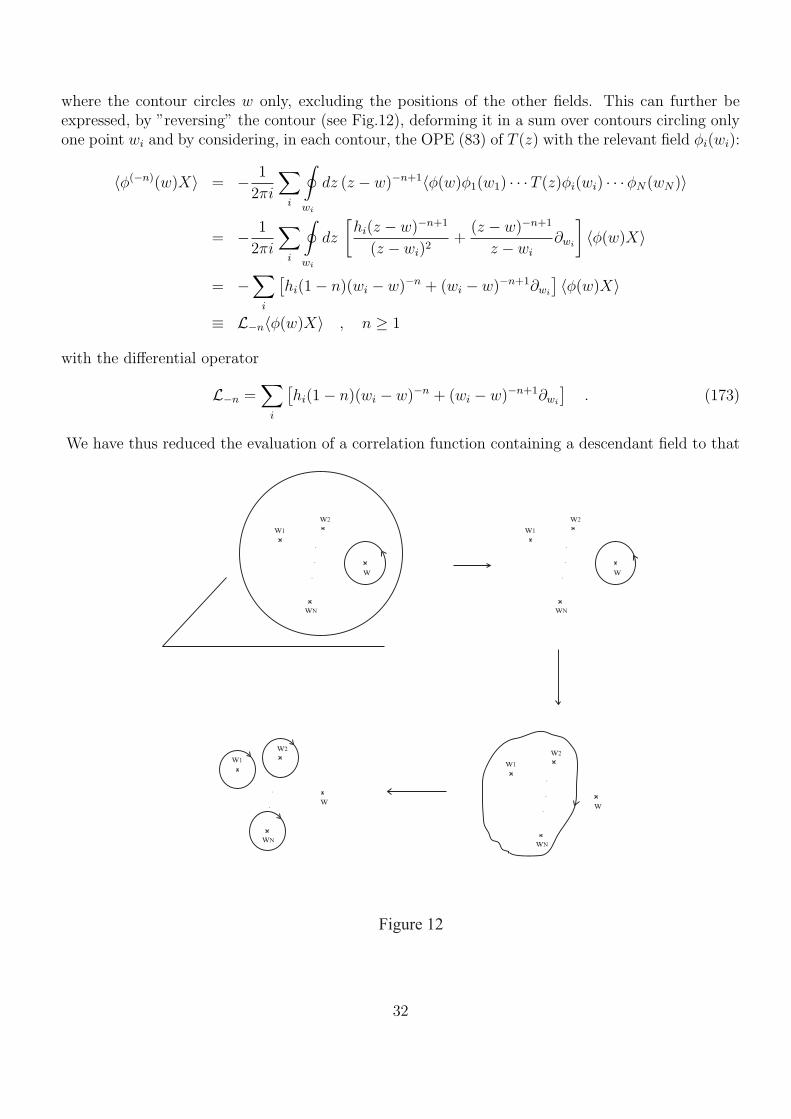
where the contour circles w only, excluding the positions of the other fields. This can further beexpressed, by ”reversing” the contour (see Fig.12), deforming it in a sum over contours circling onlyone point wi and by considering, in each contour, the OPE (83) of T (z) with the relevant field φi(wi):

〈φ(−n)(w)X〉 = − 1

2πi

∑i

∮

wi

dz (z − w)−n+1〈φ(w)φ1(w1) · · ·T (z)φi(wi) · · ·φN(wN)〉

= − 1

2πi

∑i

∮

wi

dz

[hi(z − w)−n+1

(z − wi)2+

(z − w)−n+1

z − wi

∂wi

]〈φ(w)X〉

= −∑

i

[hi(1− n)(wi − w)−n + (wi − w)−n+1∂wi

] 〈φ(w)X〉

≡ L−n〈φ(w)X〉 , n ≥ 1

with the differential operator

L−n =∑

i

[hi(1− n)(wi − w)−n + (wi − w)−n+1∂wi

]. (173)

We have thus reduced the evaluation of a correlation function containing a descendant field to that

w1

w2

w

wN

.

.

.

w1

w2

w

wN

.

.

.

w1

w2

w

wN

.

.

.

w1

w2

w

wN

.

.

.

Figure 12

32

of a correlator of primary fields, on which we must apply a differential operator. Because

(∂w +∑

i

∂wi)〈φ(w)X〉 = 0 (174)

for any correlator as a consequence of translation invariance (see (150) and (152) for i = −1) andL−1 = −∑

i ∂wi, we have

L−1〈φ(w)X〉 = ∂w〈φ(w)X〉 = 0 . (175)

A general descendant field, corresponding to the state (139), has the form

φ(−k1,··· ,κN )(w)4= (L−k1 · · ·L−kN

φ)(w) . (176)

These field are defined recursively, for instance

φ(−k,−n)(w) = (L−kL−nφ)(w)

=1

2πi

∮

w

dz (z − w)1−kT (z)(L−nφ)(w) , (177)

and so on. In particular,

φ(0,−n)(w) = (h + n)φ(−n)(w) and φ(−1,−n)(w) = ∂wφ(−n)(w) . (178)

The first relation is clear from the Virasoro algebra:

φ(0,−n)(w) = (L0L−nφ)(w) = (L−nL0φ)(w) + n(L−nφ)(w) = (h + n)(L−nφ)(w) . (179)

The second expresses the transformation of the fields under translations. The variation of φ(−n)(w)under translations (z−→z + α−1, Φ(z)−→Φ′(z′) = Φ(z)) is given by

δα−1φ(−n)(w) = −α−1∂φ(−n)(w) (180)

as for any field. This can also be expressed from (122) and (119), for n = −1 :

δα−1φ(−n)(w) = − 1

2πiα−1

∮

z

dw T (w)φ(−n)(w) . (181)

But the r.h.s. of (181) is just −α−1φ(−1,−n)(w), see (177), and thus with (180) we find the second

relation.Finally, it can be shown that

〈φ(−k1,··· ,κN )(w)X〉 = L−k1 · · · L−kN〈φ(w)X〉 , (182)

that is, we simply need to apply the differential operators in succession. We may also consider corre-lators containing more than one descendant field, but at the end the result is the same : correlationfunctions of descendant fields may be reduced to correlation functions of primary fields. This is whyprimary fields are of prime interest in CFT’s.The set comprising a primary field φ and all of its descendants is called a conformal family, and isdenoted by

[φ] = {φ, (L−nφ), · · · , (L−k1 · · ·L−kN)} , n > 0, ki > 0 . (183)

The members of a family transform amongst themselves under a conformal transformation. Thismeans that the OPE of T (z) (which generates conformal transformations , see (106), (120)) withany member of the family will be composed solely of other members of the same family (conformalfields have an anti-holomorphic part as well, so there will also be descendants of the field throughthe action of the anti-holomorphic generators L−n).

33

4.6 Operator algebra

We have seen in section 4.4 that conformal invariance takes us a step towards solving a givenconformal field theory (i.e. to be able, at least in principle, to write down all correlation functions ofall the fields present in the theory), by completely fixing the coordinate dependence of the two- andthree-point functions. To fix the numerical coefficients Cijk in (162) and to go beyond three-pointfunctions, some additional information is needed (namely the complete OPE of all primary fieldswith each other). Besides conformal invariance, another basic property of two-dimensional CFT’s isthat operator products can be defined for arbitrary pair of fields. That is, there is a closed operatorproduct algebra among all the fields (called the operator algebra in short). The operator involvedis indeed a product in the sense that it is associative. It is expected that this structure is a directconsequence of the fundamental properties of quantum field theory 24 (see e.g. [8] p. 21), but areusually postulates the existence of the operator algebra as a separate input (this is called the bootstrapapproach, where the set of OPE’s is treated as the fundamental information of the theory, for whichthe whole theory can be reconstructed ). In general, the operator algebra is expressed as

Oi(x) Oj(y) =∑

k

Cijk(x− y) Ok(y), (184)

where the sum runs over all fields present in the theory. (184) is to be understood as constraints oncorrelations functions. In particular, if φ(y) is some field in the QFT,

〈φ(z)Oi(x) Oj(y)〉 =∑

k

Ckij(x− y) 〈φ(z)Ok(y)〉 , (185)

and hence (184) allows to compute all correlation functions of the theory recursively, reducing ulti-mately to the 2-point functions, which are known. Let us make this more precise. We have seen thatthe 2-point function vanishes if the conformal dimensions of the two fields are different (161). Weare free to choose a basis of primary fields such that

〈φ1(w, w)φ2(z, z)〉 =

{ 1(w−z)2h(w−z)2h if h1 = h2 = h and h1 = h2 = h ,

0 otherwise .(186)

it is a simple matter of normalization.

Thus, primary fields φ1 and φ2 with different conformal dimensions are orthogonal in the sense ofthe two-point functions. This is also the case for all the descendants fields of φ1 and φ2, because aswe have seen in section 4.5, correlation functions of descendant fields can be reduced to correlationfunctions of primary fields. Thus, if h1 6= h2, then the conformal families [φ1] and [φ2] are orthogonal

(〈φ(−n1,...,−nh)1 φ

−l1,...,−ln)2 〉 = 0 if h1 6= h2). The same is true for the corresponding Verma modules.

Let

24A heuristic argument goes as follows . According to the OPE assumption, in any QFT, the product of localoperators acting at points that are sufficiently close to each other may be expanded in terms of the local fields of thetheory: φi(x)φj(y)

∑k Cij

k(x−y)φk(y), where Cijk(x−y) are (possibly singular for x → y) functions. This is usually

an asymptotic statement in QFT. In QFT though it is believe it becomes an exact statement because scale invariance(dilatations) prevents the appearance of any length l in the theory. So, there is no parameter to control the expansion,and thus no terms like el(x−y) which would the breakdown of the exactness of the asymptotic expansion above.

34

|h1, h1〉 = φ1(0, 0)|0〉 (187)

|h2, h2〉 = φ2(0, 0)|0〉, (188)

see (126). Then

〈h1, h1|h2, h2〉 = limz,z,w,w→0

〈0|φ+1 (z, z)φ2(w, w)|0〉

= limz,z,w,w→0

z−2h1z−2h1〈0|φ1(1

z

1

z)φ2(w, w)|0〉

= limρ,ρ→0

ρ2h1ρ2h1〈0|φ1(ρ, ρ)φ2(0, 0)|0〉

=

{1 if h1 = h2 = h ,

0 if h1 6= h1 .(189)

using (186).This is also evident from the fact that two eigenspaces of a Hermitian operator (here L0) having differ-ent eigenvalues are orthogonal. Furthermore, the othogonality of the h.w.s. implies the othogonalityof the Verma modules associated to the two fields (this is also as consequence of the orthogonalityof the conformal families, because descendant states can be seen as created for the vacuum by theapplication of the descendant fields, see (165)). The operator algebra takes the general form

φ1(z1, z2)φ2(0, 0) =∑

p

Cp12 zhp−h1−h2 zhp−h1−h2 × [φp(0, 0) + zβ(−1)

p φ(−1)p (0, 0) + zβ

¯(−1)p φ

¯(−1)p (0, 0)

+zzβ(−1)p β

¯(−1)p φ(−1,−1)

p (0, 0) + z2(β(−1,1)p φ(−1,1)

p (0, 0) + β(−2)p φ(−2)

p (0, 0))

+z2(...) + ...] (190)

where the sum runs over all conformal dimensions present in the theory, φ(−1)p = (L−1φp), φ

¯(−1)p =

(L−1φp), φ(−1) ¯(−1)p = (L−1L−1φp), ... as usual, and the coefficients βp are constants defining how the

descendants of a given family [φp] contribute to the OPE, which can be determined as functionsof the central charge and of the conformal dimensions by requiring that both sides of (190) behaveidentically upon conformal transformations (for an example of such a computation, see [2] p. 181and [1] p. 51).

We now focus on the z-part of (190):

φ1(z)φ2(0) =∑

p

Cp12z

hp−h1−h2 [φp(0) + zβ(−1)p φ(−1)

p (0) + z2(β(−1,1)p φ(−1,1)

p (0) + β(−2)φ(−2)p (0)) + ...(191)

The prefactor zhp−h1−h2 ensures invariance under scaling transformations. Indeed, consider z →λz, φ(z) → φ′(z′) = λ−hφ(z). Applying this to both sides, we have for the l.h.s. :

φ1(z)φ2(0) → λ−h1−h2φ1(z)φ2(0), (192)

while for the first term on the r.h.s.:

35

zhp−h1−h2φp(0) → λ−h1−h2 λhp zhp−h1−h2 λ−hp φp(0). (193)

Thus both sides get multiplied by the same factor λ−h1−h2 . For the descending fields, one needsadditional factors, because L0φ

(−1)p = φ

(0,−1)p = (hp +1)φ

(−1)p , see (178), which translates into the fact

that φ(−1)p (w) transforms under dilations (L0) as a primary field of conformal dimension (hp +1). So,

zhp−h1−h2zφ(−1)p (0) → λhp+1λ−h1−h2λ−hp−1φ(−1)

p (0), (194)

and so on for the other descendants at higher levels.In conclusion, the complete operator algebra may be deduced form the conformal symmetry, theonly necessary ingredients being the central charge, the conformal dimensions of the primary fieldsand the coefficients Ck

ij. The latter can be obtained from another source, through a procedure calledthe conformal bootstrap, consisting essentially in implementing the constraint of associativity ofthe operator product algebra (crossing symmetry) (see [2]Sections 6.6.4 and 6.6.5,[3] p49,[7] p16,[8]p42,[9] p22). Thus, any n-point function can in principle be calculated from the operator algebra bysuccessive reduction of the products of primary fields. The correlations of descendant fields obtainedcan be expressed in terms of primary field correlators, and so on, up to two-point functions whichare known. So the theory is solved, in principle!

4.7 Ward identities: final chapter

We discussed Ward identities at different places in these notes, using two different formalisms ofquantum field theory. Within the path integral representation, we found that the variation of acorrelation function 〈φ(x1)...φ(xn)〉 = 〈X〉 under an arbitrary conformal transformation z → z +α(z), φ(z) → φ′(z + α(z)) is given by

δα〈X〉 = − 1

2πi

∮

C

dξα(ξ)〈T (ξ)X〉 (195)

where C encircles the position of all fields in X. On the other side, in the operator formalism, weobserved in section 4.4 that for α(z) corresponding to a global conformal transformation

αg(z) = α−1 + α0z + α−1z2 , (196)

this variation vanishes:

δαg〈X〉 = 0. (197)

We would now like to verify that (195) effectively vanishes for α(z) of the form (196). This maybe done using the operator algebra (191). Let us work out explicitly a simple example. Considerthe case X = φ1(z1)φ2(0). This product can be expanded using (191). Now, recall from (169) thatT (z) belongs to the family of the identity operator I (with h = 0), and that conformal familiescorresponding to different primary fields are orthogonal. Thus, when considering 〈T (ξ)φ1(z1)φ2(0)〉and expanding φ1(z1)φ(0) using (191), the only family involved in the expansion will be that of theidentity operator (which is the only (one) primary field with h = 0). Then,

36

〈T (ξ)X〉 = 〈T (ξ)z−h1−h21 (I + z1β

−10 I(−1)(0) + z2

1(β(−1,−1)0 I(−1,−1)(0) + β

(−2)0 I(−2)(0)) + ...) (198)

But, from (232), we know that 〈T (ξ)〉 = 0, and I(−1) = (L−1I) = 0, because the vacuum is SL(2,C)invariant (L−1|0〉 = 0). We have, because I(−n)(w) = 1

(n−2)!∂(n−2)T (w), see (165),

〈T (ξ)X〉 = z−h1−h2+21 〈T (ξ)T (0)〉β−2

0 + terms involving〈T (ξ)∂nT (0)〉, n ≥ 1 (199)

In (195), note that we can send the contour (to infinity, because all operators are already inside C.This way, the integrand behaves as

α(ξ)〈T (ξ)X〉 ∼ξ→∞

α(ξ)〈T (ξ)T (0)〉 ∝ α(ξ)

ξ4, (200)

where we used (233). Thus for α(ξ) given by (196), the integral in (195) vanishes. We recover the in-variance of 〈X〉 w.r.t. to transformations of the global conformal group. For local transformations itis relation (195) that holds, instead of the expected invariance. Returning to the derivation of sec-tion 4.4, we may see that this originates from the apparition of the central charge c, which preventsto apply the same procedure, because we don’t have 〈0|Ln = Ln|0〉 ∀n, but only for i = −1, 0, 1corresponding to the global subgroup.

4.8 A short story on normal ordering

In this section, I will introduce the notion of conformal normal ordering, and show that it reducesin some situations to the more familiar operator normal ordering, consisting in moving annihilatoroperators to the right. We saw that the OPE of two fields can be written in general as

A(z)B(w) =N∑

n=−∞

{AB}n(w)

(z − w)n(201)

The conformal normal ordering of the two fields, denoted by :AB: , is by definition

:AB: (w)4= {AB}0(w), (202)

that is, the term of order (z − w)0 in the OPE. This is a particular prescription, which in generaldiffers from the definition

:AmBn: =

{AmBn for n > 0 ,

BnAm for n ≤ 0 .(203)

where

37

Am := Am(0) =1

2πi

∫dzzm+hA−1A(z)

Bn :=1

2πi

∫dzzm+hB−1B(z) (204)

are the modes of the fields A(z) and B(z) (see (115)). We will return to this.

The singular terms in an operator product are called contraction and are denoted by

A(z)B(w)4=

N∑n=1

{AB}n(w)

(z − w)n. (205)

Again this definition is in general different from the QFT one, where contraction generally meanspropagator (two-point function).This is well illustrated in the case of the field T (z). Indeed, with (205) and (96), one has

T (z)T (w) =c/2

(z − w)4+

2T (w)

(z − w)2+

∂T (w)

(z − w), , (206)

while

〈T (z)T (w)〉 =c/2

(z − w)4. (207)

From (202), the conformal normal ordering can be represented using contour integration by

:AB: (w) =1

2πi

∫dz

(z − w)A(z)B(w) (208)

where, as usual radial ordering is understood in the r.h.s.

The OPE (201) is then

A(z)B(w) = A(z)B(w) + :AB: (w) + O(z − w) (209)

Notice that, when the contraction coincides with the propagator, this formula is exactly the onewe get in usual QFT, where the ordering is the familiar operator normal ordering (203). A fieldfor which the contraction contains only one singular term (necessarily coinciding with the 2-pointfunction) is called a free field. In this situation, both orderings are equivalent, and Wick’s theoremmay be applied as such. When the field are not free, Wick’s theorem must be adapted (see [2] p188).

38

5 The free boson

Consider the following action for a massless scalar field in two dimensions

S =1

8π

∫d2x ∂µφ∂µφ , (210)

or in the usual complex coordinates z = x1 + ix2, ∂ = ∂z, · · · :

S =1

4π

∫d2z ∂φ∂φ , (211)

where d2z = dzdz = 2dx1dx2. This action is invariant under scalings x−→λx, φ(x)−→φ′(x′) =λ−∆φ(x) if ∆ = 0.The equations of motion are

δS

δφ= 0 ⇒ ∂∂φ(z, z) = 0 . (212)

The energy-momentum tensor (see (49)) is given by

Tµν =1

4π(∂µφ∂νφ− 1

2gµν∂αφ∂αφ) (213)

and thus (gzz = 1/2, gzz = gzz = 0)

Tzz =1

4π∂φ∂φ , Tzz =

1

4π∂φ∂φ (214)

Later on we will use the following convenient normalization

T (z) = −2πTzz , T (z) = −2πTzz . (215)

The primary input we need is the OPE of the fields appearing in the action. This can be obtainedby the following method. Consider the variation

δφ(x) = ε(x) (216)

and its effect on correlation functions of the form 〈φ(x1) · · ·φ(xN)〉 4= 〈X〉. The variation of 〈X〉 isgiven by (46), with

δS =1

4π

∫d2x∂µε∂

µφ . (217)

Thus, we have

∑i

ε(xi)〈φ(x1) · · · ˆφ(xi) · · ·φ(xN)〉 =1

4π

∫d2x ∂µε(x)∂µ〈φ(x)X〉 , (218)

whereˆstands for omission. Integrating the r.h.s. by parts and discarding the boundary term, onehas

− 1

4π

∫d2x ε(x)∂µ∂

µ|x 〈φ(x)X〉 . (219)

39

Therefore, (218) implies that

− 1

4π2x〈φ(x)X〉 =

∑i

δ2(x− xi) 〈φ(x1) · · · ˆφ(xi) · · ·φ(xN)〉 . (220)

This can be solved as

〈φ(x)X〉 =∑

i

ln |z − zi|−2〈φ(x1) · · · ˆφ(xi) · · ·φ(xN)〉+ 〈 :φ(x)φ(x1) · · ·φ(xN): 〉 , (221)

where |z − w|2 = (z − w)(z − w). This is understood as follows. The first term originates from thefact that 2x = 4∂∂ and that

∂∂ ln |z − w|−2 = −πδ2(x− y) , (222)

x = (z, z), y = (w, w) and∫

d2x δ2(x)f(z) = f(0). Eq. (222) follows from the following representa-tion of the δ function :

δ2(x) =1

π∂z

1

z=

1

π∂z

1

z, (223)

see e.g. [2] p.119. The second term of the r.h.s. of (221) actually defines :φ(x)φ(x1) · · ·φ(xN): ,where the function 〈 :φ(x)φ(x1) · · ·φ(xN): 〉 satisfies

∂∂〈 :φ(x)φ(x1) · · ·φ(xN): 〉 = 0 , (224)

i.e. it is a harmonic function. It is thus locally the sum of an analytic and anti-analytic function,and can be Taylor expanded. In particular, it has no pole as x→xi. Eq. (221) gives us the behaviorof the function 〈φ(x)φ(x1) · · ·φ(xN)〉 as x→xi, i.e. by definition the OPE of φ(x) with itself. This iswritten

φ(z, z)φ(zi, zi) ∼ ln |z − zi|−2 , (225)

where this relation is to be understood inside a correlation function with other fields, and ∼ meansequality modulo terms regular as x→xi. If there are no other fields, this gives us the propagator

〈φ(z, z)φ(zi, zi)〉 = ln |z − zi|−2 , (226)

up to a harmonic function (regular as z→zi). This shows, as expected, that φ(z, z) is a free field, asdefined in the preceding section.Finally, eq. (221) is usually rewritten as

φ(z, z)φ(zi, zi) = ln |z − zi|−2 + :φ(z, z)φ(zi, zi):= 〈φ(z, z)φ(zi, zi)〉+ :φ(z, z)φ(zi, zi): , (227)

which is the familiar relation between time(radial)-ordering and normal ordering in QFT.This can be brought in the form (209) by Taylor expanding the whole series of regular terms:φ(z, z)φ(zi, zi): as

:φ(z, z)φ(zi, zi): = :φφ: (zi, zi) + (z − zi) :∂φ φ: (zi, zi) + (z − zi) :∂φφ: (zi, zi) + · · · , (228)

from which we deduce

φ(z, z)φ(zi, zi) = ln |z − zi|−2 + :φφ: (zi, zi) + (z − zi) :∂φ φ: (zi, zi) + (z − zi) :∂φ φ: (zi, zi) + · · · .(229)

40

Focusing on the z sector, we are left with

φ(z)φ(w) = − ln(z − w) + :φφ: (w) + (z − w) :∂φ φ: (w) + · · · , (230)

which coincides exactly with (209). We may also write

:φφ: (w, w) = limz,z→w,w

[φ(z, z)φ(w, w)− 〈φ(z, z)φ(w, w)〉] (231)

6 Exercises

6.1 Operator formalism

1. Show that (144) implies that〈T (z)〉 = 〈 0 |T (z)| 0 〉 = 0 (232)

2. Compute the two-point function of T (z) and show that

〈T (z)T (w)〉 = 〈 0 |T (z)T (w)| 0 〉 =c/2

(z − w)4, (233)

by using (144), (131) and (124).This can also be inferred from (96) and (232)

3. Compute the norm of the state L−2| 0 〉 and show that a necessary condition for the theoryto be unitary is c > 0.

4. Compute the singular part of the OPE of φ(−1)(w) with T (z), and deduce from this the transfor-mation law of the descendant field φ(−1)(w). For this, use the expansion T (z) =

∑k(z−w)−k−2Lk(w)

and the Virasoro algebra (124).

(R : T (z)φ(−1)(w) ∼ 2hφ(w)(z−w)3 + (h + 1)φ(−1)(w)

(z−w)2 + ∂φ(−1)(w)z−w and δα(z)φ

(−1)(z) = −hα′′(z)φ(z)− (h + 1)α′(z)φ(−1)(z)−α(z)∂φ(−1)(z), where h is the conformal weight of the primary field φ(z) from which the field descends.)

6.2 Free boson

1. From (225), write the OPE of ∂zφ(z, z)∂wφ(w, w) and ∂zφ(z, z)∂wφ(w, w).

(R : ∂zφ(z, z)∂wφ(w, w) ∼ − 1(z−w)2 and ∂zφ(z, z)∂wφ(w, w) ∼ − 1

(z−w)2 . Thus everything splits in a holomorphic and

anti-holomorphic part. In the following, we will focus on the holomorphic field ∂φ4= ∂zφ.)

2. The energy-momentum tensor (214) is not well defined because ∂φ(z)∂φ(w) have singularitiesas z→w. Therefore the quantum version of (215) is

T (z) = −1

2:∂φ ∂φ: , T (z) = −1

2:∂φ ∂φ: . (234)

that is, with (231)

T (z) = −2π limw→z

[∂φ(z) ∂φ(w)− 〈∂φ(z, z) ∂φ(w, w)〉] . (235)

41

Compute the OPE T (z)∂φ(w). What does this show? You could need the following Wick’s rules:

T (φ1φ2φ3) = :φ1φ2φ3: + :φ1φ2φ3: + :φ1φ2φ3: + :φ1φ2φ3: , (236)

with similar relations holding when some factors are already normal-ordered in the the T-product,but with omission of contractions inside a same normal ordering. For instance, T ( :φ1φ2: :φ3φ4: )does not contain the term 〈φ1φ2〉 :φ3φ4: .(R : T (z)∂φ(w) ∼ ∂φ(w)

(z−w)2 + ∂2φ(w)z−w )

3. Compute the OPE T (z)T (w). Check it has the form (96) and deduce the central charge ofthe system.

4. Consider the following field, called a vertex operator :

Vα(w) = :eiαφ(w): . (237)

a. Compute its OPE with ∂φ(z)(R: ∂φ(z)Vα(w) ∼ − iα

z−w Vα(w) )b. Compute its OPE with T (z) and show this operator is primary with conformal weight α2/2.

5. Compute the OPE :(∂φ(z))k: :Vα(w): . For this, compute the OPE :Ak: :eB: , for two gen-eral operators A and B.

6. Using the result of Ex.5, show that :eA: :eB: = e〈AB〉 :eA eB: . From this, deduce the corre-lation function 〈Vα(z)Vβ(w)〉 (the correlator being given by the most singular part of the OPE).(R : See [6], p47)

6.3 Ghost system

The b− c ghost system is defined by

1

2π

∫d2x bµν∂

νcν , (238)

where the field bmuν is a traceless symmetric tensor, and where both cµ and bµν are fermions. Goingto complex coordinates, with cz = c, cz = c, bzz = b and bzz = b, the action is rewritten (d2x =12dzdz = 1

2d2z)

1

2π

∫d2z (b∂c + b∂c) . (239)

From the equations of motion the fields c and b are holomorphic. They satisfy the following OPE

b(z)c(w) ∼ 1

z − w. (240)

The normal-ordered holomorphic energy-momentum is obtained as (see e.g. [2], p133)

T (z) = :2∂c b + c ∂b: . (241)

42

1. Compute the OPE’s T (z)c(w) and T (z)b(w). Deduce the conformal weights of c and b.

2. Compute the (most singular part of the) OPE T (z)T (w). What is the central charge of thissystem?

3. This system appears in the covariant quantization of the bosonic string through the gauge-fixing of two dimensional gravity (see [10], Chapter 3). In this context, each space-time coordinateis represented by a free boson. How many free bosons do you need in order for the central charge ofthe system ”D free bosons + ghosts” to vanish? You just found one way of computing the criticaldimension of bosonic string theory.

Acknowledgments

I would like to heartily thank Ph. Spindel for numerous enjoyable, useful (and sometimes lively)discussions on the topics discussed here. I am grateful to Vl. Dotsenko for enlightening correspon-dences. I thank E. Rodrigues Ferreira for a discussion and references on complex functions. Finally,big kisses to S. de Buyl for her help at all stages of this work, including discussions, support (in allsenses), typing part of these notes, etc. etc!

Appendix A : Another derivation of the conformal Ward

identities

This section is mainly based on [2]. Therefore I won’t go through all calculations in details, sincethey may be found in the reference.Let us start with an action S[φ] =

∫ddxL(φ(x), φ,µ(x)), and consider the following infinitesimal

transformations

xµ −→ x′µ = xµ + ωa δxµ

δωa, (242)

φ(x) −→ φ′(x′) = φ(x) + ωa δFδωa

(x) . (243)

which are supposed to leave the action S invariant when the infinitesimal parameters {ωa} areconstant (the subscript ”a” indicating as before a collection of indices). Noether’s theorem statesthat to every continuous symmetry of a field theory corresponds a conserved current, and hence aconserved charge. To determine this current, one may use the ”Noether’s trick”, which consists inlooking at the variation of the action under the same transformation, but with ωa depending onthe position. This doesn’t leave the action invariant anymore, and the variation may be written ingeneral as

S ′ = S + terms involving derivatives of ωa(x) + terms without derivatives of ωa(x) . (244)

Because S ′ = S when the ωa’s are constants, the last contributions must sum up to zero. Then thevariation of the action can be found to be

δS =

∫ddx jµ

a ∂µωa , (245)

43

with

jµa =

{∂L

∂(∂µφ)∂νφ− δµ

ν L

}δxν

δωa− ∂L

∂(∂µφ)

δFδωa

. (246)

If ωa(x)→0 at infinity, this relation can be integrated by parts, to yield

δS =

∫ddx ∂µj

µa ωa . (247)

Now, if the field configuration satisfies the classical equations of motion, the action is stationaryagainst any variation of the fields, and δS should vanish for any position-dependent parametersωa(x). This implies

∂µjµa ≈ 0 . (248)

This is Noether’s theorem : every continuous symmetry implies the existence of a current, conservedon-shell.We may now return to the Ward identity in field theory. We follow the same procedure which led usto (46). In the path integral, we make the following change of variable :

φ(x)−→φ′(x) = φ(x)− iωa(x)Gaφ(x) , (249)

where the parameters depend on x, and hence δS is not 0 and given by (247). Notice that thevariation of a field is here defined by δφ(x) = −iωaGaφ(x) and differs from (13) by a factor −i. Wekeep this factor to be coherent with [2] but it is unimportant. We may now rewrite (46) using (247)and (249) as

−i

n∑i=1

ωa(xi)〈φ1 · · ·Gaφi · · ·φn〉 =

∫ddxωa(x) ∂µ〈jµ

a (x)φ1 · · ·φn〉 , (250)

where ωa(x) are arbitrary functions. In the l.h.s., only the values of ωa(xi), i = 1, · · · , n matter.This equation is thus of the form

∫f(x)h(x)dx = f(y)φ(y)∀f(x), which necessarily implies h(x) =

φ(x)δ(x− y). From (250), we thus conclude that

∂µ〈jµa (x)φ1(x1) · · ·φn(xn)〉 = −i

n∑j=1

δ(x− xj)〈φ1 · · ·Gaφj(xj) · · ·φn〉 . (251)

This is the Ward identity for the current jµa . Applying this to translations, we find from (246) that

jµν = −ηµνL +∂l

∂(∂µφ)∂νφ

4= T µν

c , (252)

and recover the fact that the conserved current associated to translation invariance is the canonicalenergy-momentum tensor. This also shows that the energy-momentum tensor is conserved insidecorrelation functions except at coincident points.Notice that the form of the current may be modified from its canonical definition (246) withoutaffecting the Ward identity. We may indeed freely add to it the divergence of an antisymmetric tensorwithout affecting its conservation. In the case of a system invariant under Lorentz transformations(rotations), it can be shown that there always exist an antisymmetric tensor Bµνρ, with Bρµν = −Bµρν

such that the tensorT µν

B

4= T µν

c + ∂ρBρµν (253)

44

is symmetric on-shell, that is T[µν]B ≈ 0. This new tensor is called the Belinfante tensor (see [2]p46 for

its construction). Furthermore, much in the same way, the energy-momentum tensor of a theory withscale invariance can be made traceless on-shell, under certain certain conditions which are generallyassumed to be fulfilled (see [2] p.102). By using this suitably modified energy-momentum tensor, theWard identities associated with translation, rotation and dilation invariance can be obtained from(251). In two dimensions, the result is (see [2] p106,118,123)

∂µ〈T µν (x)X〉 = −

n∑i=1

δ(x− xi)∂xνi〈X〉 (254)

εµν〈T µν(x)X〉 = −i

n∑i=1

siδ(x− xi)〈X〉 (255)

〈T µµ (x)X〉 = −

n∑i=1

∆iδ(x− xi)〈X〉 (256)

Here X stands for a string of primary fields. In two dimensions, the spin generators are given bySµν = sεµν , and ∆ stands for the scaling dimensions of the fields. These relations show that, insidecorrelations functions, the energy-momentum tensor is conserved, symmetric and traceless, exceptat coincident points. This is the quantum counterpart of the classical statement that the energy-momentum tensor is conserved, symmetric and traceless on-shell. A derivation of these identitieswhich does not require the hypothesis that the energy-momentum can be made classically tracelesscan be found in [2], p123.We may now turn to the conformal Ward identity. Let εµ(x) be (the components of) a conformalKilling vector, satisfying (11), and defining an infinitesimal conformal transformation. We may write

∂µ(ενTµν) = εν∂µT

µν +1

2(∂µεν + ∂νεµ)T µν +

1

2(∂µεν − ∂νεµ)T µν (257)

= εν∂µTµν +

1

2(∂ρε

ρ)T µµ +

1

2εαβ∂αεβεµνT

µν , (258)

where we used

1

2(∂µεν + ∂νεµ) =

1

2(∂ρε

ρ)ηµν (259)

1

2(∂µεν − ∂νεµ) =

1

2εαβ∂αεβεµν . (260)

Remark that ∂µ(ενTµν) ≈ 0, therefore ενT

µν is sometimes called the conformal current. Let uscompute ∫

M

d2x ∂µ〈εν(x)T µν(x)X〉 , (261)

where M is a domain including all insertion points xi. We will also assume that inside this domain,the functions ε(z) and ε(z) have no singularities (this can always be realized if ε and ε are regular atx = xi). By using (258) and eqs. (254) to (256), as well as εzz = −2i, hi = 1

2(∆i+si), hi = 1

2(∆i−si),

we get, using complex coordinates∫

M

d2x ∂µ〈εν(x)T µν(x)X〉 = −∑

i

(ε(zi)∂zi+ ε(zi)∂zi

+ hi∂ziε(zi) + hi∂zi

ε(zi))〈X〉

4= δε,ε〈X〉 , (262)

45

where εz = ε(z), εz = ε(z). The l.h.s. can further be expanded with the relation∫

Md2x ∂µF

µ =i2

∫∂M

[−dzF z + dzF z], applied to F µ = εν(x)T µν(x). The fact that T µν is conserved, symmetric andtraceless except at coincident points implies that

Tzz(z, z) = Tzz(z)4= − 1

2πT (z) (263)

Tzz(z, z) = Tzz(z)4= − 1

2πT (z) (264)

Tzz(z, z) = Tzz(z, z) = 0 , for (z, z) 6= (zi, zi) , (265)

so that (262) finally reduces, because the domain M strictly contains all insertion points (and so thecontour C = ∂M does not go through the insertion points), to

δε,ε〈X〉 = − 1

2πi

∮

C

dwε(w)〈T (w)X 〉+1

2πi

∮

C

dwε(w)〈T (w)X 〉 . (266)

In deriving this relation, we have used the property that the fields in the set X are primary, throughthe Ward identities (254)-(256) (see their derivation p123 of [2]). However, eq. (266) may be taken asa definition of the effect of conformal transformations on an arbitrary local field within a correlationfunction, see [2], p122.

References

[1] Vl. Dotsenko, Serie de Cours sur la Theorie Conforme, http://cel.ccsd.cnrs.fr/cours/cel-2/cel-2.html

[2] Ph. Di Francesco, P. Mathieu, D. Senechal, Conformal Field Theory, Springer

[3] A.N. Schellekens , Introduction to conformal field theory, Fortsch. Phys, 1996, http://staff.science.uva.nl/~jdeboer/stringtheory/CFT.ps

[4] Y. Saint-Aubin, Phenomenes critiques en deux dimensions et invariance conforme, LectureNotes, Universite de Montreal (1987)

[5] E. Kiritsis,Introduction to Superstring Theory,hep-th/9709062

[6] C.J. Efthimiou, D.A. Spector, A Collection of Exercises in Two-Dimensional Physics, Part 1,hep-th/0003190

[7] J. Fuchs, Lectures on conformal field theory and Kac-Moody algebras, hep-th/9702194

[8] P.Ginsparg, Applied Conformal Field Theory, in “Fields, Strings and Critical Phenomena, (LesHouches, Session XLIX, 1988) ed. by E. Brezin and J. Zinn Justin, 1989”, hep-th/9108028

[9] J. Bagger, Basic Conformal Field Theory, http://ccdb3fs.kek.jp/cgi-bin/img\_index?

200031975

[10] M.Green,J.Schwartz, E. Witten, Superstring theory, Cambridge University Press, 1987

[11] J.Polchinsky, String theory, Vol.1 ,Cambridge Univ. Pr. (1998)

46