asphaltene precipitation modeling in dead crude oils using

Vol.:(0123456789)1 3

Journal of Petroleum Exploration and Production Technology (2021) 11:3599–3614 https://doi.org/10.1007/s13202-021-01233-y

ORIGINAL PAPER-PRODUCTION ENGINEERING

Asphaltene precipitation modeling in dead crude oils using scaling equations and non‑scaling models: comparative study

Syed Imran Ali1 · Shaine Mohammadali Lalji1 · Javed Haneef1 · Clifford Louis2 · Abdus Saboor1 · Nimra Yousaf1

Received: 20 May 2021 / Accepted: 6 July 2021 / Published online: 7 August 2021 © The Author(s) 2021

AbstractThis research study aims to conduct a comparative performance analysis of different scaling equations and non-scaling models used for modeling asphaltene precipitation. The experimental data used to carry out this study are taken from the published literature. Five scaling equations which include Rassamadana et al., Rassamdana and Sahimi, Hu and Gou, Ashoori et al., and log–log scaling equations were used and applied in two ways, i.e., on full dataset and partial datasets. Partial datasets are developed by splitting the full dataset in terms of Dilution ratio (R) between oil and precipitant. It was found that all scaling equations predict asphaltene weight percentage with reasonable accuracy (except Ashoori et al. scaling equation for full dataset) and their performance is further enhanced when applied on partial datasets. For the prediction of Critical dilu-tion ratio (Rc) for different precipitants to detect asphaltene precipitation onset point, all scaling equations (except Ashoori et scaling equation when applied on partial datasets) are either unable to predict or produce results with significant error. Finally, results of scaling equations are compared with non-scaling model predictions which include PC-Saft, Flory–Huggins, and solid models. It was found that all scaling equations (except Ashoori et al. scaling equation for full dataset) either yield almost the same or improved results for asphaltene weight percentage when compared to best case (PC-Saft). However, for the prediction of Rc, Ashoori et al. scaling equation predicts more accurate results as compared to other non-scaling models.

Keywords Scaling equations · Non-scaling models · Asphaltene precipitation · Modeling · Performance · Dilution ratio

AbbreviationsR Dilution ratioRc Critical dilution ratioSARA Saturates, aromatics, resins, and

asphaltenesASTM American society for testing and

materialsEoS Equation of stateM Molecular weight of precipitantWt% The precipitated asphaltene weight

percentX and Y or x and y Scaling equation variablesXc Value of X at onset point

r1, r2, c1, c2, n Scaling equations adjustable parameters

T TemperatureR2 Coefficient of determinationMAE Mean Absolute ErrorA1, A2, A3, A4 Scaling equation coefficients

Introduction

Crude oil is composed of mainly four components, i.e., saturates, aromatics, resins, and asphaltenes (SARA) (Ashoori et al. 2017). Among all of them, asphaltene is regarded as the heaviest and the most polar constituent of crude oil (Mohammed et al. 2021). Under favorable condi-tions, asphaltene remains as a dissolved entity in crude oils. Crude oils when suffering changes in their composition, due to variation of pressure and temperature conditions, cause asphaltenes to precipitate out and deposit (Gharbi et al. 2017). This problematic situation offers severe challenges to operating companies in terms of preventing hydrocar-bon production shutdowns and applying costly treatment

* Syed Imran Ali [email protected]

1 Department of Petroleum Engineering, NED University Of Engineering & Technology, Karachi, Pakistan

2 Department of Chemical and Petroleum Engineering, University of Calgary, 2500 University Drive NW, Calgary, AB, Canada

http://orcid.org/0000-0003-0133-9455

http://crossmark.crossref.org/dialog/?doi=10.1007/s13202-021-01233-y&domain=pdf

3600 Journal of Petroleum Exploration and Production Technology (2021) 11:3599–3614

1 3

methods (Melendez-Alvarez et al. 2016). Therefore, this scenario makes it necessary for operators to predict the con-ditions and extent of asphaltene precipitation of a particular crude oil.

In past, various experimental techniques were applied to determine the amount of asphaltene precipitation from crude oils under different conditions (Zendehboudi et al. 2014). These experimental techniques include standard tests such as IP-143, ASTM D-3279-07, ASTM D-4124-01, ASTM D-4124-09, ASTM D-6560-00, and ASTM D-2007-03 for dead oil (Zheng et al. 2020) and filtration test for live oil (Firoozinia et al. 2016). Apart from these experimental methods, several models have also being developed for the estimation of asphaltene precipitates at different operational conditions and found to complement well with experimental results. According to Mohammadi et al. (Mohammadi et al. 2012), there are five major categories of asphaltene precipi-tation modeling which include: Equation of State (EoS)-based models, ‘Association’ models, colloidal/micellization models, ‘Activity coefficient’-based models, and scaling laws, corresponding states and correlations.

EoS models have been applied extensively for asphaltene precipitation modeling and were found easy to implement due to their availability in commercial software (Zhang et al. 2012; Zendehboudi et al. 2013; Panuganti et al. 2012; Alhosani and Daraboina 2020). These commercial soft-ware include PVTsim of Calsep, Multiflash of infochem, VLXE of VLXE Aps, and Winprop of CMG (Ali et al. 2021).Cubic, Cubic plus association, Saft, and PC-Saft are the well-renowned EoS models (Subramanian et al. 2016). One of the drawbacks of EoS models is that they require fluid characterization normally up to C30+. Moreover, this modeling class sometimes encounters convergence issues especially when polydispersity of asphaltene particle is con-sidered (Mohammadi et al. 2012). Activity coefficient-based models are generally based on the polymer solution or regu-lar solution theories of Flory–Huggins, Scatchard–Hilde-brand, and Scott–Magat model (Subramanian et al. 2016). The mean asphaltene molecular weight is a necessary input for this modeling type. When polydispersity of asphaltene particles is considered, then more tuning parameters are needed (Mohammadi et al. 2012). Furthermore, a suitable distribution function should be utilized in the model. Select-ing an appropriate distribution function is a challenging task and may cause some problems in calculations (Mohammadi et al. 2012). Agrawala and Yarranton introduced an associa-tion model for asphaltene precipitation modeling by con-sidering asphaltene aggregation like linear polymerization (Agrawala and Yarranton 2001). According to the associa-tion model, asphaltene monomers are regarded as propaga-tors, while resin molecules are considered as terminators of polymerization reaction (Agrawala and Yarranton 2001). Leontaritis and Mansoori proposed a colloidal model in

which they considered that resins are attached to the sur-face of asphaltenes and prevent asphaltene precipitation (Leontaritis and Mansoori 1987). The colloidal model can-not estimate the amount of asphaltene precipitation and only be used to predict asphaltene precipitation onset conditions. Victorov and Firoozabadi considered the asphaltene micel-lar and aggregation nature and proposed a thermodynamic micellization model in which resins stabilized asphaltene micelles (Victorov and Firoozabadi 1996). The model is dif-ficult to implement as it contains several adjustable param-eters and requires information about crude oil resin contents (Mohammadi et al. 2012). The last modeling type is the scaling equations. The scaling equations were originally developed on the idea of Park and Mansoori, who studied the similarities between the asphaltene precipitation and aggre-gation/gelation mechanisms (Moghadasi 2019). Rassamdana et al. proposed the first scaling equation to model asphaltene precipitation in dead oil at isothermal conditions by con-sidering parameters that include dilution ratio of n-alkanes (precipitant) and crude oil and molecular weight of n-alkane (Rassamdana et al. 1996). The advantage of using the scal-ing equation is that it does not require critical properties of asphaltenes. Furthermore, these equations are user-friendly and need comparatively less amount of data (Alimohammadi et al. 2020).

As discussed earlier that the implementation of preven-tive measures to control asphaltene precipitation is highly dependent upon the reliable prediction results obtained through models. Therefore, the accuracy of models is of prime importance in this respect. Apart from asphaltene pre-cipitation during the natural depletion process, the problem could arise in processes like VAPEX in which (n-alkanes) solvents are injected in crude oil for lowering its viscosity during transportation (Alimohammadi et al. 2017). In this research study, a detailed statistical and graphical perfor-mance analysis of five scaling equations that are used to model asphaltene precipitation in dead crude oil is carried out. Motivated with the approach adopted by some investi-gators (Alimohammadi et al. 2020; Ashoori et al. 2003) to apply scaling equation on partial datasets formed by break-ing full dataset in terms of certain dilution ratio between precipitant (n-alkane) and crude oil, therefore, in this study we have applied scaling equations on full dataset and on the partial dataset (by breaking the dataset at a dilution ratio of 5). Accordingly, the accuracies of models are monitored and compared with each other. Furthermore, the advantages and drawbacks of each scaling equation are presented. Finally, the results of the scaling equations are also compared with other non-scaling models.

3601Journal of Petroleum Exploration and Production Technology (2021) 11:3599–3614

1 3

Scaling equations applied in this study

Rassamdana et al. scaling equation

The first scaling equation was developed by Rassamdana et al. (Rassamdana et al. 1996). Rassamdana and cowork-ers estimated the asphaltene precipitation by titrating the crude oils with different precipitants at room pressure and temperature. It was found that dilution ratio (R), molecular weight of precipitant (M), and asphaltene weight percentage (wt%) are in relationship through variables X and Y as given by Eqs. 1 and 2:

Rassamdana et al. suggested the value of 0.25 to z while considered z’ as a universal constant having a value of − 2 independent of crude oil and precipitant type. Yu-Feng Hu et al. (Hu et al. 2000) studied and analyzed the Rassamdana et al. scaling equation model and proposed that the value of z may range from 0.1 to 0.5. The values obtained for X and Y are plotted and best fitting is carried out on a curve represented by Eq. 3 termed as scaling equation.

where X ≥ XcCoefficient values of A1 to A4 can be tuned to any oil

species. Xc is the magnitude of X at the asphaltene onset point. Critical dilution ratio (Rc), which refers to the dilution ratio at which asphaltene precipitation starts, is obtained by finding Xc by placing Y = 0 in Eq. 3. Then, Xc along with corresponding M will be used in Eq. 1 to evaluate corre-sponding Rc.

Temperature‑dependent Rassamdana scaling equation

The scaling equation which was initially developed by Ras-samdana et al. is independent of temperature. To incorporate the effect the temperature, Rassamdana et al. proposed a new scaling equation that takes into account the results of the original Rassamdana scaling model to include the tem-perature effect on asphaltene precipitation (Rassamdana and Sahimi 1996). The new relationships developed are given by Eqs. 4 and 5:

(1)X =R

Mz

(2)Y =wt%

Rz�

(3)Y = A1 + A2X + A3X2 + A4X

3

(4)x =X

Tc1

where X and Y are the variables of temperature-inde-pendent Rassamdana et al. scaling equations. C1 and C2 are the adjustable parameters. Rassamdana et al. found accu-rate estimates of asphaltene precipitation at c1 = 0.25 and c2 = 1.6.

The new proposed scaling model can be expressed in terms of new variables x and y through a third-order poly-nomial equation given by Eq. 6:

where x ≥ xc.A1 to A4 are scaling coefficients and xc is the value of x

at the asphaltene precipitation onset point. Critical dilution ratio (Rc) is determined by finding xc by placing y = 0 in Eq. 6. Then, obtained xc is placed in Eq. 4 to find the cor-responding value of Xc. Finally, the Xc is substituted in Eq. 1 to obtain Rc.

Hu and Guo scaling equation

Hu and Guo (Hu and Guo 2000) proposed a scaling equation to model asphaltene precipitation of Chinese dead crude oil at different temperatures, dilution ratios, and precipitants. It was found that the developed scaling equation yields more accurate results as compared to the Rassamdana et al. scal-ing equation. The new relationships of x and y with experi-ment variables are represented by Eqs. 7 and 8:

where X is the variable of Rassamdana et al. scaling equa-tion while c1, c2, z, and z’ are the adjustable parameters. Hu and Guo found the best estimates of asphaltene precipitation at z = 0.25, z’ = − 2, c1 = 0.5, and c2 = 1.6.

The new proposed scaling model can be expressed in terms of new variables x and y through a third-order poly-nomial equation as Eq. 9:

where x ≥ xc.A1 to A4 are scaling coefficients and xc is the value of x

at the asphaltene precipitation onset point. Critical dilution ratio is determined by finding xc by placing y = 0 in Eq. 9. Then, xc along with other corresponding variables, i.e., M and T, will be used in Eq. 7 to evaluate corresponding Rc.

(5)y =Y

Xc2

(6)y = A1 + A2x + A3x2 + A4x

3

(7)x =R

Tc1Mz

(8)y =wt%

Xc2

(9)y = A1 + A2x + A3x2 + A4x

3


1 3

Ashoori et al. scaling equation

Ashoori et al. (Ashoori et al. 2003) conducted a series of experiments using Iranian dead crude oil at different tem-peratures. They modeled asphaltene precipitation by applying Rassamdana et al. and Yu-Feng Hu et al. scaling equations. As predicted results were not found too accurate by these two models, therefore, Ashoori et al. developed a new scaling equation that produced asphaltene precipitation close to those yields experimentally. They found X and Y in the following relationship as given by Eq. 10 and 11:

where n, z, and z’ are the adjustable parameters. It was pro-posed that n may be taken in between 0.1 and 0.25 while z and z’ as 0.25 and − 2, respectively. Ashoori et al. found accurate results at n = 0.15. The scaling model can be expressed in terms of new variables x and y through a third-order polynomial equation as Eq. 12:

where X ≥ Xc.A1 to A4 are scaling coefficients and Xc is the value of X at

the asphaltene precipitation onset point.Ashoori et al. formed two scaling equations for the calcu-

lation of asphaltene precipitation. One scaling equation was developed by using data up to dilution ratio 7, while the other was constructed utilizing a dilution ratio of more than 7. Xc is determined by using the scaling equation developed by utiliz-ing dataset up to dilution ratio of 7 and further placed in Eq. 10 to find Rc.

Log–log scaling equation

Log–log scaling equation was proposed by Bahman et al. (Bahman et al. 2018). It was derived from Ashoori et al. scal-ing equation by placing log operator in X and Y correlations. The log operator caused the transformation of scattered data to exist in the rectangular coordinate system to a linear form in a new log–log system. Furthermore, the inclusion of a log operator enhanced the accuracy of the scaling equation con-siderably. According to this scaling equation, the X and Y may be correlated using Eqs. 13 and 14:

(10)X =R

TnMz

(11)Y =wt%

Rz.

(12)Y = A1 + A2X + A3X2 + A4X

3

(13)X = log10

(R

TnMz

)

where n and z are the adjustable parameters and depend upon the type of oil while z’ is the universal constant and its value is to be set as − 2.

The scaling equation in the form of X and Y can be writ-ten as:

where Xc ≤ X.A1 to A4 are the scaling coefficients and XC is the value

of X at the asphaltene precipitation onset point. Xc is deter-mined by using scaling Eq. 15 and then placed in Eq. 13 to find Rc.

Methodology

This research study is performed on the experimental dataset presented in the published research paper of Behbahani et al. (Behbahani et al. 2011). Behbahani et al. in their research study performed comprehensive performance analysis of three major thermodynamic models on dead and live crude oils. This research work is conducted by using asphaltene precipitation of dead crude oil data (experimental and pre-dicted by models) of Behbahani et al. work (Behbahani et al. 2011). For viewing the dataset used in this study, refer Tables 4, 7, and 8 of Behbahani et al. research paper (Behba-hani et al. 2011). Five scaling equations, as discussed ear-lier, are applied. The implementation of these equations is carried out on the full dataset as well as on partial datasets. The partial datasets are formed by breaking the full dataset in terms of dilution ratio (R), i.e., R ≤ 5 and R > 5.

The tuning of adjustable parameters of all scaling equa-tions, when using the full dataset, is carried out using the MATLAB optimization tool, and then, the same tuned adjustable parameters are applied on both partial datasets. The coefficient of determination (R2) is evaluated to deter-mine the performance of the third-degree scaling equation developed by using tuned parameters. R2 is determined by using Eq. 16:

where Yi is the value of Y calculated by Eqs. 2, 5, 8, 11, or 14 for the ith observation, Yi(poly) is the value of Y calculated by third-degree scaling equations for the ith observation, and Y is the average of Y values calculated by using the y-relationship of scaling equation.

(14)Y = log10

(wt%

Rz�

)

(15)Y = A1 + A2X + A3X2 + A4X

3

(16)R2 = 1 −

∑�Yi − Yi(poly)

�2

∑�Yi − Y

�2


1 3

The performance analysis of all non-scaling models, already applied in primary research (Behbahani et al. 2011) including PC-Saft, Flory–Huggins, and solid model and scaling equations for full and partial datasets, is carried out using two graphical methods, i.e., cross plots and relative error plots and one statistical metric which is mean absolute error (MAE) and calculated by applying Eq. 17:

where Pi is the ith predicted value of the model, Ai is the ith actual value, and b is the total number of values.

Finally, based on statistical analysis (graphical and non-graphical), a performance comparison is conducted between non-scaling models and scaling equations, and scaling equations for full and partial datasets in terms of predict-ing asphaltene weight percentage and critical onset dilution ratio (Rc).

Result and discussion

Table 1 shows the tuned values of adjustable parameters obtained for the calculation of X and Y variables of differ-ent scaling equations along with their corresponding scal-ing equation coefficient and the coefficient of determination (R2) for full and partial datasets. Figure 1 shows the curves obtained between X and Y variables of different scaling

(17)MAE =

∑b

i=1��Pi − Ai

��

b

equations when the full dataset is taken while Figs. 2 and 3 illustrate the curves between X and Y variables of differ-ent scaling equations for two partial datasets, i.e., R > 5 and R ≤ 5, respectively.

Table 2 shows the Mean Absolute Error (MAE) of dif-ferent non-scaling models and scaling equations when implemented on the whole dataset and partial datasets. It can be seen that the performance of all scaling equations is enhanced when applied to partial datasets as compared to when applied on the full dataset and also yield more accu-rate results as compared to non-scaling equations except Ashoori et al. scaling equation which perform below PC-Saft equation but still it produces reasonable results. Ashoori et al. scaling equation when applied to the whole dataset performs worst. This is because it is not valid for the whole dataset and must be applied according to its stated crite-ria as mentioned in the model’s description section. This is quite evident in this study that accuracy of Ashoori et al. scaling equation improved considerably when applied on partial datasets.

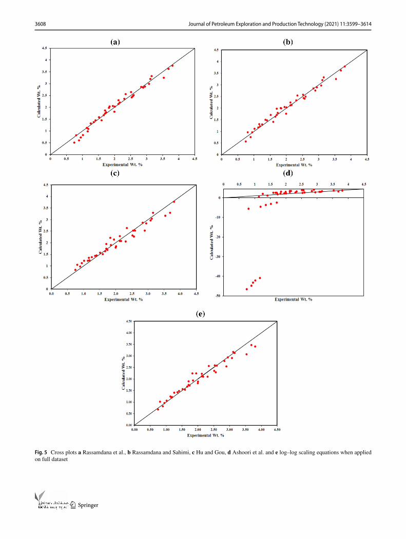
Figures 4, 5, and 6 show the cross plots between experi-mental (actual) and predicted values obtained using non-scaling models, scaling models (applied on the whole dataset), and scaling equations (when applied on partial datasets), respectively. Referring to Fig. 4, comparing the performance of non-scaling models, the PC-Saft model performed best as it is evident from the accumulation of more points on or near to the 45-degree line as compared to other models. Comparing Figs. 5 and 6, it can be depicted

Table 1 Values of tuned adjustable parameters, scaling coefficient & coefficient of determination of different scaling equations for full and par-tial datasets

Full dataset Z C1 C2 n A1 A2 A3 A4 R2

Rassamdana’s model 0.338 – – – 0.333 65.391 − 18.958 1.809 0.998Rassamdana & Sahimi model – 0.5 1.28 – 12.49 − 68.107 250.84 − 4.361 0.997Hu & Gou 0.25 0.5 − 0.4 – 4.619 − 30.819 76.705 1.905 0.986Ashoori’s model 0.25 – – 0.25 8.877 51.139 167.25 − 69.111 0.995Log–log model 0.25 – – 0.25 − 0.003 − 0.202 2.293 2.024 0.999

Partial dataset ( R ≤ 5) Z C1 C2 n A1 A2 A3 A4 R2

Rassamdana’s model 0.338 – – – 7.591 57.418 − 18.012 2.166 0.994Rassamdana & Sahimi model – 0.5 1.28 – − 2147 1123.3 76.119 1.611 0.988Hu & Gou 0.25 0.5 − 0.4 – 170.36 − 85.245 87.481 0.421 0.986Ashoori’s model 0.25 – – 0.25 126.07 − 6.396 15.747 − 1.696 0.997Log–log model 0.25 – – 0.25 − 0.653 − 0.732 2.350 2.074 0.998

Partial dataset (R > 5) Z C1 C2 n A1 A2 A3 A4 R2

Rassamdana’s model 0.338 – – – 0.370 64.607 − 14.148 − 6.127 0.997Rassamdana & Sahimi model – 0.5 1.28 – 5.074 35.287 209.62 8.364 0.991Hu & Gou 0.25 0.5 − 0.4 – 4.566 − 30.986 78.834 − 1.192 0.947Ashoori’s model 0.25 – – 0.25 33.554 − 294.23 1554.5 − 1497.1 0.994Log–log model 0.25 – – 0.25 2.418 − 4.067 4.038 1.828 0.997


1 3

Fig. 1 X and Y curves a Rassamdana et al., b Rassamdana and Sahimi, c Hu and Gou, d Ashoori et al., and e log–log scaling equations when applied of full dataset


1 3

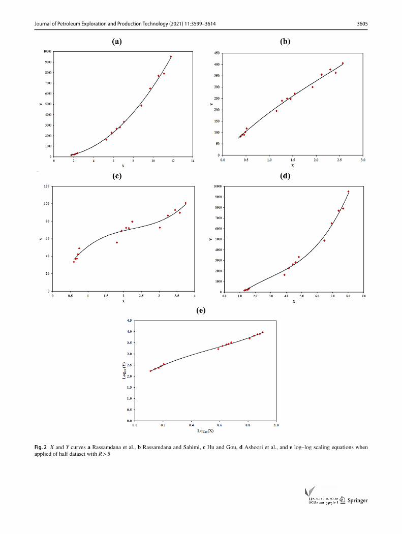
Fig. 2 X and Y curves a Rassamdana et al., b Rassamdana and Sahimi, c Hu and Gou, d Ashoori et al., and e log–log scaling equations when applied of half dataset with R > 5


1 3

Fig. 3 X and Y curves a Rassamdana et al., b Rassamdana and Sahimi, c Hu and Gou, d Ashoori et al., and e log–log scaling equations when applied of half dataset with R ≤ 5


1 3

that each scaling equation performance is improved when applied on partial datasets as the spreading of predicted results is reduced across slant lines. The highest improve-ment is observed for the Ashoori et al. scaling equation and it predicted results with quite good accuracy. Though looking at Fig. 6, it is difficult to compare the accuracies of models; however, when considered Table 2 and Fig. 6 collectively, one could confirm that Rassamdana et al. and

Rassamdana and Sahimi scaling equation performed slightly better due to the comparatively more number of points on or near to the slant line while Ashoori et al. scaling equa-tion performed relatively least due to the more spreading of predicted data across 45-degree line.

Figure 7, 8, and 9 show the relative error plot for non-scaling models, scaling equations (applied on the whole dataset), and scaling equations (applied on partial datasets),

Table 2 Mean absolute error (MAE) of scaling equations and non-scaling models (Behbahani et al. 2011)

Dataset Rassamdana et al Rassamdana & Sahimi

Hu & Gou Ashoori et al Log–log PC-Saft Solid model Flory–Huggins

Full 0.107 0.105 0.147 6.660 0.130 0.116 0.379 0.238Partial (both

R > 5 & R ≤ 50.077 0.085 0.103 0.143 0.103 – – –

Fig. 4 Cross plots a PC-Saft b Solid model c Flory–Huggins on full dataset (Behbahani et al. 2011)


1 3

Fig. 5 Cross plots a Rassamdana et al., b Rassamdana and Sahimi, c Hu and Gou, d Ashoori et al. and e log–log scaling equations when applied on full dataset


1 3

Fig. 6 Cross plots a Rassamdana et al., b Rassamdana and Sahimi, c Hu and Gou, d Ashoori et al., and e Log–log scaling equations when applied on partial datasets


1 3

respectively. Looking at Fig. 7, all non-scaling models yield under-predicted asphaltenes wt. %; however, PC-Saft com-paratively found more accurate results due to less range of error. Comparing Figs. 8 and 9, it is observed that either the range of error is reduced or the accumulation of data point is increased near or onto the horizontal line in the case of using partial datasets which indicates that the performance of scaling equations is enhanced when applied on partial datasets as compared to the whole dataset.

Table 3 shows the values of Critical Dilution Ratio (Rc) predicted by different scaling equations when applied to the whole dataset. Rassamdana et al. and Hu and Guo scal-ing equation are unable to predict onset points for differ-ent precipitants (n-alkanes) and therefore produce negative results. The main cause of this observation seems to be the curve obtained between X and Y for these models. It can be observed in Fig. 1a and c that the curves of these two

scaling equations are going to meet the x-axis at the negative side when Y = 0. On the other hand, Ashoori et al. and the log–log scaling equations overpredict the results, whereas Rassamadana and Sahimi scaling equations underpredict the results. The nearest results are predicted by a log–log scaling equation with significant error.

Table 4 illustrates the predicted values of critical dilution ratio (Rc) by different scaling equations when applied on the partial dataset (R ≤ 5). Rassamdana et al., Rassamadana, and Sahimi, and Hu and Guo’s scaling equations could not find the onset point since their XY curve goes to intersect the negative x-axis at Y = 0 as shown in Fig. 3a, b, and c. Log–log scaling equation produces approximately the same onset points for all precipitants as produced while using the whole dataset. Ashoori et al. scaling equation predicted excellent results.

Fig. 7 Relative Error plots a PC-Saft b solid model c Flory–Huggins on full datasets (Behbahani et al. 2011)


1 3

Fig. 8 Relative error plot a Rassamdana et al., b Rassamdana and Sahimi, c Hu and Gou, d Ashoori et al., and e Log–log scaling equations when applied on full dataset


1 3

Fig. 9 Relative Error plot a Rassamdana et al., b Rassamdana and Sahimi, c Hu and Gou, d Ashoori et al., and e Log–log scaling equations when applied on partial datasets‏


1 3

Table 5 presents the onset results predicted and perfor-mance comparison between all non-scaling models and the best scaling equation, i.e., Ashoori et al. scaling equation in this case. It is observed that the Ashoori et al. scaling equation yields more accurate results as compared to other non-scaling models.

Conclusion

The following conclusions can be drawn from this study:

1. Scaling equations performance, in terms of predicting asphaltene weight percentage, is enhanced when applied on datasets formed by splitting the full dataset with respect to dilution ratio.

2. Scaling equations are capable of predicting asphaltene weight percentage with good accuracy when applied on full dataset as well as by using partial datasets except for Ashoori et al. scaling equation when applied on the full dataset.

3. Scaling equations are not good predictors of critical dilu-tion ratio (Rc) except for Ashoori et al. scaling equation which produces excellent results when utilized partial dataset (R ≤ 5) for prediction.

4. Comparing the performance of scaling equations with non-scaling models for predicting the asphaltene weight percentage, all scaling equations yield almost the same or better results as compared to the best case of non-scaling models which is the PC-Saft model.

5. Comparing the performance of scaling equations with non-scaling models for predicting the critical dilution ratio, the non-scaling models perform better. In most cases, scaling equations are unable to predict Rc or pro-duce results of considerable error. Non-scaling models produce less accurate results as compared to Ashoori et scaling equation when utilized partial dataset (R ≤ 5) for prediction.

6. Summarizing the study, it is suggested that the asphaltene modeling in dead crude oils, both for predicting onset point and asphaltene weight percent, could be achieved by Ashoori et al. scaling equation with good accuracy when applied on splitting the full datasets concerning dilution

Table 3 Values of Rc obtained for different precipitants using the full dataset

Precipitant Rassamdana et al Rassamdana & Sahimi

Hu & Gou Ashoori et al Log–log

n − C5 − 573.02 0.317 − 0.328 2.300 0.935n − C6 − 599.05 0.346 − 0.343 2.405 0.977n − C7 − 622.07 0.373 − 0.356 2.498 1.015n − C9 − 661.67 0.423 − 0.379 2.657 1.079n − C12 − 710.31 0.487 − 0.407 2.851 1.159

Table 4 Values of Rc obtained for different precipitants using partial dataset R ≤ 5

Precipitant Rassamdana et al Rassamdana & Sahimi Hu & Gou Ashoori et al Log–log

n − C5 − 22.926 − 3.264E + 13 − 0.064 0.643 0.931n − C6 − 23.967 − 3.567E + 13 − 0.066 0.672 0.973n − C7 − 24.888 − 3.847E + 13 − 0.069 0.698 1.010n − C9 − 26.473 − 4.352E + 13 − 0.073 0.743 1.075n − C12 − 28.419 − 5.016E + 13 − 0.793 0.797 1.154

Table 5 Rc values obtained from different precipitants and mean absolute error (MAE) of experimental (Behbahani et al. 2011), non-scaling models (Behbahani et al. 2011), and Ashoori et al. scaling equation

Bold values indicate MAE results

Precipitant Experiment onset

PC-Saft Flory–Huggins Solid model Ashoori et al

n − C5 0.65 0.69 0.72 0.74 0.644n − C6 0.7 0.74 0.79 0.83 0.673n − C7 0.72 0.78 0.84 0.84 0.699n − C9 0.78 0.82 0.86 0.87 0.743n − C12 0.84 0.89 0.92 0.94 0.798MAE – 0.046 0.088 0.106 0.027


1 3

ratio. On splitted datasets, Ashoori et al. scaling equation found asphaltene weight percentages with mean absolute error of 0.143 which is slightly greater than other scaling model but still very less. The biggest advantage of using this equation is its excellent ability of predicting onset point when other scaling equations are completely failed. Ashoori et al. scaling equation yields only 0.027 of MAE while estimating onset point (Rc) even better than non-scaling models. Moreover, this scaling equation does not require crude oil properties and offer fewer computation complexities as compared to non-scaling models.

Funding There is no funding agency involved.

Declarations

Conflict of interest The authors have no conflicts of interest to declare that are relevant to the content of this article.

Open Access This article is licensed under a Creative Commons Attri-bution 4.0 International License, which permits use, sharing, adapta-tion, distribution and reproduction in any medium or format, as long as you give appropriate credit to the original author(s) and the source, provide a link to the Creative Commons licence, and indicate if changes were made. The images or other third party material in this article are included in the article’s Creative Commons licence, unless indicated otherwise in a credit line to the material. If material is not included in the article’s Creative Commons licence and your intended use is not permitted by statutory regulation or exceeds the permitted use, you will need to obtain permission directly from the copyright holder. To view a copy of this licence, visit http:// creat iveco mmons. org/ licen ses/ by/4. 0/.

References

Agrawala M, Yarranton HW (2001) An asphaltene association model analogous to linear polymerization. Ind Eng Chem Res 40:4664–4672

Alhosani A, Daraboina N (2020) Unified model to predict asphaltene deposition in production pipelines. Energy Fuels 34:1720–1727

Ali SI, Lalji SM, Haneef J, Ahsan U, Tariq SM, Tirmizi ST, Shamim R (2021) Critical analysis of different techniques used to screen asphaltene stability in crude oils. Fuel 299:120874

Alimohammadi S, Amin JS, Nikooee E (2017) Estimation of asphal-tene precipitation in light, medium and heavy oils: experimen-tal study and neural network modeling. Neural Comput & Appl 28:679–694

Alimohammadi S, Amin JS, Nikkhah S, Soroush M, Zendehboudi S (2020) Development of a new scaling model for asphaltene precipitation in light, medium, and heavy crude oils. J Mol Liq 312:112974

Ashoori S, Jamialahmadi M, Müller-Steinhagen H, Ahmadi K (2003) A New Scaling Equation for Modeling of Asphaltene Precipita-tion. In: 27th Annual SPE International Technical Conference and Exhibition, Society of Petroleum Engineers

Ashoori S, Sharifi M, Masoumi M, Salehi MM (2017) The relation-ship between SARA fractions and crude oil stability. Egypt J Pet 2017(26):209–213

Bahman J, Sharifi K, Nasiri M, Asl MH (2018) Development of a Log-Log scaling law approach for prediction of asphaltene

precipitation from crude oil by n-alkane titration. J Pet Sci Eng 160:393–400

Behbahani TJ, Ghotbi C, Taghikhani V, Shahrabadi A (2011) Experi-mental investigation and thermodynamic modeling of asphaltene precipitation. Sci Iran c 18:1384–1390

Firoozinia H, Abad KFH, Varamesh A (2016) A comprehensive experi-mental evaluation of asphaltene dispersants for injection under reservoir conditions. Pet Sci 13:280–291

Gharbi K, Benyounes K, Khodja M (2017) Removal and prevention of asphaltene deposition during oil production: a literature review. J Petrol Sci Eng 58:351–360

Hu Y-F, Guo T-M (2000) Effect of temperature and molecular weight of n-alkane precipitants on asphaltene precipitation. Fluid Phase Equilib 192:13–25

Hu Y-F, Chen G-J, Yang J-T, Guo T-M (2000) A study on the applica-tion of scaling equation for asphaltene precipitation. Fluid Phase Equilib 171:181–195

Leontaritis K, Mansoori GA (1987) Asphaltene flocculation during oil production and processing: a thermodynamic collodial model. In: SPE International Symposium on Oilfield Chemistry, Society of Petroleum Engineers, San Antonio, US

Melendez-Alvarez AA, Garcia-Bermudes M, Tavakkoli M, Doherty RH, Meng S, Abdallah DS, Vargas FM (2016) On the evaluation of the performance of asphaltene dispersants. Fuel 179:210–220

Moghadasi R (2019) A critical review on asphaltenes scaling equations. Pet Sci Technol 37:2142–2145

Mohammadi AH, Eslamimanesh A, Richon D (2012) Monodisperse thermodynamic model based on chemical + flory−hüggins poly-mer solution theories for predicting asphaltene precipitation. Ind Eng Chem Res 51:4041–4055

Mohammed I, Mahmoud M, Al Shehri D, El-Husseiny A, Alade O (2021) Asphaltene precipitation and deposition: a critical review. J Pet Sci Eng 197:107956

Panuganti SR, Vargas FM, Gonzalez DL, Kurup AS, Chapman WG (2012) PC-SAFT characterization of crude oils and modeling of asphaltene phase behavior. Fuel 93:658–669

Rassamdana H, Sahimi M (1996) Asphalt flocculation and deposi-tion: II formation and growth of fractal aggregates. AIChE J 42:3318–3332

Rassamdana H, Dabir B, Nematy M, Farhani M, Sahimi M (1996) Asphalt flocculation and deposition: I. The onset of precipitation. AIChE J 42:10–22

Subramanian S, Simon S, Sjöblom J (2016) Asphaltene precipitation models: a review. J Dispers Sci Technol 37:1027–1049

Victorov AI, Firoozabadi A (1996) Thermodynamic micellization model of asphaltene precipitation from petroleum fluids. AIChE J 42:1753–1764

Zendehboudi S, Ahmadi MA, Mohammadzadeh O, Bahadori A, Chatzis I (2013) Thermodynamic investigation of asphaltene pre-cipitation during primary oil production: laboratory and smart technique. Ind Eng Chem Res 52:6009–6031

Zendehboudi S, Shafiei A, Bahadori A, James LA, Elkamel A, Lohi A (2014) Asphaltene precipitation and deposition in oil reser-voirs—Technical aspects, experimental and hybrid neural network predictive tools. Chem Eng Res Des 92:857–875

Zhang X, Pedrosa N, Moorwood T (2012) Modeling asphaltene phase behavior: comparison of methods for flow assurance studies. Energy Fuels 26:2611–2620

Zheng F, Shi Q, Vallverdu G, Giusti P, Bouyssière B (2020) Frac-tionation and Characterization of Petroleum Asphaltene: Focus on Metalopetroleomics, Processes, MDPI

Publisher’s note Springer Nature remains neutral with regard to jurisdictional claims in published maps and institutional affiliations.

http://creativecommons.org/licenses/by/4.0/

asphaltene precipitation modeling in dead crude oils using

Documents