Chapter 03 Assemblers

Nov 2007

MU-MIT

Outline• This chapter is organized into four/five

sections listed below.• 3 Assemblers• 3.1 General design procedure• 3.2 Design of assembler

• Statement of problem

• Data structure

• Format of databases

• Algorithms

• Look for modularity

• 3.3 Table processing • Sorting

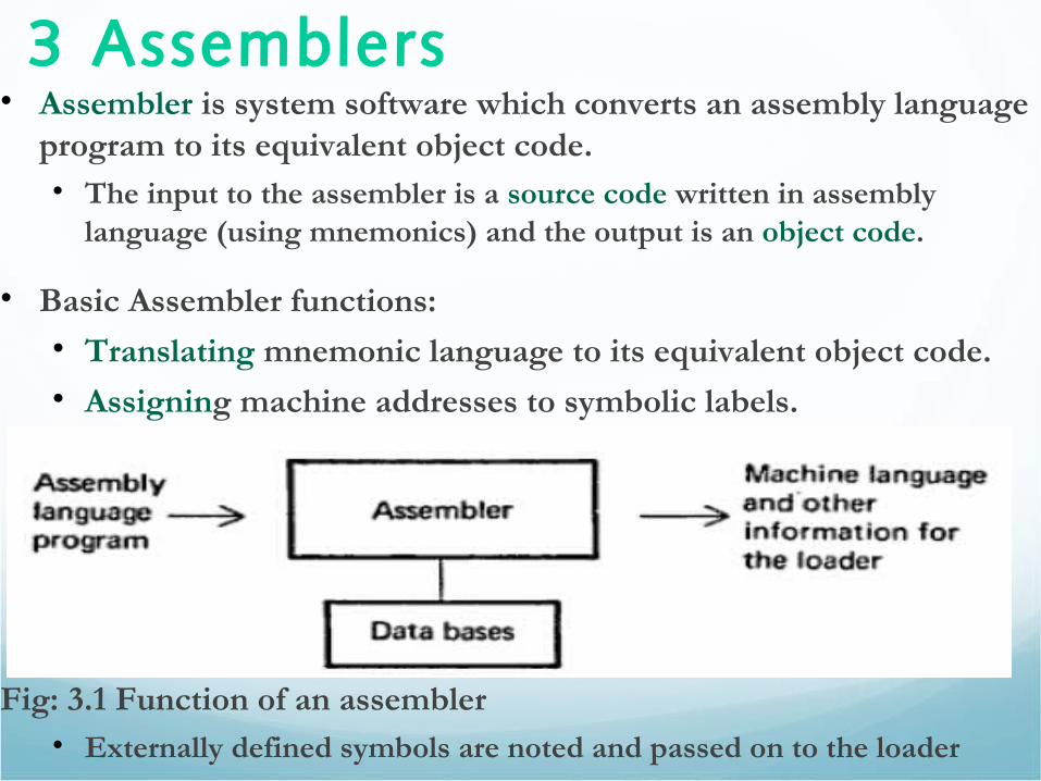
3 Assemblers• Assembler is system software which converts an assembly language

program to its equivalent object code. • The input to the assembler is a source code written in assembly

language (using mnemonics) and the output is an object code.

• Basic Assembler functions:• Translating mnemonic language to its equivalent object code.• Assigning machine addresses to symbolic labels.

Fig: 3.1 Function of an assembler • Externally defined symbols are noted and passed on to the loader

3.1 General Design Procedure• In our design of an assembler, we are interested in producing

machine language from a given assembly language.

• Let’s start with the general problem of designing a software. We usually follow the following steps to design a software.1. Specify the problem: specify all the requirements2. Specify the data structure: (use set of tables) List out tables

with fields (eg. Symbol table, opcode table, size of instruction )3. Define format of data structure: formats of database to be

used 4. Specify algorithm:

• Scan the program for labels-> first pass algorithm

• Use for translation-> second pass algorithm

1. Look for modularity – divide program into smaller modules2. Repeat 1 ~ 5 on modules

These general software design procedure will be employed in our assembler design in this chapter……

3.2 Design of an Assembler

• In this section we will discuss the fundamental Assembler design procedures using relevant examples and justifications. The topics that will be discussed in this section are:• Statement of problem

• Data structure

• Format of databases

• Algorithms

• Look for modularity

• Simple example Assembly Language programs will be used to show how assemblers work.

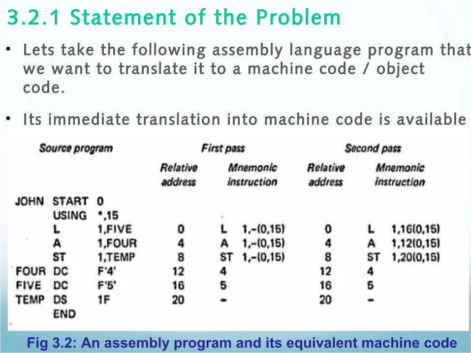
3.2.1 Statement of the Problem• Lets take the following assembly language program that

we want to translate it to a machine code / object code.

• Its immediate translation into machine code is avai lable on the right side.

Fig 3.2: An assembly program and its equivalent machine code

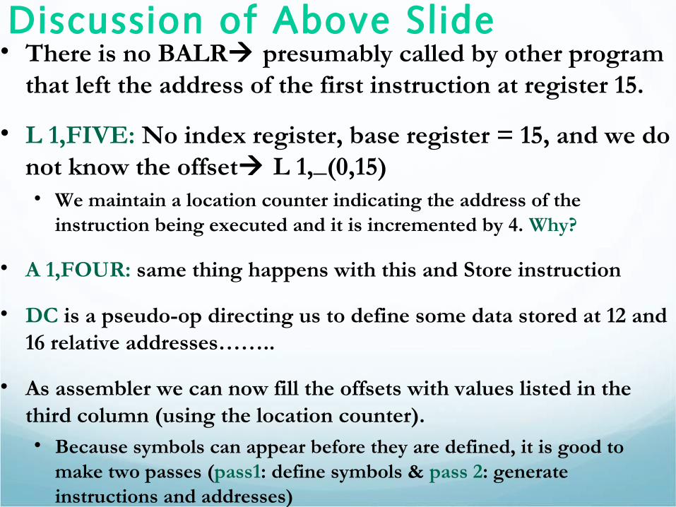
Discussion of Above Sl ide• There is no BALR presumably called by other program

that left the address of the first instruction at register 15.

• L 1,FIVE: No index register, base register = 15, and we do not know the offset L 1,_(0,15)• We maintain a location counter indicating the address of the

instruction being executed and it is incremented by 4. Why?

• A 1,FOUR: same thing happens with this and Store instruction

• DC is a pseudo-op directing us to define some data stored at 12 and 16 relative addresses……..

• As assembler we can now fill the offsets with values listed in the third column (using the location counter).• Because symbols can appear before they are defined, it is good to

make two passes (pass1: define symbols & pass 2: generate instructions and addresses)

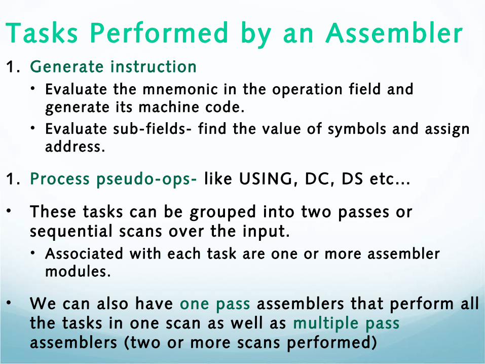
Tasks Performed by an Assembler1. Generate instruction

• Evaluate the mnemonic in the operation field and generate its machine code.

• Evaluate sub-fields- find the value of symbols and assign address.

1. Process pseudo-ops- l ike USING, DC, DS etc…

• These tasks can be grouped into two passes or sequential scans over the input.• Associated with each task are one or more assembler

modules.

• We can also have one pass assemblers that perform all the tasks in one scan as well as multiple pass assemblers (two or more scans performed)

Two Pass Assemblers

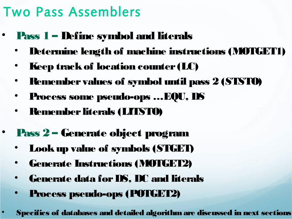
• Pass 1 – Define symbol and literals• Determine length of machine instructions (MOTGET1)• Keep track of location counter (LC)• Remember values of symbol until pass 2 (STSTO)• Process some pseudo-ops …EQU, DS• Remember literals (LITSTO)

• Pass 2 – Generate object program• Look up value of symbols (STGET)• Generate Instructions (MOTGET2)• Generate data for DS, DC and literals• Process pseudo-ops (POTGET2)

• Specifics of databases and detailed algorithm are discussed in next sections

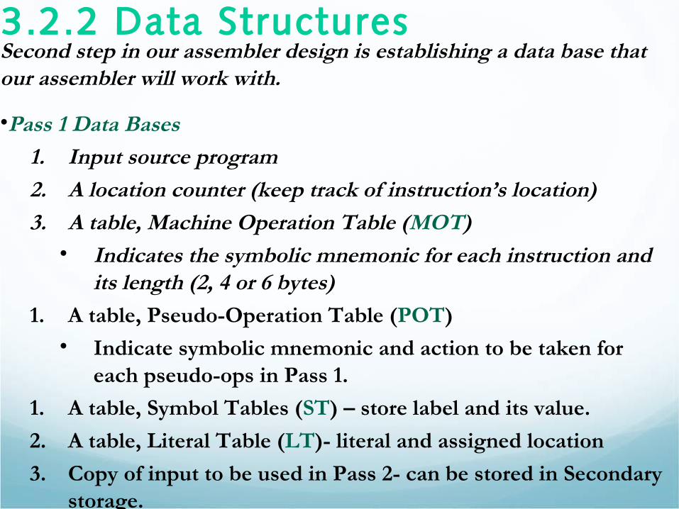
3.2.2 Data StructuresSecond step in our assembler design is establishing a data base that our assembler will work with.

•Pass 1 Data Bases1. Input source program2. A location counter (keep track of instruction’s location)3. A table, Machine Operation Table (MOT)• Indicates the symbolic mnemonic for each instruction and

its length (2, 4 or 6 bytes)1. A table, Pseudo-Operation Table (POT)• Indicate symbolic mnemonic and action to be taken for

each pseudo-ops in Pass 1.

1. A table, Symbol Tables (ST) – store label and its value.

2. A table, Literal Table (LT)- literal and assigned location

3. Copy of input to be used in Pass 2- can be stored in Secondary storage.

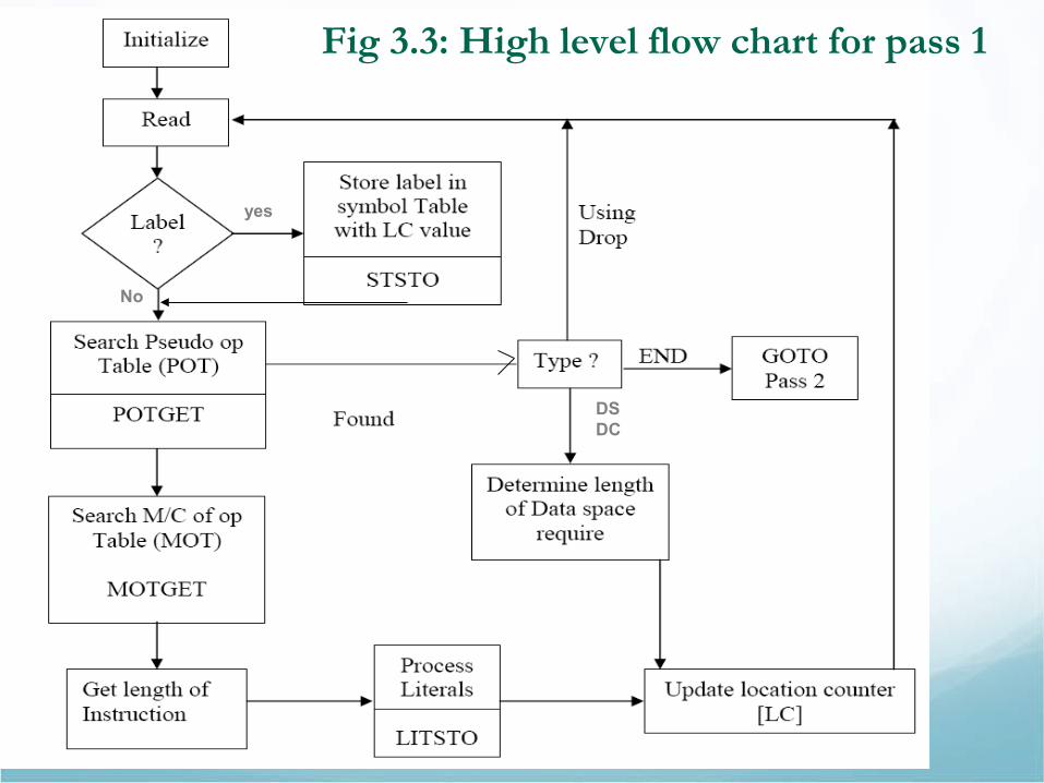
Fig 3.3: High level flow chart for pass 1

yes

No

DSDC

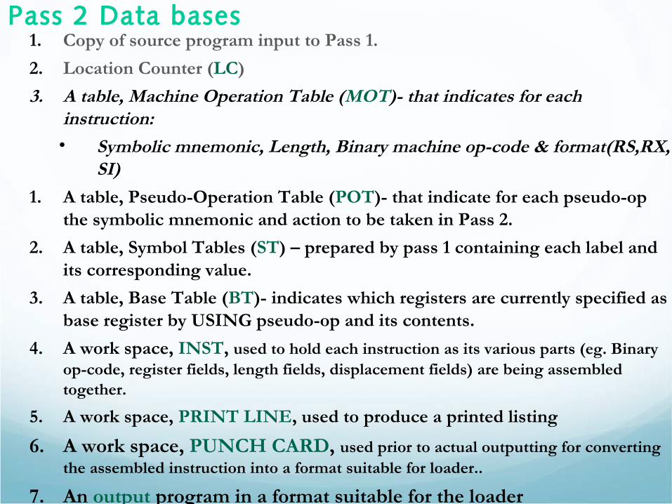
Pass 2 Data bases1. Copy of source program input to Pass 1.

2. Location Counter (LC)

3. A table, Machine Operation Table (MOT)- that indicates for each instruction:• Symbolic mnemonic, Length, Binary machine op-code & format(RS,RX,

SI)

1. A table, Pseudo-Operation Table (POT)- that indicate for each pseudo-op the symbolic mnemonic and action to be taken in Pass 2.

2. A table, Symbol Tables (ST) – prepared by pass 1 containing each label and its corresponding value.

3. A table, Base Table (BT)- indicates which registers are currently specified as base register by USING pseudo-op and its contents.

4. A work space, INST, used to hold each instruction as its various parts (eg. Binary op-code, register fields, length fields, displacement fields) are being assembled together.

5. A work space, PRINT LINE, used to produce a printed listing

6. A work space, PUNCH CARD, used prior to actual outputting for converting the assembled instruction into a format suitable for loader..

7. An output program in a format suitable for the loader

Fig 3.4: Pass 2 OverviewEvaluate Fields and Generic Code

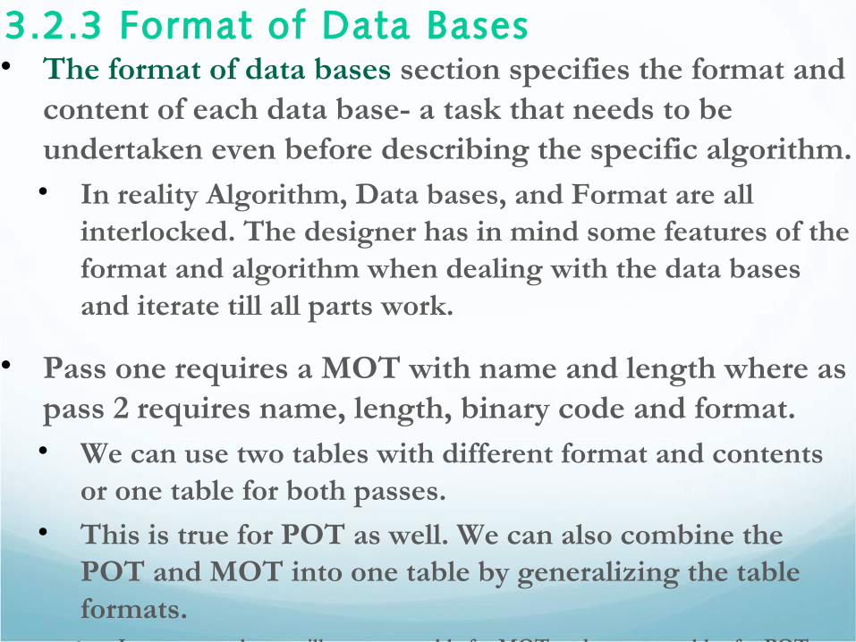
3.2.3 Format of Data Bases• The format of data bases section specifies the format and

content of each data base- a task that needs to be undertaken even before describing the specific algorithm.• In reality Algorithm, Data bases, and Format are all

interlocked. The designer has in mind some features of the format and algorithm when dealing with the data bases and iterate till all parts work.

• Pass one requires a MOT with name and length where as pass 2 requires name, length, binary code and format.• We can use two tables with different format and contents

or one table for both passes.• This is true for POT as well. We can also combine the

POT and MOT into one table by generalizing the table formats.• In our example we will use same table for MOT and separate tables for POT.

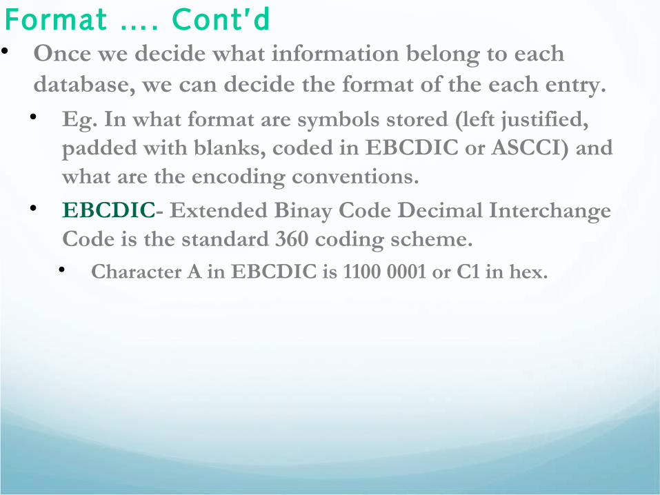
Format …. Cont’d• Once we decide what information belong to each

database, we can decide the format of the each entry.• Eg. In what format are symbols stored (left justified,

padded with blanks, coded in EBCDIC or ASCCI) and what are the encoding conventions.

• EBCDIC- Extended Binay Code Decimal Interchange Code is the standard 360 coding scheme.• Character A in EBCDIC is 1100 0001 or C1 in hex.

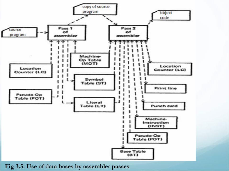
Fig 3.5: Use of data bases by assembler passes

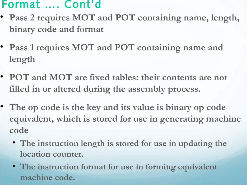
Format …. Cont’d• Pass 2 requires MOT and POT containing name, length,

binary code and format

• Pass 1 requires MOT and POT containing name and length

• POT and MOT are fixed tables: their contents are not filled in or altered during the assembly process.

• The op code is the key and its value is binary op code equivalent, which is stored for use in generating machine code• The instruction length is stored for use in updating the

location counter. • The instruction format for use in forming equivalent

machine code.

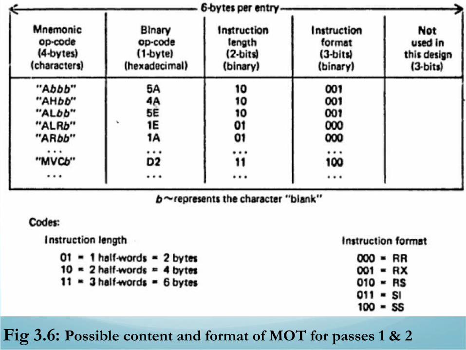
Fig 3.6: Possible content and format of MOT for passes 1 & 2

Fig 3.7: Possible content and format of POT for pass 1 (similar for pass 2)

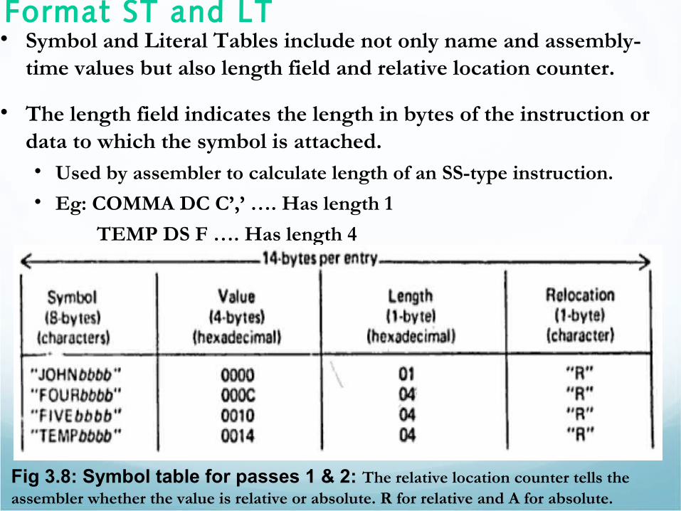
Format ST and LT• Symbol and Literal Tables include not only name and assembly-

time values but also length field and relative location counter.

• The length field indicates the length in bytes of the instruction or data to which the symbol is attached.• Used by assembler to calculate length of an SS-type instruction.

• Eg: COMMA DC C’,’ …. Has length 1

TEMP DS F …. Has length 4

Fig 3.8: Symbol table for passes 1 & 2: The relative location counter tells the assembler whether the value is relative or absolute. R for relative and A for absolute.

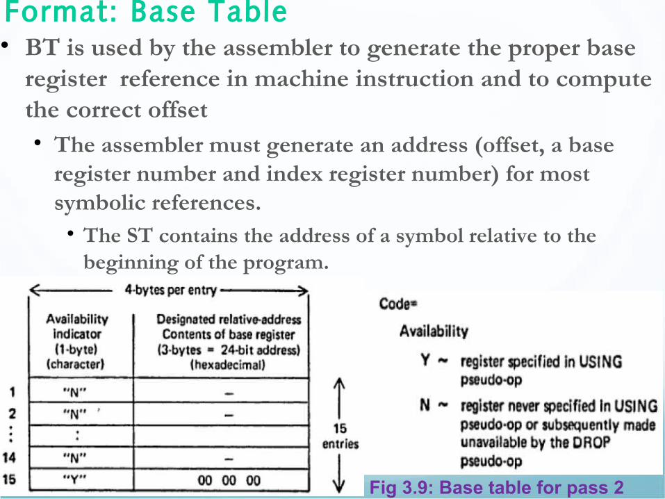
Format: Base Table• BT is used by the assembler to generate the proper base

register reference in machine instruction and to compute the correct offset• The assembler must generate an address (offset, a base

register number and index register number) for most symbolic references. • The ST contains the address of a symbol relative to the

beginning of the program.

Fig 3.9: Base table for pass 2

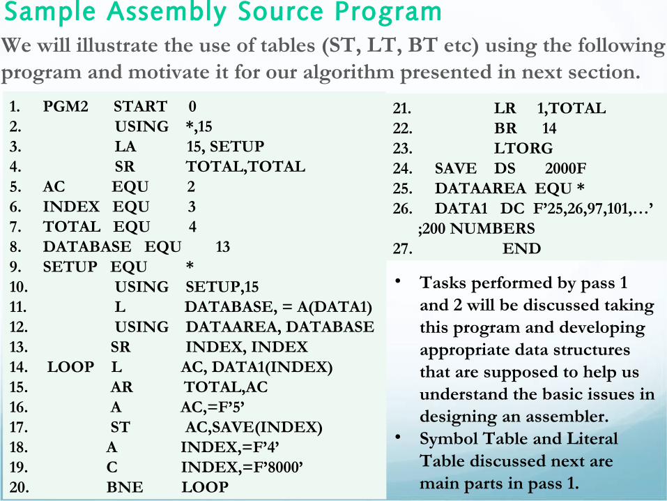
Sample Assembly Source ProgramWe will illustrate the use of tables (ST, LT, BT etc) using the following program and motivate it for our algorithm presented in next section.

1. PGM2 START 02. USING *,153. LA 15, SETUP4. SR TOTAL,TOTAL5. AC EQU 26. INDEX EQU 37. TOTAL EQU 48. DATABASE EQU 139. SETUP EQU *10. USING SETUP,15 11. L DATABASE, = A(DATA1)12. USING DATAAREA, DATABASE13. SR INDEX, INDEX14. LOOP L AC, DATA1(INDEX)15. AR TOTAL,AC16. A AC,=F’5’17. ST AC,SAVE(INDEX)18. A INDEX,=F’4’19. C INDEX,=F’8000’20. BNE LOOP

21. LR 1,TOTAL22. BR 1423. LTORG24. SAVE DS 2000F 25. DATAAREA EQU *26. DATA1 DC F’25,26,97,101,…’

;200 NUMBERS27. END

• Tasks performed by pass 1 and 2 will be discussed taking this program and developing appropriate data structures that are supposed to help us understand the basic issues in designing an assembler.

• Symbol Table and Literal Table discussed next are main parts in pass 1.

Pass 1: Define Symbols and Literals

Symbol Table

Literal Table

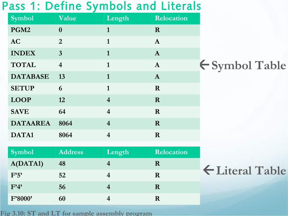
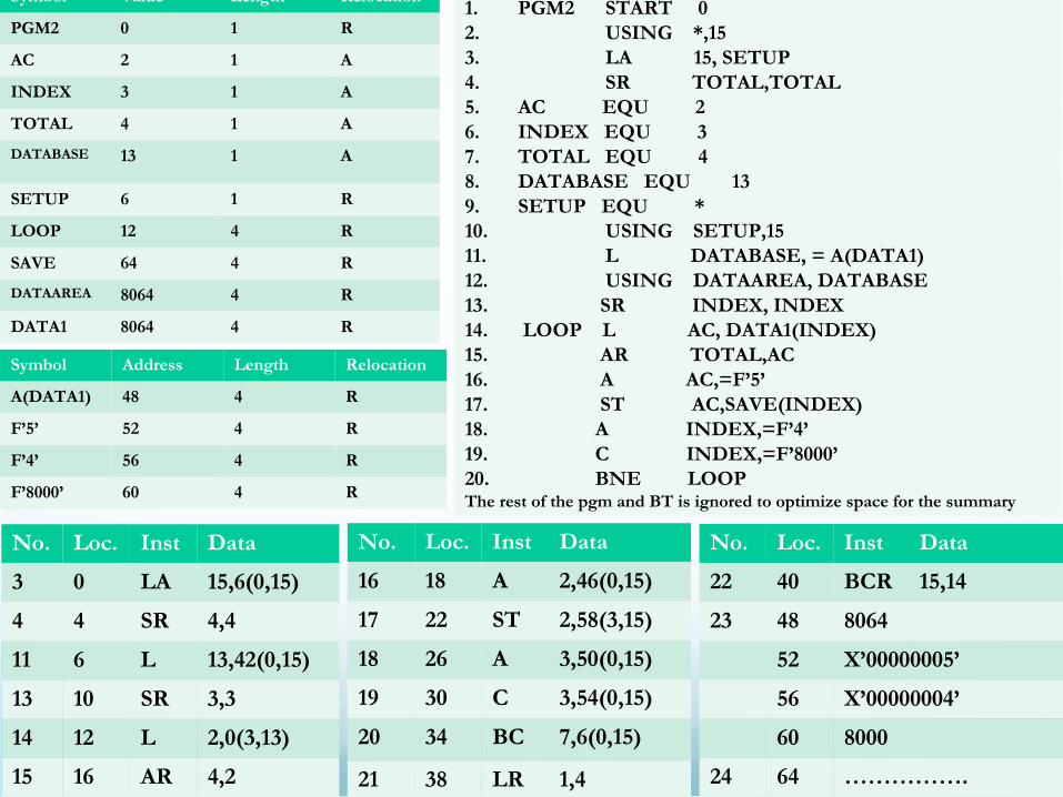
Fig 3.10: ST and LT for sample assembly program

Symbol Value Length Relocation

PGM2 0 1 R

AC 2 1 A

INDEX 3 1 A

TOTAL 4 1 A

DATABASE 13 1 A

SETUP 6 1 R

LOOP 12 4 R

SAVE 64 4 R

DATAAREA 8064 4 R

DATA1 8064 4 R

Symbol Address Length Relocation

A(DATA1) 48 4 R

F’5’ 52 4 R

F’4’ 56 4 R

F’8000’ 60 4 R

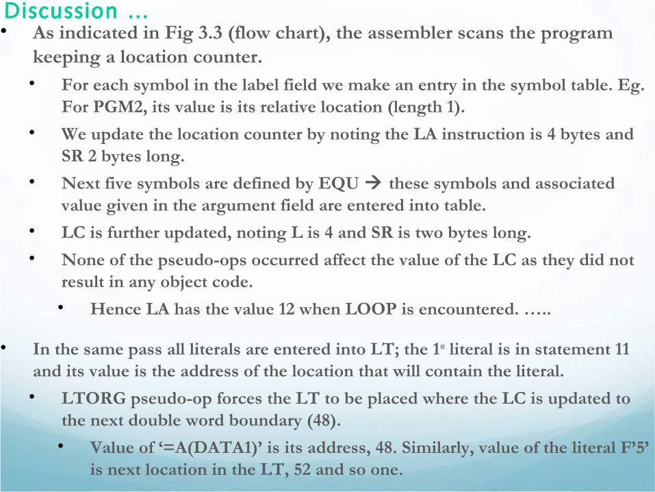
Discussion …• As indicated in Fig 3.3 (flow chart), the assembler scans the program

keeping a location counter.• For each symbol in the label field we make an entry in the symbol table. Eg.

For PGM2, its value is its relative location (length 1).

• We update the location counter by noting the LA instruction is 4 bytes and SR 2 bytes long.

• Next five symbols are defined by EQU these symbols and associated value given in the argument field are entered into table.

• LC is further updated, noting L is 4 and SR is two bytes long.

• None of the pseudo-ops occurred affect the value of the LC as they did not result in any object code.

• Hence LA has the value 12 when LOOP is encountered. …..

• In the same pass all literals are entered into LT; the 1st literal is in statement 11 and its value is the address of the location that will contain the literal.

• LTORG pseudo-op forces the LT to be placed where the LC is updated to the next double word boundary (48).

• Value of ‘=A(DATA1)’ is its address, 48. Similarly, value of the literal F’5’ is next location in the LT, 52 and so one.

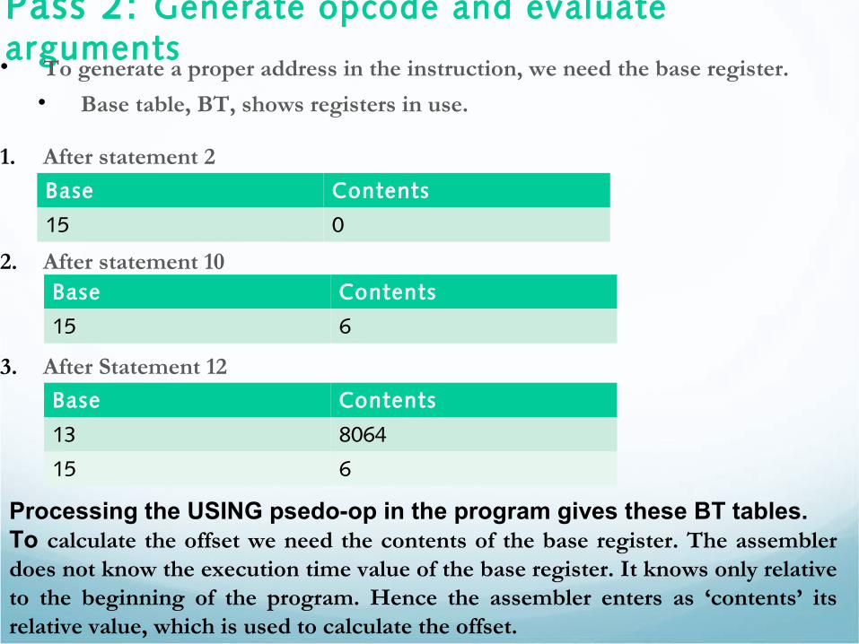
Pass 2: Generate opcode and evaluate arguments• To generate a proper address in the instruction, we need the base register.

• Base table, BT, shows registers in use.

1. After statement 2

2. After statement 10

3. After Statement 12

Base Contents

15 0

Base Contents

15 6

Base Contents

13 8064

15 6

Processing the USING psedo-op in the program gives these BT tables.To calculate the offset we need the contents of the base register. The assembler does not know the execution time value of the base register. It knows only relative to the beginning of the program. Hence the assembler enters as ‘contents’ its relative value, which is used to calculate the offset.

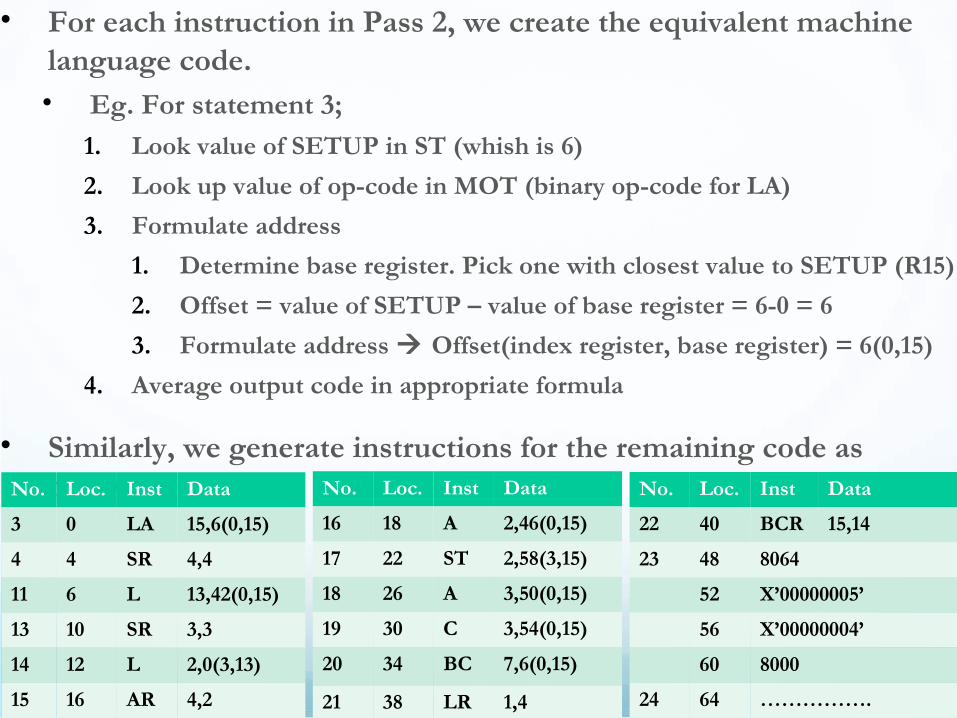
• For each instruction in Pass 2, we create the equivalent machine language code. • Eg. For statement 3;

1. Look value of SETUP in ST (whish is 6)

2. Look up value of op-code in MOT (binary op-code for LA)

3. Formulate address

1. Determine base register. Pick one with closest value to SETUP (R15)

2. Offset = value of SETUP – value of base register = 6-0 = 6

3. Formulate address Offset(index register, base register) = 6(0,15)

4. Average output code in appropriate formula

• Similarly, we generate instructions for the remaining code as below..No. Loc. Inst Data

3 0 LA 15,6(0,15)

4 4 SR 4,4

11 6 L 13,42(0,15)

13 10 SR 3,3

14 12 L 2,0(3,13)

15 16 AR 4,2

No. Loc. Inst Data

16 18 A 2,46(0,15)

17 22 ST 2,58(3,15)

18 26 A 3,50(0,15)

19 30 C 3,54(0,15)

20 34 BC 7,6(0,15)

21 38 LR 1,4

No. Loc. Inst Data

22 40 BCR 15,14

23 48 8064

52 X’00000005’

56 X’00000004’

60 8000

24 64 …………….

Symbol Value Length Relocation

PGM2 0 1 R

AC 2 1 A

INDEX 3 1 A

TOTAL 4 1 A

DATABASE 13 1 A

SETUP 6 1 R

LOOP 12 4 R

SAVE 64 4 R

DATAAREA 8064 4 R

DATA1 8064 4 R

No. Loc. Inst Data

3 0 LA 15,6(0,15)

4 4 SR 4,4

11 6 L 13,42(0,15)

13 10 SR 3,3

14 12 L 2,0(3,13)

15 16 AR 4,2

No. Loc. Inst Data

16 18 A 2,46(0,15)

17 22 ST 2,58(3,15)

18 26 A 3,50(0,15)

19 30 C 3,54(0,15)

20 34 BC 7,6(0,15)

21 38 LR 1,4

No. Loc. Inst Data

22 40 BCR 15,14

23 48 8064

52 X’00000005’

56 X’00000004’

60 8000

24 64 …………….

1. PGM2 START 02. USING *,153. LA 15, SETUP4. SR TOTAL,TOTAL5. AC EQU 26. INDEX EQU 37. TOTAL EQU 48. DATABASE EQU 139. SETUP EQU *10. USING SETUP,15 11. L DATABASE, = A(DATA1)12. USING DATAAREA, DATABASE13. SR INDEX, INDEX14. LOOP L AC, DATA1(INDEX)15. AR TOTAL,AC16. A AC,=F’5’17. ST AC,SAVE(INDEX)18. A INDEX,=F’4’19. C INDEX,=F’8000’20. BNE LOOPThe rest of the pgm and BT is ignored to optimize space for the summary

Symbol Address Length Relocation

A(DATA1) 48 4 R

F’5’ 52 4 R

F’4’ 56 4 R

F’8000’ 60 4 R

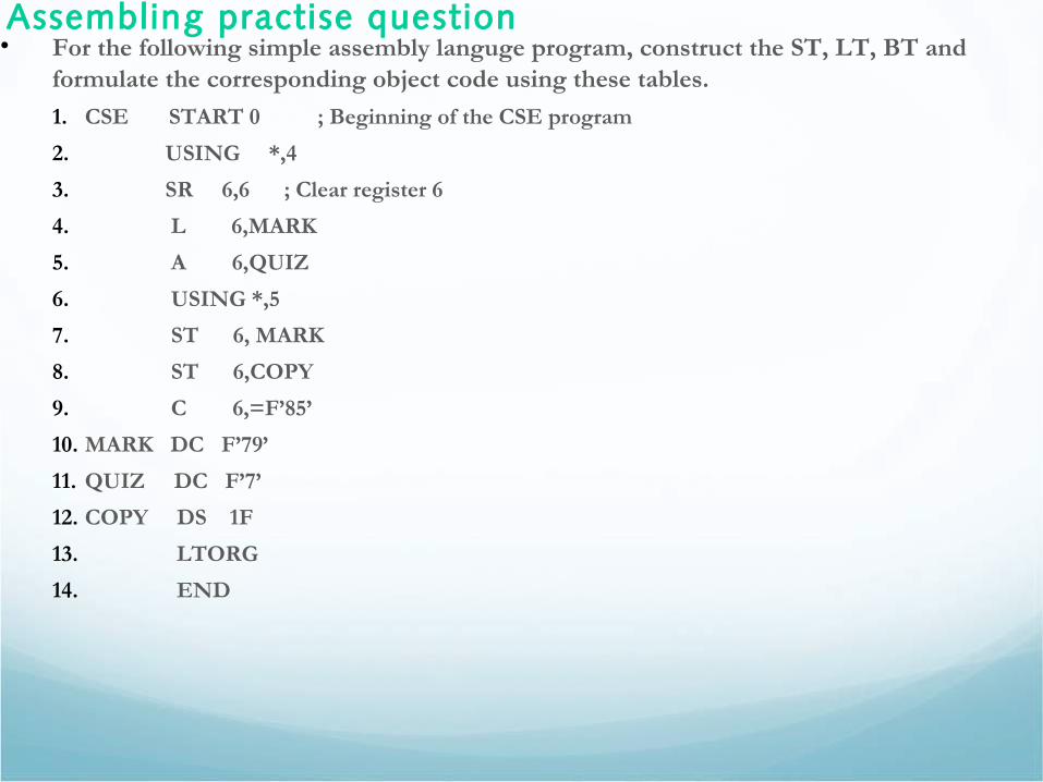
Assembling practise question• For the following simple assembly languge program, construct the ST, LT, BT and

formulate the corresponding object code using these tables.

1. CSE START 0 ; Beginning of the CSE program

2. USING *,4

3. SR 6,6 ; Clear register 6

4. L 6,MARK

5. A 6,QUIZ

6. USING *,5

7. ST 6, MARK

8. ST 6,COPY

9. C 6,=F’85’

10. MARK DC F’79’

11. QUIZ DC F’7’

12. COPY DS 1F

13. LTORG

14. END

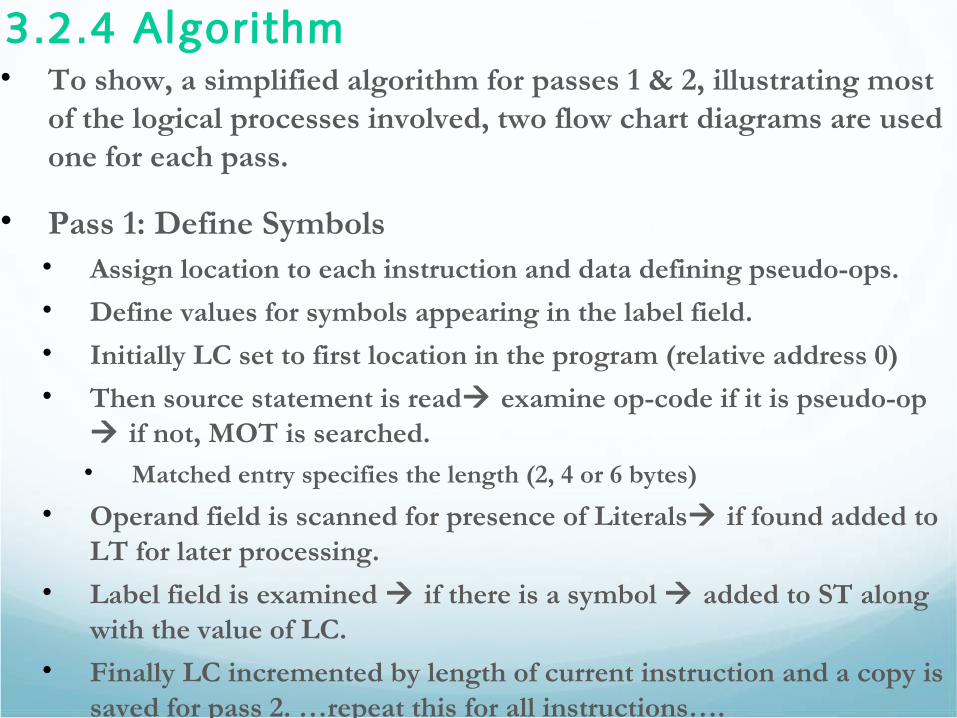
3.2.4 Algorithm• To show, a simplified algorithm for passes 1 & 2, illustrating most

of the logical processes involved, two flow chart diagrams are used one for each pass.

• Pass 1: Define Symbols• Assign location to each instruction and data defining pseudo-ops.

• Define values for symbols appearing in the label field.

• Initially LC set to first location in the program (relative address 0)

• Then source statement is read examine op-code if it is pseudo-op if not, MOT is searched. • Matched entry specifies the length (2, 4 or 6 bytes)

• Operand field is scanned for presence of Literals if found added to LT for later processing.

• Label field is examined if there is a symbol added to ST along with the value of LC.

• Finally LC incremented by length of current instruction and a copy is saved for pass 2. …repeat this for all instructions….

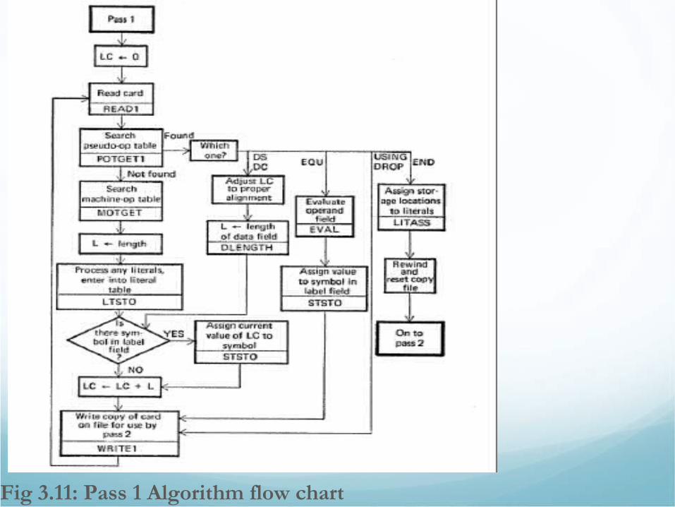
Fig 3.11: Pass 1 Algorithm flow chart

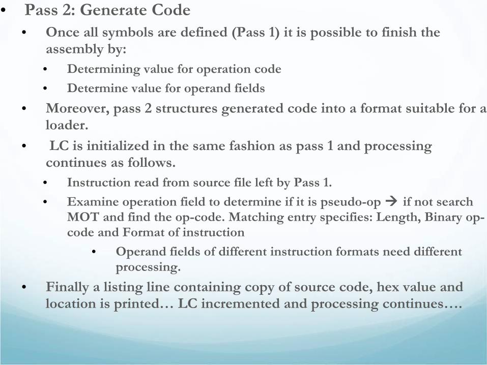
• Pass 2: Generate Code• Once all symbols are defined (Pass 1) it is possible to finish the

assembly by:• Determining value for operation code

• Determine value for operand fields

• Moreover, pass 2 structures generated code into a format suitable for a loader.

• LC is initialized in the same fashion as pass 1 and processing continues as follows.• Instruction read from source file left by Pass 1.

• Examine operation field to determine if it is pseudo-op if not search MOT and find the op-code. Matching entry specifies: Length, Binary op-code and Format of instruction

• Operand fields of different instruction formats need different processing.

• Finally a listing line containing copy of source code, hex value and location is printed… LC incremented and processing continues….

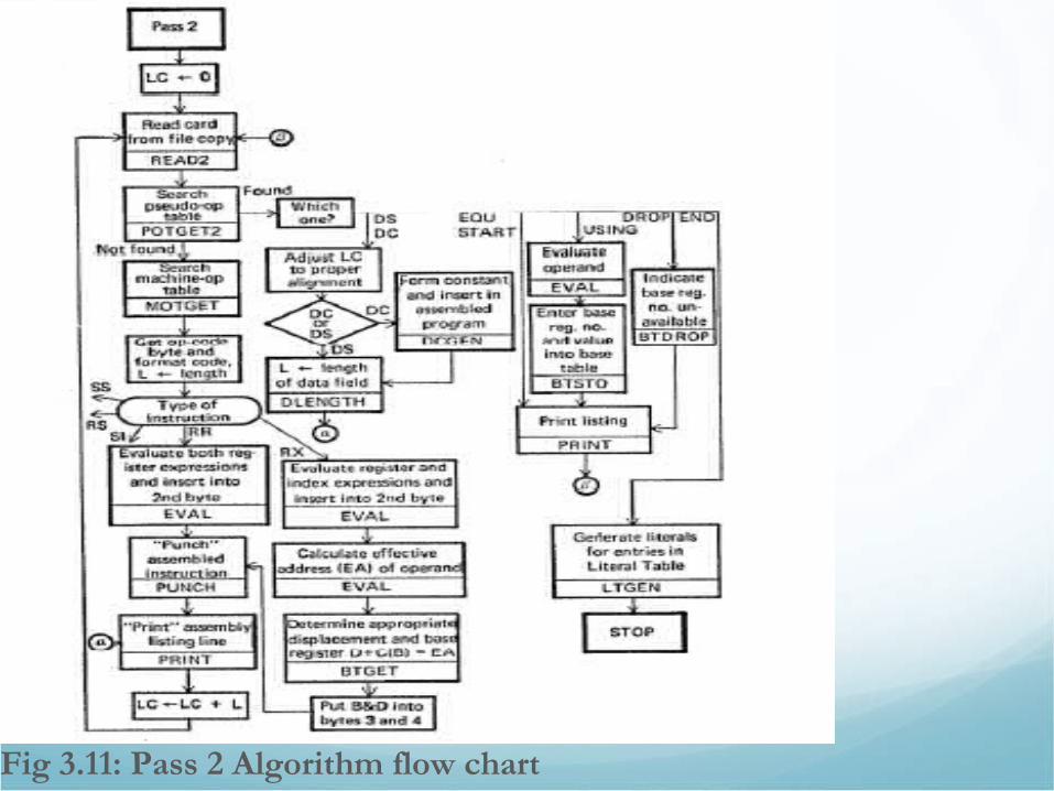
Fig 3.11: Pass 2 Algorithm flow chart

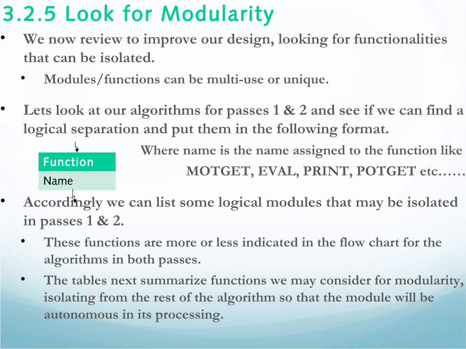
3.2.5 Look for Modularity• We now review to improve our design, looking for functionalities

that can be isolated. • Modules/functions can be multi-use or unique.

• Lets look at our algorithms for passes 1 & 2 and see if we can find a logical separation and put them in the following format.

Where name is the name assigned to the function like

MOTGET, EVAL, PRINT, POTGET etc……

• Accordingly we can list some logical modules that may be isolated in passes 1 & 2. • These functions are more or less indicated in the flow chart for the

algorithms in both passes.

• The tables next summarize functions we may consider for modularity, isolating from the rest of the algorithm so that the module will be autonomous in its processing.

Function

Name

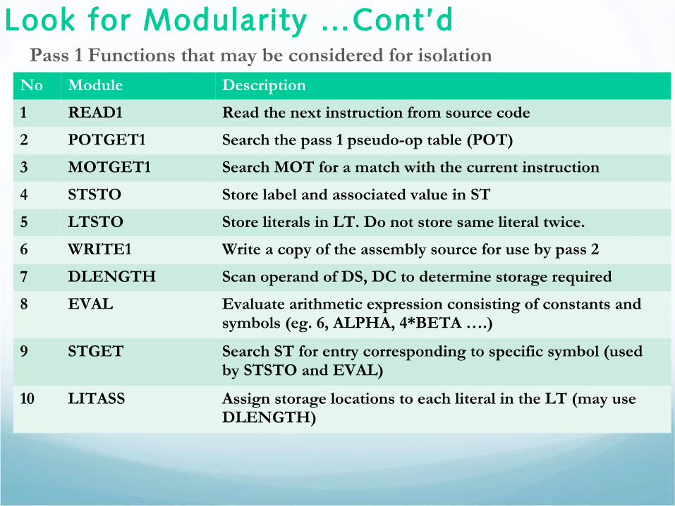
Look for Modularity …Cont’dPass 1 Functions that may be considered for isolation

No Module Description

1 READ1 Read the next instruction from source code

2 POTGET1 Search the pass 1 pseudo-op table (POT)

3 MOTGET1 Search MOT for a match with the current instruction

4 STSTO Store label and associated value in ST

5 LTSTO Store literals in LT. Do not store same literal twice.

6 WRITE1 Write a copy of the assembly source for use by pass 2

7 DLENGTH Scan operand of DS, DC to determine storage required

8 EVAL Evaluate arithmetic expression consisting of constants and symbols (eg. 6, ALPHA, 4*BETA ….)

9 STGET Search ST for entry corresponding to specific symbol (used by STSTO and EVAL)

10 LITASS Assign storage locations to each literal in the LT (may use DLENGTH)

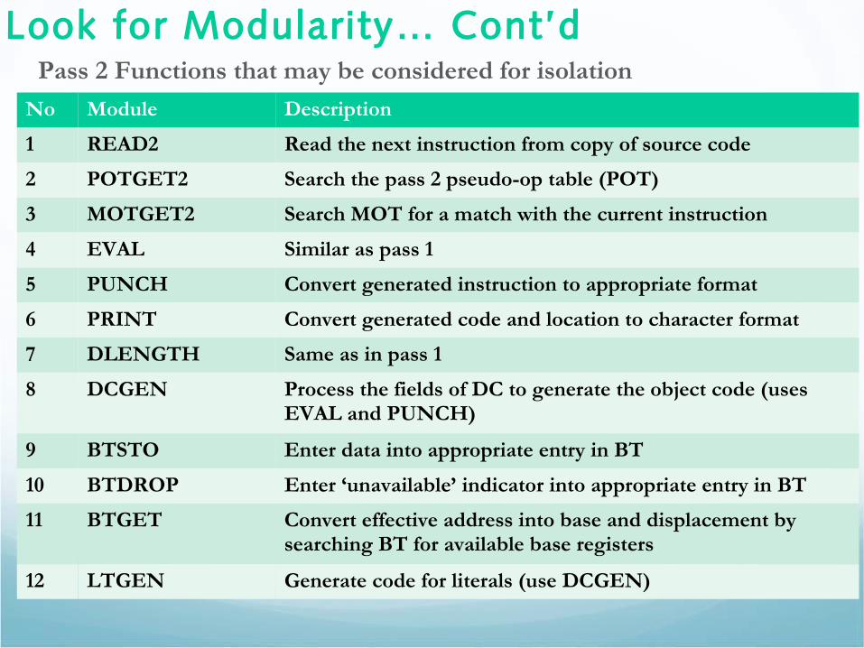
Look for Modularity… Cont’d Pass 2 Functions that may be considered for isolation

No Module Description

1 READ2 Read the next instruction from copy of source code

2 POTGET2 Search the pass 2 pseudo-op table (POT)

3 MOTGET2 Search MOT for a match with the current instruction

4 EVAL Similar as pass 1

5 PUNCH Convert generated instruction to appropriate format

6 PRINT Convert generated code and location to character format

7 DLENGTH Same as in pass 1

8 DCGEN Process the fields of DC to generate the object code (uses EVAL and PUNCH)

9 BTSTO Enter data into appropriate entry in BT

10 BTDROP Enter ‘unavailable’ indicator into appropriate entry in BT

11 BTGET Convert effective address into base and displacement by searching BT for available base registers

12 LTGEN Generate code for literals (use DCGEN)

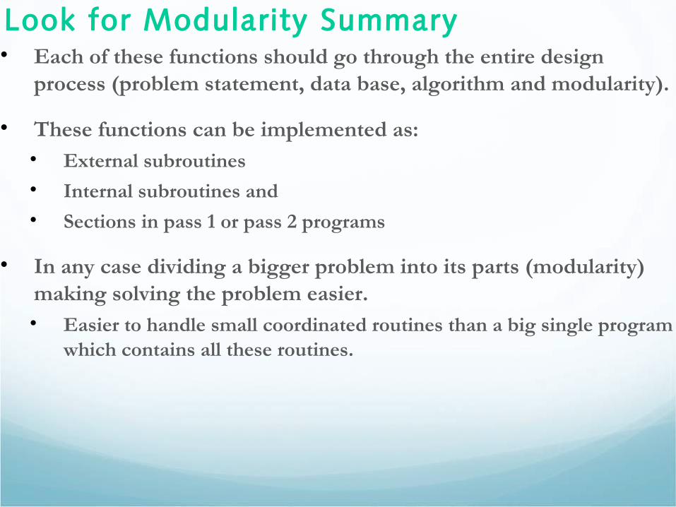
Look for Modularity Summary• Each of these functions should go through the entire design

process (problem statement, data base, algorithm and modularity).

• These functions can be implemented as:• External subroutines

• Internal subroutines and

• Sections in pass 1 or pass 2 programs

• In any case dividing a bigger problem into its parts (modularity) making solving the problem easier.• Easier to handle small coordinated routines than a big single program

which contains all these routines.

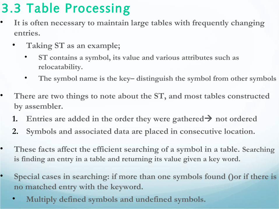
3.3 Table Processing• It is often necessary to maintain large tables with frequently changing

entries.

• Taking ST as an example;• ST contains a symbol, its value and various attributes such as

relocatability.

• The symbol name is the key– distinguish the symbol from other symbols

• There are two things to note about the ST, and most tables constructed by assembler.

1. Entries are added in the order they were gathered not ordered

2. Symbols and associated data are placed in consecutive location.

• These facts affect the efficient searching of a symbol in a table. Searching is finding an entry in a table and returning its value given a key word.

• Special cases in searching: if more than one symbols found ()or if there is no matched entry with the keyword.

• Multiply defined symbols and undefined symbols.

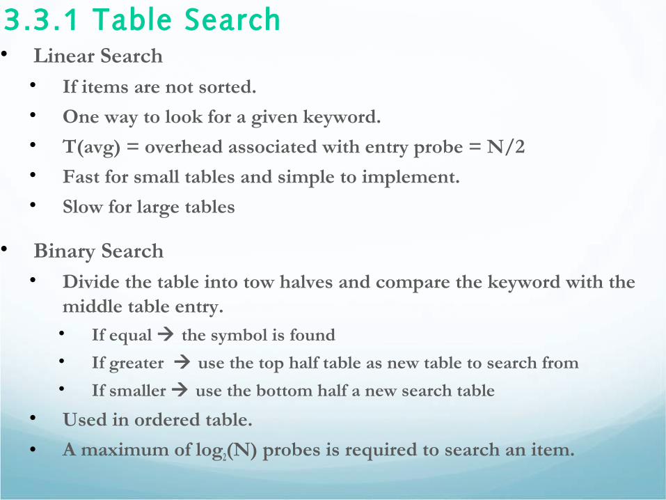
3.3.1 Table Search• Linear Search• If items are not sorted.

• One way to look for a given keyword.

• T(avg) = overhead associated with entry probe = N/2

• Fast for small tables and simple to implement.

• Slow for large tables

• Binary Search• Divide the table into tow halves and compare the keyword with the

middle table entry.• If equal the symbol is found

• If greater use the top half table as new table to search from

• If smaller use the bottom half a new search table

• Used in ordered table.

• A maximum of log2(N) probes is required to search an item.

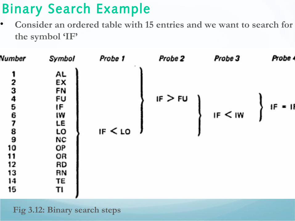
Binary Search Example• Consider an ordered table with 15 entries and we want to search for

the symbol ‘IF’

Fig 3.12: Binary search steps

Performance Comparison

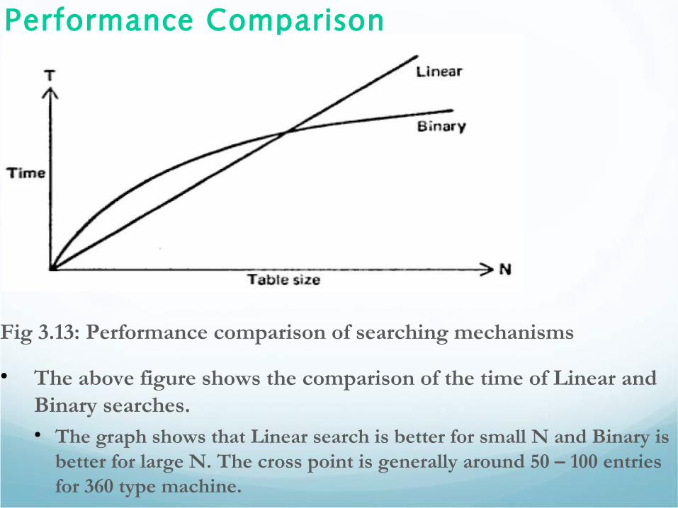
Fig 3.13: Performance comparison of searching mechanisms

• The above figure shows the comparison of the time of Linear and Binary searches.• The graph shows that Linear search is better for small N and Binary is

better for large N. The cross point is generally around 50 – 100 entries for 360 type machine.

3.3.2Sorting• For some purposes a Binary search is more efficient than Linear

search.• However such a search requires a sorted table, which may not be

always easy to obtain.

• The MOT and POT tables are fixed tables that can be manually organized to be ordered.

• However, this is not the case with none fixed tables like ST which are constructed by the assembler.• Entries are added into ST in the order they appear in the label of the

source code.

• Hence, sorting mechanisms and their efficiency should be considered in searching.• Some efficient search methods may employ less efficient sorting

mechanism that compromise the overall performance.

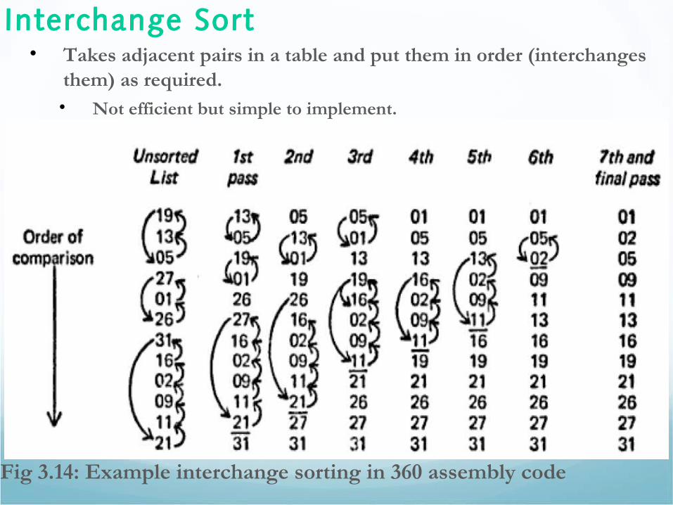
Interchange Sort• Takes adjacent pairs in a table and put them in order (interchanges

them) as required.• Not efficient but simple to implement.

Fig 3.14: Example interchange sorting in 360 assembly code

Shell Sort• Similar to INTERCHANGE SORT that it moves data by exchange.

• However, it begins by taking items in a distance ‘d’. Items that are away interchange quickly than simple INTERCHANGE SORT.• The value of ‘d’ is usually decreased in each pass.

• Shell sort approaches optimal performance for a comparative type of sort.

Bucket Sort

• Simple distributive sort also called radix sort. Sorting involves: • Examine least significant digit of the keyword first and place item into

uniquely identified bucket dependent on the digit.

• After all items are distributed, the buckets are merged in order.

• The process is repeated until no more digit is left.

• A number system of base P requires P buckets

End of Chapter Three!