assessing power plant cooling water intake system
TRANSCRIPT
ASSESSING POWER PLANT COOLING WATER INTAKE SYSTEM ENTRAINMENT IMPACTS
MARCH 2006
John R. Steinbeck1, John Hedgepeth1, Peter Raimondi2,
Gregor Cailliet3, and David L. Mayer4
1 – Tenera Environmental Inc., 141 Suburban Rd., Suite A2, San Luis Obispo, CA 93449
2 – Department of Ecology and Evolutionary Biology, University of California, Center for Ocean Health, Long Marine Lab, 100 Shaffer Road, Santa Cruz CA 95060
3 – Moss Landing Marine Laboratories, 8272 Moss Landing Rd., Moss Landing, CA 95039
4 – Tenera Environmental Inc., 971 Dewing Ave., Suite 100, Lafayette, CA 94539
DRAFT REPORT – For Information Purposes Only, Do NOT Cite or Reference
i
TABLE OF CONTENTS
LIST OF TABLES................................................................................................. ii LIST OF FIGURES .............................................................................................. iv EXECUTIVE SUMMARY ......................................................................................1 1.0 INTRODUCTION ...........................................................................................5 2.0 METHODS ...................................................................................................11
2.1 POWER PLANT DESCRIPTIONS ....................................................11 2.2 SOURCE WATER AND SOURCE POPULATION DEFINITIONS ....14 2.3 SAMPLING........................................................................................19 2.4 TARGET TAXA SELECTION ............................................................23 2.5 OTHER BIOLOGICAL DATA ............................................................27 2.6 PHYSICAL DATA COLLECTION ......................................................27 2.7 DATA REDUCTION ..........................................................................28 2.8 SOURCE WATER ESTIMATES........................................................31 2.9 IMPACT ASSESSMENT MODELS ...................................................32
3.0 RESULTS ....................................................................................................49 3.1 SOUTH BAY POWER PLANT ..........................................................49 3.2 MORRO BAY POWER PLANT .........................................................56 3.3 DIABLO CANYON POWER PLANT..................................................64
4.0 DISCUSSION...............................................................................................79 4.1 GUIDELINES FOR ENTRAINMENT IMPACT ASSESSMENT .........90 4.2 CONCLUSION ..................................................................................94
ACKNOWLEDGEMENTS ..................................................................................95 LITERATURE CITED .........................................................................................96 APPENDICES
A. Variance Calculations for FH, AEL, and ETM models B. Mean larval fish concentrations by station in San Diego Bay C. Estimates of CIQ goby larvae at SBPP used in calculating ETM
estimates of PE and annual estimate of proportional mortality (PM). D. Estimates of KGB rockfish larvae at MBPP used in calculating ETM
estimates of PE and annual estimate of proportional mortality (PM). E. Estimates of KGB rockfish larvae at DCPP used in calculating ETM
estimates of PE and annual estimate of proportional mortality (PM). F. Regression estimates, onshore and alongshore current meter
displacement, source water estimates, and estimates of the proportion of source water sampled (PS) used in calculating ETM for KGB rockfish larvae at DCPP.
DRAFT REPORT – For Information Purposes Only, Do NOT Cite or Reference
ii
LIST OF TABLES
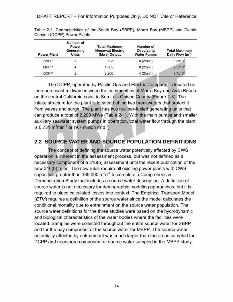
Table 2-1. Characteristics of the South Bay (SBPP), Morro Bay (MBPP) and Diablo Canyon (DCPP) Power Plants...........................................................14
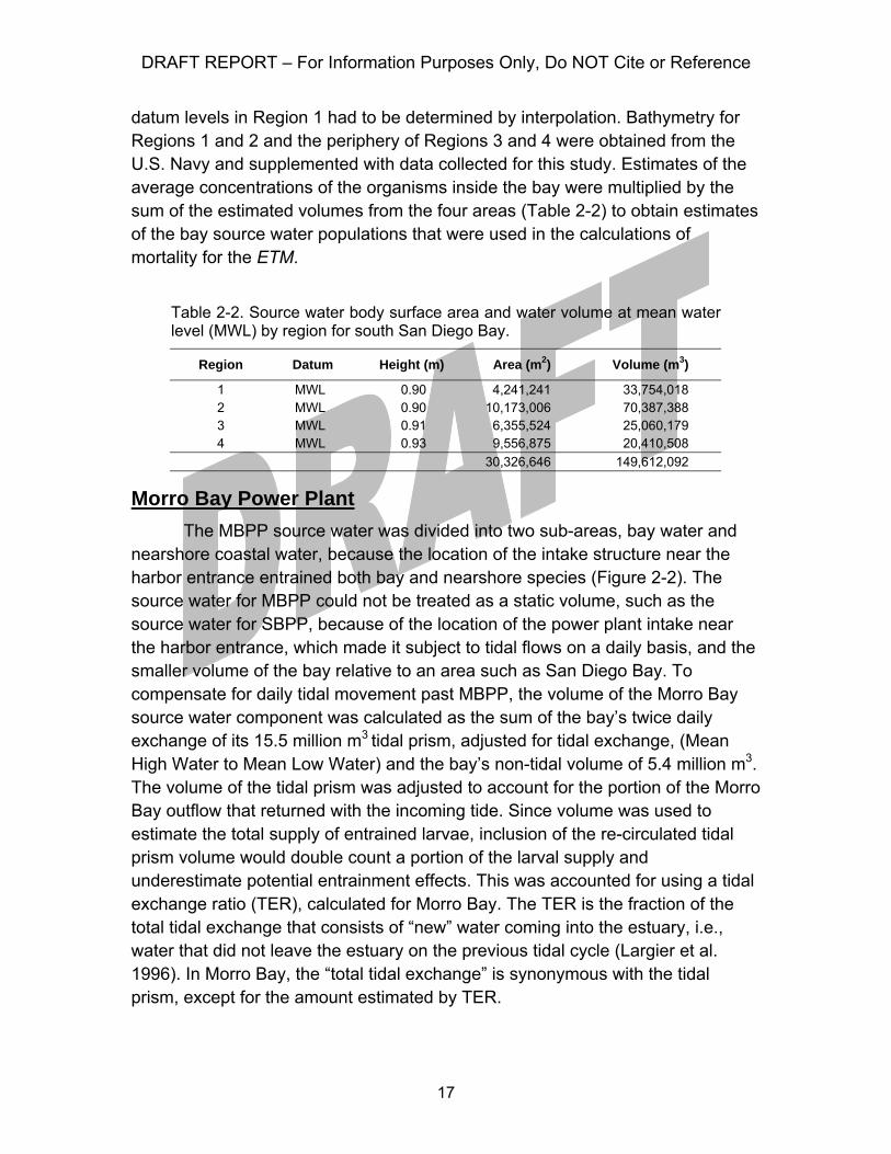
Table 2-2. Source water body surface area and water volume at mean water level (MWL) by region for south San Diego Bay. ..........................................17
Table 2-3. Volumes for Morro Bay and Estero Bay source water sub-areas. .....18 Table 2-4. Target taxa used in assessments at South Bay (SBPP), Morro Bay
(MBPP) and Diablo Canyon (DCPP) power plants. ......................................24 Table 2-5. Pigment groups of some preflexion rockfish larvae from Nishimoto (in-
prep). ............................................................................................................26 Table 3-1. Total annual entrainment estimates of larval fishes at South Bay
Power Plant.. ................................................................................................50 Table 3-2. Results of fecundity hindcasting (FH) modeling for CIQ goby complex
larvae entrained at South Bay Power Plant. .................................................53 Table 3-3. Results of adult equivalent loss (AEL) modeling for CIQ goby complex
larvae entrained at South Bay Power Plant. .................................................54 Table 3-4. Estimates of proportional entrainment (PE) and proportion of source
water population present for CIQ goby larvae at South Bay Power Plant entrainment and source water stations.........................................................55
Table 3-5. Summary of estimated South Bay Power Plant entrainment effects on target taxa. ...................................................................................................56
Table 3-6. Total annual entrainment estimates of fishes and target invertebrates at Morro Bay Power Plant.............................................................................57
Table 3-7. Annual estimates of adult female kelp, gopher, and black-and-yellow (KGB) rockfish losses at Morro Bay Power Plant based on larval entrainment estimates using the fecundity hindcasting (FH) model. ................................62
Table 3-8. Survival of the kelp, gopher, and black-and-yellow (KGB) rockfish complex larvae to an age of three years.......................................................62
Table 3-9. Annual estimates of adult kelp, gopher, and black-and-yellow (KGB) rockfish losses at Morro Bay Power Plant due to entrainment using the adult equivalent loss (AEL) model.........................................................................63
Table 3-10. Estimates of KGB rockfish larvae at MBPP entrainment and sourcewater stations.....................................................................................63
Table 3-11. Summary of estimated Morro Bay Power Plant entrainment effects on target taxa ...............................................................................................64

DRAFT REPORT – For Information Purposes Only, Do NOT Cite or Reference
iii
Table 3-12. Fishes collected during Diablo Canyon Power Plant entrainment sampling. ......................................................................................................65
Table 3-13. Diablo Canyon Power Plant entrainment estimates and standard errors for kelp, gopher, and black-and-yellow (KGB) rockfish complex.. ......68
Table 3-14. Diablo Canyon Power Plant fecundity hindcasting (FH) estimates for kelp, gopher, and black-and-yellow (KGB) rockfish complex........................72
Table 3-15. Diablo Canyon Power Plant adult equivalent loss (AEL) estimates for kelp, gopher, and black-and-yellow (KGB) rockfish complex. .................73
Table 3-16. Estimates used in calculating empirical transport model (ETM) estimates of proportional entrainment (PE) for kelp, gopher, and black-and-yellow (KGB) rockfish complex for Diablo Canyon Power Plant. ..................75
Table 3-17. Onshore and alongshore current meter displacement measurements used in estimating proportion of source water sampled (PS) ........................76
Table 3-18. Results of entrainment monitoring and FH, AEL, and ETM modeling for fourteen fishes at Diablo Canyon Power Plant. ......................................78
DRAFT REPORT – For Information Purposes Only, Do NOT Cite or Reference
iv
LIST OF FIGURES
Figure 1-1. Conceptual diagram of power plant cooling water systems at Morro Bay, Diablo Canyon, and South Bay Power Plants. .......................................6
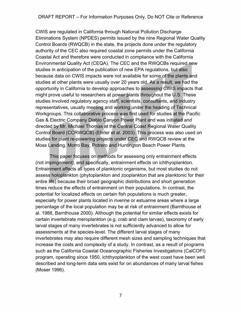
Figure 1-2. Locations of Morro Bay (MBPP), Diablo Canyon (DCPP), and South Bay Power Plants (SBPP). ...........................................................................10
Figure 2-1. Location of South Bay Power Plant entrainment (SB01) and source water stations and detail of power plant intake area.....................................12
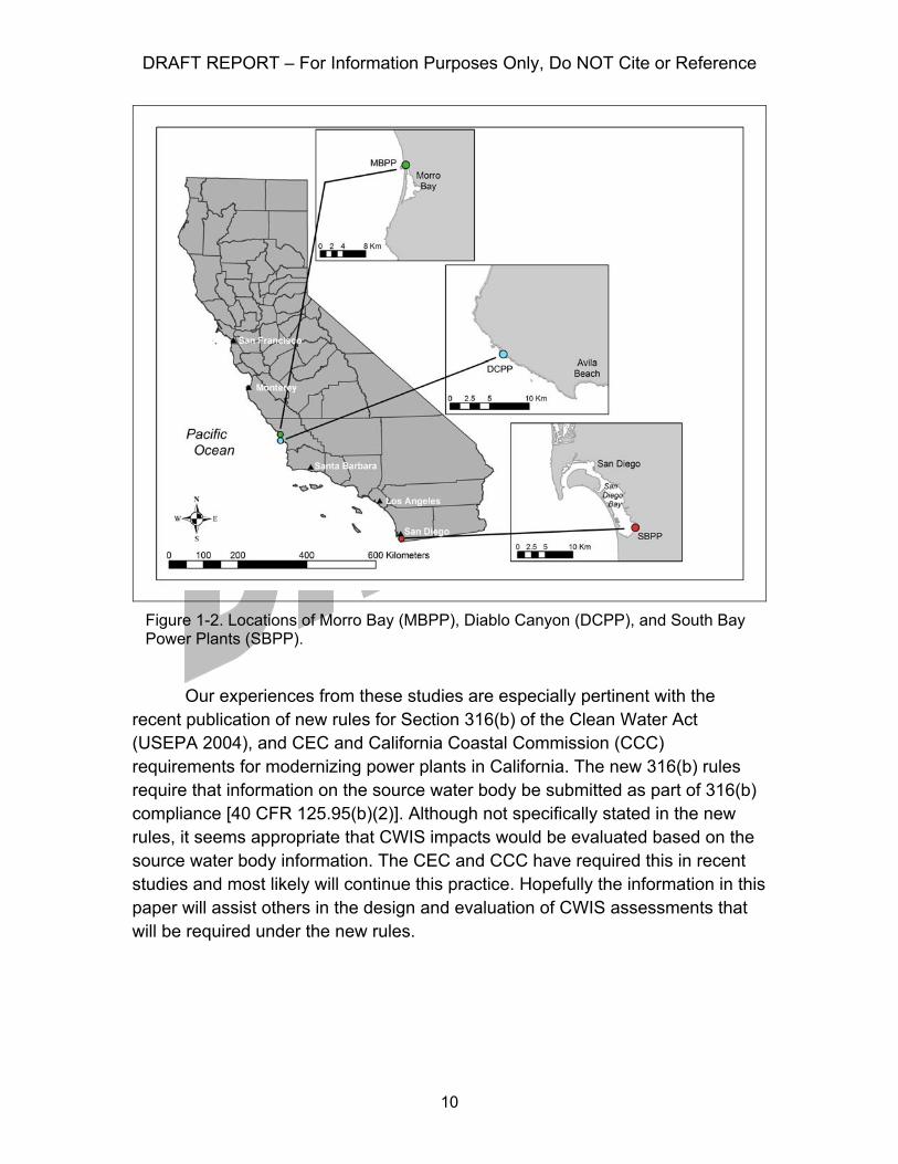
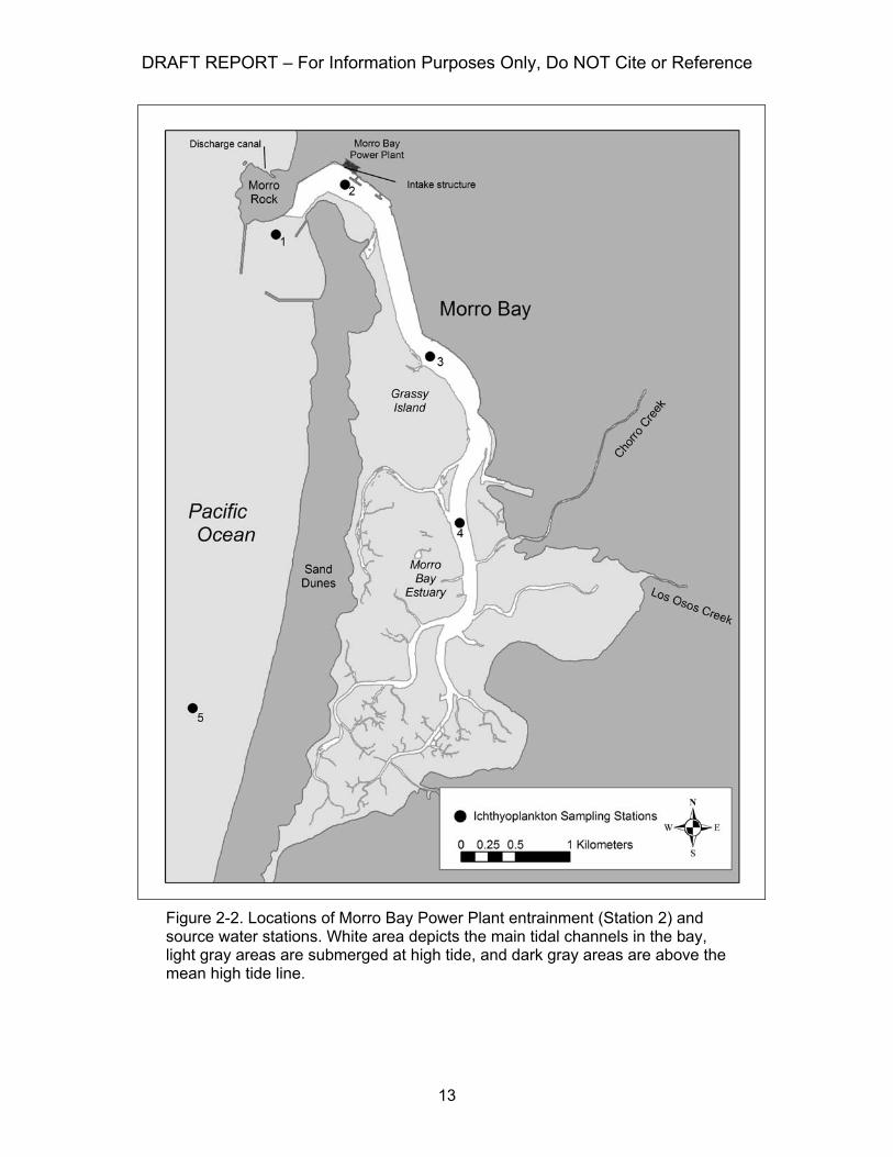
Figure 2-2. Locations of Morro Bay Power Plant entrainment (Station 2) and source water stations....................................................................................13
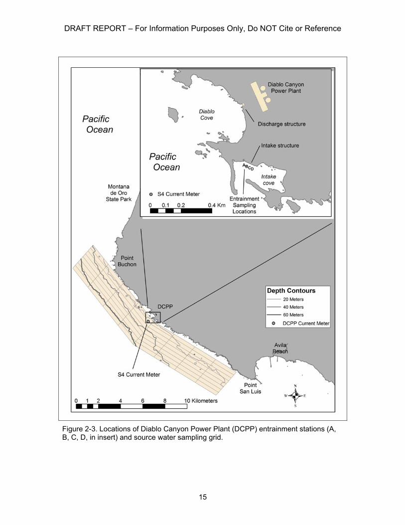
Figure 2-3. Locations of Diablo Canyon Power Plant (DCPP) entrainment stations and source water sampling grid. .....................................................15
Figure 2-4. Relative cumulative upcoast/downcast and onshore/offshore current vectors west of the Diablo Canyon Power Plant. ..........................................47
Figure 3-1. Monthly mean larval concentration of the CIQ goby complex larvae at SBPP............................................................................................................51
Figure 3-2. Length frequency distribution for Clevlandia ios, Ilypnus gilberti, and Quietula y-cauda (CIQ) goby complex larvae from the SBPP entrainment station...........................................................................................................52
Figure 3-3. Weekly mean larval concentration of kelp, gopher, and black-and-yellow (KGB) rockfish complex larvae at the MBPP intake entrainment station...........................................................................................................59
Figure 3-4. Comparison of average concentrations of kelp, gopher, and black-and-yellow (KGB) rockfish complex larvae at the Morro Bay Power Plant intake, Morro Bay, and Estero Bay. ..............................................................60
Figure 3-5. Length frequency distribution for kelp, gopher, and black-and-yellow (KGB) rockfish complex larvae from the MBPP entrainment station.............61
Figure 3-6. Weekly mean larval concentrations of kelp, gopher, and black-and-yellow (KGB) rockfish complex larvae at the DCPP intake entrainment stations.. .......................................................................................................67
Figure 3-7. Annual mean concentration for kelp, gopher, and black-and-yellow (KGB) rockfish complex larvae collected from surface plankton tows in DCPP Intake Cove. .................................................................................................68
Figure 3-8. Average concentration for kelp, gopher, and black-and-yellow (KGB) rockfish complex larvae in each of the 64 nearshore stations for DCPP ......70
Figure 3-9. Length frequency distribution for kelp, gopher, and black-and-yellow (KGB) rockfish complex larvae measured from entrainment stations at DCPP intake............................................................................................................71

DRAFT REPORT – For Information Purposes Only, Do NOT Cite or Reference
1
EXECUTIVE SUMMARY
Steam electric power plants and other industries that withdraw cooling water from surface water bodies are regulated in the U.S. under Section 316(b) of the Clean Water Act of 1972. Of the industries regulated under section 316(b), steam electric power plants have the largest cooling water volumes with some large plants exceeding two billion gallons per day. Environmental effects of cooling water withdrawal result from impingement of larger organisms on screens that block material from entering the cooling water system and the entrainment of smaller organisms into and through the system. The assessment of impingement effects is relatively straightforward. This report focuses on the assessment of entrainment effects.
The difficulties in entrainment assessments arise from several factors. The organisms entrained include planktonic larvae of fishes and invertebrates that are difficult to sample and identify. The entrained larvae are also part of larger source water populations that may extend over large areas or be confined to limited habitats making it difficult to determine the effects of entrainment losses. The early life histories of most fishes on the Pacific coast are also poorly described limiting the usefulness of demographic models for assessing entrainment effects. All of these factors make the assessment of cooling water system entrainment difficult.
This report describes three studies for assessing entrainment at coastal power plants in California. They represent a range of marine and estuarine habitats: the South Bay Power Plant in south San Diego Bay, and the Morro Bay and Diablo Canyon Power Plants in central California. These studies utilized a multiple modeling approach for assessing entrainment effects. When appropriate life history information was available for a species, demographic modeling techniques were used to calculate the numbers of adults represented by the entrainment losses. The primary approach for assessment at these plants was the Empirical Transport Model (ETM), originally developed for use with power plants entraining water from rivers, and then adapted for use on the open coast and in estuaries in southern California. The ETM utilizes the same principles used in fishery management to estimate effects of fishing mortality on the sustainability of a stock. Just as fishery managers use catch and population size to estimate fishery mortality, the ETM requires estimates of both entrainment and source water larval populations. The process of defining the source water and obtaining an estimate of its population varied among the three plants and also among species within studies. The purpose of this paper is to present the
DRAFT REPORT – For Information Purposes Only, Do NOT Cite or Reference
2
multiple modeling approaches used for power plant entrainment assessments, with the main focus being a comparison of the processes used to define the source water populations used in the ETM modeling from the three power plants.
The results showed that the standard demographic models were generally not usable with species found along the California coast due to the absence of life history information for most of them. The results for the ETM ranged from very small levels (<1.0%) of proportional mortality due to entrainment for wide ranging pelagic species such as northern anchovy to levels as high as 50% for species with more limited habitat that were spawned near power plant intake structures. The results of the ETM were generally consistent with the biology and habitat distributions of the fishes analyzed.
Based on our experiences with these and other studies we believe that a prescriptive approach to the design of entrainment assessments is not possible, and therefore, we provide some general considerations that might be helpful in the design, sampling, and analysis of entrainment impact assessments.
During the design of the study ensure that potential target species that could be affected by entrainment are effectively sampled and insure that the sampling will account for any endangered, threatened, or other listed species that could be affected by entrainment. In addition to identifying species potentially affected, it is critical to determine the source water areas potentially affected including the distribution of habitats that might be differentially affected by CWIS entrainment. The sampling plan also needs to account for the design, location, and hydrodynamics of the power plant intake structure. The sampling frequency should accommodate important species that might have short spawning seasons. This may require that the sampling frequency be seasonally adjusted based on presence of certain species. The relative effects of entrainment estimated by the ETM model should be much less subject to interannual variation than absolute estimates using FH, AEL or other demographic models. Therefore, if source water sampling is done in conjunction with entrainment sampling then one year is a reasonable period of sampling for these studies. The size of the source water sampling area should be based on the hydrodynamics of the system. In a closed system this may be the entire source water. In an open system, ocean or tidal currents and dispersion should be used to determine the appropriate sampling area for estimating daily entrainment mortality (PE) for the larger source water population.
Some practical considerations for sample collection and processing include adjusting the sample volume for the larval concentrations in the source
DRAFT REPORT – For Information Purposes Only, Do NOT Cite or Reference
3
waters. This is best done using preliminary sampling with the gear proposed for the study. Age of larvae are best determined using analysis of otoliths, but if this is not possible be sure that length frequencies measured from the entrainment samples are realistic based on available life history and account for egg stages that would be subject to entrainment if fish eggs are not sorted and identified from the samples. This is easily accommodated in the ETM approach by adding the duration of the planktonic egg stage to the larval duration calculated from the otolith or length data.
Although we believe that the ETM is best approach for assessment, results from multiple models provide additional information for verifying results and for determining effects at the adult population level. One approach for assessment at the adult population level is through converting ETM results into an estimate of the habitat necessary to replace the production lost due to entrainment (Area of Production Foregone [APF]). The APF is calculated by multiplying the area of habitat present within the estimated source water by the proportional entrainment mortality estimated from ETM. This approach may be useful for scaling restoration projects to help offset losses due to entrainment. The ETM can also be used to estimate the number of equivalent adults lost by entrainment by applying the mortality estimate to a survey of the standing stock. This can be compared with estimates from FH and AEL. It is also useful in these types of comparisons to hindcast or extrapolate the FH and AEL models to the same age. This may not necessarily result in the same estimates from both models unless the data used in the two models are derived from a life table assuming a stable age distribution. The USEPA (2002) used AEL and another demographic modeling approach, production foregone, to estimate the number of age-1 individuals lost due to power plant impingement and entrainment. The accuracy of estimates from any of these demographic models is subject to the underlying uncertainty in aging, survival, and fecundity estimates and population regulatory, behavioral, or environmental factors that may be operating on the subject populations at the time the life history data were collected.
Uncertainty associated with the ETM is primarily derived from sampling error that can be controlled by careful design using some of the guidelines provided in this report. With a good sampling design, the ETM provides a site-specific, empirically based approach to entrainment assessment that is a major improvement over demographic modeling approaches. In addition, the results can be used to estimate entrainment effects on other planktonic organisms that are not the target of the analysis, in estimating cumulative effects of multiple power plants and other sources of mortality, and in scaling restoration efforts to offset losses due to entrainment. We hope that the information in this report will

DRAFT REPORT – For Information Purposes Only, Do NOT Cite or Reference
4
assist others in the design and analysis of CWIS assessments that will be required as a result of the recent publication of new rules for Section 316(b) of the Clean Water Act (USEPA 2004).
DRAFT REPORT – For Information Purposes Only, Do NOT Cite or Reference
5
1.0 INTRODUCTION
Steam electric power plants and other industries (e.g., pulp and paper, iron and steel, chemical, manufacturing, petroleum refineries, and oil and gas production) use water from coastal areas for cooling resulting in impacts to the marine organisms occupying the affected water bodies. Industries that withdraw cooling water from surface water bodies are regulated in the U.S. under Section 316(b) of the Clean Water Act of 1972 [33 U.S. Code Section 1326(b)]. Section 316(b) requires “…that the location, design, construction, and capacity of cooling water intake structures reflect the best technology available for minimizing adverse environmental impacts.” Of the industries regulated under section 316(b), steam electric power plants have the largest cooling water volumes ranging from tens of thousands to millions of m
3 d
-1
(Veil et al. 2003). A survey in 1996 reported that 44% of the power plants in the U.S. utilized a steam electric process involving once-through cooling (Veil 2000). Electricity is generated at these plants by heating purified water to create high-pressure steam, which is expanded in turbines that drive generators and produce electricity (Figure 1-1). After leaving the turbines, steam passes through a condenser where high volume cooling water flow cools and condenses the steam, which is then re-circulated back through the system.
Regulatory guidance for complying with section 316(b), that was first proposed by the U.S. Environmental Protection Agency (EPA) in 1976, was successfully challenged in the courts by a group of 58 utility companies in 1977 and never implemented (Bulleit 2000). As a result, section 316(b) was implemented by the states using a broad range of approaches; some states developed fairly comprehensive programs while others never adopted any formal regulations (Veil et al. 2003). The EPA has recently published new regulations for 316(b) compliance as part of the settlement of a lawsuit against the EPA by environmental groups headed by the Hudson Riverkeeper (Nagle and Morgan 2000). As a result of these new regulations power plants throughout the U.S. are now required to reduce the environmental effects of their cooling water intake systems (CWIS).
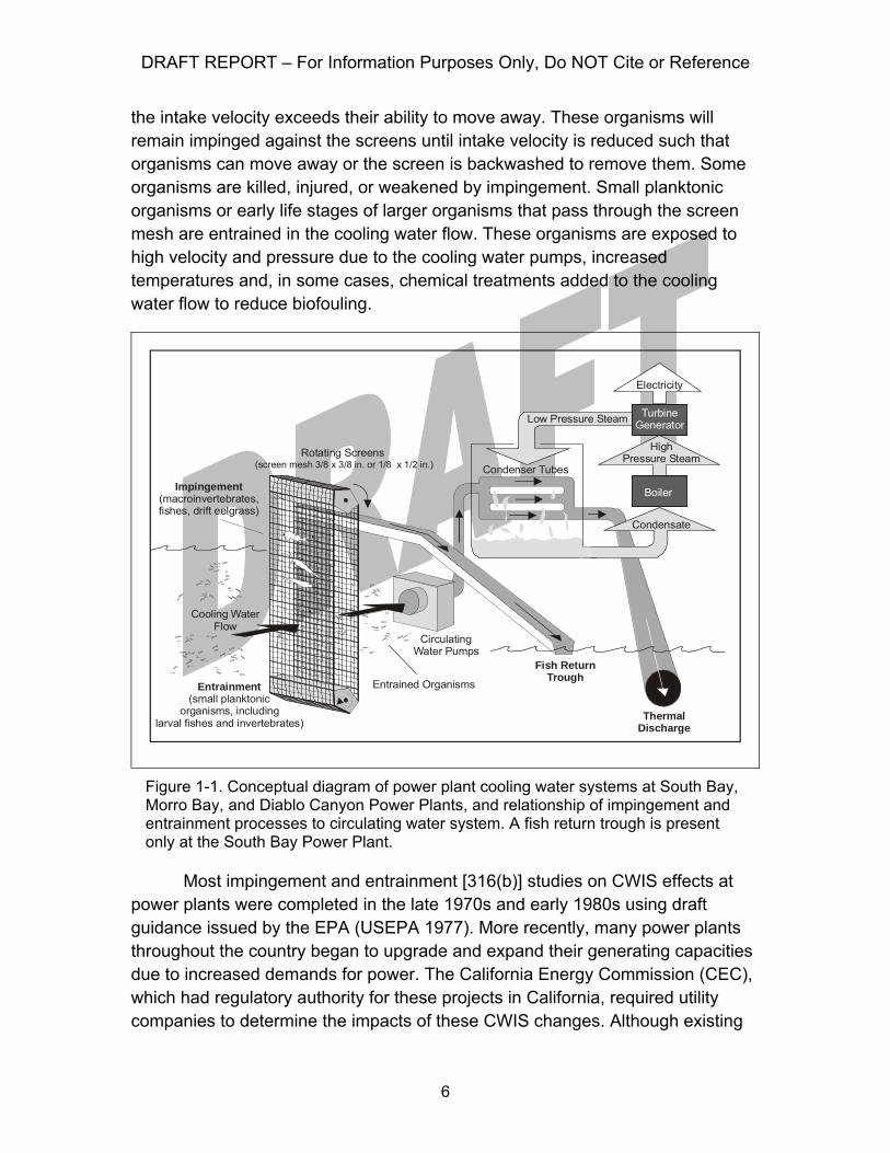
The withdrawal of water by once-through cooling water systems has two major impacts on the biological organisms in the source water body: impingement and entrainment (Figure 1-1). Almost all power plants with once-through cooling employ some type of screening device to block large objects from entering the cooling water system (impingement). Fishes and other aquatic organisms large enough to be blocked by the screens may become impinged if
DRAFT REPORT – For Information Purposes Only, Do NOT Cite or Reference
6
the intake velocity exceeds their ability to move away. These organisms will remain impinged against the screens until intake velocity is reduced such that organisms can move away or the screen is backwashed to remove them. Some organisms are killed, injured, or weakened by impingement. Small planktonic organisms or early life stages of larger organisms that pass through the screen mesh are entrained in the cooling water flow. These organisms are exposed to high velocity and pressure due to the cooling water pumps, increased temperatures and, in some cases, chemical treatments added to the cooling water flow to reduce biofouling.
Most impingement and entrainment [316(b)] studies on CWIS effects at power plants were completed in the late 1970s and early 1980s using draft guidance issued by the EPA (USEPA 1977). More recently, many power plants throughout the country began to upgrade and expand their generating capacities due to increased demands for power. The California Energy Commission (CEC), which had regulatory authority for these projects in California, required utility companies to determine the impacts of these CWIS changes. Although existing
Low Pressure Steam
CirculatingWater Pumps
Impingement(macroinvertebrates, fishes, drift eelgrass)
Entrainment(small planktonic
organisms, includinglarval fishes and invertebrates)
Entrained Organisms
Cooling Water Flow
Fish Return Trough
Thermal Discharge
Condenser Tubes
Condensate
High Pressure Steam
Electricity
Rotating Screens (screen mesh 3/8 x 3/8 in. or 1/8 x 1/2 in.)
Boiler
Turbine Generator
Figure 1-1. Conceptual diagram of power plant cooling water systems at South Bay, Morro Bay, and Diablo Canyon Power Plants, and relationship of impingement and entrainment processes to circulating water system. A fish return trough is present only at the South Bay Power Plant.
DRAFT REPORT – For Information Purposes Only, Do NOT Cite or Reference
7
CWIS are regulated in California through National Pollution Discharge Eliminations System (NPDES) permits issued by the nine Regional Water Quality Control Boards (RWQCB) in the state, the projects done under the regulatory authority of the CEC also required coastal zone permits under the California Coastal Act and therefore were conducted in compliance with the California Environmental Quality Act (CEQA). The CEC and the RWQCBs required new studies in anticipation of the publication of new EPA regulations, but also because data on CWIS impacts were not available for some of the plants and studies at other plants were usually over 20 years old. As a result, we had the opportunity in California to develop approaches to assessing CWIS impacts that might prove useful to researchers at power plants throughout the U.S. These studies involved regulatory agency staff, scientists, consultants, and industry representatives, usually meeting and working under the heading of Technical Workgroups. This collaborative process was first used for studies at the Pacific Gas & Electric Company Diablo Canyon Power Plant and was initiated and directed by Mr. Michael Thomas at the Central Coast Regional Water Quality Control Board (CCRWQCB) (Ehrler et al. 2003). This process was also used on studies for plant re-powering projects under CEC and RWQCB review at the Moss Landing, Morro Bay, Potrero and Huntington Beach Power Plants.
This paper focuses on methods for assessing only entrainment effects (not impingement), and specifically, entrainment effects on ichthyoplankton. Entrainment affects all types of planktonic organisms, but most studies do not assess holoplankton (phytoplankton and zooplankton that are planktonic for their entire life) because their broad geographic distributions and short generation times reduce the effects of entrainment on their populations. In contrast, the potential for localized effects on certain fish populations is much greater, especially for power plants located in riverine or estuarine areas where a large percentage of the local population may be at risk of entrainment (Barnthouse et al. 1988, Barnthouse 2000). Although the potential for similar effects exists for certain invertebrate meroplankton (e.g. crab and clam larvae), taxonomy of early larval stages of many invertebrates is not sufficiently advanced to allow for assessments at the species-level. The different larval stages of many invertebrates may also require different mesh sizes and sampling techniques that increase the costs and complexity of a study. In contrast, as a result of programs such as the California Coastal Oceanographic Fisheries Investigations (CalCOFI) program, operating since 1950, ichthyoplankton of the west coast have been well described and long-term data sets exist for on abundances of many larval fishes (Moser 1996).

DRAFT REPORT – For Information Purposes Only, Do NOT Cite or Reference
8
The best-documented and most extensive 316(b) studies from the period of the late 1970s and early 1980s were from the Hudson River power plants (Barnthouse et al. 1988, Barnthouse 2000). Impacts of cooling water withdrawals from three plants were extensively studied using long-term, river-wide sampling and analyzed using mathematical models designed to predict the effects on striped bass and other fish populations. After many years of debate surrounding a lawsuit, the case was settled out of court. Two of the most important factors in laying the groundwork for the settlement were the converging estimates of the effects from different researchers and the development of models that estimated conditional mortality from empirical data that reflected the “complex interactions of a host of factors” and helped identify the “relative importance of each component of the analysis” (Englert and Boreman 1988).
Numerous demographic modeling approaches have been proposed and used for projecting losses from CWIS impacts (Dey 2003). Equivalent adult (Horst 1975, Goodyear 1978), production foregone (Rago 1984), and variations of these approaches and models (Dey 2003) translate entrainment losses of egg and larval stages into equivalent units (adult fishes, biomass, etc.) that otherwise would not have been lost to the population. Although these models are the most commonly used methods for CWIS assessment and are recommended for use by the EPA in their new 316(b) rules (USEPA 2004), there are problems with their application and interpretation. The models require life history parameters (larval duration, survival, fecundity, etc.) that are available for only a limited number of species, generally those managed for commercial or recreational fishing. Our experience has shown that on the California coast, species that are usually entrained in highest numbers are small, forage species that have very limited life history information available.
However, these models are attractive because their interpretation appears to be straightforward since they convert larval forms into “equivalent units” that are more easily understood by the public, regulators, and managers. The estimates of numbers or biomass of fish from the models can also be added to losses from impingement and compared with commercial or recreational fishery data to provide cost estimates of the losses. Unfortunately, these interpretations are available for only a few species, there is usually no scale for determining the significance of the losses to the source water populations, and the studies are only done for a 1-2 yr period. As a result, the studies do not account for inter-annual variation in larval abundances.
Our assessments included a modified version of the Empirical Transport Model (ETM) (Boreman et al. 1978, 1981) which circumvented the problems with

DRAFT REPORT – For Information Purposes Only, Do NOT Cite or Reference
9
existing demographic modeling. This model was first developed for use with power plants entraining water from rivers, but MacCall et al. (1983) used the same general approach for entrainment assessments at power plants on the open coast and in estuaries in southern California. In contrast to demographic models, it does not require detailed life history information. The ETM is based on the same principles used in fishery management to estimate effects of fishing mortality on the sustainability of a stock (Boreman et al. 1981, MacCall et al. 1983). The conditional entrainment rate estimated by ETM is analogous to conditional fishing mortality as defined by Ricker (1975). Inherent in this approach is the requirement for an estimate of the source water population affected by entrainment. Although not specifically required for calculating estimated losses, an estimate of the source water population is also required to provide a context for the losses estimated by demographic models.
The process of defining the source water and obtaining an estimate of its population varies among studies and also among species within studies. The purpose of this paper is to present the multiple modeling approaches used for power plant entrainment assessments, with the main focus being a comparison of the processes used to define the source water populations used in the ETM modeling from three power plants in California, South Bay Power Plant (SBPP), Morro Bay Power Plant (MBPP), and Diablo Canyon Power Plant (DCPP), which represent a range of marine and estuarine habitats (Figure 1-2). This comparison allows us to compare the approaches and assess the influence of the source water on the proportional mortality of affected fish and invertebrate larval taxa.
The source water for SBPP, located in south San Diego Bay estuary, was defined as a closed system, while the source water for another estuarine study in Morro Bay, San Luis Obispo County at MBPP was defined as an semi-open system due to exchange with nearshore coastal waters. The studies at these two estuarine sites are compared with a study at DCPP, located on the open coast in central California, where the source water was defined as an open system. The many factors that need to be considered in the design of these studies can be examined by comparing the different approaches taken at these three facilities.
During the course of these studies we have modified the assessment approaches and this process has continued as we have participated in additional, more recent studies. Therefore one of the additional purposes of this paper is to present these more recent changes in our assessment methods even though they may differ from the methods presented for the three example studies.
DRAFT REPORT – For Information Purposes Only, Do NOT Cite or Reference
10
Figure 1-2. Locations of Morro Bay (MBPP), Diablo Canyon (DCPP), and South Bay Power Plants (SBPP).
Our experiences from these studies are especially pertinent with the recent publication of new rules for Section 316(b) of the Clean Water Act (USEPA 2004), and CEC and California Coastal Commission (CCC) requirements for modernizing power plants in California. The new 316(b) rules require that information on the source water body be submitted as part of 316(b) compliance [40 CFR 125.95(b)(2)]. Although not specifically stated in the new rules, it seems appropriate that CWIS impacts would be evaluated based on the source water body information. The CEC and CCC have required this in recent studies and most likely will continue this practice. Hopefully the information in this paper will assist others in the design and evaluation of CWIS assessments that will be required under the new rules.
DRAFT REPORT – For Information Purposes Only, Do NOT Cite or Reference
11
2.0 METHODS
2.1 POWER PLANT DESCRIPTIONS The studies we will be presenting as examples were conducted at three
power plants: SBPP, MBPP, and DCPP (Figure 1-2). The CWIS for all three plants share several features: shoreline intake structures with stationary trash racks that consist of vertical steel bars to prevent larger objects and organisms from entering the system and traveling water screens (TWS) located behind the bar racks that screen out smaller organisms and debris from the system (Figure 1-1).
Entrainment occurs to organisms that pass through the smaller mesh of the TWS. These organisms are exposed to increased temperatures and pressures as they pass through CWS. The surfaces of the piping in the CWS can be covered with biofouling organisms that feed on organisms that pass through the system. Although studies have shown that there may be some survival after CWS passage (Mayhew et al. 2000), most of these studies were conducted at power plants in rivers and estuaries on the east coast or in the Gulf of Mexico where biofouling was not recognized as a large problem compared with coastal environments. In addition, these studies only examined survival after passage through the system, and did not include comparisons of intake and discharge concentrations where losses due to cropping should be factored into CWS survival. For these reasons, our assessments of CWS effects have assumed that entrained organisms experience 100% mortality.
The SBPP, operated by Duke Energy, is located on the southeastern shore of San Diego Bay in the city of Chula Vista, California, approximately 16 km north of the U. S. − Mexican border (Figure 2-1). The plant draws water from San Diego Bay for once-through cooling of its four electric generating units, which can produce a maximum of 723 MWe (Table 2-1). With all pumps in operation, maximum water flow through the plant is 1,580 m3min-1 (2.3 million m3d-1).
The MBPP, operated by Duke Energy, is located on the northeastern shoreline of Morro Bay, which is approximately midway between San Francisco and Los Angeles, California (Figure 2-2). The plant draws water from Morro Bay for once-through cooling of its four electric generating units, which can produce a total of 1,002 MWe (Table 2-1). With all pumps in operation, water flow through the plant is 1,756 m3min-1 (2.53 million m3d-1). Morro Bay studies were done as part of the permitting requirements for an upgrade to the plant that result in a

DRAFT REPORT – For Information Purposes Only, Do NOT Cite or Reference
12
decrease in flow to 1,086 m3min-1 (1.56 million m3d-1). Therefore, all of the entrainment estimates and modeling were calculated using this flow rate.
Figure 2-1. Location of South Bay Power Plant entrainment (SB01) and source water stations and detail of power plant intake area. Shaded areas represent regions of the bay used in calculating bay volumes.
DRAFT REPORT – For Information Purposes Only, Do NOT Cite or Reference
13
Figure 2-2. Locations of Morro Bay Power Plant entrainment (Station 2) and source water stations. White area depicts the main tidal channels in the bay, light gray areas are submerged at high tide, and dark gray areas are above the mean high tide line.
DRAFT REPORT – For Information Purposes Only, Do NOT Cite or Reference
14
Table 2-1. Characteristics of the South Bay (SBPP), Morro Bay (MBPP) and Diablo Canyon (DCPP) Power Plants.
Power Plant
Number of Power
Generating Units
Total Maximum Megawatt Electric
(Mwe) Output
Number of Circulating
Water Pumps Total Maximum Daily Flow (m3)
SBPP 4 723 8 (2/unit) 2.3x10⁶
MBPP 4 1,002 8 (2/unit) 2.5x10⁶
DCPP 2 2,200 4 (2/unit) 9.7x10⁶
The DCPP, operated by Pacific Gas and Electric Company, is located on the open coast midway between the communities of Morro Bay and Avila Beach on the central California coast in San Luis Obispo County (Figure 2-3). The intake structure for the plant is located behind two breakwaters that protect it from waves and surge. The plant has two nuclear-fueled generating units that can produce a total of 2,200 MWe (Table 2-1). With the main pumps and smaller auxiliary seawater system pumps in operation, total water flow through the plant is 6,731 m3min-1 or (9.7 million m3d-1).
2.2 SOURCE WATER AND SOURCE POPULATION DEFINITIONS The concept of defining the source water potentially affected by CWS
operation is inherent in the assessment process, but was not defined as a necessary component of a 316(b) assessment until the recent publication of the new 316(b) rules. The new rules require all existing power plants with CWS capacities greater than 189,000 m3d-1 to complete a Comprehensive Demonstration Study that includes a source water description. A definition of source water is not necessary for demographic modeling approaches, but it is required to place calculated losses into context. The Empirical Transport Model (ETM) requires a definition of the source water since the model calculates the conditional mortality due to entrainment on the source water population. The source water definitions for the three studies were based on the hydrodynamic and biological characteristics of the water bodies where the facilities were located. Samples were collected throughout the entire source water for SBPP and for the bay component of the source water for MBPP. The source water potentially affected by entrainment was much larger than the areas sampled for DCPP and nearshore component of source water sampled in the MBPP study.
DRAFT REPORT – For Information Purposes Only, Do NOT Cite or Reference
15
Figure 2-3. Locations of Diablo Canyon Power Plant (DCPP) entrainment stations (A, B, C, D, in insert) and source water sampling grid.
DRAFT REPORT – For Information Purposes Only, Do NOT Cite or Reference
16
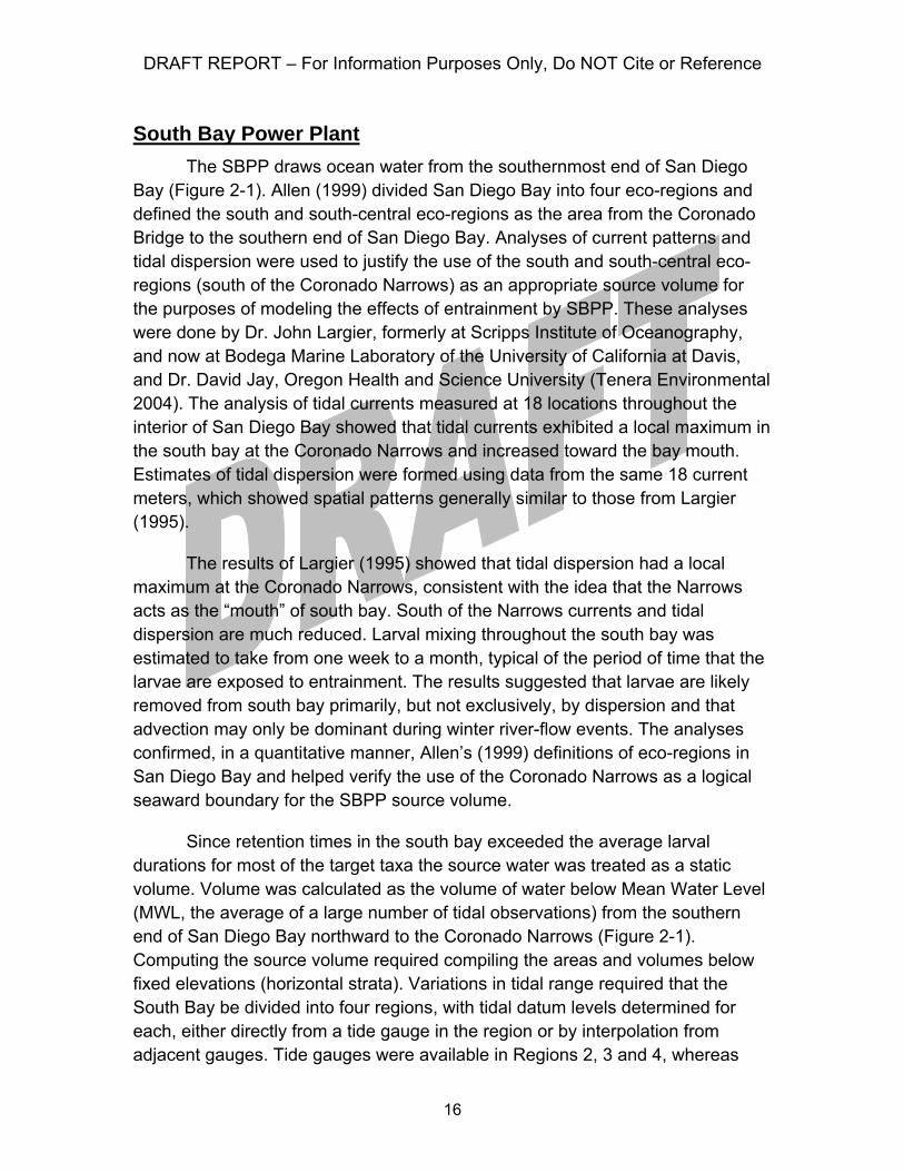
South Bay Power Plant The SBPP draws ocean water from the southernmost end of San Diego
Bay (Figure 2-1). Allen (1999) divided San Diego Bay into four eco-regions and defined the south and south-central eco-regions as the area from the Coronado Bridge to the southern end of San Diego Bay. Analyses of current patterns and tidal dispersion were used to justify the use of the south and south-central eco-regions (south of the Coronado Narrows) as an appropriate source volume for the purposes of modeling the effects of entrainment by SBPP. These analyses were done by Dr. John Largier, formerly at Scripps Institute of Oceanography, and now at Bodega Marine Laboratory of the University of California at Davis, and Dr. David Jay, Oregon Health and Science University (Tenera Environmental 2004). The analysis of tidal currents measured at 18 locations throughout the interior of San Diego Bay showed that tidal currents exhibited a local maximum in the south bay at the Coronado Narrows and increased toward the bay mouth. Estimates of tidal dispersion were formed using data from the same 18 current meters, which showed spatial patterns generally similar to those from Largier (1995).
The results of Largier (1995) showed that tidal dispersion had a local maximum at the Coronado Narrows, consistent with the idea that the Narrows acts as the “mouth” of south bay. South of the Narrows currents and tidal dispersion are much reduced. Larval mixing throughout the south bay was estimated to take from one week to a month, typical of the period of time that the larvae are exposed to entrainment. The results suggested that larvae are likely removed from south bay primarily, but not exclusively, by dispersion and that advection may only be dominant during winter river-flow events. The analyses confirmed, in a quantitative manner, Allen’s (1999) definitions of eco-regions in San Diego Bay and helped verify the use of the Coronado Narrows as a logical seaward boundary for the SBPP source volume.
Since retention times in the south bay exceeded the average larval durations for most of the target taxa the source water was treated as a static volume. Volume was calculated as the volume of water below Mean Water Level (MWL, the average of a large number of tidal observations) from the southern end of San Diego Bay northward to the Coronado Narrows (Figure 2-1). Computing the source volume required compiling the areas and volumes below fixed elevations (horizontal strata). Variations in tidal range required that the South Bay be divided into four regions, with tidal datum levels determined for each, either directly from a tide gauge in the region or by interpolation from adjacent gauges. Tide gauges were available in Regions 2, 3 and 4, whereas
DRAFT REPORT – For Information Purposes Only, Do NOT Cite or Reference
17
datum levels in Region 1 had to be determined by interpolation. Bathymetry for Regions 1 and 2 and the periphery of Regions 3 and 4 were obtained from the U.S. Navy and supplemented with data collected for this study. Estimates of the average concentrations of the organisms inside the bay were multiplied by the sum of the estimated volumes from the four areas (Table 2-2) to obtain estimates of the bay source water populations that were used in the calculations of mortality for the ETM.
Table 2-2. Source water body surface area and water volume at mean water level (MWL) by region for south San Diego Bay.
Region Datum Height (m) Area (m2) Volume (m3)
1 MWL 0.90 4,241,241 33,754,018 2 MWL 0.90 10,173,006 70,387,388 3 MWL 0.91 6,355,524 25,060,179 4 MWL 0.93 9,556,875 20,410,508
30,326,646 149,612,092
Morro Bay Power Plant The MBPP source water was divided into two sub-areas, bay water and
nearshore coastal water, because the location of the intake structure near the harbor entrance entrained both bay and nearshore species (Figure 2-2). The source water for MBPP could not be treated as a static volume, such as the source water for SBPP, because of the location of the power plant intake near the harbor entrance, which made it subject to tidal flows on a daily basis, and the smaller volume of the bay relative to an area such as San Diego Bay. To compensate for daily tidal movement past MBPP, the volume of the Morro Bay source water component was calculated as the sum of the bay’s twice daily exchange of its 15.5 million m3
tidal prism, adjusted for tidal exchange, (Mean High Water to Mean Low Water) and the bay’s non-tidal volume of 5.4 million m3. The volume of the tidal prism was adjusted to account for the portion of the Morro Bay outflow that returned with the incoming tide. Since volume was used to estimate the total supply of entrained larvae, inclusion of the re-circulated tidal prism volume would double count a portion of the larval supply and underestimate potential entrainment effects. This was accounted for using a tidal exchange ratio (TER), calculated for Morro Bay. The TER is the fraction of the total tidal exchange that consists of “new” water coming into the estuary, i.e., water that did not leave the estuary on the previous tidal cycle (Largier et al. 1996). In Morro Bay, the “total tidal exchange” is synonymous with the tidal prism, except for the amount estimated by TER.
DRAFT REPORT – For Information Purposes Only, Do NOT Cite or Reference
18
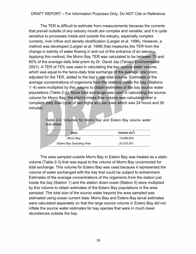
The TER is difficult to estimate from measurements because the currents that prevail outside of any estuary mouth are complex and variable, and it is quite sensitive to processes inside and outside the estuary, especially complex currents, river inflow and density stratification (Largier et al. 1996). However, a method was developed (Largier et al. 1996) that measures the TER from the change in salinity of water flowing in and out of the entrance of an estuary. Applying this method, the Morro Bay TER was calculated to be between 70 and 80% of the average daily tidal prism by Dr. David Jay (Tenera Environmental 2001). A TER of 75% was used in calculating the bay source water volume, which was equal to the twice-daily tidal exchange of the average tidal prism, adjusted for the TER, added to the bay’s non-tidal volume. Estimates of the average concentrations of organisms from the stations inside the bay (Stations 1−4) were multiplied by this volume to obtain estimates of the bay source water populations (Table 2-3). Since tidal exchange was used in calculating the source volume for Morro Bay, the plant’s intake flow volume was calculated over a complete daily tidal cycle of two highs and two lows which was 24 hours and 50 minutes.
Table 2-3. Volumes for Morro Bay and Estero Bay source water sub-areas.
Area Volume (m3)
Morro Bay 15,686,663
Estero Bay Sampling Area 20,915,551
The area sampled outside Morro Bay in Estero Bay was treated as a static volume (Table 2-3) that was equal to the volume of Morro Bay uncorrected for tidal exchange. This volume for Estero Bay was used because it represented the volume of water exchanged with the bay that could be subject to entrainment. Estimates of the average concentrations of the organisms from the station just inside the bay (Station 1) and the station down-coast (Station 5) were multiplied by this volume to obtain estimates of the Estero Bay populations in the area sampled. The total size of the source water beyond the area sampled was estimated using ocean current data. Morro Bay and Estero Bay larval estimates were calculated separately so that the large source volume in Estero Bay did not inflate the source water estimates for bay species that were in much lower abundances outside the bay.

DRAFT REPORT – For Information Purposes Only, Do NOT Cite or Reference
19
Diablo Canyon Power Plant The DCPP nearshore sampling was designed to only provide information
on abundance and distribution of target organisms in the vicinity of DCPP since it was recognized that the actual source water would be much larger for some species and also vary by species and seasonally due to changing oceanographic conditions. In establishing the nearshore sampling area, we considered that ocean currents in the area generally move both up and down the coast past DCPP. The currents also showed inshore/offshore oscillations, but these occurred less frequently and generally at a lower magnitude. The nearshore sampling area contained 64 stations or ‘cells’ (Figure 2-3) that was centered on the Intake Cove at DCPP. The northern extent of the sampling area was near Point Buchon and the southern half, a mirror image of the northern portion, extended to near Point San Luis. The shape of the sampling area reflected a slight bend (approximately 20º) in the coast at DCPP. The sampling area extended a distance of 8.7 km to both the north and south and an average distance of 3 km offshore. Regions inshore of the sampling area were in shallow water with partially submerged rocks, making the areas unsafe for boat operations and sampling. Volumes in each of the 64 cells were estimated using the surface area of the cell and the average depth based on available bathymetry data. The number of larvae in each cell was estimated by multiplying the average concentration during each survey by the volume of water sampled.
2.3 SAMPLING Sampling at all three of the facilities was designed to provide estimates of
both entrainment and source water concentrations that accounted for the differences in the cooling water volumes at the three plants and were representative of the range of habitats and organisms potentially affected by entrainment in each area. As a result of the differences among the three plants and funding available, the combined entrainment and source water sampling efforts ranged from five stations for the MBPP study to 68 stations for the DCPP study.
Sample collection methods were similar to those developed and used by CalCOFI in their larval fish studies (Smith and Richardson 1977). Sampling at all three plants was conducted using a bongo frame with two 71-cm diameter rings with plankton nets constructed of 333-um mesh. Each net was fitted with a Dacron sleeve and a cod-end container to retain the organisms. Each net was equipped with a calibrated General Oceanics flowmeter, which allowed the calculation of the amount of water filtered. Net lengths varied according to the
DRAFT REPORT – For Information Purposes Only, Do NOT Cite or Reference
20
depth of the water sampled. Shorter nets, 1.8 m in length, were used for entrainment sampling in the shallower intake cove at DCPP. Longer nets, 3.3 m in length were used for all other sampling. All of the nets were lowered as close to the bottom as possible and retrieved using oblique or vertical tows to sample the entire water column. Once the nets were retrieved from the water all of the collected material was rinsed into the codend. The target volume of each tow at both the entrainment and source water stations was 40-60 m3 for both nets combined. The sample volume was checked when the nets reached the surface and the tow continued or started over if the target volume was not collected. The contents of both nets were either combined into one sample immediately after collection, or treated as a single sample for analysis.
Entrainment sampling at all three plants was done in the waters outside of the plant CWIS as close as possible to the intake structure bar racks. This sampling design assumed that the concentrations from the waters in front of the CWIS are the same as the concentrations in the cooling water flow. Sampling was done outside of the CWIS because of the numerous problems involved in sampling inside the plant or at the discharge. Sampling inside the plant usually involves sampling with a pump that generally obtains a small volume relative to plankton nets in a given period of time. Although samples inside the CWIS may be well mixed, the cooling water flow inside the system is exposed to biofouling organisms that can significantly reduce the concentration of larval fish and other organisms. Sampling outside the plant also allowed entrainment samples to be used in characterizing source water populations. This was critical to the ETM calculations and allowed source water estimates to be calculated for species that may have only been collected from entrainment samples.
South Bay Power Plant Entrainment and source water sampling was conducted monthly from
January 2001 through January 2002 (Tenera Environmental 2004). Entrainment samples were collected from Station SB1 located in the SBPP intake channel (Figure 2-1). Each tow proceeded out the intake channel against the prevailing intake current. The intake channel was bounded by a separation dike to the south and a shallow mudflat to the north, and there was a constant current flow toward the intake structure. Therefore it was assumed that all of the water sampled at the entrainment station would be drawn through the SBPP cooling water system. Entrainment samples were collected over a 24-hour period, with each period divided into six 4-hour sampling cycles. Two replicate tows were collected consecutively at the entrainment station during each cycle. Source water samples at Stations SB2-SB9 were collected from the same vessel during
DRAFT REPORT – For Information Purposes Only, Do NOT Cite or Reference
21
the remainder of each cycle (Figure 2-1). A single tow was completed at each of the source water stations during each of the six 4-hr cycles.
The stations for the SBPP study (Figure 2-1) were stratified to include four channel locations on the east side of the bay and four shallower locations on the west side of the bay. The source water stations ranged in depth from approximately –2 m Mean Lower Low Water (MLLW) at SB8 to –12 m MLLW at SB9. This station array was chosen to include a range of depths and adjacent habitats in south San Diego Bay that would characterize the larval fish composition in the source water. For example, stations on the east side of the bay were adjacent to salt marsh habitat and would tend to have a greater proportion of larvae from species with demersal eggs that spawned in salt marsh channels, such as gobies, while deeper channel stations in the northern end of the study area would tend to have more larvae of species that spawn in open water such as northern anchovy (Engraulis mordax).
Morro Bay Power Plant Entrainment and source water sampling was conducted from December
1999 through December 2000 (Tenera Environmental 2001). Entrainment samples were collected weekly from in front of the MBPP intake structures (Station 2; Figure 2-2). Samples were collected over a continuous 24-hour period with each period divided into six, 4-hour sampling cycles. Two tows were conducted during each cycle. During the same period, monthly source water samples were collected at four stations in addition to the entrainment station (Figure 2-2). Initially, source water surveys were collected twice per day during daylight hours on high and low tides, but after two months of sampling in February 2000, sample collection for source water surveys was expanded to cover the entire 24-hour period and was no longer linked to tidal cycle.
Fewer stations were sampled in the MBPP study relative to the SBPP study due to the smaller size of the estuary. Station 1 was located just inside the entrance to Morro Bay and was intended to characterize water from outside the bay that was subject to entrainment during incoming tides. Only two other source water stations (stations 3 and 4) were located in Morro Bay because the areas that could be sampled in the south part of the bay were limited to narrow navigation channels. This was not considered to be a problem because of the large tidal prism relative to the size of the bay resulted in shallower portions of the bay draining through the deeper navigation channels where the sampling occurred. Station 5 was located outside of the bay approximately 4.7 km down
DRAFT REPORT – For Information Purposes Only, Do NOT Cite or Reference
22
coast (i.e., south of the harbor mouth) and was intended to characterize open coastal taxa potentially subject to entrainment.
Diablo Canyon Power Plant Collection of the DCPP entrainment samples occurred from October 1996
through June 1999 (Tenera Environmental 2000). This was the longest period of sampling among the three studies. The sampling was continued longer than one-year because of El Niño conditions during the first year, which were agreed by the Technical Workgroup as not representative of normal conditions. Entrainment samples were collected once per week from four permanently moored sampling stations located directly in front of the intake structure that were sampled in a random order during eight 3-hour cycles (Figure 2-3). Two samples were collected at each station during each cycle. The first 9 surveys were collected with 505 um mesh nets, but due to extrusion of larval fishes through the net mesh observed during these first few surveys, subsequent surveys were collected with 335 um mesh.
The boundaries and shape of the nearshore sampling area were chosen to ensure that the area would be large enough to characterize the larvae from the fishes potentially influenced by the large volume of the DCPP CWIS, and would be representative of the variety of nearshore habitats found in the area. These were the same reasons used to justify the large sampling effort (64 stations) relative to the SBPP and MBPP studies. Sampling of the nearshore study area occurred monthly from July 1997 through June 1999. Two randomly positioned stations within each of the 64 cells of the grid were sampled once each survey. The study grid was sampled continuously over 72 hours using a “ping-pong” transect to limit temporal and spatial biases in the sampling pattern and to optimize shipboard time. The starting cell (constrained to the 28 cells on the perimeter of the grid) and the initial direction of the transect (constrained to the two cells diagonally, adjacent to the starting cell) were selected at random. When the adjacent diagonal cell had previously been sampled, one of the two adjacent cells in the direction of travel was randomly selected to be sampled next. To minimize temporal variation between entrainment and study grid sampling, source water surveys were scheduled to bracket the 24-hour entrainment survey, overlapping by one day before and after the collection of entrainment samples.
Entrainment and nearshore sampling efforts did not start at the same times and therefore the entire sampling period was divided into five analysis periods. All of the weekly entrainment samples from October 1996 through November 1998 were processed so this period was divided into two yearlong
DRAFT REPORT – For Information Purposes Only, Do NOT Cite or Reference
23
analysis periods. Results for these periods are not presented because they were only used to generate estimates directly from entrainment data. The nearshore sampling period was also divided into two yearlong analysis periods. Only the entrainment samples collected during the sampling of the nearshore area were processed from December 1998 through June 1999 so entrainment data from July 1998 through June 1999 were used to generate model estimates for a fifth analysis period that could be directly compared with model estimates that incorporated data from the nearshore sampling area.
2.4 TARGET TAXA SELECTION Although almost all planktonic forms (phyto-, zoo-, and ichthyoplankton)
are affected by entrainment, these three studies and most other 316(b) studies have focused on a few target organism groups, typically ichthyoplankton and zooplankton. The effects on phytoplankton and invertebrate holoplankton are typically not studied because their large abundances, wide distributions, and short generation times should make them less susceptible to CWIS impacts. The target groups of organisms in these studies included larval fishes and larvae from commercially or recreationally important invertebrates such as Cancer spp. crabs and California spiny lobster (Panulirus interruptus).
Other potential target groups reviewed by the workgroups included kelp spores, fish eggs, squid paralarvae, and abalone and bivalve larvae. The risk of a significant impact on adult kelp populations by entrainment of kelp spores was determined to be negligible due to the large number of spores produced along the coast. Additionally, it is not possible to identify the species of kelp based on gametes or spores. Fish eggs were not included because they are difficult to identify to species and the most abundant fishes in these studies had egg stages that were not likely to be entrained; they either have demersal/adhesive eggs or are internally fertilized and extrude free-swimming larvae. Squid paralarvae are also unlikely to be entrained because they are competent swimmers immediately after hatching. Abalone larvae were not included because they are at low risk of entrainment and cannot be effectively sampled or identified during early life stages when they would be susceptible to entrainment (Tenera Environmental 1997). In addition, algal spores, fish eggs, and abalone and bivalve larvae would all require smaller mesh than the mesh used for ichthyoplankton and separate sampling efforts.
The final list of fish and invertebrates analyzed in each of the studies (Table 2-4) was determined by technical workgroups after all of the samples had been processed and data from the entrainment samples summarized. The

DRAFT REPORT – For Information Purposes Only, Do NOT Cite or Reference
24
Table 2-4. Target taxa used in assessments at South Bay (SBPP), Morro Bay (MBPP) and Diablo Canyon (DCPP) power plants.
Scientific Name Common Name
SBPP – species comprising 99 percent of total entrainment abundance Clevlandia ios, Ilypnus gilberti, Quietula y-cauda CIQ goby complex Gillichthys mirabilis longjaw mudsucker Anchoa spp. anchovies Atherinopsidae silversides Hypsoblennius spp. combtooth blennies MBPP – species comprising 90 percent of total entrainment abundance plus commercial species unidentified Gobiidae gobies Leptocottus armatus Pacific staghorn sculpin Stenobrachius leucopsarus northern lampfish Quietula y-cauda shadow goby Hypsoblennius spp. combtooth blennies Sebastes spp. V_De KGB rockfishes Atherinopsis californiensis jacksmelt Clupea pallasii Pacific herring Genyonemus lineatus white croaker Scorpaenichthys marmoratus cabezon Cancer antennarius brown rock crab Cancer jordani hairy rock crab Cancer anthonyi yellow crab Cancer gracilis slender crab Cancer productus red rock crab Cancer magister Dungeness crab DCPP – ten most abundant species plus commercial species Sardinops sagax Pacific sardine Engraulis mordax northern anchovy Sebastes spp. V / S. mystinus blue rockfish complex Sebastes spp. V_De/V_D_ KGB rockfish complex Oxylebius pictus painted greenling Artedius lateralis smoothhead sculpin Orthonopias triacis snubnose sculpin Scorpaenichthys marmoratus cabezon Genyonemus lineatus white croaker Cebidichthys violaceus monkeyface prickleback Gibbonsia spp. Clinid kelpfishes Rhinogobiops nicholsii blackeye goby Citharichthys spp. sanddabs Paralichthys californicus California halibut Cancer antennarius brown rock crab Cancer gracilis slender crab
DRAFT REPORT – For Information Purposes Only, Do NOT Cite or Reference
25
assessments included taxa from the target organism groups that were in highest abundance in the entrainment samples (generally those comprising up to 90% of the total abundance) and commercially or recreationally important fishes and invertebrates that were in high enough abundances to allow for their assessment. It was also realized that organisms having local adult and larval populations (i.e., source not sink species) were more important than species such as the northern lampfish (Stenobrachius leucopsarus), which is an offshore, deep-water species whose occurrence in entrainment was likely due to onshore currents that transported the larvae into coastal waters from their primary habitat. These ‘sink species’ were not included in the assessments.
The list of taxa reveals one of the problems with these studies. In some cases larvae cannot be identified to the species level and can only be identified into broader taxonomic groupings. Myomere and pigmentation patterns were used to identify many species, however this can be problematic for some species. For example, sympatric members of the family Gobiidae share morphologic and meristic characters during early life stages (Moser 1996) making identification to the species level difficult. In the MBPP study we grouped those gobiids we were unable to identify to species into an “unidentified gobiid” category (i.e., unidentified Gobiidae). In the SBPP study we were able to determine that the unidentified gobies were comprised of three species (Table 2-4). Larval combtooth blennies (Hypsoblennius spp.) can be easily distinguished from other larval fishes (Moser 1996). However, the three sympatric species along the central California coast cannot be distinguished from each other on the basis of morphometrics or meristics. These combtooth blennies were grouped into the “unidentified combtooth blennies” category (i.e., Hypsoblennius spp.). Many rockfish species (Sebastes spp.) are closely related, and the larvae share many morphological and meristic characteristics, making it difficult to visually identify them to species (Moser et al. 1977, Moser and Ahlstrom 1978, Baruskov 1981, Kendall and Lenarz 1987, Moreno 1993, Nishimoto in prep.). Identification of larval rockfish to the species level relies heavily on pigment patterns that change as the larvae develop (Moser 1996). Of the 59 rockfishes known from California marine waters (Lea et al. 1999), at least five can be reliably identified to the species level as larvae (Laidig et al. 1995, Yoklavich et al. 1996): blue rockfish (Sebastes mystinus), shortbelly rockfish (S. jordani), cowcod (S. levis), bocaccio (S. paucispinis), and stripetail rockfish (S. saxicola). The Sebastes larvae we collected could only be identified into broad sub-generic groupings based on pigment patterns; these larvae were grouped using information provided by Nishimoto (in prep.; Table 2-5). The use of these broad taxonomic categories presents problems in determining the most appropriate life history

DRAFT REPORT – For Information Purposes Only, Do NOT Cite or Reference
26
parameters to use in the demographic models. This involved calculating an average value or determining the most appropriate value from different sources and species.
Table 2-5. Pigment groups of some preflexion rockfish larvae from Nishimoto (in-prep).
The code for each group is based on the following letter designations: V_ = long series of ventral pigmentation (starts
directly at anus) De = elongating series of dorsal pigmentation
(scattered melanophores after continuous ones) V = short series of ventral pigmentation (starts 3-6
myomeres after anus) d = develops dorsal pigmentation (1-2 or scattered
melanophores) D_ = long series of dorsal pigmentation (4 or more in
a continuous line) extending to above anus P = pectoral blade pigmentation
D = short series of dorsal pigmentation (4 or more in a continuous line) not extending to anus
p = develops pectoral pigmentation (1-2 or scattered melanophores)
CODE SPECIES COMMON NAME
V D Long ventral series, short dorsal series, no pectoral pigment S. atrovirens kelp S. chrysomelas black and yellow S. maliger quillback S. nebulosus China S. semicinctus halfbanded
V_De Long ventral series, elongating dorsal series, pectoral pigmentOr S. auriculatus brown
V_DeP S. carnatus gopherOr S. caurinus copper
V_dep S. dalli calico S. rastrelliger grass
V Short ventral series, no dorsal series, no pectoral S. aleutianus rougheye S. alutus Pacific Ocean perch S. brevispinis silvergrey S. crameri darkblotched S. diploproa splitnose S. elongatus greenstriped S. macdonaldi Mexican S. miniatus vermilion S. nigrocinctus tiger S. proriger redstripe S. rosaceus rosy S. ruberrimus yelloweye S. serriceps treefish S. umbrosus honeycomb S. wilsoni pygmy S. zacentrus sharpchin
DRAFT REPORT – For Information Purposes Only, Do NOT Cite or Reference
27
2.5 OTHER BIOLOGICAL DATA All of the assessments models required some life history information from
a species to enable the calculation of entrainment effects. Age-specific survival and fecundity rates are required for the fecundity hindcasting (FH) and adult equivalent loss (AEL) demographic models. Calculation of FH requires egg and larval survivorship up to the age of entrainment plus estimates of lifetime fecundity, while AEL requires survivorship estimates from the age at entrainment to adult recruitment. Species-specific survivorship information (e.g., age-specific mortality) from egg or larvae to adulthood was not available for many of the taxa considered in the assessments at the three plants. Life history information was gathered from the scientific literature and other sources. Uncertainty surrounding published life history parameters is seldom known and rarely reported, but the likelihood that it is very large needs to be considered when interpreting results from the demographic approaches for estimating entrainment effects. Accuracy of the estimated entrainment effects from demographic models such as FH and AEL depend on the accuracy of age-specific mortality and fecundity estimates. In addition, these data are unavailable for many species limiting the application of these models to large numbers of species.
All three modeling approaches (FH, AEL, and ETM) required an age estimate of the entrained larvae. The larval ages were estimated using the length of the entrained larvae and an estimate of the larval growth rate for each species obtained from the scientific literature and other sources. The size range from the minimum to the average size of the larvae was used to calculate the average age of the entrained larvae that was used in the FH and AEL models, while the size range from the minimum to the maximum size of the larvae was used to calculate the maximum age of the entrained larvae and the period of time that the larvae were subject to entrainment for the ETM model. Minimum and maximum lengths used in these calculations were adjusted to account for potential outliers in the measurements by using the 1st and 99th percentile values in the calculations. The size range was estimated for each taxon from a representative sample of larvae from the SBPP and MBPP studies, while all of the entrained larvae of the target taxa were measured from the DCPP study. All of the measurements were made using a video capture system attached to a microscope and OptimasTM image analysis software.
2.6 PHYSICAL DATA COLLECTION Physical data were collected from sampling or other sources at all three
plants to estimate size of the source water and volume of the areas sampled. At
DRAFT REPORT – For Information Purposes Only, Do NOT Cite or Reference
28
SBPP and MBPP, hydrographic data collected for the study from several sources was used to estimate volume of the source water, which was equal to the sample volume for south San Diego Bay and Morro Bay. At DCPP, hydrographic data from National Oceanic and Atmospheric Administration was used to estimate the volumes of each of the 64-nearshore sampling stations. In addition, data on alongshore and onshore current velocities were measured using an InterOceans S4 current meter positioned approximately 1 km west of the DCPP intake at a depth of approximately 6 m (Figure 2-3). The direction in degrees true from north and speed in cm/s were estimated for each hour of the nearshore study grid survey periods. These data were used to estimate the size of the area that could have acted as a source for larvae in the nearshore sampling area (described below).
Data from the same current meter were used in the MBPP study to calculate an average current speed over the period of January 1, 1996 – May 31, 1999. Current direction was ignored in calculating the average speed. The current speed was used to estimate unidirectional displacement over the period of time that the larvae in the nearshore sampling area (Station 5) were exposed to entrainment (described below).
2.7 DATA REDUCTION
Entrainment Estimates Estimates of daily larval entrainment for all target organisms
(ichthyoplankton and selected invertebrate larvae) for all of the plants were calculated from data collected at the entrainment stations located directly in front of the power plant intake structures. Daily entrainment estimates were used to calculate daily incremental entrainment mortality estimates used in the ETM. Estimates of entrainment over annual study periods were used in the FH and AEL demographic modeling.
Daily entrainment estimates and their variances were derived from the mean concentration of larvae (number of larvae per cubic meter of water filtered) calculated from the samples collected during each 24-hr entrainment survey. These estimates were multiplied by the daily intake flow volume for each plant (MBPP and SBPP studies used engineering estimates of cooling water flow and DCPP used actual daily flow) to obtain the number of larvae entrained per day for each taxon as follows:

DRAFT REPORT – For Information Purposes Only, Do NOT Cite or Reference
29
ρ= ⋅i i iE v , (1)
where vi = total intake volume for the survey day of the ith survey period, and iρ = average concentration for the survey day of the ith survey period.
Entrainment was estimated for the days within each weekly (MBPP and DCPP) or monthly survey period (SBPP). The number of days in each period was determined by setting the sampling date at the mid-point between sample collections. Daily cooling water intake volumes were then used to calculate entrainment for the study period by summing the product of the entrainment estimates and the daily intake volumes for each survey period. These estimates and their associated variances were then added to obtain annual estimates of total entrainment and variance for each taxon as follows:
=
⎛ ⎞= ⎜ ⎟
⎝ ⎠∑
1
ni
T ii i
VE Ev
, (2)
where
=
=
=
intake volume on the survey day of the th survey period ( =1,...,n); total intake volume for the th survey period ( =1,...,n); and the estimate of daily entrainment during the entrainment
i
i
i
v i iV i iE survey of
the th survey period.i
with an associated variance of
=
⎛ ⎞= ⎜ ⎟
⎝ ⎠∑
2
1( ) ( )
ni
T ii i
VVar E Var Ev
, (3)
using the sampling variances of entrainment on the survey day of the ith period, Var(Ei). The daily sampling variance for SBPP and MBPP was calculated using the average concentrations from samples collected during each cycle, while the daily sampling variance for DCPP was calculated by treating each sampling cycle as a separate strata using data from the four entrainment stations. Both methods underestimated the true variance because they did not incorporate the variance associated with the within-survey period variation and daily variations in intake flow due to waves, tide, and other factors not measured by the power plant. One hundred percent mortality was assumed for all entrained organisms.
For the study at DCPP estimates of annual entrainment were scaled to better represent long-term trends for a taxa by using ichthyoplankton data collected inside the Intake Cove at DCPP (Figure 2-3). These data were used to calculate an index of annual trends in larval abundance for the period of 1990
DRAFT REPORT – For Information Purposes Only, Do NOT Cite or Reference
30
through 1998. This multi-year annualized index consisted of five months (February–June) of larval fish concentrations from 1990, six months (January–June) from 1991, and seven months (December–June) from all subsequent years. The estimated annual entrainment (ET) was adjusted to the long-term average using the following equation:
−
⎛ ⎞= ⋅⎜ ⎟
⎝ ⎠Adj T T
i
IE EI
, (4)
where
− = adjusted estimate of total annual entrainment to a long-term average, 1990 1998;
= index value from DCPP Intake Cove surface plankton tows for each th year; and
= average index value fro
Adj T
i
E
I i
I m DCPP Intake Cove surface plankton tows, 1990 1998.
Although the abundances used in calculating the index were not expected to be representative of the abundances calculated from the DCPP entrainment data, the use of the index does assume that the difference in abundance is approximately equal over time, although the validity of this assumption probably varied among taxa. Variance for adjusted annual entrainment can then be expressed as follows:
−
⎛ ⎞= ⋅⎜ ⎟
⎝ ⎠
2
( ) ( ),Adj T Ti
IVar E Var EI
(5)
assuming the indices are measured without error. Ignoring the sampling error of the indices will underestimate the true variance, but will qualitatively account for the change in scale associated with multiplying the annual entrainment estimate by a scalar. The variance of EAdj-T, however, does not take into account the between-day, within-station variance, interannual variation, nor the variance associated with the indices used in the adjustment. Hence, the actual variance of the EAdj-T estimate is likely to be greater than the value expressed above.
The Intake Cove surface tow index was assumed to have the following relationship:
= ⋅( )i iE I C E , (6)
where
DRAFT REPORT – For Information Purposes Only, Do NOT Cite or Reference
31
=
=
=
( ) expected value of the index for the th year; entrainment for the th year; and proportionality coefficient.
i
i
E I iE iC
If this relationship holds true and the differences over time are constant, then the inter-annual variance in the index has the following relationship:
= 2( ) ( ).i iVar I C Var E (7)
Therefore, the coefficients of variation (CV) for I and E across n years have the following relationship:
= =
2( ) ( )
( ) ( )
Var I C Var En nCV I CV EI CE
. (8)
Hence, the CV for the Intake Cove surface tow index should be a measure of the CV for entrainment across years. In the case of E and I, variances include sampling errors that may not be equal. Therefore, the CV of I was used to estimate variation in entrainment across years.
The use of adjusted entrainment in FH and AEL models at DCPP provided results that better represented average long-term effects. Adjusted entrainment values were not used in calculating ETM results because the computation of ETM relies on a proportional entrainment (PE) ratio using estimates from paired entrainment and nearshore larval sampling. Moreover, if the assumptions of the ETM model are valid, then the estimate already represents average long-term entrainment effects because the PE ratio should largely be a function of the ratio of the cooling water to source water volumes, which is constant compared to ichthyoplankton abundances that vary over time. This would especially be true if the PE were averaged over several taxa, assuming that the effects of larval behavior cancel across all the species. As a result the use of adjusted entrainment in FH and AEL models also provided a better basis to compare results from all three models when they were converted into a common currency through the use of population or fishery stock assessments.
2.8 SOURCE WATER ESTIMATES Average concentrations calculated from source water stations were used
to estimate source water populations of species or taxa groups using the same method used for calculating entrainment estimates for each ith survey period. At
DRAFT REPORT – For Information Purposes Only, Do NOT Cite or Reference
32
SBPP a single source water estimate was calculated, while at MBPP, separate estimates were calculated for Morro Bay and Estero Bay source water components.
At DCPP separate estimates were calculated for each of the 64 grid stations based on the depth and surface area of each station. In addition, an adjustment was made to the estimated number of larvae in the row 1 cells of the study grid to help compensate for the inability to safely collect samples inshore of the grid (Figure 2-3). The estimated volume of water directly inshore of the study grid was multiplied by the concentration of larvae collected in the row 1 cells, except for cells A1, D1, and E1. Cell A1 is more offshore than the rest of the cells in row 1 due to the bend in the coastline at Point Buchon and the adjustment was not done for the volume of water inshore of cell A1 because it would have added a substantial volume to that cell and the composition and abundance would not have been representative of the other inshore areas. Cells D1 and E1 are directly offshore from the Intake Cove where entrainment samples were collected. The average concentration from the entrainment stations was used for the areas inshore of cells D1 and E1. The estimated number of larvae in each grid station and from the areas inshore of the grid was added to obtain an estimate of the sampled source water populations.
2.9 IMPACT ASSESSMENT MODELS
Demographic Approaches Adult equivalent loss models (Goodyear 1978) evolved from impact
assessments that compared power plant losses to estimates of adult populations or commercial fisheries harvests. In the case of adult fishes impinged by intake screens, the comparison was relatively straightforward. To compare numbers of impinged sub-adults and juveniles and entrained larval fishes to adults, it was necessary to convert these losses to adult equivalents using demographic factors such as survival rates. Horst (1975) provided an early example of the equivalent adult model (EAM) to convert numbers of entrained early life stages of fishes to their hypothetical adult equivalency. Goodyear (1978) extended the method to include survival for several age classes of larvae.
Demographic approaches, exemplified by EAM, produce an absolute measure of loss beginning with simple numerical inventories of entrained or impinged individuals and increasing in complexity when the inventory results are extrapolated to estimate numbers of adult fishes or biomass. We used two different but related demographic approaches in assessing entrainment impacts

DRAFT REPORT – For Information Purposes Only, Do NOT Cite or Reference
33
at all three facilities: AEL (Goodyear 1978), which uses the larval losses to estimate the equivalent number of adult fishes that would not have been lost to the population and FH (Horst 1975, Goodyear 1978, MacCall, pers. comm.), which estimates the number of adult females at the age of maturity whose reproductive output has been lost due to entrainment. The method is similar to the Egg Production Method described by Parker (1980, 1985) and implemented in Parker and DeMartini (1989) at San Onofre Nuclear Generating Station except they used only eggs to hindcast adult equivalents.
Both AEL and FH approaches require an estimate of the age at entrainment for each taxon that was estimated by dividing the difference between the smallest (represented by the 1st percentile value) and the average lengths of a representative sample of larvae measured from the entrainment samples by a larval growth rate obtained from the literature. This assumes that the period of vulnerability to entrainment starts when the larvae are either hatched or released and that the smallest larvae in our samples represent newly hatched or released larvae. This minimum value was checked against reported hatch and release sizes for the taxa analyzed in these studies and in most cases was less than these reported values.
Additionally, age-specific survival and fecundity rates are required for calculating FH and AEL. FH requires egg and larval survivorship up to the age of entrainment plus estimates of fecundity, age at maturity and longevity, while AEL requires survivorship estimates from the age at entrainment to adult recruitment. Furthermore, to make estimation practical, the affected population is assumed to be stable and stationary, and age-specific survival and fecundity rates are assumed to be constant over time. In addition, the FH method assumes that all of the females instantaneously reach 100% maturity at the age of maturity.
Species-specific survivorship information from egg or larvae to adulthood was limited for many of the taxa considered in these studies. These rates when available were inferred from the literature along with estimates of uncertainty. Uncertainty surrounding published demographic parameters is seldom known and rarely reported, but the likelihood that it is very large needs to be considered when interpreting results from the demographic approaches for estimating entrainment effects. The ratio of the standard deviation to the mean (CV) was assumed to be 30% for all life history parameters used in the models for the SBPP and MBPP studies and 100% for the DCPP study. The larger CV was used at DCPP because it was the first study we conducted and we wanted to use a large CV to ensure that the confidence intervals adequately reflected the large degree of uncertainty associated with the estimates. The smaller CV used for
DRAFT REPORT – For Information Purposes Only, Do NOT Cite or Reference
34
SBPP and MBPP does not reflect increased confidence in the life history data, but our realization that the larger CV used at DCPP resulted in confidence intervals for the estimates that spanned several orders of magnitude minimizing their usefulness in the assessment.
Fecundity Hindcasting
The FH approach couples larval entrainment losses to adult fecundity using survivorship between stages to estimate the numbers of adult females at the age of maturity whose reproductive output has been lost due to entrainment, i.e., hindcasting the numbers of adult females at the age of maturity effectively removed from the reproductively active population. Accuracy of the estimate of impacts using this model is dependent upon an accurate estimate of survival from parturition through the estimated average age at entrainment and total lifetime female fecundity. If it can be assumed that the adult population has been stable at some current level of exploitation and that the male:female ratio is constant at 50:50, then fecundity and mortality are integrated into an estimate of adult loss at the age of female maturity by converting entrained larvae back into adult females and multiplying by two to approximate the total number of equivalent adults at the age of female maturity.
A potential advantage of FH is that survivorship need only be estimated for a relatively short period of the larval stage (e.g., egg to larval entrainment). The method requires age-specific mortality rates and fecundities to estimate equivalent adult losses. Furthermore, this method, as applied assumes a 50:50 male:female ratio, hence the loss of a single female’s reproductive potential was equivalent to the loss of two adult fish. Other assumptions included the following:
• Life history parameter values from the literature are representative of the population for the years and location of the study.
• Size of the stock does not affect survivorship or the rate of entrainment mortality.
• Reported values of egg mass were lifetime averages in order to calculate an unbiased estimate of lifetime fecundity.
• Total lifetime fecundity was accurately estimated by assuming that the mortality rate was uniform between age-at-maturity and longevity.
• ‘Knife-edge’ recruitment into the adult population at the age of maturity.
• Loss of the reproductive potential of one female was equivalent to the loss of an adult female at the age of maturity.
DRAFT REPORT – For Information Purposes Only, Do NOT Cite or Reference
35
The estimated number of females at the age of maturity whose lifetime reproductive potential was lost due to entrainment was calculated for each taxon as follows:
=
=
∏i1
Tn
jj
EFHTLF S
, (9)
where ET = total entrainment estimate;
Sj = survival rate from parturition to the average age of the entrained larvae at the end of the jth stage; and
TLF = average total lifetime fecundity (TLF) for females, equivalent to the average number of eggs spawned per female over their reproductive years.
While ET was used in the modeling at SBPP and MBPP, EAdj-T was used at DCPP. In practice, survival was estimated by either one or several age classes, depending on the data source, to the estimated age at entrainment. The expected TLF was approximated by the following expression:
= ⋅
⎛ ⎞= ⋅ ⎜ ⎟⎝ ⎠
Average eggs/year Average number of years of reproductive lifeLongevity - Age at maturationAverage eggs/year .
2
TLF
(10)
The number of years of reproductive potential was approximated as the midpoint between the ages of maturity and longevity. This approximation was based on the assumption of a linear uniform survivorship curve between these events (i.e., a uniform survival rate). Total lifetime fecundity for the studies at SBPP was calculated by adding 1 to the difference between longevity and age-at-maturity. This was done to account for spawning during the two ages used in the calculation. For heavily exploited species such as northern anchovy and sardine (Sardinops sagax), the expected number of years of reproductive potential may be much less than predicted using this assumption. Therefore, for the DCPP study the estimated longevity for heavily exploited fishes was based on the oldest observed individual caught by the fishery, rather than by the oldest recorded fish. If life table data are available for a taxon, then the lifetime fecundity should be estimated directly rather than using the approximation presented in Equation10. The variance of FH was approximated by the Delta method (Seber 1982) and is presented in Appendix A.
DRAFT REPORT – For Information Purposes Only, Do NOT Cite or Reference
36
Adult Equivalent Loss
The AEL approach uses abundance estimates of entrained or impinged organisms to project the loss of equivalent numbers of adults based on stage-specific survival and age-at-recruitment (Goodyear 1978). The primary advantage of this approach, and of FH, is that it translates power plant-induced early life-stage mortality into numbers of adult fishes, which are familiar units to resource managers. Adult equivalent loss does not require source water estimates of larval abundance in assessing effects. This latter advantage may be offset by the need to gather age-specific mortality rates to predict adult losses and the need for information on the adult population of interest for estimating population-level effects (i.e., fractional losses). Other assumptions of AEL using data on survivorship from entrainment to recruitment into the fishery assume the following:
• Published values of life history parameters are representative of the fish population in the years and location for the specific study.
• If survivorship values from the literature are limited to single observations, values are assumed constant over time or representative of the mean survivorship.
• No population reserve or compensation counters entrainment mortality.
• No compensatory mortality exists between entrainment mortality and natural mortality.
• Survival rates used in the calculations are representative and constant for the life stage of the larvae or fish in the calculations.
In some cases, survival rates estimated for a similar fish species were used. Should survivorship data from one species be substituted for another, then there is the following additional assumption:
• Values of survivorship for the two species are the same.
For fish species where larval survival data are missing, expected survival could be estimated using fecundity combined with juvenile and adult survival data. This approach requires the following additional assumption:
• The fish population is stationary in size such that each adult female contributes two new offspring to the population of adults during its lifetime.
Starting with the number of age class j larvae entrained, it is conceptually easy to convert the numbers to an equivalent number of adults lost at some specified age class using the following formula:

DRAFT REPORT – For Information Purposes Only, Do NOT Cite or Reference
37
=
= ∑1
n
j jj
AEL E S , (11)
where,
n = number of age classes;
Ej = estimated number of larvae lost per year in age class j; and
Sj = survival rate for the jth age class of the 1..n classes between entrainment and adulthood.
In practice, survival was estimated by either one or several age classes, depending on the data source, from the estimated age at entrainment to recruitment into the fishery. Survivorship to recruitment, at an adult age, was apportioned into several age stages, and AEL was calculated as follows:
=
= ∏1
n
T jj
AEL E S , (12)
where, th
jS = survival rate over the j age class.
The variance of AEL was approximated by the Delta method (Seber 1982) and is presented in Appendix A.
Alignment of FH and AEL Estimates
AEL and FH can be compared by assuming a stationary population where an adult female must produce two adults (i.e., one male and one female). These two adults are products of survival and total lifetime fecundity (TLF) modeled by the following expression:
= ⋅ ⋅ ⋅2 ,egg larvae adultS S S TLF (12)
which leads to the following:
=⋅ ⋅
2 .adultegg larvae
STLF S S
(13)
Substituting into the overall form of the following AEL equation:
= ⋅T adultAEL E S , (14)
DRAFT REPORT – For Information Purposes Only, Do NOT Cite or Reference
38
yields the following:
=⋅ ⋅2( )T
egg larva
EAELS S TLF
. (15)
Assuming a 50:50 sex ratio, without independent survival rates, AEL and FH are deterministically related as AEL≡2FH. The two estimates can be aligned so that female age at maturity is also the age of recruitment used in computing AEL. Otherwise, an alignment age can be accomplished by solving the simple exponential survival growth equation (Ricker 1975, Wilson and Bossert 1971):
− −= ⋅ 0( )0
Z t ttN N e , (16)
by substituting numbers of either equivalent adults or hindcast females, their associated ages, and mortality rates into the equation where,
=
=
==
0 0
number of adults at time ; number of adults at time ; instantaneous rate of natural mortality; and age of hindcast animals ( ) or extrapolated age of animals ( ).
tN tN tZt FH AEL
This allows for the alignment of ages for a population under equilibrium in either direction so they are either hindcast or extrapolated to the same age such that AEL≡2FH. Estimates of entrainment mortality calculated from AEL and FH approaches can be compared for similar time periods in taxa for which independent estimates are available for (1) survival from entrainment to the age at maturity, and (2) entrainment back to the number of eggs produced. This comparison serves as a method of cross-validating the two demographic models.
FH estimates the number of females at the age of maturity whose reproductive output is lost. The total number of females FN of all ages in the population can be estimated by the average fecundity as
=
=
∏1
TF n
jj
ENF Si
. (17)
AEL can be extrapolated to all mature female ages and summed to make a comparison to 2•NF using the preceding assumptions. The number of females whose reproductive output is lost in the population, NF, will be greater than the females estimated by FH. The analogue, sum of extrapolated AEL over adult
DRAFT REPORT – For Information Purposes Only, Do NOT Cite or Reference
39
ages, will be greater than AEL and represents the number of adult males and females lost.
Empirical Transport Model The ETM estimates conditional probability of mortality (PM) associated
with entrainment and requires an estimate of proportional entrainment (PE) as an input. Proportional entrainment is an estimate of the daily entrainment mortality on larval populations in the source water, independent of other sources of mortality. Following Ricker (1975), PE is an estimate of the conditional mortality rate. Proportional entrainment was calculated using the ratio of intake and source water abundances. In previous entrainment studies using the ETM method, intake concentrations were assumed from weighted population concentrations (Boreman et al. 1981). As proposed by the U.S. Fish and Wildlife Service (Boreman et al. 1978, 1981), ETM has been used to assess entrainment effects at the Salem Nuclear Generating Station in Delaware Bay, New Jersey and at other power stations along the east coast of the United States (Boreman et al. 1978, 1981; PSE&G 1993). Variations of this model have been discussed in MacCall et al. (1983) and used to assess impacts at the San Onofre Nuclear Generating Station (SONGS; Parker and DeMartini 1989).
The ETM estimates conditional mortality due to entrainment, while accounting for spatial and temporal variability in distribution and vulnerability of each life stage to cooling water withdrawals. The generalized form of the ETM incorporates many time-, space-, and age-specific estimates of mortality as well as information regarding spawning periodicity and larval duration (Boreman et al. 1978, 1981). Most of this information is limited or unknown for the taxa that were investigated for our studies. Thus, the applicability of ETM to these studies will be limited by the absence of empirically derived or reported demographic parameters needed as input to the model. Specifically, the length of time a larva is susceptible to entrainment must be estimated. However, by compounding the PE estimate over time, ETM can be used to estimate entrainment over a time period using assumptions about species-specific larval life histories, specifically the length of time in days that the larvae are in the water column and exposed to entrainment.
On any one sampling day i, the conditional entrainment mortality can be expressed as follows:

DRAFT REPORT – For Information Purposes Only, Do NOT Cite or Reference
40
= ii
i
EPEN
, (18)
where
Ei = total numbers of larvae entrained during a day during the ith survey;
and
Ni = numbers of larvae at risk of entrainment, i.e., abundance of larvae in
the sampled source water during a day during the ith survey.
Survival over one day = 1-PEi, and survival over the number of days (d) that the larvae are vulnerable to entrainment = (1-PEi)d, where d is estimated from the lengths of a representative sample of larvae collected over the entire study period. Values used in calculating PE are population estimates based on respective larval concentrations and volumes of the cooling water system flow and source water areas. The estimate of daily entrainment (Ei) was calculated using the methods described previously. The abundance of larvae at risk in the source water during the ith survey can be directly expressed as follows:
ρ= ⋅i S NiN V ,
(19)
where
VS = the static volume of the source water (N); and
ρiN = the average larval concentration in the source water during the ith
survey.
We note that the daily estimate of survival used by MacCall et al. (1983) and Boreman et al. (1981) is S=e-PE, which assumes the Baranov catch equation, E=FN, where F corresponds to PE and N is the average population size (Ricker 1975). Our estimate of daily survival assumes that N is the population size prior to entrainment. In our studies the outcome is approximately the same regardless of the type of survival estimates because PE values were weighted by large populations. When entrainment becomes relatively large it is recommended to use the Baranov-based estimate as in MacCall et al. (1983) because mortality estimates are reflective of average population size and also are larger.
At SBPP, and for taxa that were determined to primarily inhabit Morro Bay in the MBPP study, the estimated volumes of source water bodies previously

DRAFT REPORT – For Information Purposes Only, Do NOT Cite or Reference
41
described were used to estimate the abundance using an average concentration based on all of the samples from the source water for a given survey on a single day. At DCPP the equation to estimate PE for a day on which entrainment was sampled was:
= E
G
NPEN
, (20)
where =
×
estimated number of larvae entrained during the day, calculated as
(estimated concentration of larvae in the water entrained that day)
(design specified daily cooling water intake
EN
=
⋅∑64
i=1
volume); and
estimate of larvae in nearshore sampling area that day, calculated as
[(average concentration per cell) (cell volume)] for = 1, ..., 64 grid cells.
GN
i
where the estimated cell concentrations were obtained from the 72-hour source water survey that contained the 24-hour entrainment sampling period. In addition, an adjustment was made to the estimated number of larvae in the row 1 cells of the study grid to help compensate for the inability to safely collect samples inshore of the grid (Figure 2-3). The estimated volume of the water directly inshore of the study grid was multiplied by the concentration of larvae collected in the row 1 cells, except for cells A1, D1, and E1, as previously described.
Regardless of whether the species has a single spawning period per year or multiple overlapping spawnings the estimate of total larval entrainment mortality can be expressed as the following:
11 (1 )
nd
M i S ii
P f P PE=
= − −∑ , (21)
where = =
=
=
estimate of proportional entrainment for the th survey ( 1,...,n); proportion of sampled source water to total estimated source water; annual proportion of total larvae hatched during the
i
S
i
PE i iPf
=
th survey; and estimated number of days that the larvae are exposed to entrainment.
id
To establish independent survey estimates, it was assumed that each new survey represented a new, distinct cohort of larvae that was subject to entrainment. Each of the surveys was weighted using the proportion of the total population at risk during the ith survey (fi). In the original study plan and analyses
DRAFT REPORT – For Information Purposes Only, Do NOT Cite or Reference
42
for MBPP and DCPP studies we proposed to use the proportion of larvae entrained during each survey period as the weights for the ETM model. Weights were proposed to be calculated as follows:
= ii
T
EfE
, (22)
where Ei is estimated entrainment during the ith survey, and ET is estimated entrainment for the entire study period. This formulation conflicts with the formula for PE that uses the population in the source water during each survey to define the population at risk. If the weights are meant to represent the proportion of the population at risk during each survey then the weights should be calculated as follows:
= ii
T
NfN
, (23)
where Ni is the estimated fraction of the source population spawned during the ith survey, and NT is the total source population for the entire study period. Weights calculated using the entrainment estimates redefined the population at risk as the population entrained and represented a logical inconsistency in the model. Weights calculated using the source water estimates were used at SBPP and were used in final analyses of the data from the MBPP and DCPP studies in this paper.
The number of days that the larvae of a specific taxon were exposed to the mortality estimated by PE, was estimated using length data from a representative number of larvae from the entrainment samples. At SBPP, a single estimate of larval exposure was used in the calculations. The number of days (d) from hatching to entrainment was estimated by calculating the difference between the values of the 1st and upper 99th percentiles of the length measurements for each entrained larval taxon and dividing this range by an estimate of the larval growth rate for that taxon that was obtained from the scientific literature. The 1st and upper 99th percentiles were used to eliminate potential outlier measurements in the length data. In earlier studies at MBPP and DCPP, two estimates of d were calculated for each taxon and these were used to calculate two ETM estimates. The first estimate used an estimate of d calculated using the difference in length between the 1st and upper 99th percentiles and was used to represent the maximum number of days that the larvae were exposed to entrainment. The second estimate used an estimate of d calculated using the
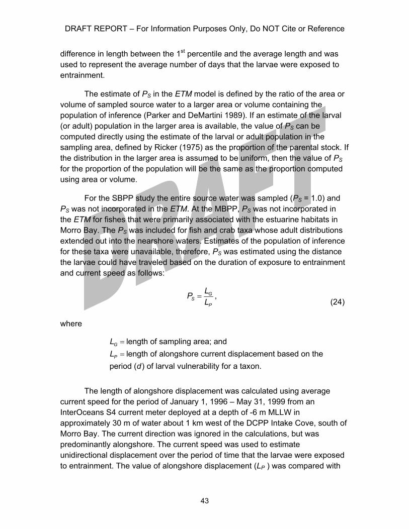
DRAFT REPORT – For Information Purposes Only, Do NOT Cite or Reference
43
difference in length between the 1st percentile and the average length and was used to represent the average number of days that the larvae were exposed to entrainment.
The estimate of PS in the ETM model is defined by the ratio of the area or volume of sampled source water to a larger area or volume containing the population of inference (Parker and DeMartini 1989). If an estimate of the larval (or adult) population in the larger area is available, the value of PS can be computed directly using the estimate of the larval or adult population in the sampling area, defined by Ricker (1975) as the proportion of the parental stock. If the distribution in the larger area is assumed to be uniform, then the value of PS for the proportion of the population will be the same as the proportion computed using area or volume.
For the SBPP study the entire source water was sampled (PS = 1.0) and PS was not incorporated in the ETM. At the MBPP, PS was not incorporated in the ETM for fishes that were primarily associated with the estuarine habitats in Morro Bay. The PS was included for fish and crab taxa whose adult distributions extended out into the nearshore waters. Estimates of the population of inference for these taxa were unavailable, therefore, PS was estimated using the distance the larvae could have traveled based on the duration of exposure to entrainment and current speed as follows:
= GS
P
LPL
, (24)
where
=
=
length of sampling area; andlength of alongshore current displacement based on the
period ( ) of larval vulnerability for a taxon.
G
P
LL
d
The length of alongshore displacement was calculated using average current speed for the period of January 1, 1996 – May 31, 1999 from an InterOceans S4 current meter deployed at a depth of -6 m MLLW in approximately 30 m of water about 1 km west of the DCPP Intake Cove, south of Morro Bay. The current direction was ignored in the calculations, but was predominantly alongshore. The current speed was used to estimate unidirectional displacement over the period of time that the larvae were exposed to entrainment. The value of alongshore displacement (LP ) was compared with
DRAFT REPORT – For Information Purposes Only, Do NOT Cite or Reference
44
the alongshore length of the sampled waterbody (LG). The distance between the west Morro Bay breakwater and Station 5 is 4.8 km; a value of 9.6 km (twice the distance) was used for LG. This value was used because it places Station 5 in the center of the sampled waterbody.
For the MBPP study we only presented a single estimate of PM for the taxa that used an adjustment for PS in the ETM, because any changes due to the increased duration were inversely proportional to the changes in PS, and resulted in nearly equal estimates of PM. (The exponential model [MacCall et al. 1983],
−1 sP PE te , gives equal estimates for PS inversely proportional to t). The estimate of the standard error is increased due to the extended period of entrainment risk, so two estimates of the standard error were presented for these taxa.
The sampling for the DCPP study was also extrapolated to provide an estimate of entrainment effects outside the nearshore sampling area. Boreman et al. (1981) point out that if any members of the population are located outside the sampled area, then the ETM will overestimate the conditional entrainment mortality for the entire population. In their study of entrainment at SONGS, Parker and DeMartini (1989) incorporated the inference population (which was an extrapolation to the entire Southern California Bight from the coast to a depth of 75 m, an area extending about 500 km) directly into their estimate of PE. In the DCPP ETM analyses, PE was multiplied by the estimated fraction of the population in the nearshore sampling area (Ps). The size of the population affected by entrainment varied from relatively small (e.g., the size of the sampling area) to very large (e.g., fishery management units, zoogeographic range). For some species an area approximately the size of the study grid represented the population of inference, and in these cases, PS≈1. For other species, the population of inference was larger than the study grid. The population of inference depended not only on the species, but also what appealed usefully to intuition, as a number of methods could be used for extrapolation. Therefore, the ETM was calculated over a range of values of PS for each of the target taxa. The resulting curves were used to determine the ETM at any value of PS. The curves were interpreted as a continuous probability function representing the risk of entrainment to the larvae at different values of PS. Point estimates of PM (and their ranges) were also calculated for each target taxon.
The relationship between PM and PS was represented by the sets of curves for each of the DCPP target taxa. Two point estimates of PS were also computed to account for the variation in the distribution of adult fishes included in the assessment. For offshore and subtidal target taxa whose larval distribution extends to the offshore edge of the study grid, SP was be calculated as follows:
DRAFT REPORT – For Information Purposes Only, Do NOT Cite or Reference
45
= GS
P
NPN
, (25)
where NG is the number of larvae in the study grid, and NP is the number of larvae in the population of inference. The numerator NG, presented earlier in the calculation of PE, was calculated as follows:
ρ=
= ⋅ ⋅∑64
i,k1
iG G kkk
N A D , (26)
where
kGA = area of grid cell k;
kD = average depth of the kth grid cell; and
ρ ik = concentration (per m3) of larvae in kth grid cell during survey i.
NP was estimated by an offshore and alongshore extrapolation of the study grid concentrations, using water current measurements. The following conceptual model was formulated to extrapolate larval concentrations (per m3) offshore of the grid:
ρ
ρ
=
=
⋅ ⋅ ⋅= =
⋅ ⋅ ⋅
∑
∑1
1
G
j
P
j
K
G j j jG i
S KP
P j j ji
L W DNPN L W D
, (27)
where
ρ
=
=
=
=
=
alongshore length of grid in the th stratum;
width of th stratum;alongshore length of population in th stratum based on current data;
average depth of th stratum; and average densit
j
j
G
j
P
j
j
L j
W jL j
D jy of larvae in th stratum.j
For this model, the grid was subdivided into KG alongshore strata (i.e., KG=8 rows in the grid) and the population into KG>KG alongshore strata. This approach described discrete values in intervals of a continuous function. Therefore, to ease implementation, an essentially equivalent formula used grid cell concentrations during the ith sampling period, ρ ,i k for a linear extrapolation of density (# per m2 calculated by multiplying ,i kρ by the cell depth) as a function of offshore distance, w :

DRAFT REPORT – For Information Purposes Only, Do NOT Cite or Reference
46
0
( )
i i
i Max
ii
i i
G GS W
PPG P
G W
N NP
LNN L w dw
Lρ
= =⎛ ⎞
+⎜ ⎟⎝ ⎠
∫,
(28)
where LP = alongshore length of population in the ith study period based on current displacement. The limits of integration are from the offshore margin of the study grid, WO, to a point estimated by the onshore movement of currents or where the density is zero or biologically limited, Wmax. Note that this point will usually occur outside the study grid area and that the population number, NP, is composed of two components that represent the alongshore extrapolation of the grid population and the offshore extrapolation of the alongshore grid population (Figure 2-3).
Alongshore and onshore current velocities used in the calculations were measured at a current meter positioned approximately 1 km west of the DCPP intake at a depth of approximately 6 m (Figure 2-3). The direction in degrees true from north and speed in cm/s were estimated for each hour of the nearshore study grid survey periods. Figure 2-4 shows the results of current meter analysis in which hourly current vectors were first rotated orthogonal to the coast by 49 degrees west of north. The movement of water was then tracked during the period from April 1997 through June 1999. A total alongshore length can be calculated from these data using the maximum up-coast and down-coast current movement over the larval duration period prior to each survey period. The maximum upcoast and downcoast current vectors measured during each survey period were added together to obtain an estimate of total alongshore displacement. Transport of larvae into the nearshore via onshore currents was also accounted for and used to set the limits of the offshore density extrapolation. Within this scenario, there were two subclasses:
1. For species in which the regression of density versus offshore distance had a negative slope, the offshore distance predicted where density was zero (i.e., integral of zero) was calculated. The alongshore distance was calculated from the water current data.
2. For species in which the regression of density versus offshore distance had a slope of >0, either the offshore distance from the water current data or an average distance based on the depth distribution of the adults offshore was used. Literature values (e.g., CalCOFI) were used to place a limit on both the distance and density values used in the offshore extrapolation.
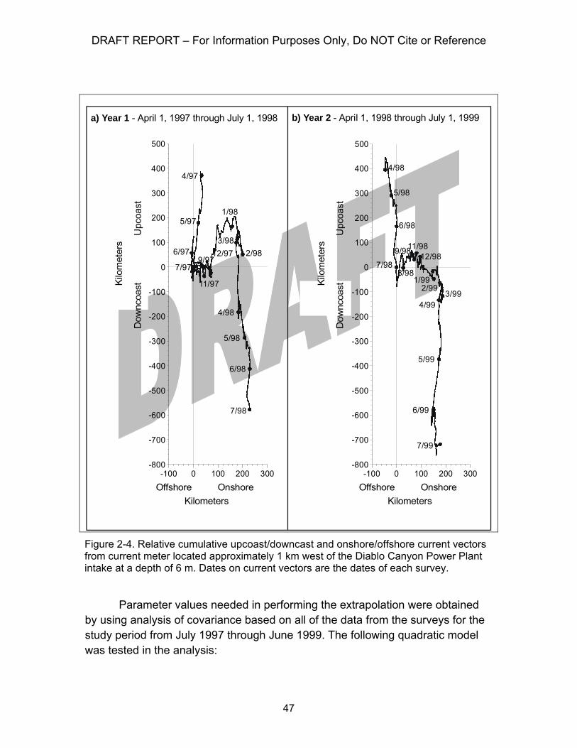
DRAFT REPORT – For Information Purposes Only, Do NOT Cite or Reference
47
Cumulative Current Movement
Kilometers Alongshore
-800
-700
-600
-500
-400
-300
-200
-100
0
100
200
300
400
500
Kilometers Onshore-100 0 100 200 300
4/97
5/97
6/97
7/97 9/97
11/97
12/97
1/98
2/98 3/98
4/98
5/98
6/98
7/98
Cumulative Current Movement
Kilometers Alongshore
-800
-700
-600
-500
-400
-300
-200
-100
0
100
200
300
400
500
Kilometers Onshore-100 0 100 200 300
4/98
5/98
6/98
7/988/98
9/98 11/98 12/98
1/99 2/99
3/99 4/99
5/99
6/99
7/99
Kilometers Kilometers Offshore Onshore Offshore Onshore
Dow
ncoa
st
U
pcoa
st
Dow
ncoa
st
U
pcoa
st
Kilo
met
ers
Kilo
met
ers
a) Year 1 - April 1, 1997 through July 1, 1998 b) Year 2 - April 1, 1998 through July 1, 1999
Figure 2-4. Relative cumulative upcoast/downcast and onshore/offshore current vectors from current meter located approximately 1 km west of the Diablo Canyon Power Plant intake at a depth of 6 m. Dates on current vectors are the dates of each survey.
Parameter values needed in performing the extrapolation were obtained by using analysis of covariance based on all of the data from the surveys for the study period from July 1997 through June 1999. The following quadratic model was tested in the analysis:

DRAFT REPORT – For Information Purposes Only, Do NOT Cite or Reference
48
2ij i ij if ijw wρ α β γ ε= + + + ,
(29)
where
ε
ρ
α β γ
=
=2
normally distributed error term with mean of zero; distance for the th observation in the th survey;
= larval density per m for the th observation in the th survey; and, , = regressi
i
ij
ij
w i j
i jon coefficients.
The following linear model produced a better fit in all cases:
ρ α β ε= + +ij i ij ijw . (30)
A common slope, β , for all surveys and unique intercepts, α i , for each survey were derived from the model. It is reasonable to assume a common slope, but differences in abundance between surveys required fitting different intercepts.
Variance calculations for PE are presented in Appendix A. Variance calculations for the estimate of PM are not presented because of the different approaches and parameters that will be used in the ETM calculations for each study.
DRAFT REPORT – For Information Purposes Only, Do NOT Cite or Reference
49
3.0 RESULTS
Detailed results for an example target taxon from each plant are presented to compare the modeling approaches for different source water body types. Results at SBPP are presented for the arrow, cheekspot, and shadow (Clevlandia ios, Ilypnus gilberti, and Quietula y-cauda [CIQ]) goby complex, which was the most abundant fish larvae collected during the study. At Morro Bay and Diablo Canyon, the kelp, gopher, and black-and-yellow (S. atrovirens, S. carnatus, and S. chrysomelas [KGB]) rockfish complex results provided illustrative data. These results provide example calculations for the FH and AEL models as well as for the ETM so that all three modeling approaches can be compared between sites.
The example taxa are indicative of the source water at the three study sites. Since SBPP used a fixed source water body volume the ETM model for all of the target taxa, including CIQ gobies, was calculated similarly. At MBPP, the ETM model for the target taxa that were designated as primarily inhabitants of Morro Bay was calculated using a fixed source water volume using calculations identical to those for CIQ gobies for the SBPP study. Therefore, we decided to present the ETM results for the KGB rockfish at MBPP since the source water for this taxon included both the bay and a nearshore area, the size of which was estimated using current meter data. A similar approach was taken for the DCPP study and, therefore, the results for the KGB rockfish complex are also presented for that study to provide a comparison with the results for MBPP.
3.1 SOUTH BAY POWER PLANT A total of 23,039 larval fishes in 20 taxonomic categories ranging from
ordinal to specific classifications was collected from 144 samples at the SBPP entrainment station (SB1) during monthly sampling from February 2001 through January 2002 (Table 3-1). These samples were used to estimate that total annual entrainment of fish larvae was 2.42 x 10⁹. Entrainment samples were dominated by gobies in the CIQ complex, which comprised about 76% of the total estimated entrainment. Five taxa evaluated for entrainment effects (Table 2-4) comprised greater than 99% of the total number of fish larvae entrained. No invertebrates were evaluated because only a single Cancer crab megalopae was collected.
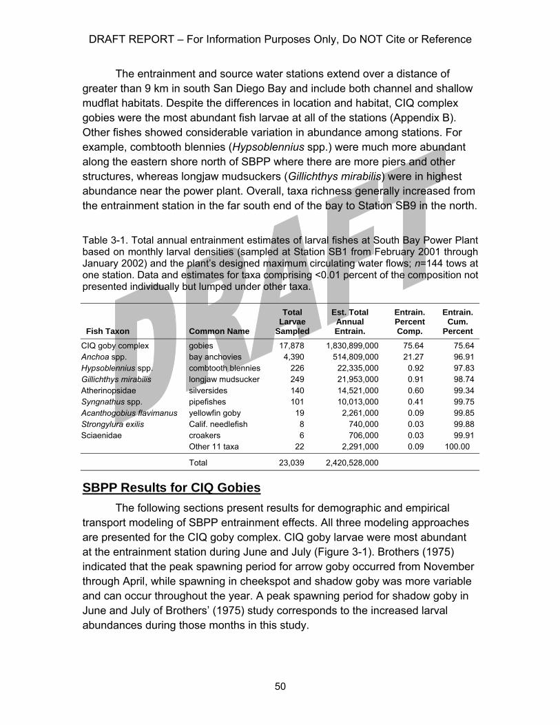
DRAFT REPORT – For Information Purposes Only, Do NOT Cite or Reference
50
The entrainment and source water stations extend over a distance of greater than 9 km in south San Diego Bay and include both channel and shallow mudflat habitats. Despite the differences in location and habitat, CIQ complex gobies were the most abundant fish larvae at all of the stations (Appendix B). Other fishes showed considerable variation in abundance among stations. For example, combtooth blennies (Hypsoblennius spp.) were much more abundant along the eastern shore north of SBPP where there are more piers and other structures, whereas longjaw mudsuckers (Gillichthys mirabilis) were in highest abundance near the power plant. Overall, taxa richness generally increased from the entrainment station in the far south end of the bay to Station SB9 in the north.
Table 3-1. Total annual entrainment estimates of larval fishes at South Bay Power Plant based on monthly larval densities (sampled at Station SB1 from February 2001 through January 2002) and the plant’s designed maximum circulating water flows; n=144 tows at one station. Data and estimates for taxa comprising <0.01 percent of the composition not presented individually but lumped under other taxa.
SBPP Results for CIQ Gobies The following sections present results for demographic and empirical
transport modeling of SBPP entrainment effects. All three modeling approaches are presented for the CIQ goby complex. CIQ goby larvae were most abundant at the entrainment station during June and July (Figure 3-1). Brothers (1975) indicated that the peak spawning period for arrow goby occurred from November through April, while spawning in cheekspot and shadow goby was more variable and can occur throughout the year. A peak spawning period for shadow goby in June and July of Brothers’ (1975) study corresponds to the increased larval abundances during those months in this study.
Fish Taxon Common Name
Total Larvae
Sampled
Est. Total Annual Entrain.
Entrain. Percent Comp.
Entrain.Cum.
Percent
CIQ goby complex gobies 17,878 1,830,899,000 75.64 75.64 Anchoa spp. bay anchovies 4,390 514,809,000 21.27 96.91 Hypsoblennius spp. combtooth blennies 226 22,335,000 0.92 97.83 Gillichthys mirabilis longjaw mudsucker 249 21,953,000 0.91 98.74 Atherinopsidae silversides 140 14,521,000 0.60 99.34 Syngnathus spp. pipefishes 101 10,013,000 0.41 99.75 Acanthogobius flavimanus yellowfin goby 19 2,261,000 0.09 99.85 Strongylura exilis Calif. needlefish 8 740,000 0.03 99.88 Sciaenidae croakers 6 706,000 0.03 99.91
Other 11 taxa 22 2,291,000 0.09 100.00
Total 23,039 2,420,528,000

DRAFT REPORT – For Information Purposes Only, Do NOT Cite or Reference
51
A) Entrainment Station
0
500
1000
1500
2000
2500
3000
3500
4000
4500
5000
5500
6000
Survey
01-Feb2001
01-Apr2001
01-Jun2001
01-Aug2001
01-Oct2001
01-Dec2001
01-Feb2002
Me
an
Co
nce
ntra
tion
(#/m
3 )
B) Source Water Stations
0
2000
4000
6000
8000
10000
12000
14000
16000
18000
20000
22000
24000
Survey
01-Feb2001
01-Apr2001
01-Jun2001
01-Aug2001
01-Oct2001
01-Dec2001
01-Feb2002
Mea
n C
onc
ent
ratio
n (#
/m3 )
Figure 3-1. Monthly mean larval concentration (standard error shown at top of dark bars) of the Clevlandia ios, Ilypnus gilberti, and Quietula y-cauda (CIQ) goby complex larvae at SBPP; A) intake entrainment station and B) source water stations.

DRAFT REPORT – For Information Purposes Only, Do NOT Cite or Reference
52
The ETM required an estimate of the length of time the larvae are susceptible to entrainment. The length frequency distribution for a representative sample of CIQ goby larvae showed that the majority of larvae were recently hatched based on the reported hatch size of 2–3 mm (Moser 1996) (Figure 3-2). The mean length of the collected CIQ goby larvae was 3.1 mm and the difference between the lengths of the 1st (2.2 mm) and 99th (5.8 mm) percentile values were used with a growth rate of 0.16 mm-d estimated from Brothers (1975) to determine that CIQ goby larvae were vulnerable to entrainment for a period of 22.9 days. The growth rate of 0.16 mm-d was determined using Brothers (1975) reported transformation lengths for the three species and an estimated transformation age of 60 d.
The comprehensive comparative study of the three goby species in the CIQ complex by Brothers (1975) also provided the necessary life history information for both FH and AEL demographic models and shows how life history data from the scientific literature are used in the modeling.
N = 390
Per
cent
0
10
20
30
40
50
Midpoint forLength Category (mm)
2.0 2.5 3.0 3.5 4.0 4.5 5.0 5.5 6.0 6.5 7.0 7.5 8.0 8.5 9.0 9.5 10.0 10.5 11.0
Figure 3-2. Length frequency distribution for Clevlandia ios, Ilypnus gilberti, and Quietula y-cauda (CIQ) goby complex larvae from the South Bay Power Plant entrainment station.
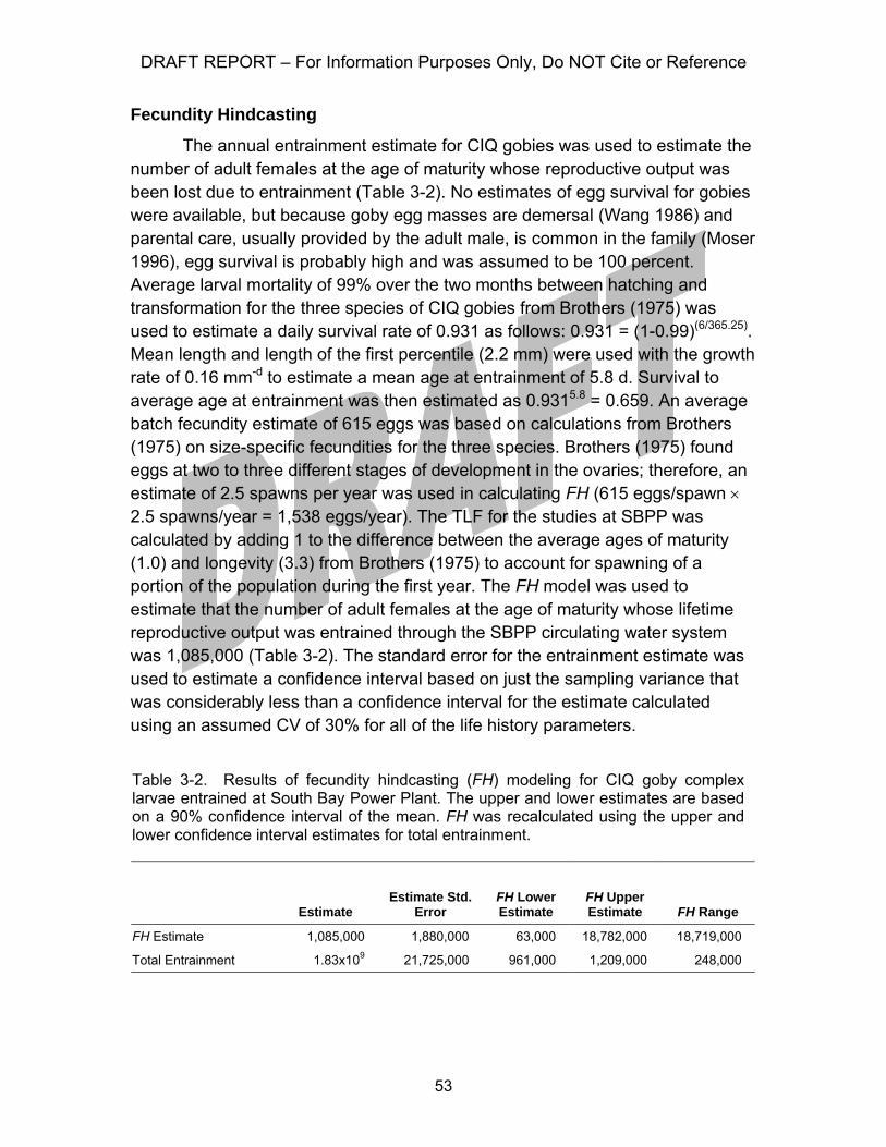
DRAFT REPORT – For Information Purposes Only, Do NOT Cite or Reference
53
Fecundity Hindcasting
The annual entrainment estimate for CIQ gobies was used to estimate the number of adult females at the age of maturity whose reproductive output was been lost due to entrainment (Table 3-2). No estimates of egg survival for gobies were available, but because goby egg masses are demersal (Wang 1986) and parental care, usually provided by the adult male, is common in the family (Moser 1996), egg survival is probably high and was assumed to be 100 percent. Average larval mortality of 99% over the two months between hatching and transformation for the three species of CIQ gobies from Brothers (1975) was used to estimate a daily survival rate of 0.931 as follows: 0.931 = (1-0.99)(6/365.25). Mean length and length of the first percentile (2.2 mm) were used with the growth rate of 0.16 mm-d to estimate a mean age at entrainment of 5.8 d. Survival to average age at entrainment was then estimated as 0.9315.8 = 0.659. An average batch fecundity estimate of 615 eggs was based on calculations from Brothers (1975) on size-specific fecundities for the three species. Brothers (1975) found eggs at two to three different stages of development in the ovaries; therefore, an estimate of 2.5 spawns per year was used in calculating FH (615 eggs/spawn × 2.5 spawns/year = 1,538 eggs/year). The TLF for the studies at SBPP was calculated by adding 1 to the difference between the average ages of maturity (1.0) and longevity (3.3) from Brothers (1975) to account for spawning of a portion of the population during the first year. The FH model was used to estimate that the number of adult females at the age of maturity whose lifetime reproductive output was entrained through the SBPP circulating water system was 1,085,000 (Table 3-2). The standard error for the entrainment estimate was used to estimate a confidence interval based on just the sampling variance that was considerably less than a confidence interval for the estimate calculated using an assumed CV of 30% for all of the life history parameters.
Table 3-2. Results of fecundity hindcasting (FH) modeling for CIQ goby complex larvae entrained at South Bay Power Plant. The upper and lower estimates are based on a 90% confidence interval of the mean. FH was recalculated using the upper and lower confidence interval estimates for total entrainment.
Estimate Estimate Std.
Error FH Lower Estimate
FH Upper Estimate FH Range
FH Estimate 1,085,000 1,880,000 63,000 18,782,000 18,719,000
Total Entrainment 1.83x10⁹ 21,725,000 961,000 1,209,000 248,000
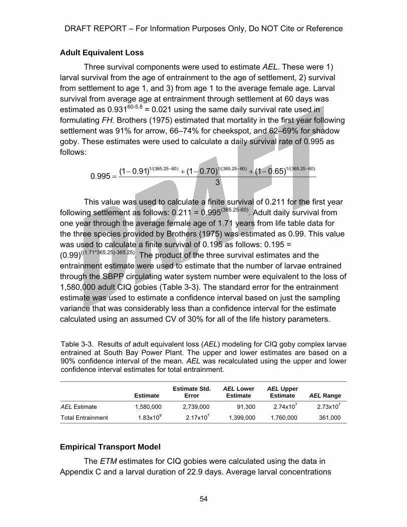
DRAFT REPORT – For Information Purposes Only, Do NOT Cite or Reference
54
Adult Equivalent Loss
Three survival components were used to estimate AEL. These were 1) larval survival from the age of entrainment to the age of settlement, 2) survival from settlement to age 1, and 3) from age 1 to the average female age. Larval survival from average age at entrainment through settlement at 60 days was estimated as 0.93160-5.8 = 0.021 using the same daily survival rate used in formulating FH. Brothers (1975) estimated that mortality in the first year following settlement was 91% for arrow, 66–74% for cheekspot, and 62–69% for shadow goby. These estimates were used to calculate a daily survival rate of 0.995 as follows:
− − −− + − + −
=1/(365.25 60) 1/(365.25 60) 1/(365.25 60)(1 0.91) (1 0.70) (1 0.65)0.995
3
This value was used to calculate a finite survival of 0.211 for the first year following settlement as follows: 0.211 = 0.995(365.25-60). Adult daily survival from one year through the average female age of 1.71 years from life table data for the three species provided by Brothers (1975) was estimated as 0.99. This value was used to calculate a finite survival of 0.195 as follows: 0.195 = (0.99)((1.71*365.25)-365.25). The product of the three survival estimates and the entrainment estimate were used to estimate that the number of larvae entrained through the SBPP circulating water system number were equivalent to the loss of 1,580,000 adult CIQ gobies (Table 3-3). The standard error for the entrainment estimate was used to estimate a confidence interval based on just the sampling variance that was considerably less than a confidence interval for the estimate calculated using an assumed CV of 30% for all of the life history parameters.
Table 3-3. Results of adult equivalent loss (AEL) modeling for CIQ goby complex larvae entrained at South Bay Power Plant. The upper and lower estimates are based on a 90% confidence interval of the mean. AEL was recalculated using the upper and lower confidence interval estimates for total entrainment.
Estimate Estimate Std.
Error AEL Lower Estimate
AEL Upper Estimate AEL Range
AEL Estimate 1,580,000 2,739,000 91,300 2.74x10⁷ 2.73x10⁷
Total Entrainment 1.83x10⁹ 2.17x10⁷ 1,399,000 1,760,000 361,000
Empirical Transport Model
The ETM estimates for CIQ gobies were calculated using the data in Appendix C and a larval duration of 22.9 days. Average larval concentrations
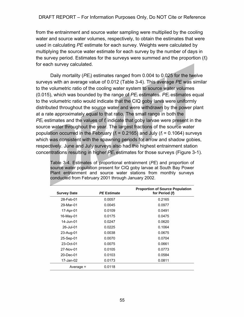
DRAFT REPORT – For Information Purposes Only, Do NOT Cite or Reference
55
from the entrainment and source water sampling were multiplied by the cooling water and source water volumes, respectively, to obtain the estimates that were used in calculating PE estimate for each survey. Weights were calculated by multiplying the source water estimate for each survey by the number of days in the survey period. Estimates for the surveys were summed and the proportion (fi) for each survey calculated.
Daily mortality (PEi) estimates ranged from 0.004 to 0.025 for the twelve surveys with an average value of 0.012 (Table 3-4). This average PE was similar to the volumetric ratio of the cooling water system to source water volumes (0.015), which was bounded by the range of PEi estimates. PEi estimates equal to the volumetric ratio would indicate that the CIQ goby larva were uniformly distributed throughout the source water and were withdrawn by the power plant at a rate approximately equal to that ratio. The small range in both the PEi estimates and the values of fi indicate that goby larvae were present in the source water throughout the year. The largest fractions of the source water population occurred in the February (fi = 0.2165) and July (fi = 0.1064) surveys which was consistent with the spawning periods for arrow and shadow gobies, respectively. June and July surveys also had the highest entrainment station concentrations resulting in higher PEi estimates for those surveys (Figure 3-1).
Table 3-4. Estimates of proportional entrainment (PE) and proportion of source water population present for CIQ goby larvae at South Bay Power Plant entrainment and source water stations from monthly surveys conducted from February 2001 through January 2002.
Survey Date PE Estimate
Proportion of Source Population for Period (f)
28-Feb-01 0.0057 0.2165 29-Mar-01 0.0045 0.0977 17-Apr-01 0.0109 0.0491
16-May-01 0.0175 0.0475 14-Jun-01 0.0247 0.0620 26-Jul-01 0.0225 0.1064
23-Aug-01 0.0038 0.0675 25-Sep-01 0.0070 0.0704 23-Oct-01 0.0075 0.0661 27-Nov-01 0.0105 0.0773 20-Dec-01 0.0103 0.0584 17-Jan-02 0.0173 0.0811
Average = 0.0118
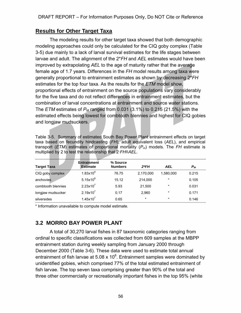
DRAFT REPORT – For Information Purposes Only, Do NOT Cite or Reference
56
Results for Other Target Taxa The modeling results for other target taxa showed that both demographic
modeling approaches could only be calculated for the CIQ goby complex (Table 3-5) due mainly to a lack of larval survival estimates for the life stages between larvae and adult. The alignment of the 2*FH and AEL estimates would have been improved by extrapolating AEL to the age of maturity rather that the average female age of 1.7 years. Differences in the FH model results among taxa were generally proportional to entrainment estimates as shown by decreasing 2*FH estimates for the top four taxa. As the results for the ETM model show, proportional effects of entrainment on the source populations vary considerably for the five taxa and do not reflect differences in entrainment estimates, but the combination of larval concentrations at entrainment and source water stations. The ETM estimates of PM ranged from 0.031 (3.1%) to 0.215 (21.5%) with the estimated effects being lowest for combtooth blennies and highest for CIQ gobies and longjaw mudsuckers.
3.2 MORRO BAY POWER PLANT A total of 30,270 larval fishes in 87 taxonomic categories ranging from
ordinal to specific classifications was collected from 609 samples at the MBPP entrainment station during weekly sampling from January 2000 through December 2000 (Table 3-6). These data were used to estimate total annual entrainment of fish larvae at 5.08 x 10⁸. Entrainment samples were dominated by unidentified gobies, which comprised 77% of the total estimated entrainment of fish larvae. The top seven taxa comprising greater than 90% of the total and three other commercially or recreationally important fishes in the top 95% (white
Table 3-5. Summary of estimated South Bay Power Plant entrainment effects on target taxa based on fecundity hindcasting (FH), adult equivalent loss (AEL), and empirical transport (ETM) estimates of proportional mortality (Pm) models. The FH estimate is multiplied by 2 to test the relationship that 2·FH≡AEL.
Target Taxa Entrainment
Estimate % Source Numbers 2*FH AEL PM
CIQ goby complex 1.83x10⁹ 76.75 2,170,000 1,580,000 0.215
anchovies 5.15x10⁸ 15.12 214,000 * 0.105
combtooth blennies 2.23x10⁷ 5.93 21,500 * 0.031
longjaw mudsucker 2.19x10⁷ 0.17 2,960 * 0.171
silversides 1.45x10⁷ 0.65 * * 0.146
* Information unavailable to compute model estimate.
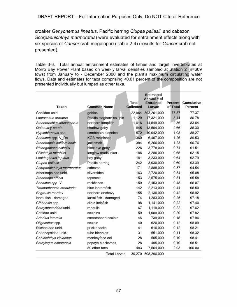
DRAFT REPORT – For Information Purposes Only, Do NOT Cite or Reference
57
croaker Genyonemus lineatus, Pacific herring Clupea pallasii, and cabezon Scorpaenichthys marmoratus) were evaluated for entrainment effects along with six species of Cancer crab megalopae (Table 2-4) (results for Cancer crab not presented).
Table 3-6. Total annual entrainment estimates of fishes and target invertebrates at Morro Bay Power Plant based on weekly larval densities sampled at Station 2 (n=609 tows) from January to - December 2000 and the plant’s maximum circulating water flows. Data and estimates for taxa comprising <0.01 percent of the composition are not presented individually but lumped as other taxa.
Taxon Common Name Total
Collected
Estimated Annual # of Entrained
Larvae Percent of Total
Cumulative Percent
Gobiidae unid. gobies 22,964 393,261,000 77.37 77.37 Leptocottus armatus Pacific staghorn sculpin 1,129 17,321,000 3.41 80.78 Stenobrachius leucopsarus northern lampfish 1,018 14,549,000 2.86 83.64 Quietula y-cauda shadow goby 845 13,504,000 2.66 86.30 Hypsoblennius spp. combtooth blennies 572 10,042,000 1.98 88.27 Sebastes spp. V_De KGB rockfishes 360 6,407,000 1.26 89.53 Atherinopsis californiensis jacksmelt 384 6,266,000 1.23 90.76 Rhinogobiops nicholsi blackeye goby 226 3,778,000 0.74 91.51 Gillichthys mirabilis longjaw mudsucker 186 3,286,000 0.65 92.15 Lepidogobius lepidus bay goby 181 3,233,000 0.64 92.79 Clupea pallasii Pacific herring 242 3,030,000 0.60 93.39 Scorpaenichthys marmoratus cabezon 171 2,888,000 0.57 94.54 Atherinopsidae unid. silversides 163 2,720,000 0.54 95.08 Atherinops affinis topsmelt 153 2,575,000 0.51 95.58 Sebastes spp. V rockfishes 150 2,453,000 0.48 96.07 Tarletonbeania crenularis blue lanternfish 142 2,213,000 0.44 96.50 Engraulis mordax northern anchovy 155 2,136,000 0.42 96.92 larval fish - damaged larval fish - damaged 74 1,283,000 0.25 97.18 Gibbonsia spp. clinid kelpfish 98 1,141,000 0.22 97.40 Bathymasteridae unid. ronquils 67 1,119,000 0.22 97.62 Cottidae unid. sculpins 59 1,009,000 0.20 97.82 Artedius lateralis smoothhead sculpin 46 739,000 0.15 97.96 Oligocottus spp. sculpin 40 620,000 0.12 98.09 Stichaeidae unid. pricklebacks 41 616,000 0.12 98.21 Chaenopsidae unid. tube blennies 31 551,000 0.11 98.32 Cebidichthys violaceus monkeyface eel 28 505,000 0.10 98.41 Bathylagus ochotensis popeye blacksmelt 28 495,000 0.10 98.51
59 other taxa 483 7,564,000 2.93 100.00
Total Larvae 30,270 508,296,000

DRAFT REPORT – For Information Purposes Only, Do NOT Cite or Reference
58
Species composition for entrainment at MBPP was much more diverse than the results from SBPP. This may have resulted from the more frequent weekly sampling at MBPP and the location of the power plant near the entrance to the bay relative to the back bay location of SBPP. Entrainment was dominated by fishes that primarily occur as adults in the bay, such as gobies, but also included numerous fishes that are more typically associated with nearshore coastal habitats, such as rockfish and cabezon.
MBPP Results for the KGB Rockfish Complex Detailed results and details on the data used in the three modeling
approaches at MBPP are presented for the KGB larval rockfish complex. KGB rockfish had the sixth highest estimated entrainment (6,407,000) or 1.3% of the total larval fishes (Table 3-6). Consistent with the annual spawning period for most rockfishes (Parrish et al. 1989), larvae occurred in entrainment samples from January through June with the highest abundances in April (Figure 3-3). Results from source water surveys showed the same abundance peaks seen in samples collected at the MBPP intake station (Figure 3-4). Although not collected every month, KGB rockfish larvae were collected from all of the stations inside Morro Bay during the April survey. They reached their greatest concentration at the Estero Bay Station 5 during the May survey when they were less common at the stations inside Morro Bay.
The length frequency distribution for a representative sample of KGB rockfish larvae showed a relatively narrow size range of 3.4 to 5.4 mm (1st and 99th percentile values = 3.5 and 5.1) with an average size of 4.3 mm (Figure 3-5). These results indicate that most of the larvae are less than the maximum reported size at extrusion of 4.0–5.5 mm (Moser 1996) and are therefore subject to entrainment for a relatively short period of time. There are no studies on the larval growth rates for the species in the KGB rockfish complex so a larval growth rate of 0.14 mm-d from brown rockfish (Love and Johnson 1999, Yoklavich et al. 1996) was used in estimating that the average age at entrainment was 5.5 d and the maximum age at entrainment, based on the 99th percentile values was 11.3 d.
Fecundity Hindcast Model
Total annual larval entrainment for KGB rockfish was used to estimate the number of adult females at the age of maturity whose reproductive output was been lost due to entrainment (Table 3-7). The parameters required for formulation of FH estimates for KGB rockfishes were compiled from references
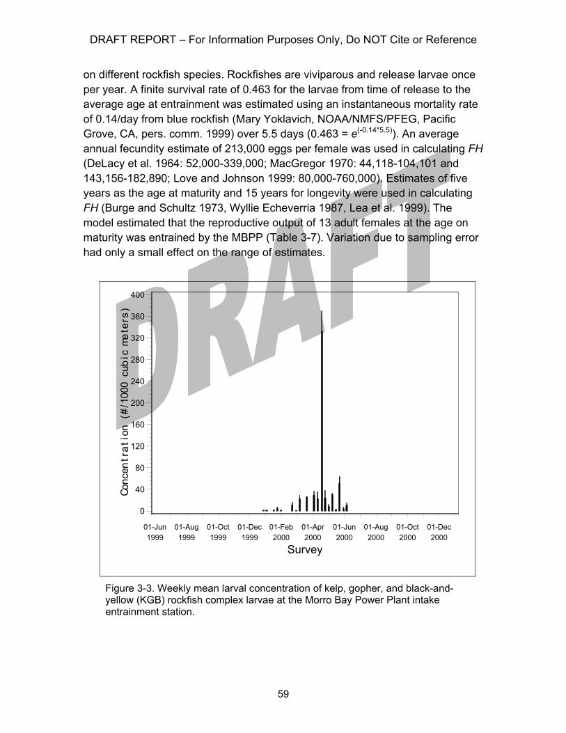
DRAFT REPORT – For Information Purposes Only, Do NOT Cite or Reference
59
on different rockfish species. Rockfishes are viviparous and release larvae once per year. A finite survival rate of 0.463 for the larvae from time of release to the average age at entrainment was estimated using an instantaneous mortality rate of 0.14/day from blue rockfish (Mary Yoklavich, NOAA/NMFS/PFEG, Pacific Grove, CA, pers. comm. 1999) over 5.5 days (0.463 = e(-0.14*5.5)). An average annual fecundity estimate of 213,000 eggs per female was used in calculating FH (DeLacy et al. 1964: 52,000-339,000; MacGregor 1970: 44,118-104,101 and 143,156-182,890; Love and Johnson 1999: 80,000-760,000). Estimates of five years as the age at maturity and 15 years for longevity were used in calculating FH (Burge and Schultz 1973, Wyllie Echeverria 1987, Lea et al. 1999). The model estimated that the reproductive output of 13 adult females at the age on maturity was entrained by the MBPP (Table 3-7). Variation due to sampling error had only a small effect on the range of estimates.
Figure 3-3. Weekly mean larval concentration of kelp, gopher, and black-and-yellow (KGB) rockfish complex larvae at the Morro Bay Power Plant intake entrainment station.
Conc
entr
atio
n (#
/100
0 cu
bic
met
ers)
0
40
80
120
160
200
240
280
320
360
400
Survey
01-Jun1999
01-Aug1999
01-Oct1999
01-Dec1999
01-Feb2000
01-Apr2000
01-Jun2000
01-Aug2000
01-Oct2000
01-Dec2000
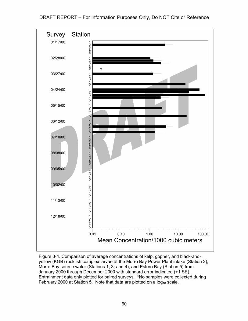
DRAFT REPORT – For Information Purposes Only, Do NOT Cite or Reference
60
Figure 3-4. Comparison of average concentrations of kelp, gopher, and black-and-yellow (KGB) rockfish complex larvae at the Morro Bay Power Plant intake (Station 2), Morro Bay source water (Stations 1, 3, and 4), and Estero Bay (Station 5) from January 2000 through December 2000 with standard error indicated (+1 SE). Entrainment data only plotted for paired surveys. *No samples were collected during February 2000 at Station 5. Note that data are plotted on a log10 scale.
StationSurvey
12/18/00
11/13/00
10/02/00
09/05/00
08/08/00
07/10/00
06/12/00
05/15/00
04/24/00
03/27/00
02/28/00
01/17/00
54321
54321
54321
54321
54321
54321
54321
54321
54321
54321
54321
54321
Mean Concentration/1000 cubic meters0.01 0.10 1.00 10.00 100.00
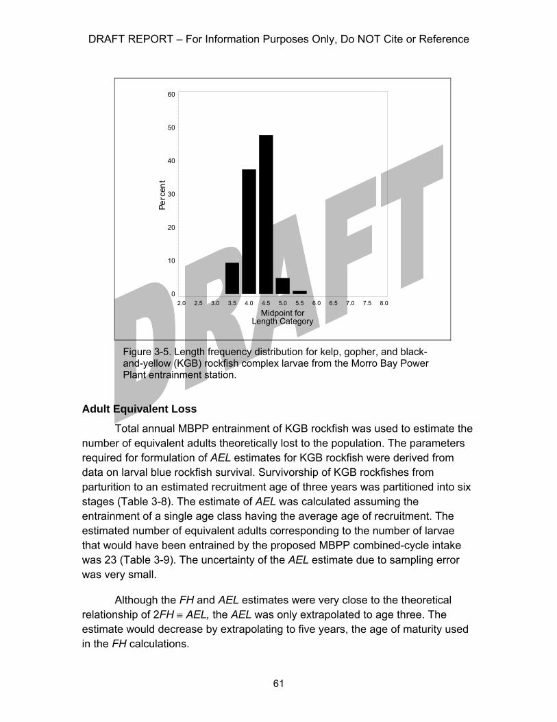
DRAFT REPORT – For Information Purposes Only, Do NOT Cite or Reference
61
Figure 3-5. Length frequency distribution for kelp, gopher, and black-and-yellow (KGB) rockfish complex larvae from the Morro Bay Power Plant entrainment station.
Adult Equivalent Loss
Total annual MBPP entrainment of KGB rockfish was used to estimate the number of equivalent adults theoretically lost to the population. The parameters required for formulation of AEL estimates for KGB rockfish were derived from data on larval blue rockfish survival. Survivorship of KGB rockfishes from parturition to an estimated recruitment age of three years was partitioned into six stages (Table 3-8). The estimate of AEL was calculated assuming the entrainment of a single age class having the average age of recruitment. The estimated number of equivalent adults corresponding to the number of larvae that would have been entrained by the proposed MBPP combined-cycle intake was 23 (Table 3-9). The uncertainty of the AEL estimate due to sampling error was very small.
Although the FH and AEL estimates were very close to the theoretical relationship of 2FH ≡ AEL, the AEL was only extrapolated to age three. The estimate would decrease by extrapolating to five years, the age of maturity used in the FH calculations.
Perc
ent
0
10
20
30
40
50
60
Midpoint forLength Category
2.0 2.5 3.0 3.5 4.0 4.5 5.0 5.5 6.0 6.5 7.0 7.5 8.0
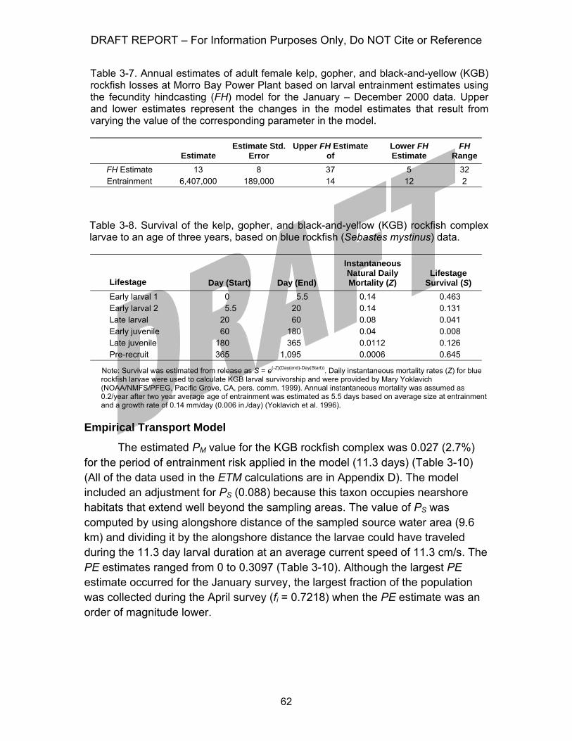
DRAFT REPORT – For Information Purposes Only, Do NOT Cite or Reference
62
Table 3-7. Annual estimates of adult female kelp, gopher, and black-and-yellow (KGB) rockfish losses at Morro Bay Power Plant based on larval entrainment estimates using the fecundity hindcasting (FH) model for the January – December 2000 data. Upper and lower estimates represent the changes in the model estimates that result from varying the value of the corresponding parameter in the model.
Estimate Estimate Std.
Error Upper FH Estimate
of Lower FH Estimate
FH Range
FH Estimate 13 8 37 5 32 Entrainment 6,407,000 189,000 14 12 2
Table 3-8. Survival of the kelp, gopher, and black-and-yellow (KGB) rockfish complex larvae to an age of three years, based on blue rockfish (Sebastes mystinus) data.
Lifestage Day (Start) Day (End)
Instantaneous Natural Daily Mortality (Z)
Lifestage Survival (S)
Early larval 1 0 5.5 0.14 0.463 Early larval 2 5.5 20 0.14 0.131 Late larval 20 60 0.08 0.041 Early juvenile 60 180 0.04 0.008 Late juvenile 180 365 0.0112 0.126 Pre-recruit 365 1,095 0.0006 0.645
Note: Survival was estimated from release as S = e(-Z)(Day(end)-Day(Start)). Daily instantaneous mortality rates (Z) for blue rockfish larvae were used to calculate KGB larval survivorship and were provided by Mary Yoklavich (NOAA/NMFS/PFEG, Pacific Grove, CA, pers. comm. 1999). Annual instantaneous mortality was assumed as 0.2/year after two year average age of entrainment was estimated as 5.5 days based on average size at entrainment and a growth rate of 0.14 mm/day (0.006 in./day) (Yoklavich et al. 1996).
Empirical Transport Model
The estimated PM value for the KGB rockfish complex was 0.027 (2.7%) for the period of entrainment risk applied in the model (11.3 days) (Table 3-10) (All of the data used in the ETM calculations are in Appendix D). The model included an adjustment for PS (0.088) because this taxon occupies nearshore habitats that extend well beyond the sampling areas. The value of PS was computed by using alongshore distance of the sampled source water area (9.6 km) and dividing it by the alongshore distance the larvae could have traveled during the 11.3 day larval duration at an average current speed of 11.3 cm/s. The PE estimates ranged from 0 to 0.3097 (Table 3-10). Although the largest PE estimate occurred for the January survey, the largest fraction of the population was collected during the April survey (fi = 0.7218) when the PE estimate was an order of magnitude lower.
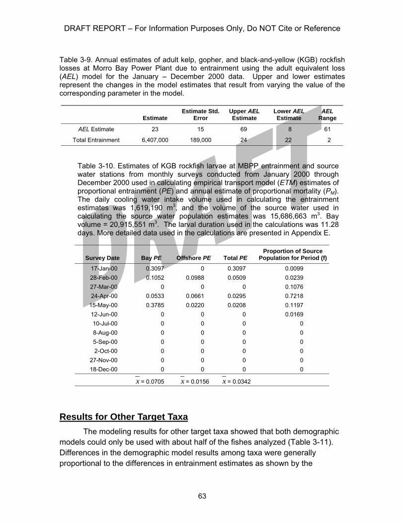
DRAFT REPORT – For Information Purposes Only, Do NOT Cite or Reference
63
Table 3-9. Annual estimates of adult kelp, gopher, and black-and-yellow (KGB) rockfish losses at Morro Bay Power Plant due to entrainment using the adult equivalent loss (AEL) model for the January – December 2000 data. Upper and lower estimates represent the changes in the model estimates that result from varying the value of the corresponding parameter in the model.
Estimate Estimate Std.
Error Upper AEL Estimate
Lower AEL Estimate
AEL Range
AEL Estimate 23 15 69 8 61
Total Entrainment 6,407,000 189,000 24 22 2
Table 3-10. Estimates of KGB rockfish larvae at MBPP entrainment and source water stations from monthly surveys conducted from January 2000 through December 2000 used in calculating empirical transport model (ETM) estimates of proportional entrainment (PE) and annual estimate of proportional mortality (PM). The daily cooling water intake volume used in calculating the entrainment estimates was 1,619,190 m3, and the volume of the source water used in calculating the source water population estimates was 15,686,663 m3. Bay volume = 20,915,551 m3. The larval duration used in the calculations was 11.28 days. More detailed data used in the calculations are presented in Appendix E.
Survey Date Bay PE Offshore PE Total PE Proportion of Source
Population for Period (f)
17-Jan-00 0.3097 0 0.3097 0.0099 28-Feb-00 0.1052 0.0988 0.0509 0.0239 27-Mar-00 0 0 0 0.1076 24-Apr-00 0.0533 0.0661 0.0295 0.7218
15-May-00 0.3785 0.0220 0.0208 0.1197 12-Jun-00 0 0 0 0.0169 10-Jul-00 0 0 0 0 8-Aug-00 0 0 0 0 5-Sep-00 0 0 0 0 2-Oct-00 0 0 0 0
27-Nov-00 0 0 0 0 18-Dec-00 0 0 0 0
x = 0.0705 x = 0.0156 x = 0.0342
Results for Other Target Taxa The modeling results for other target taxa showed that both demographic
models could only be used with about half of the fishes analyzed (Table 3-11). Differences in the demographic model results among taxa were generally proportional to the differences in entrainment estimates as shown by the
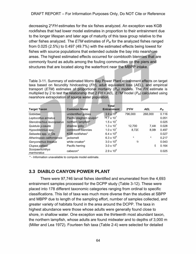
DRAFT REPORT – For Information Purposes Only, Do NOT Cite or Reference
64
decreasing 2*FH estimates for the six fishes analyzed. An exception was KGB rockfishes that had lower model estimates in proportion to their entrainment due to the longer lifespan and later age of maturity of this taxa group relative to the other fishes analyzed. The ETM estimates of PM for the analyzed fishes ranged from 0.025 (2.5%) to 0.497 (49.7%) with the estimated effects being lowest for fishes with source populations that extended outside the bay into nearshore areas. The highest estimated effects occurred for combtooth blennies that are commonly found as adults among the fouling communities on the piers and structures that are located along the waterfront near the MBPP intake.
Table 3-11. Summary of estimated Morro Bay Power Plant entrainment effects on target taxa based on fecundity hindcasting (FH), adult equivalent loss (AEL), and empirical transport (ETM) estimates of proportional mortality (PM) models. The FH estimate is multiplied by 2 to test the relationship that 2·FH = AEL. ETM model (PM) calculated using nearshore extrapolation of source water population.
Target Taxon Common Name Total
Entrainment 2*FH AEL PM Gobiidae unidentified gobies 3.9 x 10⁸ 796,000 268,000 0.116Leptocottus armatus Pacific staghorn sculpin* 1.7 x 10⁷ 0.051Stenobrachius leucopsarus northern lampfish* 1.5 x 10⁷ 0.025Quietula y-cauda shadow goby 1.3 x 10⁷ 12,700 7,440 0.028Hypsoblennius spp. combtooth blennies 1.0 x 10⁷ 8,720 8,080 0.497Sebastes spp. V_De KGB rockfishes* 6.4 x 10⁶ 0.027Atherinopsis californiensis jacksmelt 6.3 x 10⁶ * * 0.217Genyonemus lineatus white croaker* 3.0 x 10⁶ 10 0.043Clupea pallasii Pacific herring 3.0 x 10⁶ 5 0.164Scorpaenichthys marmoratus cabezon* 2.9 x 10⁶ 0.025
* - Information unavailable to compute model estimate.
3.3 DIABLO CANYON POWER PLANT There were 97,746 larval fishes identified and enumerated from the 4,693
entrainment samples processed for the DCPP study (Table 3-12). These were placed into 178 different taxonomic categories ranging from ordinal to specific classifications. This list of taxa was much more diverse than the studies at SBPP and MBPP due to length of the sampling effort, number of samples collected, and greater variety of habitats found in the area around the DCPP. The taxa in highest abundance were those whose adults were generally found close to shore, in shallow water. One exception was the thirteenth most abundant taxon, the northern lampfish, whose adults are found midwater and to depths of 3,000 m (Miller and Lea 1972). Fourteen fish taxa (Table 2-4) were selected for detailed
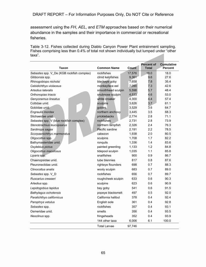
DRAFT REPORT – For Information Purposes Only, Do NOT Cite or Reference
65
assessment using the FH, AEL, and ETM approaches based on their numerical abundance in the samples and their importance in commercial or recreational fisheries.
Table 3-12. Fishes collected during Diablo Canyon Power Plant entrainment sampling. Fishes comprising less than 0.4% of total not shown individually but lumped under “other taxa”.
Taxon Common Name Count Percent of
Total Cumulative
Percent Sebastes spp. V_De (KGB rockfish complex) rockfishes 17,576 18.0 18.0 Gibbonsia spp. clinid kelpfishes 9,361 9.6 27.6 Rhinogobiops nicholsi blackeye goby 7,658 7.8 35.4 Cebidichthys violaceus monkeyface eel 7,090 7.3 42.6 Artedius lateralis smoothhead sculpin 5,598 5.7 48.4 Orthonopias triacis snubnose sculpin 4,533 4.6 53.0 Genyonemus lineatus white croaker 4,300 4.4 57.4 Cottidae unid. sculpins 3,626 3.7 61.1 Gobiidae unid. gobies 3,529 3.6 64.7 Engraulis mordax northern anchovy 3,445 3.5 68.3 Stichaeidae unid. pricklebacks 2,774 2.8 71.1 Sebastes spp. V (blue rockfish complex) rockfishes 2,731 2.8 73.9 Stenobrachius leucopsarus northern lampfish 2,326 2.4 76.3 Sardinops sagax Pacific sardine 2,191 2.2 78.5 Scorpaenichthys marmoratus cabezon 1,938 2.0 80.5 Oligocottus spp. sculpins 1,708 1.7 82.2 Bathymasteridae unid. ronquils 1,336 1.4 83.6 Oxylebius pictus painted greenling 1,133 1.2 84.8 Oligocottus maculosus tidepool sculpin 1,035 1.1 85.8 Liparis spp. snailfishes 900 0.9 86.7 Chaenopsidae unid. tube blennies 817 0.8 87.6 Pleuronectidae unid. righteye flounders 698 0.7 88.3 Clinocottus analis wooly sculpin 683 0.7 89.0 Sebastes spp. V_D rockfishes 656 0.7 89.7 Ruscarius creaseri roughcheek sculpin 633 0.6 90.3 Artedius spp. sculpins 623 0.6 90.9 Lepidogobius lepidus bay goby 541 0.6 91.5 Bathylagus ochotensis popeye blacksmelt 497 0.5 92.0 Paralichthys californicus California halibut 378 0.4 92.4 Parophrys vetulus English sole 361 0.4 92.8 Sebastes spp. rockfishes 357 0.4 93.1 Osmeridae unid. smelts 356 0.4 93.5 Neoclinus spp. fringeheads 352 0.4 93.9 144 other taxa 6,006 6.1 100.0
Total Larvae 97,746
DRAFT REPORT – For Information Purposes Only, Do NOT Cite or Reference
66
There were 43,785 larval fishes identified and enumerated from the 3,163 samples processed from the nearshore sampling area. These comprised 175 different taxa ranging from ordinal to specific levels of classification. Adults of these taxa live in a variety of habitats, from intertidal and shallow subtidal to deep-water and pelagic habitats. The taxa in highest abundance in the nearshore sampling area were those whose adults were typically pelagic or subtidal; the more intertidally or nearshore distributed species were found in lower abundance in the sampling area.
DCPP Results for the KGB Rockfish Complex Larval rockfishes in the KGB complex showed distinct seasonal peaks of
abundance at the DCPP intake structure, with their greatest abundance tending to occur between March and July (Figure 3-6). An El Niño began developing during the spring of 1997 (NOAA 1999) and was detected along the coast of California in fall of that year (Lynn et al. 1998). This may have slightly affected the density in 1998 compared with the previous year. The El Niño event did not affect seasonal peaks in abundance between years; during both periods KGB rockfish larvae first starting appearing in February, reached peak abundances in April-May, and were not present following late-July.
There were 17,863 larval KGB rockfishes identified from 774 of samples collected at the DCPP intake structure between October 1996 and June 1999 representing 20% of the entrainment samples collected and processed during that period. Annual estimated numbers of KGB rockfish larvae entrained at DCPP varied relatively little between the 1996–97 Analysis Period 1 (268,000,000) and the 1997–98 Analysis Period 2 (199,000,000) (Table 3-13). An approximation of 95% confidence intervals (± 2 std. errors) for the two estimates overlap indicating that the differences between them were probably not statistically significant and that entrainment of KGB rockfish larvae was relatively constant between years.
Estimates of annually entrained KGB rockfish larvae were adjusted (Table 3-13) to the long-term average DCPP Intake Cove surface plankton tow index, calculated as the ratio between the 9 yr average of DCPP Intake Cove sampling (Figure 3-7) and the average annual index estimated from these same tows during the year being adjusted. Average indices for the years 1997 and 1998 were 0.070 and 0.065 larvae/m3, respectively, and the long-term average index for 1990–98 was 0.072 larvae/m3. Thus, the ratios used to adjust the 1997 and 1998 estimates of larvae entrained were 1.03 and 1.13, respectively, indicating that larval density was slightly lower than the long-term average during
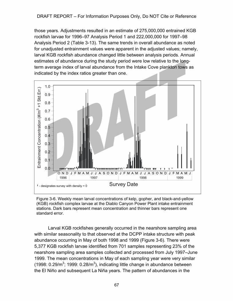
DRAFT REPORT – For Information Purposes Only, Do NOT Cite or Reference
67
those years. Adjustments resulted in an estimate of 275,000,000 entrained KGB rockfish larvae for 1996–97 Analysis Period 1 and 222,000,000 for 1997–98 Analysis Period 2 (Table 3-13). The same trends in overall abundance as noted for unadjusted entrainment values were apparent in the adjusted values; namely, larval KGB rockfish abundance changed little between analysis periods. Annual estimates of abundance during the study period were low relative to the long-term average index of larval abundance from the Intake Cove plankton tows as indicated by the index ratios greater than one.
Figure 3-6. Weekly mean larval concentrations of kelp, gopher, and black-and-yellow (KGB) rockfish complex larvae at the Diablo Canyon Power Plant intake entrainment stations. Dark bars represent mean concentration and thinner bars represent one standard error.
Larval KGB rockfishes generally occurred in the nearshore sampling area with similar seasonality to that observed at the DCPP intake structure with peak abundance occurring in May of both 1998 and 1999 (Figure 3-6). There were 5,377 KGB rockfish larvae identified from 701 samples representing 23% of the nearshore sampling area samples collected and processed from July 1997–June 1999. The mean concentrations in May of each sampling year were very similar (1998: 0.29/m3; 1999: 0.28/m3), indicating little change in abundance between the El Niño and subsequent La Niña years. The pattern of abundances in the
1996 1997 1998 1999
- designates survey with density = 0
0.0
0.1
0.2
0.3
0.4
0.5
0.6
0.7
0.8
0.9
1.0
Survey Date
Ent
rain
men
t Con
cent
ratio
n (#
/m +
1 St
d.E
rr.)
3
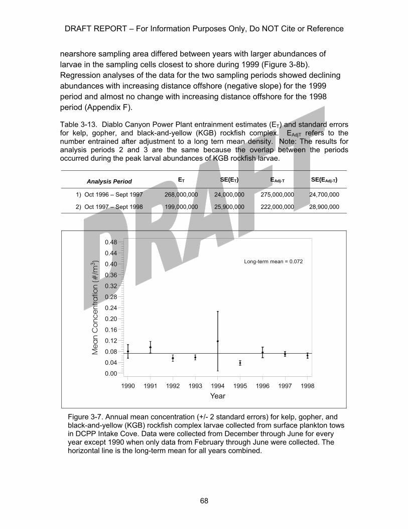
DRAFT REPORT – For Information Purposes Only, Do NOT Cite or Reference
68
nearshore sampling area differed between years with larger abundances of larvae in the sampling cells closest to shore during 1999 (Figure 3-8b). Regression analyses of the data for the two sampling periods showed declining abundances with increasing distance offshore (negative slope) for the 1999 period and almost no change with increasing distance offshore for the 1998 period (Appendix F).
Table 3-13. Diablo Canyon Power Plant entrainment estimates (ET) and standard errors for kelp, gopher, and black-and-yellow (KGB) rockfish complex. EAdjT refers to the number entrained after adjustment to a long tern mean density. Note: The results for analysis periods 2 and 3 are the same because the overlap between the periods occurred during the peak larval abundances of KGB rockfish larvae.
Analysis Period ET SE(ET) EAdj-T SE(EAdj-T)
1) Oct 1996 – Sept 1997 268,000,000 24,000,000 275,000,000 24,700,000
2) Oct 1997 – Sept 1998 199,000,000 25,900,000 222,000,000 28,900,000
Figure 3-7. Annual mean concentration (+/- 2 standard errors) for kelp, gopher, and black-and-yellow (KGB) rockfish complex larvae collected from surface plankton tows in DCPP Intake Cove. Data were collected from December through June for every year except 1990 when only data from February through June were collected. The horizontal line is the long-term mean for all years combined.
Long-term mean = 0.072
0.00
0.04
0.08
0.12
0.16
0.20
0.24
0.28
0.32
0.36
0.40
0.44
0.48
Year1990 1991 1992 1993 1994 1995 1996 1997 1998
Me
an
Co
nce
ntra
tion
(#/m
)3
DRAFT REPORT – For Information Purposes Only, Do NOT Cite or Reference
69
Standard lengths of all measured KGB rockfish larvae collected at the DCPP intake structure between October 1996 and June 1999 (9,926 larvae) ranged from 2.4 to 8.0 mm (mean = 4.2 mm) (Figure 3-9). The lengths of entrained KGB larvae, excluding the largest 1% and smallest 1% of all measurements, ranged from 3.3 to 5.6 mm. Similar to the KGB assessment at Morro Bay, a growth rate of 0.14 mm/d (Mary Yoklavich, NOAA / NMFS / PFEG, Santa Cruz, CA, pers. comm. 1999) was used to estimate the age of entrained larvae. Assuming that the size of the smallest 1% represents post-extrusion larvae that are aged zero days, then the estimated ages of entrained larvae ranged from zero up to ca. 16.4 d post-extrusion for the size of the largest 1% of the larvae. The estimated average age of KGB larvae entrained at DCPP was 6.4 d post-extrusion. The reported extrusion size for species in this complex ranges from 4.0–5.5 mm (Moser 1996).
Fecundity Hindcasting
The same life history parameter values used for the MBPP study (Table 3-8) were also used to calculate FH estimates for the KGB rockfish complex for the DCPP study. Average age at entrainment was estimated as 6.2 d. This was calculated by subtracting the value of the 1st percentile value of the lengths (3.3 mm) from the mean length at entrainment (4.2 mm) and dividing by the larval growth rate for brown rockfish of 0.14 mm/d (Love and Johnson 1999; Yoklavich et al. 1996) that was also used in the MBPP study. The survival rate of the KGB larvae from size at entrainment to size at recruitment into the fishery was partitioned into six stages from parturition to recruitment using the same approach presented for the MBPP study (Table 3-14). The survival rate from extrusion to the average age at entrainment using data from blue rockfish was estimated as 0.419 (0.419 = e(-0.14)(6.2)).
The estimated number of adult KGB rockfish females at the age of maturity whose reproductive output was been lost due to entrainment was 617 for the 1996–97 period and 497 for the 1997–98 period (Table 3-14). The similarity between the estimates was a direct result of the similarity between adjusted entrainment estimates for the two periods. Low FH estimates resulted from the relatively high fecundity of adults and young average entrainment age estimated for larvae in this complex and not including other sources of mortality such as losses due to fishing in the model. The variation in the entrainment estimate had very little effect on the model estimates relative to the variation resulting from the life history parameters.
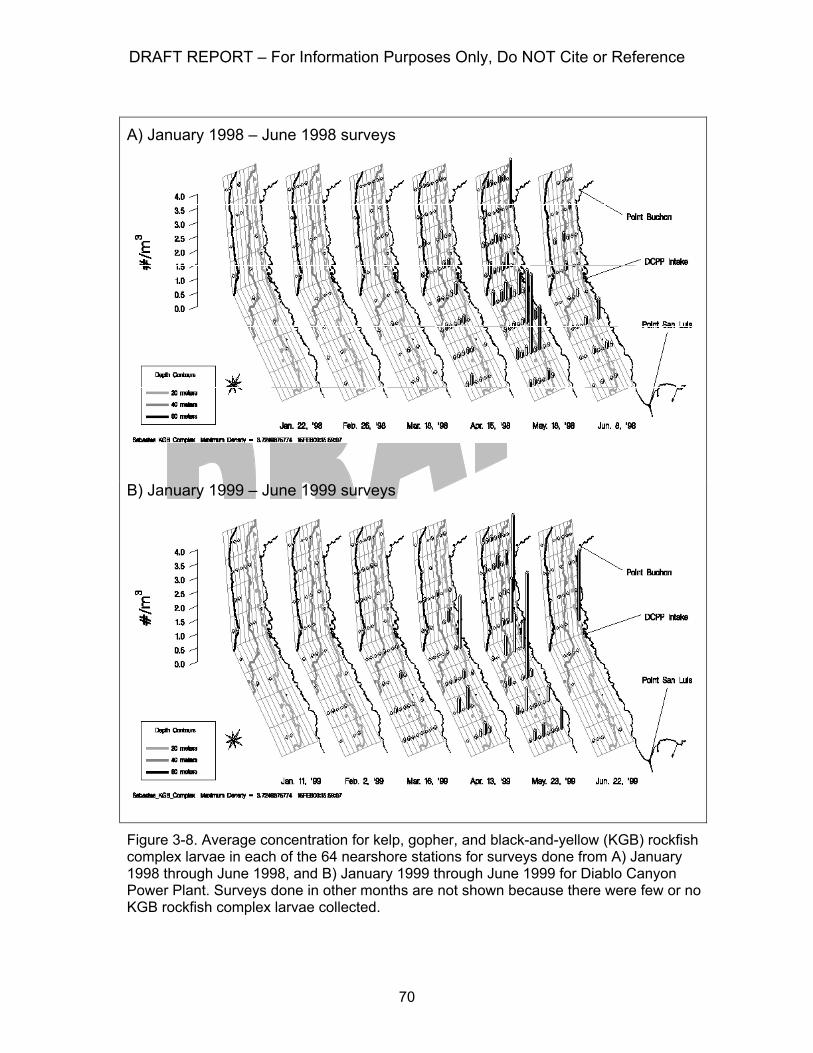
DRAFT REPORT – For Information Purposes Only, Do NOT Cite or Reference
70
A) January 1998 – June 1998 surveys
B) January 1999 – June 1999 surveys
Figure 3-8. Average concentration for kelp, gopher, and black-and-yellow (KGB) rockfish complex larvae in each of the 64 nearshore stations for surveys done from A) January 1998 through June 1998, and B) January 1999 through June 1999 for Diablo Canyon Power Plant. Surveys done in other months are not shown because there were few or no KGB rockfish complex larvae collected.
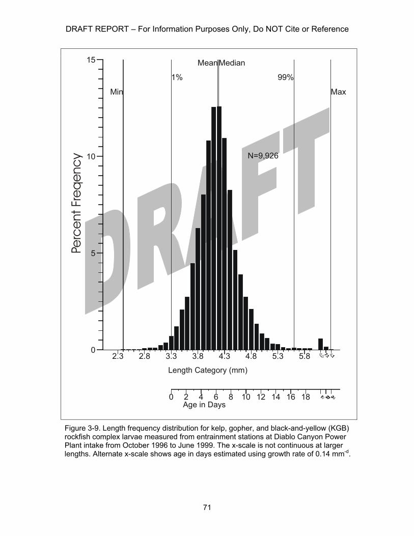
DRAFT REPORT – For Information Purposes Only, Do NOT Cite or Reference
71
Figure 3-9. Length frequency distribution for kelp, gopher, and black-and-yellow (KGB) rockfish complex larvae measured from entrainment stations at Diablo Canyon Power Plant intake from October 1996 to June 1999. The x-scale is not continuous at larger lengths. Alternate x-scale shows age in days estimated using growth rate of 0.14 mm-d.
Min
1%
MeanMedian
99%
Max
0 2 4 6 8 10 12 14 16 18
N=9,926
0
5
10
15
2.3 2.8 3.3 3.8 4.3 4.8 5.3 5.8
Length Category (mm)
Age in Days
Perc
ent
Fre
qe
ncy
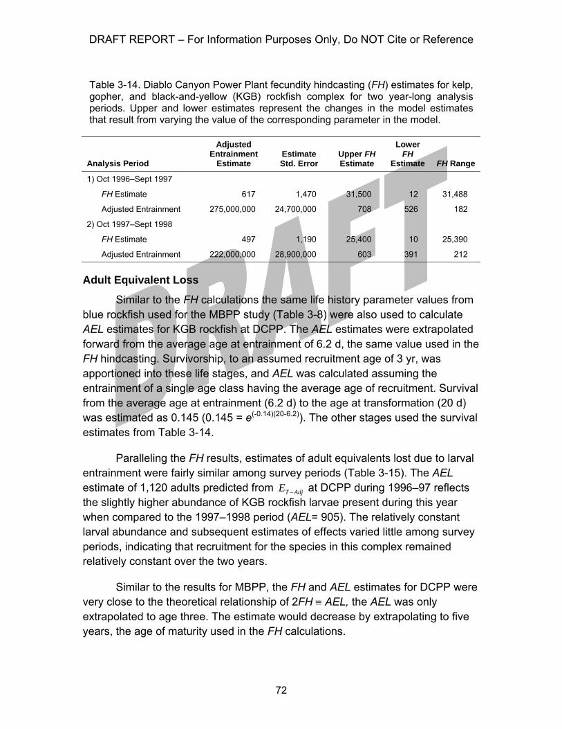
DRAFT REPORT – For Information Purposes Only, Do NOT Cite or Reference
72
Table 3-14. Diablo Canyon Power Plant fecundity hindcasting (FH) estimates for kelp, gopher, and black-and-yellow (KGB) rockfish complex for two year-long analysis periods. Upper and lower estimates represent the changes in the model estimates that result from varying the value of the corresponding parameter in the model.
Analysis Period
Adjusted Entrainment
Estimate Estimate Std. Error
Upper FH Estimate
Lower FH
Estimate FH Range
1) Oct 1996–Sept 1997
FH Estimate 617 1,470 31,500 12 31,488
Adjusted Entrainment 275,000,000 24,700,000 708 526 182
2) Oct 1997–Sept 1998
FH Estimate 497 1,190 25,400 10 25,390
Adjusted Entrainment 222,000,000 28,900,000 603 391 212
Adult Equivalent Loss
Similar to the FH calculations the same life history parameter values from blue rockfish used for the MBPP study (Table 3-8) were also used to calculate AEL estimates for KGB rockfish at DCPP. The AEL estimates were extrapolated forward from the average age at entrainment of 6.2 d, the same value used in the FH hindcasting. Survivorship, to an assumed recruitment age of 3 yr, was apportioned into these life stages, and AEL was calculated assuming the entrainment of a single age class having the average age of recruitment. Survival from the average age at entrainment (6.2 d) to the age at transformation (20 d) was estimated as 0.145 (0.145 = e(-0.14)(20-6.2)). The other stages used the survival estimates from Table 3-14.
Paralleling the FH results, estimates of adult equivalents lost due to larval entrainment were fairly similar among survey periods (Table 3-15). The AEL estimate of 1,120 adults predicted from T AdjE − at DCPP during 1996–97 reflects the slightly higher abundance of KGB rockfish larvae present during this year when compared to the 1997–1998 period (AEL= 905). The relatively constant larval abundance and subsequent estimates of effects varied little among survey periods, indicating that recruitment for the species in this complex remained relatively constant over the two years.
Similar to the results for MBPP, the FH and AEL estimates for DCPP were very close to the theoretical relationship of 2FH ≡ AEL, the AEL was only extrapolated to age three. The estimate would decrease by extrapolating to five years, the age of maturity used in the FH calculations.
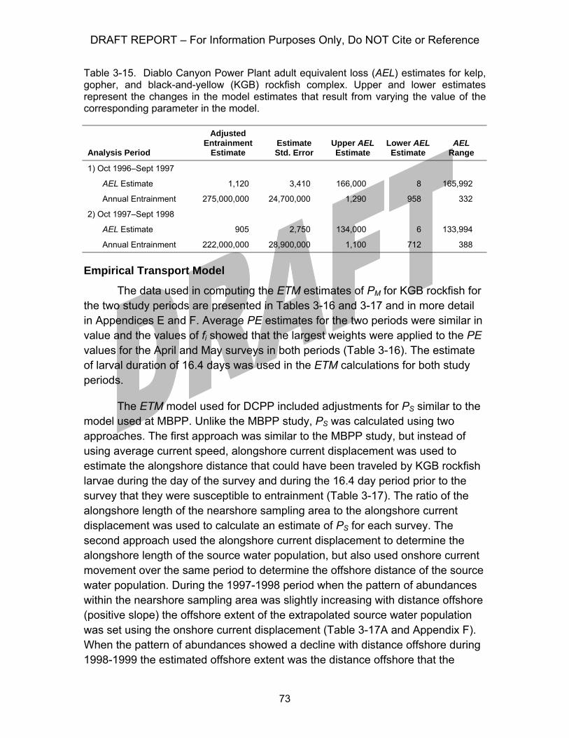
DRAFT REPORT – For Information Purposes Only, Do NOT Cite or Reference
73
Table 3-15. Diablo Canyon Power Plant adult equivalent loss (AEL) estimates for kelp, gopher, and black-and-yellow (KGB) rockfish complex. Upper and lower estimates represent the changes in the model estimates that result from varying the value of the corresponding parameter in the model.
Analysis Period
Adjusted Entrainment
Estimate Estimate Std. Error
Upper AEL Estimate
Lower AEL Estimate
AEL Range
1) Oct 1996–Sept 1997
AEL Estimate 1,120 3,410 166,000 8 165,992
Annual Entrainment 275,000,000 24,700,000 1,290 958 332
2) Oct 1997–Sept 1998
AEL Estimate 905 2,750 134,000 6 133,994
Annual Entrainment 222,000,000 28,900,000 1,100 712 388
Empirical Transport Model
The data used in computing the ETM estimates of PM for KGB rockfish for the two study periods are presented in Tables 3-16 and 3-17 and in more detail in Appendices E and F. Average PE estimates for the two periods were similar in value and the values of fi showed that the largest weights were applied to the PE values for the April and May surveys in both periods (Table 3-16). The estimate of larval duration of 16.4 days was used in the ETM calculations for both study periods.
The ETM model used for DCPP included adjustments for PS similar to the model used at MBPP. Unlike the MBPP study, PS was calculated using two approaches. The first approach was similar to the MBPP study, but instead of using average current speed, alongshore current displacement was used to estimate the alongshore distance that could have been traveled by KGB rockfish larvae during the day of the survey and during the 16.4 day period prior to the survey that they were susceptible to entrainment (Table 3-17). The ratio of the alongshore length of the nearshore sampling area to the alongshore current displacement was used to calculate an estimate of PS for each survey. The second approach used the alongshore current displacement to determine the alongshore length of the source water population, but also used onshore current movement over the same period to determine the offshore distance of the source water population. During the 1997-1998 period when the pattern of abundances within the nearshore sampling area was slightly increasing with distance offshore (positive slope) the offshore extent of the extrapolated source water population was set using the onshore current displacement (Table 3-17A and Appendix F). When the pattern of abundances showed a decline with distance offshore during 1998-1999 the estimated offshore extent was the distance offshore that the
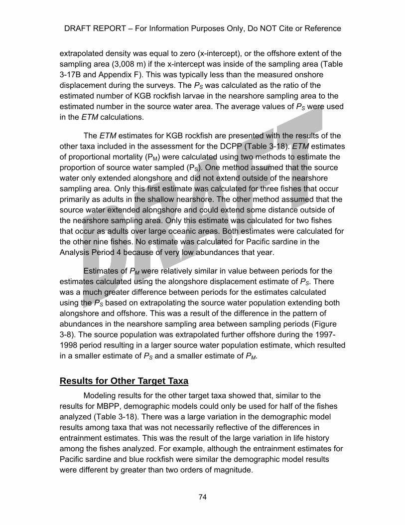
DRAFT REPORT – For Information Purposes Only, Do NOT Cite or Reference
74
extrapolated density was equal to zero (x-intercept), or the offshore extent of the sampling area (3,008 m) if the x-intercept was inside of the sampling area (Table 3-17B and Appendix F). This was typically less than the measured onshore displacement during the surveys. The PS was calculated as the ratio of the estimated number of KGB rockfish larvae in the nearshore sampling area to the estimated number in the source water area. The average values of PS were used in the ETM calculations.
The ETM estimates for KGB rockfish are presented with the results of the other taxa included in the assessment for the DCPP (Table 3-18). ETM estimates of proportional mortality (PM) were calculated using two methods to estimate the proportion of source water sampled (PS). One method assumed that the source water only extended alongshore and did not extend outside of the nearshore sampling area. Only this first estimate was calculated for three fishes that occur primarily as adults in the shallow nearshore. The other method assumed that the source water extended alongshore and could extend some distance outside of the nearshore sampling area. Only this estimate was calculated for two fishes that occur as adults over large oceanic areas. Both estimates were calculated for the other nine fishes. No estimate was calculated for Pacific sardine in the Analysis Period 4 because of very low abundances that year.
Estimates of PM were relatively similar in value between periods for the estimates calculated using the alongshore displacement estimate of PS. There was a much greater difference between periods for the estimates calculated using the PS based on extrapolating the source water population extending both alongshore and offshore. This was a result of the difference in the pattern of abundances in the nearshore sampling area between sampling periods (Figure 3-8). The source population was extrapolated further offshore during the 1997-1998 period resulting in a larger source water population estimate, which resulted in a smaller estimate of PS and a smaller estimate of PM.
Results for Other Target Taxa Modeling results for the other target taxa showed that, similar to the
results for MBPP, demographic models could only be used for half of the fishes analyzed (Table 3-18). There was a large variation in the demographic model results among taxa that was not necessarily reflective of the differences in entrainment estimates. This was the result of the large variation in life history among the fishes analyzed. For example, although the entrainment estimates for Pacific sardine and blue rockfish were similar the demographic model results were different by greater than two orders of magnitude.
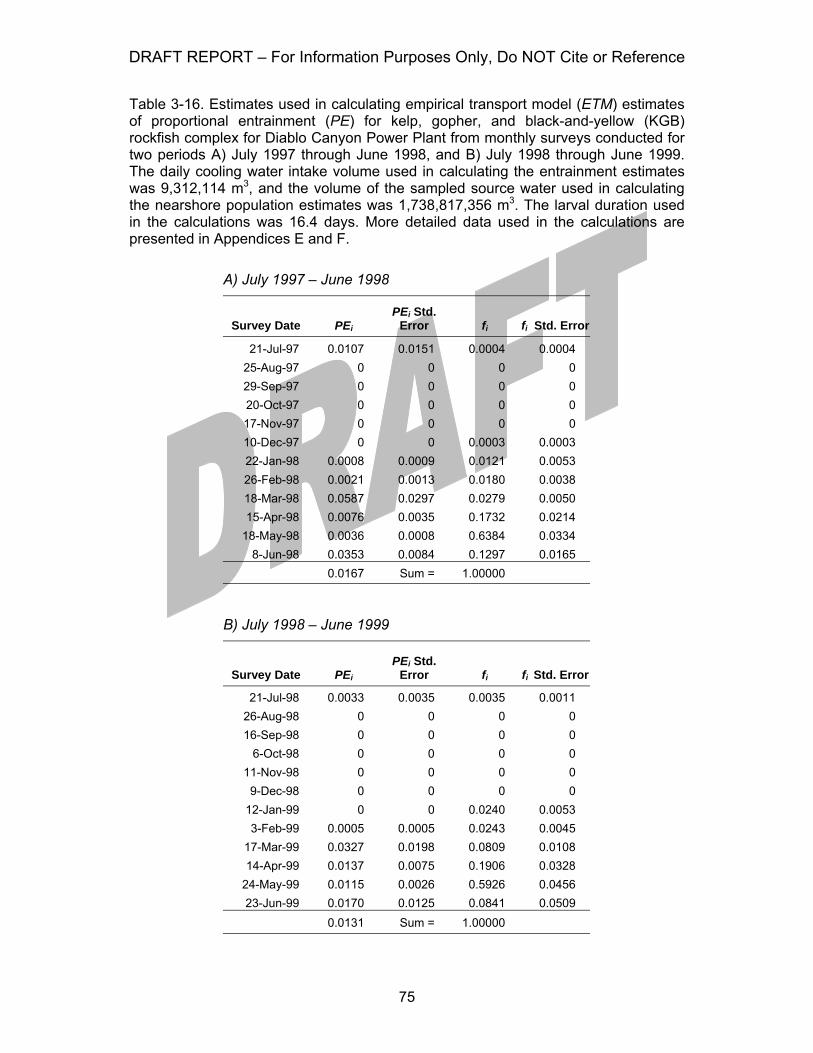
DRAFT REPORT – For Information Purposes Only, Do NOT Cite or Reference
75
Table 3-16. Estimates used in calculating empirical transport model (ETM) estimates of proportional entrainment (PE) for kelp, gopher, and black-and-yellow (KGB) rockfish complex for Diablo Canyon Power Plant from monthly surveys conducted for two periods A) July 1997 through June 1998, and B) July 1998 through June 1999. The daily cooling water intake volume used in calculating the entrainment estimates was 9,312,114 m3, and the volume of the sampled source water used in calculating the nearshore population estimates was 1,738,817,356 m3. The larval duration used in the calculations was 16.4 days. More detailed data used in the calculations are presented in Appendices E and F.
A) July 1997 – June 1998
Survey Date PEi PEi Std.
Error fi fi Std. Error
21-Jul-97 0.0107 0.0151 0.0004 0.0004 25-Aug-97 0 0 0 0 29-Sep-97 0 0 0 0 20-Oct-97 0 0 0 0 17-Nov-97 0 0 0 0 10-Dec-97 0 0 0.0003 0.0003 22-Jan-98 0.0008 0.0009 0.0121 0.0053 26-Feb-98 0.0021 0.0013 0.0180 0.0038 18-Mar-98 0.0587 0.0297 0.0279 0.0050 15-Apr-98 0.0076 0.0035 0.1732 0.0214
18-May-98 0.0036 0.0008 0.6384 0.0334 8-Jun-98 0.0353 0.0084 0.1297 0.0165
0.0167 Sum = 1.00000
B) July 1998 – June 1999
Survey Date PEi PEi Std.
Error fi fi Std. Error
21-Jul-98 0.0033 0.0035 0.0035 0.0011 26-Aug-98 0 0 0 0 16-Sep-98 0 0 0 0
6-Oct-98 0 0 0 0 11-Nov-98 0 0 0 0 9-Dec-98 0 0 0 0
12-Jan-99 0 0 0.0240 0.0053 3-Feb-99 0.0005 0.0005 0.0243 0.0045
17-Mar-99 0.0327 0.0198 0.0809 0.0108 14-Apr-99 0.0137 0.0075 0.1906 0.0328
24-May-99 0.0115 0.0026 0.5926 0.0456 23-Jun-99 0.0170 0.0125 0.0841 0.0509
0.0131 Sum = 1.00000

DRAFT REPORT – For Information Purposes Only, Do NOT Cite or Reference
76
Table 3-17. Onshore and alongshore current meter displacement used in estimating proportion of source water sampled (PS) from monthly surveys conducted for two periods A) July 1997 through June 1998, and B) July 1998 through June 1999 for kelp, gopher, and black-and-yellow (KGB) rockfish complex at the Diablo Canyon Power Plant. More detailed data including regression coefficients and population estimates included in Appendices E and F.
A) July 1997 – June 1998
Survey Date
Cumulative Alongshore
Displacement (m)
Onshore Current
Displacement (m)
Estimated Offshore Extent of
Source Water (m)
Offshore PS
Alongshore PS
21-Jul-97 31,300 4,820 4,820 0.0153 0.5545 25-Aug-97 − − − − − 29-Sep-97 − − − − − 20-Oct-97 − − − − − 17-Nov-97 − − − − − 10-Dec-97 146,000 31,600 31,600 0.0000 0.1189 22-Jan-98 120,000 23,400 23,400 0.0020 0.1443 26-Feb-98 33,700 8,710 8,710 0.0693 0.5152 18-Mar-98 181,000 12,400 12,400 0.0090 0.0960 15-Apr-98 76,100 12,800 12,800 0.0404 0.2282
18-May-98 67,100 19,900 19,900 0.0334 0.2589 8-Jun-98 111,000 5,670 5,670 0.0761 0.1559
0.0307 0.2590
B) July 1998 - June 1998
Survey Date
Cumulative Alongshore
Displacement (m)
Onshore Current
Displacement (m)
Estimated Offshore Extent of
Source Water (m)
Offshore PS
Alongshore PS
21-Jul-98 76,300 11,100 3,010 0.2278 0.2278 26-Aug-98 − − − − − 16-Sep-98 − − − − −
6-Oct-98 − − − − − 11-Nov-98 − − − − − 9-Dec-98 − − − − −
12-Jan-99 46,200 24,100 3,010 0.3755 0.3755 3-Feb-99 81,900 19,700 3,010 0.2122 0.2122
17-Mar-99 36,900 8,540 4,170 0.4334 0.4709 14-Apr-99 163,000 10,200 8,000 0.0636 0.1068
24-May-99 180,000 21,800 21,000 0.0251 0.0967 23-Jun-99 158,000 5,970 4,380 0.0986 0.1100
0.2052 0.2286
DRAFT REPORT – For Information Purposes Only, Do NOT Cite or Reference
77
The fishes analyzed were separated into three groups based on their adult distributions: fishes that were widely distributed over large oceanic areas included northern anchovy and Pacific sardine, fishes that were primarily distributed in the shallow nearshore included smoothhead sculpin (Orthonopias triacis), monkeyface prickleback (Cebidichthys violaceus), and clinid kelpfishes (Gibbonsia spp.), and the rest of the fishes that were primarily nearshore, but could be found in deeper subtidal areas. The source water population used in calculating PS was estimated using both alongshore currents and along- and off-shore extrapolation for the last group of fishes resulting in two ETM estimates for each analysis period. Only one ETM estimate for each analysis period was made for the other two groups depending on whether it was primarily nearshore, or primarily offshore. The ETM estimates of PM ranged from <0.001 (0.1%) to 0.310 (31.0%) with the estimated effects being greatest for the fishes that were distributed primarily as adults in shallow nearshore areas. These fishes such as sculpins (Cottidae), monkeyface pricklebacks, and kelpfishes all had proportional mortalities due to power plant entrainment of greater than 10%. The ETM calculations were calculated using both estimates of PS for snubnose sculpin because they occur slightly deeper as adults than the other nearshore fishes. The results showed that the extrapolated ETM estimates were approximately equal to the estimates using only alongshore current displacement because the densities for this species did not increase with distance offshore. The results for DCPP are similar to the other two studies in showing that the greatest effects occur to fishes that primarily occupy habitats in close proximity to the intake and do not occur at the same level in other areas of the source water.
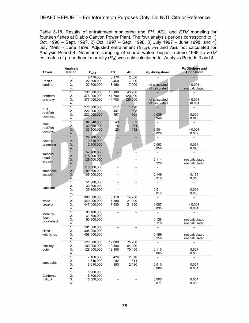
DRAFT REPORT – For Information Purposes Only, Do NOT Cite or Reference
78
Table 3-18. Results of entrainment monitoring and FH, AEL, and ETM modeling for fourteen fishes at Diablo Canyon Power Plant. The four analysis periods correspond to 1) Oct. 1996 – Sept. 1997, 2) Oct. 1997 – Sept. 1998, 3) July 1997 – June 1998, and 4) July 1998 – June 1999. Adjusted entrainment (EAdjT), FH and AEL not calculated for Analysis Period 4. Nearshore sampling of source waters began in June 1998 so ETM estimates of proportional mortality (PM) was only calculated for Analysis Periods 3 and 4.
Taxon
Analysis Period Eadj-T FH AEL PM Alongshore
PM Offshore and Alongshore
Pacific sardine
1. 2. 3. 4.
8,470,00022,600,00022,600,000
3,1708,4608,460
2,6307,0007,000
− −
not calculated not calculated
− −
<0.001 not calculated
northern anchovy
1. 2. 3. 4.
136,000,000376,000,000377,000,000
16,10044,70044,700
43,200120,000120,000
− −
not calculated not calculated
− −
<0.001 <0.001
KGB rockfish complex
1. 2. 3. 4.
275,000,000222,000,000222,000,000
617497497
1,120905905
− −
0.039 0.048
− −
0.005 0.043
blue rockfish complex
1. 2. 3. 4.
84,040,00033,800,00033,900,000
431820
353164142
− −
0.004 0.028
− −
<0.001 0.002
painted greenling
1. 2. 3. 4.
24,200,0009,610,000
12,100,000
−−−
−−−
− −
0.063 0.056
− −
0.051 0.043
smooth-head sculpin
1. 2. 3. 4.
57,700,000115,000,000129,000,000
−−−
−−−
− −
0.114 0.226
− −
not calculated not calculated
snubnose sculpin
1. 2. 3. 4.
110,000,00083,500,000
105,000,000
−−−
−−−
− −
0.149 0.310
− −
0.139 0.310
cabezon
1. 2. 3. 4,
51,900,00036,300,00036,300,000
−−−
−−−
− −
0.011 0.015
− −
0.009 0.008
white croaker
1. 2. 3. 4.
305,000,000440,000,000447,000,000
5,1107,3807,500
14,70021,30021,600
− −
0.007 0.035
− −
<0.001 0.004
Monkey-face prickleback
1. 2. 3. 4.
83,100,00061,500,00060,200,000
−−−
−−−
− −
0.138 0.118
− −
not calculated not calculated
clinid kelpfishes
1. 2. 3. 4.
181,000,000308,000,000458,000,000
−−−
−−−
− −
0.189 0.250
− −
not calculated not calculated
blackeye goby
1. 2. 3. 4.
128,000,000109,000,000128,000,000
12,00010,30012,100
75,20064,10075,400
− −
0.115 0.065
− −
0.027 0.036
sanddabs
1. 2. 3. 4.
7,160,0001,540,0006,610,000
42692
393
2,370511
2,190
− −
0.010 0.008
− −
0.001 0.001
California halibut
1. 2. 3. 4.
8,260,00015,700,00015,500,000
−−−
−−−
− −
0.005 0.071
− −
0.001 0.006
DRAFT REPORT – For Information Purposes Only, Do NOT Cite or Reference
79
4.0 DISCUSSION
The results from these studies demonstrate the importance of a site-specific approach to assessing the effects of CWIS entrainment on marine organisms. Even though Morro Bay and San Diego Bay are both tidally influenced embayments the resulting studies, sampling, and analytical approaches were very different. And both of these studies were dramatically different from Diablo Canyon. The source waters determined to be affected by entrainment were the primary factor responsible for the differences among studies. In San Diego Bay, in the area of SBPP, the turnover in water due to tidal exchange allowed us to treat the source water population as a close system. A larger number of stations was sampled in San Diego compared to Morro Bay because of the potential for reduced exchange among the various habitats in the San Diego source water study area. Differences in fish composition among habitats in San Diego Bay shown by Allen (1999) were also reflected in some of the differences in larval composition among stations (Table 7). This resulted in site-specific effects on species such as longjaw mudsuckers which had a relatively high ETM estimate of PM at SBPP. Mudsucker larvae were not particularly abundant in the source waters but were abundant in the SBPP intake canal which provided excellent habitat for adults. Similarly, effects on combtooth blennies estimated using ETM were lower than other fishes because they were more abundant in areas of the bay that had extensive pier pilings and other structures that provide habitat for adult blennies. The high level of site fidelity in the community composition in south San Diego Bay was likely due to the lower tidal exchange rates relative to an area such as Morro Bay. The results supported our decision to sample an extensive range of habitats in south San Diego Bay.
The source water sampling in Morro Bay was less extensive than the SBPP study, but included sampling at a nearshore station outside of the bay that was representative of water transported into the bay on flood tides. The less intensive sampling was justified by the large tidal exchange that results in rapid turnover of the water in the bay relative to a large tidal embayment such as San Diego Bay. The shallow mudflats and tidal channels in Morro Bay are drained out through the deeper navigation channel where sampling occurred. Although this may have resulted in under-sampling of larvae from certain fishes that could avoid strong tidal currents, as has been shown for longjaw mudsuckers and other species of gobies (Barlow 1963, Brothers 1975), it was probably representative of the larvae that would be transported on outgoing tides past the plant where they would be exposed to entrainment. The greatest CWIS effects using ETM were estimated for combtooth blennies that occur in the piers and other
DRAFT REPORT – For Information Purposes Only, Do NOT Cite or Reference
80
structures located near the plant. This was similar to the SBPP results for longjaw mudsuckers that occur in highest numbers at the entrainment station in the intake canal. These results showed the importance of sampling all habitats and the potential for increased impacts on species with habitats near plant intakes. This also indicates that potential for large impacts exist when habitats are not uniformly distributed in the source water for a CWIS and the potential for larger effects on fishes associated with habitats that may not be abundant throughout the source water.
The nearshore sampling area for DCPP was very extensive to represent the range of habitats along the exposed rocky headland where the power plant is located. The size of the sampling area was also designed to be representative of the distance north and south that larvae could be transported by alongshore currents over a 24 hour period to correspond with the ETM model that uses daily estimates of conditional mortality resulting from entrainment to estimate CWIS-related mortality. This extensive sampling showed similar results to SBPP and MBPP by estimating that the greatest CWIS effects using ETM occurred on fishes with nearshore habitats that were disproportionately affected by entrainment. In the ETM model species that have higher abundances in entrainment samples results in larger PE estimates of daily conditional mortality.
We examined the relative distribution of individual species in the sampling areas by comparing the average PE to the ratio of the cooling water to source water volumes. For example, in SBPP the average PE for CIQ gobies was 0.012 which was very close to the volumetric ratio of 0.015. In contrast, the average PE for longjaw mudsuckers was 0.19 which was much greater than the ratio of cooling water to source water. Although this is potentially useful for helping to determine the potential distribution of the larvae in the source water it may not be a good indicator of impacts. When the PE is close to the volumetric ratio the resulting impacts are directly dependent on the number of days that the larvae are exposed to entrainment. Therefore, even though the average PE was much greater for longjaw mudsuckers, the time (4 days) that they were exposed to entrainment was much less than CIQ gobies because they were in highest abundance in the areas directly around the CWS intake. In contrast, even though the average PE for CIQ goby was close to the volumetric ratio, the estimated effects of entrainment based on ETM were higher than the estimated effects on mudsuckers (0.215 vs. 0.171) because goby larvae were estimated to be exposed to entrainment for 23 days.
The final source water area used to adjust the PE estimates also affected the CWIS effects estimated using ETM. The MBPP results for KGB rockfish
DRAFT REPORT – For Information Purposes Only, Do NOT Cite or Reference
81
contrast with those for estuarine fishes such as gobies and blennies. Relative to fishes that are primarily estuarine inhabitants, adult KGB rockfishes are more widely distributed resulting in larger source water body populations and reduced entrainment effects. As a result the PE estimates were adjusted using PS to account for the larger source water population beyond the area sampled for KGB rockfishes. All of the results for DCPP were adjusted to account for the onshore and alongshore currents that can transport larvae over hundreds of kilometers, resulting in very low estimated effects for species, such as northern anchovy, that have widely distributed source populations.
The source water sampling for all three of these studies was done to satisfy the requirements of the ETM. Source water sampling would not have been required if the assessments were done using only more traditional demographic modeling approaches. The source water sampling was necessary because the ETM directly links mortality to a source population. As a consequence, the habitat occupied by that source population can be described and ecosystem losses can be mitigated. The area of production foregone (APF) is one approach for estimating the amount of habitat that would need to be replaced to compensate for the larval production lost due to entrainment. The APF is estimated as the product of PM and the source water area for each “target” species. The APF needs to be scaled to the area of the habitat in the source water for species that occupy very specific habitats. For example, if the area of mudflat habitat in an estuary is 5,000 hectares and the entrainment mortality (PM) for CIQ gobies that primarily occupy mudflat habitat is 0.10 (10%), the APF estimate is 500 hectares even though the total area of the estuary may be much larger. This approach becomes more difficult on the open coast where areas of rocky vs. sandy habitat would need to be estimated and depth distributions for impacted species would need to be accounted for. It is also difficult for species that are cosmopolitan in distribution. This task is simplified by the proportional relationship between PM and the size of the source water population used in calculating PS. As the size of the source water area increases relative to the sampling area, PS decreases resulting in a proportional decrease in PM. If the habitat in the larger source water can be assumed to be distributed in the same relative proportions as the area sampled then you only need to use the areas of various habitats in the sampled area to estimate APF by using the uncorrected PM. This greatly simplifies the application of APF and also reduces the need to rely on limited current data information to extrapolate beyond the areas sampled. In practice, when many species are impacted, each having varying habitat requirements, APF estimation becomes a matter of restoration using an estimate such as
DRAFT REPORT – For Information Purposes Only, Do NOT Cite or Reference
82
=∑
1
1
,i
i
N
Mi S
PPN
for I = 1 to N species.
One of the advantages of the ETM model over more traditional demographic approaches towards CWIS assessment is the reduced need for life history data. As the results show, the necessary life history information on reproduction and age-specific mortality for the FH and AEL models was only available for a limited number of fishes. The life history information was inferred from data in the scientific literature, but the level of uncertainty surrounding published demographic parameters was rarely reported. The likelihood is that the uncertainty associated with the information was very large. This needs to be considered when interpreting results from FH and AEL models, because the accuracy of estimated entrainment effects will depend on the accuracy of age-specific mortality and fecundity estimates. This limits the utility of these modeling approaches especially on the Pacific coast of California where fishes in highest abundance in entrainment samples are small, forage species with limited life history information. We were fortunate that the work of Brothers (1975) provided us with demographic information on CIQ gobies, the most abundant larvae collected in two of the studies.
Unlike demographic models the only life history information required by ETM, which it shares with FH and AEL, is an estimate of the age of the larvae being entrained. This was estimated in our studies using larval lengths measured from the samples and larval growth rates obtained or derived from the scientific literature. The average length was used to estimate the average age at entrainment (average length – length at 1st percentile) and the maximum length based on the length at the 99th percentile was used to estimate the maximum number of days that the larvae were exposed to entrainment. It is possible that these estimates were biased. Other reported data (e.g., Moser 1996) for various species suggested that hatching lengths could be either smaller or larger than the size estimated from the samples, and indicated that the smallest observed larvae represented either natural variation in hatch lengths within the population or shrinkage following preservation (Theilacker 1980). The possibility remains that all larvae from the observed minimum length to the greatest reported hatching length (or to some other size) could have just hatched, leading to overestimation of larval age.
The extensive weekly sampling at DCPP over more than two years resulted in measurements of almost 10,000 KGB rockfish larvae from

DRAFT REPORT – For Information Purposes Only, Do NOT Cite or Reference
83
entrainment samples. Despite this large data set, we did not have a high level of confidence that these data necessarily provided a more accurate estimate of size at extrusion (Figure 15). The reported size of KGB rockfish at extrusion is 4.0-5.5 mm (Moser 1996) indicating that the average size at entrainment, 4.2 mm, could be a more accurate minimum size for estimating age at entrainment than the much smaller value used in the calculations. Although the minimum and average sizes were different than reported in the literature this shouldn’t present a problem in estimating the number of days of exposure to entrainment as long as the growth rate used in the calculations is valid for that size of larvae. The uncertainty regarding the estimation of the period of exposure to entrainment has resulted in reporting of ETM results using larval durations based on the mean and maximum lengths at MBPP and DCPP. This uncertainty can easily be resolved by aging entrained larvae using otoliths. Removing the uncertainty associated with the age of the entrained larvae may justify the additional costs associated with this approach.
The duration that larvae may be subject to entrainment is affected by growth and behavior of the larvae, but also by the hydrodynamic characteristics of the source waters. In closed systems such as south San Diego Bay or freshwater lakes biological factors are probably more important than hydrodynamic factors. In open systems both biological and physical factors affect the length of time that larvae are subject to entrainment. For power plants located in coastal areas, such as DCPP, the effects of currents and larval growth both need to be considered in determining the size of the source population potentially affected by entrainment, but in estuarine areas such as Morro Bay hydrodynamic forces have a much greater effect on exposure to entrainment. The large tidal exchange ratio in Morro Bay results in huge exports of larvae out of the bay and into nearshore waters, Brothers (1975) showed that tidal exchange in Mission Bay, California resulted in much higher larval mortality rates than his calculated values for CIQ gobies. He hypothesized that larval behavior similar to that observed in longjaw mudsucker (Barlow 1963) resulted in the higher observed survival rates. Barlow described that longjaw mudsucker post-larvae are found close to the bottom. The location of MBPP near the harbor entrance of Morro Bay probably results in reduced effects on estuarine fish populations because the large majority of entrained larvae would be exported out to sea. The source water calculations for MBPP did not account for the strong effects of tidal exchange on entrainment exposure which was used to argue that mean larval lengths should have been used in calculating larval exposure to entrainment instead of the length of the 99th percentile. More sophisticated models incorporating hydrodynamic factors should be considered for estuarine systems similar to
DRAFT REPORT – For Information Purposes Only, Do NOT Cite or Reference
84
Morro Bay where hydrodynamic forces strongly affect the period of time that larvae are exposed to entrainment. This could have been done by increasing the source water volume to account for tidal outflow which transport larvae out of the bay into the ocean over the same number of days that the larvae are exposed to entrainment. This would also require that the nearshore area be included in the calculation of the source water population estimate because the larvae transported out of the bay would still be subject to entrainment.
The sampling frequency may be another source of bias associated with our estimate of the age of the larvae being entrained. The potential for biased sampling would be more prevalent in fishes that do not have prolonged spawning periods such as KGB rockfishes or on the East Coast where spawning occurs more seasonally. It would be less of a potential problem in fishes such as CIQ goby that have larvae that are present almost year-round. Entrainment sampling occurring on a monthly or less frequent basis could miss certain periods when certain age classes are present. Although more frequent sampling may not be required in the source water this may argue for more frequent weekly or bi-weekly entrainment sampling.
The frequency for source water sampling also needs to be considered for species with limited spawning periods. This should be one of the considerations in selecting target species for assessment since species with limited spawning periods will have few estimates of PE decreasing the confidence in the ETM estimates for those species. Unfortunately, the current sampling approach may also result in the selection of target species that have prolonged spawning durations. This can be avoided if the period of spawning for important species can be accounted for in the study design.
In an entrainment assessment being prepared for the Potrero Power Plant in San Francisco Bay, the source water sampling frequency was increased during the spawning season for Pacific herring (Clupea pallasii) which was identified as an important species during the study design (Tenera Environmental, unpublished data). If this is not accounted for in the sampling and selection of species for analysis it may result in biased estimates for certain species. This is especially problematical if a species is collected relatively infrequently and in low numbers, but is included in the assessment because of its commercial or recreational value. Examples from these studies include Pacific herring at MBPP and California halibut (Paralichthys californicus) at DCPP. Both of these fishes represented less than 1.0% of the total larvae collected during entrainment sampling but were included in the assessments (Tables 12 and 17). In both cases the results of the demographic modeling were important in placing
DRAFT REPORT – For Information Purposes Only, Do NOT Cite or Reference
85
the results for these species in context. In the case of Pacific herring at MBPP the ETM estimate of entrainment mortality of 16% represented the estimated loss of 532 adults calculated using the FH method (Table 17). No demographic estimates were available for California halibut at DCPP (Table 24). This problem did not occur at SBPP where the assessment was limited to the most abundant fishes regardless of their commercial or recreational value.
The approach for target species selection used at SBPP is acceptable if the species used in the assessment represent the range of habitats and fishes found in the source water potentially impacted by entrainment. If the list of species represent a reasonable sample from the fishes in the source water then the PM estimates for the fishes can be averaged to obtain an estimate of the expected entrainment impacts on other fish and invertebrate larvae, zooplankton, and phytoplankton not included in the assessment. As the examples in the previous paragraph demonstrate, no single estimate of PM may be particularly reliable, and therefore the use of the average PM may be more appropriate as a estimator of average losses to the population. The average value can be also used in calculating APF estimates for scaling restoration projects that could be used to compensate for entrainment losses. This approach is only appropriate for species that occupy specific habitat types as adults such as mudflats for gobies and rocky reefs for KGB rockfishes. It is more difficult to argue that this approach is appropriate for fishes such as northern anchovy or white croaker that release eggs into the water column.
Using averages for APF does not imply that there is an average mortality within the area estimated by the APF, but rather that averages are useful for estimating the amount of habitat affected. In order to view mortality spatially, it may be useful to allocate the mortality estimate over the area of the source population. A first approximation would be to allocate mortality in a linear or Gaussian fashion across the range of the source population. This was the approach used to estimate the cumulative effects of CWIS at all of the power plants in southern California (MBC and Tenera 2005). In this way mortality is equal to zero at the periphery of the source population, the furthest distances from the power plant intake. In addition, the source population is subject to stochastic and variable deterministic processes with a result of a changing source population area. Using current measurements, and numerical or physical modeling can be used to make further refinements.
The simple volumetric approach for estimating cumulative effects (MBC and Tenera 2005) can be expanded using more accurate estimates of PM for a range of species. This would involve combining source water population,
DRAFT REPORT – For Information Purposes Only, Do NOT Cite or Reference
86
oceanographic, and hydrographic data from individual power plants. Cumulative effects result when the source water populations for the various power plants overlap. The ETM is easily adjusted to calculate cumulative effects by expanding the estimates of the source water and entrainment populations (Eq. 18) to include all of the power plants being considered.
The time period that larvae are exposed to entrainment needs to be adjusted for fishes with planktonic egg stages. This was not considered in these studies because the fishes analyzed for entrainment effects were mostly species that did not have a planktonic egg stage. Therefore the durations used in the ETM modeling for anchovies, croakers, and flatfishes should have been increased by the average number of days that the eggs for these fishes were potentially exposed to entrainment. Since it would not be feasible to age eggs collected from entrainment samples this adjustment would need to rely on estimates of egg duration from the scientific literature. This requires the assumption that the estimate of PE applies to both egg and larval stages and that mortality on passage through the cooling system is 100% for both egg and larval stages. If there is concern that egg stages are less abundant in the source waters than larval stages, separate PE estimates could be calculated for egg and larval stages using an approach similar to the original ETM concept presented by Boreman et al. (1978 and 1981) which conceptualized an ETM model incorporating separate PE estimates and durations for each life stage. This approach will be difficult to implement for most fishes because fish eggs can only be identified for a few species on the west coast. Therefore, the most conservative approach would be to assume that fish eggs are entrained in the same relative proportions as fish larvae and account for the egg planktonic duration in the assessment models. For organisms with available life history information, estimates of larval and egg survival can be used to estimate the number of eggs that would have been entrained from abundances of larvae in the samples.
One often proposed method to estimate egg entrainment is to assume a 1:1 eggs to larvae entrainment ratio. However, egg mortality may be significantly different than larval mortality. For example, the estimates of instantaneous natural mortality (M) rates for northern anchovy were 0.191 d-1 for eggs and 0.114 d-1 for larvae. One million eggs would become 512,477 larvae at the end of 3.5 days, the estimated duration of entrainment for eggs. At the end of a larval duration of 70 days, there would be 175 fish assuming negative exponential survival. The assumption of exponential survival and stable age distribution of eggs and larvae over the 3.5 and 70 day periods can be used to estimate the numbers of all ages by integration as follows:
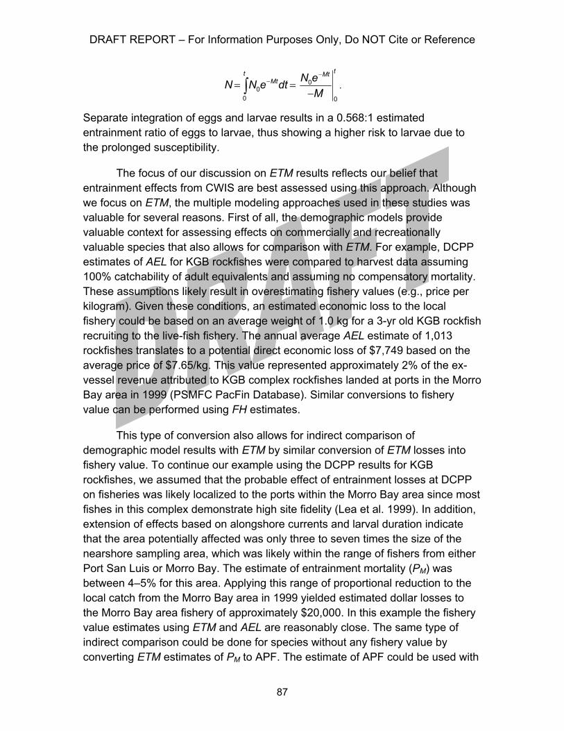
DRAFT REPORT – For Information Purposes Only, Do NOT Cite or Reference
87
00
0 0
tt MtMt N eN N e dt
M
−−= =
−∫ .
Separate integration of eggs and larvae results in a 0.568:1 estimated entrainment ratio of eggs to larvae, thus showing a higher risk to larvae due to the prolonged susceptibility.
The focus of our discussion on ETM results reflects our belief that entrainment effects from CWIS are best assessed using this approach. Although we focus on ETM, the multiple modeling approaches used in these studies was valuable for several reasons. First of all, the demographic models provide valuable context for assessing effects on commercially and recreationally valuable species that also allows for comparison with ETM. For example, DCPP estimates of AEL for KGB rockfishes were compared to harvest data assuming 100% catchability of adult equivalents and assuming no compensatory mortality. These assumptions likely result in overestimating fishery values (e.g., price per kilogram). Given these conditions, an estimated economic loss to the local fishery could be based on an average weight of 1.0 kg for a 3-yr old KGB rockfish recruiting to the live-fish fishery. The annual average AEL estimate of 1,013 rockfishes translates to a potential direct economic loss of $7,749 based on the average price of $7.65/kg. This value represented approximately 2% of the ex-vessel revenue attributed to KGB complex rockfishes landed at ports in the Morro Bay area in 1999 (PSMFC PacFin Database). Similar conversions to fishery value can be performed using FH estimates.
This type of conversion also allows for indirect comparison of demographic model results with ETM by similar conversion of ETM losses into fishery value. To continue our example using the DCPP results for KGB rockfishes, we assumed that the probable effect of entrainment losses at DCPP on fisheries was likely localized to the ports within the Morro Bay area since most fishes in this complex demonstrate high site fidelity (Lea et al. 1999). In addition, extension of effects based on alongshore currents and larval duration indicate that the area potentially affected was only three to seven times the size of the nearshore sampling area, which was likely within the range of fishers from either Port San Luis or Morro Bay. The estimate of entrainment mortality (PM) was between 4–5% for this area. Applying this range of proportional reduction to the local catch from the Morro Bay area in 1999 yielded estimated dollar losses to the Morro Bay area fishery of approximately $20,000. In this example the fishery value estimates using ETM and AEL are reasonably close. The same type of indirect comparison could be done for species without any fishery value by converting ETM estimates of PM to APF. The estimate of APF could be used with
DRAFT REPORT – For Information Purposes Only, Do NOT Cite or Reference
88
data on abundances to obtain estimates of adult populations that could be compared with demographic model results.
The demographic modeling approaches and conversions to fishery value using either demographic or ETM model results ignore any potential effects of compensation. We took this approach because there remain conflicting opinions whether larval mortality is compensated in some fashion. One side of the argument is that if compensation occurs, the estimates of FH, AEL and PM will overestimate the number of adults lost and ecosystem losses (Saila et al. 1997). The response is that it is difficult to determine if compensation occurs at all (Rose et al. 2001, Nisbet et al. 1996). Additionally, if population mortality is density independent or weakly dependent, then the recruited population size will fluctuate in response to either changes in larval abundances or mortality. In the case of large density dependent mortality, little change due to changes in recruitment might be observed in local population sizes (Cayley et al. 1996). Field experiments on west coast species of fishes have been equivocal (e.g. Stephens et al. 1986) and recent studies on boccacio (Sebastes paucispinis) showed no evidence of compensation in the stock-recruitment relationship (Tolimieri and Levin 2005). Currently, the USEPA and the California Energy Commission consider that compensation does not reduce impacts from entrainment and impingement on adult populations.
Results from demographic models are also necessary for combining estimates from entrainment and impingement unless independent data on adult fish populations are available for comparison with impingement losses. Impingement studies are designed to collect data on juveniles and adult fishes that are used to develop estimates of annual impingement. An AEL model is then used to extrapolate the number of impinged fishes either backward or forward to the numbers of adults of a certain age. By using the average age of reproductively mature females in the extrapolation these results can be combined with FH or AEL entrainment estimates to obtain estimates of the combined effects of impingement and entrainment. This approach assumes that the FH and AEL entrainment estimates are extrapolated to the same age used in the impingement estimates. Combined assessments can only be done on the few fishes with life history data available for estimating FH, AEL or one of the other demographic models. Fortunately, the total impingement losses at these three plants were relatively low due to the CWIS designs and species with the highest impingement estimates were not entrained in high abundances (Tenera Environmental 2000, 2001, 2004). This is not always the case and combining impingement and entrainment estimates into comprehensive CWIS assessments remains problematic for most species due to incomplete life history data.
DRAFT REPORT – For Information Purposes Only, Do NOT Cite or Reference
89
Another approach for combining results from impingement and entrainment would involve using the numbers of impinged individuals for a species to estimate the relative losses to the population. The impingement mortality and entrainment mortality rate estimated by ETM can be converted to survival and multiplied to estimate cumulative CWIS effects. This approach involves the assumption that there is no compensatory mechanisms acting on the population between larval and adult stages such that entrainment losses estimated by ETM represent losses to the adult population. It also assumes that impingement and entrainment losses apply to the same stock. Although this is reasonable for a closed system such as south San Diego Bay, it would be much more difficult in an open system. In addition, there are few species with adequate data on adult stocks that could be used in this approach.
Finally, demographic model results provide a direct comparison with ETM results for both fishery and non-fishery species. It is obviously preferable to present data as both percentages relative to a source population using ETM and as absolute numbers of fishes using one or both demographic models. This helps ensure that PM estimates are properly interpreted and instances where a large PM that equates to only a few adults fishes are not misinterpreted. Ensuring the species included in the assessment were adequately sampled is the best way to avoid this type of problem. Unfortunately, these types of comparison are only possible for the limited number of fishes on the west coast with published life history data. This approach is also complicated by the uncertainty related to the levels of any compensatory, depensatory, or behavioral mechanisms that may have been operating on the subject populations when the life history data were collected. The availability and uncertainty associated with life history information continue to be the greatest limitations to the use of demographic models for CWIS assessment.
Despite these limitations, the USEPA made extensive use of demographic models in the assessments used in the rule making for 316(b). This was necessary because of the need to determine the economic costs associated with implementing certain technologies that could be used to help meet performance standards for impingement (80-95%) and entrainment (60-90%) reduction mandated in the new rules. These methods will continue to be used due to the availability in the new rules of an option for site-specific compliance. This option involves a cost-benefit analysis that compares the costs of technological or operational measures for achieving the performance standards against environmental benefits calculated using benefits valuation methods provided in the new rules.

DRAFT REPORT – For Information Purposes Only, Do NOT Cite or Reference
90
4.1 GUIDELINES FOR ENTRAINMENT IMPACT ASSESSMENT The three studies presented in this paper make it clear that it is not
feasible to use a prescriptive approach to entrainment assessment design. Based on our experiences with these and other studies, we provide some general considerations that might be helpful in the design, sampling, and analysis of entrainment impact assessments. These comments are presented in the hopes that others may benefit from our experiences in conducting CWIS entrainment assessments.
Considerations for Study Design
1. Determine potential target species that could be affected by entrainment using historical data on entrainment for the power plant, if available, and data from surrounding waters. Insure that sampling will account for any endangered, threatened, or other listed species that could potentially be affected by entrainment.
2. Determine the source water areas potentially affected by entrainment including the distribution of habitats that might be differentially affected by CWIS entrainment. Different habitats may require use of different sampling gear and methods.
3. We have used oblique tows with bongo and wheeled bongo frames that sample the entire water column for both entrainment and source water because the intake structures for these plants were assumed to withdraw water from the entire water column. The locations of intakes that withdraw water from a discrete depth in the water column may require the use of pumps or closing nets for entrainment sampling at discrete water depths where water withdrawal occurs. Hydrodynamic studies should be done to verify the intake flow field for sampling at discrete depths. We have not used pumps to sample inside of power plant cooling water systems because of potential bias due to predation by biofouling organisms.
4. Determine appropriate sampling frequency based on species composition and important species that might have short spawning seasons. This could include adjusting sampling frequency seasonally based on presence of certain species. Sampling of entrainment can be done more frequently than source water sampling to provide more accurate estimates of length frequencies of entrained larvae and may also be desirable to provide more accurate estimates for calculating baseline conditions for compliance with new 316(b) rules.
5. These studies were generally conducted over a one-year period except in the case of DCPP where one of the strongest ENSO events of that century occurred during the first year of sampling. The relative effects of entrainment estimated by the ETM model should be much less subject to interannual variation than absolute estimates using FH, AEL or other

DRAFT REPORT – For Information Purposes Only, Do NOT Cite or Reference
91
demographic models. Therefore if source water sampling is done in conjunction with entrainment sampling one year is a reasonable period of sampling for these studies.
6. Use hydrodynamics of source waters to determine appropriate sampling area. In a closed system this may be the entire source water. In an open system, ocean or tidal currents should be used to determine the appropriate sampling area for estimating daily entrainment mortality (PE) for the larger source water population.
Ad hoc rule 1: Since PE is estimated as a daily mortality the sampling area should include the area potentially affected during a 24 h period. This area is a pragmatic way to arrive at a first stage estimate of daily mortality and hence survival. The use of a current meter positioned near the intake but outside the influence of its flow allows the estimation of advection in the nearby source water. The current meter approach can be combined with estimates of larval dispersion (Largier 2003) for an understanding of the magnitude of source water population affected.
Ad hoc rule 2: The PE is applied to a larger source population that is potentially affected in the time period of a larval duration. (Another option would be to use the range of the stock.) In an open system, the estimation of PM includes extrapolating the population of the sampling area to the larger source water population over a larval duration. It is difficult to say that the single current meter accurately reflects the advection of the source water population to the intake. In addition, a single current meter says very little about diffusion processes. Be sure that appropriate physical data are collected during the study to model hydrodynamics and determine size of source population.
7. The uncertainties associated with estimating larval durations, and hydrodynamics used in estimating the size of the source water populations make estimating variance for ETM problematic. One approach we have used is to base the variance calculations solely on the sampling variances used in estimating the variance of PE. A similar approach would use the CV from the source water sampling (which includes both entrainment and source water data) to estimate the variance for ETM or use a Monte Carlo approach using the upper and lower confidence limit values for the PE values. These approaches have been considered because of the large unrealistic error terms derived using the Delta method that incorporates all of the multiple intercorrelated sources of error in the model.
Considerations for Sampling and Processing
1. We have used sample volumes of 30-60 m3 per sample for these and other studies but this volume should be adjusted for the larval

DRAFT REPORT – For Information Purposes Only, Do NOT Cite or Reference
92
concentrations in the source waters. The appropriate sample volume is best determined by preliminary sampling using the gear proposed for the study.
2. Be sure that mesh size used for net sampling is appropriate for potential target species. We have used 335 µm mesh nets because we have observed fish larvae being extruded through 505 µm mesh nets. Much smaller sized mesh would be needed to sample invertebrate larvae effectively.
3. Although we generally combine the subsamples from the two bongo nets for analysis, preserving one of them directly in 70-80% ethanol allows for genetic analyses to be conducted and analysis of otoliths to determine age and growth rates. Larval fishes are generally easier to identify when initially preserved in 5-10% formalin.
4. If ageing using larval otoliths is not done, be sure that length frequencies measured from entrainment samples are realistic based on available life history. We applied general rules for using the length data for determining mean, minimum, and maximum ages, but would recommend developing criteria based on the length frequency distribution for each species.
5. Be sure to account for egg stages that would be subject to entrainment if fish eggs are not sorted and identified from the samples.
Considerations for Analysis
1. Use multiple modeling approaches to validate results and provide additional data for determining effects at the adult population level.
2. Similar to the approach of using multiple models to provide additional data for determining effects at the adult population level, the ETM results can be converted into another currency using APF. This approach is probably most appropriate for scaling restoration projects that could be used to help offset losses due to entrainment.
3. Although FH and AEL models can be hindcast or extrapolated to the same age they will not necessarily provide the same estimate unless the data used in the two models are derived from a life table assuming a stable age distribution.
4. FH and AEL are estimates of the number of adults at a specific age. To estimate the number of adult females in the population, NF, the average fecundity can be used instead of TLF. The AEL analog is extrapolation to all adult fish ages - AEL'. A comparison can be made using the relation AEL'=2NF. This age of entry into the adult population may need to be adjusted to the average age of fishery catch if comparisons are being made with fishery data. The use of AEL and FH (Horst 1975 and Goodyear 1978), aligning at fishery age, is one method of estimating losses in terms of adult animals.

DRAFT REPORT – For Information Purposes Only, Do NOT Cite or Reference
93
5. Another estimate would use production foregone or total biomass that would have been produced by entrained or impinged animals, had they not been entrained or impinged (Rago 1984). Production foregone includes all biomass lost through all forms of mortality had the animals survived entrainment or impingement. This measure is most often used for forage species and represents ecosystem losses, e.g. to other trophic levels. Age-1 equivalent loss is a measure similar to AEL and FH that is most commonly used for harvested species. The USEPA (2002) used age-1 equivalents to evaluate power plant losses “because methods are unavailable for valuing fish eggs and larvae.” They conservatively estimated fish landings value using the number of age-1 individuals, as the average fishery age is older in most cases. However the USEPA believed the method may underestimate the true value of reducing impingement and entrainment because life history data were not available for most species. If survival rates from the age of entrainment until adulthood are accurate, FH and AEL underestimate the numbers of lost adults because they are extrapolated to a single age, e.g. age of maturity in the case of FH. An improved approach to FH will be to use the average annual fecundity to estimate the equivalent number of females NF removed from the standing stock of adults. Similarly, AEL can be extrapolated to all adult ages and summed to estimate the number of adult equivalents AEL' and these measures can then be compared with fishery losses. However, the accuracy of these kinds of estimates is subject to the accuracy of the underlying survival and fecundity estimates.
6. Another estimate of the number of equivalent adults lost by larval entrainment is to use the mortality estimate from the ETM procedure and apply it to a survey of the standing stock. This accuracy of this estimate is subject to the accuracy of the estimate of the source population affected. This method may result in improvements when there is little confidence in survival estimates or when there is conjecture about compensatory processes that may negate the underlying models of AEL and FH.
4.2 CONCLUSION As should be clear from this report, we feel that CWIS impacts are best
evaluated using empirically based source water body information and the ETM model, and not using demographic models based on life history information derived from various sources with varying, or unknown, levels of confidence. There is no reason to use demographic modeling approaches for assessing CWIS impacts with the availability of approaches such as the ETM that provide estimates based on empirically derived estimates. In contrast to demographic models, uncertainty associated with ETM model estimates can be controlled through changes to the sampling design for the entrainment and source water sampling. The CEC and CCC have all required the ETM approach in recent

DRAFT REPORT – For Information Purposes Only, Do NOT Cite or Reference
94
studies. Hopefully the information in this paper will assist others in the design and analysis of CWIS assessments that meet the requirements of both 316(b) and regulatory requirements of other agencies.

DRAFT REPORT – For Information Purposes Only, Do NOT Cite or Reference
95
ACKNOWLEDGEMENTS
It should be obvious that large studies like these require the coordinated work of many people. We would first like to thank the California Energy Commission, especially Rick York and Dick Anderson for funding this study and recognizing the importance of publishing this work so it could be used by other researchers and decision makers. Thanks also to Duke Energy and Pacific Gas and Electric Company (PG&E) for the use of the data from the Duke Energy South Bay and Morro Bay Power Plants and the PG&E Diablo Canyon Power Plant. Special thanks go to James White and Brian Waters from Duke Energy, and Kathy Jones, Anne Jackson, Jim Kelly, and Bryan Cunningham from PG&E. We also want to thank Michael Thomas from the Central Coast Regional Water Quality Control Board who organized the Technical Workgroup that provided input on the Diablo Canyon and Morro Bay studies which provided a model of cooperative science used in other studies throughout the state. More special thanks go to the Technical Workgroup members from various state and federal resource agencies and academia who provided valuable input on all three studies. Dr. John Skalski helped develop the models used in the assessments and Drs. Roger Nisbet, Allen Stewart-Oaten, Alec MacCall and others provided valuable input on various aspects of the studies. We want to thank Chris Ehrler and Jay Carroll from Tenera Environmental, and Rick York and Joanna Grebel from the California Energy Commission for their editorial assistance with the report. Finally we want to thank all of the scientists and technicians at Tenera Environmental who collected all of these data and processed the hundreds of samples collected from the three studies.
DRAFT REPORT – For Information Purposes Only, Do NOT Cite or Reference
96
LITERATURE CITED
Allen, L. G., R. E. Jensen, and J. R. Sears. 1990. Open coast settlement and distribution of young-of-the-year California halibut (Paralichthys californicus) along the southern California coast between Point Conception and San Mateo Point, June-October, 1988. Calif. Dep. Fish Game, Fish. Bull. 174:145−152.
Allen, L. G. 1999. Fisheries Inventory and Utilization of San Diego Bay, San Diego, California. Final Report: Sampling Period July 1994 to April 1999. Prepared for the U.S. Navy and the San Diego Unified Port District.
Barlow, G.W. 1963. Species structure of the Gobiid fish Gillichthys mirabilis from coastal sloughs of the eastern Pacific. Pac. Sci. XVII(1):47−72.
Barnthouse, L. W. 2000. Impacts of power-plant cooling systems on estuarine fish populations: The Hudson River after 25 years. In Environmental Science & Policy, Power Plants & Aquatic Resources: Issues and Assessment (Wisniewski, J., ed.)., Vol. 3, Sup. 1. p. S341−S348. Elsevier Science Ltd., NY.
Barnthouse, L. W., R. J. Klauda, D. S. Vaughan, and R. L. Kendall. 1988. Science, Law, and Hudson River Power Plants: A case study in environmental impact assessment. Amer. Fish. Soc. Spec. Monogr. 4, 346 p.
Baruskov, V. V. 1981. A brief review of the subfamily Sebastinae. J. Ichthy. 21:1−26.
Behrens, D. W., D. C. Sommerville. 1982. Impingement studies at the Morro Bay Power Plant. Report 026.22-80.1. Pacific Gas and Electric Company, Dept. Eng. Res., San Ramon, CA.
Boreman, J., C. P. Goodyear, and S. W. Christensen. 1978. An empirical transport model for evaluating entrainment of aquatic organism by power plants. US Fish Wildl. Ser. FWS/OBS-78/90, Ann Arbor, MI.
Boreman, J., C. P. Goodyear, and S. W. Christensen. 1981. An empirical methodology for estimating entrainment losses at power plants sited on estuaries. Trans. Am. Fish. Soc. 110:253−260.
Brothers, E. B. 1975. The comparative ecology and behavior of three sympatric California gobies. Ph.D. Thesis, Univ. Calif., San Diego, CA.
DRAFT REPORT – For Information Purposes Only, Do NOT Cite or Reference
97
Bulleit, K. A. N. 2000. Achieving sustainable development: A review of the environmental balancing act in two key clean water act regulatory programs. In Environmental Science & Policy; Power Plants & Aquatic Resources: Issues and Assessment (Wisniewski, J., ed.), Vol. 3, Supplement 1. Elsevier Science Ltd., NY, 512 p.
Burge, R. T., and S. A. Schultz. 1973. The marine environment in the vicinity of Diablo Cove, with special reference to abalones and bony fishes. Mar. Res. Tech. Rep. No. 19.
Cayley, M. J., M. H. Carr, M. A. Hixon, T. P. Hughes, G. P. Jones, and B. A. Menge. 1996. Recruitment and the local dynamics of open marine populations. Ann. Rev. Ecol. Syst. 27:477−500.
DeLacy, A. C., C. R. Hitz, and R. L. Dryfoos. 1964. Maturation, gestation, and birth of rockfish (Sebastodes) from Washington and adjacent waters. Fish. Res. Papers. Wash. Dep. Fish. 2(3):51−67.
Dey, W. P. 2003. Use of equivalent loss models under Section 316(b) of the Clean Water Act. In Defining and assessing adverse environmental impact from power plant impingement and entrainment of aquatic organism (D. A. Dixon, J. A. Veil, and J. Wisniewski, eds.), p. 247−263. A. A. Balkema Publishers, Netherlands.
Ehrler, C. P., J. R. Steinbeck, E. A. Laman, J. B. Hedgepeth, J. R. Skalski, and D. L. Mayer. 2003. A process for evaluating adverse environmental impacts by cooling-water system entrainment at a California power plant. In Defining and assessing adverse environmental impact from power plant impingement and entrainment of aquatic organism (D. A. Dixon, J. A. Veil, and J. Wisniewski, eds.). p. 79−102. A. A. Balkema Publishers, Netherlands.
Englert, T. L., and J. Boreman. 1988. Historical review of entrainment impact estimates and the factors influencing them. Am. Fish. Soc. Spec. Monogr. 4:143−151.
Goodyear, C. P. 1978. Entrainment impact estimates using the equivalent adult approach. United States Fish and Wildlife Service, FWS/OBS-78/65, Ann Arbor, MI.
Horst, T. J. 1975. The assessment of impact due to entrainment of ichthyoplankton. In Fisheries and Energy Production: A symposium (S. B. Saila, ed.). p. 107−118. Lexington Books, D.C. Heath and Company, Lexington, MA.
DRAFT REPORT – For Information Purposes Only, Do NOT Cite or Reference
98
Kendall, A. W. Jr., and W. H. Lenarz. 1987. Status of early life history studies of northeast Pacific rockfishes. In Proceedings of the International Rockfish Symposium. p. 99−128. Univ. Alaska SeaGrant Rep. 87-2.
Laidig, T. E., K. M. Sakuma, and M. M. Nishimoto. 1995. Description of pelagic larval and juvenile stripetail rockfish, Sebastes saxicola (family Scorpaenidae), with an examination of larval growth. Fish. Bull. 94:289−299.
Largier, J. L. 1995. San Diego Bay circulation: a study of the circulation of water in San Diego Bay for the purpose of assessing, monitoring and managing the transport and potential accumulation of pollutants and sediment in San Diego Bay. Scripps Inst. Oceanogr. Tech. Rep. #1-188-190-0. Final Report prepared for Calif. State Water Res. Control Board and the Calif. Reg. Water Quality Control Board, San Diego Region.
Largier, J. L., C. J. Hearn, and D. B. Chadwick. 1996. Density structures in low inflow estuaries. In Buoyancy Effects on Coastal Estuarine Dynamics Coastal Estuarine Studies (D. G. Aubrey and C. T. Friedrichs, eds.). p. 227-242. Am. Geophys. Union, Vol. 53, Washington, D.C.
Largier, J. L. 2003. Considerations in estimating larval dispersal distances from oceanographic data. Ecol. App. 13(1) Sup 71−89.
Lea, R. N., R. D. McAllister, and D. A. VenTresca. 1999. Biological aspects of nearshore rockfishes of the genus Sebastes from central California. Calif. Dep. Fish Game Fish. Bull. 177, 107 p.
Love, M. S., and K. Johnson. 1999. Aspects of the life histories of grass rockfish, Sebastes rastrelliger, and brown rockfish, S. auriculatus, from southern California. Fish. Bull. 97(1):100−109.
Lynn, R. J., T. Baumgartner, J. Garcia, C. A. Collins, T. L. Hayward, K. D. Hyrenbach, A. W. Mantyla, T. Murphree, A. Shankle, F. B. Schwing, K. M. Sakuma, and M. J. Tegner. 1998. The state of the California Current, 1997–1998: Transition to El Niño conditions. Calif. Coop. Oceanic Fish. Invest. Rep. 39:25−51.
MacCall, A. D., K. R. Parker, R. Leithiser, and B. Jessee. 1983. Power plant impact assessment: A simple fishery production model approach. Fish. Bull. 81(3): 613−619.
MacGregor, J. S. 1970. Fecundity, multiple spawning and description of gonads in Sebastodes. U.S. Fish and Wildlife Serv. Spec. Sci. Rep., no. 596, 12 p.
DRAFT REPORT – For Information Purposes Only, Do NOT Cite or Reference
99
MBC Applied Environmental Sciences and Tenera Environmental. 2005. AES Huntington Beach L.L.C. Generating Station entrainment and impingement study: final report. Prepared for AES Huntington Beach L.L.C. and the California Energy Commission. April 2005, 224 p.
Mayhew, D. A., L. D. Jensen, D. F. Hanson, and P. H. Muessig. 2000. A comparative review of entrainment survival studies at power plants in estuarine environments. In Environmental Science & Policy; Power Plants & Aquatic Resources: Issues and Assessment (J. Wisniewski ed.), Vol. 3, Supplement 1, p. S295−S302. Elsevier Science Ltd., NY.
Miller, D. J., and R. N Lea. 1972. Guide to the Coastal Marine Fishes of California. Calif. Dep. Fish Game Fish Bull. 157. Sacramento, CA, 249 p.
Moreno, G. 1993. Description of early larvae of four northern California species of rockfishes (Scorpaenidae: Sebastes) from rearing studies. NOAA Tech. Rept. NMFS 116, 18 p.
Moser, H. G. 1996. The early stages of fishes in the California current region. Calif. Coop. Oceanic Fish. Invest., Atlas No. 33; 1214−1226. Allen Press Inc., Lawrence, KS.
Moser, H. G., E. H. Ahlstrom, and E. M. Sandknop. 1977. Guide to the identification of scorpionfish larvae (family Scorpaenidae) in the eastern Pacific with comparative notes on species of Sebastes and Helicolenus from other oceans. NOAA Tech. Rept. NMFS Circ. 402, 71 p.
Moser, H. G. and E. H. Ahlstrom. 1978. Larvae and pelagic juveniles of blackgill rockfish, Sebastes melanostomus, taken in midwater trawls off southern California and Baja California. J. Fish. Res. Board Can. 35(7):981−996.
Nagle, D. G., and J. T. Morgan, Jr. 2000. A draft regulatory framework for analyzing potential adverse environmental impact from cooling water intake structures. In Environmental Science & Policy; Power Plants & Aquatic Resources: Issues and Assessment (J. Wisniewski, ed.), p. IX-XIV. Vol. 3, Sup. 1. Elsevier Science Ltd., NY.
Nisbet, R. M., W. Murdoch and A. Stewart-Oaten. 1996. Consequences for adult fish stocks of human-induced mortality on immatures. In: Detecting ecological impacts: Concepts and applications in coastal habitats (R. J Schmitt and C. W. Osenberg, eds.), p. 257−277. Academic Press, San Diego, CA.
Nishimoto, M. M. In prep. Identification of Sebastes larvae.

DRAFT REPORT – For Information Purposes Only, Do NOT Cite or Reference
100
NOAA. 1999. El Niño-Southern Oscillation (ENSO) (http://www.ogp.noaa.gov/enso/).
Public Service Electric and Gas Company (PSE&G). 1993. Appendix I—Modeling. Permit No. NJ0005622. Prepared by Lawler, Matusky, and Skelly Engineers, Pearl River, NY. Comments on NJPDES Draft, 82 p.
Parker, K. R. 1980. A direct method for estimating northern anchovy, Engraulis mordax, spawning biomass. Fish. Bull. 78:541−544.
Parker, K. R. 1985. Biomass model for the egg production method. In An egg production method for estimating spawning biomass of pelagic fish: Application to the northern anchovy, Engraulis mordax. (R. Lasker, ed.), p. 5-6. U.S. Dep. Comm., NOAA Tech. Report NMFS 36.
Parker, K. R., and E. E. DeMartini. 1989. Chapter D: Adult-equivalent loss. Technical Report to the California Coastal Commission. Prepared by Marine Review Committee, Inc., 56 p.
Parrish, R. H., Serra, R. and W. S. Grant 1989. The monotypic sardine, Sardina and Sardinops: their taxonomy, distribution, stock structure, and zoogeography. Can. J. Fish. Aquat. Sci. 2019−2036.
Rago, P. J. 1984. Production forgone: An alternative method for assessing the consequences of fish entrainment and impingement losses at power plants and other water intakes. Ecol. Model. 24:789−111
Rose, K. A., J. H. Cowan, K. O. Winemiller, R. A. Myers, and R. Hilborn. 2001. Compensatory density dependence in fish populations: importance, controversy, understanding, and prognosis. Fish and Fisheries 2:293−327.
Ricker, W. E. 1975. Computation and interpretation of biological statistics of fish populations. Fish. Res. Board Can. Bull. 91, 382 p.
Saila, S. B., X. Chen. K. Erzini, and B. Martin. 1987. Compensatory mechanisms in fish populations: Literature reviews. Vol. 1: Critical evaluation of case histories of fish populations experiencing chronic exploitation or impact. EA-5200. Report prepared for the Electric Power Research Institute.
Seber, G. A. F. 1982. The estimation of animal abundance and related parameters. McMillan, London. 654 p.
Smith, P. E., and S. L. Richardson. 1977. Standard techniques for pelagic fish egg and larva surveys. FAO Fish. Tech. Paper 175:1−100.

DRAFT REPORT – For Information Purposes Only, Do NOT Cite or Reference
101
Tenera Environmental. 1997. Diablo Canyon Power Plant 316(b) demonstration study: Phase 1: Entrainment study design, Part II: Selection of target organisms, sampling methods, and gear testing. Prepared for Pacific Gas & Electric Co., San Francisco, CA.
Tenera Environmental. 2000. Diablo Canyon Power Plant: 316(b) demonstration report. Prepared for Pacific Gas and Electric Co., San Francisco, CA.
Tenera Environmental. 2001. Morro Bay Power Plant modernization project 316(b) resource assessment. Prepared for Duke Energy Morro Bay, LLC, Morro Bay, CA.
Tenera Environmental. 2004. South Bay Power Plant cooling water system effects on San Diego Bay; Volume II: Compliance with Section 316(b) of the Clean Water Act for the South Bay Power Plant. Prepared for Duke Energy South Bay, Chula Vista, CA.
Theilacker, G. H. 1980. Changes in body measurements of larval northern anchovy, Engraulis mordax, and other fishes due to handling and preservation. Fish. Bull. 78:685−692.
Tolimieri, N., and P. S. Levin. 2005. The roles of fishing and climate in the population dynamics of boccacio rockfish. Ecol. App. 15:458−468.
U.S. Environmental Protection Agency (USEPA). 1977. Guidance for evaluating the adverse impact of cooling water intake structures on the aquatic environment: Section 316(b) P.L. 92-500, 58 p.
USEPA. 2002. Case study analysis for the proposed Section 316(b) Phase II existing facilities rule. EPA-821-R-02-002.
USEPA. 2004. National Pollutant Discharge Elimination System: Final regulations to establish requirements for cooling water intake structures at Phase II existing facilities; Final Rule, 40 CFR Parts 9, 122 et al. Published in Federal Register, Vol. 69:41575−41693, July 9, 2004.
Veil, J. A. 2000. Potential impacts of 316(b) regulatory controls on economics, electricity reliability, and the environment. In Environmental Science & Policy. Power Plants & Aquatic Resources: Issues and Assessment, (J. Wisniewski, ed.). Vol. 3, Sup. 1 pp S1−S6. Elsevier Science Ltd., NY, 512 p.
Veil, J. A., M. G. Puder, D. J. Littleton, and N. Johnson. 2003. A holistic look at minimizing adverse environmental impact under Section 316(b) of the Clean Water Act. In Defining and assessing adverse environmental impact from
DRAFT REPORT – For Information Purposes Only, Do NOT Cite or Reference
102
power plant impingement and entrainment of aquatic organism (D. A. Dixon, J. A. Veil, and J. Wisniewski, eds.). p. 40–55. A.A. Balkema Publishers, Netherlands, 291 pp.
Wang, J. C. S. 1986. Fishes of the Sacramento-San Joaquin estuary and adjacent waters, California: A guide to the early life stages. Tech. Rep. 9, January 1986.
Wilson, C. D., and G. W. Boehlert. 1990. The effects of different otolith ageing techniques on estimates of growth and mortality for the splitnose rockfish, Sebastes diploproa, and canary rockfish, S. pinniger. Calif. Dep. Fish Game 76(3):146−160.
Wyllie Echeverria, T. 1987. Thirty-four species of California rockfishes: maturity and seasonality of reproduction. Fish. Bull. 85(2):229−250.
Yoklavich, M. M., V. J. Loeb, M. Nishimoto, and B. Daly. 1996. Nearshore assemblages of larval rockfishes and their physical environment off central California during an extended El Niño event, 1991−1993. Fish. Bull. 94:766−782.
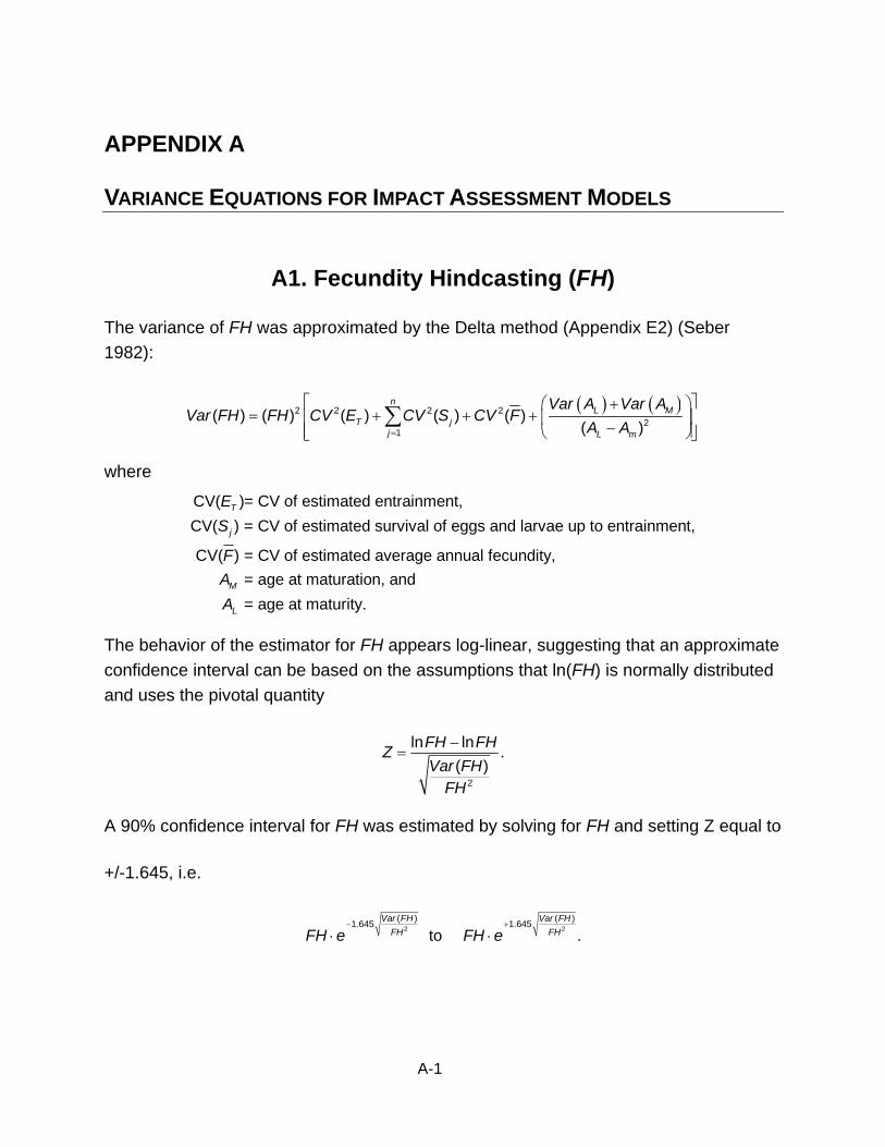
A-1
APPENDIX A VARIANCE EQUATIONS FOR IMPACT ASSESSMENT MODELS
A1. Fecundity Hindcasting (FH)
The variance of FH was approximated by the Delta method (Appendix E2) (Seber 1982):
( ) ( )2 2 2 22
1( ) ( ) ( ) ( ) ( )
( )
nL M
T jj L m
Var A Var AVar FH FH CV E CV S CV F
A A=
⎡ ⎤⎛ ⎞+= + + +⎢ ⎥⎜ ⎟−⎢ ⎥⎝ ⎠⎣ ⎦
∑
where
CV( )= CV of estimated entrainment,CV( ) = CV of estimated survival of eggs and larvae up to entrainment,
CV( ) = CV of estimated average annual fecundity, = age at maturation, and = age at matur
T
j
M
L
ES
FAA ity.
The behavior of the estimator for FH appears log-linear, suggesting that an approximate confidence interval can be based on the assumptions that ln(FH) is normally distributed and uses the pivotal quantity
2
ln ln .( )
FH FHZVar FH
FH
−=
A 90% confidence interval for FH was estimated by solving for FH and setting Z equal to
+/-1.645, i.e.
2 2( ) ( )1.645 1.645
to .Var FH Var FH
FH FHFH e FH e− +
⋅ ⋅

A-2
A2. Adult Equivalent Loss (AEL)
The AEL approach uses estimates of the abundance of entrained or impinged organisms to forecast the loss of equivalent numbers of adults. Starting with the number of age class j larvae entrained (Ej), it is conceptually easy to convert these numbers to an equivalent number of adults lost (AEL) at some specified age class from the formula:
1
n
j jj
AEL E S=
= ∑ ,
where
j
j
number of age classes,E = estimated number of larvae lost in age class j, and
S = survival rate for the jth age class to adulthood (Goodyear 1978).
n =
Age-specific survival rates from larval stage to recruitment into the fishery (through juvenile and early adult stages) must be included in this assessment method. For some commercial species, survival rates are known for adults in the fishery; but for most species, age-specific larval survivorship has not been well described.
Survivorship to recruitment, to an adult age, was apportioned into several age stages, and AEL was calculated using the total entrainment as
1
n
T jj
AEL E S=
= ∏ ,
where
j
number of age classes from entrainment to recruitment andS = survival rate from the beginning to end of the jth age class. n =
The variance of AEL can be estimated using a Taylor series approximation (Delta method of Seber 1982) as
2 2 2
1( ) ( ) ( )
n
T jj
Var AEL AEL CV E CV S=
⎛ ⎞= +⎜ ⎟
⎝ ⎠∑ .

A-3
A3. Proportional Entrainment and ETM
The Empirical Transport Model (ETM) calculations provide an estimate of the probability of mortality due to power plant entrainment. The values used in calculating proportional entrainment (PE) are population estimates based on the respective larval densities and volumes of the cooling water system flow and source water areas. On any one sampling day, the conditional entrainment mortality can be expressed as
( )
i
i
abundance of entrained larvaeabundance of larvae in source populationprobability of entrainment in th time period 1, , .
iPE
i i N
=
= = …
In turn, the daily probability can be estimated and expressed as
ii
i
EPER
=
where Ei = estimated abundance of larvae entrained in the ith time period
( )1, ,i N= … ;
Ri = estimated abundance of larvae at risk of entrainment from the source population in the ith time period ( )1, ,i N= … .
The variance for the period estimate of PE can be expressed as
( ) ,ii i i
i
EVar PE Var E RR
⎛ ⎞= ⎜ ⎟⎜ ⎟
⎝ ⎠.
Assuming zero covariance between the entrainment and source and using the delta method (Seber 1982), the variance of an estimator formed from a quotient (like PEi) can be effectively approximated by
2 2
( ) ( ) .
A AA B BVar Var A Var BB A B
⎛ ⎞ ⎛ ⎞⎡ ⎤ ⎡ ⎤∂ ∂⎜ ⎟ ⎜ ⎟⎢ ⎥ ⎢ ⎥⎛ ⎞ ⎣ ⎦ ⎣ ⎦⎜ ⎟ ⎜ ⎟≈ +⎜ ⎟ ∂ ∂⎜ ⎟ ⎜ ⎟⎝ ⎠⎜ ⎟ ⎜ ⎟⎝ ⎠ ⎝ ⎠
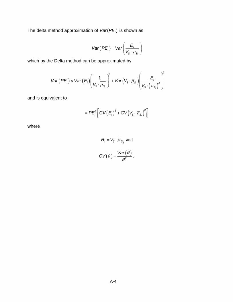
A-4
The delta method approximation of ( )iVar PE is shown as
( ) ii
S Si
EVar PE VarV ρ⎛ ⎞
= ⎜ ⎟⋅⎝ ⎠
which by the Delta method can be approximated by
( ) ( ) ( )( )
22
21
i
i i
ii i S S
S S S S
EVar PE Var E Var VV V
ρρ ρ
⎛ ⎞⎛ ⎞ −⎜ ⎟≈ + ⋅⎜ ⎟⎜ ⎟ ⎜ ⎟⋅ ⋅⎝ ⎠ ⎝ ⎠
and is equivalent to
( ) ( )222ii i S SPE CV E CV V ρ⎡ ⎤= + ⋅⎢ ⎥⎣ ⎦
where
Si S ijR V ρ= ⋅ and
( ) ( )2 .
VarCV
θθ
θ=
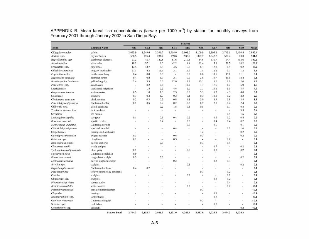
A-5
APPENDIX B. Mean larval fish concentrations (larvae per 1000 m3) by station for monthly surveys from February 2001 through January 2002 in San Diego Bay.
StationsTaxon Common Name SB1 SB2 SB3 SB4 SB5 SB6 SB7 SB8 SB9 Mean
CIQ goby complex gobies 2,095.9 1,549.6 2,391.7 2,914.0 3,003.0 4,109.9 3,995.8 2,743.1 2,400.4 2,800.4Anchoa spp. bay anchovies 556.5 476.4 231.4 159.6 938.9 1,327.7 1,042.7 520.4 73.3 591.9Hypsoblennius spp. combtooth blennies 27.2 45.7 140.8 81.6 210.8 84.6 575.7 94.4 453.6 190.5Atherinopsidae silversides 18.2 57.1 6.0 42.2 11.4 22.4 5.3 58.5 18.2 26.6Syngnathus spp. pipefishes 12.5 13.7 8.3 4.5 16.0 8.1 12.8 6.9 9.2 10.2Gillichthys mirabilis longjaw mudsucker 27.1 4.3 11.5 3.1 15.9 1.5 12.2 0.7 1.2 8.6Engraulis mordax northern anchovy 0.4 0.8 0.9 - 6.9 0.8 18.6 15.1 11.1 6.1Hypsopsetta guttulata diamond turbot 0.4 0.8 1.9 2.1 5.9 2.6 10.7 11.8 18.4 6.1Acanthogobius flavimanus yellowfin goby 2.4 3.5 0.6 12.0 2.9 15.1 1.0 1.9 2.0 4.6Paralabrax spp. sand basses - 0.2 0.6 - 12.2 1.1 17.6 1.7 6.9 4.5Labrisomidae labrisomid kelpfishes - 1.4 2.5 4.8 2.0 1.1 10.1 9.0 5.5 4.0Genyonemus lineatus white croaker 0.5 1.0 1.8 2.3 6.3 5.3 6.7 4.3 4.8 3.7Sciaenidae croakers 0.7 0.4 1.0 0.2 5.1 0.3 10.1 0.2 4.2 2.5Cheilotrema saturnum black croaker 0.2 0.3 0.5 0.8 4.1 3.0 3.9 0.8 3.8 1.9Paralichthys californicus California halibut 0.1 0.5 0.2 0.2 0.5 0.7 2.0 0.4 2.4 0.8Gibbonsia spp. clinid kelpfishes - - 0.2 1.8 0.8 0.5 - 0.7 0.8 0.5Trachurus symmetricus jack mackerel - - - - - - - - 3.5 0.4Serranidae sea basses - - - - - - - 0.9 1.5 0.3Lepidogobius lepidus bay goby 0.1 - 0.3 0.4 0.2 - 0.5 0.2 0.4 0.2Roncador stearnsi spotfin croaker - - 0.4 - 0.6 - 0.4 0.4 0.2 0.2Menticirrhus undulatus California corbina - - - - 0.9 - 0.5 - 0.1 0.2Citharichthys stigmaeus speckled sanddab - - - 0.4 - - - 0.2 1.0 0.2Clupeiformes herrings and anchovies - - - - - 1.2 - - 0.2 0.2Odontopyxis trispinosa pygmy poacher 0.3 - - 0.6 - 0.3 - - 0.2 0.2Gobiesox spp. clingfishes 0.2 - - 0.3 - - - 0.6 - 0.1Hippocampus ingens Pacific seahorse - - 0.3 - - 0.3 - 0.4 - 0.1Clinocottus analis wooly sculpin - - - - - - 0.7 - 0.2 0.1Typhlogobius californiensis blind goby 0.1 - - - 0.3 - 0.3 - 0.2 0.1Strongylura exilis California needlefish 0.9 - - - - - - - - 0.1Ruscarius creaseri roughcheek sculpin 0.3 - 0.3 - - - - - 0.2 0.1Leptocottus armatus Pacific staghorn sculpin - - - 0.2 - - 0.3 0.3 - 0.1Artedius spp. sculpins - - - - 0.3 - - - 0.2 0.1Hyporhamphus rosae California halfbeak 0.4 0.2 - - - - - - - 0.1Paralichthyidae lefteye flounders & sanddabs - - - - - 0.3 - 0.2 - 0.1Cottidae sculpins - - - - 0.2 - - 0.2 - 0.1Oligocottus spp. sculpins - - - - - - 0.2 0.2 - 0.1Pleuronichthys ritteri spotted turbot - - - - - - - 0.4 - 0.1Atractoscion nobilis white seabass - - - - 0.2 - - 0.2 - <0.1Porichthys myriaster specklefin midshipman - - - - - 0.3 - - - <0.1Clupeidae herrings - - - - - - 0.3 - - <0.1Nannobrachium spp. lanternfishes - - - - - - 0.2 - - <0.1Gobiesox rhessodon California clingfish - - - - - 0.2 - - - <0.1Sebastes spp. rockfishes - - - - - - 0.2 - - <0.1Citharichthys spp. sanddabs - - - - - - - - 0.2 <0.1
Station Total 2,744.3 2,155.7 2,801.3 3,231.0 4,245.4 5,587.0 5,728.8 3,474.2 3,024.3
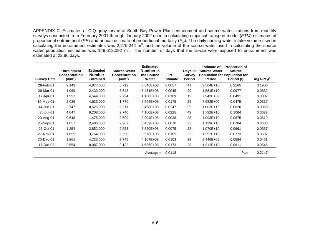
A-6
APPENDIX C. Estimates of CIQ goby larvae at South Bay Power Plant entrainment and source water stations from monthly surveys conducted from February 2001 through January 2002 used in calculating empirical transport model (ETM) estimates of proportional entrainment (PE) and annual estimate of proportional mortality (PM). The daily cooling water intake volume used in calculating the entrainment estimates was 2,275,244 m3, and the volume of the source water used in calculating the source water population estimates was 149,612,092 m3. The number of days that the larvae were exposed to entrainment was estimated at 22.86 days.
Survey Date
Entrainment Concentration
(#/m3)
Estimated Number Entrained
Source Water Concentration
(#/m3)
Estimated Number in the Source
Water PE
Estimate
Days in Survey Period
Estimate of Source Water Population for
Period
Proportion of Source
Population for Period (f) =fi(1-PEi)d
28-Feb-01 2.143 4,877,000 5.712 8.546E+08 0.0057 41 3.504E+10 0.2165 0.1900 29-Mar-01 1.069 2,433,000 3.643 5.451E+08 0.0045 29 1.581E+10 0.0977 0.0882 17-Apr-01 1.997 4,544,000 2.794 4.180E+08 0.0109 19 7.942E+09 0.0491 0.0382
16-May-01 2.036 4,633,000 1.770 2.649E+08 0.0175 29 7.682E+09 0.0475 0.0317 14-Jun-01 3.747 8,525,000 2.311 3.458E+08 0.0247 29 1.003E+10 0.0620 0.0350 26-Jul-01 4.047 9,208,000 2.740 4.100E+08 0.0225 42 1.722E+10 0.1064 0.0633
23-Aug-01 0.648 1,475,000 2.609 3.904E+08 0.0038 28 1.093E+10 0.0675 0.0619 25-Sep-01 1.057 2,406,000 2.307 3.452E+08 0.0070 33 1.139E+10 0.0704 0.0600 23-Oct-01 1.254 2,852,000 2.553 3.820E+08 0.0075 28 1.070E+10 0.0661 0.0557 27-Nov-01 1.655 3,764,000 2.390 3.576E+08 0.0105 35 1.252E+10 0.0773 0.0607 20-Dec-01 1.861 4,233,000 2.745 4.107E+08 0.0103 23 9.446E+09 0.0584 0.0461 17-Jan-02 3.554 8,087,000 3.132 4.686E+08 0.0173 28 1.312E+10 0.0811 0.0545
Average = 0.0118 PM= 0.2147
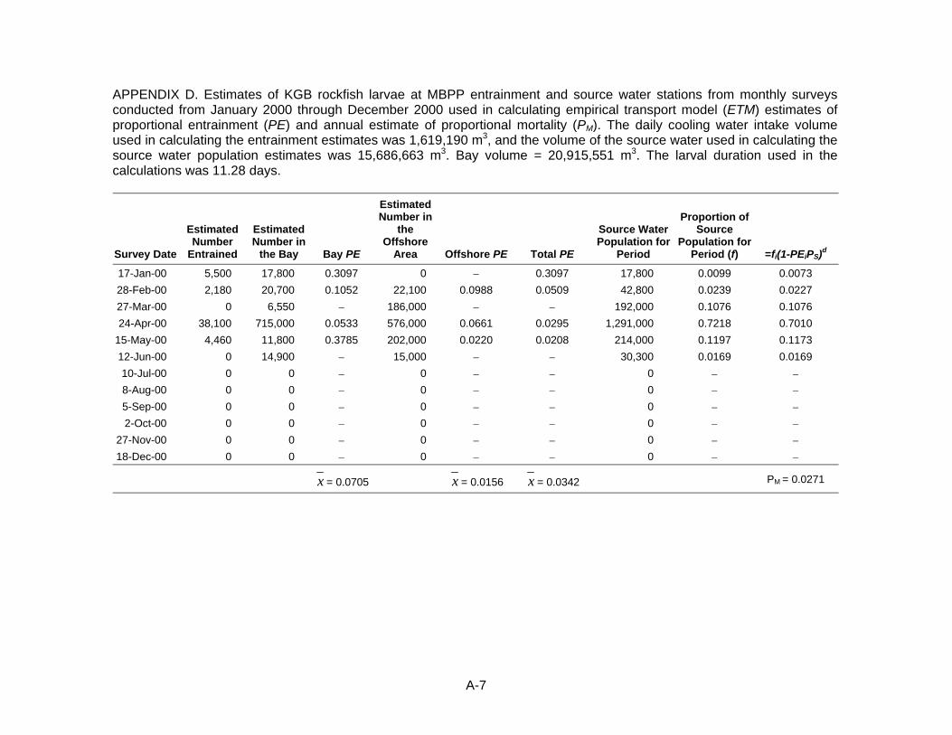
A-7
APPENDIX D. Estimates of KGB rockfish larvae at MBPP entrainment and source water stations from monthly surveys conducted from January 2000 through December 2000 used in calculating empirical transport model (ETM) estimates of proportional entrainment (PE) and annual estimate of proportional mortality (PM). The daily cooling water intake volume used in calculating the entrainment estimates was 1,619,190 m3, and the volume of the source water used in calculating the source water population estimates was 15,686,663 m3. Bay volume = 20,915,551 m3. The larval duration used in the calculations was 11.28 days.
Survey Date
Estimated Number
Entrained
Estimated Number in
the Bay Bay PE
Estimated Number in
the Offshore
Area Offshore PE Total PE
Source Water Population for
Period
Proportion of Source
Population for Period (f) =fi(1-PEiPS)d
17-Jan-00 5,500 17,800 0.3097 0 − 0.3097 17,800 0.0099 0.0073 28-Feb-00 2,180 20,700 0.1052 22,100 0.0988 0.0509 42,800 0.0239 0.0227 27-Mar-00 0 6,550 − 186,000 − − 192,000 0.1076 0.1076 24-Apr-00 38,100 715,000 0.0533 576,000 0.0661 0.0295 1,291,000 0.7218 0.7010
15-May-00 4,460 11,800 0.3785 202,000 0.0220 0.0208 214,000 0.1197 0.1173 12-Jun-00 0 14,900 − 15,000 − − 30,300 0.0169 0.0169 10-Jul-00 0 0 − 0 − − 0 − − 8-Aug-00 0 0 − 0 − − 0 − − 5-Sep-00 0 0 − 0 − − 0 − − 2-Oct-00 0 0 − 0 − − 0 − −
27-Nov-00 0 0 − 0 − − 0 − − 18-Dec-00 0 0 − 0 − − 0 − − x = 0.0705 x = 0.0156 x = 0.0342 PM = 0.0271
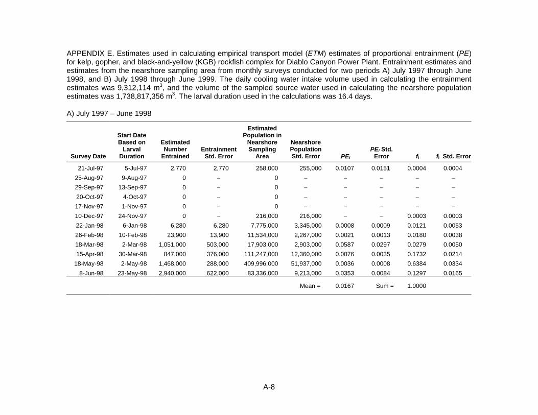
A-8
APPENDIX E. Estimates used in calculating empirical transport model (ETM) estimates of proportional entrainment (PE) for kelp, gopher, and black-and-yellow (KGB) rockfish complex for Diablo Canyon Power Plant. Entrainment estimates and estimates from the nearshore sampling area from monthly surveys conducted for two periods A) July 1997 through June 1998, and B) July 1998 through June 1999. The daily cooling water intake volume used in calculating the entrainment estimates was 9,312,114 m3, and the volume of the sampled source water used in calculating the nearshore population estimates was 1,738,817,356 m3. The larval duration used in the calculations was 16.4 days.
A) July 1997 – June 1998
Survey Date
Start Date Based on
Larval Duration
Estimated Number
Entrained Entrainment
Std. Error
Estimated Population in
Nearshore Sampling
Area
Nearshore Population Std. Error PEi
PEi Std. Error fi fi Std. Error
21-Jul-97 5-Jul-97 2,770 2,770 258,000 255,000 0.0107 0.0151 0.0004 0.0004 25-Aug-97 9-Aug-97 0 − 0 − − − − − 29-Sep-97 13-Sep-97 0 − 0 − − − − − 20-Oct-97 4-Oct-97 0 − 0 − − − − − 17-Nov-97 1-Nov-97 0 − 0 − − − − − 10-Dec-97 24-Nov-97 0 − 216,000 216,000 − − 0.0003 0.0003 22-Jan-98 6-Jan-98 6,280 6,280 7,775,000 3,345,000 0.0008 0.0009 0.0121 0.0053 26-Feb-98 10-Feb-98 23,900 13,900 11,534,000 2,267,000 0.0021 0.0013 0.0180 0.0038 18-Mar-98 2-Mar-98 1,051,000 503,000 17,903,000 2,903,000 0.0587 0.0297 0.0279 0.0050 15-Apr-98 30-Mar-98 847,000 376,000 111,247,000 12,360,000 0.0076 0.0035 0.1732 0.0214
18-May-98 2-May-98 1,468,000 288,000 409,996,000 51,937,000 0.0036 0.0008 0.6384 0.0334 8-Jun-98 23-May-98 2,940,000 622,000 83,336,000 9,213,000 0.0353 0.0084 0.1297 0.0165
Mean = 0.0167 Sum = 1.0000
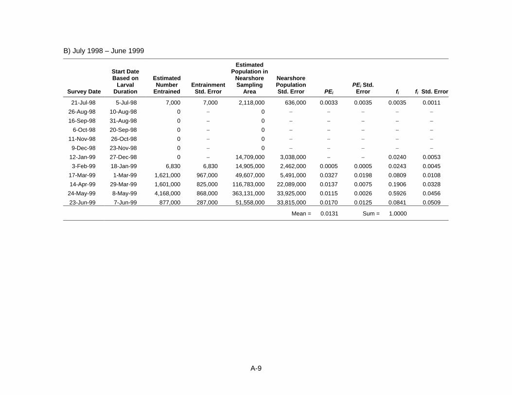
A-9
B) July 1998 – June 1999
Survey Date
Start Date Based on
Larval Duration
Estimated Number
Entrained Entrainment
Std. Error
Estimated Population in
Nearshore Sampling
Area
Nearshore Population Std. Error PEi
PEi Std. Error fi fi Std. Error
21-Jul-98 5-Jul-98 7,000 7,000 2,118,000 636,000 0.0033 0.0035 0.0035 0.0011 26-Aug-98 10-Aug-98 0 − 0 − − − − − 16-Sep-98 31-Aug-98 0 − 0 − − − − −
6-Oct-98 20-Sep-98 0 − 0 − − − − − 11-Nov-98 26-Oct-98 0 − 0 − − − − − 9-Dec-98 23-Nov-98 0 − 0 − − − − −
12-Jan-99 27-Dec-98 0 − 14,709,000 3,038,000 − − 0.0240 0.0053 3-Feb-99 18-Jan-99 6,830 6,830 14,905,000 2,462,000 0.0005 0.0005 0.0243 0.0045
17-Mar-99 1-Mar-99 1,621,000 967,000 49,607,000 5,491,000 0.0327 0.0198 0.0809 0.0108 14-Apr-99 29-Mar-99 1,601,000 825,000 116,783,000 22,089,000 0.0137 0.0075 0.1906 0.0328
24-May-99 8-May-99 4,168,000 868,000 363,131,000 33,925,000 0.0115 0.0026 0.5926 0.0456 23-Jun-99 7-Jun-99 877,000 287,000 51,558,000 33,815,000 0.0170 0.0125 0.0841 0.0509
Mean = 0.0131 Sum = 1.0000
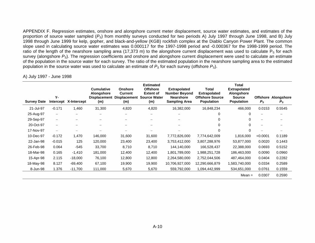
A-10
APPENDIX F. Regression estimates, onshore and alongshore current meter displacement, source water estimates, and estimates of the proportion of source water sampled (PS) from monthly surveys conducted for two periods A) July 1997 through June 1998, and B) July 1998 through June 1999 for kelp, gopher, and black-and-yellow (KGB) rockfish complex at the Diablo Canyon Power Plant. The common slope used in calculating source water estimates was 0.000117 for the 1997-1998 period and -0.000367 for the 1998-1999 period. The ratio of the length of the nearshore sampling area (17,373 m) to the alongshore current displacement was used to calculate PS for each survey (alongshore PS). The regression coefficients and onshore and alongshore current displacement were used to calculate an estimate of the population in the source water for each survey. The ratio of the estimated population in the nearshore sampling area to the estimated population in the source water was used to calculate an estimate of PS for each survey (offshore PS). A) July 1997 - June 1998
Survey Date Y-
Intercept X-Intercept
Cumulative Alongshore
Displacement (m)
Onshore Current
Displacement (m)
Estimated Offshore Extent of
Source Water (m)
Extrapolated Number Beyond
Nearshore Sampling Area
Total Extrapolated
Offshore Source Population
Total Extrapolated Alongshore
Source Population
Offshore PS
Alongshore PS
21-Jul-97 -0.171 1,460 31,300 4,820 4,820 16,382,000 16,848,234 466,000 0.0153 0.5545 25-Aug-97 − − − − − − 0 0 − − 29-Sep-97 − − − − − − 0 0 − − 20-Oct-97 − − − − − − 0 0 − − 17-Nov-97 − − − − − − 0 0 − − 10-Dec-97 -0.172 1,470 146,000 31,600 31,600 7,772,826,000 7,774,642,009 1,816,000 <0.0001 0.1189 22-Jan-98 -0.015 125 120,000 23,400 23,400 3,753,412,000 3,807,288,976 53,877,000 0.0020 0.1443 26-Feb-98 0.064 -545 33,700 8,710 8,710 144,140,000 166,528,437 22,388,000 0.0693 0.5152 18-Mar-98 0.165 -1,410 181,000 12,400 12,400 1,801,789,000 1,988,251,728 186,463,000 0.0090 0.0960 15-Apr-98 2.115 -18,000 76,100 12,800 12,800 2,264,580,000 2,752,044,506 487,464,000 0.0404 0.2282
18-May-98 8.127 -69,400 67,100 19,900 19,900 10,706,927,000 12,290,666,879 1,583,740,000 0.0334 0.2589 8-Jun-98 1.376 -11,700 111,000 5,670 5,670 559,792,000 1,094,442,999 534,651,000 0.0761 0.1559
Mean = 0.0307 0.2590
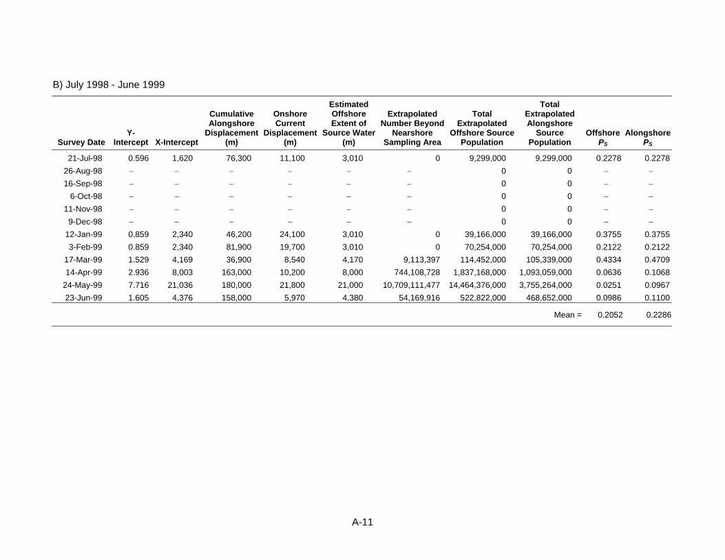
A-11
B) July 1998 - June 1999
Survey Date Y-
Intercept X-Intercept
Cumulative Alongshore
Displacement (m)
Onshore Current
Displacement (m)
Estimated Offshore Extent of
Source Water (m)
Extrapolated Number Beyond
Nearshore Sampling Area
Total Extrapolated
Offshore Source Population
Total Extrapolated Alongshore
Source Population
Offshore PS
Alongshore PS
21-Jul-98 0.596 1,620 76,300 11,100 3,010 0 9,299,000 9,299,000 0.2278 0.227826-Aug-98 − − − − − − 0 0 − − 16-Sep-98 − − − − − − 0 0 − −
6-Oct-98 − − − − − − 0 0 − − 11-Nov-98 − − − − − − 0 0 − − 9-Dec-98 − − − − − − 0 0 − −
12-Jan-99 0.859 2,340 46,200 24,100 3,010 0 39,166,000 39,166,000 0.3755 0.37553-Feb-99 0.859 2,340 81,900 19,700 3,010 0 70,254,000 70,254,000 0.2122 0.2122
17-Mar-99 1.529 4,169 36,900 8,540 4,170 9,113,397 114,452,000 105,339,000 0.4334 0.470914-Apr-99 2.936 8,003 163,000 10,200 8,000 744,108,728 1,837,168,000 1,093,059,000 0.0636 0.1068
24-May-99 7.716 21,036 180,000 21,800 21,000 10,709,111,477 14,464,376,000 3,755,264,000 0.0251 0.096723-Jun-99 1.605 4,376 158,000 5,970 4,380 54,169,916 522,822,000 468,652,000 0.0986 0.1100
Mean = 0.2052 0.2286