assessing the accuracy of the maximum likelihood estimator

Biometrika Trust

Assessing the Accuracy of the Maximum Likelihood Estimator: Observed Versus ExpectedFisher InformationAuthor(s): Bradley Efron and David V. HinkleySource: Biometrika, Vol. 65, No. 3 (Dec., 1978), pp. 457-482Published by: Biometrika TrustStable URL: http://www.jstor.org/stable/2335893 .Accessed: 27/04/2011 20:26

Your use of the JSTOR archive indicates your acceptance of JSTOR's Terms and Conditions of Use, available at .http://www.jstor.org/page/info/about/policies/terms.jsp. JSTOR's Terms and Conditions of Use provides, in part, that unlessyou have obtained prior permission, you may not download an entire issue of a journal or multiple copies of articles, and youmay use content in the JSTOR archive only for your personal, non-commercial use.

Please contact the publisher regarding any further use of this work. Publisher contact information may be obtained at .http://www.jstor.org/action/showPublisher?publisherCode=bio. .

Each copy of any part of a JSTOR transmission must contain the same copyright notice that appears on the screen or printedpage of such transmission.

JSTOR is a not-for-profit service that helps scholars, researchers, and students discover, use, and build upon a wide range ofcontent in a trusted digital archive. We use information technology and tools to increase productivity and facilitate new formsof scholarship. For more information about JSTOR, please contact [email protected].

Biometrika Trust is collaborating with JSTOR to digitize, preserve and extend access to Biometrika.

http://www.jstor.org

http://www.jstor.org/action/showPublisher?publisherCode=bio

http://www.jstor.org/stable/2335893?origin=JSTOR-pdf

http://www.jstor.org/page/info/about/policies/terms.jsp

http://www.jstor.org/action/showPublisher?publisherCode=bio

Biometrika (1978), 65, 3, pp. 457-87 457 With 11 text-figures Printed in Great Britain

Assessing the accuracy of the maximum lielihood estimator: Observed versus expected Fisher information

BY BRADLEY EFRON

Department of Statistics, Stanford University, California

AND DAVID V. HINKLEY

School of Statistics, University of Minnesota, Minneapolis

SUMMARY

This paper concerns normal approximations to the distribution of the maximum likelihood estimator in one-parameter families. The traditional variance approximation is 1/1.I, where 0 is the maximum likelihood estimator and fo is the expected total Fisher information. Many writers, including R. A. Fisher, have argued in favour of the variance estimate I/I(x), where I(x) is the observed information, i.e. minus the second derivative of the log likelihood function at # given data x. We give a frequentist justification for preferring I/I(x) to 1/.Io. The former is shown to approximate the conditional variance of # given an appropriate ancillary statistic which to a first approximation is I(x). The theory may be seen to flow naturally from Fisher's pioneering papers on likelihood estimation. A large number of examples are used to supplement a small amount of theory. Our evidence indicates preference for the likelihood ratio method of obtaining confidence limits.

Some key words: Ancillary; Asymptotics; Cauch-y distribution; Conditional inference; Confidence limits; Curved exponential family; Fisher information; Likelihood ratio; Location parameter; Statistical curvature.

1. INTRODUCTION

In 1934, Sir Ronald Fisher's work on likelihood reached its peak. He had earlier advocated the maximum likelihood estimator as a statistic with least large sample information loss, and had computed the approximate loss. Now, in 1934, Fisher showed that in certain special cases, namely the location and scale models, all of the information in the sample is recoverable by using an appropriately conditioned sampling distribution for the maximum likelihood estimator. This marks the beginning of exact conditional inference based on exact ancillary statistics, although the notion of ancillary statistics had appeared in Fisher's 1925 paper on statistical estimation.

Beyond the explicit details of exact conditional distributions for special cases, the 1934 paper contains on p. 300 the following intriguing claim about the general case WVhen these [log likelihood] functions are differentiable successive portions of the [information] loss may be recovered by using as ancillary statistics, in addition to the maximum likelihood estimate, the second and higher differential coefficients at the maximum.

To this may be coupled an earlier statement (Fisher, 1925, p. 724) The function of the ancillary statistic is analogous to providing a true, in place of an approximate, weight for the value of the estimate.

There are no direct calculations by Fisher to clarify the above remarks, other than calculations of information loss. But one may infer that approximate conditional inference based on the maximum likelihood estimate is claimed to be possible using observed properties

458 BRADLEY EFRON AND DAVID V. HINKLEY

of the likelihood function. To be specific, if we take for granted that inference is accomplished by attaching a standard error to the maximum likelihood estimate, then Fisher's remarks suggest that we use a conditional variance approximation based on the observed second derivative of the log likelihood function, as opposed to the usual unconditional variance approximation, the reciprocal of the Fisher information. Our main topics in this paper are (i) the appropriateness and easy calculation of such a conditional variance approximation and (ii) the ramifications of this for statistical inference in the single parameter case.

We begin with a simple illustrative example borrowed from Cox (1958). An experiment is conducted to measure a constant 0. Independent unbiased measurements y of 0 can be made with either of two instruments, both of which measure with normal error: instrument k produces independent errors with a N(O, a2) distribution (k = 0, 1), where u2 and U2 are known and unequal. When a measurement y is obtained, a record is also kept of the instrument used, so that after a series of n measurements the experimental results are of the form (a1, YO) ..., (a,n Yn), where a1 = k if y. is obtained using instrument k. The choice between instruments for the jth measurement is made at random by the toss of a fair coin,

pr(a, = 0) = pr(aj = 1) = i.

Throughout this paper, x will denote the entire set of experimental results available to the statistician, in this case (al, yl), ..., (an) Yn)

The log likelihood function 1,9(x), 1,9 for short, is the log of the density function, thought of as a function of 0. In this example

n1n 19(x) = const -log Oa,- (yj-)0)2/ao (121)

j=1 2j1aj

from which we obtain the maximum likelihood estimator as the weighted mean

a = ( YjIUaj) (Z 1/2 o)-1.

If we denote first and second derivatives of 1,9(x) with respect to 0 by 14(x) and 14(x), 4, and i, for short, then the total Fisher information for this experiment is

-f = var{4,(x)} = Et-1 (x)} = 1n(j/u02+ I/2).

Standard theory shows that &is asymptotically normally distributed with mean 0 and variance

var (&) 1/.f0. (1.2)

In this particular example X, does not depend on 0, so that the variance approximation (1.2) is known. If this were not so we would use one of the two approximations (Cox & Hinkley, 1974, p. 302)

1> IA lI/I(x), (1.3) where

I(x) =-4o = [ 2x] 0-X(x)

The quantity I(x) is aptly called the observed Fisher information by some writers, as distinguished from f0, the expected Fisher information. This last name is useful even though E(fo) * f0 in general. In the example above

I(x) = a/al + (n-a)/ o,

where a = z a>, the number of times instrument 1 was used.

Observed versus expected Fisher information 459

Approximation (1.2), one over the expected Fisher information, would presumably never be applied in practice, because after the experiment is carried out it is known that instrument 1 was used a times and that instrument 0 was used n - a times. With the ancillary statistic a fixed at its observed value, 0 is normally distributed wvith mean 0 and variance

var (Oa) = {a/a2 +(n-a)/ao}-1 (1.4)

not (1.2). But now notice that, whereas (1.2) involves an average property of the likelihood, the conditional variance (1.4) is a corresponding property of the observed likelihood: (1.4) is equal to the reciprocal of the observed Fisher information I(x).

It is clear here that the conditional variance var (O I a) is more meaningful than var (0) in assessing the precision of the calculated value 6 as an estimator of 0, and that the two variances may be quite different in extreme situations.

This example is misleadingly neat in that var(O la) exactly equals 1/I(x). Nevertheless, a version of this relationship applies, as an approximation, to general one parameter estimation problems. A central topic of this paper is the accuracy of the approximation

var (8J a) 1/I(x), (1.5)

where a is an ancillary or approximately ancillary statistic which affects the precision of 0 as an estimator of 0. To a first approximation, a will be equivalent to I(x) itself. It is exactly so in Cox's example. The approximation (1.5) was suggested, never too explicitly, by Fisher in his fundamental papers on ancillarity and estimation. In complicated situations, such as that considered by Cox (1958), it is a good deal easier to compute I(x) than 4. There are also philosophical advantages to (1.5). It is 'closer to the data' than 1/.If, and tends to agree more closely with Bayesian and fiducial analyses. In Cox's example of the two measuring instruments, for instance, an improper uniform prior for 0 on (-oo, oo) gives var (6 I x) = l1/I(x), in agreement with (1.5).

To demonstrate that (1.5) has validity in more realistic contexts, consider the estimation of the centre 6 of a standard Cauclhy translation family. For random samples of size n the Fisher information is X, = in. When n = 20, then 0 has approximate variance 0-1, in accordance with (1.2); the exact variance is about 0-115 according to Efron (1975, p. 1210). In a Monte Carlo experiment 14,048 Cauchy samples of size 20, with 6 = 0, were obtained, and Fig. 1 plots the resulting estimated conditional variances of 0 given I(x) versus 1/I(x). Samples were grouped according to interval values of /I(x). For example, 224 of the 14,048 samples had /I(x) in the range 0-170-0-180, averaging 0-175, and the 224 values of 02 had mean 0-201 and standard error 0-023. This gives the estimate

var{61 /I/(x) = 0.175} = 0-201 + 0-023

plotted in Fig. 1, since we know E{6I I(x)} = 0 by symmetry. Figure 1 strongly suggests the relationship

var {#I I(x)}) 1/I(x). (1.6)

This is a weakened version of (1.5). In translation families I(x) is ancillary, but it is only a function of the maximal ancillary a, the configuration statistic, i.e. the n - 1 spacings between the ordered values x(1) < ... <x(n). The stronger statement (1.5) is verified for translation families in ??2 and 8. We prefer (1.5) to (1.6) because var(Ola) is more relevant than var{6fI(x)} as a measure of precision for 0; in principle (Fisher, 1934) inference about 6 is conditional on a.


The implications of (1.5) are considerable. If I(x) = 15 in the Cauchy example, a not very remarkable event since pr {I(x) > 15}! 0.05, then the approximate 95% confidence interval for 0 is

0+ 1.96/415, (1.7) rather than

O+ 1.961110 (1.8)

as suggested by (1.2). The latter interval is too wide, having conditional coverage probability of 98% rather than the normal 95%. Given the equally unremarkable event I(x) = 6, interval (1.8) is too narrow, having conditional coverage probability of only 87%. These numerical comparisons presuppose accuracy of normal approximations, which is justified in ?4.

020 -

Est. var. +st. err.

* i / Theoretical 010 -i approx. (1.5)

005 / Upper 95%

Median point

,\~~~~~~~~~~~~~~~~~~~~~~~~~~4 0 005 0.10 0Z20 I-1

Fig. 1. Cauchy location 0. Monte Carlo estimates of conditional variance of maximum likelihood estimate 0 given the observed information I(x). Sample size n = 20; 14,048 samples.

The purpose of this paper is to justify (1.5) for a wide variety of one-parameter problems. The justification consists of detailed numerical results for several special examples involving moderate sample sizes, in addition to the general asymptotic theory. The results are presented in the following order: ? 2 gives an outline of the theory for translation families; ? 3 contains two detailed examples of this theory; ? 4 deals with confidence interval interpretations for the results of ? 2; ? 5 outlines the more complicated theory appropriate for nontranslation problems; ? 6 follows with an example; ?? 7 and 8 present details of the asymptotic theory; ? 9 contains brief concluding remarks, together with some further references and historical notes.


2. TRANSLATION FAMIIES

2* 1. Conditional variance approx$mation8 The theory of ancillarity and conditional inference for translation families was developed

by Fisher (1934). Here we will use Fisher's theory to justify (1.5), and its higher order corrections, in translation families. Section 4 contains the analogous results for approximate normal confidence limits based on (1.5). In ? 5 the general one-parameter problem is reduced to approximate translation form by a transformation argument. The treatment in this section is presented in outline form, more careful calculations being reserved for ? 8.

Suppose then that x1, ..., xn are independent and identically distributed with density f0(xl) = fo(x1 - 0). The data vector x can be reduced to the sufficient statistic (0, a), where #(x) is the maximum likelihood estimator and a(x) is the ancillary configuration statistic, representable as the spacings between successive order statistics, X(2) - (l)... X(n)-X (n-)

Because a is ancillary, its density g(a) does not depend on 0. The conditional density, with respect to Lebesgue measure, of 0 given a is of the translation form

fo(# Ia) = ha( - 0). (2.1)

The Jacobian of the transformation from the ordered xi values to (#, a) is a constant not depending on x, which implies that the density of x can be written

fg(x) = cg(a) ha(& -O) (2.2) for some constant c.

The likelihood function likx (0) is f0(x) thought of as a function of 0, with x fixed at its observed value. Fisher's (1934) main result relates f8( I a) = ha(#- 0) to likx(O): for any value of t = 8(x) -0,

ha(t) likx{&(x) - t} (2.3) ha(O) -likx{(x)}

This result, which is derived immediately from (2.2), looks simple but is in fact a powerful computational tool. Given the data vector x, it is computationally easy to plot the shape of the likelihood function likx(O). Reflection of this curve about its maximum point 8(x) then gives the conditional sampling density fg(#I a), which might otherwise be thought difficult to compute. The word 'shape' is necessary here since (2.3) determines ha(t) only relative to its maximum ha(O). Integration is necessary to determine the correct multiple, that which integrates to one. Fisher's tour de force was completed by noting that fully informative frequentist inferences about 0 should certainly be made conditional on the ancillary a, so that the likelihood theory leads easily and naturally to the appropriate frequentist theory.

To see how (2.3) applies to the phenomenon pictured in Fig. 1 suppose, for the moment, that lik_(O) happens to be perfectly normal shaped; that is,

lik (0) = exp [- IC2{ - #(X)}2] (2.4)

for some positive constant C2. Then (2.4) and (2.3) quickly give

fo(#I a) = hJ(- 0) = (2ff/c2)- exp { - iC - )2}.

In other words, a normal-shaped likelihood function implies that, conditional on a, # is

normally distributed with mean 0 and variance

var (81a) = l/6a. (2.5)


In the notation of ? 1, where l0(x) is the log likelihood function log likx(6), and dots indicate differentiation with respect to 0, (2.4) gives c2 =-4a = I(x), so that (2.5) is an exact form of (1.5),

var (#I a) = I /I(x). (2.6)

What if the likelihood function is not perfectly normal shaped ? As n gets large the likelihood will approach normality, assuming some mild regularity conditions on the form of f0(x), and we can use this fact to obtain asymptotic expansions for the conditional mean and variance of G given a. These expansions involve the higher derivatives of the log likelihood function, say forj = 3,4,

-(? [a' lo(x)] [ a' j0=0(x)l

all of which are zero in the normal case (2.4). We also use the notation l( 2) = 4 where convenient. Notice that (2.2) implies

- [ = a logha( ] 0= ( ) [a logha(t)

which says that the I(J) are functions of x only through a and are themselves ancillary statistics. This same statement applies to the observed Fisher information I(x) =-4.

LEMMA 1. In translation families satisfying the regularity conditions stated in ? 8,

var (#l a) = I-{1 + (J2/I3 -JK/1I2) + op(n-1)}, E(#j a) = 0- JJ/I2 + op(n-1), (2.7)

E{(G- )2 la} = I{1 + 32 1K) + op(n1)}, (2.8)

where I = I(x) =--[(x), J = l.3)(x), K - -l 4)(x). (2.9)

The proof of Lemma 1, which is an elaboration of the argument leading from a normal- shaped likelihood to (2 6), is given in ? 8, along with appropriate regularity conditions.

The terms in round brackets in (2.7)-(2.8) are of order OP(n-1) or smaller. In particular var (Ia) in (2.7) can be written

var (#I a) = I-1{1 + O?(n-1)}, (2.10)

which verifies (1.5). Lemma 2, in ?2-2, provides the final justification for (1.5) being an improvement over 1/4. The approximate normality of the likelihood function, which is used to prove Lemma 1, also ensures that the conditional distribution of # is approximately normal, given Fisher's result (2.3). Results directly related to conditional confidence intervals for 0 are described in ? 4.

In special cases the higher order terms in the left-hand side of (2.7) can be evaluated, giving expressions for var (O I a) more accurate than (1.5). This is demonstrated by the two examples of ? 3 and the brief discussion of the Cauchy translation problem in ? 8.

Even though the maximal ancillary a consists of I(x) plus the higher order derivatives I(i) (j = 3, 4, ...), the conditional variance var (#I a) is asymptotically equivalent, to within terms of order n-2, to a function of just I(x), namely /I(x). To put it another way, I(x) =-4 recaptures most of the information lost by considering only 8(x) instead of the full sample x. Some informal calculations to this effect were carried out by Fisher (1925). Roughly speaking, the pair (& 4) is the sufficient statistic for the two-parameter exponential family which best approximates the family f09(x) near the true value of 0; see ? 7 below.


2-2. Statistical curvature and comparison of variance approximations How different, numerically, is the conditional variance approximation I/I(x) from the

unconditional approximation 1/1.? An asymptotic answer can be given in terms of the statistical curvature ye,, as defined by Efron (1975, ?? 3, 5). Suppose that each xi has density function f0(x1), not necessarily of translation form, and define for j, k = 1, 2 the moments

IWgf(x)[ a2 logf { logf ) i k

~j(0) = EI a

Hf(l ox)+E 9(1

assuming these exist. Then the statistical curvature of f0(x1) is

Ye = (v02 v20-v 1)12/v 2. (2.11)

This curvature is a measure of the deviation of f0(x1) from exponential family form and is invariant under monotone reparameterization. One interpretation is that y2 f.f is the residual variation in to after linear regression on l,. For one-parameter exponential families ye = 0, and in such families I(x) = f, so that the two variance approximations being considered are equal. The statistical curvature of 19(x1, ..., x.) is ye/In.

The relationship between y9 and the variance approximations is given by the following result.

LEMMA 2. If x1, ..., x. are independent and identically distributed with density function fe(xl) satisfying the regularity conditions stated in ? 8, then as n -+ oo

Vn{I(x)/fo - 1}) ,N(0, y2). (2.12)

A proof is given in ? 8. Fisher (1925) indirectly suggests (2.12). In a translation family .10 = f and ye9 = y are constants, so that (2.12) can then be written

as I(x)/lf = 1 +O(n-i). Combined with (2 10), this easily leads to

var (#I a)-/II(x) O p(n-_), (2.13)

which shows that (1.5) is a valid and useful asymptotic approximation. Granting that var (# I a) is a more meaningful measure of variance than var (a), we see that I/I(x) is a better variance approximation than 1/f by a half order of magnitude, in the usual exaggerated sense of asymptotic comparisons. The numerical results for the Cauchy translation problem in ? 1 and the two examples in ? 3 show that the improvement can be substantial even for moderate sample sizes.

Suppose that we are interested in estimating a monotone function of 0, say a= =(8), rather than 0 itself. It is easy to verify that the observed Fisher information for a, say 1(0)(x), is related to that for 0 by

I(0f)(x) = I(x) (dO/d&)2. (2.14)

The expected Fisher information transforms in the same way. Since the maximum likelihood estimator maps the same way as does the parameter, & = a(8), the notation d#/d& is un- ambiguous, and equals [dO/da],f0. A standard expansion argument proceeding from Lemmas 1 and 2 shows that (1.5) is valid for a, in the sense of (2.13), that is

var (ala)-/IX )(x) - II(n ). (2.15)

17*


If we wish to compare confidence intervals for 0, conditional versus unconditional as at (1.7) and (1.8), the ratio of the lengths of conditional and unconditional intervals is

{1(x)1/A#}1. (2.16)

Lemma 2 implies that {I(x)/1f}* has, asymptotically, a normal distribution with mean 1 and standard deviation r,I(2In). For the Cauchy translation family y2 = 2 5, so that with n = 20 the standard deviation of {I(x)/1.,}ti is approximately 0- 18. We expect large variability in {I(x)/,f}i in this situation, which is indeed the case. Increasing n to 80 in the Cauchy problem reduces the standard deviation of {I(x)/J0}i to 0 09, so that conditioning effects become considerably less important.

3. EXAMPLES OF TRANSLATION FAMILIES

We illustrate the theory of the preceding section using two particularly simple examples of symmetric translation families due to Fisher.

Example 3'1: Fisher's normal circle. The first example is the circle model (Fisher, 1974, p. 138), where the data consist of a two-dimensional normally distributed vector x, covariance matrix the identity, whose mean vector is known to lie on a circle of known radius po centred at the origin. That is,

E(xT) = po(cos 0, sin 0). (3.1)

Having observed x, we wish to estimate the unknown 0. Note that given n independent observations xl, ..., x on this model the sufficient statistic x = E x,iIn satisfies (3.1) with

poln in place of po. If the data vector x has polar coordinates (0, rpo) then 0 is the maximum likelihood estimate

of 0, and r = II x II /pO is ancillary. The density is of the form (2 2), with a replaced by r, so that we can apply the theory of ? 2, even though (3.1) does not look like a standard translation problem. The density g(r) is noncentral chi, while the conditional density

fog(# I r) = h,(- 0) is the 'circular normal',

c-1 exp {p2r cos ( -6)} (3.2)

Here we are assuming that # given 0 ranges from 0-fi to 0 + i, for the sake of symmetric definition. The constant c equals 27rIO(p2r), in the standard Bessel function notation.

Now we can apply Lemma 1 of ? 2. From (3.2) we calculate

1(.i) = -)ijpo2r (j=2,4,).. (3 )

and IW) = 0 for j odd. The Fisher information A6, is constant,

>a= f=po2 (3.4)

Using I(x) =-t = rf, 1(X3) = 0, 1(4) = rf, from (3.3) and (3.4), (2.7) can be written

var( Ir)-{{1 + 1/(2rf)}. (3.5)

The exact conditional variance of # given the ancillary statistic r is calculated from (3.2) to be

var (8Ir) ={ t2exp (rf cost)d)t exp (rfcost) dt). (3.6)

Observed versus expected Fisher information

Figure 2 compares (3.6) with (3.5). For values of p2 = f > 8 it can be shown that at least

95% of the realizations of rJ = I(x) will be greater than 4. We see that approximation (1.5), var(Olr)=l/(rf), is quite acceptable in the range 1/(rf) 0.25, and that the improved approximation (3.5) derived from Lemma 1 is very accurate.

The exact variance (3.6) can be expressed in terms of Bessel functions, whose expansions lead to (3-5).

Example 3-2: Fisher's gamma hyperbola. Fisher's hyperbola model, introduced in connexion with his famous 'problem of the Nile' (Fisher, 1974, p. 169), involves two independent scaled gamma variables whose means are restricted to lie on an hyperbola. Thus we observe x = (xl,x2) such that xi = e0Gm1 and x2 = e-00m2' where Gi indicates a variable with

density xm-le-z/r(m) on (0,oo). The Fisher information for 0 is f = 2m. The maximum likelihood estimate of 0 is 8 = log (x1/x2). This is illustrated in Fig. 3.

0.1 I-1 = (rJ)-1

Fig. 2 (left). Exact conditional variances, circles, of 0 given r compared with approximations (2.7), curves, for the circle and hyperbola models. Dotted line, approximation (1.5).

The ancillary statistic in the hyperbola which are hyperbolae 'parallel' to the curve It has density

Fig. 3 (right). Fisher's gamma hyperbola model. x = (l, x2), a pair of independent gamma variables with index m, whose means lie on solid curve. Broken curve, one orbit hyperbola

for ancillary statistic r.

model is r = 1(x1 2)/m, the level curves of of possible mean vectors, as shown in Fig. 3.

2T2m 2m- g(r) = r(m)}r2m- exp {- 2mr cosh (t)} dt,

the conditional density of 8 given r being

f(8 I r) = exp{ - 2mr cosh (8 - 6)}/ exp { - 2mr cosh (t)} dt. (3-7)

In other words, this is another nonobvious example of form (2.2).

465


The log likelihood derivatives, from (3.7), are

iV) = --2mr =-rf (j = 2,4, ...), (38)

1W) = 0 for j odd, so that I(x) = rf as in the circle model, and (2.7) gives

var( Ir)-7{1- /(2rf)}. (3.9)

This differs only in the sign of the second term from the corresponding formula (3.5) for the circle model. The actual conditional variance var(gI r), obtained by integrating (3.7), can also be expressed as a function of rf. The comparison of (3.9) with the actual conditional variance, Fig. 2, is almost exactly the same as for the circle model, except that here the deviations from the line var(glr) = I/I(x) = 1/(rf) go in the opposite direction.

4. CONDITIONAL CONFIDENCE INTERVALS FOR THE LOCATION PARAMETER

Our results so far have been presented mainly in terms of variances, it being understood that these are of most interest in conjunction with a normal approximation for 0-0. The expansion theory of ? 2 can be expressed directly in terms of conditional confidence intervals, an idea we now pursue explicitly.

As before, consider first the situation where lik_(G) happens to be perfectly normal shaped, so that (2.4) holds with c2 = I(x). There are two consequences of this relating to standard confidence interval methods. First, 0 has an exact normal distribution conditional on a, so that

U(X) = J(x) (8_ 0)2 (4.1)

is exactly a X2 variable conditional on a. If the upper p poillt Of X2 is denoted x2(p), then level p conditional limits on 0 are + ? {X2(p)/I(x)}*. The other standard method of setting confidence limits is based on

v(x) = 2{tl(x)(x) - 10(x)}, (4.2)

which also has an exact Xl distribution conditional on a. Although in general the likelihood function is not exactly normal shaped, it is approxi-

mately so for large n, and the same expansion methods used to confirm (1.5) also show that u(x) and v(x) defined above are asymptotically X2 conditional on a. More formally, we have the following result, proved in ? 8.

LEMMA 3. For translation families satisfying the regularity conditions in ? 8, the statistics u(x) and v(x) defined by (4.1) and (4.2) satisfy

pr {u(x) > u0jI a} = (1 -di-d2) pr (X12 > uO) + d pr (X2>u) + d2pr( uO) + o,(n-1), (4.3)

pr (v(x) > uo I a} = (1 - d1-d2) pr (X1 , uO) + (d2 + dl) pr (X23 > uo) + or(n1), (4.4)

where di =-K/(8I2) and d2 = (5j2)/(2413), with I, J and K as defined in (2.9). Because d, and d2 are both O(n-1), (4.3) and (4.4) imply

I(x)(_ 0)2Ja = X2+ O(n1), 2(1-10)ja = X2+OP(n-1). (4.5)

Note that the latter result is a conditional version of Wilks's famous theorem, and establishes that a standard method has the correct conditional properties.


The results (4.5) are superior to the unconditional result

.>f#( 0)2 = X2 + 0p(n-1) (4.6)

in a sense similar to (2. 13). As we pointed out in ? 2 2, the degree of superiority is determined by the curvature.

To investigate the practical validity of (4.5), we return to the Cauchy translation problem discussed in ? 1. We have generated 20,000 samples of size n = 20 and computed the empirical frequencies with which fo(6- 0)2, I(x) (0- 0)2 and 2(1 - 1) exceeded X2(P) for p = 0 05 and 0.01, broken down by interval values of I(x). Figure 4 graphs the results which show convincing evidence in support of (4.5) and dramatic conditional effects on the unconditional statistic (4.6). Note that the likelihood ratio method agrees better numerically with the chi-squared approximation than does the method based on 0. The expansions (4.3) and (4.4) indicate that this may be true in general, since pr (X2 > uO) is an increasing function of q.

0.15 _ o *5. ..15*. Est. prob.

+ st. err.

0.10-~~~~~~~~~~~~~0 0*10_*.*

,0

0

0 .0

001 _0

0.~ ~ ~ ~~ ~~~~~~~~~~~~~~~~~~~1

& 2 5 10 15

Fig. 4. Monte Carlo estimates of pr (statistic > c I I) with c = 3-84, shown by closed circles, and c = 5.99, open circles, for three likelihood statistics in the Cauchy location model, n = 20. Statistics: 2(l -1l) shown by solid curve; 1( 0-0)2, dashed curve; jf(O - 0)2, dotted curve.

Estimates from 20,000 samples.

5. NONTRANSLATION FAMLIES

This section discusses an example of a nontranslation problem in which a version of (1.5) can be seen to hold. We will use this example to introduce definitions appropriate for general nontranslation problems. The example is totally artificial, being in fact a simple variant of


Fisher's circle model, but furnishes a useful starting point because of its simplicity. A nontranslation problem of a more realistic nature is discussed in ? 6, again showing (1.5) at work.

We have not been able to provide a theoretical justification for these results in general, and pathological counterexamples are easy to construct, but nevertheless the examples suggest that (1.5), suitably interpreted, has wide validity.

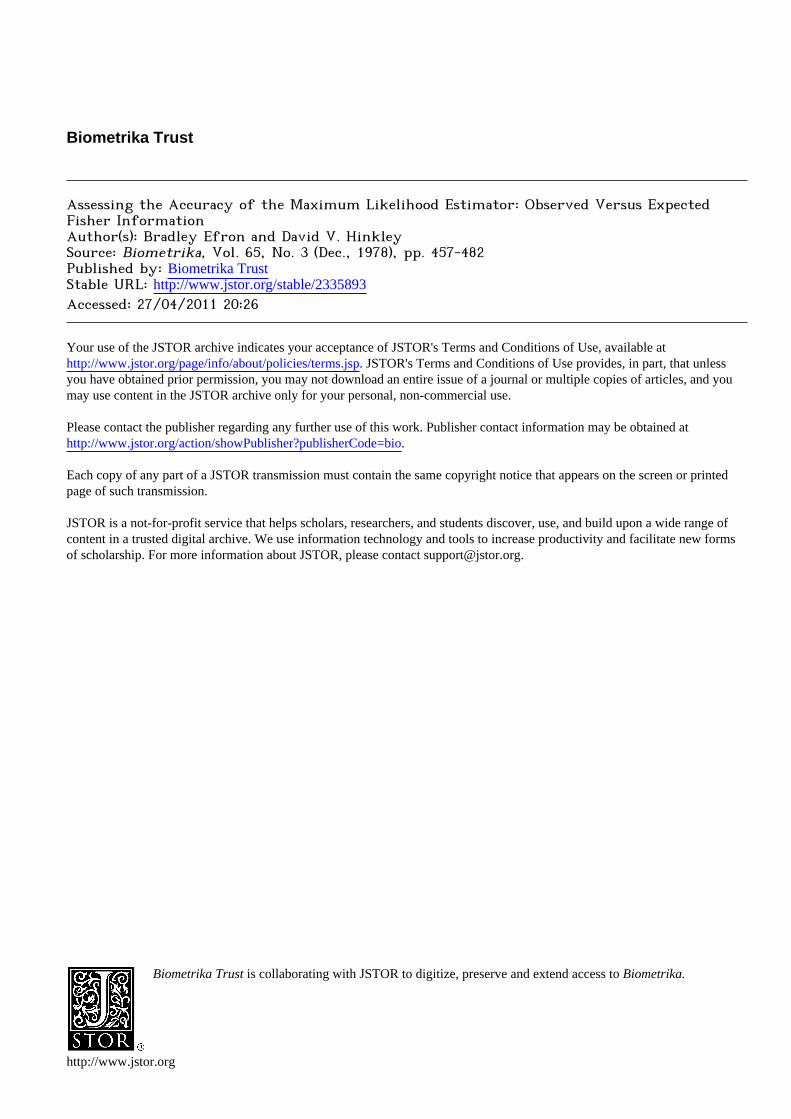
Figure 5 illustrates a model in which the data vector is bivariate normal, covariance matrix the identity, and with mean vector constrained to lie on a spiral, instead of Fisher's circle; that is

E(x) = =[cos 6 - po,sing] P=Po , <Po 5 sin( ) +p0cosQj' PaoP X Po. (6.)

The spiral is generated by the enid of a thread unwinding from a circular spool of unit radius. By definition the thread has length po at 0 = 0, which implies that it has length po = po-6 at 6. At 6 = +pO, we have po = 0, which accounts for the restriction in (5.1). We wish to assign some measure of accuracy to the maximum likelihood estimate 6 on the basis of the observed x. The sample size here is n = 1, but under repeated sampling essentially the same model holds with x replaced by x = E xi/n.

spoo~~

Q(x) = q

Anl;gle /i

Fig. 5. Spiral model. x = (X1 X2), bivariate normal with identity covariance matrix and mean go on a logarithmic spiral shown by solid curve. Maximum likelihood estimate 0 is angular coordinate of straight thread on which x lies. Ancillary statistic has constant value q on parallel spiral

through x, dashed curve.

It is easy to calculate that the Fisher information and curvature for the spiral model are 9 = p3 and yV = l/pa, and that having observed x, the maximum likelihood estimate 8(x)

is the angular coordinate of the thread upon which x lies. The vector fl is the closest point to x on the spiral of possible mean vectors. When pa is large the curvature is small, and we exQpect small conditioning effects, the reverse being true when p09 is small.


The geometry of Fig. 5 and familiarity with the bivariate normal distribution suggest that Q(x), the signed distance of x from Pou, should be approximately ancillary, with a limiting N(O, 1) distribution as P6o gets large. We take the sign of Q(x) positive if x is closer to the spool than , and negative if it is farther from the spool. Figure 5 shows that the level curve Q(x) = q is a parallel spiral having thread everywhere q units shorter than that for the mean vector.

We intend to use Q(x) as an approximate ancillary, conditioning upon the observed value of Q as we did upon a in the translation case. Both D. A. Pierce and D. R. Cox suggest this use of Q in the discussion following Efron (1975). Table 1 displays the marginal density of Q(x) for four values of 6 and eight values of Q = q. The four 6 values are chosen such that Po = Po-6 = 18, 416, 432, 464; it is irrelevant which combinations of po and 6 are used to get these values of po9. The density would be constant across rows if Q(x) were a genuine ancillary. We see that it is nearly constant, tending toward the N(O, 1) density as pc9 -* o.

The marginal densities in Table 1 were obtained by numerical integration of the bivariate normal density along the spiral Q(x) = q. To avoid certain problems of definition, for each p6, the integration was restricted to points on this spiral with angular coordinate in the interval 6 + Ir. Notice that if p9 - q < Ir, then the spiral runs into the central spool before the lower limit 6- Ir is reached. This end effect seriously distorts a few of the more extreme calculations, as indicated in the tables.

Table 1. Exact marginal density of asymptotic ancillary statistic Q(x) at q for Po = 48, 416, 432, 464

N(O, 1) Q = q po= 48 po = 416 pe = 432 pe = 464 density -2 0 07 0.07 0-06 0.06 0.05 -1.5 0d16 0.15 0Q15 0-14 0-13 - 1 0.29 0.27 0.26 0.26 0.24 -0*5 0.39 0.38 0.37 0.36 0.35

0 0-41 0.40 0.40 0.40 0Q40 1 0.19 0.21 0-22 0.23 0.24 1.5 0.08* 0 10 0.11 0.12 0.13 2 0.02* 0.04 0.04 0.05 0.05

Last column gives the N(O, 1) density, corresponding to the limiting case P -+ oo. *: substantial distortion by end effects.

The observed Fisher information I(x) is

I(x) = {1 -y0Q(x)}.f4 = p0(p0-q), (5.2)

where O = 8(x) and q = Q(x). We will also use the notation I(q, I) = 1(c) to emphasize the partition of x into the approximate ancillary Q(x) = q and the estimate 0. Rather than directly verifying that var (#I q) 1 /I(q, 0), which is in fact true, we will first make a 'variance stabilizing' transformation of parameter, to put the problem in an approximate translation form, where we can expect our approximation theory to work better. Fraser (1964) makes a similar effort using a different technique.

For a fixed value of q consider the transformation 06 * Oq defined by

d -q = 4II(q,) = 4{pc(pc-q)}. (5.3)

Equation (2.14) shows that I(^e)($) = I(x)f{p8(p - q)} (5.4)


for Q(x) = q. In terms of the new parameter X2, the observed Fisher information is one for every x on the level curve Q(x) = q. Since we intend to make conditional statements given Q(x) = q, it causes no trouble to use a different transformation for each value of q. Relation (1.5) then becomes simply var ($q I q) 1. Notice that if this is true, then transforming back to 0 gives

var (# I q) , var (Oa I q) Ad)~(- = I~ () '(5'5)

which is (1P5). There is one more level of approximation in (5.5) than in var($, Iq) 1 which, to reiterate, is one reason for making the transformation (5 3).

Table 2 shows that the quantity q -aq does indeed have nearly the right mean and variance, 0 and 1 respectively, for the cases considered. The worst case is q = 0, p6 = 18, for which the variance is 1-10. The case q = 2 with po = 18 looks terrible, but that is due to the end effect previously mentioned.

Table 2. Mean and variance of $q- q for p6 = 18, 116, 132, 164.

q pe = 18 pe = 416 pe = 132 peo = 64 - 2 -0*02 1*04 - 0.01 1.02 -0.00 101 -0.00 101 -1 -002 1.06 -001 1*03 -000 1.01 -0.00 1*01

0 -002 1.10 -0.01 1'04 -0.00 1.02 -0.00 1*01 1 0Q05* 0Q99* -0.01 1.05 -000 1.02 -0.00 1*01 2 0Q49* 0.58* -0.00 1*06 - 0*00 1*03 -000 1.01

*: substantial distortion by end effects.

Other moments of $q-aq were calculated, all of which indicated good agreement with a standard normal distribution. For example, E(I A-OIa) was within 4%, the worst case again being q = 0, Po = 18. Another advantage of variance stabilizing transformations is that they tend to improve normality. In our two examples, q-bq was more nearly normal than 0-6. This suggests forming conditional confidence intervals for 6 by computing $q ? Zjp, where zi, is the upper 1p point for N(0, 1), and transforming back to the 6 scale. This method agrees with # + zip/tI(x)}i to first order, but can give quite different results for small sample sizes.

To summarize the results for the spiral model, Q(x) contains very little direct information about 0, but its observed value considerably influences the variance of #. For example, (5.2) shows that if pe = 116, then I(q, 0) varies from 24 to 8 as q varies from -2 to 2, causing a threefold change in the variance approximation I/I(x) for #. In other words, Q(x) acts as an effective ancillary statistic.

We now extend the definitions of Q(x) and bq to an arbitrary one parameter family, say F = {fg(x), 6 E ?}, ED an interval of R1, satisfying the regularity conditions of ? 8.

Define

Q(x) 1-I(x)/J (5.6)

which agrees with (5 2). Lemma 2 shows that VnQ(x)-N(O, 1) as n-coo, assuming that y6e is a continuous function of 0, that is Q(x) is asymptotically ancillary. We have already mentioned that (#, 4) acts like the sufficient statistic for the two parameter exponential family which best approximates F near any given point 6 in E). The statistic Q(x) is the function of (8, T4) linear in 4, for 8 fixed, which is asymptotically ancillary. The definition


of Q(x) is also motivated by the obvious geometrical considerations of Fig. 5, generalized in ?7.

From (5 6) we can write I(x) = I(q, 0) = (1 -yaq).f as before, since I(x) is a function of 0 and the observed value q = Q(x).

The general definition we will use for bq is

d n)

where n is the sample size of a random sample xl, ..., xn from some member of S. In making this definition, q is considered fixed and 0 variable. The mapping 0>bq is monotonic over intervals of 0 where I(q, 0) does not change sign. The possible difficulties of definition at points where I(q, 0) = 0 do not cause trouble in our examples. A discussion of the special nature of such points is given in ? 5 of Efron (1978).

In a translation family definition (5.7) automatically produces a linear function of the translation parameter, 0bq = Cq + dq 0, if the original 0 is any smooth monotonic function of the translation parameter.

By (2.14) and (5 7), the observed Fisher information for 0f, is

ID0)(x) = nI(x)/I(q, ) (5.8)

and is n for Q(x) = q. That is, I(00)(x) is constant on the level surface Q(x) = q. The choice of the constant equal to n keeps Oq and 0 the same order of magnitude. In the example of ? 6, as in the spiral example, we verify that Q(x) is close to ancillary, and that var ($q I q) 1/n in accordance with (1.5).

The transformation 0>bq defined by (5.7) is mainly of theoretical and conceptual convenience. Practical evidence certainly suggests that the likelihood is often more normal on the bq scale. But the derivation of Oq is often difficult and usually requires approximation; see ? 6. Moreover, if, as we believe, the results of ? 4 generalize, then

2(1- 10)Iq = 2(li, Q-I0) I q = X1+ Op(n-1), (5.9)

so that confidence limits for 0 can be derived directly from l(x). We emphasize that (5 9) has not been proved for the general case. Confidence limits for 0 can also be determined by taking the quadratic approximation in (0-0) to

ni($q0q)=| 4) = I(q,t)Idt.

The numerical results of ? 6 suggest that the direct likelihood method based on (5.9) is preferable.

A corresponding treatment of locally most powerful tests of Ho: 0 = 00 indicates that the appropriate standardized form of the score statistic is l00,/{I(x)}*, which is approximately N(O, 1) conditional on Q = q. In this form the score statistic is no more convenient than its asymptotic equivalents, since 0 must be computed; for an example, see Hinkley (1977).

What happens when we have r independent sets of samples from the same model? How would we compare the estimates? How would we pool the estimates? Answers to these questions are essentially given by Fisher (1925). Suppose that we have only (#, jj) for j = 1, ..., r. Then the appropriate pooled statistic is (#, I*), say, where # = E I Ojl I, and I= E Ij; G is second-order efficient according to Fisher's informal argument. The effective part of (Q1, ,Q) to first order, is presumably Q = (1 +Iff)y>1, where f. is the grand


total Fisher information. A reasonable conjecture is that (, ,Q.) is equivalent, to second order, to the statistics (#,Q) computed from the pooled likelihood function. Comparisons of the # would be made conditional on (Q1, ...,Q,), and would be asymptotically equivalent to normal-theory comparisons with sample weights I,. For example, in testing the equality of parameter values, the likelihood ratio statistic is

r r rA

W = 2 E('- 1j6) (l ,&-l2).' (Ij.0, - Oj-)2 J-1 1=1 j-1

under the hypothesis of equality. But the right-hand side is

, IJ(# _ 0)2 _ I 0)2,

which by extension of earlier arguments is approximately XT2_ conditional on

(Ql, .. ~Qr) =(ql .. qr)-

6. EXAMPLE OF A NONTRANSLATION FAMILY

We illustrate the theory of ? 5 for a simple nontranslation example, using Monte Carlo methods to estimate the conditional properties of the maximum likelihood estimate.

Let Xi = (X1, X20) for i = 1, ..., n be independent bivariate normal pairs with zero mean, unit variances and correlation 0. The two-dimensional sufficient statistic is

n n 81 = aX1iX2i, S2 = 2(X.2X+X2i))

i=l X=1

and the first derivative of the log likelihood function is

n0(-_ 02) 0S2 + (1 + 02) S1

to- (1 _02)2

Calculations for the Fisher information and curvature (2.11) are straightforward, yielding

a = n(l+ 02)/(1 _ 02)2 y2 - 4(1 _02)2/(1 + 02)3.

Some numerical values of both fo and y2 are given in Table 3. A qualitative interpretation of the curvature values is that our two-dimensional exponential family model is highly nonlinear for small 101, but nearly linear as 0 -- + 1. The effect of replacing fo by I(x) is potentially large for small I01

Table 3. Information, curvature, and parameter q0 for special bivariate model

l0 0 0.1 0.2 0-4 0-6 0.8 0.9 0-95 1

.4/n 1 1.03 1 13 1 64 3 32 12-65 50 14 200 OO

Ys 4400 3 81 3 28 1 81 0.65 0.12 0.024 0.0055 0

c0 0 0.100 0 204 0-435 0737 1.235 1 727 2 217 OO

The variance stabilizing transformation 0+Xq defined by (5.7) is equivalent to

kq = n-i Jf (1 -qyt)i dt.

As in many examples it is difficult to evaluate this transformation exactlv, but a good approximation can be obtained by substituting (1 -qyt)1-il 1- iqyg; recall that q is O(n.).


In the present case this substitution leads simply to

qo 00-q tan-1 0, (6.2) where

00= 2*tanh-1(602*)-tanh-1(60), { = 0(1 +02)-i.

The normalizing effect of the transformation 0 -+ 0fq is illustrated by plots of likelihoods and their normal approximations in Fig. 6 for a small data set with n = 20, s, = 12, 82 = 35. In each case the likelihood is graphed relative to its maximum. The observed informations, respectively I(x) and n, are used as variance inverses in the normal approximations, which are centred on the maximum likelihood estimates.

100 1.0 1

10 0 0

v-5 ~ ~ ~ ~ .0.5

4a 0 l0L

0.5 1.0 1.0 2*0

Fig. 6. Relative likelihood functions shown by solid curves, and normal approximations, dotted curves, for correlation 0 and transformed parameter a for bivariate normal sample with known N(0, 1) marginal distributions. Data: n = 20, s, = 12, 82 = 35, 0 = 0-7185, I(x) = 122-77,

q = 0O101, $b = 0 928.

Our interest is in whether Q(x) defined by (5.2) is approximately ancillary, and whether var ($q q) 1/n is accurate. Notice that 00 is the transformation which makes fo = n, so that the superiority of I(x) over 0 as a measure of precision conditional on Q(x) = q may be judged by comparing the conditional variances of q and $0. The preceding theory would indicate that conditional on q

var ($qq)-I/n = O(n-.),

but we have not proved this. The likelihood equation to = 0 has three solutions, two of which may be complex; the

frequency of multiple real zeros increases with curvature and with q. We computed 0 as a solution to the likelihood equation by iterating from an efficient estimate of 0, not the sample correlation. We simulated samples for n between 15 and 40, with 0 ranging between 0 and 0 9. The numbers of samples were 10,000, 50,000 and 10,000 for n = 15, 25 and 40 respectively. In each case results were recorded for twenty interval values of q in the 99% range -2 < q < + 2, there being approximately the same number of samples for each q interval.

From the simulation results it was quickly apparent that the range of values of 0 for which the approximate theory of ? 5 is accurate depends markediy on sample size. For that


1.01 (a) ? 1.0- (b) 0000 10 (c)

6~~~~~~~~0, 06 06009 060

0 00 *

05 10 0 0 0

-C p o 0 1 0 0 0

5 0 _o 0_ 0 0 0~ 0 * * 0

0 * 0 ~~~~~~~0

0

11n' pr t. of r

N(0 1)Orl1

I _ _ _ _ _I_ _ _ 0I 0*51005 1.0 0.5 1.0

Cum.-prob2 of N(O, 1) Cum. prob. of N(0, 1) Cum. prob. of N(2, 1)

Fig. 7. Empirical cumulative probabilities of approximate ancillary Q in correlation model against N(0, 1) cumulative probabilities. (a) n = 15, 0 = 0, 0.3; (b) n = 25, 0 = 0, 0-3, 0-5, shown by closed circles, and 0 = 0-6, open circles; (c) n = 40, 0 = 0-7, closed circles, and 0 = 0-9, open

circles. Numbers of samples exceed 10,000.

(a) n = 15, 0 = 0 (b) n =25, = 0 0

0 0 0

0 ~ ~ ~ ~ ~ ~ ~~ 0

St. var. 00

+st. err. 0 .*:~~ 0 0@0 0

o~~~~~~~~~~- o

* 00 _ 14 ~~~~~~~~~0000 o01 0 000 -

_ > *..0-3 0

0 0

0 0

l I I _ _ _ _ _ _ _ _ _ _ _

-2 0 2 -2 0 2

q 4n q n

(c) n 25,0 0-3 Q (d) n =40,0 0-7 0

0-3- 0 0

~~~1~~~~~ ~0 0-6- 00 0 00

0 **0* 0 0

o 0 ~ ~ ~~~~~~~~0 0

0 * ~~~~~~~~~~~~~~~0 0

0-3 0~~0 0 0~~~~~~~~~~~~~

0-2~

-2 0 2 -2 02

q In q 4n

Fig. 8. Monte Carlo estimnates of conditional variances of $,shown by closed circles, and of

4open circles, given Q = q in correlation model. Dashed line, theoretical approximnation, 1/n.


08

00

*~~~~ Vn

00.5.

-~ ~~ l%l

-2 0 2

q 4 qn

Fig. 9. Monte Carlo estimates of conditional mean of $s circles, given Q = q, and theoretical approximation, dahed line, in the correlation model with n = 25, 0 = 053, Estimates from

50,000 samples.

n ~~~~~~~~Est. prob. n ~~~~~~~~~+ st. err.:

o \..

=~~~~~~~~~~~~~~~~ \

-1 01

Fig. 10. Monte Carlo estimates of pr (statistic k 3*84 I Q = q) for three likelihood statistics in correlation model with n = 25, 0 = 0 3. Statistics: 2(l9-l@), shown by solid curve; n($a- q)2,

dashed curve; n(#o-,o)2, dotted curve. Estimates from 50,000 samples.


reason we give a comprehensive set of illustrations here. First, Fig. 7 contains normal plots of the empirical distributions of Q(x), a separate graph for each sample size. Several 6 cases are indistinguishable, but clearly as I 01 1 the approximate ancillarity of Q(x) breaks down.

Figure 8 contains plots of empirical conditional variances of both q and $0 for six repre- sentative cases. Standard errors for the estimated variances are indicated. These graphs confirm the theory to a remarkable degree. Particularly striking are the deviations from n-1 of the conditional variances of A0.

The approximation (6 2) is remarkably accurate for the conditional mean of q, which implies that the conditional mean of $0 deviates from 00. Figure 9 illustrates a typical case.

The final numerical results are concerned with approximate methods for obtaining confidence limits for 0. According to our theory, both n($q - #q)2 and 2(1- lo) are approximate

Xi variables conditional on q. In contrast n(0 - o)2, which is an approximate x2 variable unconditionally, does not have this property conditionally. Figure 10 contains empirical conditional tail probabilities for all three of these statistics corresponding to the value 3X84, nominal 0 05 probability, for the case n = 25, 0 = 0 3. Our speculative theory is nicely confirmed by these and similar results. As in the Cauchy case, ? 4, the likelihood ratio method gives the best agreement with the chi-squared approximation.

Note that even for n = 40 conditioning on q is likely to have an appreciable effect, because the coefficient of variation of I(x) is as hwigh as 0 3, its value at 0 = 0. Thus at n = 40 the unconditional variance approximation 1/. can easily depart by a factor of two from the conditional variance approximation.

7. CURVED EXPONENTIAL FAMILIES

The definition of the asymptotic ancillary statistic Q(x) at (5.6) is motivated by the geometry of curved exponential families. This section gives a brief description of the geometry involved. More details are given by Efron (1975, 1978).

We begin with a k-dimensional exponential family C, with density functions of the form

g9(x) = exp{JT X-+0(a)} (C E A, x E ), (7.1)

b(a) being a normalizing constant. The natural parameter space A and the sample space 8 are both subsets of Rk, A being convex. Corresponding to each a is the mean vector and covariance matrix of x,

B = E,(x), Qa = cova(x). (7.2)

The mapping from a to f is one to one, so C can just as well be indexed by f as by a. The space B = {fl(ca): a cA} is not necessarily convex.

A curved exponential family F is a one parameter subset of C, with typical density function say

f0(x) = exp (aTx x- 0), b09 = b(cy.g). (7.3)

Here 0 is a real parameter contained in 0, an interval of RB, and the mapping 0+ao, is assumed to be continuously twice differentiable; F is fully described by the curve Ji = {aq: Ge 0} through A, or equivalently by the curve B = {Fe = f(a): 6 0E} through B. All of our examples, except for those in ? 1, involve curved exponential families.

If C is two-dimensional, as in Figs 3 and 5, then for a given 6, the set Q(x) = q is a single vector. It is shown in ? 5 of Efron (1975) that this vector v has squared Mahalanobis distance q2 from F. in the inner product Q-1l: (v - flo)T -1(v -V go) - q2 This generalizes the geometric description of Q(x) given in Fig. 5, where Q,4 is the identity. A similar interpretation holds


for higher dimensional families C. The Cauchy translation problem may be thought of as a limiting case of a curved exponential family, as remarked at the end of ? 5 of Efron (1975).

We use the notation Q,i = D.,, and also 9 = dox0/dO, at = d2at/dO2. Suppose x1, ... xn is a random sample from some member f9 of .S. The average vector

x = Ex /n is a sufficient statistic for 0, and it is easy to verify that the derivatives of the log likelihood function are

4(x) = n3J (x-l,06), 4(i) = n&, (x-,lE)-'4- (7.4)

where fo = n&T Q6 &,6 is the Fisher information. Figure 11 illustrates two useful facts about solutions to the maximum likelihood equation

1(fl = 0, both of which follow from (7.4). (i) Given #, the set of x vectors for which 1t(i) = 0, that is for which # is a solution to the

likelihood equations, is the k - 1-dimensional hyperplane through PeJ orthogonal to 6&o, say

= { 6: &T(i-.,) = 0}. (7.5)

(ii) From (5.6) and (7.4),

Q(x) = n&T (x-fl)/(yafa). (7.6)

Therefore for a given #, the set of x vectors for which Q(x) = q is the k - 2-dimensional hyperplane contained in .o and orthogonal to 80, the projection of &x into Y.

0c at/

X S z XX ~~~~~Rc \ <??~~~plane

/~~~~~~~ Q(x) =q

Fig. 11. Geometry of maximum likelihood estimation in a three-dimensional curved exponential family. Curve .B, values of go = E8(f); plane 2t orthogonal to At, vectors x for which 0 t; vector

St, projection of &t in 2t, is q axis when 0 = t.

So far we have discussed two 'coordinates' of x of particular interest, namely # and q. The remaining k -2 coordinates necessary to specify i completely are higher order ancillaries, corresponding to the lS.J) for the translation problem. We can replace x by the sufficient statistic (#, a), where a represents the k-I coordinates which locate i in Y. The coordinate system for a rotates with Ye, so that the first coordinate of a always corresponds to Q(x). The second coordinate of a is essentially the component of i along that part of C4(z) orthogonal


to &J and &a, orthogonal being defined with respect to the inner product QK. This process of definition can be continued so that each successive component of a is less important in describing local behaviour of the likelihood function near #, and so that a In -> Nk_l(O, Va) as n -> oo. In other words, a is asymptotically ancillary. In curved exponential families, Lemma 2 can be extended to give this stronger result.

8. DETAILS OF THEORETICAL RESULTS

We describe here proofs of Lemmas 1 and 2 of ? 2, and Lemma 3 of ? 4, together with some incidental remarks about the Cauchy location example discussed in ?? 1 and 4.

Lemmas 1 and 3 relate to expansions for conditional expectations of the form E{k(t) I a}, where the conditional density of t = - 0 is given by (2.1) and (2 3). These expansions are deterministic numerical approximations of the form

E{k(t) a} = v(a) + r(a),

where for a given s and any e > 0

limpr6{I n8r(a) I< E} = 0.

We write r(a) = op(n-8) to express this. Most of the theory relies on standard asymptotic results for regular likelihoods, a particularly useful reference being Walker (1969). Sufficient conditions for each result are given at the end of the proof.

For Lemma 1, consider the conditional mean squared error of t = 0-0. By (2.1) and (2 3) we may write

E(t2 l a) = {t2 ha(t) dt/ J_ha(t) dt = {t2 exp (l- - la) dt/ { exp (1-i - 1) dt, (8.1) ~~~~-oo -X o

where 10 = lo(X)(x). If both integrals here are finite, as we assume, then they may be approxi- mated arbitrarily closely by the corresponding integrals truncated at t = + b(a) for suitably large finite b(a). We choose b(a) so that the error incurred in (8.1) is op(n-2).

The next simplification follows from the fact that for arbitrary 8 > 0 there is a c8 > 0 such that

lim pr0, {sup n-1(l0--1) <-c} = 1, nf- 1t>&

a result essentially given by Walker (1969, ? 3). This result implies that the contributions to the integrals in (8. 1) from 8 < I t I < b(a) are Op(e-n), certainly op(n-k) for all k, for all 8 > 0 . Our problem then reduces to computing for arbitrarily small 8 the truncated integrals

N(8, a) = {t2 exp (1#.t - 1l) dt, D(8, a) = { exp (1t - 1) dt. (8.2)

It will be convenient to write c1 = (-1)j+l ?4) for j = 1, 2, ..., where c2 = I(x) and cl = 0, assuming 9 to be a stationary point of 19. Then we have the Taylor expansion

= ct2:- 1C t3- t4(1 +),(8.3) 18w1 -IC2 6- C3 3-2 4- C4 4 (1+ En),(8 3) where

En = (l';4)-l(.4))/c4, 81e(8-t,8). (8.4)


Under a continuity condition on j(4), en will be op(l). We now use (8.3) to expand the integrals in (8.2) about the leading normal density term. To do this, let

z=tc2, w = w(z) =1 c3t3+ c4t(1+En) (8.5)

and note that

1-w+iw2- 1w13<ew< 1-w+pW2+ 1WI13. (8.6)

Substitution of (8.5) and use of (8 6) for the first integral in (8.2) gives

VC2 z2(1 - w + jw2 I Iw 13) i(z) dz< < C3/2 N(8, a)/(27T)f -8&C2

'vC2 z2(1 -w+ jw2 +II w13) #(z)dz, (8.7) -&Vc2

where +(z) is the N(O, 1) density. Next replace the integration limits ?8 4c2 by + oo, which incurs an error of Op(e-n) because c-1 = O(n-1). Then the integrals in (8.7) simply involve the first twelve moments of the N(O, 1) distribution. Using the fact that c/c2- = (nl-8),

calculation of the bounds in (8.7) immediately leads to

N(8, a) - C2 (1-U + 5C C3 + Op(n-2) + O.(n1 en)1. (8.8)

The corresponding evaluation of the second integral in (8.2) gives

D(FX 2a) 3

( c3) (1-2)+ O(n-1 sn) (8.9)

Finally, noting that the magnitudes of earlier truncation errors are smaller than those in (8.8) and (8.9), and that En = op(M), we substitute for numerator and denominator in (8.1) and simplify to obtain (2.8).

The corresponding calculation for E(tIa) is very similar and need not be given here. The conditional variance (2.7) is simply E(t2 I a) - {E(t I a)12.

The essential conditions for these results to hold are, first, that E{( - 0)2} < oX, so that the integrals in (8.1) exist. Secondly, the first four derivatives of logf0(x) with respect to 0 exist in an open neighbourhood of the true 0 and have finite expectations; the second derivative has strictly negative expectation, f > 0. Also we require a condition on I.4) (x) to ensure that En in (8.4) is op(l). Since in (8.4) we have I - 1 < 8, and 0 -8 < 8 for suitably large n, it is sufficient to assume that for I 00- 1 < 8

I l$;4)(x1) l$ 4'(x1)1< AI(x1,0), limE0A Me(X1, 0) -. 0.

A similar condition was used by Walker (1969). Under stronger regularity conditions the remainder terms in (2.7)-(2.8) can be shown

to be Op(n-2) rather than o,(n-1). Lemma 3 is proved in much the same way as Lemma 1, using Laplace transforms. Because

of the very similar natures of (4.3) and (4.4), we discuss only the latter. Consider, then, the log likelihood ratio statistic v(x) = 2(1 - 1l) = 2(1 - 1lt). The conditional

moment generating function of v(x) is, by (2.1) and (2.3),

E(e"vex) I a) = exp {(1 - 28) (lo_i - 1)}dt/ exp (1le- -19) dt. (8.10)


We assume that s < J. Approximation to both integrals is accomplished just as in Lemma 1, after which (8.3) is used for I t I < 8 with En as in (8.4). A calculation parallel to that leading from (8.2) to (8.8) gives

~exp{(1 - 2s)l(t-l1#}dt =- (2 lf (104 503\PnI n (-1 j 8 (C (2) (1-2s)*f ( 24 23 )1-2s) +Op(tr' ) (8.11)

with the c; as in Lemma 1. Substitution of (8.11) in the numerator and denominator (8 = 0) of (8.10) gives

it 14 5 c /12 5 c\ / 1\ E(e"(xT)Ia) = 1+ 1 C4 3 C4_ 5 2) +op(n-1)} (8.12)

for s < J; the o,(n-1) term is a bounded function of s for s < i- 7, -1 > 0. Formal inversion of (8.12) gives the result (4.4). The necessary regularity conditions

are clearly the same as those given for Lemma 1, and in addition we assume that E,9[exp {sv(x)}] < oo for s < i.

The op(n-1) terms in (4.3) and (4.4) will be Op(n-2) under stronger regularity conditions The second-order expansions in Lemmas 1 and 3 help to explain the deviations from first-

order approximations apparent in Figs 1 and 4 for the Cauchy case. To show this informally we argue as follows. By symmetry E091(3) I I(x)} = 0, so that (1(.3))21I(x) = Op(n). Therefore, taking expectations with respect to a conditional on I(x) in Lemmas 1 and 3, we have that

var(OII)~ 1+ 2 I2 )(8.13)

pr {u(x) c II(x)} ( 1 + I I) pr (X2 Jc) + -2 pr (X2 <

(8.14)

pr {V(x) c II(x)} (1 +-8 KIpr(X2 c)+ KI

pr (X2 C),

where K(I) = E{J2 4) I I(x)}. Now suppose that K(I) b, n + b2 I, so that

E{1(-4)) = E{K(I )} b1 n + b2 E{I(x)} b1 n + b2 f

For the Cauchy distribution E{l(.4)} = f, so that bl 0 and b2 1. The implied form of (8.13) is var ( II) I-1{1 + 1/(2I)}, which is a very good approximation to the empirical variances in Fig. 1, and is for the majority of cases at n = 10. The implied forms of (8.14) are also very accurate. Note that (8.14) also explains the tendency for v(x) to be closer to X2 than is u(x), because x2 is stochastically smaller than X62

For Lemma 2 sufficient regularity conditions are stated in the last paragraph, following the formal derivation. First notice that since I(x)/0A is invariant under monotone reparameter- izations, by (2.14), we can change to the parameter a defined by da/dO = f4/n, for which J (a) = n. We might as well assume this parameterization to begin with, so X9= n for all 0. This implies v20(0) = 1 since, by definition, v20(0) is the Fisher information in a single obser- vation. For notational convenience, let 0 = 0 be the true value of the parameter. Then we wish to show that

undne i -n1)=e n sa(m g rN(0omyf) (8.15)

under independent sampling from fo(x).


Let S(x) = {-to(x) - n - v(O) l0(x)}/4n. Because vll(O) is the regression coefficient of -to on t4, and by definition (2.11) and the preceding definitions, it is easy to see that S(x) -* N(0, y2). The proof is completed by showing that S(x) is asymptotically equivalent to {I(x)-n}/ln.

Notice that by differentiating V20(O) = 1 = E9{- 6(x)} with respect to 0 we get that

E0{- 1(03(x)} = vll(G) (8.16)

The strong law of large numbers then implies that - 1(3)(x)/n = v11(O) (1+ en), where 8eO 0 almost everywhere. In what follows, En will stand for any sequence of random variables converging to zero almost everywhere. The standard proof for the asymptotic normality of 0, as in Rao (1973, ? 5f), shows that 6 = {t0(x)/n} (1 + En). These results imply that the expansion 4(X) = to(X) + Al0(.3)(x) + J02l1(4)(X), 1 E (0, 6), can be rewritten as

-4t(x) -fl lo(x) A lSi4)(X) =S(x) e 8vi(0)6F

- 21n 1817

4fiZ) 8=(z-nv 1(?)1? n fZ)-82 2n (8.17)

Sinoe lo(x)Iln -N(0, 1), the term envillo(x)I1n -0. The last term in (8.17) is also negligible under a boundedness condition on l( 4)(X), completing the proof of (8-15).

The regularity conditions needed in this proof are (i) the usual conditions for the asymptotic normality of the maximum likelihood estimate, see Rao (1973, ? 5f); (ii) equality (8.16), or any regularity conditions justifying the differentiation under the integral sign leading to (8.16); (iii) l 19(j4)(X) 1 < M(x) for 01 in a neighbourhood of 0, where Eo M(x) < c. Then 1 (;4)(x)/n I < E M(x)/n - EO{M(x)} justifying the last step in the proof. We remark that these

conditions are always satisfied in curved exponential families. Less stringent conditions are required for (2.14).

9. CONCLUDING REMARKS

The thrust of this paper has been to offer what we believe to be convincing evidence that there is a meaningful approximate conditional inference for single parameters based on the maximum likelihood estimate 6 and the observed information I(x). For the most part the evidence has been empirical, although in the location case the theory flows directly from Fisher's exact calculations. In the nonlocation case the discussions of ?? 5 and 7 demonstrate the existence of a dominant approximate ancillary, together with a convenient framework of curved exponential families for further work. We have not obtained a formal proof generalizing the results of ?? 2 and 4, although we do not doubt that this is possible.

A careful reading of Fisher's work on likelihood estimation suggests that the emphasis on A49 is due to the emphasis on a priori comparisons among estimators. The use of I(x) in the interpretation of given data sets is recommended, and some readers of Fisher's work have inferred (1.5); see, for example, the biography by Yates & Mather (1963, p. 100). Relevant work in the context of nonlinear regression may be found in papers by Beale (1960) and Bliss & James (1966), both of which mention some of the geometric ideas underlying our own approach in ??5 and 7. A different approach to the problem is due to Fraser (1964). A useful general article on likelihood inference is by Sprott (1975), which summarizes much of the work by G. A. Barnard, J. D. Kalbfleisch, Sprott himself and others.

Not all of the examples that we considered have been included here. We also looked at the N(6, C62) case discussed by Hinkley (1977); a two-parameter linear model version of Fisher's hyperbola; and the double-exponential location model, where the theory of ? 2 must fail, but does so in an intriguing manner.

482 Comments on paper by B. Efron and D. V. Hinkley

We have not attempted to discuss the case of several parameters, which raises certain problems of definition. However, the extension of our results to the case of the general regular location-scale model is straightforward, again because of duality between conditional distribution and likelihood (Hinkley, 1978).

REFERENCES

BEALE, E. M. L. (1960). Confidence regions in non-linear estimation (with discussion). J. R. Statist. Soc. B 22, 41-88.

BLISS, C. I. & JAMES, A. T. (1966). Fitting the rectangular hyperbola. Biometrics 22, 573-602. Cox, D. R. (1958). Some problems connected with statistical inference. Ann. Math. Statist. 29, 357-72. Cox, D. R. & HINKLEY, D. V. (1974). Theoretical Statistics. London: Chapman and Hall. EFRON, B. (1975). Defining the curvature of a statistical problem (with applications to second order

efficiency) (with discussion). Ann. Statist. 3, 1189-242. EFRON, B. (1978). The geometry of exponential families. Ann. Statist. 6, 362-76. FISHER, R. A. (1925). Theory of statistical estimation. Proc. Camb. Phil. Soc. 22, 700-25. FISHER, R. A. (1934). Two new properties of mathematical likelihood. Proc. R. Soc. A 144, 285-307. FISHER, R. A. (1974). Statistical Methods and Scientific Inference, 3rd edition. Edinburgh: Oliver & Boyd. FRASER, D. A. S. (1964). Local conditional sufficiency. J. R. Statist. Soc. B 26, 52-62. HINKLEY, D. V. (1977). Conditional inference about a normal mean with known coefficient of variation.

Biometrika 64, 105-8. HINKLEY, D. V. (1978). Likelihood inference about location and scale parameters. Biometrika 65, 253-61. RAO, C. R. (1973). Linear Statistical Inference and its Applications, 2nd edition. New York: Wiley. SPROTT, D. A. (1975). Application of maximum likelihood methods to finite samples. Sankhy-a 37 B,

259-70. WALKER, A. M. (1969). On the asymptotic behaviour of posterior distributions. J. R. Statist. Soc. B 31,

80-8. YATES, F. & MATHER, K. (1963). Ronald Aylmer Fisher 1890-1962. Biog. Mem. Fellows R. Soc., London

9, 91-120.

[Received February 1978. Revised June 1978]

Comments on paper by B. Efron and D. V. Hinkley

BY OLE BARNDORFF-NIELSEN

Department of Theoretical Statistics, Aarhws University

Ever since Fisher's (1925) first discussion of ancillarity it has been a reigning impression that the observed information I(x) is, in general, an approximate ancillary statistic. Parts of Efron & Hinkley's (1978) paper seem prone to perpetuate this impression; see the remarks immediately after formulae (1.5) and (1.6). It is, however, false. The statistic I(x) may be ancillary and may capture most or all of the relevant ancillary information available for inference on 0, such as is the case in the Cauchy example and for Fisher's circle and hyperbola models. Note that the possible ancillarity properties of I(x) depend on the parameterization chosen. Thus in Fisher's hyperbola model the observed information relative to the parameter e@, which was the original parameter in Fisher's discussion, is not ancillary. At the other extreme, I(x) may be a minimal sufficient statistic and this is often the case for linear exponential families; the U2X2 distribution affords an example of this. In relation to this latter example, note that if xl, ..., x, is a sample from the u2 X2 distribution with one degree of freedom, then I(xl, ... xn) is minimal sufficient for any sample size even though the distribution sampled is, in effect, a translation family. It can also happen that I(x) is constant while there exists a simple and significant ancillary statistic. This can be illustrated for instance by means of the hyperbolic distribution (Barndorff-Nielsen, 1977, 1978).

assessing the accuracy of the maximum likelihood estimator

Documents