CONFIDENTIAL

1

Assessing the Financial Stability in the SADC1 Region

Research Department

Banco Nacional de Angola2

1 SADC Member States are the following 15 countries: Angola, Botswana, Democratic Republic of Congo, Lesotho, Madagascar, Malawi, Mauritius, Mozambique, Namibia, Seychelles, South Africa, Swaziland, Tanzania, Zambia and Zimbabwe. 2 This edition of the paper is a working document, subject to alterations and improvements. The paper benefited from the contributions of experts in the Department of Economic Studies (DES) of the Banco Nacional de Angola (BNA). This work does not reflect the general opinion of the BNA, but instead represents views of the DES/BNA’s working group for which it assumes responsibility for any errors and/or comments found in the document.

CONFIDENTIAL

2

Abstract

In the aftermath of the global financial crisis, it has become important to understand the

relationship between macroeconomic dynamics and the financial system. Therefore, by

means of an interdisciplinary approach, this study deals with the topic of assessing

financial stability in the Southern African Development Community (SADC) region.

Firstly, it builds an econometric model based on panel data, of which the dependent

variable is a stability index of the financial sector created for the test in question.

Dynamic effects and persistence are modelled at the level of heterogeneity of the main

variables by way of appropriate methodologies, in particular through the estimation of a

Blundell and Bond Model. The econometric side is complemented by a cluster

approach, which aims to identify similarities and differences among SADC Member

States. The document expands the analysis by way of a diagram that aims to capture the

(inter)dependency between the members in the SADC region and other international

economies. Some relevant recommendations related to economic policies are drawn

from this study.

Keywords: financial stability; SADC economies; Blundell and Bond Model; clusters;

international exposure.

JEL codes: C23; C43; F40; G21.

CONFIDENTIAL

3

Disclaimer The views expressed in this research paper are those of the author and do not necessarily represent those of the members of the Committee of Central Bank Governors (CCBG) in the Southern African Development Community (SADC). While every precaution is taken to ensure accuracy of information, the CCBG shall not be liable to any person or entity for inaccurate information or conclusions contained herein. For any information concerning this paper please contact: Suzana M F Camacho Monteiro E-mail: scamacho@bna.ao

CONFIDENTIAL

4

Contents 1. Introduction ............................................................................................................... 6

2. Overview of financial systems in SADC .................................................................. 8

2.1 Financial sector .......................................................................................................... 8

3. Theoretical and empirical literature ........................................................................ 15

4. Methodological framework ..................................................................................... 17

4.1 Financial sector stability index ................................................................................ 17

4.2 Determinants of the financial stability of the SADC region ................................... 19 5. Empirical estimation 6. Complementary analysis ......................................................................................... 33

6.1 Cluster analysis ........................................................................................................ 33

6.2 Network approach ................................................................................................... 38

6.3 Comparative analysis between countries ................................................................ 41

7. Final remarks and policy recommendations............................................................ 43

Bibliography ................................................................................................................... 47

Annexure ........................................................................................................................ 50

A.1 Contributions of each SADC country to the financial sector stability index .......... 50

Figures Figure 1: Interest rate spread (per cent.)…………………………………………………………9 Figure 2: Credit to the private sector (per cent of GDP) ……………………………………….10 Figure 2a: Credit to the private sector (per cent of GDP) gap…..………………………………10 Figure 3: Financial deepening (M2 as percentage of GDP) ……..……………………………..11 Figure 4: Net credit to central government (per cent of GDP)…..…………………………….12 Figure 5: Regulatory capital/risk weighted assets (per cent)..……….…………………………13 Figure 5a: Non-performing loans/total loans…………………………………………………...13 Figure 6: Return on assets (per cent)………………………………..……………………….....14 Figure 6a: Return on equity (per cent) ……………………………...………………………….14 Figure 7: Financial sector stability index…………………….………...……………………….26 Figure 8: Global financial sector stability index…………….………………………………….29 Figure 9: Dendrogram for cluster analysis……………………………….……………………..36 Figure 10: Internationalisation of the SADC banking systems from a network perspective....39 Figure 11: Financial and economic stability index (cross-section, 2013)……………………...43

CONFIDENTIAL

5

Tables Table 1: Indicator and ratio used .................................................................................... 18 Table 2: Results from estimates of the static and dynamic GMM models ..................... 30 Table 3: Diagnostic of the Blundell and Bond model .................................................... 32 Table 4: Indicators for use in the clusters ....................................................................... 34 Table 5: Identification of clusters for the homogeneity of the banking sector 2013 ...... 36 Table 6: Selected indicators for financial and economic stability (cross-section, 2013) 42

CONFIDENTIAL

6

1. Introduction

The stability of the financial system is critical to an economy that aims to achieve the

objectives of sustained growth and low inflation. If a financial system is stable it will

also be resilient and will be able to withstand normal fluctuations in asset prices that

result from dynamic demand and supply conditions as well as substantial increases in

uncertainty. By contrast, financial instability can impede economic activity and reduce

economic welfare.

Conversely, economic and monetary policy shocks can trigger financial instability and

compromise the effectiveness of the monetary policy transmission mechanism. Because

of the interdependency between the financial system, the state of the economy and

monetary policy, monitoring financial markets and appropriately assessing their

stability are tasks of great importance to policymakers.

It is highly relevant to understand the risks of the banking systems in the SADC region.

In fact, this proposal made by the SADC Macroeconomic Subcommittee and approved

at the Committee of Central Bank Governors (CCBG) meeting in September 2013 was

the result of the current situation and the importance of the financial system.

This initiative resulted from the recent consensus that the aspects associated with the

production and distribution of goods and services of an economy are constantly and

intimately linked to their financial counterparts. Therefore, the stability of a given sector

is intrinsically associated with another sector. This was evidenced by the recent crisis of

the Unites States (US) financial sector, where it was concluded that macroeconomic

stability does not necessarily ensure financial stability, and that the importance of

financial development within the macroeconomic dynamic was more significant than

expected. This new understanding of the macro-financial dynamic warranted the need to

better understand the link between the financial sector and the macro economy which,

overall, leads to the acceptance of a macroprudential approach to the financial system.

Since then, in order to analyse the underlying risks of interlinking the various

macroeconomic and financial dimensions, the economics and financial supervision

CONFIDENTIAL

7

departments of central banks have faced an ongoing and lengthy challenge in an attempt

to grasp the stability conditions of their financial sector by creating various sector-

evaluating indicators, models and criteria. This issue is normally studied through the

experiences of developed economies and emerging markets, the majority of which are

structurally different from most economies in the SADC region and which have less

developed financial systems.

This study proposes a philosophy of macroprudential analysis for the financial systems

of the countries in the SADC region. Therefore, it starts to contextualise the landscapes

that characterise the performance of the region’s financial institutions through an

analysis of the economic environment, the financial structure, and other structural and

regulatory features that may destabilise the banking systems in the region.3

The intention is to ascertain the extent to which a set of variables, common to all the

countries and unique characteristics of each economy, influences the financial stability.

To this end, an empirically based panel data econometric study will be undertaken. The

idea is to build a financial sector stability index (IESF), which will be the dependent

variable in the econometric analysis. The IESF, which contains a variety of information

on the conditions of the sector’s soundness, seeks to capture the level of vulnerability in

the banking sector of each SADC Member States.

In addition, the SADC region is divided in terms of a cluster analysis to identify

homogenous groups of the SADC banking systems and to understand the

interdependence and interconnection between the Member States. In order to capture

these dynamics with the world system, a network analysis will be undertaken, taking

into account international experiences, since the sample extends beyond SADC, by

considering other world financial centres. Finally, a comparative index between

countries, which aggregates a set of indicators to compare the countries’ economic and

financial stability, will be created.

3 Some examples of these features follow the banking systems’ competitive level, the financial activities’ level of diversification, the weight of foreign institutions’ participation, the connections to the remaining sectors of the countries’ economic activity (notably with their financial markets), and the level of financial deepening or financial inclusion.

CONFIDENTIAL

8

The research questions are formulated as follows:

1. How do the economic indicators influence the stability of the banking sector?

2. Is there stability in the SADC financial systems?

3. How are the SADC financial systems grouped into clusters with regard to the

similarities relating to the indicators that characterise them?

4. What are the main focuses of spreading intra- and inter-SADC financial stability?

The rest of paper is organised as follows: Section 2 contextualises the problem and

reviews the literature on the determinants of banking-sector stability. Section 3 gives an

overview of SADC financial systems by discussing the main similarities and differences

among the countries in the region. Section 4 is highly empirical and deals with the

econometric model that seeks to study the determinants of the IESF. In Section 5 the

econometric approach is complemented by an analysis of the individual vulnerabilities

of each country and the bilateral financial relationships. Finally, the last section

provides a conclusion and makes policy recommendations.

2. Overview of financial systems in SADC

It is important to mention that the economic and banking systems in SADC Member

States are highly heterogeneous, as shown in the differences in terms of their

performance of macroeconomic convergence indicators and their levels of financial

development. This section provides a brief general overview of the macroeconomic and

banking conditions of the SADC countries.

2.1 Financial sector

In terms of financial-sector development in the SADC countries, most of the countries

demonstrate slow growth in relative terms. The banking sectors reflect the majority of

assets and dominate financial-sector activity. It should be noted that the degree of

financial intermediation and access to financial products and services in the SADC

region are, in general, relatively smaller when compared with other developing regions.

This somewhat reflects the low income levels, the regions’ small banking sector and a

financial infrastructure which is seen as somewhat weak.

CONFIDENTIAL

9

Cihak et al. (2012) conclude that sub-Saharan Africa is the developing region with the

lowest levels of financial deepening and least efficient financial institutions due to the

high cost of the activities undertaken by the region’s banks. As a result, the interest rate

spreads show considerably high levels. Figure 1 shows the high interest rate spread,

especially for 2013, when Madagascar and Malawi showed spreads close to

50 per cent and 30 per cent respectively.

Figure 1: Interest rates spread (percentage)

Source: World Bank and SADC central banks Note: The average for 2006–2009 in Zimbabwe was not considered due to the extremely high spread values implemented by the system before.

In relation to credit to the private sector, the SADC region shows annual averages of

32,4 per cent of gross domestic product (GDP) for 2006–2009 and 36,3 per cent of GDP

for 2010–2013. Of all the countries, South Africa stands out with annual average rates

of 157,6 per cent and 151,6 per cent for the periods 2006–2009 and 2010–2013

respectively. By contrast, the Democratic Republic of Congo (DRC) reflects average

rates of credit granted to the private sector for the said periods of 3,8 per cent and

4,8 per cent of GDP respectively. All the other countries are below the average

threshold of 50 per cent of GDP, as can be seen in Figure 2. It should be noted that most

of the banking systems in the region are relatively small in size, both in terms of credit

as a percentage of GDP and deposits. Moreover, the countries in the region are

characterised by low transformation rates and, indeed, a large part of the assets are held

as public bonds or assets with immediate liquidity.

The credit to the private sector/GDP ratio is one of the indicators, in the opinion of

some authors, which performs better in forecasting a banking crisis. The change in the

CONFIDENTIAL

10

credit/GDP rate specifically, in view of its long-term trend, shows that it is a better

signal of the need to accumulate capital within a period of systemic risk accumulation.4

In this context, it is clear (in Figure 2) that, during the pre-crisis period of 2006–2009,

South Africa showed a significantly high annual average ratio, much higher than the

upper threshold recommended by the Bank for International Settlements (BIS) (2010)5

of around 2,5 per cent; it is even the highest in the region. In 2013, Lesotho and

Mauritius also saw this indicator exceed the upper recommended threshold, reaching

3,0 per cent in the former case and 5,3 per cent in the latter. The SADC region as a

whole shows average levels close to zero for this indicator in the two periods under

review. However, it is important to note that this indicator’s relevance for the

economies depends on the development stage as well as the regulatory framework in

place for each banking system.

Source: SADC central banks and World Bank. The calculations were done by the authors.

As for the financial deepening indicator, measured through the ratio of M2 in relation to

the GDP of each country in Figure 3, surprisingly Mauritius performed better than the

rest of the economies for both reference periods. South Africa should also be mentioned

for showing averages of 81,2 per cent and 76,2 per cent for 2006–2009 and 2010–2013

respectively. On average, the SADC region showed an average financial deepening

4 The Banco Nacional de Angola (2013) provides a useful literature review on the usefulness of this indicator in the Basel III agreement. 5 The Basel Committee on Banking Supervision (2010) provides a very useful document in the form of a guide to activate this rule and the analytical framework needed for its implementation/use. One of the contributions of that study is the requirement of capital in the form of shock absorbers, which should be placed in a buffer of 0 to 2,5 per cent above the minimum required by the legislation.

Figure 2: Credit to the private sector (per cent of GDP)

Figure 2a: Credit to the private sector (per cent of GDP) gap

CONFIDENTIAL

11

level of 40,9 per cent of GDP for 2006–2009 and of 43,8 per cent of GDP for 2010–

2013.6

Figure 3: Financial deepening (M2 as a percentage of GDP)

Source: SADC central banks and World Bank

SADC economies show different performance in terms of net credit to the central

government. In two opposite extremes is Seychelles with a net credit to central

government average level of 38,7 per cent of GDP for 2006–2009 and 16,5 per cent for

2010–2013, and Botswana with average values of -36,9 per cent and -19,5 per cent of

GDP for 2006–2009 and 2010–2013 respectively.7 These results contributed to the

SADC region as a whole showing a neutral position, which correspond to average

values of - 0,3 per cent of GDP for 2006–2009 and 1,4 per cent of GDP for 2010 and

2013. These average values exclude Zimbabwe due to the unavailability of data.

Figure 4 shows net credit to the government for the SADC region over the two

reference periods.

6 It should be noted that a study by Kasekende (2010) states that the implementation of reforms associated with this point in these countries implied a gradual increase in the deepening measures and degree of activity by the financial systems, measured according to M2 ratios and credit to the private sector in terms of the GDP until the time of the crisis. Since then, there has been a slowdown in M2 growth in relation to the GDP, and in some countries that ratio decreased. 7 A negative net credit to central government means that the deposits of government in the banking system are higher than the lending by banks to government.

CONFIDENTIAL

12

Figure 4: Net credit to central government (per cent of GDP)

Source: World Bank

Solvency (capital adequacy) of the financial system determines if own funds are

sufficiently adequate to the main risks incurred by the banking institutions. Figure 5

shows that, of all the national banking systems in the region, Swaziland has the highest

ratio, both for the pre-crisis period with 31,1 per cent (2006–2009) and the post-crisis

period with 30,0 per cent (2010–2013). Zimbabwe stands out in terms of financial

stability, where the average ratio decreased from 29,2 per cent in 2006–2009 to 13,1 per

cent during 2010–2013, and Angola that underwent a deterioration of the average

solvency ratio from 24,2 per cent to 17,4 per cent in the same period. However, it can be

determined that the banks in the region are, in general, well capitalised.

As for credit risk, it is seen as the main risk underlying the banking activities and may

be understood as the probability of losses, as quantified through the non-performing

loans to total loans ratio (Figure 5a). It can be observed that this ratio rose strongly in

most of the countries during the post-crisis period, with the exception of Namibia. By

contrast, Angola, Madagascar and Malawi stand out as the countries with the highest

credit risk.

CONFIDENTIAL

13

Figure 5: Regulatory capital/risk-weighted assets (per cent) Figure 5a Non-performaing loans/total loans

Source: SADC central banks and IMF Note: *: ‘2006–2009 average’ does not include 2006; **: ‘2006–2009 average’ does not include 2006 and 2007; ***: ‘2006–2009 average’ does not include 2009.

When analysing the return on assets (ROA) with the aim of investigating in which way

the use of resources in the banking system contributes to the increase in the institutions’

profits, it can be seen that it has stayed below the threshold of 6 per cent. This is with

the exception of Zimbabwe which, in the period before the emergence of the world

financial crisis, attained an average value very close to 16 per cent. In the following

period, Zimbabwe witnessed a deterioration of the ratio to an average value of 1,0 per

cent (Figure 6).

As for the return on equity (ROE), a downward trend in most of the countries has been

observed. The biggest deteriorations were observed in Zimbabwe’s ROE, which went

from an average value of 40,6 per cent to 5,4 per cent between the periods of 2006–

2009 and 2010–2013, and Mozambique, when it went from 48,2 per cent to 15,7 per

cent between the same periods (Figure 6a).

CONFIDENTIAL

14

Figure 6: Return on assets (per cent) Figure 6a Return on equity (per cent)

Source: SADC central banks and IMF Note: *: ‘2006–2009 average’ does not include 2006; **: ‘2006–2009 average’ does not include 2006 and 2007; ***: ‘2006–2009 average’ does not include 2009.

Lastly, based on Andrianaivo and Yartey (2009), Beck et al. (2009), and McDonald and

Schumacher (2007), the paper shows other features of the banking systems in SADC,

namely:

• the time structure of the credit supplied is essentially short term;

• a high percentage of total assets accounted for by the banks with bigger market

share, which tends to restrict the strength of the competition;

• foreign banks play an important role in the region’s banking systems;

• concentration of agencies in a small number of urban centres;

• low levels of financial inclusion and financial literacy;

• less sophisticated financial services;

• informal sector of the economy with relevant importance;

• weak contractual frameworks for banking activities, including the rights of weak

creditors and law enforcement mechanisms; and

• the occurrence of political risk.

This section reviews the trends of some relevant indicators for the SADC economies.

As a result, it has been shown that the Member States display varied performances,

reflective of the unique characteristics relating to the nature and stage of development of

each country. The following section aims to present a strategy to model the different

patterns mentioned which characterise the uniqueness of each of the SADC economies.

Hereafter, the study will construct an index that matches and summarises information

relating to the stability of the banking sector in the Member States and explains the

main similarities and differences that such an index exposes in the various regions.

CONFIDENTIAL

15

3. Theoretical and empirical literature

The literature on the determinants of banking-sector stability is vast and multifaceted.

However, it deals mostly with the so-called ‘mature’ economies, with a higher degree of

development. As a result, some studies focus on the creation of macroeconomic

indicators that gather qualitative information, such as the probabilities of a crisis

occurring and utilising binary variables. Mostly, those studies use binary response

models and threshold sign approaches. Still, from this perspective, there are also studies

that examine the creation of specific indicators that seek to identify the main

determinants of the financial-sector stability. Demirgüç-Kunt and Detragiache (1998,

2005), who focused on the main banking crisis indicators for advanced economies and

emerging markets, apply a multivariate logit approach to relate a set of explanatory

variables with the probability of a crisis occurring. The results suggest that low real

economic growth, high inflation rates and real interest rates have a significant impact on

the probability of a banking crisis occurring.

Hardy and Pazarbasioglu (1999) examined panel data that comprises 50 emerging

economies between 1977 and 1997, and argue that there is no empirical support for the

macroeconomic factors that precede banking crises. Rather these authors maintain that

the determinants of periods of financial fragility are specific to each country and can

only be identified ex post their occurrence.

Borio and Lowe (2002) expanded on the approach applying early warning indicators

that improve the provisional capacity of advanced economies and emerging markets,

and conclude that credit extension as a ratio of GDP, gross fixed investment and

property prices are the most relevant to anticipate financial crises.

Allen et al. (2009) carry out a general review of the present literature on national

financial stability. However, as argued recently by Degryse et al. (2012), the existing

literature refers to developed countries and emerging economies because not enough

attention has been given to developing economies. The latter study analyses the

determinants of financial stability at a regional level and concludes that the regional

features of financial systems are essential to determine the level of financial stability

CONFIDENTIAL

16

and reduce the impact of spreading financial problems to another region. However,

according to the authors’ conclusions, the referred regions are in the US, the eurozone,

Asia and Latin America and do not include any region on the African continent.

From another perspective, various studies have already analysed the trends and

implications of a progressive opening of the economies, especially in terms of their

exposure to the world economy. For example, Peek and Rosengren (1997, 2000) show

that the shocks that occurred in the Japanese banking sector may have been affected by

the US’s real variables. Balakrishnan et al. (2011) built a financial stress index for the

emerging economies and concluded that the periods of financial stress in the developed

economies have a strong spreading effect on the emerging economies, depending

strongly on the depth of financial and trade relationships between those economies.

Möbert and Weistroffer (2010) explore the BIS consolidated banking-sector statistics on

the banks’ cross-border exposure. The approach used by these authors is useful in that it

assists in understanding the contagion channels related to the actions of the countries in

the international arena. This study aims to follow Möbert and Weistroffer to analyse the

level of vulnerability of the financial system in SADC associated with its international

exposure. The exercise focuses on the analysis of some determinants of financial system

stability in the SADC region from a macroprudential perspective. The innovation rests

in the fact that the literature deals with this topic mainly in developed economies whose

financial systems are structurally different from those of the countries in the region, as

well as in its multidisciplinary nature, thereby making it a more robust study. In effect,

the research was done using panel data by considering a system of dynamic equations

seeking to uncover heterogeneous standards and to model that heterogeneity in the

countries, as well as to identify the main determinants of the region’s banking system

stability.

In this paper an econometric component, which considers SADC countries exclusively,

will be complemented in two distinct fronts. In the first instance, a cluster approach will

be used for the 2004 period to try and understand the similarities and differences in the

countries in terms of features of their banking systems. Here, Sorensen et al. (2006) was

used as a reference since an analysis of hierarchical clusters to study the banking sector

CONFIDENTIAL

17

in the eurozone for the year 1998–2004 was used. The authors will conclude that the

European Union countries have become more homogeneous, and they identify the

various groups within the region.

Furthermore, a network approach will be carried out with the view to understanding the

degree to which situations of contagion occur in the economies being studied. New

economies such as the US will be added to try and understand the dynamic of

international exposure on the SADC economies. To this end, a map showing a network

of bilateral financial flows among the countries in the region and between the countries

in the region and the rest of the world was constructed and will be shown. The networks

approach follows on the idea that a shock that initially affects a certain individual bank

can, through external financial links, systematise and have consequences for the

regional banking system and the real economy.

Therefore, this work aims to add to the scientific literature, seeing that it deals with a

topic studied within the context of a group of complex and unequal economies that

assert themselves, although heterogeneous, and are undergoing successive and rapid

economic and financial transformation. The fundamental features of the countries in the

region are shown in the next section.

4. Methodological framework

4.1 Financial sector stability index

By way of a set of indicators that will be discussed, a stability index for the banking

sector of each Member State is defined. Then, the IESF for country i is defined for a

period of t as 𝐼𝐼𝐼𝐼𝑖𝑖, and each indicator component of the 𝐼𝐼𝐼𝐼𝑖𝑖 by 𝑋𝑘,𝑖,𝑖 =

�𝑋1,𝑖,𝑖 …𝑋4,𝑖,𝑖�′, in which the index 𝑘 =1,2,3 and 4 belongs respectively to the

indicators capital adequacy, quality of the asset portfolio, asset profitability and capital

profitability. These indicators rely on the choice of some of the IMF8 core financial

stability indicators, a choice which deals specifically with the quality of assets, the

8 Core IMF financial stability indicators

CONFIDENTIAL

18

adequacy of capital, and the profitability of assets and of capital. From now on these

indicators will be defined as 𝑐𝑐𝑐𝑖,𝑖, 𝑐𝑝𝑖,𝑖, 𝑟𝑟𝑐𝑖,𝑖 and 𝑟𝑟𝑟𝑖,𝑖 respectively.9

Table 1: Indicator and ratio used

Dimension Ratio

Capital adequacy Regulatory capital/risk-adjusted assets

Asset quality Non-performing loans/total loans

Asset profitability ROA: asset profitability/net income

Capital profitability ROE: return on capital/net income

With regard to IESF, the first step towards constructing the index is the standardisation

of variables from each dimension. The standardised observation of the 𝑘 indicator for

the country 𝑖 for the period t, 𝑥𝑘,𝑖,𝑖, is calculated on the basis of formula (1):

𝑥𝑘,𝑖,𝑖 = 100 �

𝑋𝑘,𝑖,𝑖 − min(𝑋𝑘,𝑖)max (𝑋𝑘,𝑖) − min(𝑋𝑘,𝑖)

� (1)

where the reference rate 𝑘 = 1,…,4 represents, respectively, the indicators 𝐷 =

(𝑛𝑐𝑝𝑖,𝑖, 𝑐𝑐𝑐𝑖,𝑖, 𝑟𝑟𝑐𝑖,𝑖, 𝑟𝑟𝑟𝑖,𝑖), 𝑋𝑘,𝑖,𝑖 and corresponds to the observation not transformed

with a maximum max (𝑋𝑘,𝑖) and minimum min(𝑋𝑘,𝑖) in the sample used. The

normalisation technique used is also known as empiric normalisation and has the

accuracy of ensuring that 0 ≤ 𝑥𝑘,𝑖,𝑖 ≤ 100. In this way, within a four-dimensional

Cartesian space, the points 𝑂 = (0,0,0,0) and 𝐼 = (100, 100, 100, 100) represent,

respectively, the point indicative of higher risk and higher stability for each country in

relative terms with the country itself for a given sample.

Lastly, the 𝐼𝐼𝐼𝐼𝑖𝑖 is obtained by the inverse of the normalized Euclidean distance from

point 𝐷 to the optimal point 𝐼. Formally, for the period 𝑡, the 𝐼𝐼𝐼𝐼𝑖𝑖 for country 𝑖 is

calculated on the basis of this formula:

9 The selection of these indicators was firstly based on the similarity of the statistical record of each indicator among the countries and then on the importance of its subjacent interpretation.

CONFIDENTIAL

19

𝐼𝐼𝐼𝐼𝑖𝑖 = 100 − �

∑ �𝑤𝑘 − 𝑥𝑘,𝑖,𝑖�24

𝑘=1

∑ (𝑤𝑘)24𝑘=1

�1/2

(2)

In equation (2), the numerator of the second component is the Euclidean distance from

𝐷 to point 𝐼, normalised by the denominator, so that the indicator stays between 0 and

100, and subtracting from 100. The aim is to provide the inverse of the normalised

distance so that the higher the value for 𝐼𝐼𝐼𝐼𝑖𝑖, the higher will be the stability of the

banking system in the respective country.

Finally, in order to assess the stability of the banks in the region as a whole, a global

IESF was built. The index was built through a weighted average of the sample 15

countries’ IESF, i.e.:

𝐼𝐼𝐼𝐼𝑖 = �𝐼𝐼𝐼𝐼𝑖𝑖

15

𝑖=1

× 𝛿𝑖 (3)

where 𝛿𝑖 is the country’s IESF and the weight 𝑖 represents a country’s share in GDP

comparatively to the region’s global GDP.

4.2 Determinants of the financial stability of the SADC region

As mentioned previously, from country to country, the economic and financial

indicators display varied performances.10 Therefore, the econometric model has to take

into consideration the fact that fixed effects may exist in the countries. In other words, it

will have to attend to the countries’ unobserved heterogeneity. Thus, the first step is to

empirically test the presence of fixed effects underlying the performance of the

variables in question.

By contrast, it is important to know if the process that drives the IESF is a persistent

stochastic process. Efforts were made to examine the appropriateness of applying a

dynamic model to the IESF, i.e., by applying the following model:

10 Due to the high number of time units (quarters), effects unchanged in time through the inclusion of temporary dummies were not considered. To that end, a deterministic linear trend was considered, but this proved useless due to the absence of statistical significance. Therefore, it can be concluded that there are no effects unchanged in time.

CONFIDENTIAL

20

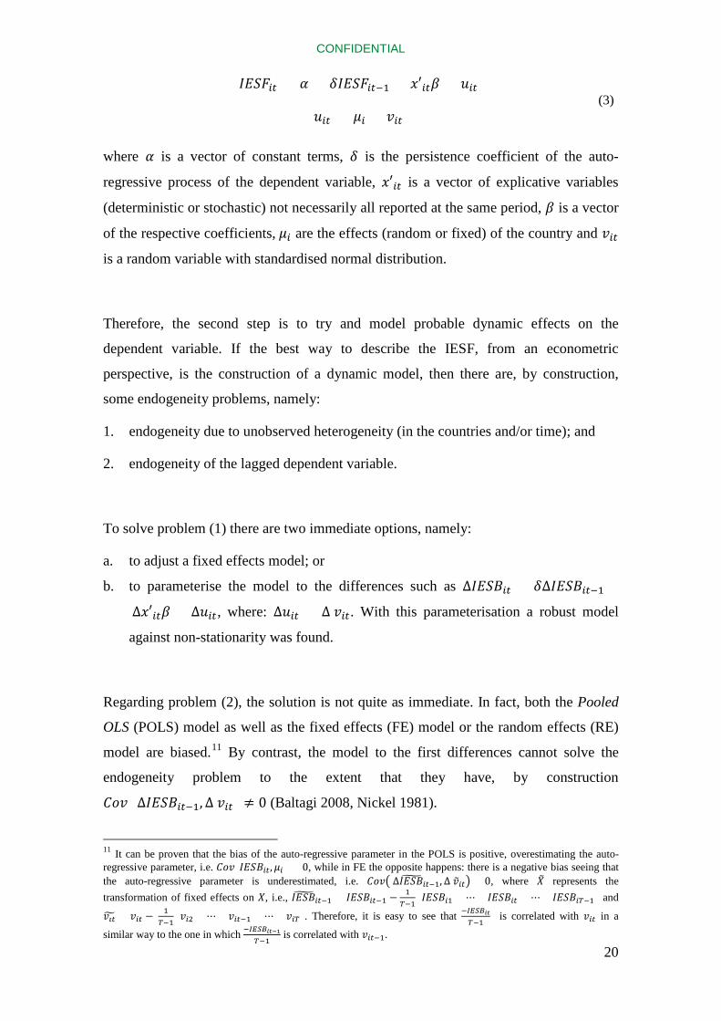
𝐼𝐼𝐼𝐼𝑖𝑖 = 𝛼 + 𝛿𝐼𝐼𝐼𝐼𝑖𝑖−1 + 𝑥′𝑖𝑖𝛽 + 𝑢𝑖𝑖

𝑢𝑖𝑖 = 𝜇𝑖 + 𝑣𝑖𝑖 (3)

where 𝛼 is a vector of constant terms, 𝛿 is the persistence coefficient of the auto-

regressive process of the dependent variable, 𝑥′𝑖𝑖 is a vector of explicative variables

(deterministic or stochastic) not necessarily all reported at the same period, 𝛽 is a vector

of the respective coefficients, 𝜇𝑖 are the effects (random or fixed) of the country and 𝑣𝑖𝑖

is a random variable with standardised normal distribution.

Therefore, the second step is to try and model probable dynamic effects on the

dependent variable. If the best way to describe the IESF, from an econometric

perspective, is the construction of a dynamic model, then there are, by construction,

some endogeneity problems, namely:

1. endogeneity due to unobserved heterogeneity (in the countries and/or time); and

2. endogeneity of the lagged dependent variable.

To solve problem (1) there are two immediate options, namely:

a. to adjust a fixed effects model; or

b. to parameterise the model to the differences such as ∆𝐼𝐼𝐼𝐼𝑖𝑖 = 𝛿∆𝐼𝐼𝐼𝐼𝑖𝑖−1 +

∆𝑥′𝑖𝑖𝛽 + ∆𝑢𝑖𝑖, where: ∆𝑢𝑖𝑖 = ∆ 𝑣𝑖𝑖. With this parameterisation a robust model

against non-stationarity was found.

Regarding problem (2), the solution is not quite as immediate. In fact, both the Pooled

OLS (POLS) model as well as the fixed effects (FE) model or the random effects (RE)

model are biased.11 By contrast, the model to the first differences cannot solve the

endogeneity problem to the extent that they have, by construction

𝐶𝑟𝑣( ∆𝐼𝐼𝐼𝐼𝑖𝑖−1,∆ 𝑣𝑖𝑖) ≠ 0 (Baltagi 2008, Nickel 1981).

11 It can be proven that the bias of the auto-regressive parameter in the POLS is positive, overestimating the auto-regressive parameter, i.e. 𝐶𝑟𝑣(𝐼𝐼𝐼𝐼𝑖𝑖, 𝜇𝑖) > 0, while in FE the opposite happens: there is a negative bias seeing that the auto-regressive parameter is underestimated, i.e. 𝐶𝑟𝑣� ∆𝐼𝐼𝐼𝐼�𝑖𝑖−1,∆ 𝑣�𝑖𝑖� < 0, where 𝑋� represents the transformation of fixed effects on 𝑋, i.e., 𝐼𝐼𝐼𝐼�𝑖𝑖−1 = 𝐼𝐼𝐼𝐼𝑖𝑖−1 −

1𝑇−1

(𝐼𝐼𝐼𝐼𝑖1 + ⋯+ 𝐼𝐼𝐼𝐼𝑖𝑖 + ⋯+ 𝐼𝐼𝐼𝐼𝑖𝑇−1) and

𝑣𝚤𝑖� = 𝑣𝑖𝑖 − 1𝑇−1

(𝑣𝑖2 + ⋯+ 𝑣𝑖𝑖−1 + ⋯+ 𝑣𝑖𝑇). Therefore, it is easy to see that −𝐼𝐼𝐼𝐼𝑖𝑖𝑇−1

is correlated with 𝑣𝑖𝑖 in a

similar way to the one in which −𝐼𝐼𝐼𝐼𝑖𝑖−1𝑇−1

is correlated with 𝑣𝑖𝑖−1.

CONFIDENTIAL

21

In short, in these circumstances of dynamic models there are two sources of persistence:

the first, which is unobserved, results from the permanent effect on the time for the

same individual and is caused by the heterogeneity term 𝜇𝑖. The second, which is

observed, occurs from the structural dependency caused by the dependency of the

dependent variable in relation to its past values (more serious the higher the value of the

autoregressive parameter 𝛿).

If, as is shown here, the problems stemming from the first persistence source are easily

solved through the estimate with fixed effects, the same cannot be said of the second, as

none of the usual models guarantee the consistency of the estimates. In fact, the logical

step relates to the parameterisation of the series to the first differences (with the

objective of removing unobserved heterogeneity) in conjunction with the method of

instrumental variables.12 Arellano and Bond ((AB), 1991)) point out past levels of series

(𝐼𝐼𝐼𝐼𝑖𝑖−𝑝 and eventually 𝑥′𝑖𝑖−𝑝) as the best solution for instrumental variables. Thus,

the AB model, which is regarded as the generalised method of moments (GMM),

consists of parameterisation of first differences to remove the endogeneity occurring

from the unobserved endogeneity in the countries where, to remove the endogeneity

occurring from the temporary persistence, the instrumental variables are past levels of

endogenous variables. However, there may be a problem with weak instrumentation

with this approach, especially when the structural persistence in time is high. For

example, one may consider, without any generality loss, a pure autoregressive model

such as:13

𝐼𝐼𝐼𝐼𝑖𝑖 − 𝐼𝐼𝐼𝐼𝑖𝑖−1 = (𝛿−1)𝐼𝐼𝐼𝐼𝑖𝑖−1 + 𝑟𝑟𝑟𝑟𝑟

If 𝛿 is close to 1 then 𝛿 − 1 will be close to zero and, therefore, the correlation between

∆𝐼𝐼𝐼𝐼𝑖𝑖 and 𝐼𝐼𝐼𝐼𝑖𝑖−1 will also be close to zero. Consequently, the instruments contain

in themselves little information on the instrumented variables; hence the consistency

and efficiency the AB model is not guaranteed.

12 These variables have to conform to two fundamental criteria: (i) to be orthogonal to the error term ∆ 𝑣𝑖𝑖 and (ii) to have relevant information on the endogenous variables (instrumented), i.e., to be correlated. 13 Subtract 𝐼𝐼𝐼𝐼𝑖𝑖−1 on both sides of the equation: 𝐼𝐼𝐼𝐼𝑖𝑖 = 𝛿𝐼𝐼𝐼𝐼𝑖𝑖−1 + 𝑟𝑟𝑟𝑟𝑟.

CONFIDENTIAL

22

A solution to this problem was proposed by Blundel and Bond (BB) (1998) who

suggested that one should use more moment conditions through system estimation.

With regard to the difference equation (as instrumented by past levels) such as the one

in the AB model, the authors suggest the addition of one equation in levels where the

instruments are the past differences of the series. In other words, the difference equation

is:

∆𝐼𝐼𝐼𝐼𝑖𝑖 = 𝛿∆𝐼𝐼𝐼𝐼𝑖𝑖−1 + ∆𝒙′𝑖𝑖𝜷 + ∆𝑢𝑖𝑖

∆𝑢𝑖𝑖 = ∆ 𝑣𝑖𝑖 (4)

where the orthogonality conditions are:

𝐼[𝐼𝐼𝐼𝐼𝑖𝑖−2∆ 𝑣𝑖𝑖] = 0

𝐼[𝒙′𝑖𝑖−1∆ 𝑣𝑖𝑖] = 0

To which an equation is added in levels:

𝐼𝐼𝐼𝐼𝑖𝑖 = 𝛼 + 𝛿𝐼𝐼𝐼𝐼𝑖𝑖−1 + 𝒙′𝑖𝑖𝜷 + 𝑢𝑖𝑖

𝑢𝑖𝑖 = 𝜇𝑖 + 𝑣𝑖𝑖 (5)

where the orthogonality conditions are:

𝐼[∆𝐼𝐼𝐼𝐼𝑖𝑖−2 𝑣𝑖𝑖] = 0

𝐼[∆𝒙′𝑖𝑖−1 𝑣𝑖𝑖] = 0

It should be noted that the equation has an over-identified model in the sense that it

contains more instruments than endogenous variables. This is the ideal condition

because if one enjoys more moment conditions, one significantly improves the results in

terms of consistency and efficiency. Thus, one cannot exactly satisfy the orthogonality

conditions in the sense that they are equalled to zero because the matrix which is the

result of the product of the matrix of regressors by the matrix of instruments is not a

square matrix, therefore it is not invertible. The intention of the GMM is to meet as

many of the moment conditions as possible, therefore minimising the distance between

the orthogonality conditions. This is the method that will be used in the estimation of

the AB and BB models.

CONFIDENTIAL

23

It is important to specify the variables that were tested to be used in the model, such as

the selected group of variables used, i.e., how vector 𝑥𝑖𝑖′ was built. In this regard, the

explanatory variables can be grouped in two distinct groups. In the first group – the

vector 𝑥1𝑖𝑖′ – there are variables that refer to the countries’ specific indicators; therefore,

they assume distinct values from country to country. This group is formed by the

variables [𝑚_𝑦𝑖,𝑖;𝑐𝑐𝑟𝑟𝑟𝑖,𝑖; 𝜋𝑖,𝑖; 𝑟𝑟𝑟𝑖,𝑖], where:

• 𝑚_𝑦𝑖,𝑖, given by the ratio of M2 to nominal GDP, measuring the degree of

monetisation of the economy, is an adequate means to assess the development, the

depth and dimension of the financial sector (Outreville 1999);14

• 𝑐𝑐𝑟𝑟𝑟𝑖,𝑖 is the current account balance to GDP ratio, providing a measure of

external performance;15

• 𝜋𝑖,𝑖 is the year-on-year inflation rate given by a 12-month change in the CPI of each

economy; and

• 𝑟𝑟𝑟𝑖,𝑖 is the annual change of the international reserves. It is an indicator of the

external solvency of each economy, i.e., of the capacity that each central bank has

to mitigate external shocks.

Control variables were inserted nn the second group – vector 𝑥2𝑖𝑖′ . One should note that

the variables related to the global macroeconomic environment that do not change

between countries. The selected variables were the annual change of the oil price, 𝑐𝑖𝑜,

and the GDP real growth of the G2016 (𝑔𝑤𝑖).

14 According to Carlin and Soskice (2006), M2 corresponds to M1 (the financial assets that perform the function of immediate means of payment: currency in circulation, deposits on call and the like) and the highly liquid financial assets which, although they are not immediate means of payment, adequately comply with the remaining monetary functions (namely the store of value). By contrast, it is the only one in respect of which there is available data for the period under review. 15 The use of this indicator, as it will be seen later, is very significant and it means another set of indicators which could also have been relevant should be left out of this panel. Examples include the price of international commodities with an evolution which may be relevant for external accounts, the use of the exchange rate which may give an indication of the level of competitiveness, or the growth of the economy in view of the fact that for the majority of the economies in the region the economic growth is strongly linked to the export sector. 16 The G-20 group is formed by South Africa, Argentina, Brazil, Mexico, Canada, United States, China, Japan, South Korea, India, Indonesia, Saudi Arabia, Turkey, European Union, Germany, France, Italy, Russia, United Kingdom and Australia.

CONFIDENTIAL

24

As for the model estimation, the starting point went through the recourse to standard

methodologies, namely POLS, the FE model and the RE model.17 In relation to this

point, some observations stand out, namely:

1. there are peculiar fixed effects in the countries;

2. there are dynamic effects;

3. theoretical results relating to the inconsistency of the above-mentioned

appreciators are confirmed empirically: POLS tends to overestimate the

autoregressive parameter, while the FE model tends to underestimate it; and

4. the estimate of the autoregressive parameter given by the BB methodology is

lower than the one obtained by POLS, but is higher than the one obtained

through the FE model. Such an occurrence is totally in accordance with what

could be expected. In fact, as it was previously argued, insofar as a consistent

estimate for the autoregressive parameter was limited by the estimates of POLS

and the FE model. This circumstance is a characteristic of the consistent results

that the BB model produces.18

The estimate was carried out using Stata software and, in particular, with the help of the

xtabond2 package (Roodman 2009a). Due to the problem of the weakening of the

Hansen tests in the presence of the proliferation of a number of orthogonality

conditions, the instruments matrix was collapsed (Roodman 2009b).

In both the AB and BB models, the two-step GMM with bias was also considered

(Windmeijer, 2005). There are some differences between the BB and AB estimates with

respect to the autoregressive coefficient. Besides, this is an expected result given that

methodology’s propensity for underestimating this parameter. This situation proves,

once again, the quality of the BB model in the context addressed. Therefore, given the

high persistence of IESF over time, the correlation between the differences and past

levels is significantly reduced. As a result, the past levels of the series do not effectively

fulfil their function of implementing the lagged dependent variable (which is

endogenous by construction) because, as such, they have little information on the

17 Testing the presence of fixed effects on individuals, the null hypothesis of fixed effects’ redundancy was rejected at a level of nominal significance inferior to 1 per cent. To note that in this model, the temporal fixed effects were not considered. Neither temporal dummies nor trend terms (which impose the restriction of equality of temporal dummies) were certified as significant variables. 18 In practice, this situation is not always the case, following the idea that the theoretical and empirical results can sometimes be very divergent.

CONFIDENTIAL

25

variable to be implemented and therefore there is a problem of weak instruments. The

probability that, from the modulation skills, the same occurs with the remaining

explanatory variables should be noted. Consequently, this is one more excellent

indication of the system of Blundell and Bond.

Lastly, regarding diagnostic tests, it is important to mention two fundamental issues:

1. Arellano and Bond autocorrelation tests apply where the null hypothesis is one of

the absences of autocorrelation of the first and second order:

�𝐻0:𝐼[𝛥𝑢𝑖𝑖𝛥𝑢𝑖𝑖−1] = 0𝐻1:𝐼[𝛥𝑢𝑖𝑖𝛥𝑢𝑖𝑖−1] ≠ 0

and

�𝐻0:𝐼[𝛥𝑢𝑖𝑖𝛥𝑢𝑖𝑖−2] = 0𝐻1:𝐼[𝛥𝑢𝑖𝑖𝛥𝑢𝑖𝑖−2] ≠ 0

2. Hansen tests and Hansen differentials validate the instruments identified above.

These tests aim to give

(i) a global validity of the instruments, (ii) the validity of the instruments of the

predetermined and/or endogenous variables and (iii) the validity of the instruments

of the variables considered to be strictly exogenous which, in this case were a

deterministic linear trend, the oil price and global growth.

5. Empirical estimation

5.1 Stability indicator

Based on the methodologies presented in the section above, Figure 7 shows the IESF

obtained for each SADC Member State. The sample covers the period 2008–2014,

except for Botswana, the DRC and Lesotho, which are covered until 2013 due to data

availability.

CONFIDENTIAL

26

Figure 7: Financial sector stability index

10

20

30

40

50

60

2008 2009 2010 2011 2012 2013 2014

Angola

10

20

30

40

50

60

70

2008 2009 2010 2011 2012 2013

Botswana

0

20

40

60

80

100

2008 2009 2010 2011 2012 2013 2014

Democratic Republic of the Congo

0

20

40

60

80

2008 2009 2010 2011 2012 2013

Lesotho

10

20

30

40

50

60

2008 2009 2010 2011 2012 2013 2014

Madagascar

0

20

40

60

80

100

2008 2009 2010 2011 2012 2013 2014

Malawi

10

20

30

40

50

60

70

2008 2009 2010 2011 2012 2013 2014

Mauritius

10

20

30

40

50

60

70

2008 2009 2010 2011 2012 2013 2014

Mozambique

0

20

40

60

80

2008 2009 2010 2011 2012 2013 2014

Namibia

20

30

40

50

60

70

80

2008 2009 2010 2011 2012 2013 2014

Seychelles

10

20

30

40

50

60

2008 2009 2010 2011 2012 2013 2014

South Africa

10

20

30

40

50

60

70

2008 2009 2010 2011 2012 2013 2014

Swaziland

0

20

40

60

80

2008 2009 2010 2011 2012 2013 2014

Tanzania

10

20

30

40

50

60

70

2008 2009 2010 2011 2012 2013 2014

Zambia

0

20

40

60

80

100

2008 2009 2010 2011 2012 2013 2014

IESF MEAN

Zimbabwe

Note: Calculations made by the authors. The data were obtained from the region’s central banks and from the IMF.

A sample starting in 2008 was considered as this is the year that marks the beginning of

the turmoil experienced in the global financial markets, followed by a slow global

recovery in subsequent years. In this way, the indicators are able to capture an important

sample, therefore becoming very informative.19

The study shows that there was a break in the soundness of the banks in most

economies during 2009 and 2010, such as Angola, Botswana, DRC, Lesotho,

Madagascar, South Africa, Tanzania and Zambia. For example, in Angola, 2010 was the

19 The information presented at the end of this chapter was supplied by the central banks of the SADC countries. For a more complete characterisation, please consult Annex 1.

CONFIDENTIAL

27

year with the lowest point in financial stability due to high levels of non-performing

loans (including write-offs) and low solvency levels.20

Nevertheless, until 2013, it appears that the financial stability of Angola, Madagascar,

Mauritius, Mozambique and Zimbabwe followed a downward trend. Therefore, the

credit risk of the countries increased, mainly for Angola and Madagascar. At the same

time, there were substantial declines in capital profitability, with the exception of

Madagascar whose economy has been hit by an economic crisis since 2009.

Zimbabwe also merits special mention in that it had unfavourable developments in all

dimensions of the constructed index. It should be noted that this country’s major

difficulties are liquidity constrains, a low amount of new deposits, limited foreign

lending facilities and the companies’ low economic viability. In addition, the rigidity of

the microstructure, such as transitory deposits, and the absence of an active interbank

market culminated in the gradual rise of overdue loans, liquidity, recapitalisation and

low profitability in some banking institutions.

By contrast, in the group of countries that registered a stable position around the mean

of their financial environment are DRC, Lesotho, South Africa and Seychelles,21

explained for the most part by the strength of their banking system regulatory and

operational framework. In the case of Seychelles, despite the index drop in 2012, the

sample showed a broadening of the banking sector accompanied by the introduction of

new legislation to promote and support the stable development of this sector.22 In the

specific case of South Africa, given its relevant international participation, there was

also a review and alteration of the banking-sector legislative and regulatory framework

to ensure a framework in compliance with international regulatory standards.23

20 It is important to mention that 2010 is also associated with the significant increase in the central government’s net credit to, among others, comply with accumulated late payments to foreign capital institutions, thus creating a downstream chain of postponements and nonfulfillment of those state duties (Banco Nacional de Angola, 2013). 21 Due to the forced financial liberalisation of the 1980s and 1990s, serious macroeconomic imbalances were registered. However, a continuous improvement of the financial sector was witnessed, resulting from the reforms agenda of those two decades meant to reinforce the levels of solvency and risk management (Mlachila, Park and Yaraba, 2013). 22 The list of legislations introduced may be obtained at http://www.cbs.sc/Legislations/cbsact.jsp. 23 South Africa implemented Basel II, effective from 1 January 2008. The implementation implied among others, a radical change in disclosure methodology, reviewed regulatory returns and a better alignment of

CONFIDENTIAL

28

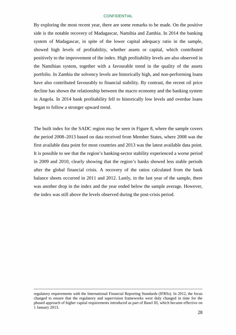
By exploring the most recent year, there are some remarks to be made. On the positive

side is the notable recovery of Madagascar, Namibia and Zambia. In 2014 the banking

system of Madagascar, in spite of the lower capital adequacy ratio in the sample,

showed high levels of profitability, whether assets or capital, which contributed

positively to the improvement of the index. High profitability levels are also observed in

the Namibian system, together with a favourable trend in the quality of the assets

portfolio. In Zambia the solvency levels are historically high, and non-performing loans

have also contributed favourably to financial stability. By contrast, the recent oil price

decline has shown the relationship between the macro economy and the banking system

in Angola. In 2014 bank profitability fell to historically low levels and overdue loans

began to follow a stronger upward trend.

The built index for the SADC region may be seen in Figure 8, where the sample covers

the period 2008–2013 based on data received from Member States, where 2008 was the

first available data point for most countries and 2013 was the latest available data point.

It is possible to see that the region’s banking-sector stability experienced a worse period

in 2009 and 2010, clearly showing that the region’s banks showed less stable periods

after the global financial crisis. A recovery of the ratios calculated from the bank

balance sheets occurred in 2011 and 2012. Lastly, in the last year of the sample, there

was another drop in the index and the year ended below the sample average. However,

the index was still above the levels observed during the post-crisis period.

regulatory requirements with the International Financial Reporting Standards (IFRSs). In 2012, the focus changed to ensure that the regulatory and supervision frameworks were duly changed in time for the phased approach of higher capital requirements introduced as part of Basel III, which became effective on 1 January 2013.

CONFIDENTIAL

29

Figure 8: Global financial sector stability index

20

25

30

35

40

45

50

55

60

2008 2009 2010 2011 2012 2013 2014

IESF Mean Mean-1SD Mean+1SD Note: Calculations done by the authors. The data were obtained from the central banks of the region and the IMF.

5.2 Determinants

Table 2 shows the results relating to the POLS, EF, AB and BB models. The models

used quarterly data for the period 2008–2013 for all SADC Member States with the

exception Swaziland due to some data problems.

When interpreting the coefficients, it is important to mention that a negative relationship

between the degree of financial deepening and the financial stability of the banking

system is observed. This outcome is somewhat expected, as financial deepening implies

a more sophisticated financial system or a more leveraged one, which can certainly

increase the probability of risk materialising as the banks become more exposed to

them. It is important to note that Dell’Ariccia (2006) showed empirical evidence of a

trade-off between financial deepening and financial stability. However, there is another

point to ponder: when discussing less developed financial systems such as those of most

SADC economies, more financial deepening may indicate an environment that is more

favourable to financial intermediation. This can result in the banks’ profitability and

also an improvement in credit risk by virtue of it being easier to get resources to ensure

compliance with debt servicing in deeper financial systems. But what was empirically

established was that, taking into consideration the indicators that make up the IESF, the

theoretical negative effects outweighed the theoretical positive effects.

CONFIDENTIAL

30

Table 2: Results from estimates of the static and dynamic GMM models

Pooled OLS Fixed effect Arellano and Bond

Blundell and Bond

No. of observations 315 315 301 315 No. of groups 14 14 14 14

No. of instruments … … 133 140 F( 9; 14) 314,53*** 1247,99*** … …

R2 0,7377 0,6971 … … Wald χ2 (9) … … 617,70*** 684,14***

Exogenous variables Coeficient1) Coeficient1) Coeficient2) Coeficient2)

𝑰𝑰𝑰𝑰𝒕−𝟏 0,8306*** (1,01)

0,7384***

(16,28) 0,7392***

(16,28) 0,7850* (19,04)

𝒎_𝒚𝒕 -0,0121

(1,01) -0,0576 (16,28)

-0,1666** (-2,53)

-0,1015* (-2,05)

𝒄𝒄𝒄𝒄𝒄𝒕 0,0346

(1,01) 0,1766**

(16,28) 0,2569***

(4,07) 0,2420***

(3,50)

𝒑𝒕𝒄 -0,0383 (1,01)

-0,0381 (16,28)

-0,0521*** (-2,87)

-0,0523*** (-2,34)

𝝅𝒕 -0,2063*

(1,01) -0,2167*

(16,28) -0,1731*

(-1,90) -0,1939**

(-2,23)

𝝅𝒕−𝟏 0,2140*** (1,01)

0,1566* (16,28)

0,1994*** (2,21)

0,2613*** (2,32)

𝒄𝒓𝒓𝒕 -0,0011

(1,01) -0,0016 (16,28)

-0,0017 (-1,1)

-0,00067 (-0,34)

𝒄𝒓𝒓𝒕−𝟏 0,0012* (1,01)

0,0007 (16,28)

0,0003 (0,18)

0,0001 (0,48)

𝒈𝒈𝒕 0,3132

(1,01) 0,0704 (16,28)

0,3359 (1,01)

0,4402 (1,30)

C 6,1063* (1,01)

14,1406** (16,28) … 12,665***

(3,41) 1) The t-statistic ratio is inside the brackets 2) The z-statistic ratio is inside the brackets

Note: The exponent * indicates statistically significant at 1 per cent, while ** indicates statistically significant at 5 per cent.

However, the variable current-account balance as a ratio of GDP is highly significant,

which indicates that the better the external performance in explaining economic growth,

the better the contribution towards stability of the banking sector. A possible

explanation for this result could be attributed to the evidence that the exporting

companies’ activity is supported by the banking sector. In this way, when there is a

deterioration in the current account, the economy’s exporting sector is not sufficiently

competitive to increase its revenue, and given the exposure of the banks to the sector,

the profitability and credit risk may undermine the sector’s stability and resilience.24

24 It is important to mention that a big weight of the lending activity in most of the countries under review is aimed at the exporting companies instead of being directed to the households; hence the stability of the exporting sector can be seen as a cornerstone interlinking the macroeconomic environment and the financial sector.

CONFIDENTIAL

31

As might be expected, inflation also has a negative effect on the stability of the banking

sector. In order to maintain positive real profitability, the banks would have to raise

interest rates, which may contribute positively to the banks’ profitability. But this may

hamper the agents in complying with their contractual obligations, which would in turn

create negative consequences for the capitalisation of the institutions. In addition, this

result is consistent with the current-account result, because higher inflation makes the

exporting companies lose their competitiveness and thus there is a deterioration in the

current account.

In terms of the oil price, there is a negative causal link for financial stability. It should

be noted that Angola is the only country considered to be a large oil exporter in SADC,

while the remaining countries, despite some being oil exporters on a smaller scale, are

clearly oil-importing countries. Because oil is an almost irreplaceable input in the

production and logistics process, a rise in its price could have a negative impact on the

profitability of companies and, consequently, create difficulties to the banks exposed to

such companies. Proof of the robustness of the results obtained is to associate the oil

coefficient with the inflation and current-account coefficients, i.e., an increase in the oil

price can positively influence inflation and negatively influence the current account.

Lastly, it is important to mention the statistical and economic significance of the lagged

dependent variable. In fact, the autoregressive parameter 𝛿 is statistically different from

zero, which suggests the existence of structural persistence in financial stability. From

the viewpoint of economic rationality, this circumstance implies that a period of

(in)stability at present will tend to be followed by periods of (in)stability in the future.

Consequently, the recommendations from the systemic risk analysis are of a forward-

looking nature, i.e., it is not sufficient to evaluate the system when risks are

materialising; instead, one should act to prevent them from materialising as financial

stability may spiral out of control. Table 3 summarises the results of these diagnostic

tests.

CONFIDENTIAL

32

Table 3: Diagnostic of the Blundell and Bond model

Arellano-Bond autocorrelation test for differential model

Test Z p-value

AR(1): first order -4,6*** 0,000

AR(2): second order -0,35 0,724

Validation of the over-identified moment conditions

Hansen tests Degrees of

freedom: n χ2

p-value

Global 130 135,20 0,360

Hansen differential tests for equations in levels and to the differences

Predetermined and endogenous variables 123 121,69 0,517

Strictly exogenous variables 129 135,20 0,337

1) Exogeneity test of the instruments subgroup: GMM instruments for level series. The signs *;** and *** indicate statistical significance at 10 per cent, 5 per cent and 1 per cent respectively.

Regarding Arellano and Bond’s autocorrelation tests, it should be mentioned that, by

construction, the errors follow the AR(1) process. Algebraically, ∆𝑢𝑖𝑖 = (𝜇𝑖 + 𝑣𝑖𝑖) −

(𝜇𝑖 + 𝑣𝑖𝑖−1) = 𝑣𝑖𝑖 − 𝑣𝑖𝑖−1 = ∆𝑣𝑖𝑖. It follows that, not only is it normal, but that the

first-order autocorrelation in the errors is also positive. More positive still is the fact that

there is evidence of the absence of autocorrelation of the order larger or equal to 2, since

it is the true test of autocorrelation.

The Hansen tests verify the validity of the over-identified moment conditions, i.e., if the

instruments perform their function correctly and if the endogeneity problems are

resolved. In fact, there is empirical evidence, not only of the validity of the equation’s

variables in levels but also in first differences. Furthermore, 𝑐𝑖𝑜 and 𝑔𝑖,𝑖 are seen as

predetermined variables,25 while the remaining are endogenous variables. Such

reckoning is correct, or at least in accordance with what is required, as long as the null

hypothesis of the instruments’ invalidity cannot be rejected.

In short, the variables’ exogeneity nature was correctly specified. It should be noted that

the choice of the variables’ nature is not given by the economic theory, but it emerges

from the model itself, which derives from letting the data speak.

25 It should be noted that an exogenous variable in the levels’ equation will be predetermined in the differences equation, that a predetermined level’s variable will be endogenous to the differences. Therefore there is a need to carry out predetermined variables.

CONFIDENTIAL

33

6. Complementary analysis

During the course of this work, the paper debated the idea that the balances of the banks

in SADC countries are mainly influenced by variables of a macroeconomic nature, and

that those balances respond, in a heterogeneous manner, to shocks in macroeconomic

aggregates. In fact, as it was verified throughout this work that the SADC economies

display a heterogeneous behaviour due to the unique characteristics of each of the

region’s Member States and, consequently, the same applies to the balances of each

Member State.

It is in line with this idea that in this section three complementary analyses will be dealt

with to support the cross-disciplinary of this attempt. In particular, countries will be

dealt with individually for the purpose of: (i) analysing the bilateral financial

relationships between the countries and the outside world; (ii) identifying clusters in the

region’s financial systems; and (iii) performing a comparative analysis between

countries, taking into account their economic and financial stability.

6.1 Cluster analysis

The aim of this sub-section is to identify similarities and differences among the

countries in the SADC region by way of a cluster analysis. After having selected the

indicators (see Table 4), they were standardised to present them in the same scales,

which assists with the implementation of the cluster analysis methodology for ease of

interpretation. The selection of the indicators took into consideration the theoretical and

conceptual aspects relating to the financial systems’ generalities.

The indicators that seek to capture the structure of the region’s financial systems take

into account:

i. macroeconomic factors that can affect the search for banking services and reduce

the risks associated with their offer;

ii. ratios of the banks’ balances;

iii. indicators of financial inclusion;

iv. spread of the banks’ lending and deposits interest rates;

v. macroprudential indicators; and

vi. structural indicators related to the financial-sector structure.

CONFIDENTIAL

34

Table 4: Indicators for use in the clusters

Macroeconomic factors

Year-on-year inflation

Real growth of GDP

Current account (per cent of GDP)

Exchange rate (year-on-year change)

Net foreign direct investment (per cent of GDP)

Pricing indicators

Spread between lending and deposit interest rates

Financial structure

Credit to the private sector (per cent of GDP)

M2 (per cent of GDP)

Macroprudential indicators

M2/total reserves

Credit to private sector (per cent of GDP) gap

Financial inclusion

Number of banking branches per 100 000 adults

Number of ATMs per 100 000 adults

Macroprudential indicators

Capital adequacy

Performing loans

Return on assets

Return on equity

Furthermore, with regard to the methodology, after the definition of data matrix and its

standardisation26 as a measure towards the distance between the systems in the regions,

it was decided to use the squared Euclidean distance, as in the cluster building process,

the distinction between them is made in accordance with the more heterogeneous

financial systems. This approach is followed by Wolfson (2004) and Sorensen et al.

(2006).

The cluster process selected was the hierarchical clustering algorithm because it allows

the grouping of similar banking systems without specifying ex ante a pre-established

26 The standardisation method for this cluster exercise involves considering the deviations vis-à-vis the duly weighted averages by the standard deviation. This ensures that all the variables have a null average and unitary variation.

CONFIDENTIAL

35

number of clusters. The algorithm’s underlying technique relies firstly on placing each

system in a distinct group. Next, each system is incorporated into successfully bigger

groups, as per the cluster method chosen. This exercise uses the complete linkage

method which joins two clusters characterised by the greater distance between any two

objects in the different groups, i.e., the further clusters.

In order to identify the clusters by way of the explained methodology, it was intuitive to

use a dendrogram. Using this map, the heterogeneity already mentioned could be

proven and various groups could be identified. Furthermore, this type of illustration also

assists with the interpretation of the proximities between the countries given the

indicators used. The dendrogram of this analysis is shown in Figure 9.

Interpreting the picture is easy and quite intuitive. For example, if the SADC region is

divided into three groups/clusters, having as a reference the distance of 7, then the order

would be, from right to left, South Africa, Mauritius, Swaziland, Seychelles, Namibia,

Lesotho and Botswana in a group; Malawi alone in the middle group; and the rest of the

countries would be in another cluster, more to the left.

CONFIDENTIAL

36

Figure 9: Dendrogram for cluster analysis

Sources: IMF, World Bank and SADC central banks. Calculations were done by the DES/BNA.

However, if the links between the countries are deepened, using the distance of 5 as a

reference, six distinct clusters can be identified and interpreted. One group is formed by

the DRC, Zambia, Tanzania and Mozambique. Angola appears separately in the second

cluster. Cluster 3 includes Madagascar and Zimbabwe. Malawi is alone in the fourth

group. A fifth group is constituted by Namibia, Lesotho, Botswana, Swaziland and

Seychelles. Lastly, there is a group comprising Mauritius and South Africa. The clusters

identified are organised in Table 5.

Table 5: Identification of clusters for the homogeneity of the banking sector, 2013

Cluster Frequency Countries Percentage

1 4

Zambia DRC

Tanzania Mozambique

26,67

2 1 Angola 6,67

3 2 Madagascar Zimbabwe

13,33

4 1 Malawi 6,67

5 5

Namibia Botswana Lesotho

Swaziland Seychelles

33,33

6 2 South Africa

Mauritius 13,33

Total 15 100

02

46

810

Dis

tanc

e

AGOCOD

TZAZMB

MOZMDG

ZWEMWI

BWALSO

NAMSYC

SWZMUS

ZAF

Country

CONFIDENTIAL

37

Concerning the proximity of the countries’ financial systems and taking into account the

indicators used, in first place is Tanzania and Zambia, followed by Lesotho and

Botswana. It should be noted that inside the clusters identified with more than one

country, the cluster comprising South Africa and Mauritius (cluster 1) is the group with

the highest general homogeneity of the selected indicators among the countries,

followed by cluster 2 which comprises the DRC, Zambia, Tanzania and Mozambique.

The proximity between Mauritius and South Africa is intuitive due to the structural

factors of their financial systems. It is important to note that in Africa, both countries

are reference countries when it comes to the role of financial intermediation and

financial deepening of their economies.

With regard to the DRC, Zambia, Tanzania and Mozambique, one common

characteristic is identifiable in those countries and has to do with the fact that in the

region they are the richest countries in terms of natural resources. As argued by Cabello

et al. (2013), this characteristic means that these banking systems have negative net

external positions, partly due to the presence of large foreign extractive companies.

Mozambique is the least homogeneous country in this cluster, probably due to the

economy’s relative net foreign direct investment (FDI).

Although Angola could also belong to cluster 1, due to its characteristic wealth of

natural resources it was isolated due to the contribution that its first natural wealth (oil)

has on the economy. Also, this country is the only country with a net lending position in

the international investment.

With regard to Zimbabwe and Madagascar, in spite of their inclusion in the same

cluster, the distance between their financial systems is relatively vast. This is due to the

high level of non-performing loans and interest rate spreads that exist in Madagascar,

which are the highest in the region. However, concerning the other indicators, the

countries show some proximity which contributed to their integration into a single

cluster.

CONFIDENTIAL

38

Malawi’s banking system is the one that emerges as the least integrated in the region,

which resulted in its isolation in a cluster. This is, understandably, due to the high

inflation rates and exchange rate depreciation for the period under review.

Lastly, in relation to cluster 5, with the exception of Seychelles, all the countries,

including Namibia, Lesotho, Botswana and Swaziland, are formally linked to South

Africa. It should be mentioned that the countries that form part of the Common

Monetary Area (CMA) are South Africa, Namibia, Lesotho and Swaziland.

Furthermore, Botswana, together with the CMA countries, constitutes the Southern

African Customs Union (SACU). The exclusion of South Africa from this cluster has to

do with the financial system’s structural factors. The introduction of Seychelles into this

cluster is due to the general homogeneity of the indicators used. Nevertheless, it is

important to mention that this cluster can be divided into two sub-clusters, including in

one first group Namibia, Botswana and Lesotho, and in the second group Swaziland and

Seychelles.

6.3 Network approach

Both the econometric study and the clusters approach were limited to the SADC

economies. It is important to understand the channels through which situations of

contagion and transmission of the world system’s geopolitical instability occur in the

SADC region. One of the more immediate approaches for monitoring banking-sector

risk deals with observing the international exposure level. The networking perspective

allows for this ensuring that it outlines the bilateral relations of lending among the

countries under review. An indicator that measures bilateral financial exposure with

another is given by the ratio between assets vis-à-vis a country in relation to the total

assets portfolio.

Starting from a more inclusive sample, correspondences regarding the international

exposure of the economies were selected in order to better understand the environment

involved in the international exposure of the countries. For this purpose, the study used

cross-sectional data for SADC countries for 2012. During map preparation, some

CONFIDENTIAL

39

aspects regarding country selection and their respective interrelationships were taken

into account, for example:

1. Data made available by the SADC central banks, especially regarding South Africa,

Angola, Seychelles, Namibia and Zimbabwe.

2. When it was not possible to obtain the categorised data from some of the central

banks, the study used the amount of liabilities from South Africa to obtain the

bilateral relationship with this country.

3. For the economies outside the region data was sourced from the BIS27 database. For

investment recipients only the exposures relevant for this specific map were

considered. The introduction of Portugal is due to the strong exposure of Angola to

this country, with more than 50 per cent of its international assets being destined to

Portugal. The introduction of United Kingdom (UK), US and Germany is due to the

exposures of the countries in the region to them. For example, more than 50 per

cent of South Africa’s international assets are destined to the US and the UK. In

Zimbabwe, approximately 70 per cent of the international assets originate in the

US, while in the Seychelles around 80 per cent of the assets are in the UK.

4. Bilateral relations were also considered among the SADC countries whenever these

were higher than 2 per cent. Figure 10 shows the networking built from the

simplifications presented above.

Figure 10: Internationalisation of the SADC banking systems from a network perspective

Source: Central banks of the SADC countries; Bank for International Settlement; calculations carried out by the authors of the document. The exposure of Lesotho is calculated indirectly by way of the foreign originated liabilities, broken down by countries, from South Africa and from the total international assets supplied by Lesotho.

27 Database available at http://www.bis.org/statistics/consstats.htm

CONFIDENTIAL

40

Note: The thickness of the line corresponds to the concentration of the bilateral exposure in terms of the international assets of a banking system. The black dotted lines correspond to a bilateral exposure ratio between countries in the region, higher than 2 per cent and less than 9 per cent.

In general, inside this network, the US and UK are two financial centres whose

developments should be followed closely by the SADC region. Furthermore, South

Africa is the main destination of the investment from the countries in the intra-SADC

region. Thus, an interpretation of this network shows that moments of bigger financial

weakness in the US and UK may lead to:

1. an intensification of the weaknesses of those countries through their strong

relationships;

2. a harmful contagion among other countries exposed internationally due to them

being two financial centres of great importance worldwide.28 In the network

example, Germany is exposed to both countries and is a destination with some

weight regarding the investments from Zimbabwe and Angola;

3. problems in the SADC countries with a high direct exposure to those countries,

for example, Zimbabwe, Namibia and Angola to the US; Seychelles to the UK;

and South Africa to both; and

4. problems with countries in the region with high exposure to South Africa, for

example, Lesotho or Namibia.

Due to the relatively low proportion of their international asset portfolio with the total

assets, the banking systems in SADC do not appear dogged by solvency problems, even

in a very pessimistic scenario. However, it is very probable that losses occur in the

South African financial system associated with its international exposure due to the

more developed features of its financial system.

It is important to mention that, although most of the financial systems in the SADC

Member States are still at a less developed stage, some countries are particularly

sensitive to events in South Africa. For example, due to the exchange rate parity, the

developments of South Africa’s financial and foreign-exchange market may also affect

28 Another example that for reasons of simplification was not shown in the network has to do with the exposure of Portugal to Spain and of Spain to the US. Given the high exposure of Angola to Portugal, problems in the US would affect Angola, not only due to its direct exposure to the US, but also via its indirect exposure via Portugal. In the network another indirect exposure is also visible, via Germany.

CONFIDENTIAL

41

the CMA countries. Furthermore, Botswana, which together with other CMA countries

belongs to SACU, is also affected due to its strong trade relations with South Africa and

the exchange rate regime of a crawling peg.

Apart from this, the rationale underlying the network analysis refers to the fact that the

analysis cannot be static and direct. Thus, by accumulating a set of impacts from the

various scenarios defined in points 1 to 4, the exposure of the SADC financial systems

may weaken relative to the global scenario. In this way, prudential regulation directed at

limiting the concentration of financial systems’ exposures in some countries could be a

point to take into account in the SADC agenda. Some factors to consider within this

topic could be linked to stipulating maximum direct and indirect limits of exposure to

certain countries, or the obligation for banks to provide a threshold of the total of their

international investments so that in a worst-case scenario any eventual future loss on

their investments is already accounted for and will not impact the financial stability

ratios.

6.3 Comparative analysis between countries

This section proposes a methodology to identify which countries have higher levels of

economic and financial vulnerability. The methodology used is similar to the one used

to calculate the IESF. However, instead of making a temporal analysis by country, the

data was compiled by period between countries. In other words, the approach is similar

to the one used by the United Nations Development Programme (UNDP) for the

calculation of some development indexes.

The indicators associated with financial inclusion and the FDI are derived from the

indicators used in the cluster, complementing them with the remaining macroeconomic

convergence indicators used. Table 6 summarises the indicators used and the sign

assigned to that indicator according to the theoretical positive or negative correlation

with the risk.

CONFIDENTIAL

42

Table 6: Selected indicators for financial and economic stability (cross-section, 2013)

Macroeconomic factors

Year-on-year inflation (-)

GDP real growth (+)

Current account (per cent of GDP) (+)

Year-on-year change of exchange rate (-)

Budget balance (per cent of GDP) (+)

Public debt (per cent of GDP) (-)

Months of imports cover (+)

Pricing indicators

Spread between lending and deposit interest rates (-)

Financial structure

Credit to the private sector (per cent of GDP) (-)

M2 (per cent of GDP) (-)

Macroprudential indicators

Credit to private sector (per cent of GDP) gap (-)

Microprudential indicators

Capital adequacy (+)

Non-performing loans (-)

Return on assets (+)

Return on equity (+)

The purpose of building the indicator was to identify the countries that, in 2013, had

more vulnerable economic and financial situations. The difference between this new

indicator and the IESF calculated in Section 4 is that the latter allows the comparison of

the financial-sector stability level of a country for the historical sample used. By

contrast, the indicator built in this subsection enables a comparison of the stability of the

financial sector and economies of the countries in the sample for a certain period. For

2013, the countries’ indicator in terms of global stability, i.e., financial sector and

macroeconomic stability, is shown in Figure 11.

CONFIDENTIAL

43

Figure 11: Financial and economic stability index (cross-section, 2013)

Source: SADC central banks and the World Bank. Calculations carried out by DES/BNA

What can be observed is that South Africa and Mauritius had the lowest levels of

financial and economic stability for 2013. It is important to note that these two countries

share the same cluster, mainly due to the high levels of financial deepening observed,

much higher in general than the remaining economies. The variable financial and

economic stability index was tested in the econometric model and was significant and

negatively related to the stability of the IESF. Moreover, as the two financial systems

are internationally dynamic, in particular South Africa, it can be concluded that this

cluster should be further modernised. This study reinforces the arguments of Cabello et

al. (2013) that suggest that cross-border supervision in the region is a topical issue. This

author mentions some of the prominent banks in South Africa whose exposure to the

rest of the African continent is seen as a warning, such as Standard Bank and Ecobank.

7. Final remarks and policy recommendations

This study aimed to discuss financial stability in SADC economies in an innovative and

trans-disciplinary manner. The contribution to the literature includes the application of

methodologies that are usually reserved for the so-called developed economies.

SADC financial stability was split into two major areas, namely macroeconomic

stability and banking-sector stability. The study examined the extent to which a set of

exogenous variables contribute to financial stability of the Member States in the region,

particularly variables common to all and unique variables.

CONFIDENTIAL

44

It was shown that the economic and financial indicators were proven to be quite

heterogeneous from country to country, and that realisation took place in all the

exercises carried out in the document.

An IESF was created and it grouped four ratios of the banks’ balance sheet, which were

used as proxy to banking stability. Furthermore, the high persistence of the built index

was revealed, which was shown in two manners: through the latent heterogeneity and a

dynamic that characterised it. The first source of persistence was treated, including fixed

effects in the sectional units and, in turn, the second source of persistence, the dynamic

persistence, was modelled using an estimate system following the methodologies of

Blundell and Bond.

The variables that contribute the most towards explaining the created index are the

inertia factor of financial stability, the degree of financial deepening (ratio of M2/GDP),

the current-account ratio of GDP, the inflation rate and the oil price.

Given the high statistical significance of the current-account balance, it is advisable to

think of a programme structured to stimulate the competitiveness of the region’s

economies. Such recommendation is encouraged in this case for stability in the banking

sector and because it is in line with two criteria of SADC’s economic convergence,

namely the inflation rate and economic growth.

An important factor to consider relates to the negative sign of the financial deepening

coefficient. In fact, the characteristics of the region’s financial systems are reflected, in

general and when compared with benchmarks from other regions, in a reduced banking

level, a little diversified business model, a low degree of financial deepening and a well-

capitalised system. Such characteristics may highlight the need for higher sophistication

of the banking systems, and to strengthen the relationships of macroeconomics and the

banking system to give weight to the banking system in order to be one of the engines

of economic development in the countries, especially through the fundamental role that

banking plays in monetary transmission mechanisms. Insofar as this has been

incentivised in the Member States, particularly the incentive to lower risk aversion of

CONFIDENTIAL

45

the banks and consequently higher credit granting to the economy, such as a more

inclusive system in all dimensions, the results indicate that this should be done

gradually and with prudence in order to discourage an environment conducive to

practices that can lead to vulnerabilities in the financial system.

The financial stability revealed a persistent, therefore predictable, and variable pattern.

If it is increasing, then the trend is to continue increasing, and if it is decreasing, then

the trend is to continue decreasing. Such occurrence suggests that a forward-looking

analysis should be taken into account in order to anticipate the risks that may occur in

the financial sector.

The clusters approach revealed six large groups that show similarities in their banking

sectors. The cluster more exposed to vulnerabilities, in line with the econometric results,

is the one that includes Mauritius and South Africa due to the high level of financial

deepening demonstrated by its members.

Taking into account that the idea is to financially integrate the countries in the region,

the cluster analysis is important to evaluate to what extent the systems are becoming

more homogenous or not. For example, when one thinks about the creation of

institutional units of financial stability in the region, one can, from the clusters analysis,

draw conclusions about the possibility of the countries in the region becoming more

homogenous or not.

In the analysis of the exposure to international banking systems, it was found that the

SADC region is particularly exposed, both directly and indirectly, to the US and the

UK. Considering the region on its own, it is evident that South Africa is the main

financial centre. Taking into account South Africa’s trade and financial relations with

the other economies in the region, this should be taken into consideration by the

supervisory bodies. Knowing the predominance of banks in South Africa, whose

exposure to the rest of the African continent is considered an alert, this study enforces

the idea of Cabello et al. (2013) that the cross-border supervision in the region is a topic

which should be taken into account.

CONFIDENTIAL

46

Lastly, an index was constructed to compare the financial and economic stability of

countries in 2013. The majority of the indicators presented were aggregated in this

study and one may conclude that South Africa and Mauritius are the countries in the

region whose financial systems may find themselves more exposed to the

materialisation of risks.

In conclusion, a recommendation to withdraw from this paper involves the creation of a

unit whose institutional design embraces elements from the financial supervision and

research departments of the central banks and is dedicated to the construction,

monitoring and follow-up of macroprudential indicators, aiming to implement

thresholds and targets for the core financial stability indicators. However, it is

necessary to develop and implement measures that meet the needs of the progressive

homogenisation of the SADC countries. In this way, one should consider the

assimilation of ways of the SADC economies, not only in institutional terms, but also

where it concerns the integration of the fiscal, monetary and financial areas. These

issues will be debated in future work.

CONFIDENTIAL

47

Bibliography

Allen, F, Babus A and Carletti E. 2009. ‘Financial crises: theory and evidence’. Annual

Review of Financial Economics: Vol1: 97–116.

Andrianaivo, M. and Yartey, C.A. (2009). Understanding the Growth of African

Financial Markets. IMF Working Paper. WP/09/182.

Arellano, M and Bond, S R. 1991. ‘Some tests of specification for panel data: Monte

Carlo evidence and an application to employment equations’. Review of Economic

Studies 58: 277–297.

Baltagi, B H. 2008. Econometric analysis of panel data, 4th edition. New Jersey: Wiley.

Balakrishnan, R, Danninger, S, Elekdag, S and Tytell, I. 2011. ‘The transmission of

financial stress from advanced and emerging economies’. Emerging Markets Finance

and Trade 47: 40–68.

Blundell, R. and Bond, S. 1998. ‘Initial conditions and moment restrictions in dynamic

panel data models’. Journal of Econometrics 87:115-143

Blundell, R. and Bond, S. 2000. ‘GMM estimation with persistent panel data: an

application to production functions’. Econometric Reviews vol.19 issue 3:321-340

Banco Nacional de Angola. 2013. ‘Implementação do amortecedor de capital

contracíclico em Angola’. Banco Nacional de Angola.

Bank for International Settlements. 2010. ‘Countercyclical capital buffer proposal’.

Consultative document. July 2010. Basel: Bank for International Settlements.

Bond, S.R. 2002. ‘Dynamic panel data models: a guide to micro data methods and

practice’. Portuguese Economic Journal. Vol 1:141-162.

Borio, C. and Lowe, P. 2002. ‘Assessing the risk of banking crises’. BIS Quarterly

Review. December.

Cabello, M, Hands, R, Grossman, J and Hayes, J. 2013. ‘Cross border banking

supervision in the SADC region. Oxford Policy Management. Volume 4 Issue 2

Carlin, W. and Soskice, D. 2006. Macroeconomics: Imperfections, Institutions and

Policies. Oxford University Press: Oxford.

CONFIDENTIAL

48

Čihák, M., Muñoz, S., Teh Sharifuddin, S., and Tintchev, K. 2012. Financial Stability

Reports: What Are They Good For? IMF Working Paper. WP/12/1.

Cyn-Young, P and Mercado, R V Jr. 2013. ‘Determinants of financial stress in

emerging market economies’. Asian Development Bank.

Dattels, P, McCaughrin, R, Miyajima, K and Puig, J. 2010. ‘Can you map global

financial stability?’ IMF Working Paper No. 145.

Demirgüc-Kunt, A and Detragiache, E. 1998. ‘The determinants of banking crises in

developing and developed countries. IMF Staff Papers 45(1): 28.

Demirgüc-Kunt, A and Detragiache, E. 2005. ‘Cross-country empirical studies of

systemic bank distress: a survey’. IMF Working Paper 05/96.

Degryse, H, Elahi, M A and Penas, M F. 2012. ‘Determinants of banking system

fragility: a regional perspective’. CEPR Discussion Paper 8858.

Gutierrez J M P and Sorensen, C K. 2006. ‘Euro area banking sector integration using

hierarchical cluster analysis techniques’. ECB Working Paper Series No. 627.

Hardy, D C and Pazarbasioglu, C. 1999. ‘Determinants and leading indicators of

banking crises: further evidence. IMF Staff Papers 46(3).

McDonald, C. and Schumacher, L. 2007. Financial deepening in Sub-Saharan Africa:

Empirical evidence on the role of creditor rights protection and information sharing.

IMF Working Paper. WP/07/03

Mlachila, M. Park, S.G. and Yaraba, M. 2013 Banking in Sub-Saharan Africa: The

Macroeconomic Context. IMF Working Paper. WP/13/03.

Möbert, J and Weistroffer, C. 2010. ‘Monitoring cross-border exposure: a primer on

how to exploit the BIS banking statistics’. November 2010. Deustche Bank Research.

Nickel, S J. 1981. ‘Biases in dynamic models with fixed effects’. Econometrica.

November 1981, Vol.49, No.6, 1417-1426.

Peek, J and Rosengren, E. 1997. ‘The international transmission of financial shocks: the

case of Japan’. American Economic Review 87: 495–505.

CONFIDENTIAL

49

Peek, J and Rosengren, E. 2000. ‘Collateral damage: effects of the Japanese banking

crisis on real activity in the United States’. American Economic Review 90: 30–45.

Roodman, D M. 2009a. ‘How to do xtabond2: an introduction to difference and system

GMM in Stata’. The Stata Journal. Vol. 9, No.1, pp.86-136.

Roodman, D M. 2009b. ‘A note on the theme of too many instruments’. Oxford Bulletin

of Econometrics and Statistics. Vol.71(1), 135-158.

Windmeijer, F. 2005. ‘A finite sample correction for the variance of linear efficient two-

step GMM estimators’. Journal of Econometrics, 126(1):25-51.

CONFIDENTIAL

50

Annexure

A.1 Contributions of each SADC country to the financial sector stability index

Below is information relating to the evolution of the financial sector of the SADC

countries, covering the period 2008 to 2013, from which it was possible to obtain such

information.

Angola

Taking into account that Angola’s financial crisis occurred in 2009 and that it took

place at the macroeconomic level due to the effects of the oil sector on the external and

fiscal sectors, the repercussions on the banking system occurred after the effects of the

crisis were attenuated (beginning of 2010). The year 2010 was characterised mainly by

a higher percentage of overdue credit (including bad credit) and by low levels of

solvency in the system as a whole which is reflected in the high values of index

evolution. It is important to mention that 2010 is also associated with the significant

increase of the central government’s net credit to, among other things, make the

accumulated overdue payments to external capital institutions, creating a downstream

chain of postponements and nonfulfillment of those state duties. It can thus be

concluded that the overdue payments were not enough to re-establish the stability

scenario for the system, and the financing to that effect (banking credit and titles) had

implications for credit concessions to the business sector that created difficulties for the

companies’ conditions to meet debt servicing.

In fact, apart from the 2010 period being the period when the banking system ratios

showed levels worse than those considered for this study, it was also the period when

the credit meant for most of the economic activity sectors was contracted. As

mentioned, it is probable that this contraction of credit was linked to the increase in

state financing and, consequently, to the deterioration of some of the financing system’s

financial indicators.

In 2013 Angola’s index shrank further, which was very probably associated with the

profitability losses of the banks and increasing credit risk.

CONFIDENTIAL

51

Madagascar

Madagascar’s banking system comprised 11 banks in 2013 compared to 9 banks in

2008. All banks are onshore and subsidiaries of foreign banks. They are allowed to hold

assets in local and foreign currencies. Banking assets are largely composed of local

currency.

Though the country has been struck by political crises impacting on the economic

performance since 2009, the banking system has remained globally well capitalised and

liquid. Liquid assets cover short-term liabilities within the range of 64,6 to 77,3 per cent

during the period. It also shows a figure of relative profitability but the performance is

not well shared between banks. Four big banks structurally drive the overall

development of the banking system. Nevertheless, a national crisis hit the banks on the

assets quality side. The ratio of non-performing loans to total advances went up from

around 8 per cent in 2008 to around 15 per cent in 2013.

The impact of the economic recession on banks’ profits was mitigated by solid interest

margins earned from multiple interest rate spreads between lending and deposit rates.

Moreover, credit has slowed down, except for the credit to government through

Treasury bonds. As credit to government offers lower risk, the situation contributed to

maintaining banking performance by increasing financial margins.

Zimbabwe

The Zimbabwean banking system deteriorated in 2008 as result of worsening economic

conditions which resulted in hyperinflation. Since the adoption of the multicurrency

system in 2009, the banking sector has generally exhibited stability.

As at 1 January 2008 there were 28 banking institutions comprising 14 commercial

banks, 5 merchant banks, 4 discount houses, 4 building societies, 1 finance house, as

well as a savings bank (POSB). In addition, there were 17 asset management companies

and 309 microfinance institutions.

CONFIDENTIAL

52

With a view to consolidate gains in the multicurrency system, some banks merged while

others upgraded from merchant banks to commercial banks. Reflecting the impact of the

multicurrency system and the recent global trends of moving towards universal banking,

most discount houses and merchant banks closed down during the period under review.

As at 31 December 2013 there were 22 operating banking institutions (including

POSBs), comprising 16 commercial banks, 2 merchant banks, and 3 building societies.

There were also 15 asset management companies and 146 microfinance institutions.

The overall financial condition of the banking sector in 2013 was satisfactory as the

sector remained generally stable despite the various underlying macro- and

microstructure-induced constraints which continue to militate against the sector’s ability

to meaningfully perform its core function of financial intermediation.

The major challenges in the banking sector in 2013 were liquidity constraints, low and

transitory deposits, limited foreign lines of credit and corporate viability challenges. In

addition, microstructure rigidities such as transitory deposits and the absence of an

active interbank market culminated in the gradual rise in non-performing loans, bank

specific liquidity, recapitalisation and profitability challenges at a few banking

institutions. Notwithstanding these challenges, however, the banking sector remained

generally stable.

Seychelles

From 2008 to 2013 there was a deepening of the banking sector, with new legislations

being introduced by the regulators to both promote and support the development of this

sector. For instance, in 2012 the Central Bank of Seychelles (CBS) Regulations

2012 was introduced, which allows the central bank to administer a Credit Information

System, which makes available credit information of clients of credit-granting

institutions that fall under the supervisory ambit of the CBS and contributes to credit

risk management. In 2013 the Financial Leasing Act was introduced. However,

secondary legislations including those on licensing and prudential matters were yet to

be issued. Accordingly, licensing of financial leasing institutions had not yet

CONFIDENTIAL

53

commenced by the end of 2013. A list of other legislation introduced can be obtained at

http://www.cbs.sc/Legislations/cbsact.jsp.

The changing regulatory environment fostered enhanced competition and provided a

robust framework in which the banks could operate. This is evidenced partly through

the supervisory portfolio of the central bank which increased from 7 banks, 9 bureaux

de change and the Seychelles Credit Union in 2008 to 8 banks, 24 bureaux de change,

the Seychelles Credit Union, the Development Bank of Seychelles and a Housing

Finance Company by 2013. Furthermore, the banking sector observed an increase in the

banking penetration by the introduction of additional banking facilities. Specifically, the

number of bank branches had grown from 24 in 2008 to 28 in 2013. Similarly, the

number of automated teller machines (ATMs) increased from 28 in 2008 to 45 in 2013

indicating that banks continued to expand the reach of their services to their clients. The

number of point-of-sale (POS) devices as at 2013 was 1 890 compared to 954 in 2009,

and the total number of debit cards issued in 2013 was about 60 965 compared to

36 685 in 2009. During 2013, five banks were offering internet banking facilities, but

only two were offering fully fledged transaction-based Internet banking services. The

others were view-based only. These trends indicate that the banking sector had adapted

its strategy to cater for the evolving market. Furthermore, an increase in the number of

employees working in the banking sector was observed, from 550 in 2008 to 672 in

2013.

The table below provides other key indicators to demonstrate the developments in the

banking sector.

CONFIDENTIAL

54

Table A.1: Key indicators of the Seychelles banking sector

2008 2013 Percentage change

Total assets SCR 13,5 billion SCR 18,5 billion 37 per cent

Total liabilities SCR 12,5 billion SCR 17,0 billion 36 per cent

Total equity capital SCR 1,0 billion SCR1,5 billion 50 per cent

External assets SCR 5,83 billion SCR 7,83 billion 43 per cent

Total deposits SCR 10,9 billion SCR 16,2 billion 49 per cent

Current deposits SCR 5,28 billion SCR 6,25 billion 18 per cent

Time deposits SCR 4,39 billion SCR 7,89 billion 80 per cent

Savings SCR 1,23 billion SCR 2,11 billion 72 per cent

Regulatory capital to risk- weighted assets ratio 12,5 per cent 26,1 per cent 13,6 per cent

Regulatory tier 1 capital to risk-weighted assets ratio 11,8 per cent 20,6 per cent 8,8 per cent

Loans and advances SCR 3,37 billion SCR 4,52 billion 34 per cent

Non-performing loans SCR 67,7 million SCR 415,9 million 514 per cent

Non-performing loans to total advances 2,03 per cent 9,22 per cent 7,19 per cent

Provisions for bad and doubtful debts SCR 74,5 million SCR 192.5 million 158 per cent

Profit after tax SCR 380,7 million SCR 330,5 million -13 per cent

Total income SCR 1,20 billion SCR 1,07 billion -11 per cent

Total expense SCR 0,52 billion SCR 0,59 billion 13 per cent

Return on asset 5,04 per cent 2,61 per cent -2,43 per cent

Return on equity 44,4 per cent 28,2 per cent -16,2 per cent

Loan to deposit ratio 30,9 per cent 28,2 per cent -2,7 per cent

South Africa

The turmoil experienced in international financial markets in 2008 was followed by a

slow global and domestic economic recovery in the subsequent years. Although the

South African banking sector was not impacted by global events of the past few years to

the same extent as many of its international counterparts, the spillover effects of the

crisis, coupled with the protracted economic recovery, impacted the operating

environment of the sector negatively. This was evidenced by the moderate recovery in

growth in total banking-sector assets, and in loans and advances against a backdrop of

CONFIDENTIAL

55

subdued economic activity. Despite the challenging environment, the banking sector

remained profitable and sound with the total capital-adequacy ratio remaining well

above the minimum regulatory capital requirements.

The total assets of banks increased from R2 547 billion in December 2007 to

R3 836 billion at the end of December 2013. The four largest banks in South Africa

continued to dominate, contributing 83,4 per cent to the balance-sheet size of the total

banking sector in 2013. At the end of 2013 there were 31 banking institutions registered

in South Africa – slightly down from 33 in 2008 – while the number of foreign banks

with approved local representative offices fluctuated between 43 in 2008, 41 in 2012

and back to 43 in 2013. In December 2013 there were three Mutual banks with total

assets of R2,4 billion, up from R0,9 billion in December 2007.

The Co-operative Banks Act 40 of 2007 (CBA) came into operation on 1 August 2008

with the aim to create a development strategy and a regulatory environment for deposit-

taking financial co-operative institutions. The Co-operative Banks Development

Agency supervises primary co-operative banks that hold deposits of R20 million or less.

Primary co-operative banks that hold deposits of above R20 million as well as

secondary and tertiary co-operative banks are supervised by the Co-operative Banks

Division of the Financial Stability Department of the South African Reserve Bank

(SARB). As at 28 February 2014 there were two registered co-operative banks with

assets totalling R85 million.

Over the years, the international participation in the local banking industry has

continued to increase, from 3,0 per cent at the end of December 1994 to 8,2 per cent by

the end of December 2004, to 45,5 per cent recorded at the end of December 2008 and

47,7 per cent at the end of December 2013. A significant contributing factor for the

large foreign shareholding (measured by nominal value) in the sector is the foreign

shareholding in Absa Bank Limited (Absa), one of the largest banks registered in South

Africa.

CONFIDENTIAL

56

In 2005 South African regulatory approval was granted for the acquisition of a majority

shareholding in Absa, a bank controlling company, by Barclays Bank plc (UK)

(Barclays). Barclays acquired 50,1 per cent of Absa shares for a total consideration of

R33 billion. On 24 October 2007, South African regulatory approval was granted to the

Industrial and Commercial Bank of China (ICBC), in terms of which ICBC could

acquire up to 20,5 per cent equity in the Standard Bank Group Limited (SBG), a bank

controlling company. The acquisition of the minority interest by the ICBC resulted in

R36,7 billion (approximately US$5,5 billion) equity investment into the SBG.

In addition to fulfilling its normal supervisory and regulatory tasks, the Bank

Supervision Department continued to focus on the ongoing review and amendment of

the banking legislative and regulatory framework in South Africa to ensure that it

reflects local and international market developments and complies with international

regulatory standards.

South Africa implemented Basel II with effect from 1 January 2008. The

implementation entailed, among other things, a radical change in reporting

methodology, revised regulatory returns and greater alignment of regulatory reporting

requirements with International Financial Reporting Standards (IFRSs). During 2012,

the focus shifted towards ensuring that the domestic regulatory and supervisory

framework would be appropriately amended in time for the phased-in approach of the

higher capital requirements introduced as part of the Basel III framework, which

commenced on 1 January 2013. South Africa was one of 11 jurisdictions that published

finalised Basel III regulations effective from 1 January 2013, along with Australia,

Canada, China, Hong Kong SAR, India, Japan, Mexico, Saudi Arabia, Singapore and

Switzerland.

Essentially, the Basel III framework presents the details of global regulatory standards

on banks’ capital adequacy and liquidity as agreed by the Governors and Heads of

Supervision, which is the oversight body of the Basel Committee, and endorsed by the

G-20 leaders. Based on the key lessons learnt from the global financial crisis, the Basel

III framework sets out requirements for higher and better-quality capital, better risk

coverage, the introduction of a leverage ratio as a backstop to the risk-based

CONFIDENTIAL

57

requirement, measures to promote the build-up of capital that can be drawn down in

periods of stress, and the introduction of two global liquidity standards, namely (i) the

liquidity coverage ratio (LCR) and (ii) the net stable funding ratio (NSFR).

In 2012 the SARB approved the provision of a committed liquidity facility (CLF) to

commercial banks to assist them in meeting their liquidity coverage ratio as there was

limited availability of high-quality liquidity assets (HQLA) in South Africa. The Bank

also approved that statutory cash reserves could be included in the banks’ HQLAs for

purposes of calculating the LCR.

The expansion of local banks into Africa has gained further prominence in recent years.

Because of the somewhat subdued growth outlook for South Africa, the positive growth

differential offered by certain African economies and the resultant potential for higher

revenues remains a core motive behind banks’ expansion plans. The challenging global

and domestic economic landscape has resulted in South African banking groups having

to explore non-traditional opportunities in search of sustained growth. Banks considered

expanding into Africa through both the establishment of new operations and

acquisitions. Expansion into Africa was predominantly considered a medium- to long-

term strategy as banks indicated that high start-up costs and strong competition meant

that acceptable returns would only materialise over time. Moreover, banks’ African

initiatives were integrated into their overall group strategies rather than considered on a

stand-alone basis. The following factors were identified by banks as the rationale for

pursuing business interests in Africa:

• continued higher levels of growth experienced by Africa;

• increasing presence of South African corporates across the continent;

• increasing levels of trade flows between Africa and the rest of the world;

• higher levels of foreign direct investment in Africa;

• abundance of resources on the continent; and

• favourable technological advancements to support financial-sector developments.

H:\Ccbg\Subcommittees\MEcom(17-7-4-1-11-2)\Banco Nacional Angola Fin Stab paper\Assessment of Financial Stability October 2015 Edited.docx