assessing the frequency and causes of out-of …€¦ · assessing the frequency and causes of...
TRANSCRIPT

Assessing the Frequency and Causes of
Out-of-Stock Events Through Store Scanner Data
Anne-Sophie Bayle-Tourtoulou HEC School of Management, 78350 Jouy-en-Josas, France
Gilles Laurent HEC School of Management, 78350 Jouy-en-Josas, France
[email protected] fax: 33 1 3967 7087
telephone: 33 1 3967 7480
Sandrine Macé ESCP-EAP
79, avenue de la République 75543 Paris Cedex 11, France
[email protected] The authors thank IRI France for providing the data, Pierre Chandon for his comments on a previous version, and Ganaël Bascoul for his help with the data analysis.
1
Assessing the Frequency and Causes of
Out-of-Stock Events Through Store Scanner Data
Abstract
Both retailers and manufacturers see in-store out-of-stock events (OOS) as a major problem, but
there is a lack of research about their frequency, the sales losses they generate, and their causes.
We provide a twofold contribution: We describe a new sales-based measure of OOS computed on
the basis of store-level scanner data, and we identify several of the main determinants of OOS.
We also introduce a significant distinction between complete and partial OOS. In both types, the
observed sales level is significantly below its expected value. Complete OOS occur when there
are no sales at all; partial OOS takes place when sales, though abnormally low, are not zero. Our
analysis of seven different data sets reveals that complete OOS are far less frequent than partial
OOS. In addition, complete OOS are more frequent in stores with lower category sales and for
stockkeeping units (SKUs) with lower market shares. In contrast, partial OOS are more frequent
in stores with higher category sales and for SKUs with higher market shares. With regard to the
impact of assortment size in the store, we find mixed results. Finally, we find that variables
related to the segment to which an SKU belongs, the manufacturer, and the package format all
have a significant impact on both partial and complete OOS.
Key words: Out-of-stock events, store-level scanner data, assortment, retailing, marketing
metrics.
2

1. Introduction
Out-of-stock events (OOS) occur when a stockkeeping unit (SKU) is temporarily unavailable in a
store in which it normally appears. These OOS pose a significant problem for consumers,
manufacturers, and retailers alike: A product cannot be sold unless it is available on the shelf. In
an international meta-analysis, Gruen et al. (2002) find that the average frequency of OOS (which
they define as the percentage of items in a store missing at any given time) is 8.3%, with strong
variations across product categories, retail chains, specific stores, and days of the week.
Moreover, despite EDI (Electronic Data Interchange) systems that attempt to improve the supply
chain between manufacturers and retailers, OOS levels in supermarkets have grown steadily
(Balachander and Farquhar 1994). Several ongoing phenomena make it even more difficult to
keep products available on the shelf: The number of retail items continues to proliferate (25,000
in 2001 versus 35,000 in 2003 for an average grocery store, according to the Food Marketing
Institute website (www.fmi.org), which automatically reduces the storage capacity per item on
shelves or in storerooms. This reduction has coincided with a decrease in storeroom areas by
many retailers that want to gain additional selling space, as well as with the adoption of just-in-
time procedures to reduce retailer inventory costs. These combined trends obviously have
increased the risk of OOS.
Despite the importance of this problem, research on OOS is sparse and mainly focused on
understanding consumer reactions to OOS, with little research investigating the frequency of
OOS or the sales and profit losses they generate for retailers and manufacturers. In addition to
consumer responses, retailers and manufacturers are interested in measuring the frequency of
3

OOS and identifying their main causes. Having such information would enable retailers and
manufacturers to take corrective actions to improve their profitability.
Currently, the most common measure of OOS uses store audits that are based on visual
inspections of the shelves. Auditors check the availability of each reference item on the shelf at
the time of their store visit. While such audits are valuable for assessing merchandising actions,
patterns of shelf displays, etc., they present major drawbacks that prevent a reliable assessment of
OOS frequency and importance. First, the measure depends on the time of visit, which is
arbitrary. An item available at 2:00 p.m. may be missing at 5:00 p.m., and the reverse, though
perhaps less frequent, may be equally true. Second, the observations, because they are by nature
instantaneous, cannot assess the duration of an observed OOS. Whereas some items missing at
2:00 p.m. may be back on the shelf at 5:00 p.m. the same day, others will be back only two days
later, which implies a greater level of inconvenience to consumers and increased sales losses.
Third, because store audits are based on human observation and recording, they are subject to
measurement errors. For example, some OOS may be difficult to detect because shelf managers
in many chains work hard to avoid displaying empty facings. If there is no unit left of a given
item, employees fill the empty slot with another item from the category, and therefore, the OOS
will not be as apparent to the store auditor. Fourth, the audit process itself generates a major bias,
in that shelf managers quickly become aware of an inspection once an auditor has checked the
first category within the store and do their best to “correct” their shelves, so as to be well rated.
Fifth, only limited samples of categories and stores, which may or may not be representative, can
be investigated for each chain because inspections are lengthy and expensive and cannot be
automated. Despite these weaknesses, store audits continue to be used because of the absence of
alternative OOS measures.
4

In response to these limitations, we develop a new integrative conceptualization of OOS that
distinguishes between partial and complete OOS. For both complete and partial OOS, the
observed sales level is significantly below its normal value; however, complete OOS occur when
there are no sales at all, and partial OOS take place when sales, though abnormally low, are not
zero. We then develop a new, objective, and automated measure of OOS that is based on store-
level scanner data. In the next section, we begin by reviewing the literature on OOS, then revisit
the conceptual and operational definitions of retail OOS. On the basis of the literature and
interviews with retailing executives and store employees, we develop a series of hypotheses on
the causes of partial and complete OOS. We then describe our seven data sets, which we use to
test our hypotheses, using a multinomial logit approach to analyze the alternatives among
complete OOS, partial OOS, and no OOS. In the final section, we discuss the results and suggest
some directions for further research.
2. Literature Review
For many years, literature has used several perspectives to point out that OOS are frequent and
generate important losses for manufacturers and retailers (Peckham 1963, Schary and Christopher
1979, Walter and Grabner 1975). Some research based mainly in economics or logistics seeks to
take a better account of OOS when estimating demand or analyzing inventory management
decisions (e.g., Abel 1985, Anupindi et al. 1998, Diaz 1996, Frechette 1999, Lau and Lau 1995,
Van Delft and Vial 1996). Other articles analyze how retailers can use OOS deliberately to
increase their profits by offering rain checks, diverting consumers to higher margin items, or
decreasing price competition between firms (Balachander and Farquhar 1994, Gerstner and Hess
1990, Hess and Gerstner 1987, Wilkie et al. 1998).
5

However, as we indicated previously, the greatest stream of research on retail OOS focuses on
consumer reactions to OOS situations. These studies are mainly empirical and use in-store or
laboratory experiments or customer surveys. They typically identify five main reactions: buying
another SKU of the same brand, switching to another brand, postponing the purchase until a later
visit, buying the brand in another store, or cancelling the purchase altogether (Corstjens and
Corstjens 1995). Switching to another SKU of the same or another brand is the most common
reaction (Emmelhainz and Emmelhainz 1991, Emmelhainz et al. 1991, Zinszer and Lesser 1981),
as confirmed by Gruen and colleagues (2002), who find, in 11 categories in the U.S. market, the
following rates of consumer response: buying another SKU of the same brand 20%, switching to
another brand 20%, postponing the purchase until another visit 17%, buying the brand in another
store 32%, and cancelling the purchase 11%. At the category level, Campo and colleagues (2003)
find with household scanner data that OOS may reduce the probability of purchase incidence,
lead to the purchase of smaller quantities, and induce asymmetric choice shifts.
Researchers also have tried to explain the differences in consumer responses to OOS by studying
situational factors (Campo et al. 2000, Zinn and Liu 2001), demographics (Zinn and Liu 2001),
psychographics (Campo et al. 2000, Fitzsimons 2000, Zinn and Liu 2001), product characteristics
(Campo et al. 2000), and perceived store characteristics (Zinn and Liu 2001). The main
conclusions of these works are as follows: Campo et al. (2000, 2003) find that brand switching is
less frequent when the consumer is loyal and when the perceived risk associated with brand
switching is high. An OOS of a product with a large package size is highly likely to lead to the
purchase of a smaller package size of the same brand. Store loyalty (Campo et al. 2000) and low
perceived price (Zinn and Liu 2001) also make brand switching less likely. The more the OOS is
6
perceived as an unpleasant surprise, the higher is the likelihood of store switching (Zinn and Liu
2001). When there is an urgent need for the product, however, consumers tend to switch
immediately to another brand rather than postpone the purchase (Zinn and Liu 2001). Constraints
on shopping time reduce the likelihood of a store switch (Campo et al. 2000), and the purchase is
cancelled more frequently if the OOS is encountered during a major shopping trip. These studies
demonstrate that situational factors have a strong influence on consumer responses to OOS,
though Zinn and Liu (2001) find that demographics have no such influence. Fitzsimmons (2000)
investigates the consequences of an OOS on the choice of an alternative solution, as well as the
influence of the consumer’s attachment to the product, on the perception of the OOS and the
consumer’s behavior. He shows that a strong brand attachment leads consumers to react more
negatively to an OOS, which in turn leads to strong dissatisfaction and a high probability of
switching to another store for the next purchase. However, an OOS may create a positive reaction
in cases of low involvement with the OOS brand if the OOS simplifies the decision process.
Overall, the interesting literature on consumer reactions to OOS indicates that reactions vary
greatly depending on situational and psychographic variables, as well as on product and store
characteristics. However, to our knowledge, no academic study has been devoted to the causes of
retail OOS, which is the motivation for our research. In the next sections, we discuss how to
redefine OOS, present our conceptual framework, and state our hypotheses.
7

3 Retail OOS: Concepts and Measures
3.1 The Need for an Integrative Redefinition of OOS
Defining a retail OOS may seem obvious: An item that is, in principle, carried by the store is
missing on the shelf. However, such an instantaneous definition is too myopic from the sellers’
perspective, whether manufacturers or retailers, because it fails to include the economic impact of
OOS on lost sales by not taking into account elements such as OOS frequency (one time versus
several times within a given period), duration (short or long span of time), the occurrence at a
time of low or high store traffic (how many customers face the OOS), or the importance of the
item in the category (minor versus major). More than an instantaneous definition, we argue,
sellers need a continuous integrative definition of OOS that is based on lost sales.
Lost sales may correspond to multiple scenarios, as we illustrate for a hypothetical day in Figure
1, in contrast with a situation with no OOS (1a). An extreme case (1b) would represent an item
missing when the store opens in the morning that remains missing all day. All the sales of this
item therefore are lost for the entire day. Fortunately, not all OOS scenarios are this bad. An item
may be available on the shelf at the beginning of the day but become unavailable after all its units
have been purchased by consumers, say at 4:00 p.m., and remain unavailable until the end of the
day (1c). Alternatively, the staff in charge of the shelf may react quickly and replenish the display
within a couple of hours (e.g., the item is back on shelf at 5:55 p.m. and remains so until closing
time, 1d) or even within a few minutes (e.g., the item is restocked by 4:30 p.m., 1e). For some
highly demanded items, the OOS and restocking cycle may repeat itself several times during the
day, with OOS at 12:15 p.m., 4:00 p.m., and 6:20 p.m. (1f). Note that, in this example, twice as
many sales are lost during the 6:20 OOS as during the 12:15 OOS. The gray areas in scenarios
8

1b–1f represent the sales lost due to OOS. In 1f, the total of the gray areas represents the integral
of all OOS incidences during the course of the day.
Figure 1 Several OOS Scenarios
Figure 1a: No OOS
Figure 1b: Complete OOS from opening to closing time
Figure 1d: Partial OOS from 4:00 to 5:10pm
Figure 1e: Partial OOS from 4:00 to 4:30pm
Figure 1c: OOS from 4:00pm till closing time Figure 1f: Several partial OOS over the day
9 10 11 12 1 2 3 4 5 6 7 8 9 10 9 10 11 12 1 2 3 4 5 6 7 8 9 10
9 10 11 12 1 2 3 4 5 6 7 8 9 109 10 11 12 1 2 3 4 5 6 7 8 9 10
9 10 11 12 1 2 3 4 5 6 7 8 9 109 10 11 12 1 2 3 4 5 6 7 8 9 10
Figure 1a: No OOS
Figure 1b: Complete OOS from opening to closing time
Figure 1d: Partial OOS from 4:00 to 5:10pm
Figure 1e: Partial OOS from 4:00 to 4:30pm
Figure 1c: OOS from 4:00pm till closing time Figure 1f: Several partial OOS over the day
9 10 11 12 1 2 3 4 5 6 7 8 9 10 9 10 11 12 1 2 3 4 5 6 7 8 9 109 10 11 12 1 2 3 4 5 6 7 8 9 10
9 10 11 12 1 2 3 4 5 6 7 8 9 109 10 11 12 1 2 3 4 5 6 7 8 9 109 10 11 12 1 2 3 4 5 6 7 8 9 10
9 10 11 12 1 2 3 4 5 6 7 8 9 109 10 11 12 1 2 3 4 5 6 7 8 9 109 10 11 12 1 2 3 4 5 6 7 8 9 109 10 11 12 1 2 3 4 5 6 7 8 9 10
On the basis of in-store observations and interviews with professionals, we believe that the OOS
process may be even more subtle. Even if the OOS is not complete (i.e., there are a few packages
remaining), the item may be much less attractive than normal for a variety of reasons. For
example, instead of the multiple facings initially allocated to it, the item may contain only a
single, half-filled facing, which may make it physically difficult for customers to obtain the
9

remaining packages from the back of the shelf. In addition, the item may not appear in its normal
place, because the few units left have been scattered by consumers elsewhere. Alternatively, the
few items left on the shelf may look unappealing because they comprise packages that are worn
out or leaking, are missing an on-pack premium that has been torn away by a customer, and so
forth. Because the item is not available with its normal attractiveness, these situations are
comparable to a traditional OOS, in that they lead similarly to lost sales.
These considerations lead to two requirements for an effective definition of OOS:
1. It must be based on the economic importance of the OOS, namely, lost sales. A brief OOS
for a minor item at a slow hour, during which no sales are lost, should not count. A long
OOS for a major item during a rush hour should have a significant weight, proportional to
the sales deficit it entails.
2. For a given period, such as a day, the OOS diagnosis should be based on the sum of all
lost sales over that period.
We therefore propose to define OOS by their economic importance, that is, by the sales lost over
a specified period due to the unavailability of the item.
Our conceptual definition can be formalized as follows:
∫=2
12,1
t
tttt dtρω , and (1)
[∫ −=2
12,1
t
ttttt dtξψω ] , (2)
where: ωt1,t2 is the OOS measure between t1 and t2;
ρt is the density of lost sales due to OOS at instant t;
10

ψt is the density at instant t of expected sales, i.e. sales that would occur if
the item were not OOS; and
ξt is the density of actual sales at instant t.
This definition provides a synthetic measure of OOS that combines into a single number the
impact of the OOS frequency, duration, and importance. It applies equally well to all the
scenarios depicted in Figure 1.
3.2 Diagnosing an OOS in Practice
The French subsidiary of Information Research Inc. (IRI; 2002) has proposed a feasible way to
operationalize the measure of OOS using store scanner data. Equation (2) therefore can be
rewritten as follows:
∫ ∫−=2
1
2
12,1
t
t
t
ttttt dtdt ξψω , and (3)
2,12,12,1 tttttt Ξ−Ψ=ω , (4)
where: are the expected sales of the item between t∫=Ψ2
12,1
t
tttt dtψ 1 and t2, and
are the actual observed sales of the item between t∫=Ξ2
12,1
t
tttt dtξ 1 and t2.
Equation (4) shows that our definition of OOS, which we base on lost sales, can be restated as the
integral over the period of interest of the sales that should have occurred in the absence of the
OOS minus the sales actually observed, which can be measured directly by store panel data. To
11

estimate expected sales—that is, the sales that would have occurred in the absence of the OOS—
IRI (2002) proposes to use the median of the sales observed during similar periods (e.g., same
period of the week, same season). Taking the median rather than the mean provides a robust
measure, because it is not influenced markedly by abnormally high sales (e.g., during
promotional periods) or abnormally low sales, such as those that occur during OOS periods.
Random variations are bound to occur between the expected sales 2,1 ttΨ and the actual sales
, and a period may be defined as an OOS period only if 2,1 ttΞ 2,1 ttΞ is significantly lower than
. It seems reasonable to assume that the sales of a specific item in a given store during a
short period follow a Poisson distribution. Therefore, we propose to diagnose an OOS period if
the observed sales Ξ are significantly lower than the expected sales
2,1 ttΨ
2,1 tt 2,1 ttΨ at the 5% level (one
direction), assuming a Poisson distribution.
This diagnosis method avoids the main drawbacks of a store audit, which we discussed in the
introduction, including the arbitrariness of the time of the audit, the ignorance of the duration of
the reported OOS, the cost-driven restriction of the audit to a limited number of items and stores,
human errors in the detection and reporting processes, and the biased behavior of shelf managers
when they are aware of the auditor’s presence. In contrast with store audits, our method is based
on store scanner data at the store/SKU level, which are objective, accurate, and detailed, and
follows a precisely specified algorithm. It also is practicable on a very large scale, for example,
for census data covering all the stores in a chain. It thus can diagnose in a systematic manner
OOS for thousands of items and hundreds of stores.
12

3.3 Complete Versus Partial OOS Periods
The scenarios depicted in Figure 1 illustrate that, in periods when observed sales Ξ are
significantly lower than expected sales Ψ, we should distinguish complete OOS (Figure 1b),
which occur when sales are 0 for the period, as mutually exclusive from partial OOS (Figures 1c
to 1f), which occur when sales are strictly positive. As we discuss in more detail subsequently,
this distinction is managerially meaningful. A partial OOS implies that the store either offers
some inventory of the target SKU at the beginning of the period or restocks it during the period.
In contrast, a complete OOS implies that the store has no shelf inventory for the item at the
beginning of the period and does not restock it during the period. Logistical dysfunctions that
lead to complete OOS are different from those that lead to partial OOS, as we demonstrate
subsequently. We base several of our hypotheses on an analysis of these dysfunctions, as well as
of the store’s motivation to avoid a complete OOS and limit the consequences to a partial OOS.
In practice, the distinction between partial and complete OOS is simple: a complete OOS if there
are no sales at all, a partial OOS if sales are greater than zero.
This approach provides a rich database for statistical analysis. Each SKU, time period, and store
provides an observation of our dependent variable: Is there a complete OOS, a partial OOS, or no
OOS? On this basis, we can respond to our two major sets of questions:
1 What is the frequency of OOS? What are the relative frequencies of complete OOS
versus partial OOS?
13

2 What are the determinants of OOS? Are they identical for partial and complete OOS?
Or, because partial and complete OOS are mutually exclusive for a given period, can
their determinants be different or even opposite?
3.4 Three Restrictions
There are three main restrictions to this approach. First, because of their stochastic character,
sales of some slow moving items may be 0 during a given period, though they are available on
the shelf. If we assume that item sales follow a Poisson distribution, an item with expected sales
equal to 2 has a 13.5% probability of having 0 sales. Because it would be misleading to interpret
such 0 sales as a complete OOS, we analyze only those items for which the probability of 0 sales
due to stochastic effects is very small. In practice, we diagnose an OOS only for those SKUs that
have a probability of 0.5% or less of having no sales according to a Poisson assumption. The
corresponding value µ of the expected sales is given by the following Poisson formula:
5.30 toleads which !0
005.00
==−
µµµe . (5)
Second, in certain product categories, expected sales may be very low for most items, which
would provide very few items for the data analysis. To avoid this situation, we analyze OOS for
such categories on the basis not of individual days but of two time periods per week: weekdays,
which correspond to the total sales from Monday to Thursday, and the weekend, which
corresponds to the total sales during Friday and Saturday (stores are closed on Sunday in France).
We diagnose a complete OOS during a period for a given SKU in a given store when no sale has
occurred during any of the days in the period and that 0 sales figure is significantly lower than the
14

expected sales for the period. We diagnose a partial OOS when the aggregate sales over the
period, though significantly lower than expected, are strictly positive.
Third, our approach cannot be used to assess OOS for promoted items. When an item is being
promoted, both expected and actual sales typically are far higher than normal sales, which
therefore cannot be used as reference levels. For promotional periods, sales forecasting should be
based on other approaches (e.g., a predicted multiplier between normally expected sales and
promotional sales), and the best measurement method would involve a specific, permanent audit
focused on the promoted items.
4. Explanatory Variables and Hypotheses
After redefining our dependent variable OOS, we can discuss the explanatory variables of our
conceptual framework. We consider SKU sales and how to decompose them analytically, logistic
constraints and dysfunctions that lead to OOS, and economic stakes that have an impact on OOS.
We then formulate our hypotheses.
As indicated earlier, given the small number of academic studies on the causes of OOS, we ran a
series of interviews with practitioners, retailer executives, and store shelf managers to assess
shelving, replenishment, and ordering procedures. During these interviews, a variable was
mentioned repeatedly as essential to understanding the causes of OOS: the SKU sales rate in the
store (typically called the SKU rotation in professional jargon).
15

4.1 An Analytic Decomposition of SKU Sales
Managers at the store level think locally, in terms of SKU sales levels (rotations) in their stores.
However, if we consider a sample of stores, the sales of a given SKU vary largely on the basis of
differences in store size as a function of total category sales in each store. We therefore break
down the variable of interest—the sales of a specific SKU in a specific store—into two
components, because such sales are by definition the product of the store category sales and the
store-level market share of the SKU. Rather than simply using the store sales of the SKU as a
holistic explanatory variable in our statistical analysis, we find it more meaningful to distinguish
category sales, which result from differences across stores, and market shares, which result from
differences across SKUs (Figure 2). In Figure 2, we represent three causal links relative to stores.
The number of references the store carries in the category increases with store size, and category
sales in the store increase with both store size and the number of references. Because these
variables are collinear, the empirical model and estimation must disentangle them. On the right of
Figure 2, we show that the market share of an SKU in a specific store depends on both the chain-
level market share of that SKU and the number of references carried by the store. If an SKU is
competing in a store with more (fewer) other SKUs, it will have a smaller (higher) market share
in that store. Again, the empirical model and estimation will need to address the collinearity
problems.
16

Figure 2 Conceptual Framework: Several Causes of OOS
Store size
Number ofreferences
Store sales inthe category
SKU’s chainmarket share
SKU’s local market share
OOS
Store size
Number ofreferences
Store sales inthe category
SKU’s chainmarket share
SKU’s local market share
OOS
4.2. Logistical Constraints and Dysfunctions
Logistical constraints and dysfunctions play an essential role in causing an OOS. They may occur
at different stages in the supply chain, which progresses backward from the shelf to the sales
storeroom to the retailer warehouse and finally to the manufacturer. A complete OOS implies that
the SKU is not available on the shelf at the beginning of the period of interest and is not
reshelved during the period, which suggests that there is no inventory of the SKU in the sales
17

storeroom. In contrast, a partial OOS implies either that the SKU is available on the shelf at the
beginning of the period or that it gets reshelved during the period, which requires an inventory of
the SKU in the sales storeroom. Thus, we propose that partial OOS result from in-store
dysfunctions in shelving and replenishment, whereas complete OOS result from dysfunctions in
forecasting and ordering at the store level or in delivery from the retailer warehouse to the store.
According to Gruen and colleagues’ (2002) meta-analysis, 70%–75% of OOS occurrences are
due to retail store practices (approximately 25% are linked to disorders in shelving and
replenishment and 50% are linked to errors in store forecasting and ordering), whereas only 25%
of them can be attributed to upstream causes, such as manufacturer planning or shipping errors.
We discuss these causes in the following paragraphs.
Shelving and replenishment. Through our interviews, we identified two possible causes of partial
OOS related to shelving and replenishment: inefficiencies in logistic manipulations from the
storeroom to the shelf and misallocations of shelf space.
Replenishment procedures typically involve overnight shelf restocking and sometimes one or
more shelf refills during the day, depending on the store size and product category. The pallets
used to transfer items from the storeroom to the shelf are organized by segments within a
category, which means that products from different manufacturers are mixed on the pallets. After
the overnight shelf refill (generally between 5:00 and 9:00 a.m., before the store opens), the
remaining items not put on the shelf are gathered on the same pallet, which the store uses again
during the day for additional replenishments. (Note that many bigger stores schedule daytime
replenishments, sometimes called “store reopenings,” around 5:00 p.m.) This pallet is now
disorganized and contains both items needed for the later restocking and odd items for which the
18

stocker could not find room on the shelf. This messiness makes restocking less efficient during
the day than it is overnight, because employees must cope with the unnecessary items left on the
pallet. In addition, replenishment becomes more difficult as consumers stroll around with their
carts: The heavier the traffic, the more complex the job becomes. Because SKUs with high
rotations (due to high market shares or high category sales) need to be replenished more
frequently during the day, this complexity creates logistical difficulties that can lead to partial
OOS. Similarly, handling and replenishment become more complex when the number of
references in the category is high. Finally, different sizes and formats in the same category may
be more or less difficult to handle; for example, a large drum of powdered detergent is more
difficult than a small bottle of liquid detergent.
Replenishment also may become more complex because of shelf space allocations. In most store
chains, space allocation relies on standardized planograms, or diagrams that illustrate where
every SKU should be placed. According to the literature (e.g., Levy and Weitz 2001) and our
interviews, planograms typically are created according to four rules. First, each SKU should
receive a number of facings that is proportional to its importance (as measured by its global
margin or, more frequently, its turnover). Second, a minimum number of facings must be given to
each SKU on the shelf to ensure visibility; the common rule is approximately 8 inches per item.
Third, a certain amount of inventory for each item should be available on the shelf. For example,
on Saturdays, the busiest shopping day of the week, sales often more than double the average day
sales, so a safety stock equal to two or three day of sales is often recommended. Fourth, several
visual rules must be followed to make choice easier for customers. For example, private labels
should be at eye level, surrounded by the market leaders, and different subsegments in a category
should be organized vertically. Note that though all chains follow these rules, adaptations occur
19

for some points, such as whether the inventory should cover two or three days’ worth of sales,
and each store has some leeway in applying the rules.
However, because of the shelf space limitations at the category level, these rules cannot be
applied simultaneously. To ensure a minimum number of facings for each item, slow items often
receive more space than their turnover or global margin requires and thus take some shelf space
away from fast moving items. Although the fast moving items remain visible through their large
number of facings, they have a lower ratio of shelf space to sales, often much lower than the two
or three days required by the third rule. As a consequence, they must be replenished more
frequently, and partial OOS should be more likely for them. Similarly, private labels, which
usually are granted the best shelf space with the highest visibility, will need more replenishments
and also may face more frequent partial OOS. Finally, when a store carries a smaller number of
SKUs than is typical for a store of its size, the safety stocks should be larger, and we expect fewer
partial OOS.
Forecasting and ordering at the store level. Dysfunctions leading to inventory shortages in the
storeroom occur when too few units of a given SKU are ordered because of poor forecasting,
errors in the ordering process, or a late order that prevents the delivery from reaching the store in
time. In these cases, the store retains no inventory of the SKU in its storeroom, which results in a
complete OOS. For big references, the frequent, often daily orders generally are more accurate,
and forecasting for these items tends to be easier because demand is less erratic around the
expected value, if sales of the item follow a Poisson distribution. In addition, when the number of
references in a store is greater than in a typical store of the same size, it is more difficult to track
all the items, and ordering errors should be more frequent.
20

Store delivery. Finally, OOS, or at least insufficient stocks, may occur at the level of retailer
warehouses because of errors in the manufacturer’s planning and delivery or ordering errors by
the warehouse. Such errors will generate disorders in shipping from the warehouse to the stores,
result in a lack of inventory in the sales storeroom, and lead to a complete OOS. When such
problems occur at the warehouse level, the usual rule is to give priority to the biggest stores,
which thus benefit from fewer shipping delays. Errors in the manufacturers’ planning and
delivery also indicate that we should observe disparities in the OOS frequency among different
manufacturers.
4.3 Economic Stakes
Out-of-stock events decrease retailer profitability in several ways; we already have suggested that
customers may buy the item in another store, switch to a lower margin item, or cancel their
purchase (Campo et al. 2000). In addition, OOS contribute negatively to the store image (Schary
and Christopher 1979), and excessive OOS frequency may lead a consumer to switch to another
store completely. Although retailers obviously would prefer to avoid OOS altogether, the
logistical problems we have just described make it impossible to attain that ideal situation.
However, retailers try to limit the economic consequences of OOS by replacing missing items on
the shelf as quickly as possible. In terms of the distinction we introduced previously, this goal
means that, if they cannot avoid an OOS incident, retailers will attempt to avoid a complete OOS
and limit the consequences to a partial OOS. Thus, though a partial OOS is not desirable in
absolute terms, it is nevertheless preferable to a complete OOS.
21

Retailers should devote more effort to those cases that represent higher economic stakes, and
therefore, we anticipate fewer complete OOS and more partial OOS for those items. Such priority
cases can be identified at both the chain and the store level. At the chain level, larger stores, or
those with higher category sales, represent higher stakes because they have higher turnovers and
higher global margins. In addition, Campo and colleagues (2000) suggest that store switching
will be more frequent by non–store-loyal customers, which provides another reason retailers have
higher stakes in larger stores, which customers generally visit less often and which typically are
located far from downtown areas. We therefore expect fewer complete OOS and more partial
OOS in larger stores.
Within each category, SKUs with higher market share represent higher economic stakes because
they have larger turnovers and global margins. In addition, because they are better known and
occupy more shelf space, they contribute more significantly to store image. As a consequence,
their unavailability indicates poor retailer service. The clientele for such SKUs is loyal, due to the
double jeopardy phenomenon (Uncles et al. 1995), and the likelihood that these loyal customers
will switch to another brand in the case of OOS is weaker (Campo et al. 2000). Therefore, for
these items, retailers run a greater risk that customers will delay their purchase or, even worse,
switch to another store. We therefore expect fewer complete OOS and more partial OOS for
items with higher market shares.
The number of references in the category also has a twofold impact. On the one hand, the
economic consequences of an OOS are less serious when the number of references carried by the
store is larger; brand switching should be greater because available alternatives are more
numerous (Bawa et al. 1989), and the risk of purchase cancelling or store switching in turn
22

should be weaker (Campo et al. 2000). On the other hand, according to our interviews, retailers
that decide to carry a large assortment must respect their commitment and ensure the shelf
availability of this assortment; if they fail to do so, the OOS is perceived badly by customers and
the store image suffers from the contradiction between a policy of providing a large assortment
and the reality of partially empty shelves.
The economic stakes associated with private labels are high because these brands are highly
profitable (Ailawadi and Harlam 2004) and contribute significantly to store image (Corstjens and
Lal 2000). Contrary to conventional wisdom, private labels are not preserved from the risk of
store switching in the case of OOS. Campo and colleagues (2000, p. 236) find that “private label
buyers do not respond differently from national brand buyers to a stock-out of their favorite item,
and are equally likely to switch stores.” Thus, we expect retailers to pay greater attention to and
do their best to avoid complete OOS of their own brands.
4.4. Hypotheses
Building on the preceding discussion, we formulate several hypotheses to link a series of
variables (store sales in the category, chain and local SKU market share, number of references,
private labels) to partial and complete OOS. In agreement with our discussion, we generally
make opposing predictions for partial and complete OOS.
Store sales in the category. Higher economic stakes lead retailers, as much as possible, to avoid
complete OOS. Moreover, better forecasting, ordering, and delivering help prevent complete
OOS. However, because SKUs with high rotations must be replenished more frequently, they
suffer from logistical difficulties that lead to partial OOS.
23

H1: There will be fewer complete OOS (H1a) and more partial OOS (H1b) in stores with high
category sales.
The SKU’s market share. For SKUs with large market shares, the use of planogram structures and
replenishment problems make it difficult to maintain the items on the shelf, which leads to partial
OOS, whereas forecasting and ordering factors increase storeroom availability and thereby
prevent complete OOS. In addition, economic priorities lead retailers to avoid, as much as
possible, complete OOS for such SKUs. These arguments lead to identical predictions for the
impact of chain- and store-level market shares. (In the model and data sections, we discuss how
to disentangle empirically these two variables, which are highly collinear but correspond to
chain- versus store-level stakes.)
H2: There will be fewer complete OOS (H2a) and more partial OOS (H2b) of SKUs with
higher market shares at the chain level.
H3: There will be fewer complete OOS (H3a) and more partial OOS (H3b) of SKUs with
higher market shares at the store level.
Number of references. It is difficult to hypothesize about the effect of the number of references.
The logistical constraints should increase with the number of references and lead to more
frequent OOS, but the arguments we advanced previously with regard to economic stakes
suggest the opposite. The final outcome of the effect of the number of references depends on
24

which factor has a stronger impact. We tentatively follow the argument that the increased
complexity associated with more references leads to more frequent OOS.
H4: There will be more complete OOS (H4a) and more partial OOS (H4b) in stores that carry
more references in a category.
Private labels. Private labels, which are placed on the shelf at eye level, are very visible, which
contributes to their high sales rotation (Drèze et al. 1994). They therefore require more frequent
replenishments, which leads to more frequent partial OOS. In addition, they represent greater
economic stakes because they are highly profitable and strongly contribute to the store image but
are not preserved from the risk of store switching. Therefore, we expect retailers to pay greater
attention to their own brands and do their best to reduce complete OOS.
H5: There will be expect fewer complete OOS (H5a) and more partial OOS (H5b) of private
labels.
5 Data, Measures, and Model
5.1. Data
Our empirical analysis is based on store panel data provided by IRI France (2002). Following the
method we detailed previously, IRI assessed the frequency of complete and partial OOS at a store
SKU level and provided data over a 16-week period for four product categories: mayonnaise and
sanitary pads, liners, and tampons. For these last three categories, data were collected in two
different chains that were different from that which provided data on mayonnaise. All chains are
major ones that comprise hundreds of stores in France. However, for confidentiality reasons, they
25
remain anonymous even to us. Because logistic and supply chain procedures vary across chains,
we analyze the data sets from different chains separately. We therefore estimate the model
separately with seven data sets: mayonnaise in chain A, pads in chain B, liners in chain B,
tampons in chain B, pads in chain C, liners in chain C, and tampons in chain C.
Because daily sales are low in these categories, we identify OOS on the basis of two time periods
that experience approximately equal total sales: the weekdays (Monday–Thursday) and the
weekend (Friday–Saturday). An OOS occurs when the aggregate sales over the period are
significantly lower than the aggregate normal sales for this period; the OOS is complete if no sale
has occurred during any of the days in the period and partial if sales are strictly positive. For each
SKU, store, and time period, we diagnose the OOS (no OOS, partial OOS, or complete OOS),
which enables us to measure, for each SKU in each store, the relative frequency of each OOS
diagnostic over the 16 weeks of data collection. To avoid potential biases, we estimate the model
only for those observations that have expected sales greater than the 5.30 threshold for both the
weekdays and the weekend. Overall, the number of SKUs we analyze per category varies from 48
for pads in chain B to 14 for tampons in chain C.
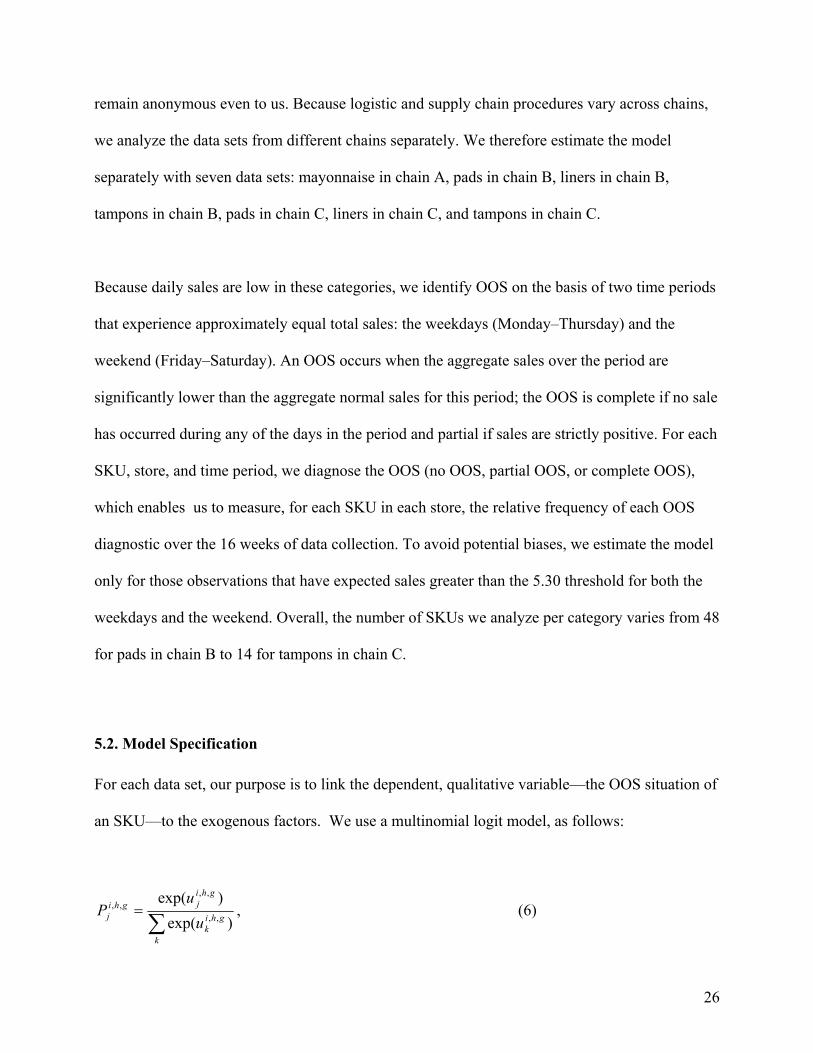
5.2. Model Specification
For each data set, our purpose is to link the dependent, qualitative variable—the OOS situation of
an SKU—to the exogenous factors. We use a multinomial logit model, as follows:
∑=
k
ghik
ghijghi
j uu
P)exp(
)exp(,,
,,,, , (6)
26
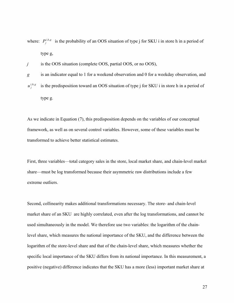
where: is the probability of an OOS situation of type j for SKU i in store h in a period of
type g,
ghijP ,,
j is the OOS situation (complete OOS, partial OOS, or no OOS),
g is an indicator equal to 1 for a weekend observation and 0 for a weekday observation, and
ghiju ,, is the predisposition toward an OOS situation of type j for SKU i in store h in a period of
type g.
As we indicate in Equation (7), this predisposition depends on the variables of our conceptual
framework, as well as on several control variables. However, some of these variables must be
transformed to achieve better statistical estimates.
First, three variables—total category sales in the store, local market share, and chain-level market
share—must be log transformed because their asymmetric raw distributions include a few
extreme outliers.
Second, collinearity makes additional transformations necessary. The store- and chain-level
market share of an SKU are highly correlated, even after the log transformations, and cannot be
used simultaneously in the model. We therefore use two variables: the logarithm of the chain-
level share, which measures the national importance of the SKU, and the difference between the
logarithm of the store-level share and that of the chain-level share, which measures whether the
specific local importance of the SKU differs from its national importance. In this measurement, a
positive (negative) difference indicates that the SKU has a more (less) important market share at
27

the store than at the chain level. As we expected, these two variables are not correlated. Another
problem results from the correlation among store surface, the number of references in the
category, and the total sales in the category. We include category sales (in log form) in the
equation rather than store surface, because we believe it is a better indicator of the economic
stakes associated with the product category in the store. For the number of references, because we
wish to measure the assortment policy of the store, given the constraints of its size, we regress
the observed number of references on store surface (using a nonlinear regression with a classical
exponential form) and use the residual in Equation (7). This residual equals the difference
between the number of references actually carried by the store in the category and the expected
number of references for a store of that size. In this manner, we measure the assortment policy of
the store. If the residual is positive (negative), the store follows a large (reduced) assortment
policy compared with a typical store of the same size.
Third, we introduce additional control variables beyond those in our conceptual framework on
the basis of discussions with retailing executives and store managers. These discussions
identified three important factors that cannot be generalized across categories: (1) Different
manufacturers typically are organized differently in terms of logistics. Therefore, we expect
different performances in terms of OOS, though it seems impossible to draw conclusions across
categories because the manufacturers are not the same in different categories; (2) Many product
categories offer a variety of packaging types (e.g., jars versus tubes) and sizes (e.g., family
packages versus individual portions) that may differ in terms of logistical complexity. Again, we
expect different performances in terms of OOS and recognize the difficulty of drawing
conclusions across categories that vary in terms of the types and sizes of packages; and (3) Some
categories offer different varieties of the product, such as plain versus light mayonnaise, which
28

may create similar problems. Overall, because manufacturers, varieties, sizes, and packages differ
across categories, it is impossible to develop either a unified conceptual framework about them or
generalizable hypotheses. However, we include in each category a set of indicator variables to
avoid specification errors. Furthermore, this set is complex because the factors are not orthogonal
in the data. Typically, different manufacturers offer different varieties in different sizes and
packaging forms. Each indicator variable therefore corresponds to one specific combination that
is actually observed in the category (e.g., a small jar of plain mayonnaise offered by brand B).
Finally, the time period indicator variable g (weekdays versus weekend) is self-explanatory, and
no indicator variable is necessary for seasonality. Pads, tampons, and liners are intrinsically
nonseasonal, and the 16-week observation period showed no seasonality for mayonnaise.
Therefore, the equation for the predisposition is as follows: ghiju ,,
( ) gDMSChainMSCatSalesu jk
ikkj
hij
ijj
hjj
ghij θληδγβα ++∆++∆++= ∑,h,, lnlnfRe , (7)
where j, i, h, and g are indices of the OOS situation, SKU, store, and time period,
respectively;
hCatSales is the logarithm of the total category sales (over 16 weeks) in store h, so that
CatSales where
= ∑
∈ hIi
hih Sales ,ln hI is the set of all the SKUs carried in store h;
hRef∆ is the difference between the number of references carried by store h in the category and
the expected number of references, given store h’s size;
( )iChainMSln is the logarithm of the chain-level market share of SKU i, which is equal to
the total sales of SKU i across the sample of stores during the 16
29

weeks divided by the total sales of all SKUs across the sample of stores during
the 16 weeks;
is the difference between the logarithm of the market share of SKU i
in store h and the logarithm of its chain-level market shareChainMS , given by
hiMS ,ln∆ hiMS ,
i
( ) ( )ihihi ChainMSMSMS lnlnln ,, −=∆ ; and,
ikD is the indicator describing whether SKU i corresponds to the specific combination k (a
specific variety offered by a specific manufacturer in a specific size and
package1).
6. Results
6.1. Frequency of OOS Occurrences
In Table 1, we present the OOS frequencies observed for each data set. The conclusions are very
homogeneous: Complete OOS are much less frequent than partial OOS, regardless of the product
category and retail chain. The incidence of complete OOS varies between 0.6% and 3.5%, much
less than the incidence of partial OOS, which varies between 9.4% and 15.6%. In many OOS
cases, only a fraction of the expected sales are lost, because the SKU is available during at least
part of the time period. In Table 1, we also show that for pads, liners, and tampons, chain C has
fewer partial and complete OOS than chain B. In more general terms, OOS performances are
1 As we explained previously, these indicator variables describe the actual observed combinations among manufacturers (three manufacturers and one private label for mayonnaise; four manufacturers and one private label for each pads data set; four manufacturers and one private label for each liners data set; two manufacturers and one private label for tampons in chain B; and two manufacturers for tampons in chain C), varieties (light, flavored, and plain for mayonnaise; thick winged, thick non-winged, ultra-thin winged, and ultra-thin non-winged for pads; normal, string, or micro for liners; and cardboard mini or mixed, digital mini or mixed, plastic mixed, cardboard normal, digital normal, plastic normal, cardboard super or super plus, digital super or super plus, and plastic super or
30

likely to differ markedly between chains because of the differences in their supply chain
organization and assortment policies.
Table 1 Average OOS Rates by Category and Chain
Mayonnaise
Pads Liners Tampons
Chain A Chain B Chain C Chain B Chain C Chain B Chain C
Number of SKUs
41 24 18 48 37 24 14
Number of Observations
84,076 28,710 23,422 63,963 50,757 28,825 15,056
Complete OOS Frequency
1.1% 3.5% 0.8% 1.3% 0.6% 2.7% 1.6%
Partial OOS Frequency
10.4% 15.6% 10.5% 14.6% 9.4% 13.8% 11.8%
No OOS Frequency
88.5% 80.9% 88.7% 84.1% 89.9% 83.5% 86.6%
6.2. Determinants of OOS
In Tables 2 and 3, we present the results of our multinomial logit regression, which supports
seven of our ten hypotheses. Likelihood ratio tests, as we report in Table 2, confirm that all the
variables we study have a significant impact on explaining both partial and complete OOS
occurrences. Store sales in the category and SKU store market share are the most significant
variables for all items except pads in chain B. In contrast, the number of references in the
category represents the least significant variable for all data sets.
super plus for tampons), and package size (large jar, medium jar, small jar, tube, and plastic bottle for mayonnaise; nothing for the other categories).
31

Table 2 Likelihood Ratio Tests
Mayonnaise
Chain A
Pads
Chain B
Pads
Chain C
Liners
Chain B
Liners
Chain C
Tampons
Chain B
Tampons
Chain C
Store Sales in the
Category
1236.4 788.0 316.7 398.3 199.5 402.7 270.4
Number of
References
201.5 95.6 62.1 3.5 ns 11.1 30.8 42.4
SKU’s Chain
Market Share
239.0 1124.8 125.8 157.3 18.2 65.0 15.1
SKU’s Local
Market Share
561.6 1716.9 305.2 504.4 27.2 999.9 154.5
Notes: The chi-square value for 1 degree of freedom with a probability of 0.001 equals 10.83.
32

Table 3 Estimated Coefficients for the Multinomial Logit Regressions
Mayonnaise Pads Liners Tampons
Chain A Chain B Chain C Chain B Chain C Chain B Chain C
Complete OOS
Store Sales in the Category
-0.77a (187.9)
0.11a (9.1)
-0.95a (91.6)
-0.44a (25.9)
-1.30a (109.3)
-0.35a (34.5)
-0.79a (46.3)
SKU’s Chain Market Share
-0.98a (136.5)
-1.21a (1043.1)
-0.90a (53.6)
-0.83a (97.9)
-0.68a (12.5)
-0.38a (13.6)
-1.29c (4.2)
SKU’s Local Market Share
-0.78a (110.3)
-1.92a (1584.6)
-2.49a (229.9)
-2.80a (516.1)
-0.76a (13.1)
-2.92a (862.5)
-2.49a (128.2)
Number of References
-.09a (115.5)
0.11a (85.8)
-0.03c (2.9)
-0.02 (0.26)
-0.06 (1.2)
-0.10a (27.8)
-0.30a (30.2)
Private Label Indicator
Variables*
4- a 1 ns
4- a 2- a
1- c 2 ns 1- a 5- a No
private label
Partial OOS
Store Sales in the Category
0.56a (1042.3)
0.47a (785.6)
0.39a (219.5)
0.48a (359.3)
0.35a (94.0)
0.50a (347.6)
0.67a (218.5)
SKU’s Chain Market Share
0.33a (440.2)
0.13a (44.9)
0.36a (74.3)
0.24a (66.9)
0.17a (7.2)
0.40a (45.1)
0.78a (10.3)
SKU’s Local Market Share
0.54a (105.8)
0.21a (49.8)
0.48a (79.5)
0.23a (21.9)
0.24a (14.0)
0.44a (58.0)
0.64a (31.1)
Number of References
-0.03a (107.5)
0.02a (14.7)
-0.04a (61.5)
0.02c (3.1)
-0.05a (10.2)
-0.02c (4.6)
-0.12a (21.1)
Private Label Indicator
Variables*
4+ a 1 ns
3- a 1- b
3 ns 1+ a 1 ns
1+ a 2- a 1- c 2 ns
No Private label
Chi square 2542.3 8340.3 1112.4 1409.7 382.4 3184.9 557.7
df 58 42 36 28 20 42 30 ap < 0.001 bp < 0.01 cp < 0.05. *We report only the sign and significance of the coefficients of the indicator variables that
33

account for the combination of the private label nature of the product, its variety type, and package size for simplicity.
In support of H1, we find that in stores with high category sales, there are fewer complete OOS
(six data sets) and more partial OOS (all seven data sets). The results are significant, with the
exception of the coefficient relative to complete OOS for pads in chain B, which is slightly
significant and has the wrong sign, a result for which we have no post hoc explanation. Stores
with higher sales in the category represent higher economic stakes for retailers and enjoy better
forecasting, ordering, and delivering processes. Both these factors may reduce the frequency of
complete OOS. At the same time, these stores have higher sales rotations, which require more
frequent replenishments, create tighter logistics constraints, and may cause the increased
frequency of partial OOS.
As we predicted, complete OOS are less likely and partial OOS more likely for SKUs with higher
market shares for both chain-level market shares (H2) and store-level market shares (H3). The
results are significant and completely homogeneous across data sets, with 14 negative
coefficients for complete OOS and 14 positive coefficients for partial OOS. As we discussed
previously, the lower frequency of complete OOS for items with higher market shares may be
explained by higher economic stakes and easier forecasting and ordering processes. In addition,
the higher frequency of partial OOS can be attributed to higher rotations, which create problems
with regard to the allocation of shelf space and demand frequent replenishments.
Although our previous hypotheses are confirmed by our empirical analysis, we do not find
support for our hypotheses related to the number of references. We expected more complete and
more partial OOS in stores that carry more references in a category (H4), but we find mixed
34
results, with a majority of them in contrast to our expectations. Stores with more references tend
to have fewer complete OOS (six data sets) and fewer partial OOS (five data sets). If we set aside
those coefficients that are not significant at the 1% level, seven of the nine significant coefficients
are negative. Thus, we find that carrying more references than a typical store of the same size
tends to decrease the occurrence of OOS. Our main interpretation of these unexpected results
relies on the argument provided by some of the managers we interviewed. If a store decides to
offer a larger assortment than other stores of a similar size, it also should engage sufficient
logistical resources to guarantee the availability of that assortment; otherwise , the policy of large
assortment could backfire. In addition, a store with a large assortment is less likely to experience
“cascade” OOS, in which an OOS for one item leads consumers to purchase another item, which
then becomes an OOS, and so forth. In contrast, cascade OOS should be more likely in stores
with reduced assortments.
For private labels, we expected fewer complete OOS (H5a) and more partial OOS (H5b). The
results here must be interpreted with care, because SKUs sold as private labels do not cover all
product varieties, nor all package–size combinations. For example, private labels may be
available only for plain varieties (rather than special flavors) and in large package sizes (rather
than individual portions). The SKUs sold as private labels therefore are not identical to those sold
as national brands, and we can only examine the coefficients of the indicator variables for those
brand–variety–package size combinations that are sold as private labels. The results are
contradictory. For complete OOS, in support of H5a, 17 of the 20 coefficients related to the
private label indicator variables are negative and significant (the remaining 3 are not significant),
which suggests that complete OOS are less frequent for private labels. However, for partial
OOS, H5b is supported for mayonnaise and liners (4 of 5 coefficients for the former and 2 of 3
35

for the latter are significantly positive; the remainder are not significant) but not for pads or
tampons in chain B, and we find no significant result for pads and tampons in chain C. It
therefore would be hazardous to attempt to draw general conclusions from these findings.
The great majority of the other indicator variables that refer to specific combinations of
manufacturer identity, product variety, and package size generate significant likelihood ratio
tests. This finding confirms our expectations that these variables have an affect on OOS
occurrences. However, as we have discussed, the complex brand–variety–package size
combinations differ across categories, which makes it difficult to interpret their estimated
coefficients.
Finally, the indicator variable for the type of time period (weekdays versus weekend) generates a
significant likelihood ratio. Complete OOS are more likely during a weekend period than during
a weekdays period, whereas partial OOS are less likely. This result is due to the length of the
periods. Mechanically, the observation of no sales on four successive days (Monday–Thursday)
is less likely than over two days (Friday and Saturday). In contrast, the observation of a partial
OOS is more likely during a four day period than a two day period.
7. Conclusions, Limitations, and Further Research
7.1 Main Conclusions
To our knowledge, this is the first academic research on the frequency and causes of OOS that is
based on store-level scanner data. Most previous research relies on interviews (Campo et al.
36
2000, Emmelhainz et al. 1991, Zinn and Liu 2001) or experiments (Bell and Fitzsimons 1999,
Charlton and Ehrenberg 1976, Fitzsimons 2000), and managerial analyses often are based on
store audits. The use of household scanner panel data is more recent; however, Bell and
Fitzsimons (1999) and Campo and colleagues (2003) both focus on consumer reactions to OOS
in a few stores rather than on the frequency and causes of OOS in many stores.
Our first contribution is to introduce a new measure of OOS computed with IRI scanner data (IRI
France 2002). In contrast with store audits, this measure is based on readily available, reliable,
accurate scanner data recorded at the detailed store/SKU/period level. Rather than relying on a
dichotomous, instantaneous, and myopic definition of OOS, as store audits provide, our measure
derives from a continuous, integrative conceptual definition that is based on the sales lost due to
OOS by each SKU in each store during each period of interest. This synthetic measure combines
into a single number the impact of the frequency, duration, and importance of all OOS incidents
during a specified period. Defined by a precise algorithm, it can be applied easily on a very large
scale to thousands of items and hundreds of stores. As such, it can become the basis of an
automatic OOS diagnosis tool that both retailers and manufacturers can use to detect good and
bad stores and SKUs in term of OOS. It also can be applied easily in different countries.
Our second contribution is to introduce a major conceptual distinction between complete OOS
and partial OOS that improves our understanding of the mechanisms underlying OOS
occurrences. For each of our seven data sets, complete OOS are much less frequent than are
partial OOS, which indicates that retailers and manufacturers try to avoid complete OOS because
they imply a complete loss of sales. It also shows the recent success obtained by effective
manufacturer–retailer collaboration in the supply chain. Through the growing diversity of
37
procedures included in efficient consumer response (ECR) programs, such as computer-assisted
ordering (CAO) and continuous replenishment programs (CRP), major improvements have been
achieved in the supply chain. At the same time, the relatively high frequency of partial OOS
underlines the necessity for retailers to continue to improve their replenishment procedures.
Our third contribution is our analysis of the causes of OOS. Our results are homogeneous across
product categories and support the main hypotheses of our conceptual framework. In addition,
they strongly justify our conceptual distinction between complete and partial OOS, in that they
confirm that explanatory variables generally have opposite effects on these two types of OOS. As
retailers try to limit OOS consequences to a partial OOS and avoid a complete OOS, they give
priority to those cases that represent higher economic stakes. With these findings, we show that
complete OOS are less frequent in larger stores with high category sales, for SKUs with higher
market shares (at both local and chain levels), and for private labels. In line with our hypothesis
that the two forms of OOS react differently to the explanatory variables and because of the
logistical difficulties created by higher sales rotations, partial OOS are more frequent in larger
stores and for SKUs with higher market shares (at both local and chain levels). In addition, there
are clear variations across retailing chains in terms of OOS rates. We also observe significant
differences among manufacturers, which may be due to differences in their logistical organization
and economic power, between types of packages and product varieties. However, these
differences are impossible to generalize across product categories. Finally, we observe one major
unexpected result, namely, both complete and partial OOS are less frequent when the assortment
size is greater, possibly because stores that choose a large assortment policy are likely to support
it with appropriately increased logistic support.
38

7.2 More on Partial OOS
The relatively high frequency of partial OOS calls for additional managerial questions: What
percentage of expected sales is lost during a partial OOS? What is the relative influence of partial
versus complete OOS on sales losses due to OOS? Are partial OOS more damaging than
complete OOS? A partial OOS could represent only a few lost sales—say, 10% of the expected
sales if the store replenishes the shelf very efficiently—or a loss of most sales—such as 90%
because of inefficient replenishment. The economic consequences would be very different in
these two cases. In Figure 3, we display the results observed in our seven data sets by plotting
the empirical distribution of the percentage of lost sales across all observed occurrences of partial
OOS.
Figure 3 Distribution of the Percentage of Lost Sales Due to Partial OOS
100,090,080,070,060,050,040,030,020,010,0
Pads - Chain C1200
1000
800
600
400
200
0
9080706050403020100
Pads - Chain B1600
1400
1200
1000
800
600
400
200
09080706050403020100
Liners - Chain B4000
3000
2000
1000
0
100,090,080,070,060,050,040,030,020,010,0
Liners - Chain C3000
2000
1000
0
90,080,070,060,050,040,030,020,010,0
Tampons - Chain B1600
1400
1200
1000
800
600
400
200
0
90,080,070,060,050,040,030,020,0
Tampons - Chain C1000
800
600
400
200
0
100,090,080,070,060,050,040,030,020,010,00,0
Mayonnaise - Chain A1600
1400
1200
1000
800
600
400
200
0
Despite small differences, the distributions are strikingly similar across categories: They are
unimodal and roughly symmetrical, and the mode (and mean) correspond to lost sales that are
39

close to 50% of the expected sales. Even if we observe a few extreme values, the dispersion
around the mean is moderate, with standard deviations of approximately 10%–15%.
With these results, we can estimate the economic consequences of partial OOS and compare them
with the economic consequences of complete OOS (Table 4). For example, for liners in chain B,
the frequency of complete OOS is 1.3%, which, by definition, leads to lost sales equal to 1.3% of
expected sales.
Table 4 Estimation of Lost Sales Induced by Complete and Partial OOS
Mayonnaise Pads Liners Tampons
Chain A Chain B Chain C Chain B Chain C Chain
B
Chain C
Complete OOS
Frequency (a)
1.1% 3.5% 0.8% 1.3% 0.6% 2.7% 1.6%
Partial OOS
Frequency (b)
10.1% 15.3% 10.2% 14.3% 9.3% 13.5% 11.5%
Average Percentage
of Lost Sales (c)
50.6% 43.5% 53.8% 45.4% 53.6% 47.3% 55.0%
Standard Deviation 12.4 14.0 11.7 14.1 12.2 12.7 11.4
Average Loss Due to
Partial OOS (d)*
5.1% 6.7% 5.5% 6.5% 5.0% 6.4% 6.3%
Total Loss (e)** 6.6% 10.2% 6.3% 7.8% 5.6% 9.1% 7.9%
Share of Lost Sales
Due to Complete
OOS (f)***
16.7% 34.3% 12.7% 16.7% 10.7% 29.7% 20.3%
*(d) = (b) × (c). **(e) = (a) + (d). ***(f) = (a)/(e). The frequency of partial OOS is 14.3%, which generates average sales losses equal to 45.4% of
the expected sales. By combining the two numbers, we estimate that partial OOS lead to sales
40

losses equal to 6.5% (14.3% times 45.4%) of the expected sales. Therefore, the overall impact of
OOS for liners in chain B is a loss of sales equal to 7.8% (1.3% plus 6.5%) of the expected sales.
Note that this percentage is roughly half the aggregate frequency of OOS (1.3% plus 14.3%, or
15.6%).
To find the relative weight of complete OOS in the total sales losses due to OOS for liners in
chain B, we find that it is equal to 1.3% divided by 7.8%, or 16.7%, a rather low figure. As we
show in Table 4, this share of lost sales due to complete OOS remains below 50% for all seven
data sets, varying between 10.7% and 34.3%. Regardless of the category and chain, partial OOS
induce more sales losses than do complete OOS, which should be regarded as a positive result by
retailers. However, it also should encourage them to implement even more efficient logistic
processes to improve replenishment procedures and further reduce the impact of partial OOS.
However, as stated by a senior marketing vice president of a leading chain in one of our
interviews, “Replenishment dysfunctions could of course be easily improved with additional staff
but at which extra cost? We are better off with some OOS than with additional personnel costs
which are so heavy in our country.” For manufacturers, this large proportion of lost sales
associated with partial OOS poses a challenge, because they cannot intervene in in-store
replenishment procedures.
As evidenced by Figure 3, there are variations in the percentage of lost sales around the modal
value of 50%, which indicates that we must analyze the causes of these variations further. Which
items, among those suffering a partial OOS, lose more sales, and which lose fewer sales? We ran
ordinary least square regressions on each data set, using the percentage of lost sales as the
dependent variable. (We use the percentage of lost sales, rather than the absolute level of lost
41

sales, to ensure comparability across stores and SKUs.) For the explanatory variables, we believe
that, if the importance of a particular SKU leads the retailer to try to avoid a complete OOS, the
retailer also will attempt to limit the magnitude of the sales losses associated with a partial OOS.
We therefore hypothesize that, if a factor leads to a decrease (increase) in the likelihood of a
complete OOS for an SKU, it also will lead to a decrease (increase) in the magnitude of a partial
OOS for that same SKU. We use the same set of explanatory variables as those in our main
multinomial logit regression (Equation 7) and report the results for each of the seven data sets in
Table 5 (for brevity, we omit the coefficients relative to variables that cannot be generalized
across product categories, such as those relative to manufacturers, product varieties, and package
types and sizes, though these variables were included in the regressions). Most of the explanatory
variables that were significant in our main analysis remain significant with the predicted sign, in
support of our hypothesis that factors that reduce the frequency of a complete OOS also reduce
the magnitude of a partial OOS. In concrete terms, when there is a partial OOS, it tends to have
smaller consequences in terms of the percentage of lost sales in larger stores and for those items
with higher market shares. However, our results relative to the number of references offered by
the store vary across categories and therefore are difficult to interpret.
42

Table 5 Regressions Explaining the Percentage of Lost Sales in Partial OOS
Mayonnaise Pads Liners Tampons
Chain A Chain B Chain C Chain B Chain C Chain B Chain C
Store Sales in the Category
-15.0 a -14.0 a -14.4 a -12.2 a -17.4 a -13.9 a -14.4 a
Number of References
-.03 0.11 0.09 1.5 0.08 c -0.14 c 0.38 c
SKU’s Chain Market Share
-12.93 a -9.3 a -8.7 a -12.3 a -15.2 a -15.0 a -13.0 a
SKU’s Local Market Share
-14.67 a -14.7 a -10.8 a -13.8 a -17.6 a -13.7 a -10.4 a
Adjusted R² 39.7% 46.3% 35.4% 43.1% 42.1% 46.6% 33.9% ap < 0.001 cp < 0.05.
7.3 Limitations and Further Research
As we have noted, three important restrictions of this research must be kept in mind. First, our
measure of OOS cannot be applied to detect OOS for the slowest moving items because their
sales may equal 0 in a given period despite their availability on the shelf. We therefore have
voluntarily disregarded observations of SKUs with expected sales of less than 5.3 units. Second,
our measure cannot be computed on the basis of individual days for slow moving product
categories because expected sales may be very low for most items, which would lead the measure
to retain too few items. In such cases, the OOS should be analyzed on the basis of two time
periods per week. Third, this measure is not appropriate to detect OOS for promoted items
because both their expected and observed sales typically are far higher than their normal sales.
In addition, we have no specific treatment for seasonality. Although this limitation is not a
problem for our data set, further research in other categories might compute medians for periods
of similar seasonality.
43

Our approach offers an automated approach to the detection of OOS that is applicable to very
large samples, or censuses, of stores and SKUs on the sole basis of store-level sales. It therefore
can be applied in the absence of data about variables that would be difficult to obtain, such as a
promotion by a competitor, the introduction of a new product, and so forth.
Additional research might try to analyze more precisely the impact of the organizational features
of the supply chain between the manufacturer and the retailing chain, within the chain, and within
each store. For the latter, for example, researchers could use measures of storage room and
personnel availability, as well as indicators that describe the shelving and replenishment
procedures.
Finally, it would be of great interest to study the impact of a major but confidential factor,
namely, the global margins associated with each SKU and with the set of SKUs from a specified
manufacturer.
44

References
Abel, A. 1985. Inventories, stock-outs, and production smoothing. Review of Economic Studies
52 283-293.
Ailawadi, K.L., B. Harlam. 2004. An empirical analysis of the determinants of retail margins:
The role of store-brand share. Journal of Marketing 68 147-65.
Anupindi, R., M. Dada, S. Gupta. 1998. Estimation of consumer demand with stock-out based
substitution: An application to vending machine products. Marketing Science 17 406-423.
Balachander, S., P.H. Farquhar. 1994. Gaining more by stocking less: A competitive analysis of
product availability. Marketing Science 13 3-22.
Bawa, K., J.T. Landwehr, A. Krishna. 1989. Consumer response to retailer’s marketing environments: An analysis of coffee purchase data. Journal of Retailing 65 471-494.
Bell, D.R., G.J. Fitzsimons. 1999. An experimental and empirical analysis of consumer response
to stockouts. Working Paper, Marketing Department, The Wharton School, University of
Pennsylvania.
Campo, K., E. Gijsbrechts, P. Nisol. 2000. Towards understanding consumer response to stock-
outs. Journal of Retailing 76 219-42.
Campo, K., E. Gijsbrechts, P. Nisol. 2003. The impact of retailer stockouts on whether, how
much, and what to buy. International Journal of Research in Marketing 20 273-286.
Charlton, P., A.S.C. Ehrenberg. 1976. An experiment in brand choice. Journal of Marketing
Research 13 152-60.
Corstjens, J., M. Corstjens. 1995. Store Wars: The Battle for Mindspace and Shelfspace. New
York: John Wiley & Sons.
45

Corstjens, M., R. Lal. 2000. Building store loyalty through store brands. Journal of Marketing
Research 37 281-291.
Diaz, A. 1996. How many units will be short when stockout occurs? International Journal of
Operations and Production Management 16(4) 112-118.
Drèze, X., S.J. Hoch, M.E. Purk. 1994. Shelf management and space elasticity. Journal of
Retailing 70 301-326.
Emmelhainz, L.W., M.A. Emmelhainz. 1991. Logistics implications of retail stock-outs. Journal
of Business Logistics 12(2) 129-143.
Emmelhainz, M.A., L.W. Emmelhainz, R.J. Stock. 1991. Consumer responses to retail stock-
outs. Journal of Retailing 67 138-147.
Fitzsimons, G.J. 2000. Consumer response to stockouts. Journal of Consumer Research 27 249-
266.
Frechette, D.L. 1999. Stock-outs and supply response estimation under rational expectations.
European Review of Agricultural Economics 26 59-77.
Gerstner, E., J.D. Hess. 1990. Can bait and switch benefit consumers? Marketing Science 9(2)
114-124.
Gruen, T.W., D.S. Corsten, B. Bharadwaj. 2002. Retail Out-of-Stocks: A Worldwide Examination
of Extent, Causes and Consumer Responses. Washington, DC: The Grocery Manufacturers of
America.
Hess, J.D., E. Gerstner. 1987. Loss leader pricing and rain check policy. Marketing Science 6
358-374.
46

IRI France. (2002). Manuel de meilleures pratiques pour la réduction des ruptures en
linéaire. Tome 1, Avril 2002. Paris: IRI-ECR.
Lau, H., A.H. Lau. 1996. Estimating the demand distributions of single-period items having
frequent stockouts. European Journal of Operational Research 92 254-265.
Levy, M., B.A. Weitz. 2001. Retailing Management, 4th ed. New York: McGraw-Hill.
Peckham, J. 1963. The consumer speaks. Journal of Marketing 27(4) 21-26.
Schary, P.B., M. Christopher. 1979. The anatomy of a stock-out. Journal of Retailing 55(2) 59-
70.
Uncles, M.D., A.S.C. Ehrenberg, K. Hammond. 1995. Patterns of buyer behavior: Regularities,
models and extensions. Marketing Science 14(3, 2 of 2) G71-G78.
Van Delft, Ch., J.P. Vial. 1996. Discounted costs, obsolescence and planned stockouts with the
EOQ formula. International Journal of Production Economics 44 255-265.
Walter, C., J. Grabner. 1975. Stockout cost models: Empirical tests in a retail situation. Journal
of Marketing 39(3) 56-68.
Wilkie, W.L., C.F. Mela, G.T. Gundlach. 1998. Does “bait and switch” really benefit consumers?
Marketing Science 17 273-282.
Zinn, W., P.C. Liu. 2001. Consumer response to retail stock-outs. Journal of Business Logistics
22 49-72.
Zinszer, P.H., J.A. Lesser. 1981. An empirical evaluation of the role of stock-out on shopper
patronage processes. Advances in Consumer Research 8 221-224.
47