Earth Syst. Dynam., 9, 701–715, 2018https://doi.org/10.5194/esd-9-701-2018© Author(s) 2018. This work is distributed underthe Creative Commons Attribution 4.0 License.

Assessing the impact of a future volcanic eruption ondecadal predictions

Sebastian Illing1, Christopher Kadow1, Holger Pohlmann2, and Claudia Timmreck2

1Freie Universität Berlin, Institute of Meteorology, Berlin, Germany2Max Planck Institute for Meteorology, Hamburg, Germany

Correspondence: Sebastian Illing (sebastian.illing@met.fu-berlin.de)

Received: 22 January 2018 – Discussion started: 2 February 2018Accepted: 27 April 2018 – Published: 6 June 2018

Abstract. The likelihood of a large volcanic eruption in the future provides the largest uncertainty concerningthe evolution of the climate system on the timescale of a few years, but also an excellent opportunity to learnabout the behavior of the climate system, and our models thereof. So the following question emerges: howpredictable is the response of the climate system to future eruptions? By this we mean to what extent will thevolcanic perturbation affect decadal climate predictions and how does the pre-eruption climate state influencethe impact of the volcanic signal on the predictions? To address these questions, we performed decadal forecastswith the MiKlip prediction system, which is based on the MPI-ESM, in the low-resolution configuration for theinitialization years 2012 and 2014, which differ in the Pacific Decadal Oscillation (PDO) and North AtlanticOscillation (NAO) phase. Each forecast contains an artificial Pinatubo-like eruption starting in June of the firstprediction year and consists of 10 ensemble members. For the construction of the aerosol radiative forcing, weused the global aerosol model ECHAM5-HAM in a version adapted for volcanic eruptions. We investigate theresponse of different climate variables, including near-surface air temperature, precipitation, frost days, and seaice area fraction. Our results show that the average global cooling response over 4 years of about 0.2 K and theprecipitation decrease of about 0.025 mm day−1 is relatively robust throughout the different experiments andseemingly independent of the initialization state. However, on a regional scale, we find substantial differencesbetween the initializations. The cooling effect in the North Atlantic and Europe lasts longer and the Arctic seaice increase is stronger in the simulations initialized in 2014. In contrast, the forecast initialized in 2012 witha negative PDO shows a prolonged cooling in the North Pacific basin.

1 Introduction

More and more attention has been paid to decadal climateprediction in the last decade (Meehl et al., 2009; Smith et al.,2007). This research field tries to fill the gap between short-term (weather to seasonal) predictions on the one hand andlong-term climate projections on the other hand. Decadalpredictability comes mainly from the multi-year memory ofthe ocean. The memory in the ocean arises, for instance, fromthe persistence of ocean heat content anomalies and fromproperly initialized ocean dynamics and circulation (e.g.,Guemas et al., 2012; Matei et al., 2012). A detailed explana-tion of the principles behind decadal prediction can be foundin Kirtman et al. (2013).

A number of studies revealed that there is at least poten-tial prediction skill in near-surface air temperature, precipi-tation, and three-dimensional variables like air temperatureor geopotential height (Goddard et al., 2013; Kadow et al.,2016; Stolzenberger et al., 2016). Recently, some institutionslike the UK Met Office and the German project for decadalclimate prediction, MiKlip (Marotzke et al., 2016), havestarted issuing decadal climate forecasts for near-surface airtemperature on a regular – but still experimental – basis(metoffice.gov, 2017; Smith et al., 2013; Vamborg et al.,2017).

The skill of decadal predictions is usually evaluated us-ing hindcast simulations (e.g., Doblas-Reyes et al., 2013;

Published by Copernicus Publications on behalf of the European Geosciences Union.

702 S. Illing et al.: Assessing the impact of a future volcanic eruption on decadal predictions

Kim et al., 2012), and it is assumed that external forcing isknown over the whole simulation period. In a real decadalforecast, this assumption is invalid because rapid forcingchanges like volcanic eruptions cannot be predicted in ad-vance. Hence, strong tropical volcanic eruptions (SVEs) arearguably the largest source of uncertainty for this type of pre-diction. They increase the stratospheric aerosol load, whichleads to a reduction of global mean surface temperature dueto the reduced incoming solar radiation. For instance, afterthe tropical Pinatubo eruption in 1991, a global peak cool-ing of about 0.4 K (Thompson et al., 2009) was observed.Regionally, however, warm anomalies are found after SVEs,e.g., the winter warming over Europe in the first two wintersafter the eruption (Kirchner et al., 1999; Robock and Mao,1992). Apart from temperature, SVEs also have an impacton atmospheric composition, atmosphere and ocean dynam-ics, and the hydrological cycle (e.g., Robock, 2000; Timm-reck, 2012). The major volcanic eruptions that occurred since1850 were followed by a period of reduced global precipita-tion (Robock and Mao, 1992; Gu and Adler, 2011; Iles andHegerl, 2014), and volcanoes can also modulate the African,Asian and South American monsoon systems (e.g., Josephand Zeng, 2011; Iles and Hegerl, 2013; Liu et al., 2016).Sea ice in the Northern Hemisphere is also affected by largevolcanic eruptions that occurred between 1850 and 2005,and SVEs can cause up to a decade of increased Arctic seaice extent (Ding et al., 2014; Gagné et al., 2017). Gagnéet al. (2017), for example, demonstrated that the sea ice re-sponse to SVEs is dependent on pre-eruption temperatureconditions with a warmer pre-eruption climate leading toa stronger sea ice response. There is some evidence from ob-servations and reconstructions that SVEs lead to a positivephase of the Northern Atlantic Oscillation (NAO) in the firstfew winters following the eruption (e.g., Ortega et al., 2015;Swingedouw et al., 2017), but recent model studies suggestthat this signal might not be that robust (Bittner et al., 2016;Ménégoz et al., 2017). It has also been suggested that thepositive NAO response could be better interpreted in terms ofa deficit of negative NAO circulations (Toohey et al., 2014).

There are only a few studies that focus on how vol-canic forcing impacts decadal climate predictions. Meehlet al. (2015) showed in a multi-model study that the Pinatuboeruption led to a reduction of decadal hindcast skill in Pacificsea surface temperatures. Timmreck et al. (2016) demon-strated that neglecting volcanic aerosol in decadal predictionssignificantly affects hindcast skill for near-surface air tem-perature and leads to a skill reduction in most regions up toprediction year 5. Bethke et al. (2017) explored how possi-ble future volcanic eruptions impact climate variability underRCP4.5 and found that the consideration of volcanic forcingenhances climate variability on annual to decadal timescales.However, not every volcanic eruption influences the climatein the same way. Zanchettin et al. (2013) showed in a casestudy of the Tambora eruption in 1815 that near-surfaceatmospheric and oceanic dynamics are significantly influ-

enced by climate background conditions. Furthermore, hind-casts with the atmosphere-only HADGEM1 model (Marshallet al., 2009) showed that the climate anomalies in the firstpost-volcanic winter over Europe are strongly dependent onthe stratospheric conditions in early winter.

Historically explosive tropical volcanic eruptions havea statistical recurrence frequency of about 50 to 100 years(Ammann and Naveau, 2003; Self et al., 2006). With thePinatubo eruption almost 27 years ago and the recent ongo-ing unrest of Mount Agung in Indonesia, the following ques-tion arises: what would happen if a large volcanic eruptionoccurred in the present and how dependent would the resultsbe on the start year and the associated initial climate state?In this paper, we investigate the response of different climatevariables, including near-surface air temperature (TAS), pre-cipitation (PR), number of frost days (FD), and sea ice areafraction (SIC), to an artificial Pinatubo-like eruption happen-ing in June of the first simulation year for two initializationsthat differ in their initial state. To quantify the volcanic ef-fect we compare our multi-year forecasts with the simula-tions without a volcanic eruption performed with the MiKlipprediction system (Pohlmann et al., 2013).

In Sect. 2 we describe the models used and our experimen-tal setup, while the results of our analysis for different vari-ables are presented in Sect. 3. In Sect. 4 we draw conclusionsand discuss our results.

2 Model description and experimental setup

2.1 Model description

We perform our forecasts containing a Pinatubo-like erup-tion with the baseline1 version of the MiKlip prediction sys-tem (Marotzke et al., 2016; Pohlmann et al., 2013), whichis based on the coupled Max Planck Institute–Earth SystemModel (MPI-ESM; Giorgetta et al., 2013; Jungclaus et al.,2013). The MPI-ESM is an Earth system model with atmo-sphere, ocean, and dynamic vegetation components. We usethe “low-resolution” (LR) configuration of the baseline1 sys-tem, which has a resolution of T63 with 47 vertical levels inthe atmosphere and an oceanic resolution of 1.5◦ with 40 ver-tical levels. The atmospheric component ECHAM6 (Stevenset al., 2013) is initialized with full fields of temperature, vor-ticity, divergence, and sea level pressure from the ECMWFatmosphere reanalysis (Dee et al., 2011). The oceanic com-ponent MPI-OM (Jungclaus et al., 2013) is initialized usinganomaly fields from the ECMWF ocean reanalysis system 4(Balmaseda et al., 2013) including temperature and salinity.For decadal forecasting, an operational model system for therapid model-based assessment of the decadal-scale climateimpact is needed in the case of any major volcanic erup-tion. However, any modification to the climate model itselfrequires a retuning (Mauritsen et al., 2012), a new controlrun with constant forcing to make sure the model simulatesa stable climate, and a new ensemble of historical runs as

Earth Syst. Dynam., 9, 701–715, 2018 www.earth-syst-dynam.net/9/701/2018/

S. Illing et al.: Assessing the impact of a future volcanic eruption on decadal predictions 703

Year 1 Year 2 Year 3Simulation time

80

60

40

20

0

20

40

60

80

Latit

ude

Erup

tion

in J

une

(a) Simulated AOD

0.0

0.1

0.2

0.3

0.4

0.5

2012 2013 2014 2015Time

40

20

0

20

40

(c) PDO

2012 2013 2014 2015Time

20 000

10 000

0

10 000

20 000

(b) NAO

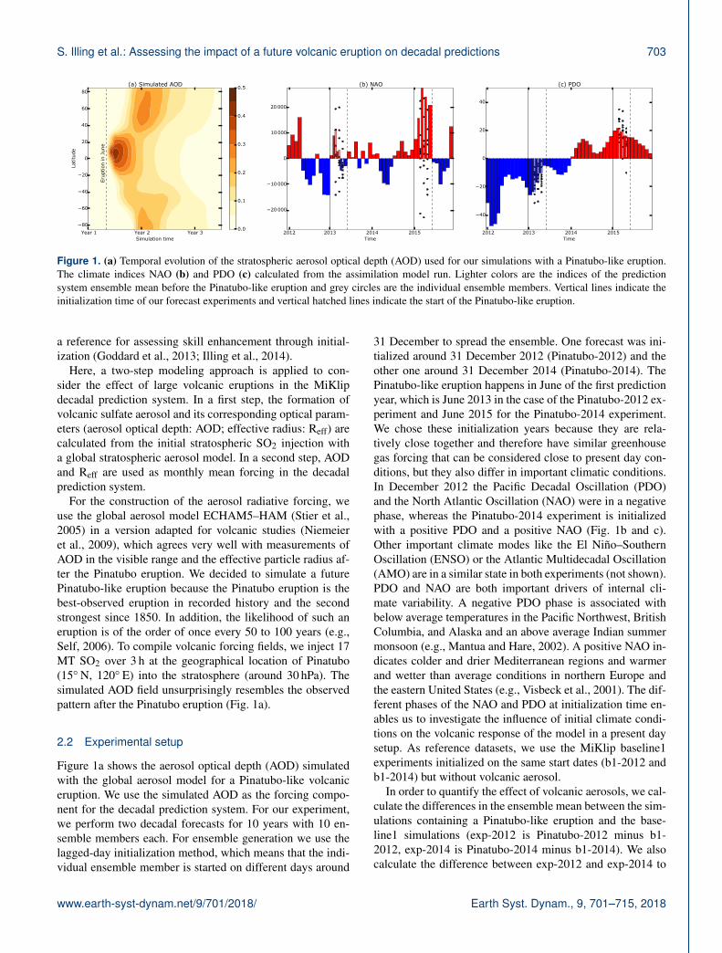
Figure 1. (a) Temporal evolution of the stratospheric aerosol optical depth (AOD) used for our simulations with a Pinatubo-like eruption.The climate indices NAO (b) and PDO (c) calculated from the assimilation model run. Lighter colors are the indices of the predictionsystem ensemble mean before the Pinatubo-like eruption and grey circles are the individual ensemble members. Vertical lines indicate theinitialization time of our forecast experiments and vertical hatched lines indicate the start of the Pinatubo-like eruption.

a reference for assessing skill enhancement through initial-ization (Goddard et al., 2013; Illing et al., 2014).

Here, a two-step modeling approach is applied to con-sider the effect of large volcanic eruptions in the MiKlipdecadal prediction system. In a first step, the formation ofvolcanic sulfate aerosol and its corresponding optical param-eters (aerosol optical depth: AOD; effective radius: Reff) arecalculated from the initial stratospheric SO2 injection witha global stratospheric aerosol model. In a second step, AODand Reff are used as monthly mean forcing in the decadalprediction system.

For the construction of the aerosol radiative forcing, weuse the global aerosol model ECHAM5–HAM (Stier et al.,2005) in a version adapted for volcanic studies (Niemeieret al., 2009), which agrees very well with measurements ofAOD in the visible range and the effective particle radius af-ter the Pinatubo eruption. We decided to simulate a futurePinatubo-like eruption because the Pinatubo eruption is thebest-observed eruption in recorded history and the secondstrongest since 1850. In addition, the likelihood of such aneruption is of the order of once every 50 to 100 years (e.g.,Self, 2006). To compile volcanic forcing fields, we inject 17MT SO2 over 3 h at the geographical location of Pinatubo(15◦ N, 120◦ E) into the stratosphere (around 30 hPa). Thesimulated AOD field unsurprisingly resembles the observedpattern after the Pinatubo eruption (Fig. 1a).

2.2 Experimental setup

Figure 1a shows the aerosol optical depth (AOD) simulatedwith the global aerosol model for a Pinatubo-like volcaniceruption. We use the simulated AOD as the forcing compo-nent for the decadal prediction system. For our experiment,we perform two decadal forecasts for 10 years with 10 en-semble members each. For ensemble generation we use thelagged-day initialization method, which means that the indi-vidual ensemble member is started on different days around

31 December to spread the ensemble. One forecast was ini-tialized around 31 December 2012 (Pinatubo-2012) and theother one around 31 December 2014 (Pinatubo-2014). ThePinatubo-like eruption happens in June of the first predictionyear, which is June 2013 in the case of the Pinatubo-2012 ex-periment and June 2015 for the Pinatubo-2014 experiment.We chose these initialization years because they are rela-tively close together and therefore have similar greenhousegas forcing that can be considered close to present day con-ditions, but they also differ in important climatic conditions.In December 2012 the Pacific Decadal Oscillation (PDO)and the North Atlantic Oscillation (NAO) were in a negativephase, whereas the Pinatubo-2014 experiment is initializedwith a positive PDO and a positive NAO (Fig. 1b and c).Other important climate modes like the El Niño–SouthernOscillation (ENSO) or the Atlantic Multidecadal Oscillation(AMO) are in a similar state in both experiments (not shown).PDO and NAO are both important drivers of internal cli-mate variability. A negative PDO phase is associated withbelow average temperatures in the Pacific Northwest, BritishColumbia, and Alaska and an above average Indian summermonsoon (e.g., Mantua and Hare, 2002). A positive NAO in-dicates colder and drier Mediterranean regions and warmerand wetter than average conditions in northern Europe andthe eastern United States (e.g., Visbeck et al., 2001). The dif-ferent phases of the NAO and PDO at initialization time en-ables us to investigate the influence of initial climate condi-tions on the volcanic response of the model in a present daysetup. As reference datasets, we use the MiKlip baseline1experiments initialized on the same start dates (b1-2012 andb1-2014) but without volcanic aerosol.

In order to quantify the effect of volcanic aerosols, we cal-culate the differences in the ensemble mean between the sim-ulations containing a Pinatubo-like eruption and the base-line1 simulations (exp-2012 is Pinatubo-2012 minus b1-2012, exp-2014 is Pinatubo-2014 minus b1-2014). We alsocalculate the difference between exp-2012 and exp-2014 to

www.earth-syst-dynam.net/9/701/2018/ Earth Syst. Dynam., 9, 701–715, 2018

704 S. Illing et al.: Assessing the impact of a future volcanic eruption on decadal predictions

1–4 2–5 3–6 4–7 5–8 6–9 7–10Lead times [yr]

287.4

287.6

287.8

288.0

288.2Te

mpe

ratu

re [

K]

(a)

Initialized 2012Global

Baseline1Pinatubo

Lead times [yr]

287.4

287.6

287.8

288.0

288.2

Tem

pera

ture

[K]

(b)

Initialized 2014Global

Lead times [yr]

279.2

279.4

279.6

279.8

280.0

Tem

pera

ture

[K]

(c)

North Atlantic (60–0 W, 50–65 N)◦ ◦

Lead times [yr]

279.2

279.4

279.6

279.8

280.0

Tem

pera

ture

[K]

(d)

North Atlantic (60–0 W, 50–65 N)◦ ◦

Lead times [yr]

284.5

284.7

284.9

285.1

285.3

285.5

Tem

pera

ture

[K]

(e)

Europe (10 W–35 E, 30–75 N)◦ ◦ ◦

Lead times [yr]

284.5

284.7

284.9

285.1

285.3

285.5

Tem

pera

ture

[K]

(f)

Europe (10 W–35 E, 30–75 N)◦ ◦ ◦

Lead times [yr]

287.5

287.7

287.9

288.1

288.3

288.5,

Tem

pera

ture

[K]

(g)

North Pacific basin (130–250 E, 20–60 N)◦ ◦

Lead times [yr]

287.5

287.7

287.9

288.1

288.3

288.5,

Tem

pera

ture

[K]

(h)

North Pacific basin (130–250 E, 20–60 N)◦ ◦ ◦

Baseline1Pinatubo

1–4 2–5 3–6 4–7 5–8 6–9 7–10

1–4 2–5 3–6 4–7 5–8 6–9 7–10 1–4 2–5 3–6 4–7 5–8 6–9 7–10

1–4 2–5 3–6 4–7 5–8 6–9 7–10 1–4 2–5 3–6 4–7 5–8 6–9 7–10

1–4 2–5 3–6 4–7 5–8 6–9 7–10 1–4 2–5 3–6 4–7 5–8 6–9 7–10

Figure 2. Time series of 4-year running mean ensemble forecast of near-surface air temperature (TAS) anomalies. The blue shows valueswithout volcanic eruption, and red with a Pinatubo-like eruption. (a, c, e, g) Experiments initialized in 2012 and (b, d, f, h) those initializedin 2014. (a, b) Global mean, (c, d) North Atlantic (60◦ W–0◦ E, 50–65◦ N), (e, f) Europe (10◦ W–35◦ E, 30–75◦ N), and (g, h) North Pacificbasin (130–250◦ E, 20–60◦ N). Dashed lines indicate significant differences between the values at the 5 % level.

Earth Syst. Dynam., 9, 701–715, 2018 www.earth-syst-dynam.net/9/701/2018/

S. Illing et al.: Assessing the impact of a future volcanic eruption on decadal predictions 705

quantify the impact of the different initial conditions. Statis-tical significance is determined by using a two-sided t test(Wilks, 2011).

3 Results

3.1 Air temperature

Figure 2 shows a forecast for the 4-year running mean near-surface air temperature (TAS) for different regions. The fore-cast is shown like it would be issued by the MiKlip project(Vamborg et al., 2017). In addition, we present it togetherwith our Pinatubo experiments. The Pinatubo-like eruptionleads to a statistically significant decrease at the 95 % levelin global mean temperature of about 0.2 K on average inprediction years 1–4 in both experiments. The temperaturedifference gets smaller in later years, but is significant untilprediction years 7–10 (Fig. 2a and b). Globally, there is noevident difference between the two experiments. The situa-tion is different in the North Atlantic (NA; Fig. 2c and d). Inthe first prediction years, the volcanic aerosol leads to a tem-perature decrease of about 0.3 K in both experiments. How-ever, in the 2012 experiments, the temperature difference de-creases in prediction years 4–7 and completely vanishes fromyears 5–8. This adjustment is mainly because the b1-2012 ex-periment shows a negative trend in later prediction years andthis negative temperature trend is not evident in the Pinatubo-2012 experiment. In contrast, Fig. 2d shows a constant tem-perature difference between b1-2014 and Pinatubo-2014 forthe whole prediction period. For Europe (Fig. 2e and f) bothinitialization dates show a significant surface cooling in thePinatubo experiments in years 1–4 and 2–5, but the cooling ismore pronounced and stays significant longer until years 4–7 in the 2014 model runs. The difference between the twoinitialization dates 2012 and 2014 is strongest in the North-ern Hemispheric spring and fall (not shown). In 2012 thereis no significant temperature decrease in spring and fall visi-ble due to the Pinatubo-like eruption, whereas the Pinatubo-2014 simulation shows significant temperature drops of up to0.4 K on average. In the North Pacific basin (Fig. 2g and h)where the PDO index is calculated, both experiments showa temperature drop induced by the Pinatubo-like eruption inthe first prediction years with the strongest values in predic-tion years 2–5. However, in the 2012 experiment, which isinitialized with a negative PDO, the temperature differencestays nearly constant and significant over the whole predic-tion period, while in Pinatubo-2014 TAS starts recovering inprediction years 3–6.

This disparity is also visible in the global maps in Fig. 3,which shows TAS for prediction years 1–4 and 7–10. Forboth initialization dates, the Pinatubo-like eruption leads tosignificant cooling over most parts of the tropics, NorthAmerica, and the North Atlantic (Fig. 3a and c) for predic-tion years 1–4. Generally, the cooling effect is strongest overthe continents and reaches up to 1 K over North America.

We found the most substantial differences between the ini-tialization dates in Europe, Siberia, and East Asia (Fig. 3e).In Scandinavia the earlier initialized run shows a slightlypositive effect, whereas the latter one shows a strong cool-ing. Thus, the simulations started with the initial condi-tions of 2014 (e.g., positive PDO and NAO) react morestrongly to stratospheric aerosols released by the Pinatubo-like eruption in these regions. In contrast, exp-2012 showsa significantly stronger cooling over Alaska. The negativePDO phase results in a reduced advection, which means lesswarm air being advected from the North Pacific into this re-gion, a transport which is especially important if solar radia-tion is weakened (Wendler, 2012). In later simulation years,the cooling effect is less pronounced in both experiments(Fig. 3b, d, and f). In exp-2012 some parts of the tropics arestill significantly cooler, and in the North Pacific a significantnegative horseshoe pattern is evident. This pattern is missingin the 2014 initialized runs, but there we have strong signif-icant cooling over northern Canada, Arctic Siberia, and theNorth Atlantic. This finding is in alignment with Fig. 2f inwhich the cooling in the North Atlantic is persistent through-out the whole simulation period.

Figure 4 shows a cross section of the zonal mean air tem-perature (TA) averaged over prediction years 1–4. In both ex-periments, the cooling we found at the surface continues inthe troposphere and is strongest in the tropical tropospherebetween 100 and 400 hPa. Exp-2014 shows a warming in theupper troposphere at 100 hPa in the northern polar region,whereas exp-2012 shows a slight cooling in this region. Inthe lower stratosphere, the Pinatubo-like eruption leads toa warming of up to 1.4 K in both experiments. This warm-ing is due to the absorption of solar near-IR radiation bythe increased sulfate aerosol formed after the eruption (e.g.,Houghton et al., 1996; Stenchikov et al., 1998).

3.2 Sea ice

Gagne et al. (2017) recently showed that a decade of in-creased Arctic sea ice followed the last three large volcaniceruptions in the 20th century. Figure 5 shows the differ-ences in the ensemble mean forecasts of sea ice area frac-tion (SIC) for prediction years 1–4 for the sea ice maximumin March (top row) and the sea ice minimum in September(bottom row). Overall we see increased maximum values ofSIC due to the volcanic eruption in both experiments, butthe two initialization times differ in the affected local areas.On the one hand, exp-2012 shows increased values of SICin the Bering Sea of up to 10 % where there is no evidentsignal in exp-2014. On the other hand, the 2014 initializedexperiment shows significantly increased SIC values in theNordic Sea where the sea ice area fraction of exp-2012 isonly slightly higher. This different behavior is not only evi-dent in the first four prediction years. Figure 6a–d show the 4-year running mean forecast for maximum SIC in the NordicSea area (30–90◦ E, 70–85◦ N) and in the Bering Sea (165–

www.earth-syst-dynam.net/9/701/2018/ Earth Syst. Dynam., 9, 701–715, 2018

706 S. Illing et al.: Assessing the impact of a future volcanic eruption on decadal predictions

Initi

aliz

ed 2

012

(a) Lead year 1–4In

itial

ized

201

4

(c)

2012

–201

4

(e)

(b) Lead year 7–10

(d)

(f)

0.8 0.4 0.0 0.4 0.8Temperature anomaly [K]

Figure 3. Differences in ensemble mean forecasts of TAS for prediction years 1–4 (a, c, e) and 7–10 (b, d, f). Top row (a, b) shows exp-2012 (Pinatubo-2012 – b1-2012), middle row (c, d) shows exp-2014 (Pinatubo-2014 – b1-2014), and bottom row (e, f) shows the differencebetween the two upper (exp-2012 – exp-2014). Crosses denote values significantly different from zero exceeding a 5 % level.

-90 -60 -30 0 30 60 90Latitude [degrees]

10-1

100

101

102

103

Pres

sure

[hP

a]

(a) Initialized 2012

-90 -60 -30 0 30 60 90Latitude [degrees]

10-1

100

101

102

103

Pres

sure

[hP

a]

(b) Initialized 2014

-90 -60 -30 0 30 60 90Latitude [degrees]

10-1

100

101

102

103

Pres

sure

[hP

a]

(c) 2012–2014

0.8 0.4 0.0 0.4 0.8Temperature anomaly [K]

Figure 4. Differences in ensemble mean forecasts of zonal mean air temperature (TA) for prediction years 1–4. (a) Exp-2012 (Pinatubo-2012– b1-2012), (b) exp-2014 (Pinatubo-2014 – b1-2014), and (c) the difference between the two (exp-2012 – exp-2014).

Earth Syst. Dynam., 9, 701–715, 2018 www.earth-syst-dynam.net/9/701/2018/

S. Illing et al.: Assessing the impact of a future volcanic eruption on decadal predictions 707

Sea

ice

max

imum

(M

AR)

(a)

Initialized 2012

(b)

Initialized 2014

(c)

2012–2014

Sea

ice

min

imum

(SEP

)

(d) (e) (f)

8 4 0 4 8Sea ice area fraction anomaly [%]

Figure 5. Differences in ensemble mean forecasts of SIC for prediction years 1–4, (a–c) for the 4-year mean maximum in March, and (d–f)for the 4-year mean minimum in September. (a, d) Exp-2012 (Pinatubo-2012 – b1-2012), (b, e) exp-2014 (Pinatubo-2014 – b1-2014), and(c, f) the difference between the two (exp-2012 – exp-2014). Crosses denote values significantly different from zero exceeding a 5 % level.

1–4 2–5 3–6 4–7 5–8 6–9 7–10Lead times [yr]

60

65

70

75

Sea

ice

area

fra

ctio

n [%

] (a)

Initialized 2012Nordic Sea (30–90 E, 70–85 N) - SIC maximum (MAR)◦ ◦

Lead times [yr]

60

65

70

75

Sea

ice

area

fra

ctio

n [%

] (b)

Initialized 2014Nordic Sea (30–90 E, 70–85 N) - SIC maximum (MAR)◦ ◦

Lead times [yr]

45

55

65

75

Sea

ice

area

fra

ctio

n [%

] (c)

Bering Sea (165–195 E, 55–70 N) - SIC maximum (MAR)◦ ◦

Lead times [yr]

45

55

65

75

Sea

ice

area

fra

ctio

n [%

] (d)

Bering Sea (165–195 E, 55–70 N) - SIC maximum (MAR)◦ ◦

Lead times [yr]

25

30

35

40

45

Sea

ice

area

fra

ctio

n [%

] (e)

Arctic (180 W–180 E, 70–90 N - SIC minimum (SEP))◦ ◦ ◦

Lead times [yr]

25

30

35

40

45

Sea

ice

area

fra

ctio

n [%

] (f)

Arctic (180 W–180 E, 70–90 N - SIC minimum (SEP))◦ ◦ ◦

Baseline1Pinatubo

1–4 2–5 3–6 4–7 5–8 6–9 7–10

1–4 2–5 3–6 4–7 5–8 6–9 7–10 1–4 2–5 3–6 4–7 5–8 6–9 7–10

1–4 2–5 3–6 4–7 5–8 6–9 7–10 1–4 2–5 3–6 4–7 5–8 6–9 7–10

Figure 6. Same as Fig. 2, but for sea ice area fraction (SIC) maximum and minimum and different regions. (a, b) Nordic Sea (30–90◦ E,70–85◦ N), (c, d) Bering Sea (165–195◦ E, 55–70◦ N), and (e, f) the Arctic (180◦ W–180◦ E, 70–90◦ N). Dashed lines indicate significantdifferences between the values at the 5 % level.

www.earth-syst-dynam.net/9/701/2018/ Earth Syst. Dynam., 9, 701–715, 2018

708 S. Illing et al.: Assessing the impact of a future volcanic eruption on decadal predictions

(a) Initialized 2012 (b) Initialized 2014 (c) 2012–2014

8 4 0 4 8Frost day anomaly per year

Figure 7. Differences in ensemble mean forecasts of frost days (FDs) for prediction years 1–4. (a) Exp-2012 (Pinatubo-2012 – b1-2012),(b) exp-2014 (Pinatubo-2014 – b1-2014), and (c) the difference between the two (exp-2012 – exp-2014). Crosses denote values significantlydifferent from zero exceeding a 5 % level.

195◦ E, 55–70◦ N). The experiment initialized in 2014 reactsmore strongly to the Pinatubo like eruption in the Nordic Seaand has significantly increased maximum SIC values over thewhole prediction period. On the other hand, the 2014 initial-ization shows nearly no response to the volcanic aerosol inthe Bering Sea, whereas the Pinatubo-2012 experiment hasincreased SIC over the whole forecast period with significantvalues up to prediction years 5–8. The stronger response inthe Bering Sea in the 2012 experiment could be explained bythe negative values of the PDO index bringing colder temper-atures to Alaska (Overland et al., 2012; Wendler et al., 2013),and this cooling is even more pronounced in the simulationwith a Pinatubo-like eruption (Fig. 3). We also see strong dif-ferences between our two experiments in the 4-year mean ofSIC minimum. Exp-2012 shows no positive response of SICto the volcanic eruption in the Arctic region (0–360◦ E, 70–90◦ N; Fig. 6e) and even a slightly negative tendency in localareas (Fig. 5a) in the first four prediction years. On the otherhand, we see a significant positive response of maximum SICin the 2014 initialized experiment in the whole Arctic, whichlocally reaches values of over 10 % in prediction years 1–4(Fig. 5b). This signal decreases slowly and is significant un-til prediction years 4–7 (Fig. 6f). Screen and Francis (2016)stated that wintertime Arctic warming and sea ice loss islarger during negative PDO phases, which could partly can-cel out the cooling effect through the increased aerosol loadin the 2012 experiment.

Gagne et al. (2017) stated in their recent study that thesea ice response is dependent on pre-eruption temperatureconditions and that a warmer pre-eruption climate leads toa stronger sea ice increase. The results shown in Fig. 6 donot corroborate their findings. In fact, they show a slightlycontrary tendency and regions with higher initial sea iceand lower temperature conditions (not shown) react morestrongly to the Pinatubo-like eruption. This could be a model-dependent effect or a sampling effect due to the focus on onlytwo initialization times in our study.

It is notable that there is a decreasing trend in all our sim-ulations in the three regions and that the trend is not affectedby the Pinatubo-like eruption. If there are increased valuesof SIC in one experiment (Fig. 6b, c, and f), the difference inSIC values between the Pinatubo and the baseline1 simula-tions stays nearly constant for all prediction years.

3.3 Frost days

Not only mean temperature values are influenced by volcanicaerosol, but also the daily temperature minimum. The ExpertTeam of Climate Change Indices (ETCCDI; Karl et al., 1999)defines a day as a frost day if the daily minimum tempera-ture is below 0 ◦C and the number of frost days (FD) as thesum of those days. Figure 7 shows the anomaly of the num-ber of frost days in our simulations for prediction years 1–4.Through the increased AOD the number of frost days rises,especially over land, in the Northern Hemisphere in most re-gions. The spatial distribution and magnitude differ betweenthe two initialization times. In exp-2012, the highest signifi-cant values are in the Bering Sea, eastern North America, theNordic Sea, and over China, whereas in the Pinatubo-2014experiment, the frost days increase most over the whole ofNorth America, Scandinavia, the Nordic Sea, and East Asia.In general, exp-2014 shows a stronger reaction to the vol-canic eruption except for the Bering Sea. The spatial distri-bution of both experiments is in good agreement with the pat-tern of TAS. The total number of frost days stays enhancedover the whole forecast period and is much higher in theNorthern Hemisphere compared to the Southern Hemisphere(not shown).

3.4 Precipitation

A critical aspect is the understanding of the volcanic impacton the hydrological cycle. It has been demonstrated that vol-canoes modulate the African, Asian, and South Americanmonsoon systems (Liu et al., 2016; Oman et al., 2006), im-pacting areas that are now home to ∼ 60 % of the world pop-

Earth Syst. Dynam., 9, 701–715, 2018 www.earth-syst-dynam.net/9/701/2018/

S. Illing et al.: Assessing the impact of a future volcanic eruption on decadal predictions 709

1–4 2–5 3–6 4–7 5–8 6–9 7–10Lead times [yr]

2.90

2.92

2.94

2.96

2.98

Prec

ipita

tion

[mm

day

−1 ] (a)

Initialized 2012Global

Baseline1Pinatubo

1–4 2–5 3–6 4–7 5–8 6–9 7–10Lead times [yr]

2.90

2.92

2.94

2.96

2.98

Prec

ipita

tion

[mm

day

−1 ] (b)

Initialized 2014Global

Lead times [yr]

2.92

2.94

2.96

2.98

3.00

Prec

ipita

tion

[mm

day

−1 ] (c)

Ocean precipitation

Lead times [yr]

2.92

2.94

2.96

2.98

3.00

Prec

ipita

tion

[mm

day

−1 ] (d)

Ocean precipitation

Lead times [yr]

2.96

2.98

3.00

3.02

3.04

3.06

Prec

ipita

tion

[mm

day

−1 ] (e)

Land precipitation

Lead times [yr]

2.96

2.98

3.00

3.02

3.04

3.06Pr

ecip

itatio

n [m

m d

ay−

1 ] (f)

Land precipitation

1–4 2–5 3–6 4–7 5–8 6–9 7–10 1–4 2–5 3–6 4–7 5–8 6–9 7–10

1–4 2–5 3–6 4–7 5–8 6–9 7–10 1–4 2–5 3–6 4–7 5–8 6–9 7–10

Figure 8. Same as Fig. 2, but for precipitation (PR) and different regions. (a, b) Global mean, (c, d) ocean only, and (e, f) land only. Dashedlines indicate significant differences between the values at the 5 % level.

(a) Initialized 2012 (b) Initialized 2014 (c) 2012–2014

0.4 0.2 0.0 0.2 0.4Precipitation anomaly [mm day−1]

Figure 9. Same as Fig. 7, but for precipitation (PR) anomalies.

ulation (Lau et al., 2008). We see a clear reduction in globalmean precipitation in both experiments (Fig. 8a and b). Inthe first four prediction years, the magnitude of the reduc-tion is about 0.025 mm day−1. This behavior is in agreementwith previous studies that examined historical volcanic erup-tions (Gu and Adler, 2011; Iles et al., 2013; Robock andMao, 1992). The effect of reduced global mean precipita-tion due to the Pinatubo-like eruption decreases with pre-

diction time, but stays significant for all lead times. In eachof the experiments, the drying effect is stronger over landthan over the ocean (Fig. 8c–f). Precipitation decreases overland with about 0.04 mm day−1 in the first four predictionyears of the 2014 experiment. This is about twice as strongas the maximal decrease over the ocean, but recovers fasterto non-eruption values. The precipitation reduction over landis only significant until prediction years 2–5, whereas the de-

www.earth-syst-dynam.net/9/701/2018/ Earth Syst. Dynam., 9, 701–715, 2018

710 S. Illing et al.: Assessing the impact of a future volcanic eruption on decadal predictions

1–12 13–24 25–36 37–48Lead times

1.5

1.0

0.5

0.0

0.5

1.0

1.5(a)

Initialized 2012Niño 4 index

Baseline1Pinatubo

Lead times

1.5

1.0

0.5

0.0

0.5

1.0

1.5(b)

Initialized 2014

Baseline1Pinatubo

Simulation time

2.0

1.5

1.0

0.5

0.0

0.5

1.0

1.5

2.0

ESPI

(c)

ENSO precipitation index

Simulation time

2.0

1.5

1.0

0.5

0.0

0.5

1.0

1.5

2.0

ESPI

(d)

ENSO precipitation index

1–12 13–24 25–36 37–48

1–12 13–24 25–36 37–48 1–12 13–24 25–36 37–48

Niño 4 index

Niñ

o 4

inde

x

Niñ

o 4

inde

x

Figure 10. Top row shows the Niño 4 index and bottom row shows the ENSO precipitation index (ESPI) for the first four prediction yearscalculated as a 12-month running mean to reduce variance. Left (right) column shows the 2012 (2014) initialized experiments. Error barsshow the SD of the ensemble and vertical black lines indicate a significant difference.

cline over the ocean remains significant until years 5–8 inthe 2014 experiment or even over the whole simulation pe-riod as in the 2012 experiment. While the reduction of landprecipitation is a direct feedback to the increased AOD, theprecipitation changes over the ocean are a temperature feed-back (Iles et al., 2013). Similar behavior has been found inCMIP5 model simulations, although they underestimated theprecipitation changes compared to observational data (Ileset al., 2013; Iles and Hegerl, 2014; Paik and Min, 2017). Thelatter suggests that this underestimation is connected to theunderestimated latent heat flux in climate models.

Hence, while there could be some confidence in the gen-eral behavior of the post-volcanic changes in the hydrolog-ical cycle, the quantitative values of our forecast simulationshould be taken with caution. Although the longer-persistingreduction over the ocean is seen in CMIP5 models, it cannotbe detected in observations due to the short satellite time pe-riod, which covers only two major eruptions (Iles and Hegerl,2014). The timescale of the precipitation reduction over theocean is consistent with the response of TAS (Fig. 2). This is

in agreement with previous studies (Iles et al., 2013; Josephand Zeng, 2011).

In the global precipitation maps, we see a reduction of pre-cipitation for both experiments through the volcanic aerosolin large parts, especially over land, in the first four predictionyears (Fig. 9). The drying effect is strongest over the tropics,particularly in Southeast Asia, and is even more pronouncedin exp-2014. In fact, the tropical precipitation pattern inSoutheast Asia and the East Pacific in exp-2014 is very sim-ilar to an El Niño response. Recent model studies (Maheret al., 2015; Pausata et al., 2015; Khodri et al., 2017) revealedthat volcanic eruptions have a significant impact on ENSO,and there is some ongoing debate about whether a tropicalvolcanic eruption can trigger an El Niño event (Meehl et al.,2015; Predybaylo et al., 2017; Swingedouw et al., 2017). Tofurther investigate this, we calculated the temperature-basedNiño 4 index (Trenberth and Stepaniak, 2001) and the ENSOprecipitation index (ESPI; Curtis and Adler, 2000) for bothexperiments for the first four prediction years (Fig. 10) as12-month running means to reduce variance. The ensembleinitialized in 2014 with a Pinatubo-like eruption shows a ten-

Earth Syst. Dynam., 9, 701–715, 2018 www.earth-syst-dynam.net/9/701/2018/

S. Illing et al.: Assessing the impact of a future volcanic eruption on decadal predictions 711

dency towards El Niño conditions, whereas the baseline1 en-semble favors a weak La Niña condition (Fig. 10b and d).The difference between the two experiments in the ESPI issignificant until simulation months 18–30 when both indicescome back to neutral conditions. In exp-2012 there is no dif-ference evident in the first three prediction years, but in year4 the baseline1 ensemble starts simulating a La Niña phase(Fig. 10a and c) with a significant difference to the Pinatubo-like experiment. In general, exp-2014 shows a stronger dry-ing response in the tropical region. In contrast, in this exper-iment, wetter conditions over Western Europe can be foundthat do not occur in exp-2012.

4 Summary and discussion

In this study, we examined the sensitivity of decadal cli-mate predictions to a tropical volcanic eruption using an ar-tificial Pinatubo-like eruption as stratospheric forcing. Weperformed two decadal forecasts with different initial condi-tions, each forecast containing a Pinatubo-like eruption start-ing in June of the first prediction year, and compared themto the corresponding simulations without a volcanic erup-tion. We chose the initialization years 2012 and 2014 becausethey differ in important climate indices like the NAO andthe PDO. Other important climate modes like the El Niño–Southern Oscillation (ENSO) or the Atlantic MultidecadalOscillation (AMO), which have the potential to influence thevolcanic response as well (e.g., Swingedouw et al., 2017, andreferences therein), are in a similar state in both experimentsat the time of initialization (not shown). We have shownthat the global near-surface air temperature and precipitationdecrease as a response to the volcanic eruption is indepen-dent of the initial state of the PDO and the NAO and thatthe reduction is significant for the whole prediction periodin both forecasts. In our experiments, the global mean tem-perature reduction in the first 4 years following a Pinatubo-like eruption is about 0.2 K and the precipitation is about0.025 mm day−1. In alignment with previous studies (e.g.,Iles and Hegerl, 2014; Paik and Min, 2017) the drying effectis stronger over land than over the ocean, but the drying overland is only significant until prediction years 2–5.

Pre-eruption climate conditions play an important role fordecadal predictions on a regional scale. We found significantregional differences between the two initialization experi-ments in the variables near-surface air temperature, sea icearea fraction, frost days, and precipitation for the whole fore-cast period. One of the most substantial differences betweenthe experiments can be found in the predictions of minimumand maximum sea ice area fraction. The volcanic eruptionin the 2012 initialized simulation has nearly no effect on the4-yearly minimum SIC, whereas in exp-2014 we see a sig-nificant increase of up to 4 %. For maximum SIC, both sim-ulations show increased values, but the increase is concen-trated in different regions (2012: the Bering Sea, 2014: the

Nordic Sea). This can be explained partly by the differentphase of the PDO; a negative PDO, as in the 2012 initializedexperiments, brings colder temperatures to Alaska (Wendleret al., 2013) and strengthens the Arctic wintertime warming(Screen and Francis, 2016). In the 2012 experiment the tem-perature decrease in the North Pacific basin is nearly constantover the whole prediction period, whereas in 2014 the tem-perature starts recovering after a few years. Additionally, wesee a stronger cooling over Europe and a more pronounceddrying in the monsoon region in the first four prediction yearsand a longer-lasting cooling effect in the North Atlantic in the2014 initialized simulations. We also see a stronger increasein the number of frost days in most regions – except for theBering Sea – in this experiment. We could not find a clearlink between the different initial states of the NAO and anyof these changes.

We note a few caveats and possibilities for improvementsto this study. We only investigated the volcanic response todifferent initial conditions of the NAO and PDO. Therefore,our simulations in this study should be extended with ex-periments starting with other initial conditions like the re-cent El Niño year 2015–2016. Another factor currently ne-glected is the phase of the QBO as it changes due to the post-volcanic atmospheric response (e.g., Thomas et al., 2009)and its self-modulation by strong volcanic eruptions (Aquilaet al., 2014). The model (MPI-ESM) in the low-resolutionversion used in this study is not able to develop its own quasi-biennial oscillation (QBO), but the same model with highervertical resolution shows a predictive skill of the QBO of upto 4 years (Pohlmann et al., 2013). Another aspect is that ourresults could be model dependent and the analysis should beexpanded to a multi-model study. In order to gain a betterunderstanding of the impact of volcanic eruptions on decadalpredictions and predictability, a collaboration is planned be-tween the model intercomparison project on the climatic re-sponse to volcanic forcing VolMIP (Zanchettin et al., 2016)and the decadal climate prediction project DCPP (Boer et al.,2016). In line with the protocol of the upcoming CMIP6(Eyring et al., 2016), a set of decadal prediction experimentswill be conducted in which, similar to our experiment, theimpact of a Pinatubo-like eruption occurring in 2015 will beexamined, which provides the unique opportunity to discussour results in a multi-model framework.

Code and data availability. The model output from all simula-tions described in this paper will be distributed through the WorldData Climate Center at https://www.dkrz.de/up/systems/wdcc andwill be freely accessible through this data portal after registration.The code used for our analysis is available in a github repositoryand can be accessed through the following URL: https://github.com/illing2005/future-pinatubo.

The Supplement related to this article is available onlineat https://doi.org/10.5194/esd-9-701-2018-supplement.

www.earth-syst-dynam.net/9/701/2018/ Earth Syst. Dynam., 9, 701–715, 2018

712 S. Illing et al.: Assessing the impact of a future volcanic eruption on decadal predictions

Competing interests. The authors declare that they have no con-flict of interest.

Special issue statement. This article is part of the special issue“The Model Intercomparison Project on the climatic response toVolcanic forcing (VolMIP) (ESD/GMD/ACP/CP inter-journal SI)”.It is not associated with a conference.

Acknowledgements. We thank Wolfgang Müller and BereketBerhane whose comments helped to improve this paper. Wealso thank the three anonymous reviewers for their helpfulcomments. The research was supported by the German FederalMinistry for Education and Research through the “MiKlip”program (FKZ: 01LP1519B to Sebastian Illing and ChristopherKadow; 01LP1517B to Claudia Timmreck; 01LP1519A to HolgerPohlmann). We acknowledge the use of the European Centrefor Medium-Range Weather Forecasts reanalysis data for theinitialization (ORAS4, ERA-40, and ERA-Interim). Computationswere carried out at the German Climate Computing Centre(DKRZ). Supporting information that may be useful in reproducingthe authors’ work is available from the authors upon request(sebastian.illing@met.fu-berlin.de).

Edited by: Govindasamy BalaReviewed by: three anonymous referees

References

Ammann, C. M. and Naveau, P.: Statistical analysis of tropical ex-plosive volcanism occurrences over the last 6 centuries: STATIS-TICS OF TROPICAL EXPLOSIVE VOLCANISM, Geophys.Res. Lett., 30, https://doi.org/10.1029/2002GL016388, 2003.

Aquila, V., Garfinkel, C. I., Newman, P. A., Oman, L. D.,and Waugh, D. W.: Modifications of the quasi-biennial os-cillation by a geoengineering perturbation of the strato-spheric aerosol layer, Geophys. Res. Lett., 41, 1738–1744,https://doi.org/10.1002/2013GL058818, 2014.

Balmaseda, M. A., Mogensen, K., and Weaver, A. T.: Evaluation ofthe ECMWF ocean reanalysis system ORAS4, Q. J. Roy. Meteor.Soc., 139, 1132–1161, https://doi.org/10.1002/qj.2063, 2013.

Bethke, I., Outten, S., Otterå, O. H., Hawkins, E., Wagner, S.,Sigl, M., and Thorne, P.: Potential volcanic impacts on fu-ture climate variability, Nat. Clim. Change, 7, 799–805,https://doi.org/10.1038/nclimate3394, 2017.

Bittner, M., Schmidt, H., Timmreck, C., and Sienz, F.: Usinga large ensemble of simulations to assess the Northern Hemi-sphere stratospheric dynamical response to tropical volcaniceruptions and its uncertainty, Geophys. Res. Lett., 43, 9324–9332, https://doi.org/10.1002/2016GL070587, 2016.

Boer, G. J., Smith, D. M., Cassou, C., Doblas-Reyes, F., Danaba-soglu, G., Kirtman, B., Kushnir, Y., Kimoto, M., Meehl, G. A.,Msadek, R., Mueller, W. A., Taylor, K. E., Zwiers, F., Rixen, M.,Ruprich-Robert, Y., and Eade, R.: The Decadal Climate Predic-tion Project (DCPP) contribution to CMIP6, Geosci. Model Dev.,9, 3751–3777, https://doi.org/10.5194/gmd-9-3751-2016, 2016.

Curtis, S. and Adler, R.: ENSO Indices Based onPatterns of Satellite-Derived Precipitation, J. Cli-mate, 13, 2786–2793, https://doi.org/10.1175/1520-0442(2000)013<2786:EIBOPO>2.0.CO;2, 2000.

Dee, D. P., Uppala, S. M., Simmons, A. J., Berrisford, P., Poli, P.,Kobayashi, S., Andrae, U., Balmaseda, M. A., Balsamo, G.,Bauer, P., Bechtold, P., Beljaars, A. C. M., van de Berg, L.,Bidlot, J., Bormann, N., Delsol, C., Dragani, R., Fuentes, M.,Geer, A. J., Haimberger, L., Healy, S. B., Hersbach, H.,Hólm, E. V., Isaksen, L., Kållberg, P., Köhler, M., Matricardi, M.,McNally, A. P., Monge-Sanz, B. M., Morcrette, J.-J., Park, B.-K., Peubey, C., de Rosnay, P., Tavolato, C., Thépaut, J.-N., andVitart, F.: The ERA-Interim reanalysis: configuration and perfor-mance of the data assimilation system, Q. J. Roy. Meteor. Soc.,137, 553–597, https://doi.org/10.1002/qj.828, 2011.

Ding, Y., Carton, J. A., Chepurin, G. A., Stenchikov, G.,Robock, A., Sentman, L. T., and Krasting, J. P.: Ocean re-sponse to volcanic eruptions in Coupled Model IntercomparisonProject 5 simulations, J. Geophys. Res.-Oceans, 119, 5622–5637,https://doi.org/10.1002/2013jc009780, 2014.

Doblas-Reyes, F. J., Andreu-Burillo, I., Chikamoto, Y., García-Serrano, J., Guemas, V., Kimoto, M., Mochizuki, T., Ro-drigues, L. R. L., and van Oldenborgh, G. J.: Initialized near-term regional climate change prediction, Nat. Commun., 4, 1715,https://doi.org/10.1038/ncomms2704, 2013.

Eyring, V., Bony, S., Meehl, G. A., Senior, C. A., Stevens, B.,Stouffer, R. J., and Taylor, K. E.: Overview of the CoupledModel Intercomparison Project Phase 6 (CMIP6) experimen-tal design and organization, Geosci. Model Dev., 9, 1937–1958,https://doi.org/10.5194/gmd-9-1937-2016, 2016.

Gagné, M.-È., Kirchmeier-Young, M. C., Gillett, N. P., andFyfe, J. C.: Arctic sea ice response to the eruptions ofAgung, El Chichón and Pinatubo: Arctic sea ice responseto volcanoes, J. Geophys. Res.-Atmos., 122, 8071–8078,https://doi.org/10.1002/2017JD027038, 2017.

Giorgetta, M. A., Jungclaus, J., Reick, C. H., Legutke, S.,Bader, J., Böttinger, M., Brovkin, V., Crueger, T., Esch, M.,Fieg, K., Glushak, K., Gayler, V., Haak, H., Hollweg, H.-D., Ilyina, T., Kinne, S., Kornblueh, L., Matei, D., Maurit-sen, T., Mikolajewicz, U., Mueller, W., Notz, D., Pithan, F.,Raddatz, T., Rast, S., Redler, R., Roeckner, E., Schmidt, H.,Schnur, R., Segschneider, J., Six, K. D., Stockhause, M.,Timmreck, C., Wegner, J., Widmann, H., Wieners, K.-H.,Claussen, M., Marotzke, J., and Stevens, B.: Climate and car-bon cycle changes from 1850 to 2100 in MPI-ESM simulationsfor the Coupled Model Intercomparison Project phase 5: ClimateChanges in MPI-ESM, J. Adv. Model. Earth Sy., 5, 572–597,https://doi.org/10.1002/jame.20038, 2013.

Goddard, L., Kumar, A., Solomon, A., Smith, D., Boer, G.,Gonzalez, P., Kharin, V., Merryfield, W., Deser, C., Ma-son, S. J., Kirtman, B. P., Msadek, R., Sutton, R., Hawkins, E.,Fricker, T., Hegerl, G., Ferro, C. A. T., Stephenson, D. B.,Meehl, G. A., Stockdale, T., Burgman, R., Greene, A. M.,Kushnir, Y., Newman, M., Carton, J., Fukumori, I., andDelworth, T.: A verification framework for interannual-to-decadal predictions experiments, Clim. Dynam., 40, 245–272,https://doi.org/10.1007/s00382-012-1481-2, 2013.

Gu, G. and Adler, R. F.: Precipitation and Temperature Vari-ations on the Interannual Time Scale: Assessing the Impact

Earth Syst. Dynam., 9, 701–715, 2018 www.earth-syst-dynam.net/9/701/2018/

S. Illing et al.: Assessing the impact of a future volcanic eruption on decadal predictions 713

of ENSO and Volcanic Eruptions, J. Climate, 24, 2258–2270,https://doi.org/10.1175/2010JCLI3727.1, 2011.

Guemas, V., Doblas-Reyes, F. J., Lienert, F., Soufflet, Y., andDu, H.: Identifying the causes of the poor decadal climate predic-tion skill over the North Pacific, J. Geophys. Res., 117, D20111,https://doi.org/10.1029/2012JD018004, 2012.

Houghton, J. T., Meiro Filho, L. G., Callander, B. A., Harris, N.,Kattenburg, A., and Maskell, K.: Climate Change 1995: TheScience of Climate Change: Contribution of Working Group I tothe Second Assessment Report of the Intergovernmental Panelon Climate Change, Cambridge University Press, available at:https://books.google.com/books/about/Climate_Change_1995_The_Science_of_Clima.html?hl=&id=849SAQAACAAJ, 1996.

Iles, C. E. and Hegerl, G. C.: The global precipitation response tovolcanic eruptions in the CMIP5 models, Environ. Res. Lett., 9,104012, https://doi.org/10.1088/1748-9326/9/10/104012, 2014.

Iles, C. E., Hegerl, G. C., Schurer, A. P., and Zhang, X.: The ef-fect of volcanic eruptions on global precipitation: VOLCANOESAND PRECIPITATION, J. Geophys. Res.-Atmos., 118, 8770–8786, https://doi.org/10.1002/jgrd.50678, 2013.

Illing, S., Kadow, C., Kunst, O., and Cubasch, U.: MurCSS:A Tool for Standardized Evaluation of Decadal Hind-cast Systems, Journal of Open Research Software, 2, 245,https://doi.org/10.5334/jors.bf, 2014.

Joseph, R. and Zeng, N.: Seasonally Modulated Tropical DroughtInduced by Volcanic Aerosol, J. Climate, 24, 2045–2060,https://doi.org/10.1175/2009JCLI3170.1, 2011.

Jungclaus, J. H., Fischer, N., Haak, H., Lohmann, K.,Marotzke, J., Matei, D., Mikolajewicz, U., Notz, D., andvon Storch, J. S.: Characteristics of the ocean simulations inthe Max Planck Institute Ocean Model (MPIOM) the oceancomponent of the MPI-Earth system model: Mpiom CMIP5Ocean Simulations, J. Adv. Model. Earth Sy., 5, 422–446,https://doi.org/10.1002/jame.20023, 2013.

Kadow, C., Illing, S., Kunst, O., Rust, H. W., Pohlmann, H.,Müller, W. A., and Cubasch, U.: Evaluation of fore-casts by accuracy and spread in the MiKlip decadalclimate prediction system, Meteorol. Z., 25, 631–643,https://doi.org/10.1127/metz/2015/0639, 2016.

Karl, T. R., Nicholls, N., and Ghazi, A.: CLIVAR/GCOS/WMOWorkshop on Indices and Indicators for Climate Extremes Work-shop Summary, in: Weather and Climate Extremes, 3–7, 1999.

Khodri, M., Izumo, T., Vialard, J., Janicot, S., Cassou, C.,Lengaigne, M., Mignot, J., Gastineau, G., Guilyardi, E.,Lebas, N., Robock, A., and McPhaden, M. J.: Tropical explo-sive volcanic eruptions can trigger El Niño by cooling tropicalAfrica, Nat. Commun., 8, 778, https://doi.org/10.1038/s41467-017-00755-6, 2017.

Kim, H.-M., Webster, P. J., and Curry, J. A.: Evaluationof short-term climate change prediction in multi-modelCMIP5 decadal hindcasts: MULTI-MODEL CMIP5DECADAL PREDICTIONS, Geophys. Res. Lett., 39,https://doi.org/10.1029/2012GL051644, 2012.

Kirchner, I., Stenchikov, G. L., Graf, H.-F., Robock, A., andAntuña, J. C.: Climate model simulation of winter warm-ing and summer cooling following the 1991 Mount Pinatubovolcanic eruption, J. Geophys. Res., 104, 19039–19055,https://doi.org/10.1029/1999JD900213, 1999.

Kirtman, B., Power, S.B., Adedoyin, A.J., Boer, G.J., Bojariu,R., Camilloni, I., Doblas-Reyes, F., Fiore, A.M., Kimoto, M.,Meehl, G., and Prather, M.: Near-term climate change: Pro-jections and predictability, Climate Change 2013: The Physi-cal Science Basis, edited by: Stocker, T. F., Qin, D., Plattner,G.-K., Tignor, M., Allen, S. K., Boschung, J., Nauels, A., Xia,Y., Bex, V., and Midgley, P. M., Cambridge University Press,https://doi.org/10.1017/CBO9781107415324, 953–1028, 2013.

Lau, K., Ramanathan, V., Wu, G., Li, Z., Tsay, S. C., Hsu, C.,Sikka, R., Holben, B., Lu, D., Tartari, G., Chin, M., Koude-lova, P., Chen, H., Ma, Y., Huang, J., Taniguchi, K., andZhang, R.: The Joint Aerosol–Monsoon Experiment: A NewChallenge for Monsoon Climate Research, B. Am. Meteo-rol. Soc., 89, 369–384, https://doi.org/10.1175/BAMS-89-3-369,2008.

Liu, F., Chai, J., Wang, B., Liu, J., Zhang, X., and Wang, Z.: Globalmonsoon precipitation responses to large volcanic eruptions, Sci.Rep.-UK, 6, 24331, https://doi.org/10.1038/srep24331, 2016.

Maher, N., McGregor, S., England, M. H., and Gupta, A. S.:Effects of volcanism on tropical variability: EFFECTSOF VOLCANISM, Geophys. Res. Lett., 42, 6024–6033,https://doi.org/10.1002/2015GL064751, 2015.

Mantua, N. J. and Hare, S. R.: The PacificDecadal Oscillation, J. Oceanogr., 58, 35–44,https://doi.org/10.1023/A:1015820616384, 2002.

Marotzke, J., Müller, W. A., Vamborg, F. S. E., Becker, P.,Cubasch, U., Feldmann, H., Kaspar, F., Kottmeier, C., Marini, C.,Polkova, I., Prömmel, K., Rust, H. W., Stammer, D., Ulbrich, U.,Kadow, C., Köhl, A., Kröger, J., Kruschke, T., Pinto, J. G.,Pohlmann, H., Reyers, M., Schröder, M., Sienz, F., Timm-reck, C., and Ziese, M.: MiKlip: A National Research Project onDecadal Climate Prediction, B. Am. Meteorol. Soc., 97, 2379–2394, https://doi.org/10.1175/bams-d-15-00184.1, 2016.

Marshall, A. G., Scaife, A. A., and Ineson, S.: EnhancedSeasonal Prediction of European Winter Warming fol-lowing Volcanic Eruptions, J. Climate, 22, 6168–6180,https://doi.org/10.1175/2009JCLI3145.1, 2009.

Matei, D., Baehr, J., Jungclaus, J. H., Haak, H., Müller, W. A.,and Marotzke, J.: Multiyear prediction of monthly mean Atlanticmeridional overturning circulation at 26.5◦ N, Science, 335, 76–79, https://doi.org/10.1126/science.1210299, 2012.

Mauritsen, T., Stevens, B., Roeckner, E., Crueger, T., Esch, M.,Giorgetta, M., Haak, H., Jungclaus, J., Klocke, D., Matei, D.,Mikolajewicz, U., Notz, D., Pincus, R., Schmidt, H., andTomassini, L.: Tuning the climate of a global model, J. Adv.Model. Earth Sy., 4, https://doi.org/10.1029/2012MS000154,2012.

Meehl, G. A., Goddard, L., Murphy, J., Stouffer, R. J., Boer, G.,Danabasoglu, G., Dixon, K., Giorgetta, M. A., Greene, A. M.,Hawkins, E., Hegerl, G., Karoly, D., Keenlyside, N., Ki-moto, M., Kirtman, B., Navarra, A., Pulwarty, R., Smith, D.,Stammer, D., and Stockdale, T.: Decadal Prediction: CanIt Be Skillful?, B. Am. Meteorol. Soc., 90, 1467–1485,https://doi.org/10.1175/2009BAMS2778.1, 2009.

Meehl, G. A., Teng, H., Maher, N., and England, M. H.: Ef-fects of the Mount Pinatubo eruption on decadal climate predic-tion skill of Pacific sea surface temperatures: PINATUBO ANDDECADAL PREDICTION SKILL, Geophys. Res. Lett., 42,10840–10846, https://doi.org/10.1002/2015GL066608, 2015.

www.earth-syst-dynam.net/9/701/2018/ Earth Syst. Dynam., 9, 701–715, 2018

714 S. Illing et al.: Assessing the impact of a future volcanic eruption on decadal predictions

Ménégoz, M., Cassou, C., Swingedouw, D., Bretonnière, P.-A., and Doblas-Reyes, F.: Role of the Atlantic Multi-decadal Variability in modulating the climate response to aPinatubo-like volcanic eruption, Clim. Dynam., 0930–7575,https://doi.org/10.1007/s00382-017-3986-1, 2017.

metoffice.gov: Decadal forecast, Met Office, http://www.metoffice.gov.uk/research/climate/seasonal-to-decadal/long-range/decadal-fc, last access: 12 October 2017, 2017.

Niemeier, U., Timmreck, C., Graf, H.-F., Kinne, S., Rast,S., and Self, S.: Initial fate of fine ash and sulfur fromlarge volcanic eruptions, Atmos. Chem. Phys., 9, 9043–9057,https://doi.org/10.5194/acp-9-9043-2009, 2009.

Oman, L., Robock, A., Stenchikov, G. L., and Thordarson, T.:High-latitude eruptions cast shadow over the African mon-soon and the flow of the Nile, Geophys. Res. Lett., 33,https://doi.org/10.1029/2006gl027665, 2006.

Ortega, P., Lehner, F., Swingedouw, D., Masson-Delmotte, V.,Raible, C. C., Casado, M., and Yiou, P.: A model-tested NorthAtlantic Oscillation reconstruction for the past millennium, Na-ture, 523, 71–74, https://doi.org/10.1038/nature14518, 2015.

Overland, J. E., Wang, M., Wood, K. R., Percival, D. B.,and Bond, N. A.: Recent Bering Sea warm and cold eventsin a 95 year context, Deep-Sea Res. Pt. II, 65, 6–13,https://doi.org/10.1016/j.dsr2.2012.02.013, 2012.

Paik, S. and Min, S.-K.: Climate responses to volcanic eruptionsassessed from observations and CMIP5 multi-models, Clim. Dy-nam., 48, 1017–1030, https://doi.org/10.1007/s00382-016-3125-4, 2017.

Pausata, F. S. R., Chafik, L., Caballero, R., and Battisti, D. S.:Impacts of high-latitude volcanic eruptions on ENSO andAMOC, P. Natl. Acad. Sci. USA, 112, 13784–13788,https://doi.org/10.1073/pnas.1509153112, 2015.

Pohlmann, H., Müller, W. A., Kulkarni, K., Kameswarrao, M.,Matei, D., Vamborg, F. S. E., Kadow, C., Illing, S., andMarotzke, J.: Improved forecast skill in the tropics in the newMiKlip decadal climate predictions, Geophys. Res. Lett., 40,5798–5802, https://doi.org/10.1002/2013gl058051, 2013.

Predybaylo, E., Stenchikov, G. L., Wittenberg, A. T., andZeng, F.: Impacts of a Pinatub Size Volcanic Erup-tion on ENSO, J. Geophys. Res.-Atmos., 122, 925947,https://doi.org/10.1002/2016JD025796, 2017.

Robock, A.: Volcanic eruptions and climate, Rev. Geophys., 38,191–219, https://doi.org/10.1029/1998RG000054, 2000.

Robock, A. and Mao, J.: Winter warming from large vol-canic eruptions, Geophys. Res. Lett., 19, 2405–2408,https://doi.org/10.1029/92GL02627, 1992.

Screen, J. A. and Francis, J. A.: Contribution of sea-ice loss to Arctic amplification is regulated by PacificOcean decadal variability, Nat. Clim. Change, 6, 856–860,https://doi.org/10.1038/nclimate3011, 2016.

Self, S.: The effects and consequences of very large explosivevolcanic eruptions, Philos. T. R. Soc. S.-A, 364, 2073–2097,https://doi.org/10.1098/rsta.2006.1814, 2006.

Smith, D. M., Cusack, S., Colman, A. W., Folland, C. K., Har-ris, G. R., and Murphy, J. M.: Improved surface temperature pre-diction for the coming decade from a global climate model, Sci-ence, 317, 796–799, https://doi.org/10.1126/science.1139540,2007.

Smith, D. M., Scaife, A. A., Boer, G. J., Caian, M., Doblas-Reyes, F. J., Guemas, V., Hawkins, E., Hazeleger, W., Herman-son, L., Ho, C. K., Ishii, M., Kharin, V., Kimoto, M., Kirt-man, B., Lean, J., Matei, D., Merryfield, W. J., Müller, W. A.,Pohlmann, H., Rosati, A., Wouters, B., and Wyser, K.: Real-time multi-model decadal climate predictions, Clim. Dynam., 41,2875–2888, https://doi.org/10.1007/s00382-012-1600-0, 2013.

Stenchikov, G. L., Kirchner, I., Robock, A., Graf, H.-F., An-tuña, J. C., Grainger, R. G., Lambert, A., and Thoma-son, L.: Radiative forcing from the 1991 Mount Pinatubo vol-canic eruption, J. Geophys. Res.-Atmos., 103, 13837–13857,https://doi.org/10.1029/98jd00693, 1998.

Stevens, B., Giorgetta, M., Esch, M., Mauritsen, T., Crueger, T.,Rast, S., Salzmann, M., Schmidt, H., Bader, J., Block, K.,Brokopf, R., Fast, I., Kinne, S., Kornblueh, L., Lohmann, U.,Pincus, R., Reichler, T., and Roeckner, E.: Atmosphericcomponent of the MPI-M Earth System Model: ECHAM6:ECHAM6, J. Adv. Model. Earth Sy., 5, 146–172,https://doi.org/10.1002/jame.20015, 2013.

Stier, P., Feichter, J., Kinne, S., Kloster, S., Vignati, E., Wilson, J.,Ganzeveld, L., Tegen, I., Werner, M., Balkanski, Y., Schulz, M.,Boucher, O., Minikin, A., and Petzold, A.: The aerosol-climatemodel ECHAM5-HAM, Atmos. Chem. Phys., 5, 1125–1156,https://doi.org/10.5194/acp-5-1125-2005, 2005.

Stolzenberger, S., Glowienka-Hense, R., Spangehl, T.,Schröder, M., Mazurkiewicz, A., and Hense, A.: Revealingskill of the MiKlip decadal prediction system by three-dimensional probabilistic evaluation, Meteorol. Z., 25, 657–671,https://doi.org/10.1127/metz/2015/0606, 2016.

Swingedouw, D., Mignot, J., Ortega, P., Khodri, M., Mene-goz, M., Cassou, C., and Hanquiez, V.: Impact of ex-plosive volcanic eruptions on the main climate vari-ability modes, Global Planet. Change, 150, 24–45,https://doi.org/10.1016/j.gloplacha.2017.01.006, 2017.

Thomas, M. A., Giorgetta, M. A., Timmreck, C., Graf, H.-F., andStenchikov, G.: Simulation of the climate impact of Mt. Pinatuboeruption using ECHAM5 – Part 2: Sensitivity to the phaseof the QBO and ENSO, Atmos. Chem. Phys., 9, 3001–3009,https://doi.org/10.5194/acp-9-3001-2009, 2009.

Thompson, D. W. J., Wallace, J. M., Jones, P. D., andKennedy, J. J.: Identifying Signatures of Natural ClimateVariability in Time Series of Global-Mean Surface Tempera-ture: Methodology and Insights, J. Climate, 22, 6120–6141,https://doi.org/10.1175/2009JCLI3089.1, 2009.

Timmreck, C.: Modeling the climatic effects of large explo-sive volcanic eruptions, WIREs Clim. Change, 3, 545–564,https://doi.org/10.1002/wcc.192, 2012.

Timmreck, C., Pohlmann, H., Illing, S., and Kadow, C.: The impactof stratospheric volcanic aerosol on decadal-scale climate predic-tions: Volcanoes and Decadal Predictability, Geophys. Res. Lett.,43, 834–842, https://doi.org/10.1002/2015GL067431, 2016.

Toohey, M., Krüger, K., Bittner, M., Timmreck, C., and Schmidt,H.: The impact of volcanic aerosol on the Northern Hemi-sphere stratospheric polar vortex: mechanisms and sensitivityto forcing structure, Atmos. Chem. Phys., 14, 13063–13079,https://doi.org/10.5194/acp-14-13063-2014, 2014.

Trenberth, K. E. and Stepaniak, D. P.: Indices of El Niño Evolu-tion, J. Climate, 14, 1697–1701, https://doi.org/10.1175/1520-0442(2001)014<1697:LIOENO>2.0.CO;2, 2001.

Earth Syst. Dynam., 9, 701–715, 2018 www.earth-syst-dynam.net/9/701/2018/

S. Illing et al.: Assessing the impact of a future volcanic eruption on decadal predictions 715

Vamborg, F., Illing, S., Kadow, C., Tiedje, B., Pax-ian, A., Müller, W., Pohlmann, H., Grieger, J.,Pasternack, A., Feldmann, H., and Marotzke, J.:Decadal Forecast for 2017–2026, FONA MiKlip,https://www.fona-miklip.de/decadal-climate-prediction-system/decadal-forecast-for-2017-2026/, last access: 12 October 2017,2017.

Visbeck, M. H., Hurrell, J. W., Polvani, L., and Cullen, H. M.:The North Atlantic Oscillation: past, present, and fu-ture, P. Natl. Acad. Sci. USA, 98, 12876–12877,https://doi.org/10.1073/pnas.231391598, 2001.

Wendler, G.: The First Decade of the New Century: A CoolingTrend for Most of Alaska, The Open Atmospheric Science Jour-nal, 6, 111–116, https://doi.org/10.2174/1874282301206010111,2012.

Wendler, G., Chen, L., and Moore, B.: Recent sea ice increaseand temperature decrease in the Bering Sea area, Alaska, Theor.Appl. Climatol., 117, 393–398, https://doi.org/10.1007/s00704-013-1014-x, 2013.

Wilks, D. S.: Statistical Methods in the Atmospheric Sciences,Academic Press, available at: https://books.google.com/books/about/Statistical_Methods_in_the_Atmospheric_~S.html?hl=&id=IJuCVtQ0ySIC, 2011.

Zanchettin, D., Bothe, O., Graf, H. F., Lorenz, S. J., Luter-bacher, J., Timmreck, C., and Jungclaus, J. H.: Backgroundconditions influence the decadal climate response to strongvolcanic eruptions, J. Geophys. Res.-Atmos., 118, 4090–4106,https://doi.org/10.1002/jgrd.50229, 2013.

Zanchettin, D., Khodri, M., Timmreck, C., Toohey, M., Schmidt,A., Gerber, E. P., Hegerl, G., Robock, A., Pausata, F. S. R., Ball,W. T., Bauer, S. E., Bekki, S., Dhomse, S. S., LeGrande, A. N.,Mann, G. W., Marshall, L., Mills, M., Marchand, M., Niemeier,U., Poulain, V., Rozanov, E., Rubino, A., Stenke, A., Tsigaridis,K., and Tummon, F.: The Model Intercomparison Project on theclimatic response to Volcanic forcing (VolMIP): experimentaldesign and forcing input data for CMIP6, Geosci. Model Dev.,9, 2701–2719, https://doi.org/10.5194/gmd-9-2701-2016, 2016.

www.earth-syst-dynam.net/9/701/2018/ Earth Syst. Dynam., 9, 701–715, 2018