assessing the impact of climate change on water resources
TRANSCRIPT

CRWR Online Report 98-9
Assessing the Impact of Climate Change on Water Resources for the Edwards Aquifer
by
Kris Lawrence Martinez, M.S.E.
Graduate Research Assistant
and
David R. Maidment, PhD.
Principal Investigator
May 1998
CENTER FOR RESEARCH IN WATER RESOURCES
Bureau of Engineering Research • The University of Texas at Austin J.J. Pickle Research Campus • Austin, TX 78712-4497
This document is available online via World Wide Web at http://www.ce.utexas.edu/centers/crwr/reports/online.html

Copyright
by
Kris Lawrence Martinez
1998

Assessing the Impact of Climate Change on Water Resources
for the Edwards Aquifer
by
Kris Lawrence Martinez, B.S.E.
Thesis
Presented to the Faculty of the Graduate School of
The University of Texas at Austin
in Partial Fulfillment
of the Requirements
for the Degree of
Master of Science in Engineering
The University of Texas at Austin
May 1998

Assessing the Impact of Climate Change on Water Resources
for the Edwards Aquifer
Approved by Supervising Committee:
David R. Maidment
Daene C. McKinney

iv
Acknowledgements
I would like to thank my advisors, Dr. David Maidment and Dr. Daene McKinney
for opening up their doors to me. Their insights and expertise regarding
water resources and hydrology were indispensable to this research.
I sincerely appreciate the help of fellow graduate students Seann Reed and
David Watkins, Jr., because they designed the blueprints for me to follow
throughout the course of my work. Seann and David were always quick to
respond to my questions. They even provided me with information
that I did not ask for, but knew I would need in the future.
My family laid the foundation for what I was to become as an adult.
I thank them for their love and guidance.
Finally, I am very grateful to my best friend, Tom, who furnished the
bricks and mortar needed to accomplish this task. He has been an unlimited
source of support and encouragement. It has been a long road,
and I would not have been able to make it without him.
May 1998

v
Abstract
Assessing the Impact of Climate Change on Water Resources
for the Edwards Aquifer
Kris Lawrence Martinez, M.S.E.
The University of Texas at Austin, 1998
Supervisor: David R. Maidment
This study examines how climate change will affect water availability in
the Edwards Aquifer region of Central Texas. A rainfall-runoff model and a
groundwater model are run under altered climate scenarios which simulate
precipitation and temperature changes resulting from doubled atmospheric
concentrations of carbon dioxide. Results from six global climate models indicate
that gradually rising carbon dioxide levels will bring about a warmer climate in
the study area. Because precipitation is not expected to increase, greater
evaporation losses will lead to decreased streamflows, spring flows, and aquifer
water levels. Climate change will magnify the effects of San Antonio’s
increasing water needs. The predictions have a considerable range of uncertainty,
but the weight of the evidence is that the Edwards Aquifer will be increasingly
stressed by the impacts of future climate change.

vi
Table of Contents
List of Tables ..........................................................................................................ix
List of Figures..........................................................................................................x
Chapter 1: Introduction...........................................................................................1
1.1 Background............................................................................................2
1.1.1 The Edwards Aquifer–A Natural Resource..................................3
1.1.2 Climate Change ............................................................................6
1.2 Methodology..........................................................................................7
1.3 Literature Review ................................................................................11
Chapter 2: Base Map Development......................................................................15
2.1 Application of GIS...............................................................................15
2.2 Map Projection ....................................................................................16
2.3 Watershed Delineation ........................................................................18
2.3.1 Digital Elevation Models............................................................18
2.3.2 Burning In the Streams ...............................................................23
2.3.3 Boundary Determination ............................................................25
2.3.4 Accuracy Considerations............................................................34
Chapter 3: Historical Climate ...............................................................................36
3.1 VEMAP Climate Data .........................................................................36
3.1.1 Historical Precipitation ...............................................................38
3.1.2 Historical Temperature ...............................................................39
3.2 Climate Mapping .................................................................................41
3.2.1 Processing Climate Data in ARC/INFO.....................................41
3.2.2 Climate Variability .....................................................................43
3.3 Climate Interpolation...........................................................................45

vii
Chapter 4: Climate and Surface Water .................................................................51
4.1 Soil-water Balance Model ...................................................................52
4.1.1 Assumptions ...............................................................................52
4.1.2 Methodology...............................................................................54
4.2 Soil-Water Holding Capacity ..............................................................56
4.2.1 STATSGO Soils Data.................................................................56
4.2.2 Average Available Water Capacity ............................................57
4.3 Evaporation..........................................................................................59
4.4 Runoff ..................................................................................................62
4.4.1 Constant Runoff Coefficient Method .........................................63
4.4.2 Soil Saturation Curve Method ....................................................65
4.5 Model Calibration and Validation .......................................................66
4.5.1 Calibration Procedure .................................................................67
4.5.2 Validation Results.......................................................................68
Chapter 5: Surface Water and Groundwater.........................................................74
5.1 Tank Model Overview.........................................................................74
5.2 Water Movement .................................................................................77
5.3 Recharge Functions .............................................................................80
5.4 Methodology........................................................................................82
5.5 Results .................................................................................................86
Chapter 6: Climate Change...................................................................................93
6.1 Methodology........................................................................................93
6.2 Results .................................................................................................98
Chapter 7: Conclusions.......................................................................................115
7.1 Summary of Results...........................................................................115
7.2 Study Limitations ..............................................................................118
7.3 Contributions .....................................................................................119

viii
Appendix A: Data Dictionary............................................................................121
Appendix B: Programs and Scripts ...................................................................125
Glossary ...............................................................................................................180
Bibliography ........................................................................................................182
Vita ....................................................................................................................186

ix
List of Tables
Table 2.1 Modified Texas Statewide Mapping System....................................17
Table 2.2 Station Coordinate File.....................................................................28
Table 2.3 Watershed Area Comparison............................................................34
Table 3.1 Linking Table from Excel.................................................................42
Table 3.2 Average Monthly Precipitation Interpolated for each Watershed ....50
Table 4.1 Calibration Factors and Associated Accuracy Measures for
Simulated Streamflows (1975-1990)................................................69
Table 5.1 Watersheds and Associated Gauges and Wells ................................76
Table 6.1 Annual Scaling Factors for Temperature (ºC) ..................................97
Table 6.2 Annual Scaling Factors for Precipitation..........................................97
Table 6.3 Annual Scaling Factors for Streamflow in the Nueces River
Basin .........................................................................................100
Table 6.4 Average Change in Water Levels (ft.) from 1975 to 1990.............103
Table 6.5 Annual Scaling Factors for Spring Flows from Comal Springs.....110
Table 6.6 Annual Scaling Factors for Spring Flows from San Marcos
Springs .........................................................................................110
Table 7.1 Effects of Climate Change in the Edwards Aquifer Region...........115

x
List of Figures
Figure 1.1 Edwards Aquifer Study Area..............................................................3
Figure 2.1 USGS 1:250,000 Quadrangles Covering the Study Region .............19
Figure 2.3 Topography of the Edwards Region.................................................22
Figure 2.4 Rivers and Streams of the Edwards Region .....................................25
Figure 2.5 Creating a Point Coverage................................................................30
Figure 2.6 Field Definition.................................................................................30
Figure 2.7 Modifying Gauge Locations .............................................................31
Figure 2.8 Editing the Attribute Table ...............................................................32
Figure 2.9 Setting the Grid Analysis Environment............................................32
Figure 2.10 Watersheds in the Edwards Aquifer Region.....................................33
Figure 3.1 VEMAP Coverage of the 0.5° Cells in the Study Region................37
Figure 3.2 Historical 12-Month Moving Average Precipitation........................38
Figure 3.4 A Map of Historical Average Climate Data from 1895 to 1993 ......44
Figure 3.5 Zonal Mean Calculation ...................................................................46
Figure 3.6 Specifying a Zone and Value Theme ...............................................47
Figure 3.7 Boundary Approximation from Different Cell Sizes........................49
Figure 4.1 Water Holding Capacity in the Nueces River Basin ........................59
Figure 4.2 Nueces River Basin: Rainfall versus Combined Streamflows
from Gauges 8190500 and 8190000 (1975-1990)............................64
Figure 4.3 12-Month Moving Average Streamflows for the Nueces River:
Observed and Predicted by the Soil-Water Balance Model .............70

xi
Figure 4.4 12-Month Moving Average Streamflows for the Nueces River:
Observed and Predicted by the Constant Coefficient Method..........70
Figure 4.5 12-Month Moving Average Streamflows for the Blanco River .......71
Figure 4.6 12-Month Moving Average Streamflows for Helotes-Salado
Creek .......................................................................................72
Figure 5.1 Watersheds and Associated Gauges .................................................76
Figure 5.2 Movement of Water Within the Edwards Aquifer ...........................78
Figure 5.3 Tank Configuration...........................................................................79
Figure 5.4 Groundwater Transport Simulated with a Tank Model....................82
Figure 5.5 Relationship Between Precipitation, Streamflows and Water
Levels for the Nueces River Basin ...................................................88
Figure 5.6 Nueces River Basin: Observed and Predicted Water Levels...........89
Figure 5.7 Helotes-Salado Creek Basin: Observed and Predicted Water
Levels .......................................................................................90
Figure 5.8 Comal Springs: Observed and Predicted Spring Flows...................91
Figure 5.9 Relationship Between Pumping Rates and Water Levels for the
Helotes-Salado Creek Basin .............................................................92
Figure 6.1 Annual Scaling Factors for Temperature from GCMs .....................96
Figure 6.2 Annual Scaling Factors for Precipitation from GCMs .....................96
Figure 6.3 Average Streamflow Scaling Factors for the Nueces River Basin
from 1975-1990 Predicted from GCM Climate Scenarios ...............99
Figure 6.4 Average Water Levels for the Nueces River Basin
from 1975-1990 Predicted from GCM Scaling Factors .................102

xii
Figure 6.5 Average Water Levels for the Helotes-Salado Creek Basin
from 1975-1990 Predicted from GCM Scaling Factors .................102
Figure 6.6 Water Level Variability for the Nueces River Basin
from 1975-1990 Predicted from GCM Scaling Factors
(Legend Ordered by Decreasing Average Water Level) ................104
Figure 6.7 Water Level Variability for the Helotes-Salado Creek Basin
from 1975-1990 Predicted from GCM Scaling Factors
(Legend Ordered by Decreasing Average Water Level) ................105
Figure 6.8 Range of Water Level Predictions for the Nueces River Basin .....106
Figure 6.9 Range of Water Level Predictions for the Helotes-Salado Creek
Basin .....................................................................................107
Figure 6.10 Range of Water Level Predictions for the Blanco River Basin......107
Figure 6.11 Average Scaling Factors for Spring Flows from Comal Springs
Predicted from GCM Climate Scenarios (1975-1990) ...................109
Figure 6.12 Average Scaling Factors for Spring Flows from San Marcos
Springs Predicted from GCM Climate Scenarios (1975-1990)......109
Figure 6.13 Range of Spring Flow Predictions for Comal Springs ...................111
Figure 6.14 Range of Spring Flow Predictions for San Marcos Springs...........112
Figure 6.15 Index Well J-17 Water Levels Predicted Under Increased
Pumping ...................................................................................113
Figure 6.16 Spring Flows for Comal Springs Predicted Under Increased
Pumping ...................................................................................114

1
Chapter 1: Introduction
If global warming continues unabated, the rate of climate change over the
next century will probably be greater than any seen in the last 10,000 years (Clark
and Jäger, 1997). A statistically significant rise in global mean temperatures
during the last century is now detectable (Houghton et al., 1996). Moreover,
increased temperatures are not the only consequence of climate change. Other
effects include rising sea levels, altered precipitation patterns, shifting ecological
zones, and alterations in areas that are suitable for farming. Coastal areas may
become increasingly plagued by flooding during storm surges. Erratic weather,
such as tropical storms and extended heat waves, could cause a higher incidence
of death and injury. Finally, agriculture in regions that are currently only
marginally productive will probably become even more difficult. It is for these
reasons that climate change has become a major topic of interest to the scientific
community.
This study examines the effects of climate change on a regional scale. The
objective of this research is to evaluate how climate change would influence the
availability of water resources for the Edwards Aquifer in central Texas. The
Edwards Aquifer has been designated as a “sole source” drinking water supply for
the 1.5-million people who live in and around San Antonio, Texas, the eighth
largest city in the United States (Wanakule and Anaya, 1993). Besides providing
drinking water, the aquifer also supports the agricultural and light industrial
economy of the region. This research does not attempt to determine the impact

2
that climate change would have on socioeconomic conditions. Rather, it analyzes
the complex interactions between climate and hydrology that affect the flow and
piezometric elevation of the Edwards Aquifer. The mechanisms driving the
movement of water must be understood before predictions can be made regarding
the effects of climate change. Thus, the first five chapters of this thesis discuss
relationships between historical climate, surface water, and groundwater. The
effects of modified climate forcing on the aquifer are addressed in Chapter 6.
1.1 BACKGROUND
The Edwards Aquifer serves the domestic, agricultural, industrial, and
other water needs of a continuously growing population in central Texas
(Eckhardt, 1995). According to the historical pumping data provided by
Wanakule and Anaya (1993), pumping of the aquifer reached a record high
542,400 acre-feet (AF) in 1989. The USGS estimates that the average annual
recharge is 651,700 AF (Eckhardt, 1995). Programs that simulate climate change,
known as General Circulation Models (GCMs), consistently predict rising
temperatures in this region during the next century (Valdés, 1997). Drier
conditions could potentially lead to decreased recharge of the aquifer. This, in
turn, would lower the amount of pumping that could be sustained without
overdrafting the aquifer. This research explores the hydrologic system that
comprises the Edwards Aquifer region. It also considers how the system could be
impacted by climate changes that are expected to occur over the coming decades.

3
1.1.1 The Edwards Aquifer–A Natural Resource
The Edwards Aquifer extends along the narrow belt of the Balcones Fault
Zone (BFZ) and underlies the cities of Austin and San Antonio, as shown in
Figure 1.1. The aquifer is approximately 160 miles in length and flow moves east
and then northeast towards the main discharge springs. The western edge of the
aquifer is near the town of Bracketville. The formation curves around to its
northeastern end, which is near the town of Kyle. Several major river basins cross
over the aquifer’s recharge zone, including the Nueces, San Antonio, and
Guadalupe River Basins. There are many natural springs in the region, including
the highly productive Comal and San Marcos Springs. The geographic features of
the study area are shown in Figure 1.1.
�6
�6
�5
�5
�;
�;
Austin
San Antonio
Comal Springs
San Marcos Springs
outcrop
downdip
RoadsRiversSpringsCities
Edwards Aquifer
N
Nueces River Basin
Guadalupe River Basin
�6�5
Figure 1.1 Edwards Aquifer Study Area
4
The Edwards Aquifer is one of the most productive aquifers in the world.
The amount of water in the aquifer is estimated to be between 25 and 55
million AF (Maclay, 1989). Under normal conditions, the aquifer is able to
provide an ample supply of water to meet the demands of the San Antonio region.
There are hundreds of pumping wells in the city area and pumping rates have
been steadily increasing over the last century to support population growth. The
primary uses of well discharge during the period from 1981 to 1990 were
municipal (56.6%) and agricultural (30.1%) (Wanakule and Anaya, 1993). Rising
water demands have caused concerns about sustainable water supply and the
threat of overdrafting the annual recharge to the aquifer. Water conservation
regulations keyed to aquifer water levels have been adopted for San Antonio,
New Braunfels, and San Marcos to reduce pumping during periods of low aquifer
storage.
The karst characteristics of the Edwards Aquifer make it an extraordinary
water resource. Extensive erosion of deposited limestone during the Cretaceous
Period caused channelization in the subsurface formation. As a result, the aquifer
behaves like a water distribution system with flow moving rapidly through
cavities and conduits. The Edwards formation exhibits enhanced porosity and
high transmissivity (Maclay and Land, 1988). Within the confined portion, water
flows east and northeast towards natural discharge points including Comal and
San Marcos Springs, which by themselves account for 355,000 AF of discharge
annually. Because the karst aquifer is able to transfer large quantities of water
quickly, water levels and spring flows are highly sensitive to recharge variability.
5
Groundwater divides separate the Edwards Aquifer into three portions.
The central portion, which extends south from the Colorado River in Austin, is
known as the Barton Springs segment. The portion of the aquifer that is located
on the other side of the Colorado River is simply referred to as the northern
segment. This study examines the San Antonio portion of the aquifer. In this
area, the aquifer receives large amounts of recharge from streams and rivers
which flow over exposed limestone formations that contain many faults and
fractures. During dry periods, gauging stations below the limestone outcrop often
record no flow because of extensive channel losses. The Nueces River Basin
covers over half of the study area and contributes nearly 60% of the total annual
recharge (Wanakule and Anaya, 1993). Precipitation over the outcrop area also
supplies a minor portion of recharge through diffuse infiltration. However,
rainfall plays a much larger role in that it is a primary factor driving flow rates in
streams and rivers which supply most of the recharge. Consequently, changes in
climate are highly correlated with recharge, water level, and spring flow
variability.
While recharge is supplied through near-surface interactions within the
water table portion of the aquifer, spring flows are maintained by hydraulic
gradients that exist within the artesian zone, where Del Rio Clays overlying the
Edwards limestones act as a confining unit. These springs stop flowing when the
aquifer is still 90-95% full. During the drought of record (1947-1956), Comal
Springs ceased to flow from June to November of 1956 (Eckhardt, 1995). Comal
and San Marcos Springs are the two largest springs in Texas and their spring

6
flows are crucial to the region. They support downstream uses of water from the
Comal, Guadalupe, and San Marcos Rivers. In addition, the springs provide a
habitat for several endangered species. When Comal Springs went dry in 1956,
an entire population of the fountain darter was eliminated and had to be
reintroduced to the area. Increased pumping has had a negative impact on spring
flows. The San Antonio Springs and San Pedro Springs, located in the city of San
Antonio, have essentially stopped flowing except for very wet periods. Pumping
has magnified the springs’ susceptibility during times of drought.
1.1.2 Climate Change
Climate variability is generally natural in origin, resulting from subtle
variations in the complex processes which drive the movement of heat and mass
between the atmosphere, the oceans, and land surfaces. The El Niño-Southern
Oscillation (ENSO), for example, is caused by weakening trade winds in the
southern part of the Pacific Ocean (NOAA PMEL, 1997). Trade winds carry
warmer air west, which causes rising sea temperatures and increased precipitation.
During ENSO, the warming effect is reduced in the west, causing droughts in
Australia and flooding in Peru. The Intergovernmental Panel on Climate Change
(IPCC) has concluded that human activities are beginning to influence the global
climate system (Houghton et al., 1996). Fossil fuel consumption, which has been
steadily increasing since the pre-industrial period, is causing an overall increase in
concentrations of greenhouse gases, including carbon dioxide (CO2). Greenhouse
gases trap the sun’s heat and force a redistribution of the energy available near the
earth’s surface. The accumulation of greenhouse gases is expected to cause

7
significant changes over the next century. Surface temperatures are predicted to
rise between 1.5° and 4.5°C and sea levels could increase from 15 to 95 cm.
Because human influences are expected to follow a regular growth trend in the
future, climate modifications caused by anthropological forcing are considered to
be more permanent than those caused by natural variability.
The aspects of climate change that are most significant to the study region
are rainfall variability and rising temperatures. The karst properties of the
Edwards Aquifer make it particularly sensitive to variability in recharge. Since
recharge is strongly influenced by precipitation and runoff, water levels and
spring flows behave in an erratic manner from month to month and year to year.
This variable response obscures increased evaporation losses caused by rising
temperatures. However, evaporation rates are not offset by precipitation during
extended dry periods. Under these conditions, the aquifer is less capable of
sustaining spring flows and pumping will become more difficult. A repeat of the
critical drought will certainly lead to greater environmental consequences than
those experienced in the 1950s.
1.2 METHODOLOGY
This research aims to develop a better understanding of relationships
between the hydrologic features of the Edwards Aquifer. The study considers
climate, streamflows, recharge, pumping, spring flows, and water levels. The
scope of work is outlined below.
• Develop a base map for the study area using Geographic Information Systems
to assemble geospatial data from various sources

8
• Delineate watershed boundaries for streams and rivers that provide recharge to
the aquifer
• Obtain historical climate records of precipitation and temperature for the
region
• Estimate streamflows from precipitation and temperature using a soil-water
balance
• Estimate aquifer water levels and spring flows from streamflows using a
groundwater model
• Apply GCM scaling factors to precipitation and temperature and compare
water levels and spring flows under 1xCO2 and 2xCO2 conditions
Chapter 2 describes the use of Geographic Information Systems (GIS) to
create a digital base map that enables the user to assemble large amounts of
information about the study area. The process of watershed delineation is
described in detail. Drainage basins provide a framework for modeling
hydrologic processes for the Edwards region because they are the primary source
of water supply to the aquifer. All of the parameters and results of the study are
defined in terms of drainage basins. Observed climate data are interpolated based
on boundaries determined by watershed delineation. Rainfall and runoff
interactions are modeled for each catchment area. Subsequently, water levels and
spring flows are estimated using recharge functions that have been developed for
each of the drainage basins. The base map consists of several layers describing
the climate, terrain, soil, and geographic features of the study area. The data

9
dictionary provided in Appendix A describes all of the spatial data sets developed
for this study.
Maps of historical average precipitation and temperature have been
created using procedures described in Chapter 3. Spatial climate trends are more
recognizable when the data is represented on a map. Mean annual precipitation in
the study area, for example, increases from west to east which is strongly
associated with different water uses in the region. Measured precipitation and
temperature data were provided by the Vegetation/Ecosystem Modeling and
Analysis Project (VEMAP) on a 0.5° by 0.5° grid covering the study region
(Kittel et al., 1997). The climate data are interpolated to provide monthly values
for each watershed. A computer program has been written that uses GIS to
perform the necessary spatial analysis. All of the programs developed for this
project are contained in Appendix B.
Chapter 4 describes the soil-water balance program that is used to model
runoff generation in the catchment basins of the study area. The program is a
modified version of a soil-water budget model developed by Reed, Maidment,
and Patoux (1997). The program predicts streamflows given precipitation,
minimum and maximum temperature, and soil-water holding capacity data. An
accounting procedure is performed in which rainfall is distributed between soil
moisture, runoff, and evaporation. The amount of rainfall that becomes
streamflow is predicted using an exponential soil-saturation curve. When the
soil’s water holding capacity is exceeded, the surplus is also distributed to runoff.
Evaporation is predicted using a temperature-based method. The objective of

10
calibration runs is to accurately reproduce a time-series of historical streamflow
measurements. Streamflow plays a major role in linking climate to groundwater
and spring flows.
A groundwater model developed by Watkins (1997) is used to assess the
relationships between climate, runoff, and the availability of water from the
Edwards Aquifer. The model considers pumping, recharge, water levels and
spring flows. Each of the watersheds is treated as a rock-filled tank with uniform
storage and transmissivity properties. The input to each tank is calculated using
empirical recharge functions that were developed by Wanakule and Anaya (1993)
using flow loss analysis. Estimated streamflows are multiplied by recharge ratios
that vary over the course of the simulation. Movement of water within the aquifer
is simulated based on the fundamental properties of continuity and momentum.
The effects of varying streamflows and pumping on aquifer dynamics are
evaluated. The groundwater model is described in Chapter 5.
Surface water and groundwater model runs under altered weather
conditions are discussed in Chapter 6. Scaling factors for precipitation and
temperature were developed by Kittel et al. (1996) and Valdés (1997) to simulate
future climate trends. These factors are generated by complex programs that
predict changes in various hydrologic parameters given increased concentrations
of CO2. General Circulation Models (GCMs) simulate global heat and mass
transfer mechanisms between the land surface, the ocean, and the atmosphere.
Seven different GCMs are considered in order to examine the range of model
variability in predicted streamflows, water levels, and spring flows. Additional

11
runs are made under increased pumping scenarios to assess the impacts of
growing water demands in the region.
1.3 LITERATURE REVIEW
This study draws upon a great deal of previous research regarding climate
change, rainfall-runoff modeling, and groundwater simulation of the Edwards
Aquifer. VEMAP is an ongoing study to examine the effects of climate
variability. In the first phase of the study, seven different GCMs were run which
simulated climate response to doubling atmospheric concentrations of CO2
relative to global average levels in 1990 (Kittel et al., 1996). Each of the models
were run under 1xCO2 and 2xCO2 scenarios to obtain scaling factors for climate.
Differences in monthly mean temperature and change ratios for precipitation were
obtained. These normal and altered climates were then used in ecosystem
physiology models and life-form distribution models. In the second phase, a
historical set of climate data was assembled for the conterminous U.S. (Kittel et
al. , 1997). Precipitation and temperature data from over 10,000 measurement
stations were interpolated to a 0.5° latitude/longitude grid.
Valdés (1997) evaluated monthly, seasonal, and annual scaling factors
from VEMAP for the Edwards Aquifer region. This work determined that all
seven of the GCMs predicted increased temperature for the study area, while
mixed results were obtained for precipitation. It was noted that GCMs predict
temperature changes more accurately than changes in rainfall. GCMs are also
more appropriate for estimating climate on a global scale rather than a local scale.
The study concluded that although GCMs may not provide accurate estimations

12
of local climate variables, the ability of these models to provide consistent results
regarding temperature, along with their foundation in physical processes, lends
itself to making assessments of relative trends in climate on a regional basis.
The interaction of the atmosphere, land surface, vegetation, and soils to
generate runoff is a complicated process. Rainfall-runoff models of various
complexities have been used to estimate streamflows given climate data. In
common practice, runoff is predicted as a constant fraction of rainfall (Pilgrim
and Cordery, 1993). Some relationships give consideration to the infiltration
capacity of the soil. The Green-Ampt equation, for example, models the
downward movement of a saturated wetting front that begins when the rainfall
intensity exceeds the soil’s maximum infiltration rate (Chow, Maidment, and
Mays, 1988). Storm runoff is generated until the rainfall intensity decreases and
ponding stops. Other models combine the concept of infiltration rates and scaling
factors for precipitation by distributing a constant fraction of rainfall to runoff
after a specified soil-water capacity is reached.
Reed, Maidment, and Patoux (1997) developed a soil-water accounting
procedure to estimate runoff. It is based on the principle that runoff models are
extremely sensitive to soil-moisture conditions at the beginning of a rainfall event
(Coles et al., 1997). The soil-water balance program is part of a class of models
referred to as simple “bucket” models. These models were originally developed
in the 1940s by Thornthwaite (1948) to estimate soil moisture storage,
evaporation, and runoff. Surface water interactions are often represented using a
single soil layer as a basis. Soil properties such as rooting characteristics, soil

13
texture, and plant physiology are ignored (Alley, 1984). Using daily or monthly
climate data, a simple mass balance is performed over an area of land that is
characterized by horizontally averaged soil properties.
Watkins (1997) used a groundwater model to examine water management
alternatives for the Edwards Aquifer. The program was a modified version of a
lumped parameter model that was originally developed by Wanakule and Anaya
(1993). The hydrologic system of the aquifer is conceptualized as a series of
eight rock-filled tanks representing the region’s major watersheds. By using
state-space methodology, the model is able to simulate aquifer dynamics faster
than conventional finite-difference models where the system is represented by a
large number of cells. Edwards Aquifer simulations by Klemt et al. (1979),
Maclay and Land (1988), and Thorkildsen and McElhaney (1992) using finite-
difference models were slower and required input data for over 800 cells.
Groundwater models must consider the source of recharge to the
formation. The Edwards Aquifer receives most of its recharge from channel
losses in rivers and streams that flow over joints, faults, and sink holes in the
outcrop area. Empirical functions were developed by Wanakule and Anaya
(1993) which calculate recharge given streamflows at gauging stations located
above the infiltration zone. Puente (1978) developed functions to estimate runoff
in the infiltration zone by multiplying the streamflow at an upper gauge by a
coefficient defined as the ratio of the ungauged and gauged drainage areas.
Recharge was then calculated by subtracting streamflow at a lower gauge from
the combined upper and intervening streamflows. HDR Engineering, Inc. (1993)

14
considered climate by estimating intervening runoff using the Soil Conservation
Service (SCS) method for abstractions. This study employs the recharge
functions developed by Wanakule and Anaya (1993), the groundwater model by
Watkins (1997), and the soil-water balance program by Reed, Maidment, and
Patoux (1997).

15
Chapter 2: Base Map Development
A base map of the Edwards Aquifer study region has been assembled
using Geographic Information Systems (GIS). The base map consists of various
data layers that provide information about particular features. Layers describing
climate, terrain, and soil properties have been assembled, along with many others.
The major difference between GIS and digital cartography is that GIS is capable
of storing large amounts of data that characterize the geographic features of a
region, in addition to depicting the location of those features. These data can be
analyzed to determine how attributes of the features relate to each other (ESRI,
1997). For example, knowing the variation of precipitation over space, the
average rainfall for a particular watershed can be determined by analyzing the
data sets for precipitation and watersheds. This chapter discusses how GIS is
used to assemble data in a common framework for examining the relationships
between climate, surface water, and groundwater.
2.1 APPLICATION OF GIS
A major goal of the study is to develop a database to manage the large
amount of information available for the Edwards Aquifer region. Using GIS, a
digital base map is created which links descriptive and geographic data for the
various features of the study area. Because information other than a feature’s
location is stored in the database, the map is able to communicate the variation of
properties over space. In more specific terms, GIS is capable of not only
displaying the location of the Nueces River Basin, but also of showing that it has

16
considerably more surface water runoff than the Frio River Basin to the east. In
this example, the Nueces River basin is represented by a feature, or object, on the
base map. Runoff is an attribute that is stored in the database and referenced by
the object’s unique identification number.
A more powerful function of GIS is its capability of performing operations
on spatial data, using the base map as a reference. The spatial analysis
capabilities of GIS are used to determine representative values of monthly climate
variables for each watershed on the basis of delineated watersheds. Watershed
boundaries are determined using a digital elevation model (DEM) to predict the
flow of water over the landscape. Boundary lines are located along ridges where
water flows in opposite directions on either side of the ridge. After the
boundaries are located, precipitation and temperature data are interpolated for
each watershed from a 0.5° by 0.5° grid of climate data. The average monthly
values are calculated based on the portions of a watershed’s area that are
intersected by particular climate cells. The base map is an integral part of this
study, because it is used for parameter calculations, as well as a spatial reference.
2.2 MAP PROJECTION
Flat maps provide a two-dimensional representation of the earth’s curved
surface. Projection is a mathematical transformation of a geographic location,
defined by latitude and longitude, to a point on a map, defined by northing and
easting. Projecting from a curved to a flat surface always introduces some level
of distortion of the true distance between objects. There are different types of
projection which are designed to minimize the distortion of shape, area, direction,

17
or distance. It is impossible to minimize all forms of distortion in a two-
dimensional representation. Therefore, a suitable projection must be chosen
which provides the least amount of error in the resulting surface, whether the error
is in shape, area, direction, distance, or some combination thereof.
The projection chosen for this study is a modified version of the Texas
Statewide Mapping System (TSMS). The Texas Geographic Information Council
has established TSMS as a standard projection because it minimizes scaling errors
over the large amount of area covered by the state (Smith and Maidment, 1995).
Instead of using the Lambert Conformal Conic projection specified by TSMS, an
Albers Equal Area projection with the same parameters as TSMS is used. The
Albers Equal Area Projection eliminates the distortion of area which is
particularly important for determining watershed areas for drainage basins. While
scale is preserved in terms of area, shape is distorted to a greater extent than the
unmodified TSMS. Projection parameters used in this study are provided in
Table 2.1.
Table 2.1 Modified Texas Statewide Mapping System
Projection Albers Equal Area
Datum NAD 83 Ellipsoid GRS 80 Map Units Meters Central Meridian 100° W Reference Latitude 31° 10’ N Standard Parallel 1 27° 25’ N Standard Parallel 2 34° 55’ N False Northing 1,000,000 False Easting 1,000,000

18
2.3 WATERSHED DELINEATION
All of the parameters and results of this study have been defined in terms
of drainage basins. Climate data is interpolated to determine average monthly
values of precipitation and temperature for each watershed. The soil-water
balance program then predicts evaporation, soil moisture, and runoff on a
watershed-basis. Finally, the groundwater model treats each of the drainage
basins as a rock filled tank with uniform properties such as storativity and
transmissivity. The movement of water in the Edwards region is modeled
according to the eight major drainage basins that recharge the aquifer.
Consequently, it is essential that the locations and boundaries of the watersheds
be accurate on the base map.
2.3.1 Digital Elevation Models
Watershed delineation in GIS involves the use of a digital representation
of terrain called a Digital Elevation Model (DEM). As shown in Figure 2.1, the
USGS provides DEMs for the study region in separate files according to 1° by 1°
quadrangles. There are eight quadrangles that cover the study region. The extent
of the coverage is 265 km east to west and 145 km north to south for a combined
area of over 38,000 km2. The USGS DEMs have a 1:250,000 scale, for which
terrain elevations are recorded for ground positions on an evenly spaced grid at
intervals of 100 m. A grid cell consists of a 100 m by 100 m area. Each of the 1°
by 1° DEMs contain 1.44 million cells. The combined DEM for the study region
contains over 11 million cells. As a result, computer processing of the DEM to

19
delineate watershed boundaries is very time and memory intensive. The
quadrangles covering the study area are shown in Figure 2.1.
�
�
Austin-WLlano-ELlano-W
Seguin-WSan Antonio-E
San Antonio-WDel Rio-E
Sonora-E
Figure 2.1 USGS 1:250,000 Quadrangles Covering the Study Region
DEMs obtained from the USGS are used to predict the movement of water
over the landscape based on the principle that water always flows downhill.
Processing of the DEM using GIS results in two grids that help define the extent
of the drainage basin. The flowdirection grid consists of cells with values that
correspond to the direction of steepest descent. This grid determines the path that
water will follow. A second grid, called the flowaccumulation grid, is derived
from the flowdirection grid. After the direction of flow is determined, the

20
accumulation of water along a particular flow path can be tracked. The value of
each cell is the sum total of all the cells which flow into it. In other words, a cell
with no other cells flowing into it is assigned a value of zero. If a cell has one
upstream cell flowing into it, that cell is given a value of one. Figure 2.2
illustrates the relationship between a DEM, a flowdirection grid, and a
flowaccumulation grid.
The DEMs used for this study are available through the USGS Earth
Resources Observation System (EROS) Data Center web site
(http://edcwww.cr.usgs.gov/doc/edchome/ndcdb/ndcdb.html). The data is not
57 56 49
53 46 37
58 50 34
800
630
000
2 2
1
1
4
1 4
128 ?
128 NE
1 E
2 SE4 S
32 NW
8 SW
16 W
64 N
DEM Flow Direction
Flow Accumulation
Figure 2.2 Watershed Delineation Grids

21
provided in a format that is usable by GIS. It must first be reformatted using the
following commands.
$gunzip del_rio-e.gz –v
$dd if=del_rio-e of=delrio.dem ibs=4096 cbs=1024 conv=unblock
Arc: demlattice delrio.dem delriogrid usgs
In the preceding example, the file del_rio-e.gz is downloaded and decompressed.
It is then reblocked using the second command, which generates the file
delrio.dem. In ARC/INFO, delrio.dem is converted into the grid delriogrid
using the final command.
The resulting data is in a geographic coordinate system and needs to be
projected to TSMS. This task is accomplished using a projection file. The
projection file below was created in a text editor and is named dem_tsms.prj. input projection geographic units ds datum WGS72 parameters output projection albers datum WGS84 units meters parameters 27 25 0.000 34 55 0.000 -100 0 0.000 31 10 0.000 1000000.0 1000000.0 end
Once the projection file is created, the DEM grid is projected to TSMS in
ARC/INFO using the command:

22
Arc: project grid delriogrid delrio dem_tsms.prj
This produces an output grid projected to TSMS called delrio.
Eight DEMs are needed to cover the study area. Before watershed
delineation can be performed, the DEMs must be merged into a single grid:
Grid: ed_dem=merge(delrio, sanant_w, sanant_e, llano_w, llano_e, austin,
sonora, seguin)
The resulting grid, ed_dem, requires 17 MB of computer memory. Figure 2.3
shows the variation of terrain in the study area. The minimum elevation is 90 m
and the maximum elevation is 740 m.
Figure 2.3 Topography of the Edwards Region
�;
Elevation (m)90 - 200200 - 300300 - 400400 - 500500 - 600600 - 700700 - 800
N
0 50 100 Miles
Edwards Aquifer
San Antonio

23
2.3.2 Burning In the Streams
Once a single DEM in the modified TSMS has been created, the
watershed delineation process can begin. The first step is to burn-in digitized
streams from the RF1 coverage. This procedure is not required for delineation,
but research has shown that it improves the reliability of the watershed coverage
by forcing the grid stream network to agree more closely with reality. In this
process, all of the elevations except for those coinciding with digitized streams
are artificially raised by an equal amount. Because the elevations in the burned-in
streams remain the same, the flow of water is forced to follow the actual stream
network after it “falls off” the artificially elevated land surface.
There are three primary steps to create a burned-in DEM. All of these
steps involve raster (cell-based) data and are performed in the GRID module of
ARC/INFO. The RF1 coverage consists of stream networks that are digitized
from aerial photographs. It is in a vector (line-based) format and must first be
converted to a grid. Subsequently, the DEM grid is modified to artificially raise
each cell’s elevation value by an equal amount. The RF1 grid and the DEM grid
are then merged together. Merging resets the cells in the DEM that coincide with
the digitized stream cells to their original elevation value. This produces a new
DEM, in which a trench of digitized streams has been burned-in, because the
elevation of the area around them has been raised. The following command
accomplishes the first step of converting the RF1 coverage to a grid named
rivergrid.
Grid: rivergrid=linegrid(RF1)

24
Rivergrid cells that do not coincide with digitized streams are given a null
value, NODATA. The stream cells need to be assigned actual elevation values
from the DEM. This is achieved by first resetting stream cell values to one and
then multiplying by the elevation values of cells from the DEM. In order to
change the rivergrid stream cells to unity, issue the command:
Grid: unitgrid=rivergrid/rivergrid
The next command changes the value of the stream cells in unitgrid to the
elevation value from the DEM. Note that the NODATA cells outside of the
digitized streams are ignored and remain unchanged.
Grid: valugrid=unitgrid*ed_dem
In the second major step, the elevation values in the DEM are artificially
raised by an equal amount, 5000 m
Grid: demplus=ed_dem+5000
Finally, demplus and valugrid are merged. This returns the values of
cells in the elevated DEM back to their true elevations.
Grid: burndem=merge(valugrid, demplus)
This completes the creation of the burned-in DEM. The flow path
modeled by GIS will be modified so that water flowing into the artificial channels
will not deviate from the path of the digitized streams. However, the flow of
water over the landscape surrounding the digitized streams will not be affected.
The burn-in procedure compensates for the resolution of the DEM. At the
1:250,000 scale, elevation values are recorded on a grid at 100 m intervals. The
DEM does not capture terrain variations that occur within a 100 m by 100 m area.

25
As a result, changes in flow direction that occur inside of this area are not
detectable. The RF1 coverages, on the other hand, are more precise because they
are digitized on a continuous scale, in that the person digitizing from an aerial
photograph can see beyond a single cell and knows the path of flow from a
downstream perspective. Combining computational accuracy in determining the
path of steepest descent on the grid with known flow paths from vector coverages
results in delineated rivers and watersheds that agree better with reality. The RF1
coverage of rivers and streams in the Edwards region is shown in Figure 2.4.
Figure 2.4 Rivers and Streams of the Edwards Region
2.3.3 Boundary Determination
Watershed delineation involves the determination of the area contributing
streamflows to a particular point in a drainage basin. In this study, these points
�;
FR
I O
NU
EC
ES
GUADALUPE
CIBOLO
HO
ND
O
MEDINA
W N
UE
CE
S
SA
BIN
AL
SE
CO
SAN ANTONIO
BLANCO
Elevation (m)90 - 200200 - 300300 - 400400 - 500500 - 600600 - 700700 - 800
Rivers
N
0 50 100 Miles

26
are gauging stations that are located within the Edwards Aquifer recharge zone.
These stream gauges are located at the outlet of drainage basins that were defined
by Puente. The contributing area is based on the various flow paths that converge
on the basin outlet at a specific stream gauge. The transport of water within a
watershed is modeled using flowdirection and flowaccumulation grids generated
from the DEM. There are six main steps, which are described in more detail
below.
• Fill in artificial pits in the DEM
• Generate the flowdirection grid
• Generate the flowaccumulation grid
• Delineate stream networks
• Modify gauging station locations to coincide with streams
• Delineate the watersheds
Digital Elevation Models typically contain cells with elevations that are
lower than the eight cells surrounding them. A flowdirection cannot be assigned
to these cells because there is no path of steepest descent. These cells are called
sinks because water that flows into them is trapped. This is not a valid condition
considering that an actual land surface does not have discontinuities in elevation
and water simply pools and then continues along a flow path. Sinks must be filled
to ensure an accurate representation of water movement. The following command
removes the nonexistent depressions in a DEM:
Grid: fill burndem_old burndem_new sink 100 #

27
After the sinks are filled, the flowdirection grid can be generated. Using
the flowdirection command creates a new grid where each cell is assigned a
value based on the direction of the neighboring cell with the lowest elevation. A
cell is surrounded by eight other cells so there are eight directions in which water
could go. As shown in Figure 2.2, the values assigned to a cell if the water goes
East=1, Southeast=2, South=4, Southwest=8, West=16, Northwest=32, North=64,
and Northeast=128. The following command generates the flowdirection grid.
Grid: edfdr=flowdirection(burndem_new)
The cells in a flowaccumulation grid have a value corresponding to the
total number of cells that flow into them. It is generated using the
flowaccumulation command:
Grid: edfac=flowaccumulation(edfdr)
Each cell in the edfac grid contains a tally of the number of upstream
cells. This value can be used to calculate a drainage area. Each cell in a DEM is
100 m by 100 m, or 0.01 km2. If 10,000 cells are upstream of a cell, that cell has
a drainage area of 10,000 cells x 0.01 km2/cell=100 km2. A boolean query can be
used to define streams given a minimum drainage area. If the threshold
accumulation value is set at 10,000 cells, the cell with a value of 10,000 would be
assigned a one in the resulting grid, indicating that it was a stream cell. All of the
cells feeding into this cell would not meet the stream definition criteria and would
be assigned a zero. The following command performs this transformation:
Grid: stream=con(edfac>10000,1)

28
The outlet of each watershed is defined by the location of a stream gauge
located at the downstream edge of the Edwards Aquifer recharge zone. The
gauging stations were put in place to measure the amount of streamflow lost to
infiltration. The locations were selected based on geologic and seepage studies.
The USGS provides geographic coordinates for gauging stations, along with
streamflow data, on its web site at http://txwww.cr.usgs.gov/databases.html
(USGS, 1997). This information can be extracted by knowing a specific gauge
number or a general location, such as the county in which the gauge is located.
The USGS locational data are used to create a point coverage of gauges that
define the outlets of the drainage basins. These data are provided in degrees,
minutes, and seconds (DMS) format. They must be converted to decimal degrees
(DD) before they can be used by ARC/INFO. This is accomplished using the
following equation.
DD DegeesMinutes Seconds
= + +60 3600
(2.1)
A text file is then created that contains a unique identification number for each
gauge followed by its geographic coordinates. A text file is provided as an
example in Table 2.2.
Table 2.2 Station Coordinate File
1 29.472500 -100.236111 • • • • • • • • • 10 29.428333 -99.996944 end
29
The word ‘end’ is a flag used by the program to indicate when all of the records
have been read. This file is saved as gauge.dat. The actual coverage creation is
performed in ARC/INFO using the generate command: Arc: generate stations Generate: input gauge.dat Generate: points Generate: quit
After the dialog is entered, two additional commands must be issued to create the
coverage:
Arc: build stations points Arc: addxy stations
The resulting data set is in geographic coordinates and must be projected to
TSMS using the procedure outlined in Section 2.3.1.
Frequently, the locations of gauging stations cited by the USGS are offset
slightly from the streams delineated by the DEM. This is a problem since the
station locations are used to define the outlet, or pour point, of the stream network
for each drainage basin. Consequently, the locations must be modified so that
they coincide with the streams. This step is performed by comparing the stream
grid and the stations coverage in ArcView. A new shapefile is created using a
process called heads-up digitizing to place points on streams, as near as possible
to the original gauge locations. The first step in heads-up digitizing is to use the
menu option View/New Theme in ArcView and select the type of feature as
shown in Figure 2.5. The new theme is a point coverage named stations.shp.

30
Figure 2.5 Creating a Point Coverage
Each of the stream gauges is assigned a number by editing the table for
stations.shp. When the watershed delineation step is performed, the number
specified for a stream gauge will be assigned to all of the cells that flow into the
gauge. A new field named ‘value’ is created in the stations.shp attribute table.
Open the attribute table and add the field using the menu item Edit/Add Field.
The specifications for the new field are entered into the input box, as shown in
Figure 2.6.
Figure 2.6 Field Definition

31
A point is added to the theme by clicking on the button and then
clicking after moving the crosshair cursor to the desired point on the map as
shown in Figure 2.7.
Figure 2.7 Modifying Gauge Locations
Edit the ‘value’ field in the new table to specify a number for each gauge.
This number will be assigned to all of the cells in the gauge’s drainage area when
the watershed is delineated. To edit the table, click on the button and type in
the value for the selected record. Figure 2.8 shows a table being edited to assign
numbers to stream gauges. This procedure is repeated to create a modified
coverage of outlet points.

32
Figure 2.8 Editing the Attribute Table
The stations.shp theme must be converted to a grid before delineating the
watersheds. This is performed by selecting the menu item Theme/Convert to
Grid. A grid is defined by its extent and cell size. In most cases, the grids in a
project should have a consistent resolution. All of the grids created in this study
have the same extent and cell size as the original DEM. Grid specifications are
entered into the Analysis Properties box, as shown in Figure 2.9.
Figure 2.9 Setting the Grid Analysis Environment

33
Watershed delineation requires a flowdirection grid and an outlet grid.
The watershed function determines all of the contributing area upstream of an
outlet:
Grid: basingrid=watershed (edfdr, stationgrid)
Grid: basins=gridpoly(basingrid)
The second command transforms the grid from a raster (cell-based) format
to a vector (polygon-based) format. Each of the drainage basins are assigned the
number of the gauge at the outlet. This completes the watershed delineation
process. Figure 2.10 shows the delineated watersheds for the Edwards region.
12
34
56
7
8 9
Watersheds1-Nueces River Basin2-Frio River Basin3-Sabinal River Basin4-Seco-Hondo Creek Basin5-Medina River Basin6-Helotes-Salado Creek Basin7-Cibolo Dry Comal Creek Basin8-Guadalupe River Basin9-Blanco River Basin
0 10 20 30 40 50 Miles
N
Figure 2.10 Watersheds in the Edwards Aquifer Region

34
2.3.4 Accuracy Considerations
Accurate representation of the drainage basins is important because their
boundaries and total areas are used in subsequent calculations. The watershed
boundaries are used to define zones for which average monthly precipitation and
temperature are determined. Moreover, the area of a watershed is used by the
soil-water balance program to transform water surplus values (mm/month) to
streamflows (acre-ft/month) using the following equation:
acre ft
month
mm
month
cm
mm
ft
cmA mi
ft
mi
acre
ftba
⋅= ⋅ ⋅ ⋅ ⋅ ⋅
1
10
1
30 485280
1
435602 2
2.[ ] [ ]sin
(2.2)
To assess the validity of the delineated watershed coverage, the areas of
the resulting drainage basins are compared to those cited in other references.
These values were found to closely approximate data from other sources.
Drainage areas for each of the watersheds are provided in Table 2.3.
Table 2.3 Watershed Area Comparison
Drainage Area Watershed Gauge # Delineated USGS % Differ
Nueces River Basin 8192000 1842 1860 1.0% Frio River Basin 8197500 641 631 1.6% Sabinal River Basin 8198500 252 241 4.6% Seco-Hondo Creek Basin ----- 352 ----- ----- Medina River Basin 8179500 653 634 3.0% Helotes-Salado Creek Basin 8178700 139 137 1.5% Cibolo-Dry Comal Creek Basin 8185000 273 274 0.4% Guadalupe River Basin 8168500 1545 1520 1.6% Blanco River Basin 8171300 410 412 0.5%
The data cited from the USGS are obtained from the stream gauge web
site that was previously cited. The maximum percent difference between a

35
delineated watershed area and that cited by the USGS is 5% for the Sabinal River
Basin. This level of accuracy is considered sufficient for modeling purposes.
Once the watershed coverage is obtained, it can be used in the climate
interpolation process, as described in the next chapter.

36
Chapter 3: Historical Climate
Climate is a primary driving force for surface and groundwater hydrology.
Chapter 6 discusses the impact of climate change on the Edwards Aquifer.
Historical precipitation and temperature records are described in this chapter. In
order to predict the system’s response to climate change, historical climate and its
effects must first be understood. The data sets used were developed by the
Vegetation/Ecosystem Modeling and Analysis Project (VEMAP) (Kittel et al.,
1997). The precipitation and temperature records cover a 99 year period, from
January 1895 to December, 1993. This chapter also discusses the interpolation of
these data from a 0.5° by 0.5° grid to average monthly values for each drainage
basin.
3.1 VEMAP CLIMATE DATA
Average monthly precipitation and temperature data were provided by
VEMAP on a 0.5° latitude/longitude grid. The data for the Edwards Aquifer
region were provided by VEMAP for the area from 28° to 32° north latitude and
97° to 101° west longitude. In order to decrease the amount of processing time
needed to interpolate the data for the watersheds, only data covering the area from
28.5° to 31° north latitude and 97.5° to 101° west longitude are considered. The
excluded area, on the north and east section of the grid, does not contain any part
of the Edwards Aquifer. VEMAP coverage of the study region is illustrated in
Figure 3.1.

37
�5
�5
Study Region�5 Cities
VEMAP GridGraticule
100
W30 N
Edwards Aquifer
San Antonio
Austin
0 10 20 30 40 50 Miles
N
Figure 3.1 VEMAP Coverage of the 0.5° Cells in the Study Region
VEMAP is a two-phased study which examines the response of vegetation
life-form distribution models and ecosystem physiology models to normal and
altered climate forcing. In the first phase, a climate data set was developed that
was not historical, but captured long term means for temperature, precipitation,
solar radiation and humidity. This data set represented a “characteristic” year for
use in the models. The goal of the second phase is to run the models using a long-
term set of historical data. The records provided for the Edwards study were
developed for this purpose.

38
3.1.1 Historical Precipitation
VEMAP interpolated observations from over 8,500 precipitation stations
to a 0.5° by 0.5° grid for the contiguous U.S. The data set was developed using
the Parameter-elevation Regressions on Independent Slopes Model (PRISM)
(Daly et al., 1994). PRISM uses Digital Elevation Models (DEMs) to divide the
landscape into regions of similar elevation and slope. The model considers the
role that terrain plays in climate conditions. Statistical regression was used to
interpolate observations from precipitation stations to grid points at other
locations and elevations. As a qualitative analysis, the precipitation data provided
by VEMAP are modified using a 12-month moving average over the period of
record. Modified precipitation data for the area from 29° to 29.5° north and 98.5°
to 99° west are presented in Figure 3.2.
0
20
40
60
80
100
120
140
160
1900 1910 1920 1930 1940 1950 1960 1970 1980 1990 2000
Pre
cip
itat
ion
(m
m/m
on
th)
Figure 3.2 Historical 12-Month Moving Average Precipitation

39
The average precipitation for the area from 29° to 29.5° north and 98.5° to
99° west is 65 mm/month or 780 mm/year. The highest average monthly
precipitation occurs in May, while the lowest occurs in January. These values are
189 mm/month and 42 mm/month, respectively. A trendline was included in
Figure 3.2 for informational purposes. It is interesting to note that rainfall
averages show an increasing slope of 1.8 mm/year2, or approximately a 20%
increase over the period of record, from 1895 to 1993.
3.1.2 Historical Temperature
Minimum and maximum temperature observations from 5,500 stations
were used to create the VEMAP data set. The station records were adiabatically
lowered to sea level and then interpolated to the VEMAP grid. The effect of
temperature on elevation was then taken into account using a DEM. In order to
display the temperature records (Figure 3.3), the data were modified using a 12-
month moving average. A moving average has the effect of dampening
temperature extremes. Modified temperature data for the area from 29° to 29.5°
north and 98.5° to 99° west are presented in Figure 3.3.

40
17
18
19
20
21
22
23
1900 1910 1920 1930 1940 1950 1960 1970 1980 1990 2000
Tem
per
atu
re (
C)
Figure 3.3 Historical 12-Month Moving Average Temperature
The average monthly temperature for the area from 29° to 29.5° north and
98.5° to 99° west is 19°C (67°F). The average maximum temperature occurs in
August while the average minimum temperature occurs in January. These
temperatures are 26°C (79°F) and 12°C (54°F), respectively. As a consistency
check, these data were compared with normal daily mean temperature records for
the city of San Antonio provided by the National Oceanic and Atmospheric
Administration (NOAA) National Climatic Data Center
(http://www.ncdc.noaa.gov/ol/ncdc.html) (NOAA NCDC, 1997). The average
monthly temperature from 1961 to 1990 for the city of San Antonio was 20°C
(69°F). There is a 3% difference between the average cited by NOAA and the
19°C (67°F) value calculated from the VEMAP data set.

41
3.2 CLIMATE MAPPING
The data provided by VEMAP comes in a raw text format that must be
processed for use in the study. There were 63 files for each variable
(precipitation, minimum temperature, and maximum temperature). Each file
represents a 0.5° by 0.5° cell on the VEMAP grid. The files contain average
monthly climate data for the 99-year time period between January 1895 and
December 1993 (1,188 months). The files are not geographically referenced, but
a file naming convention was defined in which file ‘1’ was the upper left cell and
file ‘63’ was the lower right cell. The naming convention followed the grid from
left to right, then top to bottom. These files were copied into an Excel
spreadsheet and then save in a dBase format for use in ARC/INFO.
3.2.1 Processing Climate Data in ARC/INFO
A GIS representation of the VEMAP grid must be created to
geographically reference the climate data. A grid is defined by its origin, cell
size, and the number of rows and columns it contains. The origin is the lower
left-hand corner of the grid, specified in geographic coordinates. In ARC/INFO,
the generate command is used to create a coverage. This initializes the following
dialog: Arc: generate VEMAP Generate> grid Grid Origin Coordinate (X,Y): -101, 31 Y-Axis Coordinate (X,Y): 0, 31 Cell Size (Width, Height): 0.5, 0.5 Number of Rows, Columns: 7, 5 Generate> quit

42
After the dialog is entered, a polygon coverage consisting of 0.5° by 0.5°
grid cells is created. The coverage must then be projected from a geographic
coordinate system to TSMS using the procedure outlined in Chapter 2. After
projecting, issue the clean command to generate polygon topology:
Arc: clean VEMAP
In the next step, the climate data is joined to the attribute table of the
VEMAP coverage. There is a one-to-many relationship between a single cell of
the VEMAP grid and multiple months of data. In order to join the climate table
created in Excel to the VEMAP attribute table, the joinitem function must be
used. Joinitem requires a key field which has the same name and definition in
both tables. The unique identification numbers (IDs) in the ARC/INFO generated
coverage do not coincide with the VEMAP naming convention. Consequently, a
linking table must be created which cross references the coverage unique IDs with
the VEMAP cell numbers. This table is created in Excel and saved in a dBase
format. An example of a linking table is provided in Table 3.1.
Table 3.1 Linking Table from Excel
VEMAP_ID FILE_ID
1 16 2
11 3* * * * * *
31 612 627 63

43
The coverage attribute table and the climate data table are joined through
the linking table. ARC/INFO does not recognize the dBase file format from
Excel. The climate data and linking table files must be converted to an INFO
format using the following command:
Arc: dbaseinfo precip.dbf ppt
This creates the INFO file ppt from the dBase file precip.dbf.
The climate table can now be joined to the geo-referenced grid using a
two-step process. The joinitem command is used to first join the linking table to
the coverage attribute table. The same command is then used to combine the
attribute and climate tables. The dialog is summarized below.
Arc: joinitem VEMAP.pat linktable VEMAP.pat VEMAP_ID VEMAP_ID Arc: joinitem VEMAP.pat ppt VEMAP.pat FILE_ID FILE_ID
The previous two commands modified the polygon attribute table (PAT)
for the VEMAP coverage to first add the linking table and then the precipitation
table. Spatial and temporal variation of climate can now be displayed in
ArcView.
3.2.2 Climate Variability
Mean precipitation and temperature data were calculated for each VEMAP
grid cell. The calculations were joined to the attribute table of the VEMAP
coverage following the previously described procedure. Spatial climate trends are
more observable when the data is presented on a map. Maps of historical average
precipitation and temperature data for the period from 1895 to 1993 are presented
in Figure 3.4.

44
P ave (mm/mon)45 - 5253 - 5960 - 6667 - 7374 - 80
Edwards Aquifer
T ave (C)18 - 1919 - 2020 - 2121 - 22
0 50 100 150 200 250 Kilometers
Figure 3.4 A Map of Historical Average Climate Data from 1895 to 1993
A close correspondence exists between climate conditions within the 0.5°
by 0.5° grid cells and the climate conditions for the entire study area. The
average precipitation of 65 mm/month and average temperature of 19°C are
closely matched for many of the cells. Precipitation shows an increasing trend
from west to east. Temperature appears to increase to the south. Precipitation has
a higher spatial variability than temperature. This makes sense considering that

45
precipitation is a highly random event while temperature change is strongly
driven by a continuous diurnal and seasonal cycle.
3.3 CLIMATE INTERPOLATION
In order to model climate effects on surface and subsurface water
availability, the VEMAP data were interpolated to the Edwards Aquifer
watersheds. This step is necessary because the groundwater simulation program
is a lumped parameter model. Input data, aquifer properties, and results are all
defined on a watershed basis. A script was written in Avenue to calculate average
monthly climate values for each drainage basin using time-series data provided
for 0.5° by 0.5° grid cells covering the study region. Avenue is an object oriented
programming language that is native to ArcView. The script is generic in that it
can be used to calculate statistics for any property over a user-specified period of
time. In this project, the program was used to generate tables of precipitation, and
minimum and maximum temperatures from January 1975 to September 1990 to
cover the same time period as the measured streamflow data set that was used in
the project.
The interpolation of climate data from the VEMAP grid to the watersheds
involves raster (cell-based) analysis in ArcView. Two base map layers are used
in the calculations, the VEMAP coverage is designated as the value theme. The
value theme is converted to a grid in which the cells contain the climate data to be
interpolated. The watersheds coverage is designated as the zone theme. In grid
terminology, a zone is a collection of cells containing the same value. In this
case, each of the basins is assigned a unique ID. The objective of zonal analysis

46
is to identify the cells in the value theme that intersect the cells in a zone theme.
The mean of the values in the intersecting cells is then calculated. A single mean
is calculated for each watershed. A one-to-one relationship exists between a
basin’s unique ID and a calculated mean for that basin. The unique IDs and their
corresponding means are written to a separate table. The calculation of a zonal
average is illustrated in Figure 3.5.
� � � � � � �
� � � � � � �
� � � � � � �
Figure 3.5 Zonal Mean Calculation
The ZoneMean program (Appendix B) was developed using average
monthly precipitation data. Precipitation data was used for the purpose of
deriving a constant scaling factor for predicting runoff from rainfall. This effort is
described in Chapter 4. For each watershed, it is assumed that the rainfall at a
given point is the same as that at the nearest data point on the VEMAP climate
grid (Chow, Maidment, and Mays, 1988). The average precipitation is,

47
∑=
⋅=N
nnnPA
AP
1
1 (3.1)
where A is area, N is the total number of data points, and P is precipitation.
The ZoneMean script automates the interpolation procedure allowing
more efficient processing of time-series data. The script requires a zone theme, a
value theme, and a table to which the results will be written, upon running, a
message box will appear prompting the user to enter a zone theme and value
theme, as shown in Figure 3.6.
Figure 3.6 Specifying a Zone and Value Theme
The next message box asks for a table to which the calculated means for
each basin will be written. This table must be created prior to running the script.
It should contain a single field named ‘Grid_code’ which contains the unique IDs
assigned to each watershed. This table can be created in Excel, saved as a dBase
file, and then imported into ArcView using the menu option Project/Add Table.
After the output table is specified, another message box appears requesting the
name of the field in the zone theme that contains unique IDs for the watersheds.
This field should reference the watersheds in a manner identical to the output
table.

48
The user is asked to specify the fields in the value theme that contain the
climate data for the first time step and the last time step. The program then loops
through each month, performing the following actions during an iteration:
• Generate a grid of a single month’s climate values.
• Execute the ZonalStatsTable request to create a table containing statistics for a
particular month.
• Find the field in the statistics table that contains the mean values for each
watershed.
• Add a new field to the output table and write the name of the month and its
values to this field.
Grid analysis properties must be set for the ZoneMean program to
generate monthly climate grids. A grid is defined by its extent and cell size. In
most cases, the grids in a project should have a consistent resolution. The
VEMAP data are provided on a 0.5° by 0.5° grid. This resolution is too low to
accurately capture the spatial extent of the watershed boundaries. Consequently,
the VEMAP data are resampled to a cell size of 100 m. Each 100 m cell is
assigned the same value as the 0.5° by 0.5° VEMAP cell in which it is contained.
The 100 m cell size was chosen to be consistent with the DEM grid that was used
to delineate the watersheds. If the cell size is larger, the grid fails to duplicate the
watershed boundaries and climate statistics will be less accurate. Figure 3.7
compares the boundaries that result from different cell sizes.

49
Cell Size = 1000 mCell Size = 100 m
Figure 3.7 Boundary Approximation from Different Cell Sizes
As shown in Figure 3.7, specifying a smaller cell size improves the
accuracy of the areal average calculation by creating an area consisting of grid
cells that closely approximates the watershed area. A drawback to the greater
accuracy achieved with smaller cell size is longer computational times. Using a
computer with a 133 MHz Pentium processor, the ZoneMean program took three
hours to process the 228 months of data for the period of time between
January 1975 and December 1993 with a 100 m cell size. Average precipitation
and temperature data were needed for this time period to coincide with historical
streamflow time-series provided by Wanakule and Anaya (1993) that were used
in the study. An example of the average monthly precipitation values that are
determined for each watershed is provided in Table 3.2.

50
Table 3.2 Average Monthly Precipitation Interpolated for each Watershed
The ZoneMean program interpolates grid-based climate data for each of
the watersheds. After the tables of historical precipitation and temperature are
generated, the soil-water balance program can be run to predict streamflows. The
use of climate data for rainfall-runoff modeling is described in Chapter 4.

51
Chapter 4: Climate and Surface Water
The relationship between climate change and water availability from the
Edwards Aquifer is strongly influenced by surface interactions. Precipitation,
evaporation, and runoff all determine the partitioning of water between the
surface, subsurface, and atmosphere. It is impossible to ignore the role that
surface water plays in linking climate to groundwater and spring flows. A soil-
water balance program developed by Reed, Maidment, and Patoux (1997) is used
to simulate the movement of water within the surface region. The objective of the
soil-water balance program is to match observed streamflow data. The output
from the program becomes the input for the groundwater model. As described in
Chapter 5, recharge to the Edwards Aquifer is calculated as a function of surface
flows. Thus, the soil-water balance program provides the necessary link between
climate and groundwater.
A climate-based runoff model must consider the manner in which factors
such as precipitation, temperature, and soil moisture drive the partitioning of
water between different media. Relationships involving these factors are
developed to predict evaporation, runoff, and indirectly, recharge. In the soil-
water balance program, evaporation is a function of temperature and soil moisture
(Section 4.3). Runoff is predicted using precipitation and soil moisture
(Section 4.4). For both of these relationships, the influence of soil moisture
depends on the extent of saturation. Therefore, soil-water holding capacity must
be estimated (Section 4.2). The model is calibrated by adjusting constants which

52
control the effect that precipitation and temperature have on the system. The goal
is to optimize the match between predicted and observed inflows.
4.1 SOIL-WATER BALANCE MODEL
The soil-water balance (Reed, Maidment, and Patoux 1997) is essentially
an accounting procedure for the water that is introduced to a drainage basin by
precipitation. The objective of the model is to accurately reproduce a time-series
of historical streamflow measurements from gauging stations which are located at
the upstream boundary of the Edwards Aquifer recharge zone. Losses due to
infiltration are believed to be minor in the areas above the recharge zone. In these
upstream areas, precipitation (P) is distributed between near-surface soil moisture
(w), evaporation (E), and rainfall excess, which eventually becomes runoff (Q).
A mass balance is performed to determine the amount of water passing into and
out of a watershed.
dw
dtP E Q= − − (4.1)
In the preceding equation, precipitation is the only variable for which measured
data is available. Soil moisture, evaporation, and runoff must be estimated using
relationships based on available climate data from VEMAP (Kittel et al. 1996).
These relationships are described in later sections.
4.1.1 Assumptions
The program to be used in this study is part of a class of models referred to
as simple “bucket” models. These models are used to estimate runoff and
evaporation for large areas when data regarding humidity, root zone properties,

53
leaf area indexes, and other types of information are not available or cannot be
utilized for some reason. The input data for this project are limited by the
availability of scaling factors for simulating future climate scenarios. The original
version of the model predicted evaporation based on observed net radiation data.
Because 2xCO2 scaling factors are unavailable for net radiation, an alternative
relationship that calculates evaporation as a function of temperature is used.
Soil-water balancing is performed on a monthly time scale. The use of
this time scale involves the implicit assumption that rain falls continuously at a
low intensity throughout the month. As a result, correction factors must be
applied to avoid under-predicting runoff. A monthly time step ignores the fact
that precipitation is episodic in nature and runoff is generated when the rainfall
intensity exceeds the maximum infiltration rate of the soil. These conditions
produce storm runoff over periods of minutes or hours. Another time-scale
consideration is that there is a lag between rainfall (surplus generation) and
streamflow measurement, when runoff actually reaches a gauging station. Thus,
rainfall measured at the end of one month may not reach a stream gauge until the
following month. The average extent of an Edwards Aquifer watershed can be
represented by a 30-mile square area. As such, significant delays can occur
between rainfall and runoff.
Soil that plays an active role in near-surface hydrology is assigned a single
property specifying the infiltration capacity for a drainage basin. As a result, soil
properties are averaged over space and depth. The estimation of an average
water-holding capacity for each watershed is described in Section 4.2. Losses of

54
soil moisture from percolation to the water table are not considered. Moreover,
soil-moisture gain from snowmelt is ignored. In effect, a mass balance is
performed over a patch of soil, in which moisture is increased by precipitation and
decreased through evaporation and runoff. These assumptions simplify the model
in terms of computer and data requirements. They may also introduce a
significant amount of error. Model accuracy is discussed in Section 4.5.
4.1.2 Methodology
The soil-water balance program performs an accounting procedure for soil
moisture within each drainage basin. Calculations are made on a pseudo-daily
basis by dividing VEMAP precipitation data by the number of days in a given
month. Daily climate conditions are simulated because relationships used to
predict evaporation involve the estimation of solar radiation based on Julian day
numbers. For each daily time step, the new soil moisture (wt) is calculated using
the following equation:
w w P E Qt t= + − −−1 (4.2)
Evaporation (E) and runoff (Q) are predicted using functions developed in later
sections.
Initial conditions and constraints are established for soil moisture. In the
first time step, soil moisture is set to zero for each watershed. This value is
increased during subsequent iterations as an optimal solution is sought
(Section 4.5). However, the reason that initial conditions are set at a minimum is
because budgeting calculations are started in January or August. The lowest
average monthly precipitation occurs during these months and it is assumed that

55
lack of rainfall causes dry soil conditions. Another condition is established to
ensure that mass entering the system equals the mass exiting the system. To close
the mass balance, it is assumed that the soil moisture in the first computational
time period is the same as the last. Realistically, soil moisture can accumulate or
be lost from watershed storage. This assumption is seasonal in nature, however.
Soil moisture follows a consistent cycle over the course of a year. Soil that is dry
in the summer is replenished by rainfall during the following spring. The final
constraints are that soil moisture cannot fall below zero or exceed a drainage
basin’s water holding capacity (w*) in a given time period. Soil moisture in
excess of the water holding capacity becomes runoff.
The soil-moisture budgeting procedure is summarized below: 1. Set initial soil moisture to zero (w=0) 2. For each modeled year: 3. For each month: 4. Calculate E (Section 4.3) and Q (Section 4.4) 5. wt = wt-1 + P – E - Q 6. If wt < 0, set wt = 0 7. If wt > w*, Q = Q + wt – w* 8. If wt > w*, set wt = w* 9. At the end of the year, if w13 <> w1 then go to 3.
The model can be modified to run for any number of months. Although
the initial soil moisture is set to zero, it is allowed to vary during the simulation
and is not required to have the same value at the beginning of every year. The
input data to the model consists of precipitation, minimum and maximum
temperature, water holding capacity, and watershed area. VEMAP climate data is
interpolated to a drainage basin using the areal averaging procedure described in
Chapter 3. Watershed area is determined by delineating drainage basins from a

56
DEM, as discussed in Chapter 2. Water holding capacity is estimated using the
United States Department of Agriculture (USDA) State Soil Geographic Data
Base (STATSGO). The procedure used to derive an average water holding
capacity for each watershed is explained in the next section.
4.2 SOIL-WATER HOLDING CAPACITY
In the soil-water balance program, the land within a given drainage basin
is described using a single property, water holding capacity. This property is the
total depth of storage available to water, and is defined as the field capacity minus
the plant wilting point. If the amount of water available to soil moisture exceeds
the water holding capacity in a given month, the excess is distributed to runoff.
An areal average procedure is used to determine water holding capacity values for
each drainage basin. Unlike VEMAP climate data, this property is not available
on an evenly spaced grid. In the STATSGO database, soil properties are
geographically referenced using map units (United States Department of
Agriculture 1991). A map unit is linked to several tables which contain
information about soil properties. This section describes the Avenue script that is
used to extract data from STATSGO tables and determine an average water
holding capacity for a map unit. The areal average procedure described in
Chapter 3 can then be used to interpolate these values to each watershed.
4.2.1 STATSGO Soils Data
The STATSGO database consists of three tables that group soils according
to geographically referenced surface units and vertically distributed layers. The

57
broadest soil classification is the map unit. The map unit table contains locational
information. There are 6,032 map units in the state of Texas and each map unit
can contain up to 21 components. A component is defined by a distinct set of
vertical soil layers. While the locations of map units are specified by STATSGO,
the locations of components are not. A map unit has a specified percentage of its
total area occupied by each of its components. The attributes of the component
table include USDA soil texture classifications, hydrologic soil groups, and other
information pertinent to agriculture. Each component can have up to six vertical
layers. Among its many attributes, the layer table specifies the property of
interest to this study, water holding capacity. Unfortunately, water holding
capacity is defined on a layer-basis. All three STATSGO tables must be utilized
to calculate an average water holding capacity for a map unit.
4.2.2 Average Available Water Capacity
The WHCcalc program (Appendix C) was written to derive average water
holding capacities for each map unit. The program is a script written in Avenue
to read data from the component and layer tables of the STATSGO database.
Average available water capacity is calculated using the data, and the result is
written to the map unit table. The map unit table provides a geographic reference
that can be used to interpolate water holding capacities for each watershed.
The component and layer tables both contain information that is needed to
calculate water holding capacity. The attributes that must be retrieved from the
component table are:
• Muid-the unique ID for a map unit

58
• Seqnum-the number that specifies a particular soil component
• Comppct-the percentage of the map unit occupied by a component
The attributes that must be retrieved from the layer table are:
• Muid-same as above
• Seqnum-same as above
• Layernum-the number that specifies a particular layer
• Awcl-a lower limit on estimated water holding capacity
• Awch-an upper limit on estimated water holding capacity
• Laydepl-the soil depth at the top of the layer, in inches
• Laydeph-the soil depth at the bottom of the layer, in inches
The available water capacity (AWC) is similar to porosity. While porosity
represents the volume of void space per total volume of soil, AWC indicates the
maximum amount of water that could be stored in a two-dimensional soil profile.
For example, an AWC value of 0.2 inches of water per inch of soil would mean
that 20% of the soil’s bulk volume is void space that is available to store water.
After all of the data is obtained for a map unit, the water holding capacity is
calculated using the equation,
wcomppct
awcl awch ldeph ldeplm n
* ( ) ( )= ⋅ ⋅ + ⋅ −∑ ∑100
1
2 (4.3)
where m is the number of components in a map unit and n is the number of layers
in a component. Since muid is known, the estimated available water capacity can
then be written to the map unit table. The spatial distribution of water holding
capacity is shown in Figure 4.1.

59
Figure 4.1 Water Holding Capacity in the Nueces River Basin
4.3 EVAPORATION
There are many different methods that can be used to estimate
evaporation. The variety of methods reflects the complex interactions that occur
in the near-surface zone. Soil, vegetation, and atmospheric factors must all be
considered. The most physically realistic functions for estimating evaporation
involve an extensive set of input data. As an example, the widely accepted
Penman equation considers net radiation, relative humidity, wind speed, and soil
heat flux. In a climate-change study, it is difficult to quantify how these factors
Capacity (in)0 - 22 - 44 - 66 - 88 - 1010 - 1212 - 14
Rivers
0 10 20 30 40 50 Miles
N

60
would be affected if atmospheric concentrations of CO2 were doubled.
Consequently, only scaling factors for temperature and precipitation are available.
The temperature-based Hargreaves equation is used since temperature is closely
related to net radiation (Shuttleworth 1993). Given saturated soil conditions, net
radiation becomes the dominant control on the evaporation rate.
A conventional two-stage approach is used to predict evaporation. First,
the potential evaporation rate is calculated. This is the reference crop
evaporation, defined as the quantity of water evaporated from an ideal grass crop
with unlimited moisture supply. Potential evaporation is then multiplied by
scaling factors which account for non-ideal conditions, such as unsaturated soil
and crops other than grass. The most general form of the equation is, pEfE ⋅= (4.4)
where E is evaporation, Ep is the potential evaporation, and f is a scaling factor.
The reference crop evaporation is calculated using the following equation, E S Trc o T= ⋅ ⋅ ⋅ +0 0023 17 8. ( . )δ (4.5)
where Erc is reference crop evaporation (mm/day), So is the water equivalent of
extraterrestrial solar radiation (mm/day), and T is temperature in °C. δT (°C) is
calculated with mean monthly climate data from VEMAP, using the following
equation, δT T T= −( )max min (4.6)
where T max is the mean maximum temperature (°C) and T min is the mean
minimum temperature (°C) for a given month. The extraterrestrial solar radiation
(So) is calculated from,
61
S dr s s0 15 392= ⋅ ⋅ ⋅ +. ( sin sin cos cos sin )ω θ θ ωΦ Φ (4.7)
where dr is the relative distance between the earth and the sun given by
d Jr = + ⋅ ⋅1 0 0332
365. cos( )
π (4.8)
where J is the Julian Day Number. ωs is the sunset hour angle (in radians) from ω θs = −arccos( tan tan )Φ (4.9)
Finally, Φ is the latitude of the study area and θ is the solar declination (in
radians) given by
θπ
= ⋅ ⋅ −0 40932
3651405. sin( . )J (4.10)
Simply using potential evaporation would result in greatly over-predicted
rates. The calculated values are diminished using scaling factors to account for
non-ideal conditions. There are two factors used. The first factor is the crop
coefficient (Kc). This is a complex factor which considers the amount of
resistance a particular crop introduces to restrict evaporation. Different plant
species exert varying amounts of control over the amount of moisture that is
released to the atmosphere. Moreover, taller plants have a stronger limiting
influence than shorter plants. Vegetation characteristics are highly variable in the
Edwards Aquifer region. As a result, Kc is used as a calibration parameter. The
second factor is a soil-moisture extraction function (Ks). This factor is also
related to vegetation resistance, in that soil moisture controls the amount of water
available to plants. Evaporation restrictions are minimal when the moisture level
increases to the soil’s water holding capacity (w*). Plants are able to extract

62
water freely under saturated conditions. Water accessibility begins to decrease as
soils dry. When the soil moisture reaches the wilting point, Ks = 0. The value of
Ks is given by
Kw
ws =
* (4.11)
The complete equation used to predict evaporation is, E K K Ec s p= ⋅ ⋅ (4.12)
Having developed a function that predicts evaporation under varying
climate conditions, attention can now be turned to the estimation of runoff.
4.4 RUNOFF
Several different methods were investigated to estimate streamflows given
VEMAP precipitation data. These methods fall into two separate groups. In the
first group, runoff is calculated as a constant fraction of rainfall. In the second
group, a soil-water balance procedure is used to distribute rainfall between soil
moisture, evaporation, and runoff. Using monthly precipitation under-predicts
runoff because these data do not capture short-term storm events. To compensate,
an exponential soil-saturation curve is introduced to force a portion of monthly
precipitation to be distributed to runoff. The modified soil-water balance method
produced a better fit with observed data than the constant coefficient method.
However, the benefit of constant coefficient methods lies in their simplicity. As a
preliminary approach, an attempt is made to establish a direct relationship
between rainfall and runoff. Subsequently, the exponential correction function
that is used in the soil-water balance is described.

63
4.4.1 Constant Runoff Coefficient Method
A single factor relating rainfall to runoff can be established by fitting a
straight line to observed data. Straight lines were fitted to graphs of monthly
precipitation and streamflow for each of the drainage basins for the period from
January 1975 to September 1990. In general, there was a poor correlation
between the two parameters and it was decided that direct rainfall-runoff
relationships were too general for the Edwards Aquifer region. It was evident that
a significant amount of rainfall fails to become streamflow. This observation
should be considered in light of the fact that the aquifer receives the majority of
its recharge from channel losses in the streams. If the rainfall is not becoming
runoff, and also not becoming recharge through percolation, a large amount of
water must be lost to evaporation and changes in near-surface soil moisture.
Examination of the rainfall-runoff plots revealed trends indicating that
evaporation and soil moisture should be considered. Similar patterns were
observed between the different watersheds. A graph of rainfall versus combined
streamflows for Nueces River Basin gauges 8190500 and 8190000 is provided in
Figure 4.2.

64
y = 0.2987xR2 = 0.3657
0
20
40
60
80
100
120
140
160
180
200
0 50 100 150 200 250
Precipitation (mm/month)
Infl
ow
(th
ou
san
d A
F/m
on
th)
Figure 4.2 Nueces River Basin: Rainfall versus Combined Streamflows from Gauges 8190500 and 8190000 (1975-1990)
One of the drawbacks of using monthly precipitation data to predict
streamflow is that it does not consider that rainfall is a periodic event. Looking at
Figure 4.2, there are no months where there was zero precipitation. However,
examining the daily precipitation data collected at several gauging stations
revealed many instances where significant rainfall occurred after an extended
number of days where zero precipitation was recorded. A large cluster of data
points are observed in which increased monthly rainfall did not result in increased
monthly inflows. One explanation for this could be that previous dry periods had
left the soil moisture low and the intensity of rainfall during the month failed to
exceed the soil’s infiltration capacity. Another explanation could be that warmer

65
temperatures and drier conditions caused greater losses of precipitation to
evaporation. Regardless of these hypotheses, the low R-squared value indicates
that there is only a weak correlation between monthly precipitation and monthly
inflows. An improved fit is achieved by considering the effects of soil moisture
and evaporation.
4.4.2 Soil Saturation Curve Method
Conventional soil-water balance models predict surplus when monthly
precipitation exceeds evaporation and the soil’s water holding capacity is reached
(Alley 1984). When this constraint is placed in the model, the watersheds fail to
produce any runoff. This incorrect result is caused by the fact that the average
water holding capacity for the Edwards Aquifer drainage basins is 89 mm while
the average monthly precipitation is only 65 mm. The basins’ water holding
capacities are never reached. While the constant coefficient method over-predicts
runoff, the traditional “bucket” model predicts no runoff whatsoever. A simple
moisture accounting procedure based on monthly data ignores short-lived storm
events in which the soil’s maximum infiltration rate is exceeded by the rainfall
intensity.
An exponential soil-saturation curve was introduced by Reed, Maidment,
and Patoux (1997) to compensate for the time-scale limitations of monthly data.
This function causes an initial abstraction to be removed from the budgeting
calculations and automatically distributes a portion of rainfall to runoff. In the
absence of excess soil moisture, the following function allocates water for runoff. Q P= ⋅α (4.13)

66
where Q is steam flow, P is precipitation and α is the soil-saturation curve
function defined by
α = ⋅−
(*
)(
*)w
wA
w
w1
(4.14)
where w is soil moisture, w* is water holding capacity, and A is a constant that is
used to calibrate the predicted runoff with observed values. In the next section,
the procedure used for calibration is described and the relative accuracies of the
soil-water balance model and the constant coefficient method are compared.
4.5 MODEL CALIBRATION AND VALIDATION
The predicted streamflows from the soil-water balance program are used
as the input to the groundwater model. The groundwater model was calibrated
with measured aquifer levels in a previous study. The input to the groundwater
model was a data set of observed streamflows from gauging stations at the upper
boundary of the recharge zone. The soil-water balance program was modified in
this study to include a calibration mechanism. Three different versions of the
soil-water balance program were developed for use in calibration, validation, and
climate change modeling (Appendix B). The calibration version is considered in
this discussion. The objective of the calibration process for the soil-water balance
program was to match predicted streamflows with the set of observed values used
in the groundwater model. The data was divided into two sets, one for calibration
and another for validation. The model parameters, A and Kc, were first adjusted to
obtain the best fit with gauged streamflows from August 1982 to July 1990.
Adjusted parameters were then used with measurements taken between August

67
1975 and July 1983 for model verification. The verification runs actually
produced higher correlation values than the calibration runs. These results are
described below.
4.5.1 Calibration Procedure
Model calibration is performed using two parameters. The crop
coefficient (Kc) inhibits evaporation while the soil-saturation parameter (A)
automatically distributes a portion of rainfall to runoff. A separate set of
parameters were determined for each drainage basin. For calibration runs, the
soil-water balance program requires the user to input a range of values for A and
Kc and a watershed for which measures of accuracy will be calculated. The user
also specifies parameter intervals. The program iterates over each interval,
starting at the specified lower bounds for A and Kc and stepping up to the higher
bounds. Rough runs are first performed using large parameter ranges to identify
general trends in the level of accuracy. The program is then run with smaller
ranges to identify local optima.
Three different measures are used to assess the accuracy of the model for
each watershed. The program calculates a correlation coefficient (R-squared), the
sum of root-mean-square (RMSE) errors, and the sum of mass discrepancies
(SMD) for each combination of values of A and Kc. The program reports the
parameter values that give the highest R-squared value and the lowest RMSE
value. Initially, only R-squared and RMSE were considered. However, it was
determined that the local optima for these measures occurred over different ranges
of A and Kc. Using parameters that produce high R-squared values caused the

68
program to over-predict streamflows while low RMSE parameters produced the
opposite effect. The SMD measure is used as a compromise to find the best
combination of parameters that meets the constraint that the total difference
between observed and predicted streamflow values approaches zero. The
calibration procedure can be stated mathematically as
maximize R squared
n O P O P
n O O n P P
t t
t
nt t
t
n
t
n
t t t t
t
n
t
n
t
n
t
n− =⋅ ⋅ − ⋅
⋅ − ⋅ −
= ==
====
∑ ∑∑
∑∑∑∑
[ ( ) ( ) ( )]
[ ( ) ( ) ][ ( ) ( ) ]
1
2
11
2 2 2 2
1111
(4.15)
and minimize RMSE
O P
O
t t
t
n
t
t
n=−
=
=
∑
∑
( )2
1
1
(4.16)
subject to SMD O Pt
t
nt= − ≅
=∑ ( )
1
0 (4.17)
where Ot is the observed streamflow and Pt is the predicted streamflow at time
step t and n is the total number of months simulated (Ye 1996).
4.5.2 Validation Results
The optimum values for A and Kc determined for the soil-water balance
program are compared to the best-fit rainfall-runoff coeffecients (M) for each of
the watersheds in Table 4.1. The accuracy measures R-squared, RMSE, and SMD
are provided.

69
Table 4.1 Calibration Factors and Associated Accuracy Measures for Simulated Streamflows (1975-1990)
Soil-Water Balance Program Constant Coefficent (M) Watershed A Kc R2 RMSE SMD M R2 RMSE SMD
Nueces 0.28 0.99 0.41 0.14 0 0.29 0.39 0.11 -9 Frio 0.64 0.79 0.39 0.13 0 0.22 0.34 0.13 -23 Sabinal 0.45 0.70 0.38 0.19 0 0.09 0.27 0.21 -93 Seco-Hondo 0.13 0.75 0.47 0.21 0 0.16 0.29 0.25 -250 Helotes 0.07 0.76 0.57 0.15 0 0.02 0.36 0.18 -32 Cibolo 0.12 0.99 0.20 0.19 0 0.03 0.09 0.15 36 Blanco 0.27 0.52 0.46 0.13 0 0.16 0.32 0.14 -65
After the best parameter values are found, the model is run using climate
data for the period from January 1975 to September 1990. This run is performed
to generate the input data set of streamflows for the groundwater model. Using
the extended set of climate data, the model obtained the values R-squared = 0.42
and RMSE = 0.15. These measures were obtained by combining the results for
all of the watersheds and calculating aggregated values for R-squared and RMSE.
The soil-water balance model obtained better results than the constant rainfall-
runoff coefficient method in all cases. The average value of accuracy measures
obtained by the constant coefficient method was R-squared = 0.29 and
RMSE = 0.17. These differences are illustrated in Figures 4.3 and 4.4, which
show the predicted and observed streamflows obtained by the soil-water balance
model and the constant coefficient method, respectively.

70
0
5
10
15
20
25
30
35
40
45
50
Jan-75 Jul-77 Jan-80 Jul-82 Jan-85 Jul-87 Jan-90
Str
eam
Flo
w (
1,00
0 A
F/m
on
th)
Predicted Observed
Figure 4.3 12-Month Moving Average Streamflows for the Nueces River: Observed and Predicted by the Soil-Water Balance Model
0
5
10
15
20
25
30
35
40
45
50
Jan-75 Jul-77 Jan-80 Jul-82 Jan-85 Jul-87 Jan-90
Str
eam
Flo
w (
1,00
0 A
F/m
on
th)
Predicted Observed
Figure 4.4 12-Month Moving Average Streamflows for the Nueces River: Observed and Predicted by the Constant Coefficient Method

71
The soil-water balance model is able to capture streamflow extremes more
effectively than the constant coefficient method. Assessing the results for all of
the watersheds, the soil-water balance model still tends to under-predict
streamflows to a small degree. This becomes an issue when the data are used as
input to the groundwater model. Lower streamflows produce lower water levels
and spring flows. This is discussed in the next chapter. In comparison to other
tributaries in the Edwards region, the Nueces River has higher flow rates. To
present results for drainage basins with low to moderate flow rates, Figures 4.5
and 4.6 present predicted streamflows for the Helotes-Salado Creek Basin and the
Blanco River Basin, respectively.
0
5
10
15
20
25
30
35
Jan-75 Jul-77 Jan-80 Jul-82 Jan-85 Jul-87 Jan-90
Str
eam
Flo
w (
1,00
0 A
F/m
on
th)
Predicted Observed
Figure 4.5 12-Month Moving Average Streamflows for the Blanco River

72
0
1
2
3
4
5
6
7
Jan-75 Jul-77 Jan-80 Jul-82 Jan-85 Jul-87 Jan-90
Str
eam
Flo
w (
1,00
0 A
F/m
on
th)
Predicted Observed
Figure 4.6 12-Month Moving Average Streamflows for Helotes-Salado Creek
The results for drainage basins with low and moderate flow rates are
similar to those for the Nueces River Basin. Rainfall is a dominant factor even
when soil moisture and evaporation are taken into account. An interesting
example of problems inherent to rainfall-runoff modeling can be seen by
comparing the simulated and observed streamflows for the period between
July 1977 and January 1980. Observed streamflows in the Helotes-Salado Creek
and Blanco River Basins peak sharply in response to increased rainfall. Flow
rates in the Nueces River Basin, however, indicate a minimal response. The
predicted streamflows rise sharply in all three watersheds. Apparently, differing
conditions in the Nueces River Basin were not captured by the model. Perhaps
daily climate and streamflow data would improve the resolution and allow for
more accurate results. Once the streamflow data set is obtained, the groundwater

73
model can be used to simulate the interaction between surface water and
groundwater. This is the topic of discussion in Chapter 5.

74
Chapter 5: Surface Water and Groundwater
The purpose of this study is to examine the effects of climate change on
water levels and spring flows for the Edwards Aquifer. Streamflows are
estimated from precipitation and temperature using the soil-water balance
program described in Chapter 4. The soil-water balance program provides a link
between climate and surface water. Relationships between surface water and
groundwater are simulated using a lumped parameter model provided by Watkins
(1997) that predicts recharge to the aquifer based on streamflows within the
recharge zone. The groundwater program is provided in Appendix B. As a
lumped parameter model, the program treats each of the watersheds as a rock-
filled tank with uniform properties. The input to each tank is calculated using
empirical recharge functions that were developed using flow loss analysis
(Wanakule and Anaya, 1993). This chapter provides an overview of the tank
model, followed by a discussion of water movement within the aquifer. The
recharge functions and program methodology are also described. The tank model
completes the link between climate, surface water, and groundwater.
5.1 TANK MODEL OVERVIEW
The Edwards Aquifer tank model is designed to accurately predict water
levels and spring flows with minimal input data and shorter run times (Watkins,
1997). The program is a modified version of a groundwater model developed by
Wanakule and Anaya (1993). It is a lumped parameter model, in which the
system consists of a small number of elements with uniform properties. The

75
lumped parameter model (also known as the tank model) considers each
watershed as an elementary control volume. The input to the model consists of
monthly time-series data for the combined inflows from gauges located at the
upstream boundary of the Edwards Aquifer recharge zone along with intervening
runoff inside the zone. In accordance with USGS recharge estimation methods,
intervening runoff is assumed to be proportional to upper gauged flows (Puente,
1978). The soil-water balance program is calibrated to match the input data for
each watershed. Water can leave a tank by flowing into another tank, by feeding
spring flows, or by being pumped out. The state variable for a tank is its water
level. Water level represents the potential to drive flow through the system and is
directly related to the storage in each tank. The groundwater model has been
calibrated based on water levels in observation wells near the lower boundary of
the recharge zone along with measured flows from Comal and San Marcos
Springs. A map showing the locations of the gauging stations along with Comal
and San Marcos Springs is provided as Figure 5.1. Table 5.1 lists the watersheds
and their associated stream gauges and observation wells.
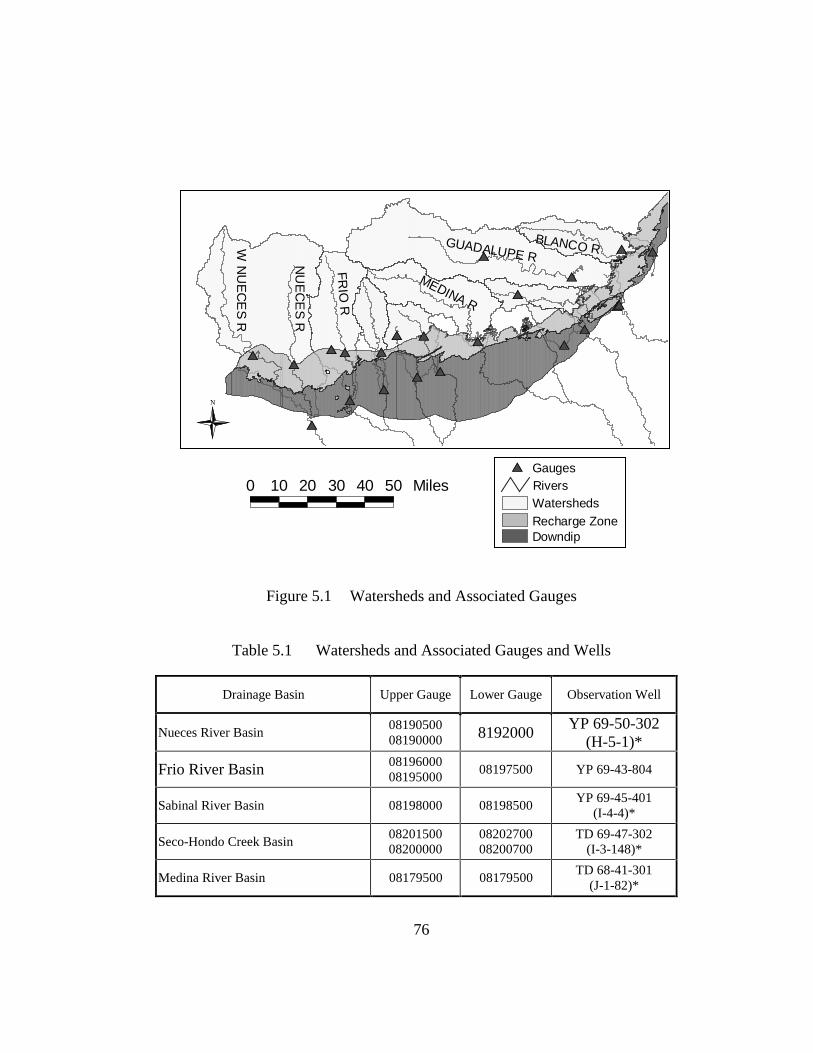
76
�6�6
�6
�6�6
�6
�6
�6
�6
�6
�6
�6
�6 �6
�6
�6
�6
�6
�6
�6 �6 �6
FR
IO R
NU
EC
ES
R
GUADALUPE R
MEDINA R
W N
UE
CE
S R
BLANCO R
WatershedsRecharge ZoneDowndip
Rivers�6 Gauges
0 10 20 30 40 50 Miles
N
Figure 5.1 Watersheds and Associated Gauges
Table 5.1 Watersheds and Associated Gauges and Wells
Drainage Basin Upper Gauge Lower Gauge Observation Well
Nueces River Basin 08190500 08190000 8192000
YP 69-50-302 (H-5-1)*
Frio River Basin 08196000 08195000
08197500 YP 69-43-804
Sabinal River Basin 08198000 08198500 YP 69-45-401
(I-4-4)*
Seco-Hondo Creek Basin 08201500 08200000
08202700 08200700
TD 69-47-302 (I-3-148)*
Medina River Basin 08179500 08179500 TD 68-41-301
(J-1-82)*

77
Drainage Basin Upper Gauge Lower Gauge Observation Well
Helotes-Salado Creek Basin 08181400 08178700 AY 68-37-203
(J-17)*
Cibolo-Dry Comal Creek Basin 08183900 08185000 DX 68-23-302
(G-49)*
Guadalupe River Basin 08167000 08167500
08168500 08169000
Blanco River Basin 08171000 08171300 LR 67-09-110
* Old Well Number
The tank model simulates the flow of water through the aquifer using the
fundamental principles of continuity and momentum. The governing equation for
a tank is
∑ −−−=⋅ )( 21 hhTPRdt
dhS (5.1)
where R is recharge, P is pumpage, S is storativity, T is transmissivity, and h1 and
h2 are the water levels in the tank and the next tank downstream as shown in
Figure 5.3. This equation is discretized over a monthly time step and individual
tanks. The hydraulic properties, storativity and transmissivity, are dependent on
water levels. Consequently, their values change throughout the simulation. This
results in a non-linear, non-stationary system. Recharge is predicted from surface
flows and pumpage is estimated based on monthly pumping data from 1978-1989.
The model is developed in more detail in Section 5.4.
5.2 WATER MOVEMENT
The Edwards Aquifer receives the majority of its recharge through channel
losses in rivers and streams. There are three river basins that pass through the
study area. These are the Nueces, San Antonio, and Guadalupe Rivers. The

78
Nueces River Basin covers over half of the study area and supplies almost 60% of
the recharge to the aquifer. In addition to the larger tributaries, there are several
smaller rivers and creeks, including the Blanco, Frio, Medina, and Sabinal Rivers,
and the Seco and Hondo Creeks. These water bodies lose major portions of their
flow to the aquifer through joints, faults, and sink holes. While the principal
direction of surface flow is south and southeast, water lost to the aquifer is
redirected. Within the confined portion of the aquifer, water flows to the north
and northeast. The aquifer discharges flow through several springs, the largest of
which are Comal and San Marcos Springs. Analyses of tritium content in the
spring flows indicate that water may spend up to twenty years traversing the
aquifer (HDR Engineering, Inc., 1993). Figure 5.2 illustrates the movement of
subsurface water.
Figure 5.2 Movement of Water Within the Edwards Aquifer (© Copyright Eckhardt, 1995)

79
There are nine drainage basins that intersect the Edwards Aquifer recharge
zone. Eight of the basins are considered by the model. Although the Guadalupe
River crosses the infiltration area, seepage studies have indicated that its recharge
contribution is minimal (Puente, 1978). The other watersheds are conceptualized
as a series of rock-filled tanks. The tanks are connected according to the flow
pattern within the aquifer. Channel losses from streams and rivers are assumed to
enter a tank and flow directly to the next tank. The only outlets considered are
Comal and San Marcos Springs. Flow patterns and the configuration of tanks are
shown in Figure 5.3.
Figure 5.3 Tank Configuration (© Copyright Wanakule and Anaya, 1993)
In addition to the natural discharge of water through spring flows, the
Edwards Aquifer also loses water from pumping. Pumping affects water levels
within the formation which, in turn, affects spring flows. Pumping rates are taken
as a fixed output in the tank model. Pumpage data for the period between 1978
and 1989 were provided by the Texas Water Development Board (TWDB).
Analysis of the data provides some insights regarding pumping’s effects on water

80
availability. During 1989, a record high 542,400 AF of water was pumped from
the aquifer. The USGS estimates that the aquifer receives an annual recharge of
651,700 AF (Wanakule and Anaya, 1993). Pumping rates are greatest in the
eastern portion of the region, where the water is mainly used for municipal
purposes. In addition, a large seasonal demand for water is observed in the
western areas, where the water is used in agriculture. As it stands, the model does
not include a mechanism for testing pumping scenarios. However, modification
of the program for these purposes would be relatively simple. For example, the
observed pumping rates could be reduced by a percentage if water levels dropped
below specific requirements. The exploration of management alternatives is
becoming a necessity as pumping rates approach the rate of natural recharge to
the Edwards Aquifer.
5.3 RECHARGE FUNCTIONS
The recharge functions used by the tank model provide a mechanism for
simulating the interactions between surface water and groundwater. Recharge to
the Edwards Aquifer is derived primarily from channel losses in rivers and
streams that flow over the outcrop area. Consequently, recharge estimation
methods have historically focused on measured streamflows at locations above
and below the recharge zone. The amount of recharge can be inferred by using
the following mass-balance equation,
R = QU + QI - QL (5.2)
where QU and QL are upper and lower gauged streamflows, respectively, and QI is
the intervening runoff from precipitation.

81
Much like recharge, intervening runoff is difficult to quantify and must be
estimated. Two methods have been previously used for this purpose. The
standard USGS method assumes that rainfall and runoff conditions are the same
in the recharge zone as they are in the catchment area above the upper gauge
(Puente, 1978). Based on this assumption, the intervening runoff is calculated
using a scaling factor based on the ratio of the intervening area (AI) to the
catchment area (AU),
Q QA
AI UI
U
= ⋅ (5.3)
The inflow values used to calibrate the soil-water balance model are the
sum of upper gauged streamflows and intervening runoff. The intervening runoff
is calculated using the USGS method described above. Instead of assuming that
the estimated intervening runoff is accurate and simply subtracting lower gauged
streamflows to obtain recharge, Wanakule and Anaya (1993) developed empirical
functions by plotting inflow against recharge ratios defined by,
IU
LIU
QQQ
Inflow
RechargeRR
+−+
== (5.4)
where RR is a recharge ratio. Recharge can be estimated without measured
streamflows at the downstream gauge using the following equation: R = RR · Inflow (5.5)
Wanakule and Anaya (1993) developed recharge functions for each
drainage basin using regression analysis with observed data. Their analysis
indicated that as streamflow decreases, the volume of recharge decreases, but the

82
percentage of streamflow lost increases. During dry periods, sometimes flow at
an upper gauge is completely lost to the aquifer (RR = 1), and there is no flow at
the lower gauge. In most cases the recharge ratio is calculated using a non-linear
relationship based on inflows but in some basins, water level was also considered
due to the presence of a shallow water table. Recharge in the Medina River basin
is estimated using a completely different method because of Medina Lake. In this
area, recharge to the aquifer is supplied by seepage losses. Recharge is calculated
based on the volume of water contained in Medina Lake. The derivation of
functions used to estimate recharge is described in more detail in Wanakule and
Anaya (1993). For this study, their functions are used without modification.
5.4 METHODOLOGY
The tank model is used to simulate the movement of water for the
Edwards Aquifer. Its primary function is to estimate flows into and out of a given
tank during a monthly time step. The concepts that form the basis of mass
transfer mechanisms are illustrated in Figure 5.4, which depicts a series of three
connected tanks with piezometric heads that coincide with water levels in
observation wells for separate drainage basins.
Figure 5.4 Groundwater Transport Simulated with a Tank Model

83
The variables shown in Figure 5.4 are piezometric head (h), recharge (R),
pumping (P), transmissivity (T), and the storage coefficient (S).
Groundwater movement is simulated based on the laws of continuity and
momentum. According to the law of mass conservation, the flow into a tank must
equal the flow out of a tank. If the system is not at steady-state, the change in the
volume of water stored in a tank must also be considered. Assuming an
incompressible fluid, the continuity equation can be written as,
Q QV
tin out− =
∂∂
(5.6)
where Qin is the volume of water flowing into a tank, Qout is that flowing out of a
tank, and ∂∂V
t is the change in volume of water stored with time (Wang and
Anderson, 1982).
The water flowing into a tank may be underflow from another tank or
recharge. The tank may lose water to pumping, spring flows, or underflow.
Flows between tanks are controlled by their water levels, also known as heads.
According to Darcy’s Law, water will flow in the direction of decreasing
potential, as given by Q12 = -T · (h1 – h2) (5.7)
where T, the transmissivity, is directly related to hydraulic conductivity, and h1
and h2 are the water levels in the tank and its adjoining neighbor. The negative
sign in this equation indicates that the volume of water in tank one will decrease if
it has a higher potential than tank two.
In addition to being tank dependent, water level is also time dependent.
To account for transient conditions, the rate of release of water from tank storage

84
must be estimated. The rate of release is dependent on the potential for flow. The
storage coefficient is used to characterize the behavior of an element given a head
gradient,
SV
dh=
∂ (5.8)
where ∂V
dh is the change in volume of water stored with a given head differential.
The rate of release from storage can therefore be written as,
dV
dtS
h
dt= ⋅
∂ (5.9)
The following equations were formulated for the tank model by Wanakule
and Anaya (1993). Storativity and transmissivity are the only parameters used to
characterize the hydraulic properties of the system. They are both dependent on
water levels. Transmissivity is calculated using the equation,
T Kh h
T= ⋅+( )1 2
2 (5.10)
where KT is a parameter used to calibrate the model. Thus, transmissivity is a link
characteristic that is based on the average water levels in adjoining tanks. The
function used by the model to calculate storativity is given by, S = KS · n · h1
(n-1) (5.11)
where KS and n are parameters used to calibrate the model. The storativity
parameter is associated with an individual tank.
Watkins (1997) modified the program to solve Aquifer flow equations are
using a form of finite-difference method based on Gauss-Seidel iteration and
Successive Over Relaxation (SOR). The problem is discretized over time and

85
space by determining the movement of water for a single tank over a monthly
time step.
A mass balance equation can be formulated for a tank by considering the
transfer of water between tanks and changes in storage during each time step. By
also accounting for recharge and pumping, the continuity equation for two
adjacent tanks is,
S h h T h h T h h R Pit
it
it
it
it
it
it
it⋅ − = ⋅ − + ⋅ − + +−
−− −
+− − − −[ ] ( ) ( )1
11 1
11 1 1 1 (5.12)
where i is the tank index and t is the time index. This equation can be rearranged
to solve for the water level in the selected tank,
hS
S h T h h T h h R Pit
it
it
it
it
it
it
it= ⋅ ⋅ + ⋅ − + ⋅ − + +−
−− −
+− − − −1 1
11 1
11 1 1 1[ ( ) ( ) ] (5.13)
In the actual program, the general tank equation is modified to account for
boundary conditions and spring flows. If the adjoining tank (i-1) is actually a
boundary, the value of hit−−11 is represented by the linear equation
h hit
i i it
−− −= + ⋅1
1 1α β (5.14)
where α and β are calibration parameters. A constant flux boundary is
simulated by setting αi = 0 , and a constant head boundary is simulated by setting
βi = 0. Spring flows are also modeled by using a linear relationship. If the
adjoining tank (i+1) is actually a spring, the third term on the right-hand side of
the mass balance equation is modified in the following manner,
T h h SprK h SprElevit
it
i it
i⋅ − = − ⋅ −+− − −( ) ( )1
1 1 1 (5.15)
where SprK is a calibration coefficient relating spring flow to water level in a tank
and SprElev is the spring elevation (ft.) (Ye, 1996). The term is negative,

86
indicating that the tank loses water if its water level exceeds the elevation of the
spring.
The tank model repeats the procedure below for each tank and each time
step:
1. Read in initial water levels, stream flows, and pumping rates 2. Read in tank parameters
3. Set h hit
it= −1
4. Calculate T’s based on hit , hi
t−1 , and hi
t+1
5. Calculate S based on hit
6. Calculate R based on streamflows and hit (recharge function)
7. Calculate Spring flows based on hit
8. Calculate a revised hit using tank continuity equation.
9. If the difference between new hit and old hi
t > 0.1 then go to 4.
The groundwater simulation program was calibrated by Watkins (1996).
The program is run in this research without modification using previously
compiled data sets for initial water levels, pumping rates, and tank parameters.
Documentation for the program is provided in Watkins (1996). A data set of
simulated streamflows is created using calculated values from the soil-water
balance program. The groundwater model is then run with the simulated
streamflow data and with observed streamflow data that was collected by
Wanakule and Anaya (1993). The results from these runs are compared in the
next section.
5.5 RESULTS
The groundwater model was run with observed streamflow data, as well as
predicted values from the soil-water balance model. The objective was to

87
evaluate whether aquifer water levels and spring flows predicted using climate-
modeled streamflows are comparable to those predicted using actual
measurements. The accuracy of the predicted values was evaluated by comparing
them to well data provided by the Texas Natural Resource Conservation
Commission (TNRCC) and spring flow data from USGS. The groundwater
model predictions were relatively accurate compared to measured aquifer water
levels and spring flows for the period between 1975 and 1990. Using the
observed streamflows as input achieved an average R-squared of 0.80. The
streamflows predicted by the soil-water balance resulted in an average R-squared
of 0.70. This is notable, considering that the aggregate R-squared value for the
streamflows predicted by the soil-water balance was 0.42. The reason for the
major difference in the level of accuracy stems from the fact that runoff is
strongly influenced by random storm events while aquifer water levels are not.
Changes in the amount of water stored in the formation are more gradual due to
slower hydraulic response times. The relative influence of precipitation on
streamflows and water levels is illustrated in Figure 5.5.

88
0.00
10.00
20.00
30.00
40.00
50.00
60.00
70.00
80.00
90.00
100.00
Jan-75 Jul-77 Jan-80 Jul-82 Jan-85 Jul-87 Jan-90
Stre
am F
low
(1,
000
AF
/mon
th)
Pre
cipi
tati
on(m
m/m
onth
)
700.0
720.0
740.0
760.0
780.0
800.0
820.0
840.0
860.0
880.0
900.0
Wat
er L
evel
(fe
et)
Precipitation Stream Flow Water Level
Figure 5.5 Relationship Between Precipitation, Streamflows and Water Levels for the Nueces River Basin
The straight lines are included to highlight the increasing trends in
streamflows and water levels caused by changes in precipitation. Water levels
also indicate a time lag between climate forcing and aquifer response. This delay
would probably be more apparent if values were available on a daily time-scale.
However, the relatively short delay time can be attributed to the karst
characteristics of the Edwards Aquifer. In alluvial aquifers, the effects of climate
change would be more gradual, and less apparent.
As discussed in Chapter 4, the soil-water balance model tended to under-
predict streamflows to a small degree, even when a modeling constraint was
included to ensure that the total difference between observed and predicted
streamflow values approached zero. This trend was reflected in the water levels

89
and spring flows predicted by the groundwater model. These trends are apparent
in Figures 5.6 and 5.7, which show the observed and predicted water levels of the
Edwards Aquifer in proximity to the Nueces River Basin and the Helotes-Salado
Creek Basin, respectively.
820
830
840
850
860
870
880
890
900
Jan-75 Jul-77 Jan-80 Jul-82 Jan-85 Jul-87 Jan-90
Wat
er L
evel
(fe
et)
Predicted-Known Inflow Predicted-Soil Balance Observed
Figure 5.6 Nueces River Basin: Observed and Predicted Water Levels

90
620
630
640
650
660
670
680
690
700
Jan-75 Jul-77 Jan-80 Jul-82 Jan-85 Jul-87 Jan-90
Wat
er L
evel
(fee
t)Predicted-Known Inflow Predicted-Soil Balance Observed
Figure 5.7 Helotes-Salado Creek Basin: Observed and Predicted Water Levels
The Nueces River Basin water levels are somewhat higher than those for
the Helotes-Salado Creek Basin. Both of the figures were placed on relative
scales to show fluctuations in water levels during the period of record. The region
encompassing the Helotes-Salado Creek Basin is heavily pumped to provide
municipal water supply for San Antonio. Human influence may be a factor in the
increased level of variability in water levels. The potential for recharge increases
during periods when the aquifer is depleted, as evidenced by the increased
percentage of channel losses that occur during dry periods. According to this
hypothesis, climate effects would be magnified by increased pumping of the
aquifer. When rainfall is low for an extended duration, changes in aquifer levels
are more a reflection of pumping rates. The recharge potential, however,

91
increases during this time. When wet climate conditions return, the aquifer
receives more recharge and water levels are quickly replenished.
Increased pumping has had a marked effect on spring flows in the
Edwards region. Comal and San Marcos Springs, the largest springs in Texas,
have experienced decreased flow rates. Some of the smaller springs that once had
continuous flows are now intermittent. San Antonio and San Pedro Springs,
which are located in San Antonio, now stop flowing on a regular basis during
certain parts of the year. Spring flows predicted with observed and climate-based
streamflows are plotted against actual values for Comal Springs in Figure 5.8.
0
5
10
15
20
25
30
35
Jan-75 Jul-77 Jan-80 Jul-82 Jan-85 Jul-87 Jan-90
Spri
ng F
low
(10
00 A
F/m
onth
)
Simulated-Known Inflow Predicted-Soil Balance Observed
Figure 5.8 Comal Springs: Observed and Predicted Spring Flows
The figure clearly shows lower spring flow estimates resulting from the
soil-water balance predicted streamflows. However, the model slightly over-
predicted spring flows when observed streamflows were used as input. A

92
decreasing trend in actual spring flows is also evident. Like spring flows, aquifer
water levels have been reduced by increased pumping. Figure 5.9 shows pumping
rates and observed water levels for the Helotes-Salado Creek Basin near San
Antonio from January, 1975 to September, 1990.
620
630
640
650
660
670
680
690
700
Jan-75 Jul-77 Jan-80 Jul-82 Jan-85 Jul-87 Jan-90
Wat
er L
evel
(fe
et)
12
13
14
15
16
17
18
19
20
Pum
ping
(1,
000
AF
/mon
th)
Water Level Pumping
Figure 5.9 Relationship Between Pumping Rates and Water Levels for the Helotes-Salado Creek Basin
This chapter has discussed climatological and anthropogenic influences on
the Edwards Aquifer. Chapter 6 will examine the effects of altered climate
forcing using scaling factors for precipitation and temperature under 1xCO2 and
2xCO2 scenarios.

93
Chapter 6: Climate Change
Global mean temperatures have increased significantly during the last
century. Projected growth of emission rates for greenhouse gases, primarily
carbon dioxide (CO2), will contribute to a temperature rise of 1.5° to 4.5°C by the
year 2100. The objective of this study is to examine how future changes in
climate will affect water availability in the Edwards Aquifer region. Kittel et al.
(1996) and Valdés (1997) used general circulation models (GCMs) to generate
scaling factors for precipitation and temperature that simulate the impacts of
doubled atmospheric concentrations of CO2 (2xCO2) on regional hydrology. The
concentration of CO2 is doubled relative to global averages observed in 1990.
Climate models provide a physically-based prediction of how precipitation,
temperature and other factors could change under 2xCO2 conditions. Scaling
factors from seven different GCMs are applied to observed climate data and
changes in streamflows are predicted using the soil-water balance program.
Subsequently, the groundwater model is run using the modified streamflows.
This chapter discusses how climate change will influence streamflows, water
levels, and spring flows in the study area.
6.1 METHODOLOGY
Scaling factors for precipitation and temperature are provided by VEMAP
(Kittel et al., 1996) and Valdés (1997). The scaling factors were derived from the
results of GCM runs conducted under normal atmospheric CO2 concentrations
(1xCO2) and 2xCO2 conditions and specify change ratios for precipitation

94
(P2xCO2/P1xCO2) and differences for temperature (T2xCO2-T1xCO2) in °C. Climate
change scenarios represent a possible future in which the atmospheric
concentration of CO2 is instantaneously doubled relative to 1990 levels and
climate is then allowed to reach a new equilibrium (CSIRO 1996). The estimated
values of precipitation, temperature, and other variables under altered CO2
conditions are generated by GCMs for geographic locations on an evenly spaced
grid. These values are then compared to their historical averages (1895-1993).
Temperature scaling factors are calculated by subtracting the historical mean from
the GCM-generated value at a particular point. Precipitation scaling factors are
calculated by dividing the GCM-generated value by the historical average.
Scaling factors are essentially measures of climate sensitivity to modified
atmospheric concentrations of CO2.
VEMAP provided 2xCO2 scaling factors for precipitation and temperature
on a monthly, seasonal, and annual basis. For this study, only the annual scaling
factors are used. In the future, other researchers will most likely expand this work
to include monthly and seasonal scaling factors. The seven GCMs that are
considered are listed below:
• Canadian Climate Centre (CCC) (Boer et al., 1992)
• Goddard Institute for Space Studies (GISS) (Hansen et al., 1984)
• Geophysical Fluid Dynamics Laboratory (GFDL)
− R15 runs without Q-flux corrections (Manabe and Wetherald, 1987)
− R15 runs with Q-flux corrections (Manabe and Wetherald, 1990, Wetherald
and Manabe, 1990)

95
− R30 runs with Q-flux corrections (Manabe and Wetherald, 1990, Wetherald
and Manabe, 1990)
• Oregon State University (OSU) (Schlesinger and Zhao, 1989)
• United Kingdom Meteorological Office (UKMO) (Wilson and Mitchell,
1987)
Two sets of scaling factors were provided for use in this work. Valdés
(1997) provided the results from GFDL R30 10-year equilibrium simulations for
1xCO2 and 2xCO2 scenarios. In addition, results were obtained from the VEMAP
Phase I database for each of the seven climate models (Kittel et al., 1996). Rather
than just using the single set of scaling factors generated by the GFDL R30 10-
year simulation runs, results from all of the GCMs provided by the VEMAP
Phase I database are considered. Seven sets of scaling factors are used to examine
the range of model variability in predicting streamflows, water levels, and spring
flows. Differences for temperature predicted by the seven GCMs are shown in
Figure 6.1 and change ratios for precipitation are shown in Figure 6.2. Values of
the scaling factors for temperature are provided in Table 6.1 and those for
precipitation are provided in Table 6.2.

96
0
1
2
3
4
5
6
7
CCC GISS GFDL R15w/o Q-flux
GFDL R15with Q-flux
GFDL R30 OSU UKMO
Sca
ling
Fac
tor
for
Tem
per
atu
re (
T2-
T1)
[C
]
Figure 6.1 Annual Scaling Factors for Temperature from GCMs
0
0.2
0.4
0.6
0.8
1
1.2
1.4
1.6
1.8
CCC GISS GFDL R15w/o Q-flux
GFDL R15with Q-flux
GFDL R30 OSU UKMO
Sca
ling
Fac
tor
for
Pre
cip
itat
ion
(P
2/P
1)
Figure 6.2 Annual Scaling Factors for Precipitation from GCMs

97
Table 6.1 Annual Scaling Factors for Temperature (ºC)
GCM Temp (T2-T1) CCC 5.953 GISS 2.700 GFDL R15 w/o Q-flux 4.223 GFDL R15 with Q-flux 3.927 GFDL R30 3.753 OSU 4.305 UKMO 3.318 AVERAGE 3.704 AVERAGE w/o R30 4.071
Table 6.2 Annual Scaling Factors for Precipitation
GCM Precip (P2/P1) CCC 0.943
GISS 0.931
GFDL R15 w/o Q-flux 1.152
GFDL R15 with Q-flux 0.990
GFDL R30 1.570
OSU 0.959
UKMO 1.002
AVERAGE 1.078
AVERAGE w/o R30 0.996
The average increase in temperature predicted by the models is 4°C with a
range from 2.7 to 6.0°C. The average change ratio for precipitation is 1.08 with a
range from 0.93 to 1.57. The precipitation scaling factor from GFDL R30 is
considerably higher than those obtained from the other models. If GFDL R30
scaling factors are omitted from the calculation of the mean, the temperature
increase is 3.7°C with a range from 2.7 to 6.0°C and the average change ratio for
precipitation drops to 1.00 with a range from 0.93 to 1.15. The models produced
varying results regarding climate variability. For example, while all of the models

98
predicted increased temperature, mixed results were obtained for precipitation. In
general, GCMs predict temperature changes more accurately than changes in
rainfall. According to Valdés (1997), greater seasonal variability in rainfall is
forecast by the models. Precipitation tends to increase in the summer and
decrease in the spring. Rainfall decreases more frequently in the study region, but
extreme wet conditions may also occur. Although monthly and seasonal
variability is not considered in predicting streamflows, spring flows, and water
levels, it affects annual scaling factors, producing mixed results for rainfall
change ratios. Sub-annual variability causes average annual change ratios to be
greater than unity for three of the models. The differences provided for each of
the seven GCMs are applied to historical time series for temperature, and
precipitation data are multiplied by change ratios. The soil-water balance
program and groundwater model are then run using the modified data sets.
Trends in water availability for 1xCO2 and 2xCO2 conditions under normal and
increased pumping scenarios are discussed in the next section.
6.2 RESULTS
The soil-water balance program was modified to allow the user to specify
scaling factors for precipitation and temperature. Three different versions of the
program are included in Appendix B. These versions are used for calibration,
validation, and climate change modeling. Using the third version, the program
was run with annual average scaling factors from seven different GCMs. After
completing the seven model runs, it was determined that the variability in
streamflows predicted with 2xCO2 climate factors covered a consistent range of

99
outcomes. The GFDL R30 scaling factors produced streamflows that were
significantly higher than those predicted by the other models. In contrast, the
streamflows predicted using CCC scaling factors were always lower relative to
the results from the other simulations. The ratios of average streamflows from
1975-1990 predicted under 2xCO2 climate scenarios to the 1xCO2 average for the
Nueces River Basin in Figure 6.3. Values of the average ratios (2xCO2/1xCO2)
for streamflow are provided in Table 6.3.
0.0
0.5
1.0
1.5
2.0
2.5
CCC GISS GFDL R15w/o Q-flux
GFDL R15with Q-flux
GFDL R30 OSU UKMO
Mea
n S
trea
mfl
ow
197
5-19
90 (
Q2/
Q1)
Average - 1xCO2
Figure 6.3 Average Streamflow Scaling Factors for the Nueces River Basin from 1975-1990 Predicted from GCM Climate Scenarios

100
Table 6.3 Annual Scaling Factors for Streamflow in the Nueces River Basin
GCM Flow (Q2/Q1) CCC 0.597
GISS 0.711
GFDL R15 w/o Q-flux 1.017
GFDL R15 with Q-flux 0.750
GFDL R30 2.034
OSU 0.684
UKMO 0.800
AVERAGE 0.942
AVERAGE w/o R30 0.760
As shown in Figure 6.3, all of the scaling factors except those for GFDL
R30 predicted streamflows that were at or below the average for the 1975 to 1990
period under a 1xCO2 scenario. Average streamflows dropped from 16,700
AF/month under normal climate conditions to 10,000 AF/month predicted by the
CCC model. The average change ratio for streamflow predicted by the models is
0.94 with a range from 0.60 to 2.0; omitting the GFDL R30 results reduces the
average to 0.76 and the range varies from 0.6 to 1.0. Climate change essentially
forces a redistribution of water resources for the area. Higher temperatures cause
more evaporation losses. If these losses are not supplemented by rainfall, runoff
decreases. Streamflow trends are more closely correlated with precipitation
change ratios than with predicted temperature differences. The unusual results
from the GFDL R30 runs are caused by a simulated 57% increase in precipitation.
Modified streamflow data sets from the 2xCO2 scaling factor runs were
used as input to the groundwater model to identify trends in aquifer responses to
climate change. Model variability in predicted water levels and spring flows

101
followed the same trends observed in the soil-water balance program. Figure 6.4
shows average water levels for the Nueces River Basin from 1975-1990 and
Figure 6.5 shows these results for the Helotes-Salado Creek Basin. Table 6.4
provides the average change in water levels (ft.) for the Nueces River Basin and
the Helotes-Salado Creek Basin from 1975-1990 compared to the annual average
for 1975.

102
830
840
850
860
870
880
890
CCC GISS GFDL R15w/o Q-flux
GFDL R15with Q-flux
GFDL R30 OSU UKMO
Mea
n W
ater
Lev
el 1
975-
1990
(ft
)Average - 1xCO2
Figure 6.4 Average Water Levels for the Nueces River Basin from 1975-1990 Predicted from GCM Scaling Factors
620
630
640
650
660
670
680
C C C G ISS G F D L R 15w /o Q -flux
G FD L R 15w ith Q -flux
G FD L R 30 O SU U KM O
Mea
n W
ater
Lev
el 1
975-
1990
(ft
)
Average - 1xC O 2
Figure 6.5 Average Water Levels for the Helotes-Salado Creek Basin from 1975-1990 Predicted from GCM Scaling Factors

103
Table 6.4 Average Change in Water Levels (ft.) from 1975 to 1990
GCM
Nueces Average=880.7 ft.
Helotes-Salado Average=679.4 ft.
CCC -56.9 -53.1 GISS -44.3 -47.6 GFDL R15 w/o Q-flux -20.3 -36.1 GFDL R15 with Q-flux -40.0 -45.4 GFDL R30 -1.6 -15.9 OSU -47.1 -48.7 UKMO -35.6 -43.3 AVERAGE -35.1 -41.5 AVERAGE w/o R30 -40.7 -45.7 1xCO2 -20.3 -36.1
The water levels for the Nueces River Basin are measured using USGS
observation well YP 69-50-302, which was formerly numbered H-5-1. Since the
Edwards Aquifer gets nearly 60% of its recharge from the Nueces River Basin,
these results are indicative of variability in water supply under 2xCO2 conditions.
Higher average water levels correspond to higher streamflows and spring flows.
The average decrease in water levels under 2xCO2 for the Nueces Basin (1975-
1990) is 35.1 ft. The water levels for the Helotes-Salado Creek Basin are
measured by observation well AY 68-37-203, which was formerly numbered J-
17. Comal Springs become intermittent when the level of the J-17 well drops
below 620 ft. (Eckhardt, 1995). The average water levels predicted using the
seven different GCM scaling factors are higher than 620 ft. However, water
levels fall below 620 ft. temporarily during the modeled time period (Figure 6.7).
The average decrease in water levels under 2xCO2 climate scenarios for the
Helotes-Salado Creek Basin is 41.5 ft. Figure 6.6 illustrates water level
variability over time under 1xCO2 and 2xCO2 for the Nueces River Basin. These

104
results are presented for the Helotes-Salado Creek Basin in Figure 6.7. The lines
representing the results from different GCM scaling factors are placed in order
from highest to lowest average water levels. The results for normal (1xCO2)
climate conditions are depicted with a heavier line. Water level variability
predicted by the scaling factors from GFDL R15 without Q-flux corrections is
very similar to that for 1xCO2 conditions. Consequently, this line is hard to
differentiate from the heavier line for normal climate conditions.
800
810
820
830
840
850
860
870
880
890
900
Jan-75 Jul-77 Jan-80 Jul-82 Jan-85 Jul-87 Jan-90
Wat
er L
evel
(ft
)
1xCO2
R30
R15
UKMO
R15 w/Q
GISS
OSU
CCC
Figure 6.6 Water Level Variability for the Nueces River Basin from 1975-1990 Predicted from GCM Scaling Factors (Legend Ordered by Decreasing Average Water Level)

105
600
610
620
630
640
650
660
670
680
690
700
Jan-75 Jul-77 Jan-80 Jul-82 Jan-85 Jul-87 Jan-90
Wat
er L
evel
(ft
)
1xCO2
R30
R15
UKMO
R15 w/Q
GISS
OSU
CCC
Figure 6.7 Water Level Variability for the Helotes-Salado Creek Basin from 1975-1990 Predicted from GCM Scaling Factors (Legend Ordered by Decreasing Average Water Level)
Water levels predicted using GFDL R30 scaling factors were noticeably
offset from the other model results. Six out of the seven GCMs predicted water
levels at or below those observed under normal climate conditions. Since the
GFDL R30 results do not agree with trends predicted by the other models, and
because a 57% increase in precipitation is somewhat questionable, subsequent
figures do not include statistics from this particular model. However, the results
are considered to be significant, in that water availability in the Edwards region
could increase given the possibility of a substantial increase in future rainfall.
The range of outcomes for water levels from the majority of the GCMs

106
considered in this study is shown for the Nueces River Basin in Figure 6.8 for the
Helotes-Salado Creek Basin in Figure 6.9, and for the Blanco River Basin in
Figure 6.10. The shading that represents model variability extends slightly above
the line for 1xCO2 conditions in all cases. This is difficult to differentiate because
the second highest water levels, predicted by the GFDL R15 model, approximate
those forecast for normal climate conditions.
800
810
820
830
840
850
860
870
880
890
900
Jan-75 Jan-80 Jan-85 Jan-90
Wat
er L
evel
(ft
)
Model Variability 1xCO2
GFDL R15
CCC
Figure 6.8 Range of Water Level Predictions for the Nueces River Basin

107
600
610
620
630
640
650
660
670
680
690
700
Jan-75 Jan-80 Jan-85 Jan-90
Wat
er L
evel
(ft
)
model variability 1xCO2
GFDL R15
CCC
Figure 6.9 Range of Water Level Predictions for the Helotes-Salado Creek Basin
500
510
520
530
540
550
560
570
580
590
600
Jan-75 Jan-80 Jan-85 Jan-90
Wat
er L
evel
(ft
)
Model Variability 1xCO2
GFDL R15
CCC
Figure 6.10 Range of Water Level Predictions for the Blanco River Basin
108
The effects of climate change appear to grow over time for the Nueces
River Basin and the Helotes-Salado Creek Basin. However, the Blanco River
Basin showed a very limited response to modified climate forcing under 2xCO2
conditions. Faulting and complex flow patterns cause some portions of the
formation to exhibit greater variability in water levels. In general, regions with
lower water level variability are less susceptible to climate change. This is also
true for spring flows. San Marcos Springs are not as sensitive as Comal Springs
to changes in aquifer water levels. San Marcos Springs receive a large portion of
their water supply from local sources of recharge. Comal Springs, on the other
hand, are recharged by water originating from farther reaches of the aquifer, as
evidenced by analyses of tritium content. Tritium levels in spring flows are
indicative of the amount of time the water spent in the subsurface. Comal Springs
flows are highly correlated to fluctuations in observed water levels in observation
well J-17 (Helotes-Salado Creek Basin). Figure 6.11 compares average spring
flows from 1975-1990 predicted under 2xCO2 climate scenarios with the 1xCO2
average for Comal Springs. These results are presented for San Marcos Springs
in Figure 6.12. Values of the average ratios (2xCO2/1xCO2) for Comal and San
Marcos Springs are presented in Table 6.5 and Table 6.6, respectively.

109
0.0
0.2
0.4
0.6
0.8
1.0
1.2
1.4
1.6
CCC GISS GFDL R15w/o Q-flux
GFDL R15with Q-flux
GFDL R30 OSU UKMO
Mea
n S
pri
ng
Flo
w 1
975-
1990
(Q
2/Q
1) Average - 1xCO2
Figure 6.11 Average Scaling Factors for Spring Flows from Comal Springs Predicted from GCM Climate Scenarios (1975-1990)
0.0
0.2
0.4
0.6
0.8
1.0
1.2
1.4
CCC GISS GFDL R15w/o Q-flux
GFDL R15with Q-flux
GFDL R30 OSU UKMO
Mea
n S
pri
ng
Flo
w 1
975-
1990
(Q
2/Q
1)
Average - 1xCO2
Figure 6.12 Average Scaling Factors for Spring Flows from San Marcos Springs Predicted from GCM Climate Scenarios (1975-1990)

110
Table 6.5 Annual Scaling Factors for Spring Flows from Comal Springs
GCM Flow (Q2/Q1)) CCC 0.579 GISS 0.718 GFDL R15 w/o Q-flux 1.000 GFDL R15 with Q-flux 0.762 GFDL R30 1.424 OSU 0.692 UKMO 0.819 AVERAGE 0.856 AVERAGE w/o R30 0.762
Table 6.6 Annual Scaling Factors for Spring Flows from San Marcos Springs
GCM Flow (Q2/Q1)) CCC 0.818 GISS 0.878 GFDL R15 w/o Q-flux 0.999 GFDL R15 with Q-flux 0.894 GFDL R30 1.290 OSU 0.864 UKMO 0.917 AVERAGE 0.951 AVERAGE w/o R30 0.895
The majority of GCMs predicted decreased spring flows under 2xCO2
climate scenarios. Omitting the results from GFDL R30, the average change ratio
for spring flow from Comal Springs is 0.76 with a range from 0.58 to 1.00.
Average spring flows for Comal Springs dropped from 14,400 AF/month under
normal climate conditions to 8,300 AF/month predicted by the CCC model. San
Marcos spring flows had a weaker response, dropping by 1,400 AF/month, using
CCC scaling factors. The average change ratio for spring flow from San Marcos
Springs, without considering GFDL R30, is 0.90 with a range from 0.82 to 1.00.

111
The GFDL R30 model predicted significantly higher streamflows in the future.
The range of outcomes predicted by the majority of GCMs is shown for Comal
Springs in Figure 6.13. The results for San Marcos Springs are shown in
Figure 6.14.
0
5
10
15
20
25
30
Jan-75 Jan-80 Jan-85 Jan-90
Spri
ng F
low
(10
00 A
F/m
onth
)
Model Variability 1xCO2
GFDL R15
CCC
Figure 6.13 Range of Spring Flow Predictions for Comal Springs

112
0
5
10
15
20
25
30
Jan-75 Jan-80 Jan-85 Jan-90
Spri
ng F
low
(10
00 A
F/m
onth
)
Model Variability 1xCO2
GFDL R15
CCC
Figure 6.14 Range of Spring Flow Predictions for San Marcos Springs
The behavior of Comal Springs follow the trend of increased climate
sensitivity given a higher variability in flow rates. However, flow rates from
Comal Springs decrease even under normal conditions. Pumping has had a
negative impact on the amount of water available to the springs. The groundwater
model was run with increased pumping scenarios to examine the effects of
increased pumping on water levels and spring flows. In Chapter 5, observed
decreases in water levels for the Helotes-Salado Creek Basin were shown to be
closely correlated with increased removal of water from the aquifer. A straight
line was fitted to observed pumping rates for this basin to forecast changes over
time. The following equation was used to predict pumping for the year 2000: P Y= ⋅ −0 3285 635. (6.1)

113
where P is predicted pumping (1000 AF/month) and Y is the year. This function
estimates pumping to reach 22,000 AF/month by the year 2000. This is a 35%
increase over average pumping rates in 1975.
An alternate pumping scenario was created by scaling observed pumping
using a constant factor. Since the Helotes-Salado Creek Basin is heavily pumped
to provide drinking water for the growing population of San Antonio, a more
conservative growth rate of 25% was assumed for pumping throughout the
Edwards region during the period from 1975 to 2000. The historical time series
for pumping was multiplied by this scaling factor and the groundwater model was
run under different climate scenarios using the modified data set. The influence
of increased pumping on water levels for index well J-17 (Helotes-Salado Creek
Basin) is shown in Figure 6.15. Figure 6.16 shows spring flows for Comal
Springs predicted for 2xCO2 conditions with increased pumping.
550
560
570
580
590
600
610
620
630
640
650
660
670
680
690
700
Jan-75 Jan-80 Jan-85 Jan-90
Wat
er L
evel
(ft
)
Model Variability 1xCO2
GFDL R15
CCC
Average-Observed Pumping
Average-Pumping Increased by 25%
Figure 6.15 Index Well J-17 Water Levels Predicted Under Increased Pumping

114
0
5
10
15
20
25
30
Jan-75 Jan-80 Jan-85 Jan-90
Spri
ng F
low
(10
00 A
F/m
onth
)
Model Variability 1xCO2
GFDL R15
CCC
Average-Observed Pumping
Average-Pumping Increased by 25%
Figure 6.16 Spring Flows for Comal Springs Predicted Under Increased Pumping
Historical precipitation data for the Edwards area indicate that the last
three decades have had higher than average precipitation (Figure 3.2). Water
levels and spring flows respond to climate change on a much faster time scale,
however. A repeat of the drought of record would most likely have a substantial
negative impact on water resources. Although GCM predictions for precipitation
have a greater level of uncertainty, temperatures will undoubtedly rise over the
next century. Unless increased evaporation is offset by rainfall, significant drops
in water levels would occur during an extended dry period. Moreover, the
Edwards region is experiencing population growth which has led to greater
pumping of the aquifer. As shown in Figures 6.15 and 6.16, the combined effects
of climate change and pumping will severely limit water supply in the study area.
Conclusions are provided in the next chapter.

115
Chapter 7: Conclusions
This conclusion provides a brief summary of the important features of this
study and represents the combined efforts of Dr. David Maidment and myself.
–Kris Martinez, 1998
7.1 SUMMARY OF RESULTS
The objective of this study is to evaluate how climate change would affect
water availability for the Edwards Aquifer region. Surface water and
groundwater models are run under normal and altered climate scenarios which
simulate precipitation and temperature changes under current and doubled
atmospheric concentrations of CO2. The results indicate that gradually rising CO2
levels will bring about a warmer climate in the study region. Higher temperatures
will have a negative impact on water availability, as shown in Table 7.1
Table 7.1 Effects of Climate Change in the Edwards Aquifer Region
Variable Average Low High Annual Temperature (Future – Present) +4.0°C +2.7°C +6.0°C Annual Precipitation Ratio (Future/Present) 1.00 0.93 1.15 Annual Streamflow Ratio (Nueces River) 0.76 0.60 1.00 1975-1990 Water Level (Nueces Basin) -20.4 ft -36.6 ft 0.0 ft 1975-1990 Water Level (Helotes-Salado Basin) -9.6 ft -17.0 ft 0.0 ft Comal Spring Annual Flow Ratio 0.76 0.58 1.00 San Marcos Spring Annual Flow Ratio 0.90 0.82 1.00
The extent of climate change was estimated using General Circulation
Models (GCMs) in a previous study by the National Center for Atmospheric
Research (Jenne, 1992). The study used five different GCMs, developed by
research centers in the United States, Canada, and the United Kingdom, to obtain
116
scaling factors which measure climate sensitivity to CO2 concentrations. There
was a consensus among the models that increased levels of CO2 will produce a
warmer climate in Central Texas with an increase in the mean annual temperature
of approximately 4.0°C (7.2°F) with a range from 2.7 to 6.0°C (4.9 to 10.8°F).
The majority of the GCMs predict normal precipitation. Although rainfall will
remain unchanged, increased temperature will lead to greater evaporation losses
with the end result being a diminished water supply. A temperature increase of
the magnitude predicted by the GCMs would have a marked effect on the
Edwards region.
The results are complicated by the fact that one of the GCMs predicted a
57% increase in rainfall under doubled CO2 concentrations. An experiment by
Manabe and Wetherald (1990) in which the Geophysical Fluid Dynamics
Laboratory (GFDL) R30 model was run with Q-flux corrections produced a
precipitation change ratio of 1.57. Two other experiments using a different
version of the GFDL model (R15) forecast increasing precipitation of up to 15%
[e.g., Manabe and Wetherald (1987) and Manabe and Wetherald (1990)]. The
reason for the large discrepancy between the separate experiments is unclear.
However, when a precipitation change ratio of 1.57 is applied to historical climate
data and the surface and groundwater models are run, the results show a
significantly higher level of water availability in the region. The disparate scaling
factor generated by the GFDL R30 model requires further investigation. The
summary provided in Table 7.1 does not include GFDL R30 predictions.

117
The consequence of a warmer climate is that evaporation is increased and
streamflow is decreased relative to current conditions. Future average flows in
the Nueces River are predicted to be reduced to 76% of their current levels, with a
range from 60-100%. Reduced streamflows lead to reduced groundwater
recharge and thus to reduced aquifer water levels. Water levels in the San
Antonio portion of the aquifer measured by the J-17 Index Well dropped 36 ft
during the 1975-1990 period. Lowered water levels were primarily the result of
increased pumping but model runs indicate that climate change would magnify
these effects, decreasing levels by an additional 10 ft. Over the modeled time
frame, the J-17 water level repeatedly fell below levels associated with
intermittent spring flows for Comal Springs, under altered climate conditions.
The portion of the aquifer in proximity to the Nueces River Basin, measured by
the H-5-1 Index Well, were impacted less by pumping and more by climate
change. Although levels dropped approximately 20 ft during the 1975-1990 time
period, model runs estimate an additional 20 ft decrease would have occurred if
atmospheric concentrations of CO2 were doubled.
The discharges from the two main springs are also reduced. The model
data indicate that mean annual flow in Comal Springs would be reduced to 0.76 of
current levels with a range of 0.58 to 1.00, and that in San Marcos Springs to 0.9
of current levels with a range from 0.82 to 1.00. While there is still a significant
amount of uncertainty surrounding these predictions, the results from all seven of
the GCMs indicate that the Edwards region will experience a much warmer
climate in the future. According to the models, the drying effects of increased

118
temperatures will not be offset by precipitation. As a result, streamflows, aquifer
water levels, and spring flows will be reduced if atmospheric CO2 concentrations
double relative to current levels. This is a significant conclusion because it
suggests that the negative effects of greater water demands in the region will be
magnified by the natural forces of climate change. Further research is necessary
to determine rational alternatives to reconcile the increased need for water to
support human activities with the likelihood of decreased supply.
7.2 STUDY LIMITATIONS
This study has many limitations. The scaling factors that were used to
analyze climate change were annual factors applied uniformly to all months of the
year. A more detailed impact study could use monthly scaling factors derived
separately for each month. A limited historical period from 1975 to 1990 was
used to study effects on the aquifer, because this was the period for which
recorded streamflows were available at all required locations to compare to
simulated values. The climate data developed in this study range from 1895 to
1993, and examination of a longer period is necessary to judge the impacts during
critical periods such as the 1950’s drought. The groundwater model used in this
research is a simplified tank model and more complex and accurate groundwater
models are available, such as the GWSIM IV model from the Texas Water
Development Board (TWDB). A standard approach to estimating groundwater
recharge from streamflow was employed in this study but it is possible that
refinements in this method could lead to improved predictions. A significant
uncertainty in the current study is the degree of discrepancy found between the

119
effects of climate change on precipitation in the region for the GFDL R30 model
and the six other global climate models whose results were used. The reasons for
the changes in precipitation need to be more closely examined and understood.
Perhaps the greatest limitation of this study is that while the evidence for
increasing content of greenhouse gases in the atmosphere is unambiguous,
prediction of how long it will take before the concentration of carbon dioxide
doubles in the atmosphere is quite uncertain. The effects of climate change will
not be felt abruptly, but will be an added effect applied slowly year by year,
whose impact may be difficult to identify independently of the great climatic
variations through time which occur naturally.
7.3 CONTRIBUTIONS
A major accomplishment of this work has been to integrate climate,
surface water, and groundwater modeling. Scaling factors for climate scenarios
are provided by VEMAP (Kittel et al., 1996) and Valdés (1997). The rainfall-
runoff model provided by Reed, Maidment, and Patoux (1997) is modified to use
a temperature-based method for estimating evaporation. This allows the model to
estimate streamflows using precipitation and temperature, which are the only
parameters for which 2xCO2 scaling factors are provided. The groundwater
recharge functions of Wanakule and Anaya (1993) are used for calculating
recharge given streamflows at gauging stations located above the Edwards
Aquifer outcrop. A groundwater model provided by Watkins (1997), which uses
these recharge functions, is employed in this research to provide a mechanism for
estimating water levels and spring flows. The rainfall-runoff model is calibrated

120
to match observed streamflows using historical climate data. The rainfall-runoff
and groundwater models are then run consecutively with normal and altered
precipitation and temperature data to predict streamflows, water levels, and spring
flows. This study successfully links models to describe the influence of climate
on surface and subsurface water availability.
A great deal of information about the Edwards Aquifer has been
assembled within a GIS framework. A digital base map is developed which
includes layers describing climate, terrain, soils, and other meaningful
characteristics. Geographical features, such as cities, counties, roads, and rivers
are also depicted. The base map shows the locations of pertinent gauging
stations, along with Comal Springs and San Marcos Springs. The spatial analysis
capabilities of GIS are used to create an accurate representation of the drainage
basins that provide recharge to the aquifer. A program has been written to
interpolate historical climate data from a 0.5° by 0.5° grid to provide monthly
time-series data for each of the watersheds. Another program has been written to
derive an average soil-water holding capacity for a drainage basin using
STATSGO soils data. All of the programs developed for the study are provided
in Appendix B. A data dictionary is included as Appendix A which describes all
of the information that has been brought together to complete this work.

121
Appendix A Data Dictionary

122
The data dictionary lists the spatial information that was assembled for
this study. Included in the index are coverages, shapefiles, grids, and tables.
Scripts and programs used in the project are contained in Appendix C. The
following conventions are used: Pnt Point Coverage Arc Arc Coverage Ply Polygon Coverage Grd Grid Tbl Table
All coverages and grids are in the Texas Statewide Mapping System
projection, unless otherwise noted.

123
Name Class Attributes Values Description Average Tbl precipitation (mm/month)
temperature (°C) runoff (acre·ft/month) water level (ft)
floating point Average values for basins (1975-1990)
Basins Ply grid code 1 Nueces 2 Frio 3 Sabinal 4 Seco-Hondo 5 Medina 6 Helotes-Salado 7 Cibolo 8 Guadalupe 9 Blanco
Edwards Aquifer watersheds
B_wlvl Tbl water level (ft) floating point Average monthly water levels for basins (1975-1990)
Cities Ply Cities in the study area (polygon)
Citypnt Pnt Cities in the study area (point)
Comp Tbl seqnum integer STATSGO component number
Counties Ply county name Counties in the study area
Edfill2 Grd elevation floating point Digital Elevation Model (DEM) for the study area
Edwards Ply aquifer 0 nodata 1 outcrop 2 downdip
Edwards Aquifer
Gage Pnt gauge number USGS stream gauges
Grid Arc latitude/longitude on 10 minute grid
Huc Ply HUC code USGS Hydrologic Unit Codes (HUCs) major and minor river basins
Latlong Arc latitude/longitude on 5° grid
Layer Tbl water holding capacity (in) floating point Soil-water holding capacity for each layer
Mapunit Tbl muname STATSGO map unit name

124
Name Class Attributes Values Description
Ppttbl Tbl precipitation (mm/month) floating point Average monthly rainfall for basins (1975-1990)
Rainave Tbl precipitation (mm/month) floating point Average rainfall for basins (1975-1990)
Raingrd Ply precipitation (mm/month) integer VEMAP monthly rainfall (1975-1990)
Rivers Arc USGS Reach File 1 (RF1) rivers and streams
Roads Arc Streets and highways Spflwtbl Tbl spring flow
(1000 acre·ft/month) floating point Comal and San
Marcos Springs monthly
Springs Pnt Comal and San Marcos Springs
Statsgo Ply water holding capacity (in) floating point Soil-water holding capacity for each map unit
Surptbl Tbl streamflow (1000 acre·ft/month)
floating point Average monthly streamflow for basins (1975-1990)
Tempave Tbl temperature (°C) floating point Average temperature for basins (1975-1990)
Texas Ply county name Counties of Texas Tmaxtbl Tbl temperature (°C) floating point VEMAP monthly
maximum temperature (1975-1990)
Tmintbl Tbl temperature (°C) floating point VEMAP monthly minimum temperature (1975-1990)
Usgs Ply USGS 1:250,000 quadrangles
Vemap Pnt Centroids of VEMAP grid cells
Wlvltbl Tbl water level (ft) floating point Average monthly water level for basins (1975-1990)

125
Appendix B Programs and Scripts

126
Program Name Language Function
Calbrate.for FORTRAN 77 Calibration version of soil-water balance used to find parameter values that achieve best match between observed and predicted streamflows from August 1982-July 1990 (96 months)
Output.inc FORTRAN 77 Groundwater model sub-program that writes Edwards Aquifer water levels and spring flows to sim.out
Read.inc FORTRAN 77 Groundwater model sub-program used to read in streamflows, pumping rates, initial water levels, and other parameters
Sim.f FORTRAN 77 Groundwater model used to estimate Edwards Aquifer water levels and spring flows given streamflows
ToGrnd.for FORTRAN 77 Final output version of soil-water balance used to write file togrnd.txt to be used as input in groundwater model
Validate.for FORTRAN 77 Validation version of soil-water balance used to check the accuracy of the program against observed streamflows from August 1975-July 1983(96 months)
WHCcalc.ave Avenue Calculates the soil-water holding capacity for each map unit
ZoneMean.ave Avenue Calculates the mean of a value theme variable for each feature in a zone theme

127
Calbrate.for

128
PROGRAM CALIBRATE ! Original program by Reed, Maidment, and Patoux (1997) IMPLICIT NONE REAL P(8,8,13), TMAX(8,8,13), TMIN(8,8,13) REAL STMAX(8), AREA(8) REAL SURP_OBS(8,8,13), SURP_PRD(8,8,13) REAL EVAP_BDG(8,8,13), EVAP_PRD(8,8,13) REAL ST(8,8,13), DST(8,8,13) REAL ST_TEMP, SATUR, DIFF REAL DIST, SIGMA, PHI, OMEGA, PI REAL SORAD, T_AVE, E_POT, EVVAL, EVAPTOT REAL A, C, RC, DSURP, SURPTOT, RUNOFF INTEGER NDAYS(12), D, MNTH, YR, JDAY INTEGER I, K, TANK, TK LOGICAL CONVERGE
! ************************* ! CALIBRATION VARIABLES ! ************************* REAL SMIN, SMAX, SINT, AMIN, AMAX, AINT, S, T REAL N, SUMX, SUMY, SUMXSQ, SUMYSQ, SUMXY, RSQ, NUM, DEN REAL E, ERROR, SUMOBS, BIGDIF, BIGDIFE, BIGDIFR REAL ABESTR, CBESTR, ABESTE, CBESTE, MAXRSQ, MINERR DATA NDAYS /31,30,31,30,31,31,28,31,30,31,30,31/ OPEN(UNIT=10, FILE=’surplus.txt’, STATUS=’old’)
OPEN(UNIT=22, FILE=’input.txt’, STATUS=’unknown’)
! -------------------------------------------------- ! THIS SECTION READS THE INPUT DATA AND THEN WRITES ! IT TO A SINGLE FILE CALLED INPUT.TXT AS A CHECK ! INPUT FILES: SURPLUS.TXT, PPT.TXT, TMAX.TXT, ! TMIN.TXT, STMAX.TXT, AREA.TXT ! OUTPUT FILES: OUTBEST.TXT, OUTCAL.TXT ! --------------------------------------------------
WRITE (22,*) ’--OBSERVED SURPLUS--’ WRITE (22,*) ’’ DO TANK=1,8 WRITE(22,*) ’’ WRITE(22,*) ’TANK:’,TANK DO YR=1,8 READ(10,*) (SURP_OBS(TANK,YR,MNTH), MNTH=1,12) WRITE(22,500) TANK,YR,(SURP_OBS(TANK,YR,I), I=1,12) ENDDO ENDDO

129
500 FORMAT(I2,I2,12(F8.2))
WRITE (22,*) ’’ WRITE (22,*) ’--PRECIPITATION--’
OPEN(UNIT=20, FILE=’ppt.txt’, STATUS=’old’) DO TANK=1,8 WRITE(22,*) ’’ WRITE(22,*) ’TANK:’,TANK DO YR=1,8 READ(20,*) (P(TANK,YR,MNTH), MNTH=1,12) WRITE(22,500) TANK,YR,(P(TANK,YR,I), I=1,12) ENDDO ENDDO
WRITE (22,*) ’’ WRITE (22,*) ’--MAXIMUM TEMP--’ OPEN(UNIT=30, FILE=’tmax.txt’, STATUS=’old’) DO TANK=1,8 WRITE(22,*) ’’ WRITE(22,*) ’TANK:’,TANK DO YR=1,8 READ(30,*) (TMAX(TANK,YR,MNTH), MNTH=1,12) WRITE(22,500) TANK,YR,(TMAX(TANK,YR,I), I=1,12) ENDDO ENDDO
WRITE(22,*) ’’ WRITE(22,*) ’--MINIMUM TEMP--’ OPEN(UNIT=40, FILE=’tmin.txt’, STATUS=’old’) DO TANK=1,8 WRITE(22,*) ’’ WRITE(22,*) ’TANK:’,TANK DO YR=1,8 READ(40,*) (TMIN(TANK,YR,MNTH), MNTH=1,12) WRITE(22,500) TANK,YR,(TMIN(TANK,YR,I), I=1,12) ENDDO ENDDO OPEN(UNIT=50, FILE=’stmax.txt’, STATUS=’old’) DO TANK=1,8 READ(50,*) STMAX(TANK) ENDDO OPEN(UNIT=60, FILE=’area.txt’, STATUS=’old’) DO TANK=1,8 READ(60,*) AREA(TANK)

130
ENDDO CLOSE(10) CLOSE(20) CLOSE(30) CLOSE(40) CLOSE(50) CLOSE(60) CLOSE(22) OPEN(UNIT=51, FILE=’outbest.txt’, STATUS=’unknown’) OPEN(UNIT=61, FILE=’outcal.txt’, STATUS=’unknown’)
WRITE(61, *) ’ C A RSQ & E BIGDIF’ PI=3.1415927
PHI=(29.+58./60.)*PI/180. A=0.0 C=0.0 MINERR = 1000. MAXRSQ = 0.0
PRINT *, ’’ PRINT *, ’*****************************’ PRINT *, ’ENTER CALIBRATION PARAMETERS’ PRINT *, ’MINIMUM,MAXIMUM,STEP INTERVAL’ PRINT *, ’*****************************’ PRINT *, ’’ PRINT *, ’KMIN: ’ READ *, SMIN PRINT *, ’KMAX: ’ READ *, SMAX PRINT *, ’KINT: ’ READ *, SINT PRINT *, ’AMIN: ’ READ *, AMIN PRINT *, ’AMAX: ’ READ *, AMAX PRINT *, ’AINT: ’ READ *, AINT PRINT *, ’STATS FOR TANK: ’ READ *, TK
DO S = SMIN,SMAX,SINT C = S PRINT *, ’’

131
PRINT *, ’K =’, C DO T = AMIN,AMAX,AINT
A = T PRINT *, ’’ PRINT *, ’K =’, C PRINT *, ’A =’, A
DO TANK=1,8 DO YR=1,8 DO MNTH=1,12 SURP_PRD(TANK,YR,MNTH)=0 EVAP_BDG(TANK,YR,MNTH)=0 EVAP_PRD(TANK,YR,MNTH)=0 ST(TANK,YR,1)=0.01 ENDDO ENDDO ENDDO
DO TANK=1,8 DO YR=1,8 CONVERGE=.FALSE. K=0 JDAY=212 ! BEGIN BUDGET LOOP FOR GIVEN TANK DO WHILE (K.LE.30.AND.(.NOT.CONVERGE)) K=K+1 ! INITIALIZE VARIABLES DO MNTH=1,12 ST_TEMP=ST(TANK,YR,MNTH) SURPTOT=0 EVAPTOT=0 ! BEGIN PSEUDO-DAILY BUDGETING DO D=1,NDAYS(MNTH) SATUR=ST_TEMP/STMAX(TANK) JDAY=JDAY+1 IF (JDAY>365) THEN JDAY=1 ENDIF ! CALCULATE EVAPORATION DIST=1+0.033*COS(2*PI*JDAY/365)

132
SIGMA=0.4093*SIN(2*PI*JDAY/365-1.405) OMEGA=ACOS(-TAN(PHI)*TAN(SIGMA)) SORAD=15.392*DIST*(OMEGA*SIN(PHI)*SIN(SIGMA)+
& COS(PHI)*COS(SIGMA)*SIN(OMEGA)) T_AVE=(TMAX(TANK,YR,MNTH)+TMIN(TANK,YR,MNTH))/2 E_POT=0.0023*SORAD*(TMAX(TANK,YR,MNTH)-
& TMIN(TANK,YR,MNTH))*(T_AVE+17.8) EVVAL=SATUR*C*E_POT EVAPTOT=EVAPTOT+EVVAL ! CALCULATE RUNOFF RC=SATUR*A**((STMAX(TANK)-ST_TEMP)/STMAX(TANK)) RUNOFF=RC*P(TANK,YR,MNTH)/NDAYS(MNTH) ! CALCULATE NEW SOIL MOISTURE ST_TEMP=ST_TEMP+P(TANK,YR,MNTH)/NDAYS(MNTH)- & EVVAL-RUNOFF IF (ST_TEMP.LT.0) THEN ST_TEMP=0.01 ENDIF IF (ST_TEMP.GT.STMAX(TANK)) THEN DSURP=ST_TEMP-STMAX(TANK) SURPTOT=SURPTOT+DSURP ST_TEMP=STMAX(TANK) ENDIF SURPTOT=SURPTOT+RUNOFF ! FINISH DAILY LOOP ENDDO ST(TANK,YR,MNTH+1)=ST_TEMP SURP_PRD(TANK,YR,MNTH)=SURPTOT EVAP_PRD(TANK,YR,MNTH)=EVAPTOT IF (MNTH.GT.1) THEN DST(TANK,YR,MNTH)=ST(TANK,YR,MNTH+1)- & ST(TANK,YR,MNTH)
EVAP_BDG(TANK,YR,MNTH)=P(TANK,YR,MNTH)- & SURP_PRD(TANK,YR,MNTH)-DST(TANK,YR,MNTH) ENDIF ! FINISH MONTHLY LOOP SURP_PRD(TANK,YR,MNTH)=SURP_PRD(TANK,YR,MNTH)/10/30.48 & *AREA(TANK)*5280**2/43560/1000

133
ENDDO ! TEST FOR CONVERGENCE DIFF=ST(TANK,YR,1)-ST(TANK,YR,13) IF (ABS(DIFF).LT.0.1) THEN CONVERGE=.TRUE. ENDIF ! ALTER INITIAL SOIL MOISTURE GUESS ST(TANK,YR,1)=ST(TANK,YR,13) ! FINISH CONVERGENCE LOOP
ENDDO IF (K.GT.30) THEN WRITE(*,*) ’--CONVERGENCE NOT ACHIEVED AFTER 30 ITERATIONS--’ STOP ENDIF
! FINISH YEAR LOOP ST(TANK,YR+1,1)=ST(TANK,YR,13) ENDDO ! FINISH TANK LOOP ENDDO ERROR = 0.0 SUMOBS = 0.0 BIGDIF = 0.0 N=0.0 SUMX = 0.0 SUMY = 0.0 SUMXY = 0.0 SUMXSQ = 0.0 SUMYSQ = 0.0
DO I=TK,TK TANK = I IF (TANK.NE.5) THEN DO YR=1,8 DO MNTH=1,12
N = N + 1. SUMX = SUMX + SURP_OBS(TANK,YR,MNTH) SUMY = SUMY + SURP_PRD(TANK,YR,MNTH) SUMXY = SUMXY + SURP_OBS(TANK,YR,MNTH)* & SURP_PRD(TANK,YR,MNTH) SUMXSQ = SUMXSQ + (SURP_OBS(TANK,YR,MNTH))**2. SUMYSQ = SUMYSQ + (SURP_PRD(TANK,YR,MNTH))**2.

134
ERROR=ERROR + ABS((SURP_OBS(TANK,YR,MNTH)-
& SURP_PRD(TANK,YR,MNTH))) BIGDIF=BIGDIF + SURP_PRD(TANK,YR,MNTH)- & SURP_OBS(TANK,YR,MNTH) SUMOBS = SUMOBS + SURP_OBS(TANK,YR,MNTH) ENDDO ENDDO ENDIF
ENDDO
IF (BIGDIF.GT.0.0) THEN ! CONSTRAINT ADDED TO AVOID UNDERPREDICTION
NUM = (N*SUMXY-SUMX*SUMY)**2. DEN = ((N*SUMXSQ-SUMX**2.)*(N*SUMYSQ-SUMY**2.))
RSQ = NUM/DEN PRINT *, ’RSQ = ’, RSQ IF (RSQ.GT.MAXRSQ) THEN MAXRSQ = RSQ ABESTR = A CBESTR = C BIGDIFR = BIGDIF ENDIF E = ERROR/SUMOBS PRINT *, ’E = ’, E PRINT *, ’BIGDIF = ’, BIGDIF IF (E.LT.MINERR) THEN MINERR = E ABESTE = A CBESTE = C BIGDIFE= BIGDIF ENDIF
ENDIF WRITE(61,6000) C, A, RSQ,E,BIGDIF 6000 FORMAT(F15.4, F15.4, F15.4, F15.2, F15.0) ENDDO ENDDO

135
WRITE(51,*) ’’
WRITE(51,*) ’MAXRSQ =’, MAXRSQ WRITE(51,*) ’AT A =’, ABESTR WRITE(51,*) ’ K =’, CBESTR WRITE(51,*) ’WHERE BIGDIF =’,BIGDIFR
WRITE(51,*) ’’ WRITE(51,*) ’MINERR =’, MINERR WRITE(51,*) ’AT A =’, ABESTE WRITE(51,*) ’ K =’, CBESTE WRITE(51,*) ’WHERE BIGDIF =’,BIGDIFE WRITE(51,*) ’’
PRINT *, ’’ PRINT *, ’MAXRSQ =’, MAXRSQ PRINT *, ’AT A =’, ABESTR PRINT *, ’ K =’, CBESTR
PRINT *, ’’ PRINT *, ’MINERR =’, MINERR PRINT *, ’AT A =’, ABESTE PRINT *, ’ K =’, CBESTE CLOSE(51) CLOSE(61) STOP 10010 WRITE(*,*) ’--COULD NOT OPEN OUTPUT FILE--’
STOP END

136
Output.inc

137
CC WRITE RESULTS
OPEN (UNIT=17,FILE=’sim.out’,STATUS=’UNKNOWN’)
WRITE(17,390) ’#Time ’,(I,I=1,NBASIN),’Comal ’,’San M’ DO 305 J=1,NTSTEP WRITE(17,380) J,(H(I,J),I=1,NBASIN),SFC(J),SFS(J)
305 CONTINUE 380 FORMAT(I3,9(1X,F6.1),2(1X,F5.1)) 390 FORMAT(A,9(1X,I3,3X),2A) 395 FORMAT(A,9(1X,I3,3X))
CLOSE (17)

138
Read.inc

139
OPEN (UNIT=15,FILE=’tank.dat’,STATUS=’OLD’) OPEN (UNIT=16,FILE=’rech.dat’,STATUS=’OLD’) OPEN (UNIT=18,FILE=’pump.dat’,STATUS=’OLD’)
OPEN (UNIT=77,FILE=’check.txt’,STATUS=’UNKNOWN’)
CC READ PROBLEM DATA
READ(16,*) READ(16,*) DO 5 J=1,NTSTEP READ(16,*) NUM,(INFLOW(I,J),I=1,NBASIN)
WRITE(77,*) NUM,(INFLOW(I,J),I=1,NBASIN) 5 CONTINUE
CLOSE (16) CLOSE (77)
READ(15,*) READ(15,*) DO 7 I=1,NBASIN READ(15,*) NUM,TOP(I),BOT(I),SF(I),GF(I), & LF(I),HINIT(I),COND(I)
7 CONTINUE CLOSE (15)
CC READ PUMPING RATES
READ(18,*) READ(18,*) DO 9 J=1,NTSTEP READ(18,*) NUM,(RATE(I,J),I=1,NBASIN)
9 CONTINUE CLOSE (18)

140
Sim.f

141
PROGRAM TANK ! Original Program by Watkins (1997) CC------------------------------------------------------- C Lumped parameter model of Edwards Aquifer based C on model by Wanakule and Anaya, 1993 C C Finite difference equations for nonlinear model C solved using Gauss-Siedel (overrelaxation) with C with Picard iteration (outer loop) C C Monthly time step C C Schematic: 4-->3 C | C 1-->2-->9-->5-->6-->7-->8 C | | C C S (C: Comal, S: San Marcos) C C Includes San Pedro springs and Hueco flux C C Compile using: f77 -o tanksim sim.f CC-------------------------------------------------------
IMPLICIT REAL*8 (A-H,O-Z) IMPLICIT INTEGER (I-N) PARAMETER (MAXBASIN = 9) PARAMETER (MAXTSTEP = 189) PARAMETER (MAXFUN = (MAXBASIN+2)*MAXTSTEP+1) PARAMETER (MAXVAR = MAXBASIN*MAXTSTEP+0) REAL*8 LF,LR,LRP REAL*8 INFLOW,INFLOWP DATA ALPHA,BETA,GAMMA /0.5,0.5,1.1/ C C 0<=Alpha<=1; = 0 for fully explicit C 0<=Beta<=1; = 0 for parameters based on time j-1 C 1<=Gamma<=2; = 1.0 for Gauss Siedel C COMMON/PARAMETER/ NBASIN,NTSTEP,NNVARS,NFUN COMMON /INTANK/ INFLOW,TOP,BOT,GF,SF,LF,HINIT,COND COMMON /TOPRINT/ PUMP,TRAN,STOR,LR,H,SFS,SFC,SUMOBJ
DIMENSION H(MAXBASIN,0:MAXTSTEP),HINIT(MAXBASIN) DIMENSION RATE(MAXBASIN,MAXTSTEP) DIMENSION TOP(MAXBASIN),BOT(MAXBASIN),GF(MAXBASIN), SF(MAXBASIN) DIMENSION LF(MAXBASIN),COND(MAXBASIN), TRAN(MAXBASIN,MAXTSTEP) DIMENSION INFLOW(MAXBASIN,MAXTSTEP),LR(MAXBASIN,MAXTSTEP) DIMENSION STOR(MAXBASIN,MAXTSTEP) DIMENSION A(MAXBASIN),B(MAXBASIN),C(MAXBASIN)

142
DIMENSION SFS(MAXTSTEP),SFC(MAXTSTEP) DIMENSION HT1(MAXBASIN),HT2(MAXBASIN) DIMENSION HOLD(MAXBASIN),HNEW(MAXBASIN) DIMENSION STORP(MAXBASIN),TRANP(MAXBASIN),LRP(MAXBASIN) DIMENSION INFLOWP(MAXBASIN),RECHP(MAXBASIN) DIMENSION RECH(MAXBASIN,MAXTSTEP),PUMP(MAXBASIN,MAXTSTEP)
OPEN (UNIT=20,FILE=’test1.out’)
NBASIN = 9 NTSTEP = 189 NNVARS = NBASIN*NTSTEP NFUN = (NBASIN+2)*NTSTEP+1
INCLUDE ’read.inc’ ! to read data if subroutine used for simulation
MAXIT1 = 10 ! inner loop for calculating heads MAXIT2 = 10 ! outer loop for updating parameter values EPS1 = 0.1 ! inner loop tolerance EPS2 = 0.1 ! outer loop tolerance
DO 10 I=1,NBASIN DO 15 J=1,NTSTEP C PUMP(I,J) = 0.0 ! try no pumping scenario PUMP(I,J) = RATE(I,J) ! use pumping from pumpX.dat
15 CONTINUE 10 CONTINUE
DO 20 I = 1,NBASIN H(I,0) = HINIT(I)
20 CONTINUE KOUNT = 0
CC----------------------------------------------------------------- DO 150 J=1,NTSTEP ! Start time-step loop
CC CC Calculate parameters and recharge based on time-average of heads
DO 25 I=1,NBASIN HT1(I) = H(I,J-1) HT2(I) = H(I,J-1) HOLD(I) = H(I,J-1) HNEW(I) = H(I,J-1) H(I,J) = H(I,J-1) INFLOWP(I) = INFLOW(I,J)
25 CONTINUE
DO 100 N=1,MAXIT2 ! Start outer (Picard) iteration loop

143
DO 27 I=1,NBASIN HT2(I) = H(I,J)
27 CONTINUE
CALL PCALC(HT1,HT2,INFLOWP,BETA,STORP,TRANP,LRP,RECHP, & SFCP,SFSP)
SFC(J) = SFCP SFS(J) = SFSP DO 30 I=1,NBASIN TRAN(I,J) = TRANP(I) LR(I,J) = LRP(I) STOR(I,J) = STORP(I) RECH(I,J) = RECHP(I)
30 CONTINUE
CC---------------- CC Flow equations C C(1) = 1/TRAN(1,J) C(4) = 1/TRAN(4,J)
B(1) = STOR(1,J)/TRAN(1,J) B(4) = STOR(4,J)/TRAN(4,J)
A(1) = 1/(B(1) + ALPHA) A(2) = 1/(STOR(2,J) + ALPHA*(TRAN(1,J)+TRAN(2,J))) A(3) = 1/(STOR(3,J) + ALPHA*(TRAN(3,J)+TRAN(4,J))) A(4) = 1/(B(4) + ALPHA) A(5) = 1/(STOR(5,J) + ALPHA*(TRAN(5,J)+TRAN(9,J))) A(6) = 1/(STOR(6,J) + ALPHA*(TRAN(5,J)+TRAN(6,J))) B(6) = 1/(STOR(6,J) + ALPHA*(TRAN(5,J)+TRAN(6,J)+LF(6))) A(7) = 1/(STOR(7,J) + ALPHA*(TRAN(6,J)+TRAN(7,J))) B(7) = 1/(STOR(7,J) + ALPHA*(TRAN(6,J)+TRAN(7,J)+LF(7))) A(8) = 1/(STOR(8,J) + ALPHA*(TRAN(7,J))) B(8) = 1/(STOR(8,J) + ALPHA*(TRAN(7,J) + LF(8))) A(9) = 1/(STOR(9,J) + ALPHA*(TRAN(3,J)+TRAN(2,J) & +TRAN(9,J)))
DO 50 K=1,MAXIT1 ! Start inner (SOR) iteration loop KOUNT = KOUNT + 1 DIFMAX = 0.0
HNEW(1) = A(1)*(ALPHA*HOLD(2) + B(1)*H(1,J-1) & + (1-ALPHA)*(H(2,J-1) - H(1,J-1)) & + C(1)*(RECH(1,J) - PUMP(1,J))) HNEW(1) = (1-GAMMA)*HOLD(1) + GAMMA*HNEW(1)

144
HNEW(2) = A(2)*(STOR(2,J)*H(2,J-1) & + ALPHA*(TRAN(1,J)*HNEW(1) + TRAN(2,J)*HOLD(9)) & + (1-ALPHA)*(TRAN(1,J)*(H(1,J-1) & - H(2,J-1)) + TRAN(2,J)*(H(9,J-1) - H(2,J-1))) & + RECH(2,J) - PUMP(2,J)) HNEW(2) = (1-GAMMA)*HOLD(2) + GAMMA*HNEW(2)
HNEW(4) = A(4)*(ALPHA*HOLD(3) + B(4)*H(4,J-1) & + (1-ALPHA)*(H(3,J-1)-H(4,J-1)) & + C(4)*(RECH(4,J) - PUMP(4,J))) HNEW(4) = (1-GAMMA)*HOLD(4) + GAMMA*HNEW(4)
HNEW(3) = A(3)*(STOR(3,J)*H(3,J-1) & + ALPHA*(TRAN(4,J)*HNEW(4) + TRAN(3,J)*HOLD(9)) & + (1-ALPHA)*(TRAN(3,J)*(H(9,J-1) & - H(3,J-1)) + TRAN(4,J)*(H(4,J-1) - H(3,J-1))) & + RECH(3,J) - PUMP(3,J)) HNEW(3) = (1-GAMMA)*HOLD(3) + GAMMA*HNEW(3)
HNEW(9) = A(9)*(STOR(9,J)*H(9,J-1) & + ALPHA*(TRAN(2,J)*HNEW(2) & + TRAN(3,J)*HNEW(3) + TRAN(9,J)*HOLD(5)) & + (1-ALPHA)*(TRAN(2,J)*(H(2,J-1)-H(9,J-1)) & + TRAN(3,J)*(H(3,J-1)-H(9,J-1)) & + TRAN(9,J)*(H(5,J-1)-H(9,J-1))) & + RECH(9,J) - PUMP(9,J)) HNEW(9) = (1-GAMMA)*HOLD(9) + GAMMA*HNEW(9)
HNEW(5) = A(5)*(STOR(5,J)*H(5,J-1) & + ALPHA*(TRAN(9,J)*HNEW(9) + TRAN(5,J)*HOLD(6)) & + (1-ALPHA)*(TRAN(9,J)*(H(9,J-1) & - H(5,J-1)) + TRAN(5,J)*(H(6,J-1) - H(5,J-1))) & + RECH(5,J) - PUMP(5,J)) HNEW(5) = (1-GAMMA)*HOLD(5) + GAMMA*HNEW(5)
C C Use the following if springflows computed in G-S iteration loop C IF(HOLD(6) .GT. 672.67) THEN HNEW(6) = B(6)*(STOR(6,J)*H(6,J-1) & + ALPHA*(TRAN(5,J)*HNEW(5) + TRAN(6,J)*HOLD(7) & + LF(6)*672.67) + (1-ALPHA)*(TRAN(5,J)*(H(5,J-1) & - H(6,J-1)) + TRAN(6,J)*(H(7,J-1) - H(6,J-1)) & - AMAX1(0.0, LF(6)*(H(6,J-1) - 672.67))) & + RECH(6,J) - PUMP(6,J)) ELSE HNEW(6) = A(6)*(STOR(6,J)*H(6,J-1) & + ALPHA*(TRAN(5,J)*HNEW(5) & + TRAN(6,J)*HOLD(7)) + (1-ALPHA)*(TRAN(5,J)*(H(5,J-1)

145
& - H(6,J-1)) + TRAN(6,J)*(H(7,J-1) - H(6,J-1)) & - AMAX1(0.0, LF(6)*(H(6,J-1) - 672.67))) & + RECH(6,J) - PUMP(6,J)) ENDIF HNEW(6) = (1-GAMMA)*HOLD(6) + GAMMA*HNEW(6)
IF(HOLD(7) .GT. 619.05) THEN HNEW(7) = B(7)*(STOR(7,J)*H(7,J-1) & + ALPHA*(TRAN(6,J)*HNEW(6) + TRAN(7,J)*HOLD(8) & + LF(7)*618.05) + (1-ALPHA)*(TRAN(6,J)*(H(6,J-1) & - H(7,J-1)) + TRAN(7,J)*(H(8,J-1) - H(7,J-1)) & - AMAX1(0.0, LF(7)*(H(7,J-1) - 619.05))) & + RECH(7,J) - PUMP(7,J)) ELSE HNEW(7) = A(7)*(STOR(7,J)*H(7,J-1) & + ALPHA*(TRAN(6,J)*HNEW(6) + TRAN(7,J)*HOLD(8)) & + (1-ALPHA)*(TRAN(6,J)*(H(6,J-1) & - H(7,J-1)) + TRAN(7,J)*(H(8,J-1) - H(7,J-1)) & - AMAX1(0.0, LF(7)*(H(7,J-1) - 619.05))) & + RECH(7,J) - PUMP(7,J)) ENDIF HNEW(7) = (1-GAMMA)*HOLD(7) + GAMMA*HNEW(7)
IF(HOLD(8) .GT. 571.11) THEN HNEW(8) = B(8)*(STOR(8,J)*H(8,J-1) & + ALPHA*(TRAN(7,J)*HNEW(7) + LF(8)*571.11) & + (1-ALPHA)*(TRAN(7,J)*(H(7,J-1)-H(8,J-1)) & - AMAX1(0.0, LF(8)*(H(8,J-1) - 571.11))) & + RECH(8,J) - PUMP(8,J)) ELSE HNEW(8) = A(8)*(STOR(8,J)*H(8,J-1) & + ALPHA*(TRAN(7,J)*HNEW(7)) & + (1-ALPHA)*(TRAN(7,J)*(H(7,J-1)-H(8,J-1)) & - AMAX1(0.0, LF(8)*(H(8,J-1) - 571.11))) & + RECH(8,J) - PUMP(8,J)) ENDIF HNEW(8) = (1-GAMMA)*HOLD(8) + GAMMA*HNEW(8)
DO 40 L=1,NBASIN DIFF = DABS(HNEW(L) - HOLD(L)) IF (DIFF .GT. DIFMAX) DIFMAX = DIFF
40 CONTINUE
WRITE(20,44) ’HNEW: ’,(HNEW(L),L=1,NBASIN)
IF (DIFMAX .LE. EPS1) THEN WRITE(20,*) ’Inner loop converged in ’,K, & ’ iterations.’ GOTO 52

146
ENDIF IF (K .EQ. MAXIT1) THEN WRITE(20,*) ’Inner loop did not converge in ’, & K,’ iterations’ WRITE(20,44) ’HNEW: ’,(HNEW(L),L=1,NBASIN)
44 FORMAT(A,9(1X,F6.1)) ENDIF
DO 45 L=1,NBASIN HOLD(L) = HNEW(L)
45 CONTINUE 50 CONTINUE 52 DIFMAX = 0.0
DO 55 L=1,NBASIN DIFF = DABS(HNEW(L) - H(L,J)) IF (DIFF .GT. DIFMAX) DIFMAX = DIFF
55 CONTINUE
IF (DIFMAX .LE. EPS2) THEN WRITE(20,*) J,’ OUTER LOOP CONVERGED IN ’,N, & ’ ITERATIONS.’ GOTO 150 ELSEIF (N .EQ. MAXIT2) THEN WRITE(20,*) J,’ OUTER LOOP DID NOT CONVERGE IN ’, & N,’ ITERATIONS’ ENDIF
60 DO 65 L=1,NBASIN
H(L,J) = HNEW(L) 65 CONTINUE 100 CONTINUE 150 CONTINUE
WRITE(20,*) KOUNT,’ total iterations’ CLOSE(20)
CC------------------------------------------------------------------- CC Calculate value of the objective function C C SUMOBJ = 0.0 C DO 170 I=1,NBASIN C DO 175 J=1,NTSTEP C SUMOBJ = SUMOBJ+RATE(I,J) C 175 CONTINUE C 170 CONTINUE

147
CC Assign function values for gcomp
C DO 180 I=1,NBASIN C DO 185 J=1,NTSTEP C L=(I-1)*NTSTEP+J C GFUNC(L) = H(I,J) C 185 CONTINUE C 180 CONTINUE C C DO 190 J=1,NTSTEP C GFUNC(NBASIN*NTSTEP+J) = SFC(J) C GFUNC((NBASIN+1)*NTSTEP+J) = SFS(J) C 190 CONTINUE
C GFUNC(NFUN) = SUMOBJ
INCLUDE ’output.inc’ ! to write results from simulation model
C C End of tank.f C--------------------------------------------------------------------
STOP C RETURN END
C--------------------------------------------------------------------- C2345678901234567890123456789012345673456789012 CC SUBROUTINE PCALC(HT1,HT2,INFLOWP,BETA,STORP,TRANP,LRP,RECHP, & SFCP,SFSP)
IMPLICIT REAL*8 (A-H,O-Z) IMPLICIT INTEGER (I-N)
PARAMETER (MAXBASIN = 9) PARAMETER (MAXTSTEP = 189) PARAMETER (MAXFUN = (MAXBASIN+2)*MAXTSTEP+1) PARAMETER (MAXVAR = MAXBASIN*MAXTSTEP+0)
COMMON/PARAMETER/ NBASIN,NTSTEP,NNVARS,NFUN COMMON /INTANK/ INFLOW,TOP,BOT,GF,SF,LF,HINIT,COND REAL*8 LF,LRP,INFLOWP,INFLOW
DIMENSION TOP(MAXBASIN),HINIT(MAXBASIN) DIMENSION BOT(MAXBASIN),GF(MAXBASIN),SF(MAXBASIN) DIMENSION LF(MAXBASIN),COND(MAXBASIN),INFLOWP(MAXBASIN) DIMENSION TRANP(MAXBASIN),LRP(MAXBASIN) DIMENSION STORP(MAXBASIN),RECHP(MAXBASIN) DIMENSION HT1(MAXBASIN),HT2(MAXBASIN)

148
DIMENSION HAVG(MAXBASIN),HACT(MAXBASIN) DIMENSION INFLOW(MAXBASIN,MAXTSTEP)
DO 210 I=1,NBASIN HAVG(I) = (1-BETA)*HT1(I) + BETA*HT2(I) HACT(I) = AMIN1(HAVG(I), TOP(I))
210 CONTINUE
CC Compute transmissivities of links
TRANP(1) = COND(1)*0.0005*(HACT(1)+HACT(2)-BOT(1)-BOT(2)) TRANP(2) = COND(2)*0.0005*(HACT(2)+HACT(9)-BOT(2)-BOT(9)) TRANP(3) = COND(3)*0.0005*(HACT(3)+HACT(9)-BOT(3)-BOT(9)) TRANP(4) = COND(4)*0.0005*(HACT(4)+HACT(3)-BOT(4)-BOT(3)) TRANP(5) = COND(5)*0.0005*(HACT(5)+HACT(6)-BOT(5)-BOT(6)) TRANP(6) = COND(6)*0.0005*(HACT(6)+HACT(7)-BOT(6)-BOT(7)) TRANP(7) = COND(7)*0.0005*(HACT(7)+HACT(8)-BOT(7)-BOT(8)) TRANP(8) = 0.0 TRANP(9) = COND(9)*0.0005*(HACT(9)+HACT(5)-BOT(9)-BOT(5))
CC Compute loss ratios and recharge values from surface inflows
LRP(1) = AMIN1(1.0, 1.-(37.59/(927.65 - HAVG(1)))**3.6814) RECHP(1) = AMIN1(29.0, LRP(1)*INFLOWP(1))
LRP(2) = AMIN1(1.0, AMAX1(0.,(4.9575 - LOG(INFLOWP(2)+ & .001))/1.7258)) RECHP(2) = 1.13*LRP(2)*INFLOWP(2)
LRP(3) = AMIN1(1.0, AMAX1(0., (3.637 - LOG(INFLOWP(3)+.001)) & /2.064)) IF ((LRP(3) .GT. 0.9) .AND. (HAVG(3) .LT. 824.0)) THEN LRP(3) = 1 - 4.6786/(870 - HACT(3)) ENDIF RECHP(3) = 1.10*LRP(3)*INFLOWP(3)
LRP(4) = AMIN1(1., AMAX1(0., (5.3641 - LOG(INFLOWP(4)+.001)) & /2.7761)) RECHP(4) = 1.52*LRP(4)*INFLOWP(4)
TERM5 = (263.8/(INFLOWP(5)-1.533) - 1)**.295 RECHP(5) = 2.996/TERM5 IF (HT2(5) .GT. HT1(5)) THEN RECHP(5) = RECHP(5) + 3.381 ELSE RECHP(5) = RECHP(5) + 1.0 ENDIF
TERM6 = 4.591*INFLOWP(6) + 0.001

149
LRP(6) = AMIN1(1.0, AMAX1(0., (4.4498 - LOG(TERM6))/1.84)) C lrp(6) = lrp(7) RECHP(6) = 4.591*LRP(6)*INFLOWP(6)
C Add Hueco flux/slight head dependency QH = .0363*HAVG(6) - 23.49 TERM7 = 4.006*INFLOWP(6) + 0.001 TERMX = 20. LRP(7) = AMIN1(1.0, AMAX1(0.0, (4.4498 - LOG(TERM7))/1.84)) IF(HAVG(7).GE.626.) THEN LRP(7) = 0.8*LRP(7) TERMX = 10. ELSEIF(HAVG(7).LE.625.) THEN LRP(7) = AMAX1(1.0, 1.2*LRP(7)) ELSEIF(HAVG(7).LE.623.) THEN LRP(7) = AMAX1(1.0, 1.4*LRP(7)) ENDIF RECHP(7) = LRP(7)*4.006*INFLOWP(6) + AMIN1(20.,1.585*INFLOWP(7)) & - QH
RECHP(8) = AMIN1(1.331,INFLOWP(8)) + AMIN1(20.,1.122*INFLOWP(7))
LRP(5) = 0.0 LRP(8) = 0.0 LRP(9) = 0.0 RECHP(9) = 0.0
CC Compute storage coefficients
DO 235 I=1,NBASIN STORP(I) = SF(I)*GF(I)*(HACT(I) - BOT(I))**(GF(I)-1)
235 CONTINUE
CC Compute spring flows
SFCP = AMAX1(0., LF(7)*(HAVG(7) - 618.05)) SFSP = AMAX1(0., LF(8)*(HAVG(8) - 571.11))
RETURN END

150
ToGrnd.for

151
PROGRAM TOGROUND ! Original program by Reed, Maidment, and Patoux (1997) IMPLICIT NONE REAL P(8,16,13), TMAX(8,16,13), TMIN(8,16,13) REAL STMAX(8), AREA(8), C(8), A(8) REAL SURP_OBS(8,16,13), SURP_PRD(8,16,13) REAL EVAP_BDG(8,16,13), EVAP_PRD(8,16,13) REAL ST(8,16,13), DST(8,16,13) REAL ST_TEMP, SATUR, DIFF REAL DIST, SIGMA, PHI, OMEGA, PI REAL SORAD, T_AVE, E_POT, EVVAL, EVAPTOT REAL RC, DSURP, SURPTOT, RUNOFF, NINE, PSCALE, TSCALE INTEGER NDAYS(12), D, MNTH, YEAR, YR, JDAY,MONTH INTEGER I, K, Z, TANK, TK LOGICAL CONVERGE
! ************************* ! CALIBRATION VARIABLES ! ************************* REAL N, SUMX, SUMY, SUMXSQ, SUMYSQ, SUMXY, RSQ, NUM, DEN REAL E, ERROR, SUMOBS, BIGDIF REAL MAXRSQ, MINERR DATA NDAYS /31,28,31,30,31,30,31,31,30,31,30,31/
! -------------------------------------------------- ! INPUT FILES: SURPLUS.TXT, PPT.TXT, TMAX.TXT, ! TMIN.TXT, STMAX.TXT, AREA.TXT ! K.TXT, A.TXT ! OUTPUT FILES: OUTPUT.TXT, TOGROUND.TXT ! --------------------------------------------------
PRINT *, ’’ PRINT *, ’*********************************’ PRINT *, ’GENERATE OUTPUT FILE TOGROUND.TXT’
PRINT *, ’’ PRINT *, ’PPT AND TEMP CAN BE SCALED FOR’
PRINT *, ’CLIMATE CHANGE SCENARIOS’ PRINT *, ’*********************************’
PRINT *, ’’ PRINT *, ’PRECIPITATION SCALING FACTOR:’ READ *, PSCALE PRINT *, ’’
PRINT *, ’TEMPERATURE SCALING FACTOR :’ READ *, TSCALE PRINT *, ’’

152
PRINT *, ’GENERATING OUTPUT FILES:’ PRINT *, ’ TOGROUND.TXT’ PRINT *, ’ OUTPUT.TXT’ PRINT *, ’ OUTSRP_P.TXT’ PRINT *, ’ OUTSRP_O.TXT’
PRINT *, ’ OUT_P.TXT’ PRINT *, ’’ OPEN(UNIT=10, FILE=’surplus.txt’, STATUS=’old’)
TK=12 DO TANK=1,8 TK=12 DO YR=1,16 IF (YR.EQ.16) THEN TK=9 ENDIF READ(10,*) (SURP_OBS(TANK,YR,MNTH), MNTH=1,TK) ENDDO ENDDO 500 FORMAT(I2,I2,12(F8.2)) OPEN(UNIT=20, FILE=’ppt.txt’, STATUS=’old’) DO TANK=1,8 TK=12 DO YR=1,16 IF (YR.EQ.16) THEN TK=9 ENDIF READ(20,*) (P(TANK,YR,MNTH), MNTH=1,TK) ENDDO ENDDO OPEN(UNIT=30, FILE=’tmax.txt’, STATUS=’old’) DO TANK=1,8
TK=12 DO YR=1,16 IF (YR.EQ.16) THEN TK=9 ENDIF READ(30,*) (TMAX(TANK,YR,MNTH), MNTH=1,TK) ENDDO ENDDO OPEN(UNIT=40, FILE=’tmin.txt’, STATUS=’old’) DO TANK=1,8 TK=12 DO YR=1,16 IF (YR.EQ.16) THEN

153
TK=9 ENDIF READ(40,*) (TMIN(TANK,YR,MNTH), MNTH=1,TK) ENDDO ENDDO DO TANK=1,8 TK=12 DO YR=1,16 IF (YR.EQ.16) THEN TK=9 ENDIF DO MNTH=1,TK P(TANK,YR,MNTH) = P(TANK,YR,MNTH) * PSCALE TMAX(TANK,YR,MNTH) = TMAX(TANK,YR,MNTH) * TSCALE TMIN(TANK,YR,MNTH) = TMIN(TANK,YR,MNTH) * TSCALE ENDDO ENDDO ENDDO OPEN(UNIT=50, FILE=’stmax.txt’, STATUS=’old’) DO TANK=1,8 READ(50,*) STMAX(TANK) ENDDO OPEN(UNIT=60, FILE=’area.txt’, STATUS=’old’) DO TANK=1,8 READ(60,*) AREA(TANK) ENDDO OPEN(UNIT=70, FILE=’k.txt’, STATUS=’old’) DO TANK=1,8 READ(70,*) C(TANK) ENDDO OPEN(UNIT=80, FILE=’a.txt’, STATUS=’old’) DO TANK=1,8 READ(80,*) A(TANK) ENDDO CLOSE(10) CLOSE(20) CLOSE(30) CLOSE(40) CLOSE(50) CLOSE(60) CLOSE(70) CLOSE(80)

154
OPEN(UNIT=21, FILE=’output.txt’, STATUS=’unknown’, ERR=10010) OPEN(UNIT=23, FILE=’toground.txt’,STATUS=’unknown’, ERR=10010) PI=3.1415927
PHI = (29.+58./60.)*PI/180. MINERR = 1000. MAXRSQ = 0.0
DO TANK=1,8 TK=12 DO YR=1,16 IF (YR.EQ.16) THEN TK=9 ENDIF DO MNTH=1,TK SURP_PRD(TANK,YR,MNTH)=0 EVAP_BDG(TANK,YR,MNTH)=0 EVAP_PRD(TANK,YR,MNTH)=0 ST(TANK,YR,1)=0.01 ENDDO ENDDO ENDDO
DO TANK=1,8 TK=12 DO YR=1,16 IF (YR.EQ.16) THEN TK=9 ENDIF CONVERGE=.FALSE. K=0 JDAY=0 ! BEGIN BUDGET LOOP FOR GIVEN TANK
DO WHILE (K.LE.30.AND.(.NOT.CONVERGE)) K=K+1 ! INITIALIZE VARIABLES DO MNTH=1,TK ST_TEMP=ST(TANK,YR,MNTH) SURPTOT=0 EVAPTOT=0

155
! BEGIN PSEUDO-DAILY BUDGETING DO D=1,NDAYS(MNTH) SATUR=ST_TEMP/STMAX(TANK) JDAY=JDAY+1 IF (JDAY>365) THEN JDAY=1 ENDIF ! CALCULATE EVAPORATION DIST=1+0.033*COS(2*PI*JDAY/365) SIGMA=0.4093*SIN(2*PI*JDAY/365-1.405) OMEGA=ACOS(-TAN(PHI)*TAN(SIGMA)) SORAD=15.392*DIST*(OMEGA*SIN(PHI)*SIN(SIGMA)+
& COS(PHI)*COS(SIGMA)*SIN(OMEGA)) T_AVE=(TMAX(TANK,YR,MNTH)+TMIN(TANK,YR,MNTH))/2 E_POT=0.0023*SORAD*(TMAX(TANK,YR,MNTH)-
& TMIN(TANK,YR,MNTH))*(T_AVE+17.8) EVVAL=SATUR*C(TANK)*E_POT EVAPTOT=EVAPTOT+EVVAL ! CALCULATE RUNOFF RC=SATUR*A(TANK)**((STMAX(TANK)-ST_TEMP)/STMAX(TANK)) RUNOFF=RC*P(TANK,YR,MNTH)/NDAYS(MNTH) ! CALCULATE NEW SOIL MOISTURE ST_TEMP=ST_TEMP+P(TANK,YR,MNTH)/NDAYS(MNTH)- & EVVAL-RUNOFF IF (ST_TEMP.LT.0) THEN ST_TEMP=0.01 ENDIF IF (ST_TEMP.GT.STMAX(TANK)) THEN DSURP=ST_TEMP-STMAX(TANK) SURPTOT=SURPTOT+DSURP ST_TEMP=STMAX(TANK) ENDIF SURPTOT=SURPTOT+RUNOFF ! FINISH DAILY LOOP ENDDO ST(TANK,YR,MNTH+1)=ST_TEMP SURP_PRD(TANK,YR,MNTH)=SURPTOT

156
EVAP_PRD(TANK,YR,MNTH)=EVAPTOT IF (MNTH.GT.1) THEN DST(TANK,YR,MNTH)=ST(TANK,YR,MNTH+1)- & ST(TANK,YR,MNTH)
EVAP_BDG(TANK,YR,MNTH)=P(TANK,YR,MNTH)- & SURP_PRD(TANK,YR,MNTH)-DST(TANK,YR,MNTH) ENDIF ! FINISH MONTHLY LOOP SURP_PRD(TANK,YR,MNTH)=SURP_PRD(TANK,YR,MNTH)/10/30.48 & *AREA(TANK)*5280**2/43560/1000 ENDDO ! TEST FOR CONVERGENCE DIFF=ST(TANK,YR,1)-ST(TANK,YR,13) IF (ABS(DIFF).LT.0.1) THEN CONVERGE=.TRUE. ENDIF ! ALTER INITIAL SOIL MOISTURE GUESS ST(TANK,YR,1)=ST(TANK,YR,13) ! FINISH CONVERGENCE LOOP
ENDDO IF (K.GT.30) THEN WRITE(*,*) ’--CONVERGENCE NOT ACHIEVED AFTER 30 ITERATIONS--’ STOP ENDIF
! FINISH YEAR LOOP ST(TANK,YR+1,1)=ST(TANK,YR,13) ENDDO ! FINISH TANK LOOP ENDDO OPEN(UNIT=25, FILE=’outsrp_p.txt’, STATUS=’unknown’, ERR=10010) OPEN(UNIT=26, FILE=’outsrp_o.txt’, STATUS=’unknown’, ERR=10010) OPEN(UNIT=27, FILE=’out_p.txt’, STATUS=’unknown’, ERR=10010) ERROR = 0.0 SUMOBS = 0.0 BIGDIF = 0.0 N=0.0 SUMX = 0.0 SUMY = 0.0 SUMXY = 0.0

157
SUMXSQ = 0.0 SUMYSQ = 0.0
DO I=1,8 TANK = I TK=12 IF (TANK.NE.5) THEN DO YR=1,16 IF (YR.EQ.16) THEN TK=9 ENDIF DO MNTH=1,TK
N = N + 1. SUMX = SUMX + SURP_OBS(TANK,YR,MNTH) SUMY = SUMY + SURP_PRD(TANK,YR,MNTH) SUMXY = SUMXY + SURP_OBS(TANK,YR,MNTH)* & SURP_PRD(TANK,YR,MNTH) SUMXSQ = SUMXSQ + (SURP_OBS(TANK,YR,MNTH))**2. SUMYSQ = SUMYSQ + (SURP_PRD(TANK,YR,MNTH))**2. ERROR=ERROR + ABS(SURP_OBS(TANK,YR,MNTH)-
& SURP_PRD(TANK,YR,MNTH)) BIGDIF=BIGDIF + SURP_OBS(TANK,YR,MNTH)- & SURP_PRD(TANK,YR,MNTH) SUMOBS = SUMOBS + SURP_OBS(TANK,YR,MNTH) ENDDO ENDDO ENDIF
ENDDO NUM = (N*SUMXY-SUMX*SUMY)**2. DEN = ((N*SUMXSQ-SUMX**2.)*(N*SUMYSQ-SUMY**2.))
RSQ = NUM/DEN WRITE(21,*) ’’ WRITE(21,*) ’RSQ = ’, RSQ PRINT *, ’RSQ = ’, RSQ E = ERROR/SUMOBS

158
WRITE(21,*) ’E = ’, E PRINT *, ’E = ’, E WRITE(21,*) ’BIGDIF = ’, BIGDIF WRITE(21,*) ’’ PRINT *, ’BIGDIF = ’, BIGDIF DO TANK=1,8 TK=12 WRITE(21,*) ’-------------------------’ WRITE(21,*) ’TANK=’, TANK DO YR=1,16 IF (YR.EQ.16) THEN TK=9 ENDIF YEAR=1974+YR WRITE(21,*) YEAR WRITE(21,*) ’’ WRITE(21,*) ’--PREDICTED SURPLUS--’ WRITE(21,9000) (SURP_PRD(TANK,YR,MNTH), MNTH=1,TK) WRITE(21,*) ’’ WRITE(21,*) ’--OBSERVED SURPLUS--’ WRITE(21,9000) (SURP_OBS(TANK,YR,MNTH), MNTH=1,TK) WRITE(21,*) ’’ WRITE(21,*) ’--PREDICTIVE EVAPORATION--’ WRITE(21,9000) (EVAP_PRD(TANK,YR,MNTH), MNTH=1,TK) WRITE(21,*) ’’ WRITE(21,*) ’--BUDGETED EVAPORATION--’ WRITE(21,9000) (EVAP_BDG(TANK,YR,MNTH), MNTH=1,TK) WRITE(21,*) ’’ WRITE(21,*) ’--SOIL MOISTURE--’ WRITE(21,9000) (ST(TANK,YR,MNTH), MNTH=1,TK) WRITE(21,*) ’’ ENDDO ENDDO TK=12 ! READ KNOWN VALUES FOR MEDINA RESERVOIR (TANK 5) DO YR=1,16 IF (YR.EQ.16) THEN TK=9 ENDIF DO MNTH=1,TK SURP_PRD(5,YR,MNTH)=SURP_OBS(5,YR,MNTH)

159
ENDDO TK=12 ENDDO TK=12 MONTH=0 NINE=0.0 DO YR=1,16 IF (YR.EQ.16) THEN TK=9 ENDIF DO MNTH=1,TK MONTH=MONTH+1 WRITE(23,3000) MONTH,(SURP_PRD(Z,YR,MNTH), Z=1,8), NINE ENDDO TK=12 ENDDO 3000 FORMAT(I3, 8(F9.2), F9.1)
TK=12 DO YR=1,16 IF (YR.EQ.16) THEN TK=9 ENDIF DO MNTH=1,TK DO TANK=1,8 WRITE(25,8500) SURP_PRD(TANK,YR,MNTH) WRITE(25,*) ’’ WRITE(26,8500) SURP_OBS(TANK,YR,MNTH) WRITE(26,*) ’’ WRITE(27,8500) P(TANK,YR,MNTH) WRITE(27,*) ’’ ENDDO ENDDO TK=12 ENDDO CLOSE(21) CLOSE(23) CLOSE(25) CLOSE(26) CLOSE(27) WRITE(*,*) ’--WATER BUDGET COMPLETE--’

160
STOP 8500 FORMAT(F8.2) 9000 FORMAT(12(F8.2)) 10010 WRITE(*,*) ’--COULD NOT OPEN OUTPUT FILE--’
STOP END

161
Validate.for

162
PROGRAM VALIDATE ! Original program by Reed, Maidment, and Patoux (1997) IMPLICIT NONE REAL P(8,8,13), TMAX(8,8,13), TMIN(8,8,13) REAL STMAX(8), AREA(8) REAL SURP_OBS(8,8,13), SURP_PRD(8,8,13) REAL EVAP_BDG(8,8,13), EVAP_PRD(8,8,13) REAL ST(8,8,13), DST(8,8,13) REAL ST_TEMP, SATUR, DIFF REAL DIST, SIGMA, PHI, OMEGA, PI REAL SORAD, T_AVE, E_POT, EVVAL, EVAPTOT REAL A, C, RC, DSURP, SURPTOT, RUNOFF INTEGER NDAYS(12), D, MNTH, YR, JDAY INTEGER I, K, TANK, TK LOGICAL CONVERGE
! ************************* ! CALIBRATION VARIABLES ! ************************* REAL N, SUMX, SUMY, SUMXSQ, SUMYSQ, SUMXY, RSQ, NUM, DEN REAL E, ERROR, SUMOBS, BIGDIF REAL MAXRSQ, MINERR
DATA NDAYS /31,30,31,30,31,31,28,31,30,31,30,31/
! -------------------------------------------------- ! INPUT FILES: SURPLUS.TXT, PPT.TXT, TMAX.TXT, ! TMIN.TXT, STMAX.TXT, AREA.TXT ! OUTPUT FILES: OUTSRP_P.TXT, OUTSRP_O.TXT, ! OUT_P.TXT, OUTPUT.TXT ! --------------------------------------------------
OPEN(UNIT=10, FILE=’surplus.txt’, STATUS=’old’) DO TANK=1,8 DO YR=1,8 READ(10,*) (SURP_OBS(TANK,YR,MNTH), MNTH=1,12) ENDDO ENDDO OPEN(UNIT=20, FILE=’ppt.txt’, STATUS=’old’) DO TANK=1,8 DO YR=1,8 READ(20,*) (P(TANK,YR,MNTH), MNTH=1,12) ENDDO ENDDO OPEN(UNIT=30, FILE=’tmax.txt’, STATUS=’old’) DO TANK=1,8

163
DO YR=1,8 READ(30,*) (TMAX(TANK,YR,MNTH), MNTH=1,12) ENDDO ENDDO OPEN(UNIT=40, FILE=’tmin.txt’, STATUS=’old’) DO TANK=1,8 DO YR=1,8 READ(40,*) (TMIN(TANK,YR,MNTH), MNTH=1,12) ENDDO ENDDO OPEN(UNIT=50, FILE=’stmax.txt’, STATUS=’old’) DO TANK=1,8 READ(50,*) STMAX(TANK) ENDDO OPEN(UNIT=60, FILE=’area.txt’, STATUS=’old’) DO TANK=1,8 READ(60,*) AREA(TANK) ENDDO CLOSE(10) CLOSE(20) CLOSE(30) CLOSE(40) CLOSE(50) CLOSE(60) OPEN(UNIT=21, FILE=’output.txt’, STATUS=’unknown’, ERR=10010) PI=3.1415927
PHI = (29.+58./60.)*PI/180. A = 0.0 C = 0.0 MINERR = 1000. MAXRSQ = 0.0
PRINT *, ’************************************************’ PRINT *, ’SINGLE TANK RUN’
PRINT *, ’’ PRINT *, ’OUTPUT FILES HAVE PPT, SURP, EVAP, SOIL MOISTURE’ PRINT *, ’************************************************’ PRINT *, ’’ PRINT *, ’ENTER KNOWN PARAMETERS:’ PRINT *, ’’ PRINT *,’INPUT VALUE FOR A:’ READ *, A

164
PRINT *,’INPUT VALUE FOR C:’ READ *, C PRINT *,’STATS FOR TANK :’ READ *, TK
DO TANK=1,8 DO YR=1,8 DO MNTH=1,12 SURP_PRD(TANK,YR,MNTH)=0 EVAP_BDG(TANK,YR,MNTH)=0 EVAP_PRD(TANK,YR,MNTH)=0 ST(TANK,YR,1)=0.01 ENDDO ENDDO ENDDO
DO TANK=1,8 DO YR=1,8 CONVERGE=.FALSE. K=0 JDAY=212 ! BEGIN BUDGET LOOP FOR GIVEN TANK DO WHILE (K.LE.30.AND.(.NOT.CONVERGE)) K=K+1 ! INITIALIZE VARIABLES DO MNTH=1,12 ST_TEMP=ST(TANK,YR,MNTH) SURPTOT=0 EVAPTOT=0
! BEGIN PSEUDO-DAILY BUDGETING DO D=1,NDAYS(MNTH) SATUR=ST_TEMP/STMAX(TANK) JDAY=JDAY+1 IF (JDAY>365) THEN JDAY=1 ENDIF ! CALCULATE EVAPORATION DIST=1+0.033*COS(2*PI*JDAY/365) SIGMA=0.4093*SIN(2*PI*JDAY/365-1.405) OMEGA=ACOS(-TAN(PHI)*TAN(SIGMA)) SORAD=15.392*DIST*(OMEGA*SIN(PHI)*SIN(SIGMA)+

165
& COS(PHI)*COS(SIGMA)*SIN(OMEGA)) T_AVE=(TMAX(TANK,YR,MNTH)+TMIN(TANK,YR,MNTH))/2 E_POT=0.0023*SORAD*(TMAX(TANK,YR,MNTH)-
& TMIN(TANK,YR,MNTH))*(T_AVE+17.8) EVVAL=SATUR*C*E_POT EVAPTOT=EVAPTOT+EVVAL ! CALCULATE RUNOFF RC=SATUR*A**((STMAX(TANK)-ST_TEMP)/STMAX(TANK)) RUNOFF=RC*P(TANK,YR,MNTH)/NDAYS(MNTH) ! CALCULATE NEW SOIL MOISTURE ST_TEMP=ST_TEMP+P(TANK,YR,MNTH)/NDAYS(MNTH)- & EVVAL-RUNOFF IF (ST_TEMP.LT.0) THEN ST_TEMP=0.01 ENDIF IF (ST_TEMP.GT.STMAX(TANK)) THEN DSURP=ST_TEMP-STMAX(TANK) SURPTOT=SURPTOT+DSURP ST_TEMP=STMAX(TANK) ENDIF SURPTOT=SURPTOT+RUNOFF ! FINISH DAILY LOOP ENDDO ST(TANK,YR,MNTH+1)=ST_TEMP SURP_PRD(TANK,YR,MNTH)=SURPTOT EVAP_PRD(TANK,YR,MNTH)=EVAPTOT IF (MNTH.GT.1) THEN DST(TANK,YR,MNTH)=ST(TANK,YR,MNTH+1)-
& ST(TANK,YR,MNTH) EVAP_BDG(TANK,YR,MNTH)=P(TANK,YR,MNTH)-
& SURP_PRD(TANK,YR,MNTH)-DST(TANK,YR,MNTH) ENDIF ! FINISH MONTHLY LOOP SURP_PRD(TANK,YR,MNTH)=SURP_PRD(TANK,YR,MNTH)/10/30.48 & *AREA(TANK)*5280**2/43560/1000 ENDDO ! TEST FOR CONVERGENCE

166
DIFF=ST(TANK,YR,1)-ST(TANK,YR,13) IF (ABS(DIFF).LT.0.1) THEN CONVERGE=.TRUE. ENDIF ! ALTER INITIAL SOIL MOISTURE GUESS ST(TANK,YR,1)=ST(TANK,YR,13) ! FINISH CONVERGENCE LOOP
ENDDO IF (K.GT.30) THEN WRITE(*,*) ’--CONVERGENCE NOT ACHIEVED AFTER 30 ITERATIONS--’ STOP ENDIF
! FINISH YEAR LOOP ST(TANK,YR+1,1)=ST(TANK,YR,13) ENDDO ! FINISH TANK LOOP ENDDO OPEN(UNIT=25, FILE=’outsrp_p.txt’, STATUS=’unknown’, ERR=10010) OPEN(UNIT=26, FILE=’outsrp_o.txt’, STATUS=’unknown’, ERR=10010) OPEN(UNIT=27, FILE=’out_p.txt’, STATUS=’unknown’, ERR=10010) WRITE(21,*) ’A =’,A WRITE(21,*) ’K =’,K ERROR = 0.0 SUMOBS = 0.0 BIGDIF = 0.0 N=0.0 SUMX = 0.0 SUMY = 0.0 SUMXY = 0.0 SUMXSQ = 0.0 SUMYSQ = 0.0
DO I=TK,TK TANK = I IF (TANK.NE.5) THEN DO YR=1,8 DO MNTH=1,12
N = N + 1. SUMX = SUMX + SURP_OBS(TANK,YR,MNTH) SUMY = SUMY + SURP_PRD(TANK,YR,MNTH)

167
SUMXY = SUMXY + SURP_OBS(TANK,YR,MNTH)* & SURP_PRD(TANK,YR,MNTH) SUMXSQ = SUMXSQ + (SURP_OBS(TANK,YR,MNTH))**2. SUMYSQ = SUMYSQ + (SURP_PRD(TANK,YR,MNTH))**2. ERROR=ERROR + ABS(SURP_OBS(TANK,YR,MNTH)-
& SURP_PRD(TANK,YR,MNTH)) BIGDIF=BIGDIF + SURP_PRD(TANK,YR,MNTH)- & SURP_OBS(TANK,YR,MNTH) SUMOBS = SUMOBS + SURP_OBS(TANK,YR,MNTH) ENDDO ENDDO ENDIF
ENDDO NUM = (N*SUMXY-SUMX*SUMY)**2. DEN = ((N*SUMXSQ-SUMX**2.)*(N*SUMYSQ-SUMY**2.))
RSQ = NUM/DEN WRITE(21,*) ’’ WRITE(21,*) ’RSQ = ’, RSQ PRINT *, ’RSQ = ’, RSQ E = ERROR/SUMOBS WRITE(21,*) ’E = ’, E PRINT *, ’E = ’, E WRITE(21,*) ’BIGDIF = ’, BIGDIF WRITE(21,*) ’’ DO TANK=1,8 WRITE(21,*) ’--------------------------------’ WRITE(21,*) ’TANK=’, TANK DO YR=1,8 WRITE(21,*) ’YEAR=’, YR WRITE(21,*) ’’ WRITE(21,*) ’--PREDICTED SURPLUS--’ WRITE(21,9000) (SURP_PRD(TANK,YR,MNTH), MNTH=1,12) WRITE(21,*) ’’ WRITE(21,*) ’--OBSERVED SURPLUS--’ WRITE(21,9000) (SURP_OBS(TANK,YR,MNTH), MNTH=1,12) WRITE(21,*) ’’ WRITE(21,*) ’--PREDICTIVE EVAPORATION--’

168
WRITE(21,9000) (EVAP_PRD(TANK,YR,MNTH), MNTH=1,12) WRITE(21,*) ’’ WRITE(21,*) ’--BUDGETED EVAPORATION--’ WRITE(21,9000) (EVAP_BDG(TANK,YR,MNTH), MNTH=1,12) WRITE(21,*) ’’ WRITE(21,*) ’--SOIL MOISTURE--’ WRITE(21,9000) (ST(TANK,YR,MNTH), MNTH=1,12) WRITE(21,*) ’’ ENDDO ENDDO DO YR=1,8 DO MNTH=1,12 WRITE(25,8500) SURP_PRD(TK,YR,MNTH) WRITE(26,8500) SURP_OBS(TK,YR,MNTH) WRITE(27,8500) P(TK,YR,MNTH) ENDDO ENDDO CLOSE(21) CLOSE(25) CLOSE(26) CLOSE(27) WRITE(*,*) ’--WATER BUDGET COMPLETE--’ STOP 8500 FORMAT(F8.2) 9000 FORMAT(12(F8.2)) 10010 WRITE(*,*) ’--COULD NOT OPEN OUTPUT FILE--’
STOP END

169
WHCcalc.ave

170
’===================================================== ’NAME: whccalc.ave ’DATE: Last Modified on 2/2/98 ’ ’PURPOSE: Calculate Water Holding Capacity for ’each of the components in a map unit and then for ’each map unit. ’ ’INPUTS: STATSGO theme, Layer Table, Component Table ’ ’OUTPUTS: Program writes the WHC for each Map Unit to ’the STATSGO feature table ’ ’COMMENTS: ’ ’====================================================== ’INITIALIZE TABLES ’----------------- layerTable = av.GetProject.FindDoc("layer.dbf") lyerVTab = layerTable.GetVTab compTable = av.GetProject.FindDoc("comp.dbf") compVTab = compTable.GetVTab theView = av.GetProject.FindDoc("view1") muFTab = theView.FindTheme("Statsgo").GetFTab compVTab.SetEditable(true) muFTab.SetEditable(true) muField = lyerVTab. FindField("muid") compField = lyerVTab.FindField("seqnum") layerField = lyerVTab.FindField("layernum") awclField = lyerVTab.FindField("awcl") awchField = lyerVTab.FindField("awch") ldeplField = lyerVTab.FindField("laydepl") ldephField = lyerVTab.FindField("laydeph") muField2 = compVTab.FindField("muid") compField2 = compVTab.FindField("seqnum") pctField = compVTab.FindField("comppct") f1 = compVTab.FindField("cwhc") muField3 = muFTab.FindField("muid") f2 = muFTab.FindField("WHC") ’INITIALIZE ARRAYS AND VARIABLES ’-------------------------------

171
whc = 0 lyerold = 0 d = Dictionary.Make(6000) ’comppct dictionary twhc = Dictionary.Make(6000) ’component WHC dictionary muwhc = Dictionary.Make(1000) ’map unit WHC dictionary for each i in compVTab mu2 = compVTab.ReturnValue(muField2, i) comp2 = compVTab.ReturnValue(compField2, i) pct2 = compVTab.ReturnValue(pctField, i) tot = 0 unique = mu2+comp2.AsString d.Add(unique, pct2) twhc.Add(unique, tot) end ’PERFORM COMPONENT WHC CALCULATION ’--------------------------------- for each j in lyerVTab mu = lyerVTab.ReturnValue(muField,j) comp = lyerVTab.ReturnValue(compField, j) lyer = lyerVTab.ReturnValue(layerField, j) awcl = lyerVTab.ReturnValue(awclField, j) awch = lyerVTab.ReturnValue(awchField, j) ldepl = lyerVTab.ReturnValue(ldeplField, j) ldeph = lyerVTab.ReturnValue(ldephField, j) ball = mu+comp.asString pct = d.Get(ball) ’Get comppct from component table if (lyer > lyerold) then whc = pct / 100 * (awcl + awch) / 2.0 * (ldeph - ldepl) + whc twhc.Set(ball, whc) lyerold = lyer else whc = pct / 100 * (awcl + awch) / 2.0 * (ldeph - ldepl) twhc.Set(ball,whc) lyerold = lyer end

172
end ’WRITE COMPONENT WHC VALUES TO COMPONENT TABLE ’--------------------------------------------- for each k in compVTab mu2 = compVTab.ReturnValue(muField2, k) comp2 = compVTab.ReturnValue(compField2, k) stick = mu2+comp2.AsString whc = twhc.Get(stick) compVTab.SetValue(f1, k, whc) end compVTab.SetEditable(false) compold = 0 whc = 0 ’PERFORM MAP UNIT WHC CALCULATION ’-------------------------------- for each m in compVTab mu2 = compVTab.ReturnValue(muField2, m) comp2 = compVTab.ReturnValue (compField2, m) cwhc2 = compVTab.ReturnValue (f1, m) if (comp2 > compold) then whc = cwhc2 + whc muwhc.Set(mu2, whc) compold = comp2 else whc = cwhc2 muwhc.Set(mu2, whc) compold = comp2 end end ’WRITE MAP UNIT WHC TO MAP UNIT FEATURE TABLE ’--------------------------------------------

173
for each n in muFTab mu3 = muFTab.ReturnValue(muField3, n) whc = muwhc.Get(mu3) muFTab.SetValue(f2, n, whc) end muFTab.SetEditable(false)

174
ZoneMean.ave

175
’===================================================== ’NAME: zonemean.ave ’DATE: Last Modified on 3/10/98 ’ ’PURPOSE: Calculates the mean for each feature in a ’zone theme. A value theme is converted to a grid ’and cells that intersect or are contained in a ’feature of the zone theme will be used to calculate ’the mean for that feature. Calculations are ’performed over a time period specified by the user. ’ ’INPUTS: Zone theme, Value theme ’ ’OUTPUTS: Program writes the mean for each of the ’features to an output table specified by the user. ’A separate field is created for each time period. ’ ’COMMENTS: Zone theme and Value theme can be ’coverages or shapefiles. ’ ’====================================================== theView = av.GetProject.FindDoc( "view1" ) labels = { "Zone Theme" , "Value Theme" } defaults = { "Basins.shp" , "Raingrd" } ’GET ZONE THEME AND VALUE THEME ’------------------------------ aThmList = MsgBox.Multiinput ( "User Input","ZonalMean", labels, defaults ) if (aThmList.IsEmpty) then MsgBox.Info("No Themes Selected", "Error" ) exit end zoneString = aThmList.Get(0).AsString zoneTheme = theView.FindTheme ( zoneString ) zoneFTab = zoneTheme.GetFTab zoneField = zoneFTab.FindField( "Grid_code" ) valueString = aThmList.Get(1).AsString valueTheme = theView.FindTheme ( valueString ) valueFTab = valueTheme.GetFTab ’DICTIONARY -d- WILL STORE CALCULATED MEANS FOR EACH ’OF THE FEATURES. CHANGE NUMBER IN MAKE(*) TO BE

176
’GREATER THAN THE NUMBER OF ZONES(WATERSHEDS) YOU HAVE ’------------------------------------------------------ d = Dictionary.Make(100) ’USER SPECIFIES A TABLE WHERE CALCULATED MEANS ’WILL BE WRITTEN ’--------------------------------------------- aTable = MsgBox.Input ( "Join Data to which Table?" , "Add to Climate Table" , "ppttbl.dbf" ) if ( aTable = nil ) then MsgBox.Info ( "No Table Selected", "Error" ) exit end fldString = MsgBox.Input( "In zone theme, which field contains unique IDs?", "Key Field","Grid_code") climTable = av.GetProject.FindDoc (aTable) climVTab = climTable.GetVTab keyField = climVTab.FindField("Grid_code") if ( fldString = nil ) then MsgBox.Info ( "Cannot Find Key Field","Error" ) exit end climVTab.SetEditable (true) ’SET GRID ENVIRONMENT-CELL SIZE AND EXTENT ’----------------------------------------- theAE = theView.GetExtension(AnalysisEnvironment) theExtent = Rect.Make(0@0,1@1) theCellSize = 1 if ((theAE.GetExtent(theExtent) <> #ANALYSISENV_VALUE) or (theAE.GetCellSize(theCellSize) <> #ANALYSISENV_VALUE)) then theCE = AnalysisPropertiesDialog.Show (theView,TRUE,"Conversion Extent") if (theCE = NIL) then return NIL end

177
theCE.GetCellSize(theCellSize) theCE.GetExtent(theExtent) end aPrj = theView.GetProjection ’BEGIN STEPPING THROUGH MONTHLY FIELDS ’------------------------------------- beginString = MsgBox.Input ("In value theme, which field contains data for first time step?", "Beginning Field","Jan_75") endString = MsgBox.Input ("In value theme, which field contains data for last time step?", "End Field","Dec_93") if ((beginString = nil) OR (endString = nil)) then MsgBox.Info("No Fields Selected","Error") exit end fieldList = valueFTab.GetFields flag = 0 for each i in fieldList valueString = i.AsString if (valueString = beginString) then flag = 1 end if (flag = 0) then continue end aFld = valueFTab.FindField(valueString) aGrid = Grid.MakeFromFTab(valueFTab,aPrj,aFld, {theCellSize,theExtent}) theGTheme = GTheme.Make(aGrid) if (aGrid.HasError) then return NIL end theGrid = theGTheme.GetGrid

178
aFN = "stat.dbf".AsFileName theVTab = theGrid.ZonalStatsTable ( zoneFTab,aPrj, zoneField,FALSE,aFN ) if (theVTab.HasError) then return NIL MsgBox.Info("VTab Error","Error" ) exit end statList = theVTab.GetFields P = "*mean".AsPattern for each n in statList if (n.AsString = P) then name = n.AsString break end end av.ShowMsg("Processing Month: "++valueString) for each p in 0..1000 end MeanField = theVTab.FindField ( name ) GridField = theVTab.FindField ( "Grid_code" ) f1 = Field.Make(valueString, #FIELD_DOUBLE, 10, 4) climVTab.AddFields({f1}) for each j in theVTab meanValue = theVTab.ReturnValue(MeanField, j) gridValue = theVTab.ReturnValue(GridField, j) d.Set(gridValue, meanValue) end for each k in climVTab gc = climVTab.ReturnValue(keyField, k) ppt = d.Get(gc) climVTab.SetValue(f1, k, ppt) end if (valueString = endString) then

179
break end end MsgBox.Info("Done!","") climVTab.SetEditable(FALSE)

180
Glossary
A Soil-Saturation Parameter AF Acre·Feet AWC Average Water Capacity BFZ Balcones Fault Zone CCC Canadian Climate Centre CSIRO Commonwealth Scientific Industrial Research Organisation Cm Centimeter CO2 Carbon Dioxide DD Decimal Degrees DMS Degrees, Minutes, and Seconds DEM Digital Elevation Model ENSO El Niño-Southern Oscillation EROS Earth Resources Observation System ESRI Environmental Systems Research Institute Ft Feet GCM General Circulation Model GFDL Geophysical Fluid Dynamics Laboratory GIS Geographic Information Systems GISS Goddard Institute for Space Studies ID Unique Identification Number IPCC Intergovernmental Panel on Climate Change Kc Crop Coefficient Km Kilometer Ks Soil-Moisture Extraction Function M Meter Mi Mile Mm Millimeter NCDC National Climatic Data Center NOAA National Oceanic and Atmospheric Administration OSU Oregon State University PAT Polygon Attribute Table PMEL Pacific Marine Environmental Laboratory PRISM Parameter Regressions on Independent Slopes Model R2 Pearson product moment correlation coefficient RF1 Reach File 1

181
RMSE Root-Mean Square Error RR Recharge Ratio SCS Soil Conservation Service SMD Sum of Mass Discrepancies SOR Successive Over Relaxation STATSGO State Soil Geographic Data Base TNRCC Texas Natural Resource Conservation Commission TSMS Texas Statewide Mapping System TWDB Texas Water Development Board UKMO United Kingdom Meteorological Office USDA United States Department of Agriculture USGS United States Geological Survey VEMAP Vegetation/Ecosystem Modeling and Analysis Project

182
Bibliography
Alley, W.M. (1984). “On the treatment of evapotranspiration, soil moisture accounting, and aquifer recharge in monthly water balance models.” Water Resources Research, Vol. 20(8), pp. 1137-1149
Boer, G.J., McFarlane, N.A., and Lazare, M. (1992). “Greenhouse gas-induced climate change simulated with the CCC second-generation general circulation model.” Journal of Climate, Vol. 5, pp. 1045-1077.
Chow, V.T., Maidment, D.R., and Mays, L. (1988). Applied Hydrology, New York: McGraw-Hill, Inc.
Clark, W.C. and Jäger J. (1997). “Evaluating climate change 1995.” Environment, Vol. 39(9), pp. 5-33.
Coles, N.A., Sivapalan, M., Larsen, J.E., Linnet, P.E., and Fahrner, C.K., “Modeling runoff generation on small agricultural catchments: Can real world runoff responses be captured?” Hydrologic Processes, Vol. 11, p. 111-136.
Commonwealth Scientific Industrial Research Organisation (1996),” [Internet, WWW], ADDRESS: http://www.dar.csiro.au/pub/programs/climod/impacts/scenaus.htm.
Daly, C., Neilson, R.P. and Phillips, D.L. (1994). “A statistical-topographic model for mapping climatological precipitation over mountainous terrain.” Journal of Applied Meteorology, Vol. 33, pp. 140-158.
Eckhardt, G.A. (1995). “The Edwards Aquifer home page,” [Internet, WWW], ADDRESS: http://www.txdirect.net/~eckhardt.
Environmental Systems Research Institute, Inc. (1997). Understanding GIS-The ARC/INFO Method, New York: John Wiley & Sons, Inc.
Hansen, J., Lacis, A., Rind, D., Russel, G., Stone, P., Fung, I., Ruedy, R, and Lerner, J. (1984). “Climate sensitivity: Analysis of feedback mechanisms.” Climate Processes and Climate Sensitivity, Geophysical

183
Monograph 29, American Geophysical Union, Washington, D.C., pp. 130-163.
HDR Engineering, Inc., and Espey, Huston and Assoc., Inc. (1993). “Guadalupe-San Antonio River Basin recharge enhancement study.” Volume II-Technical Report, Ch. 4, pp. 5-8.
Houghton, J.T., et al. (1996). “Contribution of Working Group I to the second assessment report of the Intergovernmental Panel on Climate Change.” Climate Change 1995: The Science of Climate Change, New York: Cambridge University Press.
Jenne, R.L. (1992). “Climate model description and impact on terrestrial climate.” Global Climate Change: Implications, Challenges and Mitigation Measures, ed. Majumdar, S.K., Kalkstein, L.S., Yarnal, B., Miller, E.W., Rosenfeld, L.M., Pennsylvania Academy of Science, pp. 145-164.
Kittel, T.G.F., Royle, J.A., Daly, C., Rosenbloom, N.A., Gibson, W.P., Fisher, H.H., Schimel, D.S., Berliner, L.M. and VEMAP2 Participants (1997). “A gridded historical (1895-1993) bioclimate dataset for the conterminous United States.” Proceedings of the 10th Conference on Applied Climatology, American Meteorological Society, Reno, Nevada.
Kittel, T.G.F., Rosenblum, N.A., Painter, T.H., Schimel, D.S., Fisher, H.H., Grimsdell, A., and VEMAP Participants (1996). “The VEMAP Phase I database: An integrated input dataset for ecosystem and vegetation modeling for the conterminous United States,” CDROM and [Internet, WWW], ADDRESS: http://www.cgd.ucar.edu/vemap.
Klemt, W.B., Knowles, T.R., Elder, G.R., Sieh, T.W. (1979). “Ground-water resources and model applications for the Edwards (Balcones Fault Zone) Aquifer in the San Antonio region, Texas.” Texas Department of Water Resources Report No. 239, Austin, Texas.
Maclay, R. W. (1989). “Edwards Aquifer in the San Antonio region: its hydrogeology and management.” South Texas Geological Society Bulletin.
Maclay, R.W. and Land, L.F. (1988). “Simulation of flow in the Edwards Aquifer, San Antonio region, Texas, and refinement of storage and flow concepts.” United States Geological Survey Water-Supply Paper No. 2336-A, Denver, Colorado.

184
Manabe S. and Wetherald, R.T. (1987). “Large-scale changes in soil wetness induced by increase in carbon dioxide.” Journal of Atmospheric Science, Vol. 44, pp. 1211-1235.
Manabe, S. and Wetherald, R.T. (1990). “Equilibrium change and its implications for the future.” Climate Change: The IPCC Scientific Assessment, Cambridge: Cambridge University Press, pp. 131-172.
National Oceanic and Atmospheric Administration, National Climatic Data Center (1997). “Normal daily mean temperature, deg F,” [Internet, WWW], ADDRESS: http://www.ncdc.noaa.gov/ol/climate/online/ccd/meantemp.html.
National Oceanic and Atmospheric Administration, Pacific Marine Environmental Laboratory (1997). “El Niño Theme Page,” [Internet, WWW], ADDRESS: http://www.pmel.noaa.gov/toga-tao/el-nino/home.html.
Pilgrim, D.H., and Cordery, I. (1993). “Flood Runoff.” Handbook of Hydrology, ed. Maidment, D.R., New York: McGraw-Hill, Inc., Ch. 9, pp. 1-9.
Puente, C. (1978). “Method of estimating natural recharge to the Edwards Aquifer in the San Antonio area, Texas.” United States Geological Survey Water-Resources Investigations 78-10, Austin, Texas.
Reed, S.M., Maidment, D.R., and Patoux, J. (1997). “Spatial water balance of Texas.” Center for Research in Water Resources Online Report 97-1, [Internet, WWW], ADDRESS: http://www.ce.utexas.edu/prof/maidment/gishyd97/library/wbtexas/wbtexas.htm.
Smith, P.N., Maidment, D.R. (1995). “Hydrologic Data Development System.” Center for Research in Water Resources Online Report 95-1, [Internet, WWW], ADDRESS: http://www.ce.utexas.edu/prof/maidment/gishyd97/library/smith/rep95_1.htm
Schlesinger, M.E. and Zhao, Z.C. (1989). “Seasonal climate changes induced by doubled CO2 as simulated by the OSU atmospheric GCM-mixed layer ocean model.” Journal of Climate, Vol. 2, pp. 459-495.
Shuttleworth, W.J. (1993). “Evaporation.” Handbook of Hydrology, ed. Maidment, D.R., New York: McGraw-Hill, Inc., Ch. 4, pp. 18, 30-31.
Thorkildsen, D. and McElhaney, P.D. (1992). “Model refinement and applications for the Edwards (Balcones Fault Zone) Aquifer in the San Antonio region, Texas.” Texas Water Development Board Report No. 340, Austin, Texas.

185
Thornthwaite, C.W. (1948). “An approach toward a rational classification of climate.” Geographic Review, Vol. 38(1), pp.55-94.
United States Geological Survey (1997). “Daily streamflow data,” [Internet, WWW], ADDRESS: http://txwww.cr.usgs.gov/databases.html.
United States Geological Survey (1996). “United States Geo Data,” [Internet, WWW], ADDRESS: http://edcwww.cr.usgs.gov/doc/edchome/ndcdb/ndcdb.html
United States Department of Agriculture (1991). “State Soil Geographic Data Base (STATSGO)-Data user’s guide.” Miscellaneous Publication No. 1492.
Valdés, J.B. (1997). “Impacts of global climate change on water resources management of the Edwards Aquifer hydrologic region.” Texas A&M University Progress Report, Texas A&M University, College Station, Texas.
Wanakule, N. and Anaya, R. (1993). “A lumped parameter model for the Edwards Aquifer.” Technical Report No. 163, Texas Water Resources Institute, Texas A&M University, College Station, Texas.
Wang, H. and Anderson, P. (1982). Introduction to Groundwater Modeling, New York: W.H. Freeman and Company.
Watkins, D.W. Jr. (1997). “Optimization techniques for the planning and management of robust water resources systems,” PhD dissertation, University of Texas, Austin, Texas.
Wetherald, R.T. and Manabe, S. (1990). “Processes and modeling.” Climate Change: The IPCC Scientific Assessment, Cambridge: Cambridge University Press, pp. 69-91.
Wilson, C.A. and Mitchell, J.F.B. (1987). “A doubled CO2 climate sensitivity experiment with a global climate model including a simple ocean.” Journal of Geophysical Resources, Vol. 92 (D11), pp. 13,315-13,343.
Ye, Z. (1996). “Map-based surface and subsurface flow simulation models,” PhD dissertation, University of Texas, Austin, Texas.

186
Vita
Kris Lawrence Martinez was born in Denver, Colorado on March 7, 1970,
the son of Evelyn Marie Martinez and Lawrence Charles Martinez. He graduated
from Green Mountain High School in Lakewood, Colorado in 1988 and entered
the University of Colorado at Boulder. In December 1992, he received the degree
of Bachelor of Science in Chemical Engineering. After working in consulting for
several years, Mr. Martinez entered graduate school at the University of Texas at
Austin in the fall of 1996.
Permanent address: 13858 West Cedar Avenue
Golden, Colorado 80401
This thesis was typed by the author.