NASA/TM—2014–218368

Assessment of a Technique for Estimating Total Column Water Vapor Using Measurements of the Infrared Sky Temperature Francis J. Merceret NASA/Kennedy Space Center, Florida Lisa L. Huddleston NASA/Kennedy Space Center, Florida

Click here: Press F1 key (Windows) or Help key (Mac) for help

June 2014

https://ntrs.nasa.gov/search.jsp?R=20140012644 2018-07-16T22:10:45+00:00Z

NASA STI Program ... in Profile

Since its founding, NASA has been dedicated to the advancement of aeronautics and space science. The NASA scientific and technical information (STI) program plays a key part in helping NASA maintain this important role.

The NASA STI program operates under the auspices of the Agency Chief Information Officer. It collects, organizes, provides for archiving, and disseminates NASA’s STI. The NASA STI program provides access to the NTRS Registered and its public interface, the NASA Technical Reports Server, thus providing one of the largest collections of aeronautical and space science STI in the world. Results are published in both non-NASA channels and by NASA in the NASA STI Report Series, which includes the following report types:

� TECHNICAL PUBLICATION. Reports of

completed research or a major significant phase of research that present the results of NASA Programs and include extensive data or theoretical analysis. Includes compila- tions of significant scientific and technical data and information deemed to be of continuing reference value. NASA counter-part of peer-reviewed formal professional papers but has less stringent limitations on manuscript length and extent of graphic presentations.

� TECHNICAL MEMORANDUM. Scientific and technical findings that are preliminary or of specialized interest, e.g., quick release reports, working papers, and bibliographies that contain minimal annotation. Does not contain extensive analysis.

� CONTRACTOR REPORT. Scientific and technical findings by NASA-sponsored contractors and grantees.

� CONFERENCE PUBLICATION. Collected papers from scientific and technical conferences, symposia, seminars, or other meetings sponsored or co-sponsored by NASA.

� SPECIAL PUBLICATION. Scientific, technical, or historical information from NASA programs, projects, and missions, often concerned with subjects having substantial public interest.

� TECHNICAL TRANSLATION. English-language translations of foreign scientific and technical material pertinent to NASA’s mission.

Specialized services also include organizing and publishing research results, distributing specialized research announcements and feeds, providing information desk and personal search support, and enabling data exchange services.

For more information about the NASA STI program, see the following:

� Access the NASA STI program home page

at http://www.sti.nasa.gov

� E-mail your question to help@sti.nasa.gov

� Phone the NASA STI Information Desk at 757-864-9658

� Write to: NASA STI Information Desk Mail Stop 148 NASA Langley Research Center Hampton, VA 23681-2199

This page is required and contains approved text that cannot be changed.

NASA/TM—2014–218368

Assessment of a Technique for Estimating Total Column Water Vapor Using Measurements of the Infrared Sky Temperature Francis J. Merceret NASA/Kennedy Space Center, Florida Lisa L. Huddleston NASA/Kennedy Space Center, Florida

Insert conference information, if applicable; otherwise delete

Click here: Press F1 key (Windows) or Help key (Mac) for help

National Aeronautics and Space Administration Kennedy Space Center Kennedy Space Center, FL 32899-0001

June 2014

i

Acknowledgments Enter acknowledgments here, if applicable. The authors appreciate the time taken by Forrest Mims (GCO) to answer our questions regarding his instrumentation and procedures. Perry King and David Scitney calibrated our IRTs in the KSC Calibration Laboratory and Timothy Griffin provided us with training and workspace in the KSC Wet Chemistry Laboratory for additional calibrations. Kathy Winters (45WS) and Bill Bauman (AMU) assisted us in resolving significant differences between GPS and sounding IPW data during the summer of 2013. We appreciate the management support from Richard Mizell and John Madura that permitted us to undertake this informal, unfunded project. We also deeply appreciate the time and effort invested by the following in reviewing various drafts of this paper: David Brooks, Forrest Mims, Tim Garner, Dave Sharp, Pete Blottman, and William Roeder.

Notice Mention of a proprietary product or service does not constitute an endorsement thereof by the authors or the National Aeronautics and Space Administration.

Click here: Press F1 key (Windows) or Help key (Mac) for help

Available from:

Click here: Press F1 key (Windows) or Help key (Mac) for help

NASA Center for AeroSpace Information 7115 Standard Drive

Hanover, MD 21076-1320 443-757-5802

iii

Begin your report below this instruction. Press F1 or Help for more.

Executive Summary A method for estimating the integrated precipitable water (IPW) content of the atmosphere using measurements of indicated infrared zenith sky temperature was validated over east-central Florida. The method, suggested in a 2011 article in the Bulletin of the American Meteorological Society (BAMS), uses inexpensive, commercial off the shelf, hand-held infrared thermometers (IRT) costing less than $50 each. Two such IRTs were obtained from a commercial vendor, calibrated against several laboratory reference sources at KSC, and used to make IR zenith sky temperature measurements in the vicinity of KSC and Cape Canaveral Air Force Station (CCAFS). These measurements were compared with near simultaneous GPS-based IPW measurements from the National Oceanic and Atmospheric Administration’s GPS site at CCAFS.

The calibration and comparison data showed that these inexpensive consumer-grade IRTs provided reliable, stable IR temperature measurements and that their zenith sky temperature readings were well correlated with the NOAA IPW observations. The regression equations between the IRTs and the NOAA IPW were consistent with those presented in the BAMS article, which were developed in Texas and Hawaii for the same make and model IRT several years ago. This consistency across geographic region and time suggests that the methodology is robust and stable enough to be applied in a variety of operational circumstances where inexpensive, field-deployable estimates of IPW are required.

Preface

Integrated precipitable water has a variety of uses in weather observation and forecasting including identifying the passage of fronts and other boundaries and assessing the potential for convective or severe weather. There are several ways it is conventionally measured, all of which are costly, cumbersome, or both. In 2011, an article in the Bulletin of the American Meteorological Society (BAMS) described a method for measuring IPW which was neither costly nor cumbersome. The technique, developed during field programs in Texas and Hawaii measured the infrared sky temperature at the zenith using off the shelf consumer-grade hand-held infrared thermometers available at retail for less than $50. Remarkably, under clear sky conditions, these simple instruments appeared to produce repeatable measurements well-correlated with GPS or sun photometer IPW data from instruments costing several orders of magnitude more.

iv

Table of Contents Acknowledgements ...................................................................................................................... i Executive Summary ................................................................................................................... iii Preface ...................................................................................................................................... iii Table of Contents ....................................................................................................................... iv List of Figures ............................................................................................................................. v List of Tables ............................................................................................................................. vi List of Acronyms ....................................................................................................................... vii Chapter 1.Introduction ................................................................................................................. 1 Chapter 2. Instrumentation and Data Collection ......................................................................... 2

2.0 Overview. ......................................................................................................................... 2 2.1 The IRTs. .......................................................................................................................... 2 2.2 The Conventional Thermometers ...................................................................................... 3 2.3 Calibration Procedures, Facilities and Fixtures ................................................................. 5

2.3.1 The KSC Calibration Laboratory ................................................................................. 6 2.3.2 The Wet Chemistry Laboratory ................................................................................... 7 2.3.3 Office calibrations ......................................................................................................13 2.3.4 Field calibration of the two IRTs ................................................................................19 2.3.5 Overall Calibration of the IRTs ..................................................................................20

2.4 Field Data Collection ........................................................................................................24 2.4.1 GPS and Sounding Data Used as “Ground Truth” .....................................................25 2.4.2 IRT Data ...................................................................................................................25

Chapter 3.Results ..................................................................................................................... 27 3.0 Overview .........................................................................................................................27 3.1 Sky temperature regressions against GPS/sounding IPW ...............................................28 3.2 Comparison of our regressions with those of the GCO team ...........................................31

Chapter 4.Summary, Discussion and Conclusion ...................................................................... 35 4.0 Summary .........................................................................................................................35 4.1 Discussion .......................................................................................................................35 4.2 Conclusion .......................................................................................................................36

References .............................................................................................................................. 38

v

List of Figures Figure 2.1-1. The IRTs used in this study with the thermal monitoring modifications. ................. 3 Figure 2.2-1. The two Thermoworks RT600C thermometers with color-coded identifying cable ties. ........................................................................................................................................... 4 Figure 2.2-2. The Oakton reference standard............................................................................. 5 Figure 2.3.2-1. The body of the constant temperature bath. ....................................................... 8 Figure 2.3.2-2. The constant temperature bath cap for thermometer intercomparisons. ............. 9 Figure 2.3.2-3. The assembled thermometer intercomparison bath. ........................................... 9 Figure 2.3.2-4. The IR “mini-cavity” for the constant temperature bath ..................................... 10 Figure 2.3.2-5. The IR “mini-cavity” in the constant temperature bath. ..................................... 11 Figure 2.3.3-1. IR calibration fixture made from an ice chest and the calibration plate. ............ 14 Figure 2.3.3.1-1. IRT calibration plate time constant measurements ........................................ 15 Figure 2.3.3.2-1. The IRT temperature time constant measurements. ...................................... 16 Figure 2.3.3.3-1. IR and case temperature differences from ambient. ...................................... 17 Figure 2.3.3.4-1. Wet Chem Lab and Office calibrations .......................................................... 18 Figure 2.3.3.4-2. Wet Chem Lab and Office intercomparison of the IRTs ................................. 18 Figure 2.3.4.1-1. IRT indicated sky temperature intercomparisons ........................................... 19 Figure 2.3.4.2-1. IR vs. case temperature departures from the mean ....................................... 20 Figure 2.3.5-1. Combined calibrations of the FJM IRT ............................................................. 21 Figure 2.3.5-2. Combined calibrations of the LLH IRT .............................................................. 22 Figure 2.3.5-3. The LLH IRT readings as a function of the FJM IRT readings during calibrations ................................................................................................................................................ 23 Figure 2.3.5-4. The LLH IRT readings as a function of the FJM IRT readings for all comparisons ................................................................................................................................................ 24 Figure 2.4.2-1. Sample size as a function of hour of day (UTC) ............................................... 26 Figure 3.0-1. GPS IPW vs. Sounding IPW. .............................................................................. 28 Figure 3.1-1. The separate IRT measurements vs. composite IPW. ......................................... 29 Figure 3.1-2. The combined IRT measurements vs. composite IPW ........................................ 30 Figure 3.1-3. The combined clear sky IRT measurements vs. composite IPW. ........................ 31 Figure 3.2-1. KSC and GCO indicated sky temperatures vs. IPW ............................................ 32 Figure 3.2-2. Difference in indicated sky temperatures between GPS and Sun Photometer reference instruments for give GPS IPW. ................................................................................. 33 Figure 3.2-3. KSC and adjusted GCO indicated sky temperatures vs. IPW .............................. 34 Figure 4.1-1. GPS IPW and KSC IRT indicated sky temperatures for 23 November 2012. ...... 36

vi

List of Tables Table 2.1-1. Kintrex IRT-0421 Specifications. ............................................................................ 2 Table 2.3.1-1. Calibration Laboratory results for the IRTs. ......................................................... 7 Table 2.3.2.1-1. Thermoworks comparison temperatures in the constant temperature bath. .... 12 Table 2.3.2.2-1. The IRT Wet Chemistry Lab bath calibration results. ...................................... 13 Table 2.4.2-1. Locations at which sky temperatures were taken. ............................................. 25 Table 2.4.2-2. Sample size as a function of segment of day..................................................... 26

vii

List of Acronyms 45WS 45th Weather Squadron AMU Applied Meteorology Unit BAMS Bulletin of the American Meteorological Society CCAFS Cape Canaveral Air Force Station EST Eastern Standard Time GCO Geronimo Creek Observatory GPS Global Positioning System IPW Integrated Precipitable Water IRT Infrared Thermometer KSC Kennedy Space Center KSCWO KSC Weather Office NASA National Aeronautics and Space Administration NOAA National Oceanic and Atmospheric Administration UTC Coordinated Universal Time

1

Chapter 1. Introduction In the October 2011 issue of the Bulletin of the American Meteorological Society, a group from the Geronimo Creek Observatory (GCO), NASA Langley Research Center and the Institute for Earth Science Research and Education presented a method for measuring integrated precipitable water (IPW) using inexpensive, commercially available hand-held infrared thermometers (IRT) (Mims et al., 2011). For convenience we will denote them by the affiliation (GCO) of the lead author. At the time, the Applied Meteorology Unit (AMU), managed by the KSC Weather Office (KSCWO), was beginning a study of the utility of GPS measurements of IPW as a tool for forecasting the onset of convective storms in central Florida, extending preliminary studies facilitated by the 45WS (Roeder et al., 2010) (Kehrer et al., 2008) (Mazany et al., 2002). Since they would be systematically collecting both local NOAA GPS IPW data and radiosonde soundings from Cape Canaveral Air Force Station, the KSCWO decided to leverage these data sets to evaluate how well the GCO methodology worked in the central Florida environment. In addition to professional curiosity, there was a practical motivation for the effort. The KSCWO works very closely with the 45th Weather Squadron at Cape Canaveral Air Force Station (CCAFS). If the technique could be verified, it might be of value to their personnel, and other U.S. military personnel, when deployed overseas in locations where the necessary precision GPS measurements are not available and soundings are not frequent enough to capture rapidly changing weather conditions. The authors each personally purchased one of the instruments specified in the BAMS article, the Kintrex IRT0421. These instruments are described in some detail in Chapter 2. The KSCWO provided calibration equipment also described in Chapter 2. We hoped that by having two identical instruments, and by performing as thorough a calibration as our limited resources would permit, we could quantitatively estimate the reliability and repeatability of the IRT sky temperature measurements under operational conditions. This would be done by comparing the results from the two instruments that would be used from different but nearby locations except when side-by-side comparisons were made. The locations from which IRT data were taken as well as the locations of the GPS and sounding sites are presented in Chapter 2. Because there was no formal funding for this project, measurements, including calibrations, were made on a non-interference basis with other work. In addition, it was essential that the sky near the zenith be clear or nearly so for the measurements to be valid. The project was conducted for more than a year so that wet season and dry season measurements could be made and readings were taken both during the day and at night, but because of the limited resources and clear sky constraints, the sample size is not large. Details are provided in Chapter 3.

2

Chapter 2. Instrumentation and Data Collection

2.0 Overview. This project involved two IRTs, three conventional thermometers, and several calibration facilities or fixtures. These are described in sections 2.1, 2.2 and 2.3 respectively. Section 2.4 describes the field data collection. Temperatures in this paper are generally reported in degrees Fahrenheit rather than SI units because all of our measurements were made in degrees F to gain additional resolution. The IRTs and in-situ thermometers all had readouts that would report either C or F as selected by the user, but, in either case, to one decimal place. By selecting the F option, we obtained a factor of 1.8 finer temperature resolution. Temperature measurements or specifications provided by others are reported in the units in which they were provided.

2.1 The IRTs. Shortly after reading Mims et al. (2011), one of us (FJM) ordered a Kintrex model IRT-0421 from an online retailer. This model was selected because it was one of the two providing the best results in the paper, and it was immediately available for less than $50. After experimenting with it for several weeks, he initiated discussions with others in the KSCWO and the AMU, including his co-author (LLH) who purchased a similar instrument from the same vendor several months later. The two instruments have serial numbers E1032026567 (FJM) and E1032026193 (LLH). Specifications for these instruments are presented in Table 2.1-1.

Table 2.1-1. Kintrex IRT-0421 Specifications

Quantity Value Units Measurement Range -60 to 500 (-76 to 932) deg C (deg F) Distance to spot ratio 12:1 N/A 90% response time 1 seconds Emissivity 0.95 N/A Resolution 0.1 deg C or F Accuracy 1.0 to max of 2.0 or 2% of reading

depending on ambient temperature and temperature of target

deg C

IR spectral response 5 - 14 microns

Except for the IR spectral response, the data in Table 2.1-1 are taken from the vendor’s literature available online. The BAMS article noted that most of the manufacturers of the various IRTs they explored did not make their spectral response available, but cited figures for Kintrex. We have used their spectral response specification because we were unable to independently get access to that information. The BAMS article also indicated that no ambient temperature measurement was necessary because the instrument is internally compensated. We wanted to verify that this compensation actually worked, so we modified both instruments by attaching a 1/8 inch (3.2 mm) diameter hollow copper tube to the casing with thermally conductive epoxy as shown in Figure 2.1-1. The

3

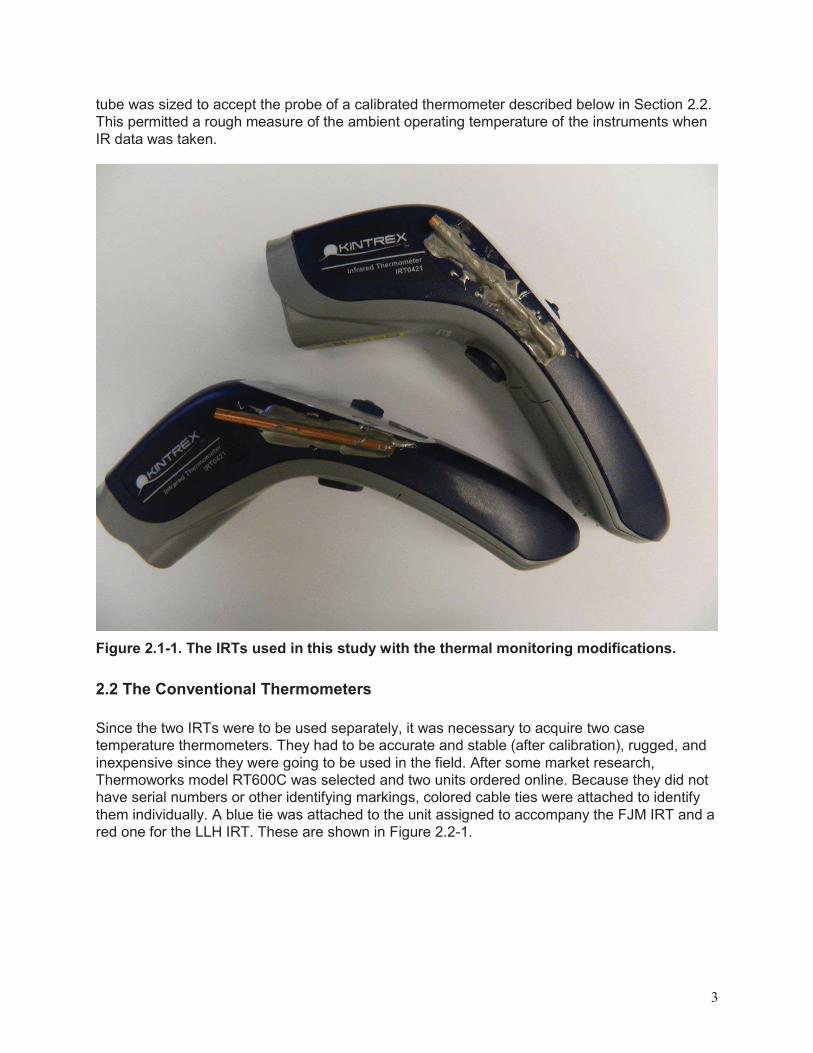
tube was sized to accept the probe of a calibrated thermometer described below in Section 2.2. This permitted a rough measure of the ambient operating temperature of the instruments when IR data was taken.

Figure 2.1-1. The IRTs used in this study with the thermal monitoring modifications.

2.2 The Conventional Thermometers Since the two IRTs were to be used separately, it was necessary to acquire two case temperature thermometers. They had to be accurate and stable (after calibration), rugged, and inexpensive since they were going to be used in the field. After some market research, Thermoworks model RT600C was selected and two units ordered online. Because they did not have serial numbers or other identifying markings, colored cable ties were attached to identify them individually. A blue tie was attached to the unit assigned to accompany the FJM IRT and a red one for the LLH IRT. These are shown in Figure 2.2-1.

4

Figure 2.2-1. The two Thermoworks RT600C thermometers with color-coded identifying cable ties. These instruments cost less than $20 each, have a response time less than six seconds, and are accurate to within 0.5 C over the range -40 to 150 C. Calibrations against our laboratory reference instrument demonstrated that these instruments provided a stable and accurate reference for the case temperatures. Our primary reference instrument for laboratory temperatures was an Oakton Instruments Model Temp5, serial number 878341 with plug-in probe serial number 93X052912 192. It was NIST-traceably calibrated by Innocal with calibration report number 190264. The calibrations were performed at -38.8, 0.0, 50.0 and 120.0 C with deviations from the NIST standard not exceeding 0.2 C. This instrument is shown in Figure 2.2-2.

5

Figure 2.2-2. The Oakton reference standard. Unlike the field thermometers from Thermoworks, the Oakton was an expensive, laboratory-grade instrument which could serve as the primary temperature reference for the project. It has a specified resolution of 0.1 C with an accuracy of 0.2 C from -40 to 125 C.

2.3 Calibration Procedures, Facilities and Fixtures There were several reasons that we undertook a significant amount of calibration work for such a small and informal project rather than simply using the data from the IRTs without additional inquiry. First, we wanted to be able to compare the two units we had purchased to see how much consistency there was between them. That required knowing how much of any difference between them was due to calibration differences as opposed to differences in taking the measurements. Second, we wanted to verify the GCO group’s assertion that ambient temperature measurement was not necessary because of the internal temperature compensation. This required the use of thermometers as described above for measuring the case temperature of each unit, and these two thermometers needed to be calibrated sufficiently that their measurements could be compared reliably. Calibrating IR instruments is difficult because the reference (whether plate or cavity) must have a known emissivity and temperature. The temperature is relatively easy to measure in the laboratory if it is uniform across the reference surface or cavity. The emissivity is not measurable without special capabilities that we do not have, but our Calibration Lab has a

6

suitable device which approximates an emissivity of 1.0 to a sufficient level of accuracy for our purposes as long as the surface does not become contaminated. Unfortunately, even with a dry nitrogen purge, the reference device often developed a layer of dew or frost when the cavity was cooled below the ambient dewpoint, which in Florida was always above 10 C. Scheduling time in the Calibration Laboratory is difficult, and funding was not available for a significant amount of calibration by the lab. In order to collect some additional data under a variety of circumstances, the authors constructed a “mini-cavity” which is described below. It was temperature-controlled in a water bath monitored by the NIST-traceable Oakton thermometer. Like the device used by the Calibration Laboratory, our mini-cavity would rapidly become coated with water when cooled below the dewpoint. The bath was also used to calibrate the Thermoworks case temperature thermometers. Because of the convenience of having faucets and a sink at hand and the risk of spillage when working with a water bath, this work was performed in the Wet Chemistry Lab at KSC. In some cases, calibration measurements were made without the need for running water or significant risk of spillage. These were performed in our office using additional fixtures that are described below. They were primarily related to determining the time constants of the IRTs and attempting to assess their sensitivity to case temperature differences. Finally, sky temperature measurements were made with the instruments operated nearly simultaneously side by side for a direct intercomparison.

2.3.1 The KSC Calibration Laboratory The KSC Calibration Laboratory calibrated both of our Kintrex IRT-0421 units with a Fluke model 9133 Portable Infrared Calibrator. Five test points were used: 5.0, 23.0, 41.0 and 59.0 F (-15.0, -5.0, 5.0, and 15 C). The temperature of the calibrator was monitored using a Fluke model 1502A thermometer readout with an RTD probe. The calibration report (Perry King, private communication) noted that there were difficulties with the test setup and that “even with a high rate of purge there was extensive frost buildup.” The results in that report are shown in Table 2.3.1-1 in the units in which the calibration was performed and reported by the calibration laboratory.

7

Table 2.3.1-1. Calibration Laboratory results for the IRTs.

SN E1032026193 Test Point °F (C)

Indication °F (C)

Error °F (C)

Std Deviation °F (C)

5.0 (-15.0) 10.0 (-12.2) +5.0 (+2.8) ±0.3 (0.2) 23.0 (-5.0) 26.7 (-2.9) +3.7 (+2.1) ±0.4 (0.2) 41.0 (5.0) 43.9 (6.6) +2.9 (+1.6) ±0.0 (0.0) 59.0 (15.0) 59.6 (15.3) +0.6 (+0.3) ±0.2 (0.1)

SN E1032026567 Test Point °F (C)

Indication °F (C)

Error °F (C)

Std Deviation °F (C)

5.0 (-15.0) 9.4 (-12.6) +4.4 (+2.4) ±0.7 (0.4) 23.0 (-5.0) 25.8 (-3.4) +2.8 (+1.6) ±0.4 (0.2) 41.0 (5.0) 43.1 (6.2) +2.1 (+1.2) ±0.3 (0.2) 59.0 (15.0) 59.4 (15.2) +0.4 (+0.2) ±0.1 (0.1) The results in bold italics are outside of the specifications of the Kintrex units, but they are also at temperatures below freezing where frost in the calibration device was a problem. This was one of the motivations for the additional calibration work we performed in the Wet Calibration Laboratory. It should also be noted that the factory calibration of the Kintrex 0421 assumes an emissivity of 0.95 over the range 5 – 14 �m whereas the calibration device is specified to have 0.95 emissivity over the range 8 – 14 �m. It is not known what the emissivity of the calibration device is between 5 and 8 �m, but that may affect the readings. Significantly, the two IRTs showed very similar error characteristics.

2.3.2 The Wet Chemistry Laboratory Early in the planning of the project we realized that we would need to have a method of determining the relative calibrations of our three reference thermometers. It should be available as frequently as needed, cost very little, and be accurate within about 0.1F. Properly executed, an insulated water bath will easily perform that well, so we designed one using readily available off the shelf components.

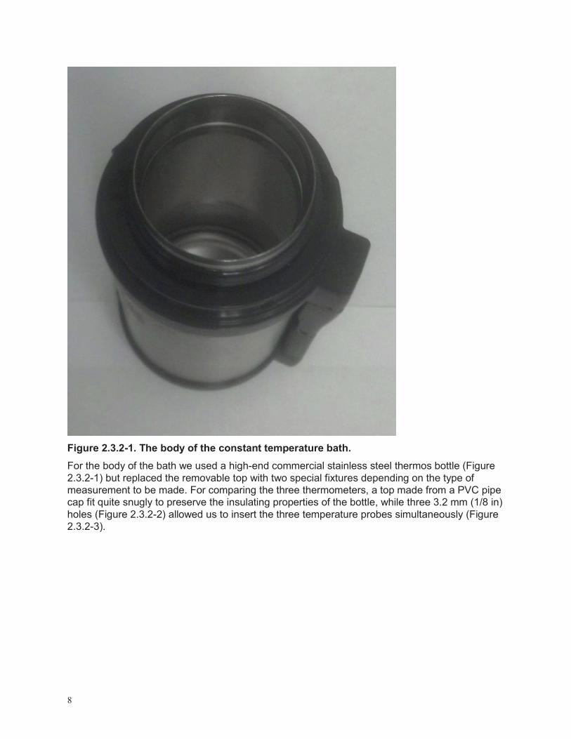
8

Figure 2.3.2-1. The body of the constant temperature bath. For the body of the bath we used a high-end commercial stainless steel thermos bottle (Figure 2.3.2-1) but replaced the removable top with two special fixtures depending on the type of measurement to be made. For comparing the three thermometers, a top made from a PVC pipe cap fit quite snugly to preserve the insulating properties of the bottle, while three 3.2 mm (1/8 in) holes (Figure 2.3.2-2) allowed us to insert the three temperature probes simultaneously (Figure 2.3.2-3).

9

Figure 2.3.2-2. The constant temperature bath cap for thermometer intercomparisons.

Figure 2.3.2-3. The assembled thermometer intercomparison bath. We also wanted to have some way to at least attempt some additional IRT calibrations of our own. We decided to try placing a cylindrical cavity in the constant temperature bath. We epoxied a copper tube 25.4 mm (1 in) diameter by 165 mm (6.5 in) long in the center of another PVC cap and sealed the bottom of the tube with metal and the thermally-conducting epoxy. When the epoxy had hardened, we sprayed the interior surfaces of the tube with Krylon 1602 “ultra flat black” paint which has very high IR emissivity. The completed cavity insert is shown in Figure 2.3.2-4

10

One 3.2 mm hole was drilled for a reference thermometer as shown in Figure 2.3.2-5. In operation, the IRT is aimed straight down the cavity. Its aperture is the same diameter as the tube so its entire field of view should be filled with the cavity and only the cavity.

Figure 2.3.2-4. The IR “mini-cavity” for the constant temperature bath.

11

Figure 2.3.2-5. The IR “mini-cavity” in the constant temperature bath.

2.3.2.1 The Thermoworks thermometers Several tests were performed to evaluate the comparability and time constant of the two Thermoworks thermometers. The first series of tests began with the water in the constant temperature bath cooled below or heated above ambient room temperature. The Thermoworks thermometers were allowed to come to equilibrium at room temperature, then plunged into the bath. After they had come to equilibrium in the bath they were withdrawn and again allowed to come to room temperature equilibrium. The room temperature and bath temperature were both measured with the Oakton reference thermometer. Room temperature ranged from 70.9 to 71.6 F. The bath temperature ranged from 44 to 109 F. The equilibrium temperatures in the bath are shown in Table 2.3.2.1 – 1.

12

Table 2.3.2.1-1. Thermoworks comparison temperatures in the constant temperature bath. Oakton Reference , °F (C)

Red-tagged Thermoworks, °F (C)

Blue-tagged Thermoworks, °F (C)

44.1 (6.7) 44.6 (7.0) 44.4 (6.9) 53.7 (12.1) 53.8 (12.1) 54.2 (12.3) +/- 0.1 (unsteady) 72.1 (22.3) 72.5 (22.5) 72.3 (22.4) 88.1 (31.2) 88.2 (31.2) 88.0 (31.1) 109.4 (43.0) 109.4 (43.0) 109.4 (43.0)

Finally, a relatively crude “ice bath” test was performed by adding crushed ice and distilled water to the constant temperature bath and repeating the same test sequence just described. The resulting reference temperature was 31.9 F (-0.1 C). The red thermometer read 32.4 F (0.2 C) and the blue 32.0 F (0.0 C). When the location of the two Thermoworks thermometers was switched (in case of non-uniformity of the ice bath), the results were 32.5 F (0.3 C) (red) and 32.0 F (0.0 C)(blue). The time constants for the Thermoworks thermometers going from air to water were always between ten and 15 seconds. The time to equilibrium when removed from the bath was more variable but was always less than 240 seconds and sometimes less than 200. Based on these results, it appeared the Thermoworks thermometers could be used as reliable case temperature monitors for the IRTs over the ambient temperature range at which measurements were likely to be made in central Florida. Their response time was fast and their accuracy was within 1C (1.8F) or better in reference to both the Oakton standard and each other.

2.3.2.2 The IRTs The mini-cavity was placed in the constant temperature bath with the red-tagged Thermoworks thermometer as a reference as shown in Figure 2.3.2-5 above. Bath temperatures from 60.3 to 105.1 F (15.7 to 40.6 C) were used. Colder temperatures were not attempted because we had no way of attempting a dry air purge to prevent condensation below the dewpoint which was in the mid-50s F. For the IRTs, the blue-tagged Thermoworks was used to measure the body temperature. Because small differences in the way the IRT was held when the measurement was made could result in slight differences in measured temperatures, four IRT readings were taken at each bath reference temperature for each IRT. Since this took several minutes, the bath temperature and body temperatures were recorded at both the beginning and end of the eight measurement sequence (four measurements for each of two IRTs). The bath temperature, the case temperatures and the IRT measurements were all very stable. In all cases but one, the bath temperature remained constant. In that case, the bath cooled by 0.2 F between the first and last measurement. Case temperatures were, of course, always near room temperature which fluctuated a few tenths of a degree about 71 F (21.7 C). They ranged from 70.5 to 72.3 F (21.4 to 22.4 C) with the largest change during any one set of eight measurements being 1.2 F. The four IRT measurements within any single set for either instrument varied by at most 0.5 F and frequently by only 0.1 F. For that reason, we decided to throw out the highest and lowest of the four readings and average the remaining two to obtain the value for comparison with the reference. The results are presented in Table 2.3.2.2-1.

13

Table 2.3.2.2-1. The IRT Wet Chemistry Lab bath calibration results.

Reference,°F (C) FJM IRT,°F (C) LLH IRT,°F (C) 105.1 (40.6) 106.9 (41.6) 106.3 (41.3) 96.8 (36.0) 97.9 (36.6) 97.8 (36.6) 87.0 (30.6) 87.3 (30.7) 87.0 (30.6) 77.0 (25.0) 76.5 (24.7) 76.9 (24.9) 69.8 (21.0) 68.9 (20.5) 69.1 (20.6) 60.3 (15.7) 58.7 (14.8) 58.9 (14.9) The results are very good at or near room temperature. These measurements are combined with additional measurements made in the office in section 2.3.3.4 below.

2.3.3 Office calibrations There was another option for some of the instrument characterization and calibration tests we wanted to do which did not require access to water. It was more convenient to do these in our normal office environment. We needed a competent IR target with high emissivity and large thermal inertia so that its time constant was significantly longer than the time it takes to make a measurement, and a way of heating of cooling either the target, the IRTs, or both. For the target, we purchased a 305 cm (12 in) square aluminum plate 0.63 cm (1/4 in) thick and had three holes 0.32 cm (1/8 in) x 15.3 cm (6 in) deep drilled in one edge for insertion of one or more reference thermometers. The surface was painted with the same high emissivity paint used for the mini-cavity discussed above. The plate appears as part of Figure 2.3.3-1 which is discussed below. For cold-soaking or hot-soaking the plate or the IRTs, we used two ice chests and hot water bottles or bags of ice. Small holes were placed in the lids of the ice chests for reference thermometers. An IRT or the plate could be placed in an ice chest with hot water bottles or bagged ice and the chest allowed to come to equilibrium as indicated by the inserted thermometer. Then the instrument or plate could be removed for use as described later in this section.

14

Figure 2.3.3-1. IR calibration fixture made from an ice chest and the calibration plate. Near the end of the project, one of the ice chests was modified to make a dedicated IR calibration box by cutting slots in two sides to allow the plate to be inserted at an angle with the box sealed except for holes in the lid to insert the thermometers in the plate and a port in a third side through which the IRT would view the plate as shown in Figure 2.3.3-1.This allowed the use of ice bags to create a stable temperature reference for intercomparing the two IRTs essentially simultaneously against the same reference at cooler temperatures than we could obtain without this fixture. We could observe whether there was any dew or frost on the surface of the plate, but it was never cooled enough for that to occur.

2.3.3.1 The time constant of the IR target plate The time constant of the aluminum plate to be used as a target for IRT comparisons and calibrations was determined by heating it above ambient temperature in one of the ice chests with a hot water bottle and then monitoring its temperature as it returned to ambient when removed from the chest. The plate was enclosed in an unsealed plastic bag to protect it from any possible leak in the hot water bottle. The ice chest was closed for at least an hour. Its internal air temperature was monitored with one of the Thermoworks thermometers to ensure that the enclosure had reached a stable temperature at least 10 F above ambient. After the temperature in the enclosure had stabilized and at least an hour had passed, the plate was removed from the plastic bag and set with its bottom on the rug and its top resting against

15

the ice chest with both the front (IR-blackened) and rear (polished aluminum) faces fully exposed to the ambient air. The red-tagged Thermoworks thermometer was inserted into the center thermometer hole in the plate and temperatures recorded at roughly one minute intervals for the first ten minutes, and then at increasingly longer intervals as the rate of change of temperature declined. After 6 minutes had elapsed, one of the IRTs was used to examine all four corners, the top and bottom edges and the center of the plate to determine how uniform the temperature was across the plate. The measurements always were within 0.2 F when comparing any two points on the plate within 15 seconds or so. The results are shown in Figure 2.3.3.1-1. The time constant calculated from the exponential least squares fit was 20.8 minutes.

Figure 2.3.3.1-1. IRT calibration plate time constant measurements.

2.3.3.2 The time constant of the IRT instrument cases The process described immediately above for determining the time constant of the calibration plate was also used to determine the time constant of the IRT case temperatures. The two IRTs were processed separately. The red-tagged thermometer was used with the FJM IRT and the blue one with the LLH IRT. The thermometers were inserted into the copper tube affixed to the IRT case as soon as the IRT was removed from the ice chest. The IRT with its thermometer was laid on top of the closed ice chest. This exposed all but one side to the ambient air. The top of the ice chest is insulating Styrofoam, which was at or very near the ambient room temperature. Because the two IRTs were tested separately, their starting temperatures were not the same, but as shown in Figure 2.3.3.2-1, they had essentially identical slopes to the exponential least squares fit, equivalent to a time constant of about 28 minutes.

16

Figure 2.3.3.2-1. The IRT temperature time constant measurements.

2.3.3.3 The sensitivity of the IRTs to changes in case temperature Our attempts to confirm that the internal temperature compensation circuitry in the IRTs worked acceptably were limited. The reference plate was allowed to come to room temperature equilibrium with the red Thermoworks thermometer in the center thermometer port. The case temperature of the IRTs was measured with the blue Thermoworks after the IRT has been allowed to come to equilibrium in one of the ice chests with a hot water bottle. Unfortunately, this methodology could only produce case temperatures less than 11 F above ambient because of the limited heat capacity of the hot water bottle. We were reluctant to try cooling the IRTs in the ice chest because of the possibility that we could cause condensation to form inside the units and thereby damage them. The results of these limited explorations are shown in Figure 2.3.3.3-1.

17

Figure 2.3.3.3-1. IR and case temperature differences from ambient. In our judgment, these results are inconclusive for several reasons. First, even taken at face value, the data show a negative slope for case temperatures near ambient, a positive slope for temperatures 4 to 8 degrees above ambient, and no temperature sensitivity from 8 to 11 degrees above ambient, which provides no reliable indication of any real, consistent sensitivity given the small range and sample size. Second, the data cannot be taken at face value, because we noted what we called a “hand effect” when taking data. Specifically, the case temperature appeared to elevate by several tenths of a degree F when a reading was being taken. We strongly suspect that the heat from our hand as we held the IRT slightly warmed the copper tube in which the Thermoworks thermometer was placed. This effect differed in magnitude depending on the case temperature. We had tentatively planned to attempt measurements with case temperatures below ambient at the end of the project when damage to the IRTs would be least disruptive to the project. After examining the field measurements and especially the results presented in section 2.3.4.2 below we felt confident enough that the internal compensation was effective to abandon any additional efforts in the lab or office.

2.3.3.4 Office calibrations and intercomparisons of the two IRTs In addition to the simultaneous calibrations of the two instruments described above in section 2.3.2.2 above, we performed a number of measurements using the target plate in an office environment. These included ambient temperature measurements where the plate and both IRTs were allowed to come to equilibrium with the room temperature, and measurements made

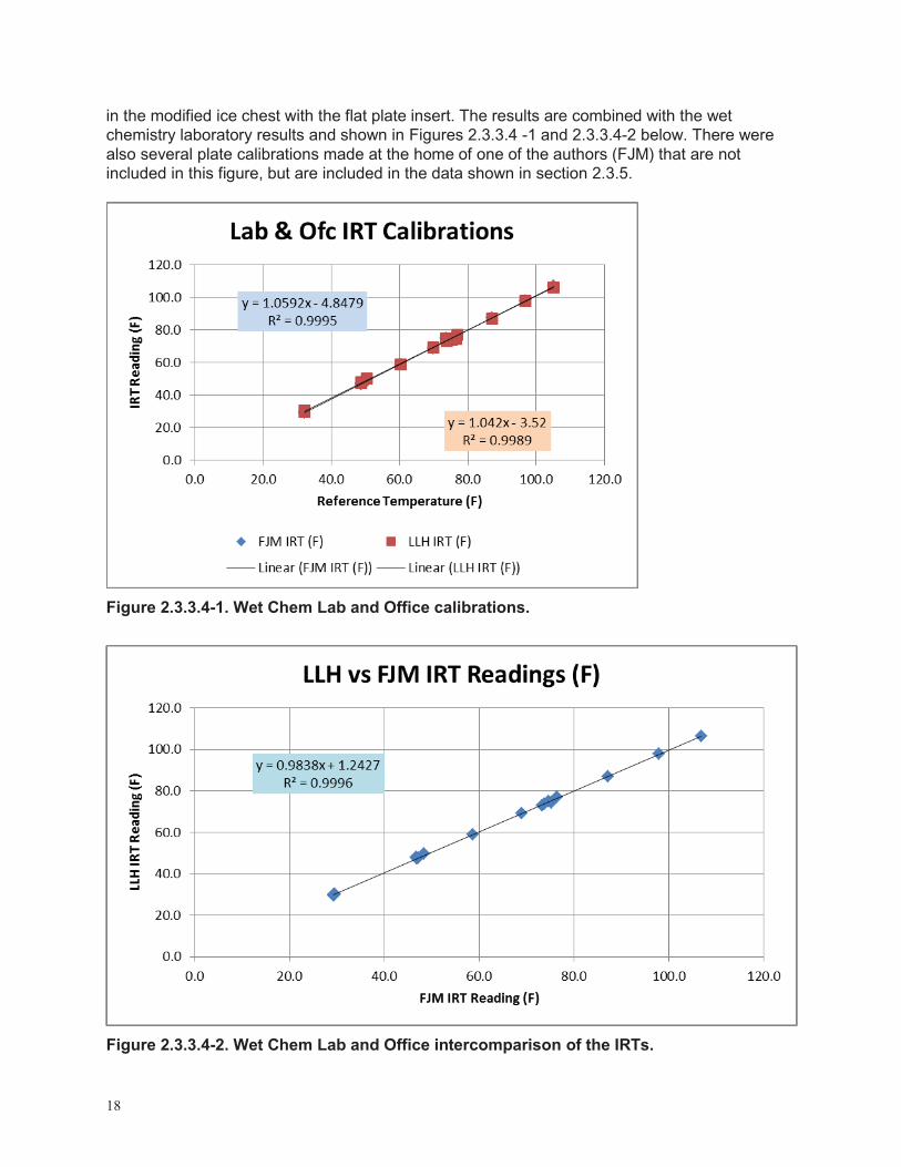
18

in the modified ice chest with the flat plate insert. The results are combined with the wet chemistry laboratory results and shown in Figures 2.3.3.4 -1 and 2.3.3.4-2 below. There were also several plate calibrations made at the home of one of the authors (FJM) that are not included in this figure, but are included in the data shown in section 2.3.5.

Figure 2.3.3.4-1. Wet Chem Lab and Office calibrations.

Figure 2.3.3.4-2. Wet Chem Lab and Office intercomparison of the IRTs.

19

2.3.4 Field calibration of the two IRTs In addition to calibration in laboratory and office environments, additional assessments of the performance characteristics of the IRT instruments were made using the indicated sky temperature measurements. Measurements from the two instruments at or near the same time and place were compared to provide an estimate of measurement uncertainty. An assessment of the effects, if any, of case temperature on the measured sky temperature was also attempted.

2.3.4.1 Field intercomparisons of the two IRTs In thirteen cases, we made simultaneous indicated sky temperature measurements with the two IRTs at the same location, and we had one additional case where the two measurements were nearly simultaneous but from locations separated by about 10 km. The agreement is very good as shown in Figure 2.3.4.1-1.

Figure 2.3.4.1-1. IRT indicated sky temperature intercomparisons.

2.3.4.2 Temperature sensitivity Because the laboratory examination of the effects of case temperature were inconclusive as described in section 2.3.3.3, we used the field measurements to provide some additional assessment of this concern. In 60 cases where we had case temperatures and valid sky temperature measurements, we made at least two measurements within a few minutes from the

20

same location. Specifically, we had 20 sets of two measurements, 33 sets of three, 5 sets of four and one each of six and nine measurements within 10 minutes or less. For each of those cases we averaged both the case temperature readings and the IRT readings and computed the differences from the average for each of the separate measurements within the average. The departure of the IRT reading from the mean is plotted against the departure of the case temperature in Figure 2.3.4.2-1.

Figure 2.3.4.2-1. IR vs. case temperature departures from the mean. The sky temperature is assumed to be constant during the period because even with the relatively small field of view of the IRTs, the volume of atmosphere sampled is quite large and unlikely to have significant rapid changes in IPW. The scatter in the IR reading is assumed to represent random sampling error plus the effect, if any, of changes in the case temperature. The case temperature can vary for a variety of reasons including but not limited to the conduction from the atmosphere or the hand holding the instrument, internal heating due to activation of the instrument, or inadequate time allowed for the instrument to reach equilibrium with the environment. The figure shows that the IRT departures are completely uncorrelated with the case temperature departures. This is consistent with the assertion in BAMS that the internal thermal correction is effective.

2.3.5 Overall Calibration of the IRTs As noted earlier in this report, there were several different sources of calibration data for the IRTs. These include the Calibration laboratory data, the Wet Chemistry Laboratory data,

21

comparisons in the office and plate calibrations at the home of an author. When combined, these show a consistent level of reliability and accuracy that is quite gratifying given the informal and sometimes crude methodologies used and the inexpensive consumer-grade instrumentation being calibrated. The complete calibrations for the ITRs are shown in Figures 2.3.5-1 and 2.3.5-2.

Figure 2.3.5-1. Combined calibrations of the FJM IRT.

22

Figure 2.3.5-2. Combined calibrations of the LLH IRT. If these same data are used to compare the LLH IRT against the FJM IRT for mutual consistency, we obtain the result shown in Figure 2.3.5-3.

23

Figure 2.3.5-3. The LLH IRT readings as a function of the FJM IRT readings during calibrations. If the sky temperature comparisons are added to the data in Figure 2.3.5-3 we have the overall composite of all of the comparison data as shown in Figure 2.3.5 -4

24

Figure 2.3.5-4. The LLH IRT readings as a function of the FJM IRT readings for all comparisons. Although the parameters of the linear least squares regressions are slightly different, the overall difference between the two instruments appears to be on the order of one degree F or less over the entire range from near -20 F to over 100 F. This is of the same order of the scatter in the measurements and indicates that for practical purposes, the two instruments may be treated as identical.

2.4 Field Data Collection This section describes the methodology for acquiring the GPS and balloon reference integrated precipitable water data and for taking the IRT sky measurements. The IRT sky readings will be referred to as “indicated sky temperatures” because the IR thermometer calculates a “temperature” assuming it is looking at a surface with black body characteristics and an emissivity of 0.95. The sky is not a surface nor is it a black body. The measurement by the zenith-directed IRT is of radiation emitted by a volume rather than a surface and any “temperature” varies within that volume. In the spectral region of interest, the emissivity for water vapor, in particular, varies significantly with wavelength (Petty, 2006). For that reason, the temperature indicated by the IRT cannot really be said to be the temperature of anything specific: it is just the temperature “indicated” by the device.

25

2.4.1 GPS and Sounding Data Used as “Ground Truth” NOAA’s CCV6 GPS IPW site located on Cape Canaveral Air Force Station near 28.46N, 80.55W and soundings from the CCAFS balloon facility (ID = XMR) near 28.48N, 80.56W were used as the data against which regressions of IRT sky temperatures were generated. Sounding data was only available once or twice daily, but GPS data was usually available every 30 minutes. When the GPS data was available, the GPS IPW reading closest in time to each sky temperature reading was used as the “ground truth” reference for that reading. If timely GPS data was not available, the nearest XMR sounding in time was used instead. Although the agreement between the soundings and the GPS data was generally excellent, there was a period during the early summer of 2013 where the soundings often appeared to be drier than either the GPS or nearby soundings. It is believed that there was a possible defect in the batch of sondes used at XMR to make those measurements, and during that period, sounding data was ignored.

2.4.2 IRT Data IRT measurements were made at five sites as shown in Table 2.4.2-1.

Table 2.4.2-1. Locations at which sky temperatures were taken. Description N. Latitude W. Longitude CCV6 distance (km) KSC Headquarters Building 28.52 80.65 12.6 KSC Operations Support Building I 28.58 80.65 17.4 Morrell Operations Center 28.43 80.59 6.3 Author’s Home (FJM) 28.45 80.71 15.8 Author’s Home (LLH) 28.40 80.75 21 AMU PM’s Home 28.20 80.71 32.9

Mims et al. (2011) used sun photometers as their primary reference because they found they correlated better with the sky temperatures than GPS readings. They speculated that this may have resulted from the fact that their sun photometers were essentially co-located with the IRT measurements whereas their GPS measurements were more than 30 km away from the IRT measurement site. Most of our comparisons involved separation distances of half that or less as shown in Table 2.4.2-1. We followed the protocol from Mims et al. (2011) for taking field measurements. It can be difficult to know if the IRTs were truly pointed to zenith. To compensate for this difficulty we made multiple measurements at the same time and place. We then recorded the lowest temperature observed based on the assumption that the straightest path to zenith would give the lowest temperature. We made measurements during most hours of the day except for the period from 11 PM through 4 AM EST as shown in Figure 2.4.2-1. In the figure, as in our data set, the time is recorded in UTC. EST is equal to UTC – 5 hours. Our local solar time is approximately EST – 20 minutes.

26

Figure 2.4.2-1. Sample size as a function of hour of day (UTC). The times of sunrise and sunset vary throughout the year but sunrise is always within about an hour of 11 UTC and sunset roughly within an hour of 23 UTC. As the figure shows, our observations were biased towards the hours just after sunrise and just before sunset. The local noon hour was deliberately avoided because the sun would be too close to the zenith and might get into the field of view of the instrument. Otherwise, we tended to make our measurements in the morning before or just after arriving at work or in the evening before or just after leaving the office for the day. Table 2.4.2-2 shows the sample size distribution I categorical form.

Table 2.4.2-2. Sample size as a function of segment of day. Segment of Day Count Percent Night 17 7.7 Near Sunrise 37 16.8 Daytime 104 47.3 Near Sunset 62 28.2 Total 220 100

If the zenith sky is cloudy, then the IRT essentially measures the cloud base temperature rather than the IPW, so it was important to note the sky conditions when making observations. We printed prepared forms using a spreadsheet which contained fields for the date, time and location of each observation, the case temperature, the sky temperature, and notes on the sky condition and anything else that might affect the representativeness of the reading. This served the dual purpose of reminding us of the need to pay attention to the sky conditions before committing to a measurement and to document that we had done so.

27

Chapter 3. Results

3.0 Overview As noted in Chapter 1, the reference data for evaluating the performance of the IRTs as IPW instruments was to be measured by comparison with nearby NOAA GPS IPW data and soundings from Cape Canaveral Air Force Station. The GPS IPW data are available at 15 and 45 minutes past the hour UTC from NOAA site CCV6 through the NOAA GPS data access gateway at http://gpsmet.noaa.gov/cgi-bin/gnuplots/rti.cgi. The sounding data are available for 11:15 UTC for CCAFS (XMRB) and are also available on the NOAA GPS website. Unless it was unavailable or suspect, we used the GPS IPW observation closest in time to each IRT measurement as the reference value for that measurement. In some cases, the GPS data were not available. In those cases if there was a sounding less than four hours from the time the IRT data were collected, it was used as the reference. We compared the soundings with the GPS data when both were available in order to assure that the two data sources were comparable. The simple bias between the two data sources is -0.032 and the mean average error (MAE) is 0.186. The results presented in Figure 3.0-1 demonstrate that the soundings and the GPS are mutually consistent data sources. In the discussions that follow, where no distinction is made between the GPS and sounding data it is referred to as the “composite” IPW.

28

Figure 3.0-1. GPS IPW vs. Sounding IPW. Based on the calibration results in section 2.3.5 above showing that the two IRT instruments could be treated as identical for practical purposes, we sometimes combined the sky temperature measurements from the two instruments into a single composite sky temperature database called “KSCIR” to increase the sample size over what was available from the FJM and LLH instruments separately.

3.1 Sky temperature regressions against GPS/sounding IPW All of the IRT sky temperature measurements collected with both IRTs are plotted in Figure 3.1-1.

29

Figure 3.1-1. The separate IRT measurements vs. composite IPW. The data are fitted to a logarithmic curve which is equivalent to the exponential fits used by Mims et al. with the dependent and independent variables reversed. Note that the difference between the two IRTs is everywhere within the scatter of the measurements. The results when the data are combined are presented in Figure 3.1-2.

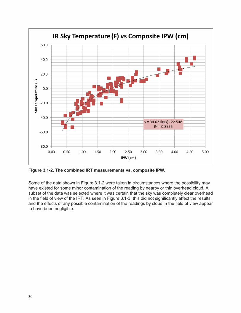
30

Figure 3.1-2. The combined IRT measurements vs. composite IPW. Some of the data shown in Figure 3.1-2 were taken in circumstances where the possibility may have existed for some minor contamination of the reading by nearby or thin overhead cloud. A subset of the data was selected where it was certain that the sky was completely clear overhead in the field of view of the IRT. As seen in Figure 3.1-3, this did not significantly affect the results, and the effects of any possible contamination of the readings by cloud in the field of view appear to have been negligible.

31

Figure 3.1-3. The combined clear sky IRT measurements vs. composite IPW.

3.2 Comparison of our regressions with those of the GCO team In addition to determining that there was a dependable relationship between the IR sky temperature and IPW, we also wanted to see how closely that relationship agreed with the relationship reported by the GCO team. Since the relationship depends on the field of view and spectral response of the IRT, we compared our results only with the GCO results for the Kintrex 0421. In Mims et al. (2011), Figure 7, the following equation is given: y = -0.141 + 3.333*exp(-x/-29.851) (3.2-1) where y is the IPW (cm) measured by the Microtops instrument described in the article and x is the zenith sky temperature measured by the IRT0412 (C). This equation may be inverted to give the equivalent GCO IRT reading as a function of IPW since the relationship between them is

32

monotonic. The initial intention was simply to plot the computed GCOIR along with the KSCIR as a function of IPW and see how they compare. It turned out to be more complicated than that. Figure 3.2-1 shows the comparison of the computed GCO IR temperatures computed from equation 3.2-1 with the measured KSC IR temperatures for the same values of IPW. The data is a subset of all of the data obtained by eliminating balloon data and eliminating essentially redundant data. As previously noted in section 2.3.4.2 above, at any given time we usually took multiple measurements. These were not independent. In the figures in this section, each of those near-simultaneous sets of measurements has been replaced by the average of all of the values in the set.

Figure 3.2-1. KSC and GCO indicated sky temperatures vs. IPW. While the general shapes of the curves are the same, the agreement is not as good as we had hoped, and the difference between the two curves clearly exceeds the scatter in the measurements. A more careful analysis indicated why. There is a critical adjustment that needed to be made to the GCO equation in order for the results to be comparable with ours. Our IPW reference was GPS, but the GCO reference for equation 3.2-1 is a sun photometer called “MICROTOPS II”. It does not give the same values for IPW as the GPS does. To cross calibrate the MICROTOPS II with GPS, we used Mims et al. Figures 3 and 4 which compared a different IRT (an Omega OS540) with the MICROTOPS II and GPS respectively. The equivalent figures were not available for the Kintrex units, but we are

33

willing to assume that the OS540 response is sufficiently similar to permit it to be used as a transfer standard for determining the relation between the GPS and the sun photometer for our use. Combining the data from the two figures, we generated a regression between the difference in sky temperatures using GPS and MICROTOPS for a given GPS value of the IPW. The result was a second order polynomial that fit the data perfectly as shown in Figure 3.2-2

Figure 3.2-2. Difference in indicated sky temperatures between GPS and Sun Photometer reference instruments for give GPS IPW. When this adjustment is applied to the GCO computed values, the result is significantly closer to ours and within the scatter of the measurements as shown in Figure 3.2-3. The remaining differences may include not only the effects of sampling error and natural variance, but also the effects of local site variations that are not adequately captured in the GPS retrieval algorithms (Bevis et al., 1992). One such local variation that is likely is azimuthal anisotropy in low level atmospheric moisture due to the coastal location of the GPS site. Azimuthal isotropy is assumed in the GPS IPW calculation (Wolfe and Gutman, 2000; Bevis et al., 1992) and violation of that assumption can lead to errors in the results (ibid). Since the effects of this anisotropy are almost certainly dependent on the mean wind direction and vertical profiles of water vapor onshore and off shore, it probably increases the scatter in our data as these properties may differ for any given IPW value.

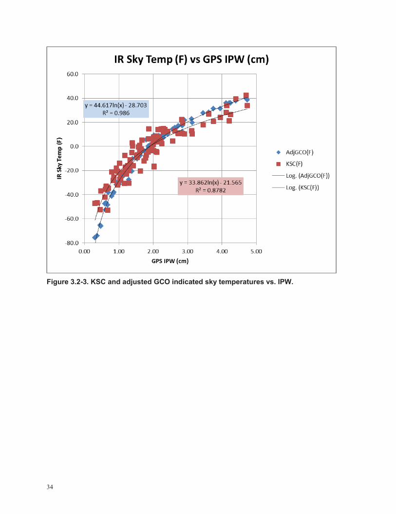
34

Figure 3.2-3. KSC and adjusted GCO indicated sky temperatures vs. IPW.

35

Chapter 4. Summary, Discussion and Conclusion

4.0 Summary We have demonstrated that the use of inexpensive commercial off the shelf handheld infrared thermometers to estimate IPW from IR sky temperature measurements as suggested by Mims et al . (2011) can be replicated in our sub-tropical environment. The instruments as delivered from the vendor gave consistent, repeatable results without special adjustment, tuning or handling. Our results were quantitatively within the scatter of the data of those of the GCO team (ibid) even though their instrument and ours were purchased from separate sources several years apart and operated in different natural environments that could contribute some site-specific variations to the GPS measurements against which they were compared.

4.1 Discussion The IRT instruments cost less than $50 (latest on-line price at the time this is being written) and they are extremely portable. GPS IPW stations cost between 10 and 20 thousand dollars per receiver/antenna a decade ago (Wolfe and Gutman, 2000) and are still cost prohibitive for high-density applications. Radiosonde systems can’t be carried in your briefcase and costs for radiosonde measurements will vary with the amount of flight elements needed (~$250 to $500 per flight not including ground equipment costs.) Satellite observations may not be available when or where they are needed. The IRT sky temperature measurement technique opens the door to IPW measurements when and where there are needed at extremely low cost. There are, of course, limitations. While most of the standard methods work under a wide range of ambient weather conditions, the IRT method requires clear sky near the zenith. This can be an extremely restrictive constraint, especially in some climates during some seasons. Nonetheless, the effectiveness of the IRT method poses some very interesting opportunities. One of the areas of ongoing research where these instruments may be of assistance is improving our understanding of the spatial and temporal scales of IPW variability, especially where influences from mountains or coastlines may be important. Most GPS measurements lack the density and resolution to characterize mesoscale fluctuations in IPW which may reach 0.5 cm or more in less than 20 km (see, e.g., Bastin et al., 2007, Figure 6). The power spectrum of IPW fluctuations is continuous and has been observed to have characteristics similar to wind and temperature fluctuations in the mesoscale range (Zhu et al., 2008). One way of approaching this would be through the use of structure functions (see, e.g., Haase et al., 2003). The key to observing these small scale features and being able to compute spatial structure functions or spectra is the ability to make many measurements with horizontal spacing close enough to resolve the scales of interest. We envision the possibility of a university or other research program acquiring dozens of these IRTs and hiring students or others to operate them at selected locations during intensive observing intervals. Even including the cost of hourly labor, a line of 20 or more optimally spaced measurements could be made for a small fraction of the cost of obtaining similar resolution in space and time from conventional measurements.

36

Another application we envision is for campers, hikers, prospectors, hunters or others who spend significant time in areas with low population density and no convenient access to local weather data beyond what they can see for themselves. Hanssen et al. (1999) noted the utility of high resolution IPW for forecasting the local onset of storms. An IRT instrument can provide individuals with a personal sensor for detecting changes in the state of the atmosphere that might not otherwise obviously manifest themselves. We once observed a 20 degree F drop in the sky temperature between two readings taken about three hours apart. When the second reading was taken, we initially suspected that we had incorrectly recorded the first reading. When we obtained the GPS data for the period we saw that over the three hours between the two IRT readings, the IPW had dropped from about 1.2 cm to less than 0.7 mm as shown in Figure 4.1-1. A subsequent examination of synoptic surface data showed that some sort of dry boundary not otherwise accompanied by significant weather had passed over us during the time between the readings. Such a feature could be important to severe weather warnings under different weather conditions.

Figure 4.1-1. GPS IPW and KSC IRT indicated sky temperatures for 23 November 2012.

4.2 Conclusion This limited and somewhat informal investigation has replicated the methodology presented in Mims et al. (2011) and demonstrated its general utility. The inexpensive, portable nature of the hand-held IR thermometers opens a variety of interesting opportunities for both operations and research related to integrated precipitable water. Small networks of these hand-held IR thermometers could be used to augment GPS-IPW, RAOBs, and satellite-derived IPW for a variety of tasks. For example, they could be used in the vicinity of incident/emergency sites to enhance high resolution local weather modeling or by students and scientists to monitor longer term water vapor trends in climate studies. They could

37

even be used by military personnel in the field where GPS, RAOBs, and satellite coverage is sparse.

38

References

Bastin, S., C. Champollion, O. Block, P. Drobinski, and F. Masson , 2007: Diurnal Cycle of Water Vapor as Documented by a Dense GPS Network in a Coastal Area during ESCOMPTE IOP2, J. Appl. Meteor. Clim. 46,167 – 182. Bevis, M, S. Businger, T.A. Herring, C. Rocken, R.A. Anthes and R.H. Ware, 1992: GPS Meteorology: Remote Sensing of Atmospheric Water Vapor Using the Global Positioning System, J. Geophys Res., 97, 15787-15801. Haase, J., M. Ge, H. Vedel, and E. Calais, 2003: Accuracy and Variability of GPS Tropospheric Delay Measurements of Water Vapor in the Western Mediterranean, J. Appl. Meteor.,42, 1547 – 1568. Hanssen, R.F., T.M. Weckworth, H.A. Zebker and R. Klees, 1999: High Resolution Water Vapor Mapping from Interferometric Radar Measurements, Science,283, 1297 – 1299. Kehrer, K., B. Graf, and W. P. Roeder, 2008: Global Positioning System (GPS) Precipitable Water in Forecasting Lightning at Spaceport Canaveral, Weather And Forecasting, Vol. 23, No. 2, Apr 08, 219-232 Mazany, R., S. Businger, S. I. Gutman, and W. P. Roeder, 2002: A Lightning Prediction Index That Utilizes GPS Integrated Precipitable Water Vapor, Weather and Forecasting, 17, 1034-1047 Mims, Forrest M., L.H. Champers, and D.R. Brooks, 2011: Measuring total column water vapor by pointing an infrared thermometer at the sky, Bull. Am. Met. Soc., 92, 1311 – 1320. Petty, G.G., 2006: A First Course in Atmospheric Radiation, 2d. Edition, Sundog Publishing, Madison, WI, 459 pp. Roeder, W. P., K. Kehrer, and B. Graf, 2010: Using Timelines Of GPS-measured Precipitable Water in Forecasting Lightning at Cape Canaveral AFS and Kennedy Space Center, 3rd International Lightning Meteorology Conference, 21-22 Apr 10, 8 pp. Wolfe, D.E. and S.I. Gutman, 2000: Developing an Operational, Surface-Based, GPS, Water Vapor Observing System for NOAA: Network Design and Results, J. Atm. Ocean. Tech., 17, 426 – 440. Zhu, M., G. Wadge, R.J. Holley, I.N. James, P.A. Clark, C. Wang and M.J. Woodage, 2008: Structure of the precipitable water field over Mount Etna, Tellus, 60A, 679-687.

REPORT DOCUMENTATION PAGE

Standard Form 298 (Rev. 8/98) Prescribed by ANSI Std. Z39.18

Form Approved OMB No. 0704-0188

The public reporting burden for this collection of information is estimated to average 1 hour per response, including the time for reviewing instructions, searching existing data sources, gathering and maintaining the data needed, and completing and reviewing the collection of information. Send comments regarding this burden estimate or any other aspect of this collection of information, including suggestions for reducing the burden, to Department of Defense, Washington Headquarters Services, Directorate for Information Operations and Reports (0704-0188), 1215 Jefferson Davis Highway, Suite 1204, Arlington, VA 22202-4302. Respondents should be aware that notwithstanding any other provision of law, no person shall be subject to any penalty for failing to comply with a collection of information if it does not display a currently valid OMB control number. PLEASE DO NOT RETURN YOUR FORM TO THE ABOVE ADDRESS.

1. REPORT DATE (DD-MM-YYYY) 2. REPORT TYPE 3. DATES COVERED (From - To)

4. TITLE AND SUBTITLE 5a. CONTRACT NUMBER

5b. GRANT NUMBER

5c. PROGRAM ELEMENT NUMBER

5d. PROJECT NUMBER

5e. TASK NUMBER

5f. WORK UNIT NUMBER

6. AUTHOR(S)

7. PERFORMING ORGANIZATION NAME(S) AND ADDRESS(ES) 8. PERFORMING ORGANIZATION REPORT NUMBER

10. SPONSOR/MONITOR'S ACRONYM(S)

11. SPONSOR/MONITOR'S REPORT NUMBER(S)

9. SPONSORING/MONITORING AGENCY NAME(S) AND ADDRESS(ES)

12. DISTRIBUTION/AVAILABILITY STATEMENT

13. SUPPLEMENTARY NOTES

14. ABSTRACT

15. SUBJECT TERMS

16. SECURITY CLASSIFICATION OF:a. REPORT b. ABSTRACT c. THIS PAGE

17. LIMITATION OF ABSTRACT

18. NUMBER OF PAGES

19a. NAME OF RESPONSIBLE PERSON

19b. TELEPHONE NUMBER (Include area code)

06/30/2014 Final Jan 2012 - Jun 2014

Assessment of a Technique for Estimating Total Column Water Vapor Using Measurements of the Infrared Sky Temperature

Francis J. Merceret Lisa L. Huddleston

Kennedy Space Center Weather Office Mail Code: GP-B Kennedy Space Center, FL 32899

NASA/TM-2014-218368

Unclassified, Unlimited

A method for estimating the integrated precipitable water (IPW) content of the atmosphere using measurements of indicated infrared zenith sky temperature was validated over east-central Florida. The method uses inexpensive, commercial off the shelf, hand-held infrared thermometers (IRT). Two such IRTs were obtained from a commercial vendor, calibrated against several laboratory reference sources at KSC, and used to make IR zenith sky temperature measurements in the vicinity of KSC and Cape Canaveral Air Force Station (CCAFS). The calibration and comparison data showed that these inexpensive IRTs provided reliable, stable IR temperature measurements that were well correlated with the NOAA IPW observations.

weather, meteorology, hand held infrared temperature (IRT) measurement, infrared (IR) zenith sky temperature, integrated precipitable water (IPW), east central Florida, Kennedy Space Center, Cape Canaveral Air Force Station

U UU UU UU 50

Lisa L. Huddleston

(321) 861-4952