assessment of crop yield losses in punjab and haryana using 2

Atmos. Chem. Phys., 15, 9555–9576, 2015

www.atmos-chem-phys.net/15/9555/2015/

doi:10.5194/acp-15-9555-2015

© Author(s) 2015. CC Attribution 3.0 License.

Assessment of crop yield losses in Punjab and Haryana

using 2 years of continuous in situ ozone measurements

B. Sinha1, K. Singh Sangwan1,2, Y. Maurya1, V. Kumar1, C. Sarkar1, B. P. Chandra1, and V. Sinha1

1Department of Earth and Environmental Sciences, Indian Institute of Science Education and Research Mohali, Sector 81,

S. A. S Nagar, Manauli PO, Punjab, 140306, India2Department of Geology, Centre of Advanced Studies, University of Delhi, Delhi, 110007, India

Correspondence to: B. Sinha ([email protected])

Received: 8 October 2014 – Published in Atmos. Chem. Phys. Discuss.: 23 January 2015

Revised: 31 July 2015 – Accepted: 3 August 2015 – Published: 27 August 2015

Abstract. In this study we use a high-quality data set of in

situ ozone measurements at a suburban site called Mohali

in the state of Punjab to estimate ozone-related crop yield

losses for wheat, rice, cotton and maize for Punjab and the

neighbouring state Haryana for the years 2011–2013. We in-

tercompare crop yield loss estimates according to different

exposure metrics, such as AOT40 (accumulated ozone expo-

sure over a threshold of 40) and M7 (mean 7-hour ozone mix-

ing ratio from 09:00 to 15:59), for the two major crop grow-

ing seasons of kharif (June–October) and rabi (November–

April) and establish a new crop-yield–exposure relationship

for southern Asian wheat, maize and rice cultivars. These

are a factor of 2 more sensitive to ozone-induced crop yield

losses compared to their European and American counter-

parts.

Relative yield losses based on the AOT40 metrics ranged

from 27 to 41 % for wheat, 21 to 26 % for rice, 3 to 5 %

for maize and 47 to 58 % for cotton. Crop production losses

for wheat amounted to 20.8± 10.4 million t in the fiscal year

of 2012–2013 and 10.3± 4.7 million t in the fiscal year of

2013–2014 for Punjab and Haryana taken together. Crop pro-

duction losses for rice totalled 5.4± 1.2 million t in the fiscal

year of 2012–2013 and 3.2± 0.8 million t in the year 2013–

2014 for Punjab and Haryana taken together. The Indian Na-

tional Food Security Ordinance entitles ∼ 820 million of In-

dia’s poor to purchase about 60 kg of rice or wheat per person

annually at subsidized rates. The scheme requires 27.6 Mt of

wheat and 33.6 Mt of rice per year. The mitigation of ozone-

related crop production losses in Punjab and Haryana alone

could provide > 50 % of the wheat and ∼ 10 % of the rice

required for the scheme.

The total economic cost losses in Punjab and Haryana

amounted to USD 6.5± 2.2 billion in the fiscal year of 2012–

2013 and USD 3.7± 1.2 billion in the fiscal year of 2013–

2014. This economic loss estimate represents a very conser-

vative lower limit based on the minimum support price of the

crop, which is lower than the actual production costs. The

upper limit for ozone-related crop yield losses in all of India

currently amounts to 3.5–20 % of India’s GDP.

The mitigation of high surface ozone would require rela-

tively little investment in comparison to the economic losses

incurred presently. Therefore, ozone mitigation can yield

massive benefits in terms of ensuring food security and

boosting the economy. The co-benefits of ozone mitigation

also include a decrease in the ozone-related mortality and

morbidity and a reduction of the ozone-induced warming in

the lower troposphere.

1 Introduction

India is a rapidly developing nation. Population growth, ur-

banization and industrial development have led to increasing

emissions and have resulted in a statistically significant in-

crease in the tropospheric ozone mixing ratios over the Indian

subcontinent in the past decades (Lal et al., 2012). Tropo-

spheric ozone mixing ratios are expected to increase further

in the years to come (Giles, 2005).

Published by Copernicus Publications on behalf of the European Geosciences Union.

9556 B. Sinha et al.: Crop yield losses due to ozone in Punjab and Haryana

Tropospheric ozone causes damage to crops at elevated

levels, and crop yields are extremely important to the Indian

economy: 17 % of India’s GDP directly depends on agricul-

ture and allied activities (RBI, 2013), and 54 % of the total

and 72 % of the rural working population of India still re-

lies on agriculture as their main source of income (Census,

2011). As rural demand for a large range of consumer prod-

ucts and cement depends directly on the year’s crop yield,

crop yields have a much larger overall effect on the econ-

omy. Consequently, every 1 % decrease in crop yields causes

a 0.36 % decrease of India’s GDP (Gadgil and Gadgil, 2006).

Moreover, India has to meet the challenge of feeding 17 % of

the world’s human population with just 2.4 % of the world’s

geographical area and 4 % of its freshwater resources (FAO,

2013). Wheat and rice are the most important food crops. In

2010 India produced 20.5 % of the world’s rice and 12.4 %

of the world’s wheat. India is also a major producer of fibre

crops (26 % of the world’s fibre crops; FAO, 2013), which

provide raw material to the domestic textile industry. Punjab,

with an average cropping intensity of 190 %, is considered

to be the bread basket of India. It contributes 17.4 % to In-

dia’s wheat and 10.9 % to India’s rice production and pro-

duces 60 % of the wheat and 30 % of the rice procured and

redistributed by the Department of Food and Public Distribu-

tion (Agricultural Statistics, 2013). Therefore, it is extremely

important to quantify crop losses due to ozone in the north-

west Indo-Gangetic Plain (NW-IGP) accurately.

1.1 Ozone effects on plants

Extensive plant damage due to tropospheric ozone was first

observed during the Los Angeles smog episodes. In the early

1950s, Haagen-Smit (1952) reported that such plant damage

could be reproduced in the laboratory by the reaction of or-

ganic trace gases or car exhaust with nitrogen oxides (NOx)

in the presence of sunlight (Haagen-Smit, 1952; Haagen-

Smit and Fox, 1954).

The influence of ozone on vegetation is dependent on the

ozone dose and plant phenotype (Pleijel et al., 1991; Heath,

2008; Iriti and Faoro, 2009). Ozone enters leaves through

plant stomata during normal gas exchange in the daylight

hours and impairs plant metabolism, leading to yield reduc-

tion in agricultural crops (Wilkinson et al., 2012; Ainsworth

et al., 2012; Leisner and Ainsworth, 2012).

In certain phenotypes, ozone exposure interferes with the

hormone levels in plants and has been shown to lead to the

accumulation of ethylene in the leaves. The presence of ethy-

lene in the leaves interferes with the functioning of the hor-

mone abscisic acid (ABA). ABA is a hormone which nor-

mally controls stomata closure and reduces water loss under

drought conditions (Wilkinson et al., 2012). Consequently,

such plant phenotypes, when exposed to both drought and

O3 stress, will continue to lose water despite the potential for

dehydration. Ozone-related crop yield losses in such pheno-

types may be enhanced in rain-fed regions, where kharif cops

are frequently exposed to mid-season drought during the

monsoon season. On the other hand, the yield of rice culti-

vars that show a healthy response to drought stress (i.e. close

their stomatal aperture under water stress) could substantially

benefit from the system of rice intensification (SRI) cultiva-

tion practice (Turmel et al., 2011) in areas with high ozone

mixing ratios. Paddy fields under SRI cultivation are irrigated

only when rice plots dry too much and the crop starts with-

ering. A healthy response of rice plants to soil drying would

reduce the ozone uptake. This could explain the higher yields

frequently observed for SRI plots during field trials as well

as the spatial variability in the yield difference between SRI

plots and control treatments.

In phenotypes that are unable to control their stomata

opening under ozone stress, O3 enters the leaf. It acts as a

strong oxidant causing reactive oxygen stress (ROS) through

hydrogen peroxide, superoxide, and hydroxyl radicals that

alter the basic metabolic processes in plants (Heath, 2008;

Iriti and Faoro, 2009; Kangasjaärvi and Kangasjaärvi, 2014).

Ozone has been shown to destroy the structure and function

of biological membranes leading to electrolyte leakage. This

causes accelerated leaf senescence (Calatayud et al., 2004).

Moreover, ozone can cause pollen sterility or induce flower,

ovule, or grain injury and abortion (Black et al., 2000). In

such phenotypes ozone causes visible leaf injury, senescence,

and abscission (Kangasjaärvi et al., 2005). By reducing the

amount of healthy green leaf area available for photosynthe-

sis, the accumulated damage eventually reduces crop yield,

even if the exposure occurred at early vegetative stages of

crop growth. Symptoms of ozone-associated leaf injury have

been reported for 27 agricultural crops (Mills et al., 2011a).

Certain other phenotypes respond to ozone stress by reduc-

ing their stomatal aperture (Torsethaugen et al., 1999; Heath,

2008; Iriti and Faoro, 2009; Ainsworth et al., 2012). While

this mechanism reduces the amount of ozone taken up by

the plant and hence the oxidative stress inside the leaves, it

also decreases CO2 uptake, leading to a reduction in photo-

synthesis. This affects the carbon transport to the roots, re-

duces nutrient and water uptake and, as a result of this, limits

the storage of carbohydrates in the grains. Plants of this phe-

notype may show little to no visible leaf damage and often

allocate significant resources to defences induced following

ROS, but crop yields might be very sensitive to O3 stress dur-

ing the grain filling stage. Picchi et al. (2010) reported that

for different wheat cultivars, the phenotypes with the least

visible leaf damage were often the ones showing a maximum

reduction in crop yield due to ozone.

The ozone-induced physiological damage such as lower

yields and inferior crop quality lead to large economic losses

(Avnery et al., 2011a, b; van Dingenen et al., 2009; Wilkin-

son et al., 2012; Giles, 2005).

Atmos. Chem. Phys., 15, 9555–9576, 2015 www.atmos-chem-phys.net/15/9555/2015/

B. Sinha et al.: Crop yield losses due to ozone in Punjab and Haryana 9557

1.2 Metrics to assess the impact of ozone on crop yields

Several large-scale programs targeted at assessing the im-

pact of ozone on crop yields have resulted in a variety

of different exposure metrics (Tong et al., 2009; Mauzer-

all and Wang, 2001). The National Crop Loss Assessment

Network (NCLAN) of the USA was the first systematic and

large-scale study to assess the impact of O3 on crops in the

world. It relied mainly on open-top field fumigation cham-

bers (OTC) (Heck et al., 1984b; Adams et al., 1989; Lesser

et al., 1990) and used seasonal mean daytime exposure met-

rics (M7 and M12) to relate crop yield losses to ozone mixing

ratios (Lefohn et al., 1988; Lee and Hogsett, 1999).

European researchers and policy makers focused on the

critical-level concept as a tool to identify areas where the

critical ozone levels are exceeded. The accumulated exposure

over a threshold of 40 nmol mol−1 (AOT40) was adopted as

a metric during a workshop in Kuopio, Finland, in 1996,

and a set of critical-level values based on this index has

been adopted for crops, forest trees, and semi-natural veg-

etation (Fuhrer et al., 1997). AOT40 is the most widely

used exposure plant response index. It is used by the United

Nations Economic Commission for Europe (UNECE), the

United States Environmental Protection Agency (USEPA),

the World Meteorological Organization (WMO) and the

World Health Organization (WHO) and is most frequently

used in modelling studies targeted at assessing crop yield

losses (Avnery et al., 2011a, b; Teixeira et al., 2011; Holl-

away et al., 2012; Amin et al., 2013; Ghude et al., 2014; Feng

et al., 2015; Chuwah et al., 2015).

Recently stomatal-flux-based critical levels were pro-

posed. These address concerns that the AOT40-based criti-

cal levels are based on the concentration of ozone in the at-

mosphere, whilst the ozone-related damage depends on the

amount of the pollutant reaching the sites of damage within

the leaf. Models using stomatal uptake of O3 (flux; F ) or its

cumulative value (dose; D) have significantly improved the

prediction of plant injury. In particular, they have addressed

the asynchronicity of maximum stomatal conductance (gsto)

and peak ozone in plants that close their stomata when tem-

peratures or the water vapour pressure deficit around the

leaves are too high (Ainsworth et al., 2012; Fares et al.,

2013; Feng et al., 2012; Danielsson et al., 2013; Gonzalez-

Fernandez et al., 2013; Yamaguchi et al., 2014). The stom-

atal flux of ozone is modelled using a multiplicative algo-

rithm adapted from Emberson et al. (2000). This algorithm

incorporates the effects of air temperature, vapour pressure

deficit of the air surrounding the leaves, light, soil water

potential, plant phenology and ozone concentration on the

maximum stomatal conductance, i.e. the stomatal conduc-

tance under optimal conditions. The exposure–yield relation-

ships based on this algorithm consider the accumulated stom-

atal flux over a specified time interval as PODY (the phy-

totoxic ozone dose over a threshold flux of Y nmol O3 m−2

projected leaf area (PLA) s−1, with Y ranging from 0 to

9 nmol O3 m−2 PLA s−1; Mills et al. (2011b)). Studies evalu-

ating the PODY -based exposure–yield relationship for a wide

range of climate zones have emphasized the need for a lo-

cal parametrization of the stomatal-flux model (Fares et al.,

2013; Feng et al., 2012; Danielsson et al., 2013; Gonzalez-

Fernandez et al., 2013; Yamaguchi et al., 2014). To the best

of our knowledge, no parametrization for southern Asian

wheat and rice has been reported in the peer-reviewed lit-

erature. The wheat parametrization has been developed us-

ing European cultivars (Mills et al., 2011b), and for rice the

parametrization has been developed using only one Japanese

rice cultivar, Koshihikari (Yamaguchi et al., 2014), which is

known for its ozone resistance (Sawada and Kohno, 2009).

Despite the fact that the stomatal-flux-based model is rec-

ommended by the UNECE CLRTAP (Convention on Long-

range Transboundary Air Pollution) for ozone risk assess-

ment in Europe (UNECE, 2010), exposure–yield relation-

ships have so far been internationally agreed upon only for

a limited number of crops (Mills et al., 2011b).

1.3 This study

In the present study, we present new ozone exposure crop

yield relationships for Indian rice, wheat and maize cultivars

derived through a review of the peer-reviewed literature of

open-top chamber studies on southern Asian cultivars.

We verify these new relationships using ozone monitoring

data from the atmospheric chemistry facility in Mohali and

yield data from a number of relay seeding experiments con-

ducted in Punjab and Haryana. In these experiments crops

were unintentionally exposed to different ozone levels by

virtue of their sowing date being shifted, but the relevant

studies were not conducted to investigate the effect of ozone

on yields and consequently they did not include on-site ozone

monitoring or clean-air control treatments.

We subsequently use a high-quality data set of in situ

ozone measurements at a regionally representative subur-

ban site called Mohali and the newly derived exposure–

yield functions to assess ozone-related crop yield losses for

wheat, rice, cotton and maize for Punjab and the neigh-

bouring state Haryana for the years 2011–2013. Crop yield

loss estimates calculated using two different exposure met-

rics, AOT40 and M7, are intercompared for a number of

sowing dates and exposure–yield functions for the two ma-

jor crop growing seasons of kharif (June–October) and rabi

(November–April).

2 Materials and methods

2.1 Site description and analytical details

All ozone measurements were performed at the IISER (In-

dian Institute of Science Education and Research) Mo-

hali atmospheric chemistry measurement facility (30.67◦ N,

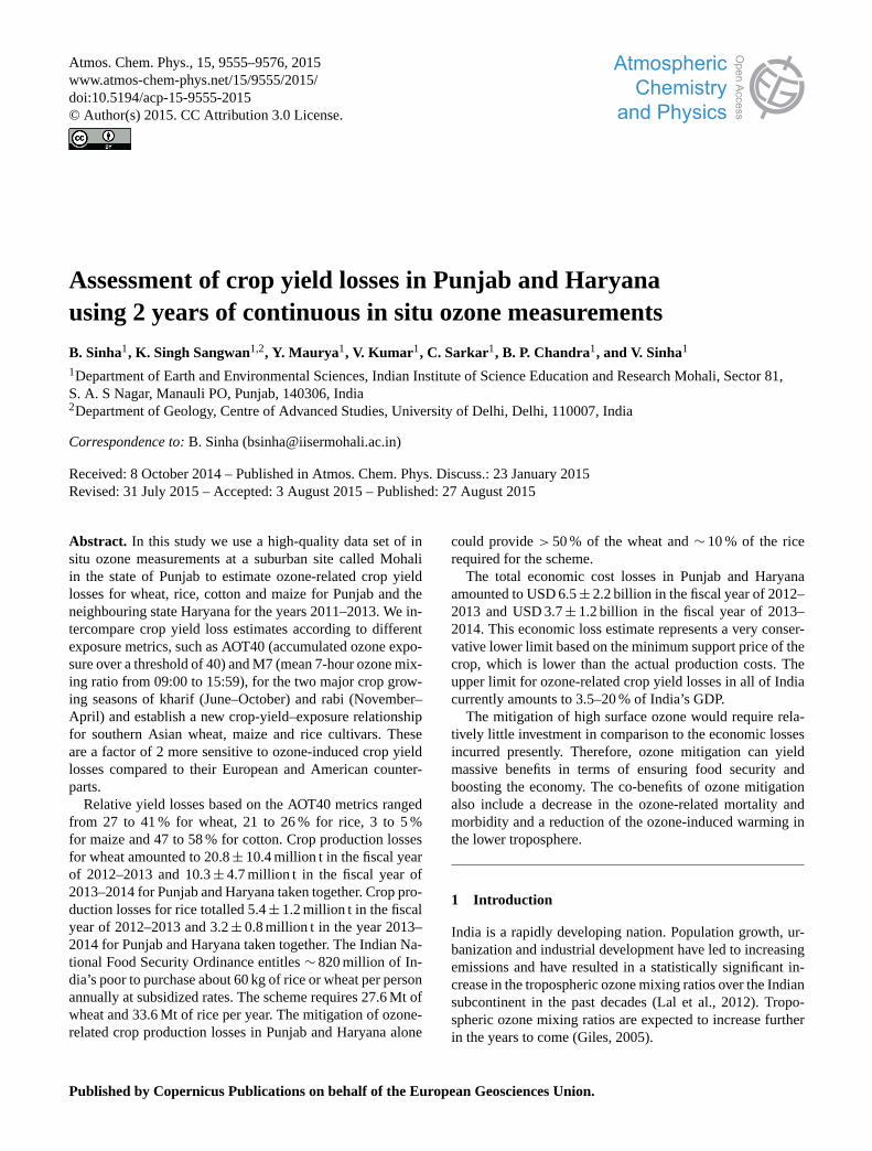
76.73◦ E; 310 m a.s.l.; Fig. 1). The measurement site is re-

www.atmos-chem-phys.net/15/9555/2015/ Atmos. Chem. Phys., 15, 9555–9576, 2015


gionally representative (Sinha et al., 2014) and located in the

north-west Indo-Gangetic Plain (NW IGP). Ozone measure-

ments from several other sites located in the IGP and the ad-

joining mountain regions (Fig. 1) will be discussed in detail

in Sect. 3.1 to demonstrate that the measurements obtained

at the facility are, indeed, regionally representative.

The measurement site is located inside a residential cam-

pus of around 1.25 km2 with 800–1000 residents. Local in-

fluence is expected to be significant only at low wind speeds

(< 1 m s−1), which occur only rarely (Sinha et al., 2014;

Pawar et al., 2015). The predominant daytime wind direction

is west to north-west during winter, summer and in the post-

monsoon season and south to south-east during the monsoon

season. The “fetch” region of air masses arriving at the site

is dominated by irrigated cropland (marked in light blue in

Fig. 1 in the state of Punjab, north-west of the site). During

the monsoon season, south-easterly winds bring air masses

from a fetch region covering irrigated cropland in the state of

Haryana, south-east of the site.

At the measurement site, inlets and meteorological mea-

surements are co-located atop the ambient air quality sta-

tion (AAQS) about 20 m above ground. A comprehensive de-

scription of the site and its representativeness for the north-

west Indo-Gangetic Plain can be found in Sinha et al. (2014),

and a thorough description of the meteorology of the site for

all seasons can be found in Pawar et al. (2015).

Ozone was measured using UV absorption photometry at

a time resolution of one measurement every minute, with

an accuracy that is better than 3 % and an overall uncer-

tainty of less than 6 %. Quality assurance of the large data

set was accomplished by regular calibrations using a NIST

traceable ozone primary standard generator and frequent zero

drift calibrations. Over the time span reported in this paper,

zero drift always remained below ±0.5 nmol mol−1 between

two subsequent zero drift calibrations. The drift of the cali-

bration factor during span calibrations was usually less than

±3 % and always below ±8 %, even after preventive mainte-

nance. A detailed description of the ozone measurements and

the supporting meteorological measurements can be found in

Sinha et al. (2014).

2.2 Calculation of ozone exposure metrics

We use two metrics to investigate the ozone exposure for

crops in Punjab and Haryana and derive southern-Asia-

specific exposure–yield relationships for wheat, maize and

rice. These are the mean daytime surface ozone (M7) and

accumulated exposure over a threshold of 40 nmol mol−1

(AOT40).

The Mx metric is defined as the mean daytime 7 (M7)

and 12 h (M12) surface ozone concentrations during daylight

hours, i.e. 09:00–15:59 and 08:00–19:59 LT respectively, in

the crop growing season (Hollaway et al., 2012).

M7=1

n

n∑i=1

[O3]i for 09:00–15:59LT (1)

AOT40 is defined as the sum of differences between

the hourly ozone concentrations and 40 nmol mol−1 dur-

ing the crop growing season (Fuhrer et al., 1997) for

[O3] > 40 nmol mol−1.

AOT40=

n∑i=1

([O3]i − 40) for [O3] > 40nmolmol−1 (2)

Of these parameters M7 gives equal importance to all mea-

surements and accounts for the yield losses due to ozone con-

centrations of less than 40 nmol mol−1, while AOT40 gives a

higher weight to high ozone mixing ratios (Tuovinen, 2000).

Hence, the former will perform better while evaluating plant

damage and yield losses at low ozone concentration, while

the latter will capture the effect of events with very high O3

mixing ratios on plant physiology and yields better (Holl-

away et al., 2012).

2.3 Missing data

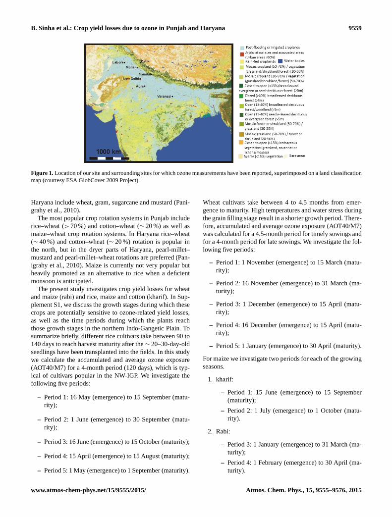
For any long-term data set, gaps in the data are inevitable due

to preventive maintenance, calibrations and technical prob-

lems that arise from time to time. The total number and

percentage of missing hourly average ambient data for each

month from October 2011 to November 2013 are listed in Ta-

ble 1. For calculating AOT40 and M7, continuous and com-

plete daytime data are required, since any missing value can

potentially lead to an underestimation of the real ozone ex-

posure. Hence, missing values need to be filled in. For short

data gaps of≤ 3 h arising due to zero drift calibration or span

calibrations we interpolated the measurements before and af-

ter the gap for filling in the missing values. Most gaps in the

time series are due to calibrations. For longer data gaps we

calculated the average diel ozone profile for the respective

month and for each missing hour filled in the monthly aver-

age ozone value of the respective hour. In most months less

than 5 % of the total hours were filled in. Only during the

monsoon season does the requirement to occasionally purge

the system with dry zero air lead to longer data gaps, and

up to 21 % of the hourly averages had to be filled using the

method described above.

2.4 Cropping seasons and major crops in Punjab and

Haryana

Rabi (winter season) and kharif (summer monsoon) are the

two main crop-growing seasons in northern India. In Punjab,

kharif crops include rice, cotton, maize, sugarcane and veg-

etables (Sharma and Sood, 2003). During rabi season wheat

is grown in almost all of Punjab (> 90 % of the area).

In Haryana, kharif crops include rice, cotton and sugarcane

and, in most of the unirrigated areas of Haryana, pearl mil-

let and sorghum (Panigrahy et al., 2010). Major rabi crops in



Figure 1. Location of our site and surrounding sites for which ozone measurements have been reported, superimposed on a land classification

map (courtesy ESA GlobCover 2009 Project).

Haryana include wheat, gram, sugarcane and mustard (Pani-

grahy et al., 2010).

The most popular crop rotation systems in Punjab include

rice–wheat (> 70 %) and cotton–wheat (∼ 20 %) as well as

maize–wheat crop rotation systems. In Haryana rice–wheat

(∼ 40 %) and cotton–wheat (∼ 20 %) rotation is popular in

the north, but in the dryer parts of Haryana, pearl-millet–

mustard and pearl-millet–wheat rotations are preferred (Pan-

igrahy et al., 2010). Maize is currently not very popular but

heavily promoted as an alternative to rice when a deficient

monsoon is anticipated.

The present study investigates crop yield losses for wheat

and maize (rabi) and rice, maize and cotton (kharif). In Sup-

plement S1, we discuss the growth stages during which these

crops are potentially sensitive to ozone-related yield losses,

as well as the time periods during which the plants reach

those growth stages in the northern Indo-Gangetic Plain. To

summarize briefly, different rice cultivars take between 90 to

140 days to reach harvest maturity after the∼ 20–30-day-old

seedlings have been transplanted into the fields. In this study

we calculate the accumulated and average ozone exposure

(AOT40/M7) for a 4-month period (120 days), which is typ-

ical of cultivars popular in the NW-IGP. We investigate the

following five periods:

– Period 1: 16 May (emergence) to 15 September (matu-

rity);

– Period 2: 1 June (emergence) to 30 September (matu-

rity);

– Period 3: 16 June (emergence) to 15 October (maturity);

– Period 4: 15 April (emergence) to 15 August (maturity);

– Period 5: 1 May (emergence) to 1 September (maturity).

Wheat cultivars take between 4 to 4.5 months from emer-

gence to maturity. High temperatures and water stress during

the grain filling stage result in a shorter growth period. There-

fore, accumulated and average ozone exposure (AOT40/M7)

was calculated for a 4.5-month period for timely sowings and

for a 4-month period for late sowings. We investigate the fol-

lowing five periods:

– Period 1: 1 November (emergence) to 15 March (matu-

rity);

– Period 2: 16 November (emergence) to 31 March (ma-

turity);

– Period 3: 1 December (emergence) to 15 April (matu-

rity);

– Period 4: 16 December (emergence) to 15 April (matu-

rity);

– Period 5: 1 January (emergence) to 30 April (maturity).

For maize we investigate two periods for each of the growing

seasons.

1. kharif:

– Period 1: 15 June (emergence) to 15 September

(maturity);

– Period 2: 1 July (emergence) to 1 October (matu-

rity).

2. Rabi:

– Period 3: 1 January (emergence) to 31 March (ma-

turity);

– Period 4: 1 February (emergence) to 30 April (ma-

turity).



Table 1. Total number (N ) of missing hourly average ambient

data (mh), total number of hours per month (th), percentage (%)

of missing hourly average ambient data for each month and number

of short (≤ 3 h) and long (> 3 h) data gaps.

Month mh/th Missing Short Long

(N/N) values gaps gaps

(%) (N) (N)

October 2011 2/672 0.3 2 0

November 2011 2/720 0.3 1 0

December 2011 4/744 0.5 2 0

January 2012 3/744 0.4 1 0

February 2012 1/696 0.1 1 0

March 2012 4/744 0.5 0 1

April 2012 45/720 6.3 2 1

May 2012 13/744 1.7 5 1

June 2012 3/720 0.4 2 0

July 2012 153/744 20.6 1 1

August 2012 57/744 7.7 2 1

September 2012 92/720 12.8 2 1

October 2012 8/744 1.1 2 1

November 2012 4/720 0.6 4 0

December 2012 33/744 4.3 2 2

January 2013 1/744 0.1 1 0

February 2013 1/672 0.1 1 0

March 2013 25/744 3.4 1 1

April 2013 5/720 0.7 2 0

May 2013 3/744 0.4 1 0

June 2013 108/720 15.0 1 3

July 2013 63/744 8.5 1 2

August 2013 73/744 9.8 1 1

September 2013 33/720 4.6 1 3

October 2013 42/744 5.6 1 1

November 2013 49/720 6.8 2 2

December 2013 2/672 0.3 2 0

January 2014 2/720 0.3 1 0

February 2014 4/744 0.5 2 0

3. For cotton, to cover the entire range of potential ozone

damage, three time windows are investigated:

– Period 1: 1 May–15 December; three pickings;

– Period 2: 31 May–15 December; three pickings;

– Period 3: 1 May–31 December; four pickings.

It should be noted, however, that these time windows do not

correspond to the same number of pickings and more pick-

ings will result both in higher yields and a longer time win-

dow in which plants can accumulate damage.

2.5 Relationships between ozone dose exposure and

yield

We derive specific exposure–yield relationships for Indian

wheat and rice cultivars using a two-pronged approach.

Firstly, we use our ozone measurements conducted at a

suburban site in Punjab and a number of field studies con-

ducted in the region that reported variations in the sowing

date of crops (Chahal et al., 2007; Jalota et al., 2008, 2009;

Mahajan et al., 2009; Brar et al., 2012; Buttar et al., 2013;

Ram et al., 2013), which lead to an unintentional change

in ozone exposure, and one study that reported co-located

yield and ozone measurements (Agrawal et al., 2003) to de-

rive an empirical exposure–yield relationship for rice and

wheat. The empirical field data support the need to revise the

exposure–yield relationship for Indian cultivars and demon-

strate that for rice optimizing, the sowing date can be a suit-

able strategy to minimize ozone exposure and maximize crop

yields.

Secondly, we derive India-specific exposure–yield rela-

tionships by plotting relative yields (RY) and ozone exposure

for all OTC studies on Indian cultivars reported in the peer-

reviewed literature and fitting the data to obtain an exposure–

yield relationship (Rai et al., 2007; Rai and Agrawal, 2008;

Rai et al., 2010; Singh et al., 2009; Singh and Agrawal, 2010;

Sarkar and Agrawal, 2010, 2012). For maize, only one OTC

study on two Indian cultivars has been conducted, and we use

the fit of these data to obtain an exposure–yield relationship

(Singh et al., 2014). We compare these exposure–yield rela-

tionships for rice and wheat with RY observed for cultivars

commonly grown in Pakistan and Bangladesh (Wahid et al.,

1995a, b; Maggs et al., 1995; Maggs and Ashmore, 1998;

Wahid, 2006; Akhtar et al., 2010a, b; Wahid et al., 2011)

to investigate to what extent the results can be extrapolated

to all of southern Asia. We refrain from including cultivars

popular in south-east Asia in our study, as they have been re-

ported to show a very different sensitivity to ozone exposure

(Sawada and Kohno, 2009). We provide an upper and lower

limit for RY and crop yield losses for a set of five differ-

ent sowing dates for rice and wheat, of three for cotton and

of two for rabi and kharif maize, using both exposure-dose–

response relationships established in several studies in the

west (Table 2) to provide a lower limit and our new India-

specific functions to provide an upper limit to the possible

loss.

We use both the old (Mills et al., 2007) AOT40-based

exposure–yield function and our revised AOT40-based rela-

tionship to calculate crop production losses and economic

cost losses and contrast the two.

2.6 Yield loss and economic loss calculations

Table 2 summarizes the ozone exposure-dose–response rela-

tionships for relative yield loss (RYL) for wheat, rice, maize



Table 2. Exposure–relative-yield (RY) relationships established in the literature and comparison with our own exposure–relative-yield rela-

tionships. RY stands for relative yield.

Crop Index Exposure–RY relationship References

Rice M7 RY= e−(M7/202)2.47/e−(25/202)2.47

Adams et al. (1989)

AOT40 RY=−0.0000039×AOT40+ 0.94 Mills et al. (2007)

POD10 RY= 0.996− 0.487×POD10 Yamaguchi et al. (2014); ozone-resistant rice

M7 RY= e−(M7/86)2.5/e−(25/86)2.5

this study;Indian rice cultivars

AOT40 RY=−0.00001×AOT40+ 0.95 this study;Indian rice cultivars

Wheat M7 RY= e−(M7/137)2.34/e−(25/137)2.34

Lesser et al. (1990); winter wheat

M7 RY= e−(M7/114)1.8/e−(25/114)1.8

Heck et al. (1984b); winter wheat

M7 RY= e−(M7/186)3.2/e−(25/186)3.2

Adams et al. (1989); spring wheat


POD6 RY= 1− 0.038×POD6 Mills et al. (2011b)

M7 RY= e−(M7/62)4.5/e−(25/62)4.5

this study;Indian wheat cultivars

AOT40 RY=−0.000026×AOT40+ 1.01 this study;Indian wheat cultivars

Maize M7 RY= e−(M7/158)3.69/e−(25/158)3.69

Heck et al. (1984b)


AOT40 RY=−0.0000067×AOT40+ 1.03 Indian maize; Singh et al. (2014)

Cotton AOT40 RY=−0.000016×AOT40+ 1.07 Mills et al. (2007)

M7 RY= e−(M7/152)2.2/e−(25/152)2.2

Heck et al. (1984b)

and cotton based on AOT40 and M7 values collected from

the peer-reviewed literature.

All the ozone exposure-dose–response relationships pre-

viously reported in the literature are based on field studies

conducted in the USA or in Europe. Relative yield loss is de-

fined as the crop yield reduction from the theoretical yield

that would have resulted without O3-induced damages (Avn-

ery et al., 2011a), calculated using Eqs. (3) and (4):

RYLi = 1−RYi, (3)

CPLi =RYLi

1−RYLi

×CPi, (4)

where RYi stands for relative yield in the year i, CPLi stands

for crop production loss in the year i and CPi stands for the

crop production of the same year. The crop production per

fiscal year was taken from the database of the Directorate of

Economics and Statistics (2013).

Economic cost loss (ECL) for any crop is defined as the

financial loss due to O3-induced damage in a given finan-

cial year. The minimum ECL is calculated for different crops

based on corresponding minimum support prices (MSPs) of

the same fiscal year using the following equation:

ECLi = CPLi ×MSPi . (5)

The MSPs are recommended by Commission for Agriculture

Costs and Prices (Directorate of Economics and Statistics,

2013) and are announced by the Government of India at the

beginning of each season for each year. These prices are de-

fined as the fixed price at which government purchases crops

from the farmers. All our crops of interest come under the

MSP valuation process. It should be noted, however, that the

MSP is typically approximately 50 % less than the market

value of the crop and often lower than the production costs.

The upper limit for the ECL is calculated using the relation-

ship between CPL due to deficient monsoon rains and the

Indian GDP established by Gadgil and Gadgil (2006) using

the following equation:

ECLi[%GDP] = RYLi[%]× 0.36. (6)

3 Results and discussions

3.1 Ozone seasonal cycle and monthly ozone exposure

indices

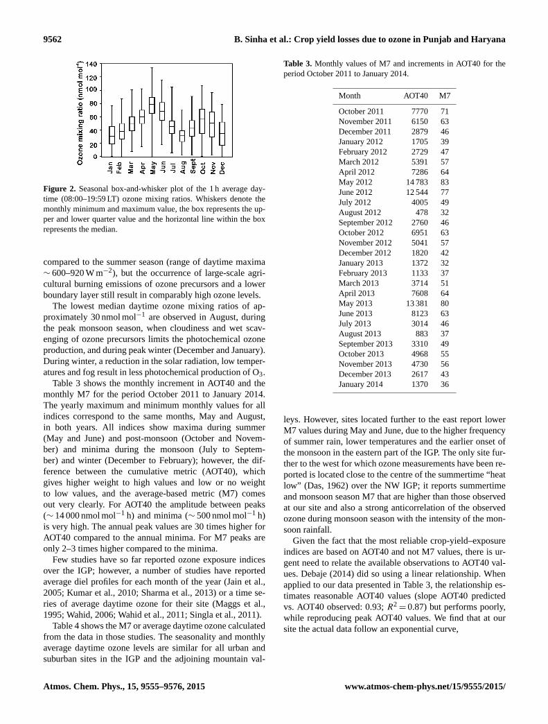
Figure 2 shows the seasonal box-and-whisker plot of the

daytime (08:00–19:59 LT) 1 h average ozone mixing ratios

for the period from October 2011 to January 2014. The

highest ozone levels are observed in the summer season in

April, May and June, with median ozone mixing ratios of

60–80 nmol mol−1 and peak ozone mixing ratios of approxi-

mately 130 nmol mol−1. This is expected, as conditions such

as high temperature, low humidity and high solar radiation

favour the photochemical production of O3 regionally.

After summer, the next highest ozone levels are observed

during the post-monsoon season (October and November),

with median ozone mixing ratios of 50–60 nmol mol−1. The

post-monsoon season is characterized by lower levels of so-

lar radiation (range of daytime maxima ∼ 480–720 W m−2)



Figure 2. Seasonal box-and-whisker plot of the 1 h average day-

time (08:00–19:59 LT) ozone mixing ratios. Whiskers denote the

monthly minimum and maximum value, the box represents the up-

per and lower quarter value and the horizontal line within the box

represents the median.

compared to the summer season (range of daytime maxima

∼ 600–920 W m−2), but the occurrence of large-scale agri-

cultural burning emissions of ozone precursors and a lower

boundary layer still result in comparably high ozone levels.

The lowest median daytime ozone mixing ratios of ap-

proximately 30 nmol mol−1 are observed in August, during

the peak monsoon season, when cloudiness and wet scav-

enging of ozone precursors limits the photochemical ozone

production, and during peak winter (December and January).

During winter, a reduction in the solar radiation, low temper-

atures and fog result in less photochemical production of O3.

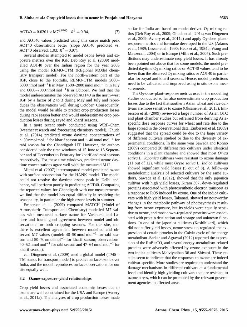
Table 3 shows the monthly increment in AOT40 and the

monthly M7 for the period October 2011 to January 2014.

The yearly maximum and minimum monthly values for all

indices correspond to the same months, May and August,

in both years. All indices show maxima during summer

(May and June) and post-monsoon (October and Novem-

ber) and minima during the monsoon (July to Septem-

ber) and winter (December to February); however, the dif-

ference between the cumulative metric (AOT40), which

gives higher weight to high values and low or no weight

to low values, and the average-based metric (M7) comes

out very clearly. For AOT40 the amplitude between peaks

(∼ 14 000 nmol mol−1 h) and minima (∼ 500 nmol mol−1 h)

is very high. The annual peak values are 30 times higher for

AOT40 compared to the annual minima. For M7 peaks are

only 2–3 times higher compared to the minima.

Few studies have so far reported ozone exposure indices

over the IGP; however, a number of studies have reported

average diel profiles for each month of the year (Jain et al.,

2005; Kumar et al., 2010; Sharma et al., 2013) or a time se-

ries of average daytime ozone for their site (Maggs et al.,

1995; Wahid, 2006; Wahid et al., 2011; Singla et al., 2011).

Table 4 shows the M7 or average daytime ozone calculated

from the data in those studies. The seasonality and monthly

average daytime ozone levels are similar for all urban and

suburban sites in the IGP and the adjoining mountain val-

Table 3. Monthly values of M7 and increments in AOT40 for the

period October 2011 to January 2014.

Month AOT40 M7

October 2011 7770 71

November 2011 6150 63

December 2011 2879 46

January 2012 1705 39

February 2012 2729 47

March 2012 5391 57

April 2012 7286 64

May 2012 14 783 83

June 2012 12 544 77

July 2012 4005 49

August 2012 478 32

September 2012 2760 46

October 2012 6951 63

November 2012 5041 57

December 2012 1820 42

January 2013 1372 32

February 2013 1133 37

March 2013 3714 51

April 2013 7608 64

May 2013 13 381 80

June 2013 8123 63

July 2013 3014 46

August 2013 883 37

September 2013 3310 49

October 2013 4968 55

November 2013 4730 56

December 2013 2617 43

January 2014 1370 36

leys. However, sites located further to the east report lower

M7 values during May and June, due to the higher frequency

of summer rain, lower temperatures and the earlier onset of

the monsoon in the eastern part of the IGP. The only site fur-

ther to the west for which ozone measurements have been re-

ported is located close to the centre of the summertime “heat

low” (Das, 1962) over the NW IGP; it reports summertime

and monsoon season M7 that are higher than those observed

at our site and also a strong anticorrelation of the observed

ozone during monsoon season with the intensity of the mon-

soon rainfall.

Given the fact that the most reliable crop-yield–exposure

indices are based on AOT40 and not M7 values, there is ur-

gent need to relate the available observations to AOT40 val-

ues. Debaje (2014) did so using a linear relationship. When

applied to our data presented in Table 3, the relationship es-

timates reasonable AOT40 values (slope AOT40 predicted

vs. AOT40 observed: 0.93; R2= 0.87) but performs poorly,

while reproducing peak AOT40 values. We find that at our

site the actual data follow an exponential curve,



AOT40= 0.0201×M73.0765 R2= 0.94, (7)

and AOT40 values predicted using this curve match peak

AOT40 observations better (slope AOT40 predicted vs.

AOT40 observed: 1.03; R2= 0.97).

Several studies attempted to model ozone levels and ex-

posure metrics over the IGP. Deb Roy et al. (2009) mod-

elled AOT40 over the Indian region for the year 2003

using the model REMO-CTM (REgional MOdel chem-

istry transport model). For the north-western part of the

IGP, close to the foothills, REMO-CTM models 5000–

6000 nmol mol−1 h in May, 1500–2000 nmol mol−1 h in July

and 6000–7000 nmol mol−1 h in October. We find that the

model underestimates the observed AOT40 in the north-west

IGP by a factor of 2 to 3 during May and July and repro-

duces the observations well during October. Consequently,

the model would be able to predict crop production losses

during rabi season better and would underestimate crop pro-

duction losses during zayad and kharif seasons.

In a more recent study conducted using WRF-Chem

(weather research and forecasting chemistry model), Ghude

et al. (2014) predicted ozone daytime concentrations of

∼ 50 nmol mol−1 for kharif season and ∼ 40 nmol mol−1 for

rabi season for the Chandigarh UT. However, the authors

considered only the time windows of 15 June to 15 Septem-

ber and of December to February for kharif and rabi seasons

respectively. For these time windows, predicted ozone day-

time concentrations agree well with the measured M12.

Mittal et al. (2007) intercompared model-predicted ozone

with surface observation for the HANK model. The model

could not resolve the daytime ozone peak in Delhi and,

hence, will perform poorly in predicting AOT40. Comparing

the reported values for Chandigarh with our measurements,

we find that the model has equal difficulty in resolving the

seasonality, in particular the high ozone levels in summer.

Emberson et al. (2009) compared MATCH (Model of

Atmospheric Transport and Chemistry)-modelled M7 val-

ues with measured surface ozone for Varanarsi and La-

hore and found good agreement between model and ob-

servations for both cropping seasons. For our site, too,

there is excellent agreement between modelled and ob-

served M7 values (model: 40–50 nmol mol−1 for rabi sea-

son and 50–70 nmol mol−1 for kharif season; observations:

40–52 nmol mol−1 for rabi season and 47–64 nmol mol−1 for

kharif season).

van Dingenen et al. (2009) used a global model (TM5 –

TM stands for transport model) to predict surface ozone over

India, and the model reproduces surface observations for our

site equally well.

3.2 Ozone-exposure–yield relationships

Crop yield losses and associated economic losses due to

ozone are well constrained for the USA and Europe (Avnery

et al., 2011a). The analyses of crop production losses made

so far for India are based on model-derived O3 mixing ra-

tios (Deb Roy et al., 2009; Ghude et al., 2014; van Dingenen

et al., 2009; Avnery et al., 2011a) and apply O3-dose–plant-

response metrics and formulae developed in the US (Adams

et al., 1989; Lesser et al., 1990; Heck et al., 1984b; Wang and

Mauzerall, 2004) or in Europe (Mills et al., 2007). Such pre-

dictions may underestimate crop yield losses. It has already

been pointed out above that for some models, the model pre-

dicted daytime O3 mixing ratios or AOT40 values tend to be

lower than the observed O3 mixing ratios or AOT40 in partic-

ular for zayad and kharif seasons. Hence, model predictions

need to be validated and improved using in situ ozone mea-

surements.

The O3-dose–plant-response metrics used in the modelling

studies conducted so far also underestimate crop production

losses due to the fact that southern Asian wheat and rice cul-

tivars are more sensitive to ozone (Oksanen et al., 2013). Em-

berson et al. (2009) reviewed a large number of Asian OTC

and plant chamber studies but refrained from deriving Asia-

specific dose response curves for wheat and rice due to the

large spread in the observational data. Emberson et al. (2009)

suggested that the spread could be due to the large variety

of different cultivars studied or due to the diversity of ex-

perimental conditions. In the same year Sawada and Kohno

(2009) compared 20 different rice cultivars under identical

conditions in a plant chamber and showed that most Oryza

sativa L. Japonica cultivars were resistant to ozone damage

(11 out of 12), while most Oryza sativa L. Indica cultivars

showed significant yield losses (5 out of 8). A follow-up

metabolomic analysis of selected cultivars by the same au-

thors, Sawada et al. (2012), showed that the only japonica

cultivar with high yield losses, Kirara 397, down-regulated

proteins associated with photosynthetic electron transport as

a response to ROS induced by ozone. One of the indica culti-

vars with high yield losses, Takanari, showed no noteworthy

changes in the metabolic pathway of photosynthesis result-

ing from ozone exposure, but its yields were equally sensi-

tive to ozone, and most down-regulated proteins were associ-

ated with protein destination and storage and unknown func-

tions. In one of the japonica cultivars (Koshihikari), which

did not suffer yield losses, ozone stress up-regulated the ex-

pression of certain proteins in the Calvin cycle of the energy

metabolism. Sarkar and Agrawal (2012) reported the expres-

sion of the RuBisCO, and several energy-metabolism-related

proteins were adversely affected by ozone exposure in the

two indica cultivars Malviyadhan 36 and Shivani. These re-

sults seem to indicate that the responses to ozone are indeed

cultivar-specific. More studies are required to understand the

damage mechanisms in different cultivars at a fundamental

level and identify high-yielding cultivars that are resistant to

ozone stress, which can be promoted by the relevant govern-

ment agencies in affected areas.



Table 4. Comparison of the average monthly ozone exposure indices observed at a suburban site in Mohali with measurements at other urban

(superscript letters a–h) and suburban (superscript i and j) sites in the IGP and nearby remote mountain (superscript l) and suburban valley

(superscript k) sites indicated in Fig. 1.

Site Mohalia Mohalia Lahoreb Lahorec, d New New Agrag Agrah Varanarsii, j Kulluk Nainitall

Delhie Delhif

Years 2011– 2011– 1992– 2003– 2001 1997– 2000– 2008– 2003– 2010 2006–

2014 2014 1993 2004; 2004 2002 2009 2005 2008

2007

Index M7 M12 10:00– 08:00– M7 11:00– 09:00– 09:00– M12 M7 M7

16:00 16:00 18:00 18:00 17:00

January 36 32 40 66 35 32 56 28 35 46 38

February 42 37 48 80 57 46 11 45 41 53 42

March 54 48 47 92 60 50 45 52 48 70 43

April 64 58 52 96 62 55 19 60 53 65 61

May 82 74 – – 50 55 19 61 56 77 63

June 70 66 61 95 41 41 27 46 51 62 41

July 48 45 43 93 51 30 16 22 34 48 27

August 35 31 48 84 30 24 11 12 25 – 23

September 48 42 55 69 45 30 25 29 29 – 27

October 63 51 58 60 56 40 36 42 42 58 40

November 59 46 33 53 53 41 53 51 41 53 43

December 44 38 36 57 56 34 30 34 37 53 39

a this study; b Maggs et al. (1995); c Wahid (2006); d Wahid et al. (2011); e Jain et al. (2005); f Ghude et al. (2008); g Satsangi et al. (2004); h Singla et al. (2011); i Tiwari et al.

(2008); j Rai and Agrawal (2008); k Sharma et al. (2013); l Kumar et al. (2010). Except in the case of values from this study, from Ghude et al. (2008) and from Tiwari et al. (2008),

values in the table were calculated from the available diel profiles or time series plots.

Figure 3. Empirical correlation of rice yields and ozone exposure indices for field studies with variations in sowing date. Ozone exposure

for rice sown on different dates has been calculated using our data (Table 5). Yield data for rice have been taken from the peer-reviewed

literature (Chahal et al., 2007; Jalota et al., 2009; Mahajan et al., 2009; Brar et al., 2012). Error bars on the x axis show the variance in the

ozone exposure metrics for the same growth period (see Supplement S1 for definition) for different years. Error bars on the y axis show the

variance in the yield obtained. Variance is introduced by replicating the study on several test plots (in different districts; plots with different

soil properties using different cultivars) and in several years or by transplanting seedlings with a different age at the time of transplanting.

3.2.1 Rice

Figure 3 shows the empirical correlation of rice yields and

ozone exposure indices for field studies with variations in

sowing in Punjab and Haryana. There is a significant trend

in the reported crop yields as a function of ozone exposure

indices (Fig. 3; R2= 0.58 for M7 and R2

= 0.57 for AOT40).

For rice, late sowing (1 June) and late transplantation (1 July)

leads to the lowest relative yield losses (18 %), while early

sowing (1 April) and transplantation (1 May) doubles ozone-

related yield losses (35 %; Table 5).

Figure 4 compares the empirical ozone-exposure–

response curve derived from the field data presented in Fig. 3

(solid line) with RY values determined in OTC studies con-



Table 5. Ozone exposure according to different exposure indices and relative yields for rice. Data for the five periods used to plot Fig. 3 are

provided in the table. Periods (P) 1–3 correspond to the periods in which rice is usually grown in Punjab and Haryana, and the average yield

loss of these three periods is used to calculate crop production loss and economic loss for each fiscal year.

Time AOT40 M7 RYAOT40 RYM7 RYAOT40 RYM7

Mills et al. Adams et al. Indian Indian

(2007) (1989) OTC OTC

studies studies

2012 P1 25 641 55 0.84 0.97 0.69± 0.05 0.75± 0.06

2012 P2 19 788 51 0.86 0.97 0.75± 0.04 0.80± 0.06

2012 P3 16 715 49 0.87 0.98 0.78± 0.04 0.82± 0.06

2012 P4 35 640 64 0.80 0.95 0.59± 0.06 0.65± 0.07

2012 P5 31 853 60 0.82 0.96 0.63± 0.05 0.70± 0.07

Average P1–3 20 715 52 0.86 0.97 0.74± 0.04 0.79± 0.06

2013 P1 20 839 53 0.86 0.97 0.74± 0.04 0.78± 0.06

2013 P2 15 330 49 0.88 0.98 0.80± 0.04 0.82± 0.05

2013 P3 12 623 47 0.89 0.98 0.82± 0.03 0.84± 0.05

2013 P4 29 259 60 0.83 0.96 0.66± 0.05 0.70± 0.07

2013 P5 25 498 56 0.84 0.96 0.70± 0.05 0.74± 0.06

Average P1–3 16 264 49 0.88 0.98 0.79± 0.04 0.81± 0.06

Figure 4. Comparison of the empirical exposure–response relationship based on field data (solid line) with OTC studies conducted in India

(squares with dash and dot fit) and Pakistan (diamonds, not included in line fit). Large diamonds indicate studies conducted on basmati; all

other studies were conducted on paddy. Circles show plant chamber studies on Bangladeshi rice cultivars conducted in Japan, and the dashed

line delineates the European (AOT40; Mills et al., 2007) and American (M7; Adams et al., 1989) dose–response relationship. In all studies

presented in this figure, rice plants were exposed to elevated ozone from the date of transplantation until harvest.

ducted in India (squares, dash and dot line fit) and Pakistani

Punjab (diamonds). For studies that did not report AOT40

but did report monthly or seasonal M7, M8 or M12, AOT40

was calculated using the relationship between the respective

index and AOT40 at our site. For M7, all data points of OTC

studies lie close to the line derived from the empirical rela-

tionship between crop yields and ozone exposure in Punjab.

The fit for the OTC studies gives a similar slope to the lin-

ear fit of the yield data. Since OTC studies compare yield

losses of plants exposed to ozone with those of plants grown

under identical conditions but in clean filtered air, the ozone-

exposure–response curve derived from OTC studies of Indian

cultivars provides the most accurate estimate of the RYL. A

new RYL equation for Indian rice cultivars (Table 2) is de-

rived by fitting all relative yields for Indian cultivars from

OTC studies (Fig. 4). We calculate relative yields for all five

reference periods defined in Supplement S1, using both the

old (Mills et al., 2007; Adams et al., 1989) and the revised

RYL relationships.

It is clear from Fig. 4 and Table 5 that the RY curve derived

by Adams et al. (1989) significantly overestimate the RY of

Oryza sativa L. Indica cultivars planted in the IGP, and it is



Figure 5. Empirical correlation of wheat yields and ozone exposure indices for field studies with variations in sowing date. Ozone exposure

for wheat sown on different dates has been calculated using our data (Table 6). Yield data for wheat have been taken from the peer-reviewed

literature (Agrawal et al., 2003; Chahal et al., 2007; Jalota et al., 2008; Coventry et al., 2011; Buttar et al., 2013; Ram et al., 2013). Agrawal

et al. (2003) reported co-located measurements of ozone exposure and yields for a number of urban locations that included residential areas

and kerb site locations, where NO titration leads to low wintertime ozone levels. Other studies reported yields corresponding to different

sowing dates. The yield data have been positioned to conform with the emergence dates (Periods 1 to 5) defined in Supplement S1. Error bars

on the x axis show the variance in the ozone exposure metrics for the same growth period (see Supplement S1 for definition) for different

years. Error bars on the y axis show the variance in the yield obtained. Variance is introduced by replicating the study on several test plots,

in multiple years or varying growing conditions and by the number of irrigations and or the tillage practices.

interesting to note that there seems to be an east–west gra-

dient in the sensitivity of local cultivars to ozone exposure.

Bangladeshi cultivars showed the lowest sensitivity and high-

est relative yields, though this could be due to the fact that the

study was conducted in the sheltered environment of a plant

chamber. Pakistani cultivars showed the highest sensitivity to

ozone exposure and the lowest relative yields.

Crop production losses calculated using the equation de-

rived based on American studies (Adams et al., 1989) under-

estimate crop production losses in southern Asia by approx-

imately 20–30 % (Table 5). For AOT40 both the empirical

relationship between crop yields and ozone exposure and the

OTC studies conducted in India lead to line fits with similar

slopes; however, OTC studies show an intercept of 0.95 for

AOT40= 0, indicating that in southern Asia ozone levels be-

low 40 nmol mol−1 damage local paddy cultivars. While de-

riving the empirical relationship from field data, the RY for

AOT40= 0 was defined as 1 due to the absence of clean-air

controls. The slope of the revised equation is steeper than the

slope reported by Mills et al. (2007), and the intercept of the

Indian OTC studies is also lower; hence RY and crop pro-

duction losses calculated using the equation derived based

on European studies underestimate crop production losses

in southern Asia by approximately 5–15 % (Table 5). Ta-

ble 5 summarizes relative yields for the five reference periods

(which correspond to different sowing dates) and intercom-

pares RY calculated using the new equation with RY calcu-

lated using the old relationships. It can be noted that AOT40

shows a better degree of agreement between the exposure–

yield relationship of Mills et al. (2007) and the exposure–

yield relationship for Indian cultivars (Table 5). The dif-

ference between the two is generally ∼ 10 %. On the other

hand, M7 shows a lower degree of agreement between the

exposure–yield relationship of Adams et al. (1989) and the

exposure–yield relationship for Indian cultivars (Table 5).

The difference between the two is ∼ 20 %. Using the re-

vised relationship, relative yields calculated using the M7

and AOT40 metrics agree within the uncertainty, while pre-

viously the discrepancy between the crop yield losses cal-

culated using M7 and AOT40 metrics exceeded 10 %. Our

revised ozone exposure crop yield relationships show signif-

icantly lower relative yields than those using the previous

exposure–response relationships. This can be attributed to

the variety of cultivars. The Indian cultivars are more sen-

sitive to O3 exposure.

3.2.2 Wheat

Figure 5 shows the empirical correlation of wheat yields and

ozone exposure indices for field studies with variations in

sowing in Punjab and Haryana. There is a significant de-

crease in yield as a function of increasing ozone exposure

(Fig. 5) for both ozone exposure indices (R2= 0.55 of M7

and R2= 0.7 for AOT40). For AOT40 the relative yield is

determined with respect to the yield that would have been

obtained for AOT40= 0.

Figure 6 compares the empirical ozone-exposure–

response curve derived from field data (solid line) with RYL



Table 6. Ozone exposure according to different exposure indices and relative yields for wheat. Data for the five periods used to plot Fig. 5

are provided in the table. Period 2 (P2) and Period 3 (P3) correspond to the periods in which wheat is usually grown in Punjab and Haryana

in the rice–wheat cropping cycle, while Period 4 (P4) and 5 (P5) correspond to the cotton–wheat cropping cycle. The average yield loss of

the rice–wheat cycle is used to calculate crop production loss and economic loss for each fiscal year as most of the area is cultivated in the

rice–wheat cropping system.

Time AOT40 M7 RYAOT40 RYM7 RYM7 RYAOT40 RYM7

Mills Lesser Heck Indian Indian

et al. et al. et al. OTC OTC

(2007) (1990) (1984b) studies studies

2012 P1 15 843 49 0.73 0.93 0.85 0.60± 0.10 0.74± 0.07

2012 P2 15 807 49 0.74 0.93 0.86 0.60± 0.10 0.75± 0.07

2012 P3 16 168 49 0.73 0.93 0.86 0.59± 0.10 0.75± 0.07

2012 P4 14 754 49 0.75 0.93 0.85 0.63± 0.10 0.74± 0.07

2012 P5 17 110 52 0.71 0.92 0.84 0.57± 0.11 0.69± 0.07

Average P2–3 15 987 49 0.73 0.93 0.86 0.59± 0.10 0.75± 0.07

2013 Period-1 11 384 42 0.81 0.96 0.91 0.71± 0.09 0.88± 0.05

2013 Period-2 9887 40 0.83 0.96 0.92 0.75± 0.08 0.90± 0.05

2013 Period-3 11 375 41 0.81 0.96 0.91 0.71± 0.09 0.88± 0.05

2013 Period-4 10 012 41 0.83 0.96 0.91 0.75± 0.08 0.89± 0.05

2013 Period-5 13 817 46 0.77 0.94 0.88 0.65± 0.10 0.81± 0.06

Average P2–3 10 631 41 0.82 0.96 0.91 0.73± 0.08 0.89± 0.05

Figure 6. Comparison of the empirical exposure–response relationship based on field data (solid line) with OTC studies conducted in

India (squares with line fit) and Pakistan (diamonds, not included in line fit). Circles show plant chamber studies on Bangladeshi wheat

cultivars conducted in Japan. The exposure–response relationship based on American and European studies is plotted in the same graph for

comparison. In all studies on southern Asian cultivars, wheat was exposed to elevated ozone levels from emergence to harvest, while the

European and American exposure–response curves include data sets acquired on wheat crops that were exposed to elevated ozone during the

last 3 months prior to harvest.

relationships reported in the literature (Mills et al., 2007;

Heck et al., 1984b; Lesser et al., 1990; Adams et al., 1989)

and with OTC studies conducted in India (squares, dash and

dot line) and Pakistani Punjab (diamonds). For studies that

did not report AOT40 but did report monthly or seasonal

averaged M7 or M12, AOT40 was estimated. For M7 most

data points of OTC studies with Indian cultivars lie close

to the line derived from the empirical relationship between

crop yields and ozone exposure in Punjab. However, the

exposure–response relationship for wheat can only be appro-

priately described by fitting a Weibull function. Since OTC

studies compare yield losses of plants exposed to ozone with

those of plants grown under identical conditions but in clean

filtered air, the ozone exposure–response curve derived from

OTC studies of Indian cultivars provides the most accurate

estimate of the RYL. A new RYL equation for Indian wheat

cultivars (Table 2) is derived by fitting all relative yields for

Indian cultivars from OTC studies (Fig. 6). We calculate rel-



ative yields for all five reference periods defined in Sup-

plement S1 both using the old (Mills et al., 2007; Adams

et al., 1989) and the revised RYL relationships. It is clear

from Fig. 6 that the RY curves for winter wheat derived by

Lesser et al. (1990) and Heck et al. (1984b) overestimates

the RY of most Triticum aestivum L. cultivars planted in the

IGP. For Triticum aestivum L. there is no significant trend

between cultivars planted in different countries. Crop pro-

duction losses calculated using the M7 index and the equa-

tion derived based on American studies (Lesser et al., 1990;

Heck et al., 1984b) underestimates crop production losses in

southern Asia by approximately 10 and 20 % for the equation

of Heck et al. (1984b) and Lesser et al. (1990) respectively

(Table 6).

For AOT40 both the empirical relationship between crop

yields and ozone exposure and the OTC studies conducted in

India lead to line fits with similar slopes and intercepts. The

slope obtained in the current study is steeper than the slope

reported by Mills et al. (2007), although a limited number of

cultivars planted in the IGP show an exposure–RY relation-

ship similar to that reported by Mills et al. (2007). Cultivars

with lower sensitivity to ozone include Bijoy (Akhtar et al.,

2010a), Inqilab-91, Punjab-96 and Pasban-90 (Wahid, 2006),

HUW234, PBW343 and Sonalika (Singh et al., 2009; Sarkar

and Agrawal, 2010). For HUW468 the sensitivities obtained

by Singh et al. (2009) and Singh and Agrawal (2010) dif-

fer. However, for most cultivars crop production losses cal-

culated using the equation derived based on European stud-

ies underestimate crop production losses in southern Asia.

Table 6 summarizes relative yields that are obtained by our

calculation. For AOT40 the exposure–yield relationship of

Mills et al. (2007) and the exposure–yield relationship for

Indian cultivars (Table 6) differ by ∼ 10–15 %. For M7 the

exposure–yield relationship of Lesser et al. (1990) overes-

timates the yields by ∼ 20 % and the exposure–yield rela-

tionship of Heck et al. (1984b) by ∼ 10 % (Table 6). Af-

ter the revision, relative yields calculated using the M7 and

AOT40 metrics still show a∼ 15 % discrepancy although the

estimates do overlap within the combined uncertainty. The

quality of the fit for M7 is better than the fit for AOT40;

however, given the very steep slope of the M7 curve at

> 35 nmol mol−1 and the large number of points below the

fit line for higher M7 values, it is credible that cultivars with

such a sensitivity to ozone would respond very strongly to

even a few days with extremely high ozone, and such be-

haviour will only be captured by the AOT40 index. Daytime

peaks with∼ 70–100 nmol mol−1 are observed in March and

April (Fig. 2) during the grain filling stage of the plants, and

the M7 for the full growth period does not capture such ex-

treme events. AOT40 is the better indicator to accurately re-

flect exposure when the variance of the amplitude of day-

time peak ozone is high. Picchi et al. (2010) reported a

high sensitivity of wheat cultivars to ozone exposure during

the grain filling stage, and our observations agree well with

their finding. Therefore, for southern Asian wheat cultivars,

Table 7. Ozone exposure according to different exposure indices

and relative yields for cotton. Period 1 (P1) and Period 2 (P2) cor-

respond to the periods in which cotton is usually grown.

Time AOT40 M7 RYAOT40 RYM7

Mills Heck

et al. et al.

(2007) (1984b)

2012 P1 47926 57 0.30 0.91

2012 P2 33 728 53 0.53 0.91

2012 P3 48 342 56 0.30 0.92

Average P1–2 40 825 55 0.42 0.91

2013 P1 40 029 55 0.43 0.92

2013 P2 27 312 51 0.63 0.92

2013 P3 41 046 53 0.41 0.93

Average P1–2 33 670 53 0.53 0.92

the revised exposure–response curve using AOT40 will pro-

vide the best estimate of the crop production losses. Our re-

vised ozone-exposure–crop-yield relationships show signifi-

cantly lower relative yields than those obtained by exposure–

response relationships used previously (−15 % for AOT40).

This can be attributed to the variety of cultivars. Most In-

dian cultivars are more sensitive to a high O3 concentration,

although a few individual cultivars show higher resistance.

3.2.3 Cotton

Cotton yield data for this region have only been reported in

two studies (Jalota et al., 2008; Buttar et al., 2013), and OTC

studies on cotton in India have not been conducted to date.

Buttar et al. (2013) reported yields for different numbers of

pickings (Periods 2 and 3), and hence his observations cannot

be used to investigate the crop response to ozone. Exposure–

yield relationships acquired abroad indicate that cotton is po-

tentially extremely sensitive to ozone-induced damage. The

yield data from India show very high variability and no sig-

nificant influence of ozone on yields when the results are av-

eraged over 2 years (Jalota et al., 2008). However, there is

a significant intra- and interannual variability in yields as a

function of rainfall reported from the site on which the crop

was grown (Jalota et al., 2008). Since the crop was irrigated

sufficiently, this yield dependence on rain should not be re-

lated to drought stress. Ozone levels in Punjab during the

monsoon season are strongly influenced by the wet scav-

enging of precursors and cloudiness; hence, rain spells can

be taken as a proxy for times of low photochemical ozone

production. The lowest yields were observed for Period 1

sowings in 2004 that were affected by a prolonged dry spell

from 60 to 100 days after sowing. This corresponds to the

period of maximum square production and peak bloom in

a cotton plant. In 2005 the same Period 1 sowings received

regular rain (every 5–7 days) in the same time period (to-



tal of 400 mm between 60 to 100 days after sowing) and

showed the highest yields (2.4 times the yield of the previous

year on average). The Period 2 sowings in 2005 received rain

40 to 80 days after sowing but were subjected to a dry spell

during the second half of the square production and peak

bloom period. Observed yields were 1.9 times higher com-

pared to the plants that were subjected to a dry spell during

the entire period. Period 2 sowings in 2004 received a short

(∼ 7-day) rain spell around 80 days after sowings during the

peak square production period and showed yields that were

1.4 times the dry-spell yields. Considering the average differ-

ence between dry-spell and rain spell M7 of approximately

10–20 nmol mol−1, the observations described above seem to

suggest a strong sensitivity of the plant to ozone levels during

square production and peak bloom (60–100 days after sow-

ing), but it is difficult to separate the effect of yield losses due

to adverse meteorological conditions from that due to ozone

exposure. In the absence of dedicated OTC fumigation stud-

ies conducted in India that separate the two effects, we use

the relationship of Mills et al. (2007) and Heck et al. (1984b)

to calculate relative yields (Table 7).

For cotton there are extreme differences of 30–60 % be-

tween the relative yields calculated using AOT40 (Mills

et al., 2007) and M7 (Heck et al., 1984b). Ozone fumigation

studies on Indian cultivars are urgently required to constrain

relative yields and crop production losses due to ozone more

accurately.

3.2.4 Maize

Maize is planted both as rabi and kharif crop; however, cul-

tivation occurs only in a limited area, but maize is heavily

promoted as an alternative to rice when a deficient mon-

soon is anticipated. We could not find any study reporting

crop yields for maize planted in Punjab or Haryana in the

peer-reviewed literature. A recent study investigating ozone-

related crop yield losses for Indian maize cultivars (Singh

et al., 2014) found that Indian maize cultivars are twice as

sensitive to ozone as their American and European counter-

parts. However, maize is 1 order of magnitude less sensitive

to ozone compared to rice and wheat and is, therefore, a suit-

able alternative for drought years. We use all three ozone

exposure RY relationships (Heck et al., 1984b; Mills et al.,

2007; Singh et al., 2014) to calculate relative yields (Table 8)

and find that in the real world both the differences between

the revised and old relationship and the overall losses are mi-

nor.

3.3 Yield loss and economic loss in Punjab and

Haryana

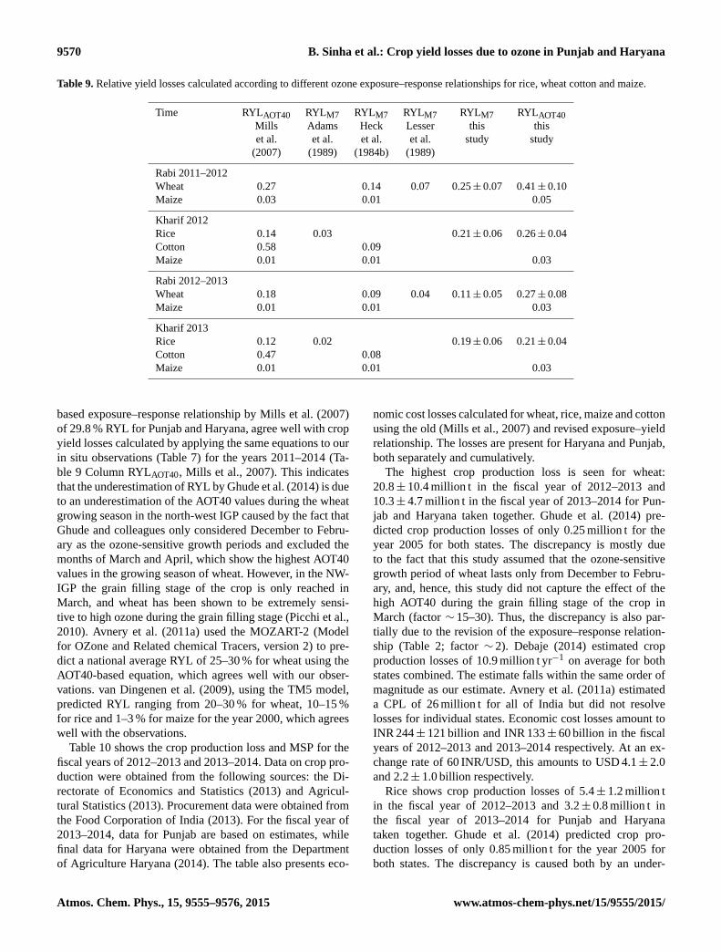
Table 9 summarizes the relative yield loss calculated accord-

ing to different exposure indices. In general, crop production

losses calculated using the M7 index exposure–response rela-

tionships based on American studies conducted in the 1970s

Table 8. Ozone exposure according to different exposure indices

and relative yields for rabi and kharif maize.

Time AOT40 M7 RYAOT40 RYM7 RYAOT40

Mills Heck Indian

et al. et al. OTC

(2007) (1984b)

2012 P1 11 346 46 0.98 0.97 0.95

2012 P2 7522 43 0.99 0.99 0.98

Average 9434 45 0.99 0.99 0.97

2011/2012 P3 9824 48 0.98 0.99 0.96

2011/2012 P4 15 406 56 0.96 0.98 0.93

Average 12 615 52 0.97 0.99 0.95

2013 P1 9496 46 1.00 0.99 0.97

2013 P2 7209 44 0.98 0.99 0.98

Average 8353 45 0.99 0.99 0.97

2012/2013 P3 6219 40 0.99 0.99 0.99

2012/2013 P4 12 455 51 0.99 0.99 0.95

Average 9337 46 0.99 0.99 0.97

and 1980s (Heck et al., 1984b; Adams et al., 1989; Lesser

et al., 1990) tend to underestimate the actual yield losses of

Indian cultivars, as the M7 index fails to capture the effect

of extreme events on plant physiology and yields (Tuovi-

nen, 2000; Hollaway et al., 2012). The old AOT40 exposure–

response relationship by Mills et al. (2007) does not cap-

ture the sensitivity of most southern Asian cultivars. Only

Bangladeshi rice cultivars and a few select wheat cultivars

follow this relationship, while most Indian wheat and rice

cultivars are far more sensitive to elevated ozone levels. We

propose a revised relationship (Table 2, Figs. 4 and 6) based

on a literature review of OTC studies conducted on Indian

cultivars and demonstrate that this relationship adequately

describes the empirical relationship between crop yield and

AOT40 in field trials that were not aimed at studying the ef-

fect of ozone on crops. The revised equation (Table 2) pre-

dicts that RYL for Indian cultivars are 1.5–2 times the RYL

predicted based on the equation by Mills et al. (2007).

A recent modelling study for the year 2005 predicted

RYLs of 1 and 1.2 % for Punjab and Haryana respectively

for wheat and 8.1 % for Punjab for rice (Ghude et al., 2014).

These relative yield losses are a factor of 15–30 lower com-

pared to the RYL calculated using the same equation (Mills

et al., 2007) but employing in situ measurements for calcu-

lating AOT40 for wheat and a factor of 1.5 to 1.8 lower for

rice (Table 9 Column RYLAOT40, Mills et al., 2007).

Debaje (2014) estimated the crop production loss of win-

ter wheat based on a review of measured ozone mixing ratios

published in the peer-reviewed literature for the years 2000–

2007. The calculated relative yield losses, based both on the

M7 exposure–response relationship for winter wheat pro-

posed by Lesser et al. (1990) of 10.8 % and on the AOT40-



Table 9. Relative yield losses calculated according to different ozone exposure–response relationships for rice, wheat cotton and maize.

Time RYLAOT40 RYLM7 RYLM7 RYLM7 RYLM7 RYLAOT40

Mills Adams Heck Lesser this this

et al. et al. et al. et al. study study

(2007) (1989) (1984b) (1989)

Rabi 2011–2012

Wheat 0.27 0.14 0.07 0.25± 0.07 0.41± 0.10

Maize 0.03 0.01 0.05

Kharif 2012

Rice 0.14 0.03 0.21± 0.06 0.26± 0.04

Cotton 0.58 0.09

Maize 0.01 0.01 0.03

Rabi 2012–2013

Wheat 0.18 0.09 0.04 0.11± 0.05 0.27± 0.08

Maize 0.01 0.01 0.03

Kharif 2013

Rice 0.12 0.02 0.19± 0.06 0.21± 0.04

Cotton 0.47 0.08

Maize 0.01 0.01 0.03

based exposure–response relationship by Mills et al. (2007)

of 29.8 % RYL for Punjab and Haryana, agree well with crop

yield losses calculated by applying the same equations to our

in situ observations (Table 7) for the years 2011–2014 (Ta-

ble 9 Column RYLAOT40, Mills et al., 2007). This indicates

that the underestimation of RYL by Ghude et al. (2014) is due

to an underestimation of the AOT40 values during the wheat

growing season in the north-west IGP caused by the fact that

Ghude and colleagues only considered December to Febru-

ary as the ozone-sensitive growth periods and excluded the

months of March and April, which show the highest AOT40

values in the growing season of wheat. However, in the NW-

IGP the grain filling stage of the crop is only reached in

March, and wheat has been shown to be extremely sensi-

tive to high ozone during the grain filling stage (Picchi et al.,

2010). Avnery et al. (2011a) used the MOZART-2 (Model

for OZone and Related chemical Tracers, version 2) to pre-

dict a national average RYL of 25–30 % for wheat using the

AOT40-based equation, which agrees well with our obser-

vations. van Dingenen et al. (2009), using the TM5 model,

predicted RYL ranging from 20–30 % for wheat, 10–15 %

for rice and 1–3 % for maize for the year 2000, which agrees

well with the observations.

Table 10 shows the crop production loss and MSP for the

fiscal years of 2012–2013 and 2013–2014. Data on crop pro-

duction were obtained from the following sources: the Di-

rectorate of Economics and Statistics (2013) and Agricul-

tural Statistics (2013). Procurement data were obtained from

the Food Corporation of India (2013). For the fiscal year of

2013–2014, data for Punjab are based on estimates, while

final data for Haryana were obtained from the Department

of Agriculture Haryana (2014). The table also presents eco-

nomic cost losses calculated for wheat, rice, maize and cotton

using the old (Mills et al., 2007) and revised exposure–yield

relationship. The losses are present for Haryana and Punjab,

both separately and cumulatively.

The highest crop production loss is seen for wheat:

20.8± 10.4 million t in the fiscal year of 2012–2013 and

10.3± 4.7 million t in the fiscal year of 2013–2014 for Pun-

jab and Haryana taken together. Ghude et al. (2014) pre-

dicted crop production losses of only 0.25 million t for the

year 2005 for both states. The discrepancy is mostly due

to the fact that this study assumed that the ozone-sensitive

growth period of wheat lasts only from December to Febru-

ary, and, hence, this study did not capture the effect of the

high AOT40 during the grain filling stage of the crop in

March (factor ∼ 15–30). Thus, the discrepancy is also par-

tially due to the revision of the exposure–response relation-

ship (Table 2; factor ∼ 2). Debaje (2014) estimated crop

production losses of 10.9 million t yr−1 on average for both

states combined. The estimate falls within the same order of

magnitude as our estimate. Avnery et al. (2011a) estimated

a CPL of 26 million t for all of India but did not resolve

losses for individual states. Economic cost losses amount to

INR 244± 121 billion and INR 133± 60 billion in the fiscal

years of 2012–2013 and 2013–2014 respectively. At an ex-

change rate of 60 INR/USD, this amounts to USD 4.1± 2.0

and 2.2± 1.0 billion respectively.

Rice shows crop production losses of 5.4± 1.2 million t

in the fiscal year of 2012–2013 and 3.2± 0.8 million t in

the fiscal year of 2013–2014 for Punjab and Haryana

taken together. Ghude et al. (2014) predicted crop pro-

duction losses of only 0.85 million t for the year 2005 for

both states. The discrepancy is caused both by an under-



Tab

le10.

Cro

pp

rod

uct

ion

(CP

)fo

rP

un

jab

(PB

)an

dH

ary

ana

(HR

)an

dM

SP

for

the

fisc

aly

ears

of

20

12

–2

01

3an

d2

01

3–

20

14

.C

rop

pro

du

ctio

nlo

ss(C

PL

)an

dec

on

om

icco

st

loss

es(E

CL

)ar

eca

lcu

late

dfo

rw

hea

t,ri

ce,m

aize

and

cott

on

usi

ng

the

old

AO

T4

0-b

ased

exp

osu

re–

yie

ldre

lati

on

ship

(Mil

lset

al.,

20

07

)aan

dfo

rw

hea

tan

dri

ce,al

sou

sin

gth

ere

vis

ed

AO

T4

0-b

ased

exp

osu

re–

resp

on

sere

lati

on

ship

b.

CP

and

CP

Lfo

rri

ce,

wh

eat

and

mai

zear

eg

iven

into

nn

es(t

);C

Pan

dC

PL

are

giv

enin

bal

es(b

).

CP

CP

CP

MS

PC

PL

aC

PL

aC

PL

aE

CL

aE

CL

aE

CL

aC

PL

bC

PL

bC

PL

bE

CL

bE

CL

bE

CL

b

PB

HR

To

tal

PB

HR

To

tal

PB

HR

To

tal

PB

HR

To

tal

PB

HR

To

tal

20

12

–1

06

t1

06

t1

06

tIN

R/k

g1

06

t1

06

t1

06

t1

06IN

R1

06IN

R1

06IN

R1

06

t1

06

t1

06

t1

06

INR

10

6IN

R1

06

INR

20

13

Wh

eat

17

.28

12

.69

29

.97

11

.76

.39

4.6

91

1.0

97

47

77

54

91

51

29

69

21

2.0

18

.80

20

.81

14

04

95

10

31

76

24

36

71

Ric

e1

1.3

73

.98

15

.35

12

.51

.85

0.6

52

.50

23

13

78

09

93

12

35

4.0

01

.40

5.3

94

99

36

17

48

06

74

16

Mai

ze0

.48

0.0

20

.50

11

.75

0.0

05

0.0

00

20

.00

55

62

59

0.0

15

0.0

01

0.0

15

17

37

18

0

10

6b

10

6b

10

6b

INR

/b1

06

b1

06

b1

06

b1

06IN

R1

06IN

R1

06IN

R

Co

tto

n2

2.5

4.5

12

73

72

.83

.56

.23

51

79

43

97

47

91

54

20

13

–1

06

t1

06

t1

06

tIN

R/k

g1

06

t1

06

t1

06

t1

06IN

R1

06IN

R1

06IN

R1

06

t1

06

t1

06

t1

06

INR

10

6IN

R1

06

INR

20

14

Wh

eat

16

.11

11

.80

27

.91

12

.85

3.5

42

.44

6.1

34

54

42

33

28

57

87

27

5.9

34

.36

10

.32

76

56

75

60

82

13

26

49

Ric

e8

.16

4.0

01

2.1

61

3.1

1.1

10

.55

1.6

61

45

77

71

42

21

71

92

.17

1.0

63

.23

28

41

51

39

22

42

33

8

Mai

ze0

.56

0.0

30

.60

13

.10

.00

60

.00

03

0.0

06

74

47

80

.01

70

.00

10

.01

82

28

11

23

9

10

6b

10

6b

10

6b

INR

/b

10

6b

10

6b

10

6b

10

6IN

R1

06IN

R1

06IN

R

Co

tto

n2

.12

.04

.11

30

64

1.9

1.8

3.6

24

32

92

31

70

47

49

9



estimation of the AOT40 due to the fact that the author

considered a shorter ozone-sensitive growth period (fac-

tor 1.5–1.8) and by the revision of the exposure–yield re-

lationship (Table 2) to account for the sensitivity of In-

dian rice cultivars (factor 1.9). Economic losses amount

to INR 67± 15 billion and INR 42± 11 billion for the fiscal

years of 2012–2013 and 2013–2014 respectively. At an ex-

change rate of 60 INR/USD, this amounts to USD 1.1± 0.2

and 0.7± 0.2 billion respectively.

The Indian National Food Security Ordinance entitles

∼ 820 million of India’s poor to purchase about 60 kg of rice

or wheat per person annually at subsidized rates. The scheme

requires 27.6 Mt of wheat and 33.6 Mt of rice per year. Cut-

ting down ozone-related crop production losses in Punjab

and Haryana alone could provide > 50 % of the wheat and

10 % of the rice required for the scheme.

Economic losses amount to INR 79.15 billion and

47.50 billion (USD 1.3 and 0.8 billion) for cotton and

INR 0.18 billion and INR 0.24 billion (USD 3 and 4 million)

for maize in the fiscal years of 2012–2013 and 2013–2014

respectively.

The total economic losses for the agricultural sector

in Punjab and Haryana amount to INR 391± 136 billion

(USD 6.5± 2.2 billion) in the fiscal year of 2012–2013

and INR 223± 71 billion (USD 3.7± 1.2 billion) in the fiscal

year of 2013–2014. The loss estimates presented above un-

derestimate the real economic losses due to ozone on several

accounts.

Firstly, the crop is valued only at the MSP for common

grade crops. The MSP is often even lower than the actual

production cost and the economic value of the crop is typi-

cally much higher. This is particularly true for high-quality

rice varieties such as basmati.

Secondly, we do not account for the losses in the food

processing sector and other allied industries. The value gain

from MSP to the final end consumer product ranges from a

factor of 2 to 20 for food crops to a factor of > 100 for cotton.

Thirdly, this calculation does not consider the relationship

between the rural demand for consumer products and rural

income. Rural income is affected strongly by crop yields,

78 % of the rural population depends on agriculture as pri-

mary source of income.

Previous studies investigating the relationship between

monsoon rainfall, food grain production and the nation’s

GDP for the years 1951–2003 (Gadgil and Gadgil, 2006)

found that a 1 % decrease in food grain production due to

a deficient monsoon led to a 0.36 % decrease in India’s GDP.

Ozone-related crop production losses are likely subject to the

same multiplication factor. With relative yields losses cur-

rently ranging from 10 to 58 % for the different crops (Avn-

ery et al. (2011a), van Dingenen et al., 2009), the real eco-

nomic burden of current ozone levels in terms of India’s GDP

is likely to fall into the range from 3.6 to 20 % (Eq. 8).

4 Conclusions

Using a high-quality data set of in situ ozone measurements

in the NW-IGP and yield data from the two neighbouring

states of Punjab and Haryana, we derived a new crop-yield–

ozone-exposure relationship for Indian rice and wheat culti-

vars. Indian cultivars are a factor of 2–3 more sensitive to

ozone than to their European and south-east Asian coun-

terparts. Relative yield losses based on the AOT40 metrics

ranged from 30–42 % for wheat, 22–26 % for rice, 3–5 % for

maize to 47–58 % for cotton.

Crop production losses for wheat amounted to

20.8± 10.4 million t in the fiscal year of 2012–2013

and 10.3± 4.7 million t in the fiscal year of 2013–2014

for Punjab and Haryana taken together. Crop production

losses for rice totaled 5.4± 1.2 million t in the fiscal year

of 2012–2013 and 3.2± 0.8 million t in the year 2013–2014

for Punjab and Haryana taken together. Cutting these

ozone-related crop production losses alone could provide

50 % of the wheat and 10 % of the rice required to provide

60 kg of subsidized wheat or rice to ∼ 820 million of India’s

economically weaker members of society.

The lower limit for economic cost losses in Punjab and

Haryana amounted to USD 6.5± 2.2 billion in the fiscal year

of 2012–2013 and USD 3.7± 1.2 billion in the fiscal year

of 2013–2014. The upper limit for the ozone-related eco-

nomic losses incurred at current ozone levels for all of India

amounts to 3.5–20 % of India’s GDP. The wealth gained by

mitigating tropospheric ozone and decreasing ozone-related

economic losses would be distributed among a large group

of beneficiaries, as 54 % of the India’s population and 79 %

of India’s rural population still rely on agriculture as their

principle source of income. Co-benefits of ozone mitigation

include a decrease in the ozone-related mortality and morbid-

ity, a reduction in healthcare-related costs and the number of

workdays lost and a reduction in the ozone-induced warming

in the lower troposphere.

At current tropospheric ozone levels, optimizing the sow-

ing date of rice towards sowing at the start of June and trans-

plantation in the first week of July can increase crop yields

substantially by reducing the ozone exposure of the crop.

Reaching out to farmers in order to promote this change in

cropping practice will yield co-benefits in terms of increas-

ing the water productivity of the crop and preserving pre-

cious groundwater. It will also increase the profit margin, as

farmers often run tube wells on diesel whenever grid power

supply is not available.

For wheat, too, timely sowing is crucial to minimize ozone

exposure during the grain filling stage of the crop by ad-

vancing the harvest from the normal time (end of April

to beginning of May) to an earlier time window (end of

March to early April). New tillage practices that facilitate

timely sowing, such as relay seeding into cotton and zero

or low tillage regimes that incorporate rice straw, are ur-

gently required to facilitate timely sowings. Providing a



“Happy Seeder” machine to every village in Punjab would

cost∼USD 0.04 billion. The Happy Seeder sows through the

crop residue and leaves it as mulch on the fields. Promoting

this technology would not only reduce ambient ozone mixing

ratios by curbing crop residue burning, which contributes sig-

nificantly to ozone precursor emission in the post-monsoon

season (Sarkar et al., 2013), but it would also protect the

young seedlings against ozone as the mulch acts as protec-

tive cover and reduces the dry deposition of ozone onto the

leaf surface. Co-benefits of this technology include a higher

carbon sequestration in the soil and a higher water produc-

tivity of the crop.

For all crops, screening a large number of domestic culti-

vars using the new stomatal-flux-based exposure metrics to

identify and promote those cultivars that are less susceptible

to ozone damage also offers a way forward.

The Supplement related to this article is available online

at doi:10.5194/acp-15-9555-2015-supplement.

Acknowledgements. We thank the IISER Mohali Atmospheric

Chemistry Facility for data and the Ministry of Human Resource

Development (MHRD), India, and IISER Mohali for funding the

facility. Yash Maurya and Vinod Kumar gratefully acknowledge

a DST Inspire fellowship, Prafulla Chandra acknowledges a

CSIR-JRF fellowship and Kartikeya Singh Sangwan gratefully

acknowledges the IISER Mohali summer research fellowship

program. We thank the ESA GlobCover 2009 Project (ESA 2010

and UC Louvain) for providing a high-resolution land classification

map of the region. We gratefully acknowledge two anonymous

reviewers, in particular the third anonymous reviewer, whose

valuable comments have added much depth to the discussion in this

paper.

Edited by: T. Butler

References

Adams, R. M., Glyer, J. D., Johnson, S. L., and McCarl, B. A.:

Assessment of the economic effects of ozone on United States

agriculture, JAPCA J. Air Waste Ma., 39, 960–968, 1989.

Agrawal, M., Singh, B., Rajput, M., Marshall, F., and Bell, J. N. B.:

Effect of air pollution on peri-urban agriculture: a case study,

Environ. Pollut., 126, 323–329, 2003.

Agricultural Statistics: Government of India, Ministry of Agricul-

ture, Department of Agriculture and Cooperation, Directorate of

Economics and Statistics, Pocket Book on Agricultural Statistics

2013, New Delhi, 2013.

Ainsworth, E. A., Yendrek, C. R., Sitch, S., Collins, W. J., and

Emberson, L. D.: The effects of tropospheric ozone on net pri-

mary productivity and implications for climate change, Ann.

Rev. Plant Biol., 63, 637–661, 2012.

Akhtar, N., Yamaguchi, M., Inada, H., Hoshino, D., and Kondo, T.:

Effects of ozone on growth, yield and leaf gas exchange rates

of four Bangladeshi cultivars of rice (Oryza sativa L.), Environ.

Pollut., 158, 2970–2973, 2010a.

Akhtar, N., Yamaguchi, M., Inada, H., Hoshino, D., Kondo, T., and

Izuta, T.: Effects of ozone on growth, yield and leaf gas ex-

change rates of two Bangladeshi cultivars of wheat (Triticum aes-

tivum L.), Environ. Pollut., 158, 1763–1767, 2010b.

Amin, N., Ken, Y., Toshimasa, O., Junichi, K., and Kazuyo, Y.:

Evaluation of the Effect of Surface Ozone on Main Crops in East

Asia: 2000, 2005, and 2020, Water Air Soil Pollut., 224, 1537,

doi:10.1007/s11270-013-1537-x, 2013.

Avnery, S., Mauzerall, D. L., Liu, J., and Horowitz, L. W.: Global

crop yield reductions due to surface ozone exposure 1: Year 2000

crop production losses and economic damage, Atmos. Environ.,

45, 2284–2296, 2011a.

Avnery, S., Mauzerall, D. L., Liu, J., and Horowitz, L. W.: Global

crop yield reductions due to surface ozone exposure 2: year 2030

potential crop production losses and economic damage under

two scenarios of O3 pollution, Atmos. Environ., 45, 2297–2309,

2011b.

Black, V. J., Black, C. R., Roberts, J. A., and Stewart, C. A.: Impact

of ozone on the reproductive development of plants, New Phytol.,

147, 421–447, 2000.

Brar, S. K., Mahal, S. S., Brar, A. S., Vashist, K. K., Sharma, N.,

and Buttar, G. S.: Transplanting time and seedling age affect wa-

ter productivity, rice yield and quality in north-west India, Agr.

Water Manage., 115, 217–222, 2012.

Buttar, G. S., Sidhu, H. S., Singh, V., Jats, M.L, Gupta, R., Singh, Y.,

and Singh, B.: Relay planting of wheat in cotton: an innovative

technology for enhancing productivity and profitability of wheat

in cotton-wheat production systems of South Asia, Exp. Agr., 49,

19–30, 2013.

Calatayud, A., Iglesias, D., Talon, M., and Barreno, E.: Response

of spinach leaves (spinacia oleracea I.) to ozone measured by gas

exchange, chlorophyll a fuorescence, antioxidant systems, and

lipid peroxidation, Photosynthetica, 42, 23–29, 2004.

Census: Government of India, Ministry of Home Affairs, Office of

the Registrar General and Census Commissioner, India, avail-

able at: http://www.censusindia.gov.in/pca/default.aspx (last ac-

cess: 6 June 2014), 2011.

Chahal, G. B. S., Sood, A., Jalota, S. K., Choudhury, B. U., and

Sharma, P. K.: Yield, evapotranspiration and water productivity

of rice (Oryza sativa L.) and wheat (Triticum aestivum L.) system

in Punjab (India) as influenced by transplanting date of rice and

weather parameters, Agr. Water Manage., 88, 14–22, 2007.

Chuwah, C., van Noije, T., van Vuuren, D. P., Stehfest, E., and

Hazeleger, W.: Global impacts of surface ozone changes on crop

yields and land use, Atmos. Environ., 106, 11–23, 2015.

Coventry, D. R., Gupta, R. K., Yadav, A., Poswal, R. S.,

Chhokar, R. S., Sharma, R. K., Yadav, V. K., Gill, S. C., Ku-

mar, A., Metha, A., Kleeman, S. G. L., Bonamanof, A., and Cum-

min, J. A.: Wheat quality and productivity as affected by varieties

and sowing time in Haryana, India, Field Crop. Res., 123, 214–

225, 2011.

Danielsson, H., Karlsson, P. E., and Pleijel, H.: An ozone response

relationship for four Phleum pratense genotypes based on mod-

elling of the phytotoxic ozone dose (POD), Environ. Exp. Bot.,

90, 70–77, 2013.

Das, P. K.: Mean vertical motion and non-adiabatic heat sources

over India during the monsoon, Tellus, 14, 212–220, 1962.


http://dx.doi.org/10.5194/acp-15-9555-2015-supplement

http://dx.doi.org/10.1007/s11270-013-1537-x

http://www.censusindia.gov.in/pca/default.aspx


Debaje, P. K.: Estimated crop yield losses due to surface ozone

exposure and economic damages in India, Environ. Sci. Pollut.

Res., 21, 7329–7338, 2014.

Deb Roy, S., Beig, G., and Ghude, S. D.: Exposure-plant response

of ambient ozone over the tropical Indian region, Atmos. Chem.

Phys., 9, 5253–5260, doi:10.5194/acp-9-5253-2009, 2009.

Department of Agriculture Haryana: Rabi crop production ,

available at: http://www.agriharyana.nic.in/Stat_Info/Final_

Estimates_Rabi_2013-14.pdf, last access: 21 September 2014

and kharif crop production, available at: http://www.agriharyana.

nic.in/Stat_Info/Final_estimates_2013-2014.doc, last access:

21 September 2014.

Directorate of Economics and Statistics: Department of Agricul-

ture and Cooperation, Agricultural Statistics At a Glance 2013,

available at: http://eands.dacnet.nic.in/latest_2013.htm (last ac-

cess: 18 September 2014), 2013.

Emberson, L. D., Ashmore, M. R., Cambridge, H. M., Simpson, D.,

and Tuovinen, J.-P.: Modelling stomatal ozone flux across Eu-

rope, Environ. Pollut. 109, 403–413, 2000.

Emberson, L. D., Buker, P., Ashmore, M., Mills, G., Jackson, L.,

Agrawal, M., Atikuzzaman, M., Cinderby, S., Engardt, M.,

Jamir, C., Kobayashi, K., Oanh, N., Quadir, Q., and Wahid, A.:

A comparison of North-American and Asian exposure-response

data for ozone effects on crop yields, Atmos. Environ., 43, 1945–

1953, 2009.

FAO – Food and Agriculture Organization of the United Nations:

Statistical Yearbook 2013, Rome, 2013.

Fares, S., Matteucci, G., Scarascia Mugnozza, G., Morani, A., Cal-

fapietra, C., Salvatori, E., Fusaro, L., Manes, F., and Loreto, F.:

Testing of models of stomatal ozone fluxes with field measure-

ments in a mixed Mediterranean forest, Atmos. Environ., 67,

242–251, 2013.

Feng, Z., Tang, H., Uddling, J., Pleijel, H., Kobayashi, K., Zhu, J.,

Oue, H., and Guo, W.: A stomatal ozone fluxeresponse relation-

ship to assess ozone-induced yield loss of winter wheat in sub-

tropical China, Environ. Pollut., 164, 16–23, 2012.

Feng, Z., Hu, E., Wang, X., Jiang, L., and Liu, X.: Ground-level

O3 pollution and its impacts on food crops in China: A review,

Environ. Pollut., 199, 42–45, 2015.

Food Corporation of India 2013, available at: http://fciweb.nic.in/

procurements/view/43 (last access: 21 September 2014), 2013.

Fuhrer, J., Skärby, L., and Ashmore, M.: Critical levels for ozone ef-

fects on vegetation in Europe, Environ. Pollut., 97, 91–106, 1997.

Gadgil, S. and Gadgil, S.: The Indian monsoon, GDP and agricul-

ture, Econ. Polit. Weekly, 41, 4889–4895, 2006.

Ghude, S. D., Jain, S. L., Arya, B. C., Beig, G., Ahammed, Y. N.,

Kumar, A., and Tyagi, B.: Ozone in ambient air at a tropical

megacity, Delhi: characteristics, trends and cumulative ozone ex-

posure indices, J. Atmos. Chem., 60, 237–252, 2008.

Ghude, S. D., Jena, C., Chate, D. M., Beig, G., Pfis-

ter, G. G., Kumar, R., and Ramanathan, V.: Reduction in In-

dias crop yield due to ozone, Geophys. Res. Lett., 41, 51971,

doi:10.1002/2014GL060930, 2014.

Giles, J.: Hikes in surface ozone could suffocate crops, Nature, 435,

7, doi:10.1038/435007a, 2005.

Gonzalez-Fernandez, I., Bermejo, V., Elvira, S., de la Torre, D.,

Gonzalez, A., Navarrete, L., Sanz, J., Calvete, H., Garcia-

Gomez, H., Lopez, A., Serra, J., Lafarga, A., Armesto, A. P.,

Calvo, A., and Alonso, R.: Modelling ozone stomatal flux of

wheat under mediterranean conditions, Atmos. Environ., 67,

149–160, 2013.

Haagen-Smit, A. J.: Chemistry and Physiology of Los Angeles

smog, Ind. Eng. Chem., 44, 1342–1346, 1952.

Haagen-Smit, A. J. and Fox, M. M.: Photochemical ozone forma-

tion with hydrocarbons and automobile exhaust, JAPCA J. Air

Waste Ma., 4, 105–109, 1954.

Heath, R. L.: Modification of the biochemical pathways of plants

induced by ozone: What are the varied routes to change?, Envi-

ron. Pollut., 155, 453–463, 2008.

Heck, W. W., Cure, W. W., Rawlings, J. O., Zaragoza, L. J., Hea-

gle, A. S., Heggestad, H. E., Kohut, R. J., Kress, L. W., and

Temple, P. J.: Assessing impacts of ozone on agricultural crops:

I: Overview, JAPCA J. Air Waste Ma., 34, 729–735, 1984a.

Heck, W. W., Cure, W. W., Rawlings, J. O., Zaragoza, L. J.,

Heagle, A. S., Heggestad, H. E., Kohut, R. J., Kress, L. W.,

and Temple, P. J.: Assessing impacts of ozone on agricultural

crops: II: Crop yield functions and alternative exposure statistics,

JAPCA J. Air Waste Ma., 34, 729–735, 1984b.

Hollaway, M. J., Arnold, S. R., Challinor, A. J., and Ember-

son, L. D.: Intercontinental trans-boundary contributions to

ozone-induced crop yield losses in the Northern Hemisphere,

Biogeosciences, 9, 271–292, doi:10.5194/bg-9-271-2012, 2012.

Iriti, M. and Faoro, F.: Chemical diversity and defence metabolism:

How plants cope with pathogens and ozone pollution, Int. J.

Molec. Sci., 10, 3371–3399, 2009.

Jain, S. L., Arya, B. C., and Kumar, A.: Observational study of sur-

face ozone at New Delhi, India, Int. J. Remote Sens., 26, 3515–

3526, 2005.

Jalota, S. K., Buttar, G. S., Sood, A., Chahal, G. B. S., Ray, S. S., and

Panigrahy, S.: Effects of sowing date, tillage and residue man-

agement on productivity of cotton (Gossypium hirsutum L.), Soil

Till. Res., 99, 76–83, 2008.

Jalota, S. K., Singh, K. B., Chahal, G. B. S., Gupta, R. K.,

Chakraborty, S., Sood, A., Ray, S. S., and Panigrahy, S.: In-

tegrated effect of transplanting date, cultivar and irrigation

on yield, water saving and water productivity of rice (Oryza

sativa L.) in Indian Punjab: field and simulation study, Agr. Wa-

ter Manage., 96, 1096–1104, 2009.

Kangasjaärvi, J., Jaspers, P., and Kollist, H.: Signalling and cell

death in ozone-exposed plants, Plant Cell Environ., 28, 1021–

1036, 2005.

Kangasjaärvi, S. and Kangasjaärvi, J.: Towards Understanding Ex-

tracellular ROS Sensory and Signaling Systems in Plants, Advan.

Bot., 28, 538946, doi:10.1155/2014/538946, 2014.

Kumar, R., Naja, M., Venkataramani, S., and Wild, O.: Vari-

ations in surface ozone at Nainital: a high–altitude site

in the central Himalayas, J. Geophys. Res., 115, D16302,

doi:10.1029/2009JD013715, 2010.

Lal, D. M., Ghude, S. D., Patil, S. D., Kulkarni, S. H., Jena, C., Ti-

wari, S., and Srivastava, M. K.: Tropospheric ozone and aerosol

long-term trends over the Indo-Gangetic Plain (IGP), India, At-

mos. Res., 116, 82–92, 2012.

Lee, E. H. and Hogsett, W. E.: Role of concentration and time of day

in developing ozone exposure indices for a secondary standard, J.

Air Waste Manage., 49, 669–681, 1999.

Lefohn, A. S., Laurence, J. A., and Kohut, R. J.: A comparison of

indices that describe the relationship between exposure to ozone


http://dx.doi.org/10.5194/acp-9-5253-2009

http://www.agriharyana.nic.in/Stat_Info/Final_Estimates_Rabi_2013-14.pdf

http://www.agriharyana.nic.in/Stat_Info/Final_Estimates_Rabi_2013-14.pdf

http://www.agriharyana.nic.in/Stat_Info/Final_estimates_2013-2014.doc

http://www.agriharyana.nic.in/Stat_Info/Final_estimates_2013-2014.doc

http://eands.dacnet.nic.in/latest_2013.htm

http://fciweb.nic.in/procurements/view/43

http://fciweb.nic.in/procurements/view/43

http://dx.doi.org/10.1002/2014GL060930

http://dx.doi.org/10.1038/435007a

http://dx.doi.org/10.5194/bg-9-271-2012

http://dx.doi.org/10.1155/2014/538946

http://dx.doi.org/10.1029/2009JD013715


and reduction in the yield of agricultural crops, Atmos. Res., 22,

1229–1240, 1988.

Leisner, C. P. and Ainsworth, E. A.: Quantifying the effects of ozone

on plant reproductive growth and development, Global Change

Biol., 18, 606–616, 2012.

Lesser, V. M., Rawlings, J. O., Spruill, S. E., and Somerville, M. C.:

Ozone effects on agricultural crops: statistical methodologies and

estimated dose–response relationships, Crop Sci., 30, 148–155,

1990.

Maggs, R. and Ashmore, M. R.: Rowth and yield responses of Pak-

istan rice (Oryza sativa L.) cultivars to O3 and NO2, Environ.

Pollut., 103, 159–170, 1998.

Maggs, R., Wahid, A., Shamsi, S. R. A., and Ashmore, M. R.: Ef-

fects of ambient air pollution on wheat and rice yield in Pakistan,

Air Soil Pollut., 85, 1311–1316, 1995.

Mahajan, G., Bharaj, T. S., and Timsina, J.: Yield and water pro-

ductivity of rice as affected by time of transplanting in Punjab,

India, Agr. Water Manage., 96, 525–532, 2009.

Mauzerall, D. L. and Wang, X.: Protecting agricultural crops from

the effects of tropospheric ozone exposure: reconciling science

and standard setting in the United States, Europe, and Asia,

Annu. Rev. Energ. Env., 26, 237–268, 2001.

Mills, G., Buse, A., Gimeno, B., Bermejo, V., Holland, M., Ember-

son, L., and Pleijel, H.: A synthesis of AOT40-based response

functions and critical levels for ozone for agricultural and horti-

cultural crops, Atmos. Environ., 41, 2630–2643, 2007.

Mills, G., Hayes, F., Simpson, D., Emberson, L., Norris, D., Har-

mens, H., and Buüker P.: Evidence of widespread effects of

ozone on crops and semi–natural vegetation in Europe (1990–

2006) in relation to AOT40 – and flux–based risk maps, Glob.

Change Biol., 17, 592–613, 2011a.

Mills, G., Pleijel, H., Braun, S., Büker P., Bermejo, V., Calvo, E.,

Danielsson, H., Emberson, L., Gonzalez Fernandez, I., Grün-

hage L., Harmens, H., Hayes, F., Karlsson, P.-E., and Simp-

son, D.: New stomatal flux-based critical levels for ozone effects

on vegetation, Atmos. Environ., 45, 5064–5068, 2011b.

Mittal, M. L., Hess, P. G., Jain, S. L., Arya, B. C., and Sharma, C.:

Surface ozone in the Indian region, Atmos. Environ., 41, 6572–

6584, 2007.

Oksanen, E., Pandey, V., Pandey, A., Keski-Saari, S., Kontunen-

Soppela, S., and Sharma, C.: Impacts of increasing ozone on In-

dian plants, Environ. Pollut., 177, 189–200, 2013.

Panigrahy, S., Upadhyay, G., Ray, S. S., and Parihar, J. S.: Mapping

of cropping system for the Indo-Gangetic plain using multi-date

SPOT NDVI-VGT data, J. Indian Soc. Remote Sens., 38, 627–

632, 2010.

Pawar, H., Garg, S., Kumar, V., Sachan, H., Arya, R., Sarkar, C.,

Chandra, B. P., and Sinha, B.: Quantifying the contribution of

long-range transport to Particulate Matter (PM) mass loadings at

a suburban site in the North-Western Indo Gangetic Plain (IGP),

Atmos. Chem. Phys., 15, 9501–9520, doi:10.5194/acp-15-9501-

2015, 2015.

Picchi, V., Iritia, M., Quaroni, S., Saracchic, M., Viola, P., and

Faoro, F.: Climate variations and phenological stages modu-

late ozone damages in field-grown wheat, A three-year study

with eight modern cultivars in Po Valley (Northern Italy), Agr.

Ecosyst. Environ., 135, 310–317, 2010.

Pleijel, H., Skärby, L., Wallin, G., and Sellden, G.: Yield and grain

quality of spring wheat (triticum aestivum l., cv. drabant) ex-

posed to different concentrations of ozone in open–top chambers,

Agr. Environ. Pollut., 69, 151–168, 1991.

Rai, R. and Agrawal, M.: Evaluation of physiological and biochem-

ical responses of two rice (Oryza sativa L.) cultivars to ambient

air pollution using open top chambers at a rural site in India, Sci.

Total Environ., 407, 679–691, 2008.

Rai, R., Agrawal, M., and Agrawal, S. B.: Assessment of yield

losses in tropical wheat using open top chambers, Agriculture,

Environ. Pollut., 41, 9543–9554, 2007.

Rai, R., Agrawal, M., and Agrawal, S. B.: Threat to food security

under current levels of ground level ozone: a case study for In-

dian cultivars of rice, Atmos. Environ., 44, 4272–4282, 2010.

Ram, H., Dadhwal, V., Vashist, K. K., and Kaur, H.: Grain yield and

water use efficiency of wheat (Triticum aestivum L.) in relation

to irrigation levels and rice straw mulching in North West India,

Agr. Water Manage., 128, 92–101, 2013.

RBI – Reserve Bank of India: Handbook of Indian Statistics 2012–

2013, available at: http://rbidocs.rbi.org.in/rdocs/Publications/

PDFs/FHB160913FLS.pdf (last access: 6 June 2014), 2013.

Sarkar, A. and Agrawal, S. B.: Elevated ozone and two modern

wheat cultivars: An assessment of dose dependent sensitivity

with respect to growth, reproductive and yield parameters, En-

viron. Exp. Bot., 69, 328–337, 2010.

Sarkar, A. and Agrawal, S. B.: Evaluating the response of two high

yielding Indian rice cultivars against ambient and elevated levels

of ozone by using open top chambers, J. Environ. Manage., 95,

19–24, 2012.

Sarkar, C., Kumar, V., and Sinha, V.: Massive emissions of carcino-

genic benzenoids from paddy residue burning in North India,

Curr. Sci. India, 104, 1703–1706, 2013.

Satsangi, G. S., Lakhani, A., Kulshrestha, P. R., and Taneja, A.:

Seasonal and diurnal variation of surface ozone and a preliminary

analysis of exceedance of its critical levels at a semi-arid site in

India, J. Atmos. Chem., 47, 271–286, 2004.

Sawada, H. and Kohno, Y.: Differential ozone sensitivity of rice cul-

tivars as indicated by visible injury and grain yield, Plant Biol.,

11, 70–75, 2009.

Sawada, H., Komatsu, S., Nanjo, Y., Khan, N. A., and Kohno, Y.:

Proteomic analysis of rice response involved in reduction of grain

yield under elevated ozone stress, India, Environ. Exp. Bot., 77,

108–116, 2012.

Sharma, P., Kuniyal, J. C., Chand, K., Guleria, R. P., Dhyani, P. P.,

and Chauhan, C.: Surface ozone concentration and its behaviour

with aerosols in the northwestern Himalaya, India, Atmos. Envi-

ron., 71, 44–53, 2004.

Sharma, P. K. and Sood, A.: Remote sensing and GIS techniques in

agricultural development? A case study of Punjab, J. Agr. Phys.,

3, 174–181, 2003.

Singh, A. A., Agrawal, S. B., Shahi, J. P., and Agrawal, M.: As-

sessment of growth and yield losses in two Zea mays L. cultivars

(quality protein maize and nonquality protein maize) nder pro-

jected levels of ozone, Environ. Sci. Pollut. Res., 21, 2628–2641,

2014.

Singh, S. and Agrawal, M.: Impact of tropospheric ozone on wheat

(Triticum aestivum L.) in the eastern Gangetic plains of India as

assessed by ethylenediurea (EDU) application during different

developmental stages, Ecosyst. Environ., 138, 214–221, 2010.

Singh, S., Agrawal, S. B., and Agrawal, M.: Use of ethylene di-

urea (EDU) in assessing the impact of ozone on growth and pro-




http://rbidocs.rbi.org.in/rdocs/Publications/PDFs/FHB160913FLS.pdf

http://rbidocs.rbi.org.in/rdocs/Publications/PDFs/FHB160913FLS.pdf


ductivity of five cultivars of Indian wheat (Triticum aestivum L.),

Environ. Monit. Assess., 159, 125–141, 2009.

Singla, V., Satsangi, A., Pachauri, T., Lakhani, A., and Ku-

mari, K. M.: Ozone formation and destruction at a sub-urban

site in North Central region of India, Atmos. Res., 101, 373–385,

2011.

Sinha, V., Kumar, V., and Sarkar, C.: Chemical composition of pre-

monsoon air in the Indo-Gangetic Plain measured using a new

air quality facility and PTR-MS: high surface ozone and strong

influence of biomass burning, Atmos. Chem. Phys., 14, 5921–

5941, doi:10.5194/acp-14-5921-2014, 2014.

Teixeira, E., Fischer, G., van Velthuizen, H., van Dingenen, R., Den-

tener, F., Mills, G., Walter, C., and Ewert, F.: Limited potential of

crop management for mitigating surface ozone impacts on global

food supply, Atmos. Environ., 45, 2569–2576, 2011.

Tiwari, S., Rai, R., and Agrawal, M.: Annual and seasonal variations

in tropospheric ozone concentrations around Varanasi, Int. J. Re-

mote Sens., 29, 4499–4514, 2008.

Tong, D. Q., Mathur, R., Kang, D. W., Yu, S. C., Schere, K. L., and

Pouliot, G.: Vegetation exposure to ozone over the continental

United States: Assessment of exposure indices by the Eta-CMAQ

air quality forecast model, Atmos. Environ., 43, 724–733, 2009.

Torsethaugen, G., Pell, E. J., and Assmann, S. M.: Ozone inhibits

guard cell K+ channels implicated in stomatal opening, P. Natl.

Acad. Sci. USA, 96, 13577–13582, 1999.

Tuovinen, J. P.: Assessing vegetation exposure to ozone: properties

of the AOT40 index and modiffcations by deposition modelling,

Environ. Pollut., 109, 361–372, 2000.

Turmel, M. S., Espinosa, J. Franco, L., Perez, C., Hernandez, H.,

Gonzalez, E., Fernandez, G., Rojas, C., Sanchez, D., Fernan-

dez, N., Barrios, M., Whalen, J. K., and Turner, B. L.: On-farm

evaluation of a low-input rice production system in Panama,

Paddy Water Environ., 9, 155–161, 2011.

UNECE – United Nations Economic Commission for Europe:

Manual in Methodologies and Criteria for Modelling and Map-

ping Critical Loads and Levels and Air Pollution Effects, Risks

and Trends, in: Chapter 3, Mapping Critical Levels for Veg-

etation, Convention on Long-range Transboundary Air Pollu-

tion, available online at: http://www.icpmapping.org/Mapping_

Manual (last access: 24 June 2015), 2010.

Van Dingenen, R., Dentener, F. J., Raes, F., Krol, M. C., Ember-

son, L., and Cofala, J.: The global impact of ozone on agricul-

tural crop yields under current and future air quality legislation,

Atmos. Environ., 43, 604–618, 2009.

Wahid, A.: Influence of atmospheric pollutants on agriculture in de-

veloping countries: a case study with three new wheat varieties

in Pakistan, Sci. Total Environ., 371, 304–313, 2006.

Wahid, A., Maggs, R., Shamsi, S. R. A., Bell, J. N. B., and Ash-

more, M. R.: Air pollution and its impact on wheat yield in the

Pakistan Punjab, Environ. Pollut., 88, 147–154, 1995a.

Wahid, A., Maggs, R., Shamsi, S. R. A., Bell, J. N. B., and Ash-

more, M. R.: Effects of air pollution on rice yield in the Pakistan

Punjab, Environ. Pollut., 90, 323–329, 1995b.

Wahid, A., Ahmad, S. S., Butt, Z. A., and Ahmad, A. M.: Ex-

ploring the hidden tread of gaseous pollutants using rice (Oryza

sativa L.) plants in Pakistan, Pak. J. Bot., 43, 365–382, 2011.

Wang, X. and Mauzerall, D. L.: Characterizing distributions of sur-

face ozone and its impact on grain production in China, Japan

and South Korea: 1990 and 2020, Atmos. Environ., 38, 4383–

4402, 2004.

Wilkinson, S., Mills, G., Illidge, R., and Davies, W. J.: How is ozone

pollution reducing our food supply?, J. Exp. Bot., 63, 527–536,

doi:10.1093/jxb/err317, 2012.

Yamaguchi, M., Hoshino, D., Inada, H., Akhtar, N., Sumioka, C.,

Takeda, K., and Izuta, T.: Evaluation of the effects of ozone on

yield of Japanese rice (Oryza sativa L.) based on stomatal ozone

uptake, Environ. Pollut., 184, 472–480, 2014.



http://www.icpmapping.org/Mapping_Manual

http://www.icpmapping.org/Mapping_Manual

http://dx.doi.org/10.1093/jxb/err317

assessment of crop yield losses in punjab and haryana using 2

Documents