assessment of data assimilation approaches for the ... vinodkumar et al. vorticity. heat and...

Boundary-Layer Meteorol (2009) 133:343–366DOI 10.1007/s10546-009-9426-y

ARTICLE

Assessment of Data Assimilation Approachesfor the Simulation of a Monsoon Depression Overthe Indian Monsoon Region

Vinodkumar · A. Chandrasekar · K. Alapaty ·Dev Niyogi

Received: 9 December 2008 / Accepted: 31 August 2009 / Published online: 1 October 2009© Springer Science+Business Media B.V. 2009

Abstract A low pressure system that formed on 21 September 2006 over easternIndia/Bay of Bengal intensified into a monsoon depression resulting in copious rainfall overnorth-eastern and central parts of India. Four numerical experiments are performed to exam-ine the performance of assimilation schemes in simulating this monsoon depression usingthe Fifth Generation Mesoscale Model (MM5). Forecasts from a base simulation (with nodata assimilation), a four-dimensional data assimilation (FDDA) system, a simple surfacedata assimilation (SDA) system coupled with FDDA, and a flux-adjusting SDA system(FASDAS) coupled with FDDA are compared with each other and with observations. Themodel is initialized with Global Forecast System (GFS) forecast fields starting from 19 Sep-tember 2006, with assimilation being done for the first 24 hours using conventional obser-vations, sounding and surface data of temperature and moisture from Advanced TIROSOperational Vertical Sounder satellite and surface wind data over the ocean from QuikSCAT.Forecasts are then made from these assimilated states. In general, results indicate that theFASDAS forecast provides more realistic prognostic fields as compared to the other threeforecasts. When compared with other forecasts, results indicate that the FASDAS forecastyielded lower root-mean-square (r.m.s.) errors for the pressure field and improved simulationsof surface/near-surface temperature, moisture, sensible and latent heat fluxes, and potential

Vinodkumar · A. Chandrasekar (B)Department of Physics and Meteorology, Indian Institute of Technology, Kharagpur,West Bengal 721 302, Indiae-mail: [email protected]; [email protected]

Present Address:A. ChandrasekarIndian Institute of Space Science and Technology, Department of Space, Government of India,Thiruvananthapuram 695 022, India

K. AlapatyOffice of Biological and Environmental Research, Office of Science, Department of Energy,Germantown, MD 20874, USA

D. NiyogiDepartment of Agronomy and Department of Earth and Atmospheric Sciences, Purdue University,West Lafayette, IN, USA

123

344 Vinodkumar et al.

vorticity. Heat and moisture budget analyses to assess the simulation of convection revealedthat the two forecasts with the surface data assimilation (SDA and FASDAS) are superiorto the base and FDDA forecasts. An important conclusion is that, even though monsoondepressions are large synoptic systems, mesoscale features including rainfall are affected bysurface processes. Enhanced representation of land-surface processes provides a significantimprovement in the model performance even under active monsoon conditions where thesynoptic forcings are expected to be dominant.

Keywords Data assimilation · Indian monsoon · Land-atmosphere interaction ·Monsoon depression · Surface fluxes

1 Introduction

An accurate initial state, capable of resolving large-scale forcing and having a mass fieldbalance, is an important prerequisite for short-term numerical weather prediction (NWP).The initial analyses usually lack comprehensive information on fields such as moisture,divergence, and heat fluxes that are affected by local scale processes and exhibit a greaterdegree of small-scale variability. This is particularly true over the tropics, including the Indianmonsoon region, where short-term prediction is still a challenge to operational meteorolo-gists due to its weak dynamical constraints, rapid evolution of convection, and the needfor representing multi-scale processes from local to large-scale (Niyogi et al. 2002). Recentadvances in satellite and radar technologies continue, providing improved spatial and tem-poral coverage of observations over the Indian monsoon region and provide an opportunityto utilize these data for assimilation into numerical models. While it is generally acceptedthat the assimilation of synoptic data such as soundings and cloud motion can help improvethe model performance for monsoon events (e.g. Ramamurthy and Carr 1987; Krishnamurtiet al. 1991), the impact of assimilating land-surface information is relatively poorly studied(e.g. Vinodkumar et al. 2008).

Improved land-surface representation within numerical models is central to improvedatmospheric boundary-layer (ABL) development (Garratt et al. 1996). Recent studies havefocused on coupling multi-level soil models with sub-level vegetation canopy models toimprove simulations of the ABL (Chen and Dudhia 2001; Niyogi et al. 2009). Though thesebetter representations of surface-atmosphere interactions considerably improve model simu-lations, uncertainties still persist due to a lack of specification of many essential input variablessuch as initial soil moisture and soil temperature (Alapaty et al. 1997; Niyogi et al. 1999).These soil variables may not be available from routine meteorological observations but canbe estimated from rainfall, near-surface temperature and moisture (2-m above the ground)or remotely sensed radiances (Carlson et al. 1996). Surface measurements for temperatureand moisture are being used in surface data assimilation (SDA) schemes to reduce model-ling errors and to improve the ABL structure simulation in atmospheric numerical models(Mahfouf 1991). In addition to reducing errors in the model output, the SDA techniques needto ensure consistency of the hydrological and the thermodynamical fields, while assimilatingsoil moisture and soil temperature.

Two sequential correction approaches, direct and indirect surface data assimilation, areavailable for coupled land-atmosphere models. In the direct SDA method, only the near-surface air temperature and moisture observations are assimilated directly (McNider et al.1994). Ruggerio et al. (1996) intermittently assimilated analyzed surface observations ina mesoscale model and investigated the impact of assimilated surface observations on the

123

The Simulation of a Monsoon Depression Over the Indian Monsoon Region 345

objective analysis and model forecasts. A direct and continuous assimilation of surface tem-perature measurements was performed by Stauffer et al. (1991). Stauffer et al. (1991) foundthat serious errors arose in the ABL structure because the sign of the surface buoyancy fluxchanged unrealistically as new data were assimilated, even in midday conditions.

In separate indirect assimilation approaches, Mahfouf (1991) and Bouttier et al. (1993)used the evolving surface-layer temperature and humidity to estimate the soil moisture innumerical model predictions. Pleim and Xiu (2003) devised an analogous indirect SDAscheme, which used biases of the 2-m air temperature and humidity against observed anal-yses to nudge soil moisture. The nudging strengths were computed from model parameterssuch as solar radiation, air temperature, leaf area, vegetation coverage, and aerodynamicresistance rather than from statistically derived functions. This methodology produced betterresults in long-term simulations. McNider et al. (2005) and Lakshmi (2000) also adoptedan analogous approach, and used satellite surface skin temperature tendencies to derive soilmoisture estimates. The central assumption in indirect SDA methods is that observed largeerrors in the simulated surface energy budget are primarily due to errors in the soil moisturevalues.

Alapaty et al. (2001) developed a modified SDA technique that allowed continuous assim-ilation of surface observations to improve surface-layer simulation. The technique directlyassimilated the analyzed surface-layer temperature and the water vapour mixing ratio intothe model’s lowest atmospheric layer. Differences in model predicted and observed surface-layer temperature and the water vapour mixing ratio are used to calculate adjustments tothe sensible and latent heat fluxes, respectively. These adjustment heat fluxes are used in theground temperature prognostic equation, thereby affecting predicted surface fluxes at the nexttimestep. Using a simple surface energy budget equation to estimate the new ground/skintemperature, Alapaty et al. (2001) showed that this approach, when applied at every advectivestep, improves ABL simulations. The unrealistic changes in the sign of the surface buoyancyflux identified in Stauffer et al. (1991) were also corrected in this technique.

Alapaty et al. (2008) extended their earlier work by developing a scheme for assimilat-ing soil moisture (with soil temperature) using an inverse technique called ‘Flux AdjustingSurface Data Assimilation System (FASDAS)’ for mesoscale models. FASDAS indirectlyassimilates/adjusts soil moisture and ground skin temperature together with the direct assim-ilation of surface data in the model’s lowest layer. In that procedure the adjustment of latentheat fluxes is partitioned into several new adjustment evaporative fluxes, and these new adjust-ment terms are introduced into the prognostic equations of soil moisture for each soil layer.Alapaty et al. (2008) tested the approach over the eastern and southern USA and found agreater consistency between the soil temperature, soil moisture, and the surface-layer massfield variables. FASDAS ensures soil moisture adjustment so that errors are reduced in thesurface-layer simulation. This methodology also ensured that the errors generated in the sim-ulated surface air temperature and moisture due to uncertainties in surface and boundary-layerformulations, and also errors in the prediction of dynamical features such as spurious advec-tion, cloud/radiation errors, and other errors related to various model physical formulations,were limited. The inverse method also ensured that the observed temporal variability on aweekly to monthly time scale in the deep soil moisture fields was reproduced. Vinodkumaret al. (2008) tested the applicability of FASDAS within a mesoscale model over the Indianmonsoon region. The FASDAS simulation showed improved the model simulation perfor-mance in terms of reduced root-mean-square (r.m.s.) errors of surface humidity and surfacetemperature when compared with observations available from a special field experiment.They found that the FASDAS technique resulted in the simulation of a relatively better-

123


developed cyclonic circulation and a larger spatial precipitation extent as well as improvedrainfall estimates over the coastal regions after landfall.

2 Data and Methodology

The main objective of this study is to inter-compare the simulations of a monsoon depressionusing different assimilation approaches. Four numerical experiments are analyzed (Table 1).Two experiments use a different surface data assimilation technique together with FDDA,a third uses only the FDDA and the fourth one does not use any such data assimilation.The base experiment without any assimilation is referred to as CTRL, the experiment whereonly a four-dimensional data assimilation scheme is employed will be referred to as FDDA,the experiment where the surface assimilation method discussed in Alapaty et al. (2001)is employed together with FDDA will be referred to as SDA, and the simulations using aninverse technique discussed in Alapaty et al. (2008) together with FDDA are referred to as theFASDAS experiment. A series of prognostic and diagnostic fields are verified for the entire48-h (20–22 September 2006, 0000 UTC) forecast period. Detailed diagnostic analyses ofapparent heat sources and apparent moisture sinks are included for each experiment to explorethe effects of large-scale forcing due to convection on the structure and strengthening of themonsoon depression. This section provides a brief description of the synoptic conditions ofthe case studied, the numerical weather prediction system, the numerical experiments, thedata used for assimilation, and a brief description of the diagnostic tools used. The followingsection discusses the forecast differences between each experiment and the implications ofthe forecast differences, while the final section presents the conclusions.

2.1 Case and Synoptic Conditions

A typical monsoon depression system evolved over the eastern Bay of Bengal and east-ern India around 20 September 2006. The system started as a low-pressure area thatdeveloped over the north-east Bay off the Arakan coast, Myanmar and the adjoining east-central Bay on the evening of 18 September 2006. The low was over the north-east Bay on19 September 2006 and became well-marked in the same evening. The system moved overGangetic West Bengal and the adjoining north-west Bay on September 2006 and intensifiedinto a monsoon depression on 21 September 2006 0300 UTC, close to Jamshedpur (22.8◦ N,84.8◦ E). The depression remained stationary over Jamshedpur until 21 September 2006,

Table 1 Summary of theexperiments and assimilationtechniques

No. Experiment Description

1 CTRL No assimilation

2 FDDA Uses four-dimensional data assimilation. No surfacedata assimilation techniques incorporated

3 SDA Uses direct and indirect surface data assimilationsoil temperature technique discussed in Alapatyet al. (2001) together with four-dimensional dataassimilation

4 FASDAS Uses inverse soil temperature/soil moisture throughflux adjusting surface data assimilation system(FASDAS) discussed in Alapaty et al. (2008),together with four-dimensional data assimilation

123


1200 UTC and subsequently moved north-eastward before being centred over a region closeto Dhanbad (23.8◦ N, 86.45◦ E) on 23 September 2006 at 1200 UTC. The system weakenedon 24 September 2006. This depression had a relatively long land track and caused heavyrains over north-eastern and central parts of the country during 21–24 September 2006.

2.2 Model Description

The forecast model used is the Fifth Generation Mesoscale Model (MM5) version 3.6 (Grellet al. 1994), and was configured with 23 terrain-following vertical sigma levels and twodomains nested in a one-way interaction with horizontal grid sizes of 36 and 12 km—seeFig. 1. The following physics model settings were used: medium range forecast planetaryboundary layer (MRF PBL) scheme (Hong and Pan 1996), Grell cumulus scheme (Grell et al.1994), Dudhia’s simple ice scheme (Dudhia 1989), a simple radiation scheme, and the Noahland-surface model (LSM) (Chen et al. 1996). The Noah LSM has prognostic equations forfour soil layers along with an equation for canopy storage. The prognostic variables of theNoah LSM are soil moisture, soil temperature, water stored on the canopy and snow storedon the ground. The Global Forecast System (GFS) forecast fields available at a horizontalresolution of 1◦ × 1◦ and a temporal resolution of 3 h were used to develop the initial andlateral boundary conditions. A multi-quadratic scheme, which uses hyperboloid radial basisfunctions to perform the objective analysis, was used to improve the first-guess fields.

2.3 Budget Analysis

2.3.1 Heat Budget

Cumulus convection initiated in the boundary layer transports heat and moisture to the uppertroposphere. Hence to diagnose its effect, the budget analyses of these quantities need to be

Fig. 1 Domains used in the study: the outer domain is 36- km horizontal resolution and the inner domain is12- km horizontal resolution

123


performed. This diagnostic analysis is expected to assist the parameterisation of the inter-action between cumulus convection and its environment. Following Yanai et al. (1973), theheat budget equation can be written as

Q1

cp=

[P

P0

] Rcp

(∂θ

∂t+ V · ∇θ + .

σ∂θ

∂σ

)(1)

where Q1cp

is the total heating rate due to the apparent heat source Q1, cp is the heat capacityat constant pressure, R is the gas constant, θ is the potential temperature, V is the wind vectorand

.σ is the vertical sigma velocity.

2.3.2 Moisture Budget

The rate of equivalent heating due to the apparent moisture sink Q2 is obtained from

Q2

cp= − L

cp

(∂q

∂t+ V · ∇q + .

σ∂q

∂σ

), (2)

where L is the latent heat of vaporization and q is the mixing ratio. Q2, the apparent moisturesink, is considered as the measure of net condensation and vertical divergence of the verticaleddy transport of moisture.

2.4 Data Availability

The data used for assimilation consist of (i) conventional radiosonde/rawinsonde availableevery 12 h, (ii) routine surface meteorological observations every 6 h; (iii) all available datafrom the NOAA-ATOVS satellite pass and, (iv) QuikSCAT wind vectors. ATOVS dataarchived in the NOAA Comprehensive Large Array Stewardship system (CLASS) is avail-able in the raw Level 1b format that have been quality controlled and assembled into discretedatasets. These sounding and imager data from the High Resolution Picture Transmission(HRPT) direct read-out steam of the NOAA-ATOVS satellite are processed end-to-end usingthe ATOVS and AVHRR (Advanced Very High Resolution Radiometer) processing package(AAPP). The output of the AAPP consists of Level 1d data, in which instrument reflectancefactors or brightness temperatures are mapped on a common instrument grid (HIRS in thisstudy) with navigation, calibration and contamination information appended. These Level 1ddata are then fed to the international ATOVS processing package (IAPP) (Li et al. 2000) toretrieve bias corrected parameters for assimilation. The data have a horizontal resolution ofabout 42 km and give temperature and humidity soundings in 42 levels, up to the 10-hPa level.Satellite data observed and pre-processed in the time window of ±1.5 h from the assimilationtime are also treated. English et al. (2000) carried out an impact study of assimilating ATOVSdata in a NWP model, and found that the additional information provided by radiance obser-vations reduced the forecast errors by about 20% in the Southern Hemisphere and 5% inthe Northern Hemisphere. Singh et al. (2008) conducted an assimilation study of QuikSCATsurface winds in the MM5 model for a tropical cyclone case and found an increase in theair–sea heat fluxes over the region, which in turn enhanced the cyclonic intensity as com-pared to the simulation made without QuikSCAT winds in the initial conditions. Therefore itis expected that the improved surface fields in the model initial conditions will improve PBLand possibly even free atmosphere simulations through the effects of entrainment.

123


2.5 Numerical Experiments

The study analyzes four numerical experiments (Table 1). The first experiment referred to asCTRL, was started 24 h before the actual forecast in order to reduce the spin-up problem, i.e.,from 19 September 2006, 0000 UTC and ended on 22 September 2006, 0000 UTC. The nextthree experiments i.e., FDDA, SDA and FASDAS, used the available conventional routinesurface and upper-air observations, ATOVS surface and upper-air data and QuikSCAT surfacewind observations in a continuous assimilation scheme to modify the first guess generatedusing GFS forecast fields. This continuous assimilated integration of the model was done fora 24-h period starting from 19 September 2006, 0000 UTC. The model was subsequentlyintegrated in a free forecast mode from 20 September 2006 to 22 September 2006 withoutany assimilation of observations.

3 Results and Discussion

Results only from the nested domain (12 km) are discussed, and aspects of the heat andmoisture budgets of the monsoon depression for each experiment are also presented. Theobjective of the budget calculations is to diagnose and analyze the processes responsible forthe formation, observed structure and intensification of the depression.

3.1 Mean Sea-Level Pressure

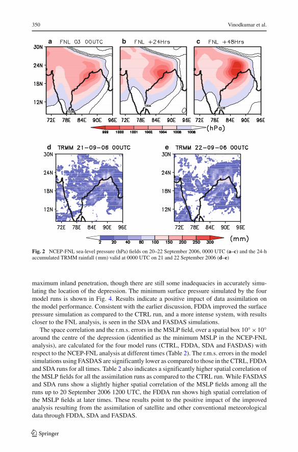
Mean sea-level pressure (MSLP) on 20 September 2006, 0000 UTC and subsequent predicted24- and 48-h fields of the four experiments from the nested domain (12- km grid resolution)are shown in Fig. 3. The model-simulated MSLP fields are compared with those obtainedfrom the NCEP-FNL analyses (Fig. 2a–c). We recognize the drawback in comparing themodel-simulated MSLP with a global model analysis; but this is the best available resourcefor this study domain. From Fig. 3, it can be observed that the movement of the depressionto the land was captured by all of the experiments for the first 24 h, with only the MSLPfrom FDDA showing the minimal change. All experiments except the CTRL show a fur-ther north-westward movement for the next 24 h. The west-north-westward propagation ofmonsoon depressions can be attributed to the prominent characteristic convergence in thenorth-west sector and weak divergence behind the depression (Godbole 1977). Uncharacter-istically, the CTRL experiment shows a south-westward movement on the second day. TheCTRL experiment shows a deeper depression (central MSLP lower by 1 hPa as comparedto the NCEP-FNL analysis) and located off the coast at the initial time, whereas observa-tions indicated that the depression was already located over the land. The depression is seendecaying in the 24-h forecast MSLP from the CTRL experiment while the FNL analyses andweather reports for the time reveal a further intensification. An analysis of the magnitudes ofthe central minimum MSLP predicted by the FDDA experiment and compared to the FNLanalyses at the three times reveals that the predicted values are higher by 2, 3 and 4 hParespectively. The SDA experiment resulted in a deeper system with the central MSLP fieldlower by 1 hPa at the starting time (20 September 2006, 0000 UTC). However, the MSLPfield of the SDA experiment tends to weaken during the first day while intensifying duringthe second day of the forecast. The simulation that shows consistent agreement with theNCEP-FNL analyses is the FASDAS experiment where the depression strengthens on thefirst day and moves inland with a well-marked depression with intensity similar to that inthe NCEP-FNL analyses. Among the four experiments, the FASDAS experiment shows the

123


a b c

d e

Fig. 2 NCEP-FNL sea-level pressure (hPa) fields on 20–22 September 2006, 0000 UTC (a–c) and the 24-haccumulated TRMM rainfall ( mm) valid at 0000 UTC on 21 and 22 September 2006 (d–e)

maximum inland penetration, though there are still some inadequacies in accurately simu-lating the location of the depression. The minimum surface pressure simulated by the fourmodel runs is shown in Fig. 4. Results indicate a positive impact of data assimilation onthe model performance. Consistent with the earlier discussion, FDDA improved the surfacepressure simulation as compared to the CTRL run, and a more intense system, with resultscloser to the FNL analysis, is seen in the SDA and FASDAS simulations.

The space correlation and the r.m.s. errors in the MSLP field, over a spatial box 10◦ ×10◦around the centre of the depression (identified as the minimum MSLP in the NCEP-FNLanalysis), are calculated for the four model runs (CTRL, FDDA, SDA and FASDAS) withrespect to the NCEP-FNL analysis at different times (Table 2). The r.m.s. errors in the modelsimulations using FASDAS are significantly lower as compared to those in the CTRL, FDDAand SDA runs for all times. Table 2 also indicates a significantly higher spatial correlation ofthe MSLP fields for all the assimilation runs as compared to the CTRL run. While FASDASand SDA runs show a slightly higher spatial correlation of the MSLP fields among all theruns up to 20 September 2006 1200 UTC, the FDDA run shows high spatial correlation ofthe MSLP fields at later times. These results point to the positive impact of the improvedanalysis resulting from the assimilation of satellite and other conventional meteorologicaldata through FDDA, SDA and FASDAS.

123


a b c

fed

g h i

j k l

Fig. 3 Sea-level pressure (hPa) simulated by the CTRL (a–c), the FDDA (d–f), the SDA (g–i) and the FASDAS(j–l) runs on 20 September 2006, 0000 UTC and at 24 and 48 h into the forecast

123


0 6 12 18 24 30 36 42 48

996.0

996.5

997.0

997.5

998.0

998.5

999.0

999.5

1000.0

1000.5

1001.0

1001.5

1002.0

1002.5

1003.0

Min

imum

Sea

Lev

el P

resu

re (

hPa)

Integration time (Hrs)

FNL CTRL FDDA SDA FASDAS

Fig. 4 Time series of minimum sea-level pressure (hPa) simulated by the different experiments. 0 correspondsto 20 September 2006, 0000 UTC

Table 2 Space correlation and root-mean-square error of the sea-level pressure field (hPa) for all the fourexperiments (CTRL, FDDA, SDA and FASDAS) with respect to NCEP-FNL analysis for a 10◦ × 10◦ regionaround the depression centre

Date/time (UTC) Spatial correlation RMS error

CTRL FDDA SDA FASDAS CTRL FDDA SDA FASDAS

20/09/2006 0000 0.52 0.77 0.05 0.76 2.79 2.29 2.41 1.77

20/09/2006 0600 0.49 0.63 0.71 0.74 3.33 1.67 1.38 1.19

20/09/2006 1200 0.22 0.55 0.65 0.59 4.98 4.39 3.64 3.35

20/09/2006 1800 0.26 0.93 0.48 0.45 3.51 2.85 2.21 2.07

21/09/2006 0000 0.36 0.95 0.23 0.23 4.53 4.18 3.17 3.03

21/09/2006 0600 0.54 0.64 0.37 0.42 3.46 2.88 2.74 2.50

21/09/2006 1200 0.46 0.65 0.33 0.37 5.41 4.63 3.93 3.52

21/09/2006 1800 0.53 0.65 0.30 0.367 4.23 3.44 3.09 2.56

3.2 Rainfall Fields

The 24-h accumulated total (convective and non-convective) rainfall obtained from all exper-iments is presented in Fig. 5. The upper/lower panels show the 24-h accumulated precipitationvalid until 21/22 September 2006, 0000 UTC for all four experiments. The striking differ-ence in the assimilation runs from the CTRL for the accumulated rainfall on the first dayis the spatial extent of rainfall simulated over land by all of them. Among the assimilationruns themselves, the SDA and FASDAS (the surface data assimilation experiments) simu-lated more rain over land as compared to the FDDA run on the first day. The depressionhad not weakened over land and hence produced abundant rainfall over the north-east, eastand central India as observed in TRMM (Fig. 2d–e). This is well simulated by the SDA andFASDAS experiments as compared to CTRL and FDDA runs. The high intensity rainfall usu-ally observed over the western coast, occurring due to the effect of orography, is reproduced

123


a b c d

e f g h

Fig. 5 24 h accumulated precipitation simulated by CTRL, FDDA, SDA and FASDAS runs valid at 21 and22 September 2006, 0000 UTC

by the SDA and FASDAS runs on the first day. Although the SDA run simulated exten-sive rainfall, mostly over the sea, the observational rainfall pattern from TRMM is in betteragreement with the rainfall simulated by the FASDAS run on the first day. The magnitudeof the maximum precipitation is also higher (>300 mm) for the FASDAS run as comparedto the SDA (<300 mm) run on the first day. The predicted rainfall on the second day alsoshows a similar behaviour with the FASDAS run, simulating more intense rain in terms ofmagnitude as compared to the other three runs, especially on the western coast. The spatialdistribution of rainfall on the second day is seen more over the sea than over the land for allthe simulations, at variance with the observed TRMM rainfall.

3.3 Sub-Surface and Surface Variables

Figure 6 depicts a difference plot of the 0–100 mm layer soil temperature between each ofthe four MM5 model simulations and NCEP-FNL analysis on 20 September 2006 0000,0600, 1200 and 1800 UTC. The model simulations tend to simulate a relatively low soiltemperature compared to the FNL analysis for all the four times plotted. A relative warming(>1 K) is observed over the north-western region in the FDDA run during the daytime (0600and 1200 UTC) but the warming is much less (less than 0.5 K) in the SDA and the FASDASruns. The only positive difference region seen in the CTRL run is noticed at 1200 UTC,and for the rest of the time the CTRL run simulated lower soil temperatures as comparedto the NCEP-FNL analysis. Careful evaluation shows that the two surface data assimilationruns simulated a closer 0–100 mm soil temperature field, especially over central and southernIndia, as compared to the CTRL and FDDA runs at all the first three times (0000, 0600 and1200 UTC 20 September 2006). However at 1800 UTC, all the four model runs simulated alower temperature as compared to the NCEP-FNL all over India. Figure 7 shows the simulateddifference in volumetric soil moisture fraction (×102) for the 0–100 mm layer between the

123


a b c d

hgfe

i j k l

m n o p

Fig. 6 Difference field of the 0–100 mm layer soil temperature (K) between CTRL and NCEP–FNL(a–d), FDDA and NCEP–FNL (e–h), SDA and NCEP–FNL (i–l), and FASDAS and NCEP–FNL (m–p)on 20 September 2006, 0000 UTC, 0600 UTC, 1200 UTC and 1800 UTC

four MM5 numerical experiments and the NCEP-FNL analysis. The differences introducedby different initial conditions are clearly manifest, with an enhancement in the simulatedsoil moisture field in the SDA and the FASDAS runs as compared to the FDDA and theCTRL runs. Despite the improved land-surface representation, inadequacies still exist in the

123


a b c d

hgfe

i j k l

m n o p

Fig. 7 Same as Fig. 6 except for volumetric soil moisture (m3m−3)

model physics, especially with the model’s surface energy balance, as the enhancement insoil moisture is not reflected in the latent heat flux over land (not shown for brevity), exceptfor the FASDAS run on 20 September 2006 0000 UTC.

123


Table 3 Area-averaged surface sensible heat flux over land for a region of 25◦ × 25◦ (sea masked)

Date/time (UTC) Area-averaged sensible heat flux (W m−2)


Sep 20 0000 −26.86 −11.19 −7.42 −8.91 −9.28

Sep 20 0600 28.50 53.46 65.70 56.92 68.54

Sep 20 1200 58.39 −5.65 −3.38 −3.06 −1.79

Sep 20 1800 −24.71 −10.76 −9.61 −10.08 −8.68

Sep 21 0000 −30.12 −11.24 −9.68 −10.16 −9.12

Sep 21 0600 26.43 55.62 53.74 47.63 62.04

Sep 21 1200 64.54 −5.10 −5.36 −4.56 −3.96

Sep 21 1800 −23.39 −11.13 −10.89 −11.16 −10.61

Sep 22 0000 −25.98 −10.15 −10.15 −10.30 −9.84

Table 4 Area-averaged surface latent heat flux over land for a region of 25◦ × 25◦ (sea masked)

Date/time (UTC) Area-averaged latent heat flux (W m−2)


Sep 20 0000 15.39 −1.15 −1.86 0.15 −3.91

Sep 20 0600 176.82 124.07 125.34 150.69 140.09

Sep 20 1200 237.05 7.27 6.84 9.11 7.59

Sep 20 1800 23.83 −0.76 −1.00 0.43 −1.21

Sep 21 0000 21.83 −0.98 −1.05 −0.30 −0.97

Sep 21 0600 180.43 117.38 111.07 112.65 113.41

Sep 21 1200 238.51 6.29 5.70 5.64 6.01

Sep 21 1800 22.91 −0.95 −1.22 −1.02 −0.10

Sep 22 0000 20.17 −1.85 −1.38 −1.11 −1.09

Tables 3 and 4 depict the area-averaged (25◦ × 25◦) values of sensible heat flux (SHF)and latent heat flux (LHF) over the land at different times. The area averaging is limited tothe land region, since the SDA and FASDAS techniques are primarily applied over the land.As seen in the previous case, the MM5 model under-predicts the area-averaged values ofSHF and LHF from NCEP-FNL. The area-averaged SHF (Table 3) simulated by FASDASshows higher values for all times except for the initial time. This shows an enhancement inthe simulated ground temperature by FASDAS, which in turn may affect the atmosphericsurface-layer processes. However, this enhancement in the FASDAS simulated SHF is notseen in the case of LHF (Table 4). It is worth noting that both the surface assimilation runs(SDA and FASDAS) simulated higher values of LHF (by 15–25 W m−2) at 0600 UTC onday one as compared to the CTRL and the FDDA runs. The LHF values at the subsequenttimes of the forecast from each experiment however do not differ much from one another.

3.4 Hovmoller Plots

Figure 8 shows the time evolution of the potential vorticity (PV) field at the model’s lowestlevel (σ = 0.995), over a 180 km × 180 km area about the centre of the depression.

123


a b c d

Fig. 8 Time evolution of the potential vorticity (pvu) field at the model’s lowest level, over a 180 km × 180 kmarea about the centre of the depression

PV analysis is useful for assessing the dynamical impacts of the latent heat release (Brennanet al. 2005). PV maxima are associated with upper troughs, low geopotential heights andcyclonic flow. The consequent increase in the convective motion and enhancement in con-vergence can help explain the intensification of the depression. The CTRL run has simulatedlower PV values as compared to the assimilation (FDDA, SDA and FASDAS) runs. An initialPV maximum of 28 pvu is seen at the centre during the initial stages of the forecast in theCTRL run. A second PV maximum is seen at the end of day one in the CTRL run. Thefollowing two factors generally help to increase the PV below the level of the maximumlatent heat release (LHR): (i) an increased static stability below the level of maximum LHRdue to warming, and (ii) a fall in surface pressure due to warming that leads to convergenceat low levels and to an increase of relative vorticity. An analysis of the MSLP (Figs. 3a–cand 4) of the CTRL shows that the depression was intense at the first two times (20 and21 September 2006, 0000 UTC) and then decayed. This is consistent with the analysis PVstructure. The association of PV with MSLP can also be used to draw broad conclusions ofthe PV pattern obtained from the remaining three experiments of FDDA, SDA and FASDAS.The FDDA run simulated a weak depression as compared to the CTRL, SDA and FASDASruns at 0000 UTC of 20, 21 and 22 September 2006. However the PV field in the FDDA runshows a similar pattern to that from the CTRL run, except over the centre of the depression.The possible reason for the difference of the PV pattern for the FDDA run could be dueto an improvement in the static stability, as compared to the CTRL run, in the assimilationFDDA run. The SDA and the FASDAS runs show enhanced PV values at the initial time,as compared to the SDA and the FASDAS runs showing maxima of 28 and 36 pvu. At the

123


0000 0600 1200 1800 0000 0600 1200 1800 0000

a

b

c

d

e

Fig. 9 Time-height sections of Q1 (K h−1) averaged over a 3◦ × 3◦ area at the centre of the depression,simulated by NCEP-FNL (a), CTRL (b), FDDA (c), SDA (d) and FASDAS (e) runs

end of day one, the maximum PV value simulated by the FASDAS run is 4 pvu higher thanthe SDA run. On day two, another maximum of PV is observed in both the SDA and theFASDAS runs, with the FASDAS run showing a larger spatial extent of the PV field.

3.5 Apparent Heat Source (Q1) and Apparent Moisture Sink (Q2)

The daily variation of Q1(K h−1 for the september 2006 depression −1) averaged over a3◦ × 3◦ box about the depression centre for the NCEP-FNL analysis and for all the fourexperiments is given in Fig. 9. The CTRL experiment (Fig. 9b) shows maximum heating on

123


the first day with a heating rate of about 0.6 K h−1 in the mid-troposphere, around noon localtime (0530 UTC). The maximum heating is usually associated with a large release of latentheat by net condensation as well as the vertical convergence of the vertical eddy transport ofsensible heat (Yanai et al. 1973). The CTRL experiment MSLP fields showed that the systemcrossed land after 24 h (Fig. 3a–c) and weakened on day two of the forecast. This weakeningof the system could be associated with reduced heating due to latent heat of net condensationand lower convergence of vertical transport of sensible heat. The reduction in the heatingrate is characterized by a lower magnitude of Q1 around noon on day two of the forecastfor the CTRL experiment. The FDDA experiment simulated a weak system (Fig. 3d–f) closeto the coast with a nearly stationary system. Q1 in the FDDA experiment (Fig. 9c) suggestsrelatively weak heating on the first day as compared to the CTRL experiment. After 12 hof forecast, the system simulated in the FDDA experiment has crossed land, but has notweakened any further. This manifests as a continuous heating pattern from 1200 UTC onday one until 0900 UTC on day two with the maximum heating (1 K h−1) seen at aroundlocal noon time on the second day. Also, the maximum heating in the FDDA experimentis seen in the upper levels, indicating the presence of cloud clusters over the depressionregion. Compared to the other three experiments, the SDA run (Fig. 9d) shows a small uppertropospheric cooling at 0000 UTC, 20 September 2006. The observed upper troposphericcooling may be due to the overshooting of the rising air in cumulonimbus clouds above thelevel of neutral buoyancy (Ebert and Holland 1992) and the associated radiative cooling ofthe cloud top. While both the CTRL and the FDDA runs show maximum heating aroundlocal noon time, both the SDA and the FASDAS runs (except for the weak heating in theSDA experiment on day one) have their maximum heating at times other than local noon.Another observed feature in the FASDAS runs (Fig. 9e) is an enhanced heating rate towardsthe end of the forecast with values reaching 0.8 K h−1. Such a pattern is observed in theNCEP-FNL analysis (Fig. 9a), with the magnitude of maximum heating in the analysis about0.5 K h−1. The reason for this intense cloud formation and subsequent heating is possiblydue to the enhanced vertical eddy fluxes of sensible heat over land as at this time (end ofday two) the depression had intensified and was well over the land in both the SDA and theFASDAS runs. The amplitude of the surface sensible heat forcing has a strong impact on theconvective boundary-layer formation and hence can affect the area-averaged profiles of Q1.Overall, the SDA run showed a higher magnitude of heating (Q1) as compared to the otherthree experiments with a simulated heat source throughout the period of forecast.

Figure 10 shows the rate of heating due to the apparent moisture sink Q2 for the NCEP-FNL analysis (Fig. 10a), CTRL (Fig. 10b), FEEA (Fig. 10c), SDA (Fig. 10d), and FASDAS(Fig. 10e). Figure 10 shows small negative values of Q2 at the lowest model levels for allthe experiments and for most time. The above mentioned feature is observed in the NCEP-FNL analysis also. It is known that cumulus convection warms the upper troposphere andslightly cools and dries the lower troposphere (Donner et al. 1982). Furthermore, low-levelcooling due to moisture effects may be due to the dominance of re-evaporation of the dropletsbecause of strong winds associated with the intense depressions simulated by each of thefour experiments (Ratnam and Cox 2006). Overall, the Q2 pattern is quite similar to the Q1

pattern except for the absence of heating at the end of day two in the SDA experiment and anincrease in the maximum heating rate of about 0.2–0.4 K h−1 as compared to Q1. Q2 beingthe measure of vertical eddy transport of moisture, the positive value of Q2 is due to thepresence of deep convection that has developed in a convectively active environment. Themaximum heating due to moisture seen at 0000 UTC of 22 September 2006 in the FASDASrun can be attributed to the deep convection formed due to the surface latent heat forcingsupplied by the higher inland soil moisture, together with the moist environment in the

123


0000 0600 1200 1800 0000 0600 1200 1800 0000

a

b

c

d

e

Fig. 10 Same as Fig. 9 except for Q2 (K h−1)

middle troposphere. This early morning deep convection and associated rainfall over trop-ical land is also seen in the results of Gray and Jacobson (1977) and Zuidema (2003). Theabove mentioned heating pattern obtained in FASDAS at 22 July 2006 0000 UTC is observedin the FNL analysis also.

In Fig. 11a, a time-averaged vertical profile of the area-averaged Q1 is shown from all thefour numerical experiments for the September 2006 depression. The vertical profile of Q1

shows a large heating in the middle and upper levels for all the experiments, with the NCEP-FNL, CTRL, FDDA, SDA and FASDAS runs showing maximum values of about 4.2, 2.5, 3.7,5.0 and 4 K day−1, respectively. The enhancement in the time-averaged and area-averagedrate of heating due to the apparent heat source in the SDA and the FASDAS runs may be due

123


Fig. 11 48 h time-averagedvertical profiles of area-averagedQ1 (a) and Q2 (b) from theNCEP-FNL and the four modelexperiments. For all thesimulations, area averaging is for10◦N–25◦N, 72◦E–95◦E

Q1

Q2

a

b

123


to the better convective initiation, which is a result of the better simulation of surface andboundary-layer processes via surface data assimilation. The diagnosed apparent heat sourceQ1 from the four numerical experiments shows a cooling at the higher levels. Some of thephysical processes, such as cloud-top radiational cooling, anvil evaporation, and turbulentmixing of stratospheric and tropospheric air resulting from overshooting cumulonimbus tops,may possibly produce cooling at this level (Kuo and Anthes 1984).

The time- and area-averaged vertical profile of Q2 (Fig. 11b) shows a low-level coolingand an upper level heating for all the four experiments. However, the NCEP reanalysis showsa low-level heating, a feature different from all the model results. The level of maximumheating in the NCEP-FNL is low (sigma level 0.825) compared to that seen in the modelruns. It can be seen from Fig. 11b that the magnitude of cooling is highest for the SDA runfollowed by the FASDAS run. Furthermore, the magnitude of the upper-level heating is leastfor the CTRL run while it is higher for all the three assimilation runs (Fig. 11b) with theSDA run having the maximum value of heating. The maximum of the convective heat source(Q1) occurs at a height different from the height of the peak of the apparent moisture sink(Q2), mainly because condensation occurs in narrow convective updrafts. Earlier studieshave shown that the height of the maximum of the convective heat source (Q1) is unusuallyhigher than the height of the peak of the apparent moisture sink (Q2). This feature is seen forall the experiments except for the SDA run. Over all, the apparent heat source and apparentmoisture sink have the highest heating rates for the SDA run followed by the FASDAS run.

4 Quantitative Validation

4.1 Errors in Near-Surface Variables

Table 5 depicts the mean error, absolute error and the standard deviation for temperature(T), dewpoint temperature (Td), wind speed (V) and wind direction (Dir) with respect tothe surface observations averaged for the period 20–22 September 2006. While the FDDArun simulated the lowest error in the simulation of temperature and dewpoint temperature,the FASDAS run had the minimum error for the wind speed, and wind direction. However, theerror values, especially those of temperature and wind speed, are somewhat higher than theaccuracy requirement of Cox et al. (1998). These large errors can be attributed to the use ofGFS forecast fields to initialize the model, while initializing the MM5 with global analyses,such as the NCEP-FNL analysis, would have reduced the errors considerably. Moreover, theassimilated ATOVS data have some limitations, since the retrieved temperature and dew-point temperature have only an accuracy of 2 and 3–6 K respectively (Li et al. 2000). Also,

Table 5 Mean error, absolute error, and the standard deviation of the difference between the IMD surfaceobservations and the MM5 model simulations for 20–22 September 2006

Variable Mean error Absolute error Standard deviation

CTRL FDDA SDA FASDAS CTRL FDDA SDA FASDAS CTRL FDDA SDA FASDAS

T (K) 1.66 1.41 2.27 2.09 3.48 3.37 3.9 3.81 4.49 4.43 4.96 4.82

Td (K) 1.18 0.71 0.96 0.97 2.45 2.06 2.38 2.23 3.36 3.11 3.29 3.19

V (m s−1) −3.04 −2.82 −2.89 −2.55 3.46 3.22 3.39 3.06 3.38 3.15 3.35 3.16

Dir. (deg) 19.71 16.3 14.42 10.58 57.3 52.97 54.81 53.44 73.07 70.79 71.85 69.35

123


the dense wind information from QuikSCAT is limited over the sea, and overland the onlyavailable source of wind data is conventional wind observations, which needless to say aresparse.

4.2 Statistical Significance of r.m.s. Errors of Temperature, Dewpoint Temperatureand Wind Speed

To investigate the significance of the statistics of the r.m.s. errors of temperature, dew-point temperature and wind speed, it was decided to apply the student’s t-test to r.m.s.errors of each of the assimilated runs with respect to the CTRL run to bring out thestatistical significance of assimilation The r.m.s. errors were calculated at nine levels(1000, 925, 850, 700, 600, 500, 400, 300, and 200 hPa) for the above mentioned vari-ables with respect to the radiosonde data. However for brevity, the r.m.s. errors are notshown here. For each variable and at each pressure level, the significance statistics werecalculated over 3 days at a 12 hourly interval (frequency of the radiosonde observations).The r.m.s. error of temperature for the three assimilation runs (FDDA, SDA and FAS-DAS) shows 99% significance level at all the vertical levels with respect to the CTRLrun. The dewpoint temperature of the FDDA run shows a significance of 99% for allthe levels except the 600- and 300-hPa levels with respect to the CTRL run. The windspeed also shows a significance of 99% at all the pressure levels for the FDDA run ascompared to the CTRL run. The SDA run showed that the statistical significance of ther.m.s. error of dewpoint temperature was 99% except at 1000, 600, and 300 hPa withrespect to the CTRL run. For the wind speed, the only statistically insignificant levelswith value less than 90% is the 1000-hPa level. A statistical significance of 99% wasseen for dewpoint temperature at the pressure levels of 925, 600, 400 and 200 hPa inthe case of the FASDAS run as compared to the CTRL run. For wind speed, the FAS-DAS runs exhibited a statistical significance of 99% at all levels, as in the case of theFDDA run.

5 Summary and Conclusions

Two approaches of surface data assimilation were implemented along with the conventionalFDDA to study the impact of different assimilation approaches on the simulation of a mon-soon depression over India. A case study of the 21 September 2006 Bay of Bengal monsoondepression was used with particular focus on the role of land atmosphere interactions onthe evolution of the monsoon event. The study provides one of first comparisons of twosurface data assimilation techniques for a comparison of a large-scale system such as themonsoon depression over India. The model results were compared with one another andwith the NCEP-FNL analysis and TRMM estimates. In the model runs, data assimilationwas restricted to the first 24 h of the integration, and subsequently the model was run in afree forecast mode. Results suggest that the FASDAS run performed better than the otherruns, highlighting the benefit of assimilating satellite and conventional upper air and surfaceobservations through FASDAS and FDDA over the Indian monsoon region.

Study results can be summarized as follows.

(i) Improved realistic simulations of surface/near-surface fields of temperature, moisture,sensible and latent heat fluxes were observed in all the three assimilation (FDDA, SDAand FASDAS) experiments as compared to the CTRL experiment.

123


(ii) The FASDAS run simulated MSLP fields showed an improvement in terms of intensityand movement of the monsoon depression. The FASDAS run had the lowest r.m.s.error of MSLP for the entire duration of the forecast.

(iii) Although the changes in the surface fluxes, surface air temperature and humidity weremodest, these changes introduced horizontal gradients that influenced the magnitudeand the distribution of precipitation as well as in the evolution of the boundary layerand convection. A qualitative evaluation of the precipitation forecasts from all the fourexperiments revealed that the FASDAS run simulated precipitation in good agreementwith the TRMM estimates.

(iv) The SDA experiment simulated stronger heating/cooling through apparent heat andmoisture sources, which led to a greater interaction between convection and the large-scale tropical motions. Even though the SDA simulated higher heating rates than theFASDAS run, it simulated the peak of the convective heat source at a height lowerthan the peak of the apparent moisture sink, a feature not very realistic and not seenin the other three experiments.

A potential limitation of the study is the errors in the derived ATOVS satellite observationsthat were assimilated. Since there were no other reliable sources for surface and soundingdata over the sea other than satellites, we had to rely on the available data. Future observa-tional capabilities over the Indian monsoon region should provide enhanced surface fieldsthat can positively impact upon the simulation of monsoon depressions, as revealed frompresent results.

An important conclusion from this study is that even though monsoon depressions are largesynoptic systems, mesoscale features, including rainfall, is affected by surface processes.Enhanced representation of land-surface processes provide a significant improvement in themodel performance even under active monsoon conditions where the synoptic forcings areexpected to be dominant.

Acknowledgments The authors thank NCAR for access to the MM5 model, National Climatic Data Centrefor GFS forecasts, NCEP for the FNL analysis and NASA for the NOAA-TOVS, TRMM, and QuikSCATdatasets. The authors also thank the IMD for providing RS, RW, PB and surface data. Thanks are also dueto the UK Met Office for the ATOVS/AVHRR processing package, and to the University of Wisconsin forIAPP. A special thanks to Dr. Hal Woolf for his invaluable support on IAPP. The first author acknowledgesthe Council of Scientific and Industrial Research, India for providing a research fellowship to carry out thepresent work. DN was supported in part from NSF CAREER ATM-0897227 (Drs. Liming Zhou and Jay Fein),NASA Terrestrial Hydrology (Dr. Jared Entin), and NOAA JCSDA.

References

Alapaty K, Raman S, Niyogi D (1997) Uncertainty in the specification of surface characteristics: a study ofprediction errors in the boundary layer. Boundary-Layer Meteorol 82:475–502

Alapaty K, Seaman NL, Niyogi DS, Hanna AF (2001) Assimilating surface data to improve the accuracy ofatmospheric boundary layer simulations. J Appl Meteorol 40:2068–2082

Alapaty K, Niyogi D, Chen F, Pyle P, Chandrasekar A, Seaman N (2008) Development of the flux-adjustingsurface data assimilation system for mesoscale models. J Appl Meteorol Climatol 47:2331–2350

Bouttier F, Mahfouf JF, Noilhan J (1993) Sequential assimilation of soil moisture from atmospheric low-levelparameters part I: sensitivity and calibration studies. J Appl Meteorol 32:1335–1351

Brennan MJ, Lackmann GM, Mahoney KM (2005) Potential vorticity as a tool for assessing dynamicalimpacts of latent heat release in model forecasts. In: 21st Conference on weather analysis and forecast-ing/17th conference on numerical weather prediction. American Meteorological Society, WashingtonDC, CD-ROM, 14A.3.

123


Carlson TN, Gillies RR, Schmugge TJ (1996) An interpretation of methodologies for indirect measurementof soil water content. Agric For Meteorol 77:191–205

Chen F, Dudhia J (2001) Coupling an advanced land-surface/hydrology model with the Penn State/NCARMM5 modelling system Part I: model implementation and sensitivity. Mon Weather Rev 129:569–585

Chen F, Mitchell K, Schaake J, Xue Y, Pan HL, Koren V, Duan QY, Ek K, Betts A (1996) Modeling of land-surface evaporation by four schemes and comparison with FIFE observations. J Geophys Res 101:7251–7268

Cox R, Bauer BL, Smith T (1998) A mesoscale model inter-comparison. Bull Am Meteorol Soc 79:265–283Donner LJ, Kuo HL, Pitcher EJ (1982) The significance of thermodynamic forcing by cumulus convection in

a general circulation model. J Atmos Res 39:2159–2181Dudhia J (1989) Numerical study of convection observed during winter monsoon experiment using a meso-

scale two-dimensional model. J Atmos Sci 46:3077–3107Ebert EE, Holland GJ (1992) Observations of record cold cloud-top temperatures in Tropical Cyclone Hilda

(1990). Mon Weather Rev 120:2240–2251English SJ, Renshaw RJ, Dibben PC, Smith AJ, Rayer PJ, Poulsen C, Saunders FW, Eyre JR (2000) A com-

parison of the impact of TOVS and ATOVS satellite sounding data on the accuracy of numerical weatherforecasts. Q J Roy Meteorol Soc 126:2911–2931

Garratt JR, Hess GD, Physick WL, Bougeault P (1996) The atmospheric boundary layer—advances in knowl-edge and application. Boundary-Layer Meteorol 78:9–31

Godbole RV (1977) The composite structure of the monsoon depression. Tellus 29:25–40Gray WM, Jacobson RW (1977) Diurnal variation of deep cumulus convection. Mon Weather Rev 105:1171–

1188Grell GA, Dudhia J, Stauffer DR (1994) A description of the fifth-generation Penn State/NCAR mesoscale

model (MM5), NCAR Technical Note TN-398+STR, National Center for Atmospheric Research,Boulder, CO

Hong SY, Pan HL (1996) Non-local boundary layer vertical diffusion in a medium-range forecast model. MonWeather Rev 124:2322–2339

Krishnamurti TN, Xue H, Bedi HS, Ingles K, Oosterhof D (1991) Physical initialization for numerical weatherprediction over the tropics. Tellus A 43:53–81

Kuo YH, Anthes RA (1984) Mesoscale budgets of heat and moisture in a convective system over the centralUnited States. Mon Weather Rev 112:1482–1497

Lakshmi V (2000) A simple surface temperature assimilation scheme for use in land surface models. WaterResour Res 36:3687–3700

Li J, Wolf WW, Menzel WP, Zhang W, Huang HL, Achtor TH (2000) Global soundings of the atmospherefrom ATOVS Measurements: the algorithm and validation. J Appl Meteorol 39:1248–1268

Mahfouf JF (1991) Analysis of soil moisture from near surface parameters: a feasibility study. J Appl Meteorol30:1534–1547

McNider RT, Song AJ, Casey DM, Wetzel PJ, Crosson WL, Rabin RM (1994) Towards a dynamic-thermo-dynamic assimilation of satellite surface temperature in numerical atmospheric models. Mon WeatherRev 122:2784–2803

McNider RT, Lapenta WM, Biazar A, Jedlovec G, Suggs R, Pleim J (2005) Retrieval of grid scale heat capacityusing geostationary satellite products: part I: case-study application. J Appl Meteorol 88:1346–1360

Niyogi D, Raman S, Alapaty K (1999) Uncertainty in specification of surface characteristics, Part 2: hierarchyof interaction explicit statistical analysis. Boundary-Layer Meteorol 91:341–366

Niyogi D, Pielke RA Sr, Alapaty K, Eastman J, Holt T, Mohanty UC, Raman S, Roy TK, Xue Y-K (2002)Challenges of representing land surface processes in weather and climate models over tropics: examplesover the Indian subcontinent. In: Weather and climate modeling. New Age International, New Delhi,300 pp

Niyogi D, Alapaty K, Raman S, Chen F (2009) Development and evaluation of a coupled photosynthesis-based gas exchange evapotranspiration model (GEM) for mesoscale weather forecasting applications.J Appl Meteorol Climatol 48:349–368

Pleim JE, Xiu A (2003) Development of a land surface model. Part II: data assimilation. J Appl Meteorol42:1811–1822

Ramamurthy MK, Carr FH (1987) Four-dimensional data assimilation in the monsoon region. Part I: experi-ments with wind data. Mon Weather Rev 115:1678–1706

Ratnam VJ, Cox EA (2006) Simulation of monsoon depressions using MM5: sensitivity to cumulus parame-terization schemes. Meteorol Atmos Phys 93:53–78

Ruggerio FH, Sashegyi KD, Madala RV, Raman S (1996) The use of surface observations in four-dimensionaldata assimilation in a mesoscale model. Mon Weather Rev 124:1018–1033

123


Singh R, Pal PK, Kishtawal CM, Joshi PC (2008) The impact of variational assimilation of SSM/I and Quik-SCAT satellite observations on the numerical simulation of Indian ocean tropical cyclones. WeatherForecast 23:460–476

Stauffer DR, Seaman NL, Binkowski FS (1991) Use of four-dimensional data assimilation in a limited areamesoscale model. Part II: effects of data assimilation within the planetary boundary layer. Mon WeatherRev 119:734–754

Vinodkumar, Chandrasekar A, Alapaty K, Niyogi D (2008) The impacts of indirect soil moisture assimilationand direct surface temperature and humidity assimilation on a mesoscale model simulation of an Indianmonsoon depression. J Appl Meteorol Climatol 47:1393–1412

Yanai M, Esbensen S, Chu JH (1973) Determination of bulk properties of tropical cloud clusters from large-scale heat and moisture budgets. J Atmos Sci 30:611–627

Zuidema P (2003) Convective clouds over the Bay of Bengal. Mon Weather Rev 131:780–798

123

assessment of data assimilation approaches for the ... vinodkumar et al. vorticity. heat and...

Documents