assessment of historical and future water availability in

Assessment of Historical and Future WaterAvailability in Himalayan Tamor River Basin NepalUtilizing CMIP5 CNRM Climate Model ExperimentsBishal Pokhral

IIT Roorkee: Indian Institute of Technology RoorkeeVishal Singh ( [email protected] )

National Institute of Hydrology https://orcid.org/0000-0001-6023-7075S. K. Mishra

IIT Roorkee: Indian Institute of Technology RoorkeeSanjay K Jain

National Institute of HydrologyPushpendra K Singh

National Institute of HydrologyJoshal K Bansal

National Institute of Hydrology

Research Article

Keywords: Tamor Basin, SWAT Modeling, Water Availability, Climate change, Dependable Flow, CMIP5CNRM

Posted Date: November 2nd, 2021

DOI: https://doi.org/10.21203/rs.3.rs-855294/v1

License: This work is licensed under a Creative Commons Attribution 4.0 International License. Read Full License

https://doi.org/10.21203/rs.3.rs-855294/v1

mailto:[email protected]

https://orcid.org/0000-0001-6023-7075

https://doi.org/10.21203/rs.3.rs-855294/v1

https://creativecommons.org/licenses/by/4.0/

1

Assessment of Historical and Future Water Availability in Himalayan Tamor River Basin 1

Nepal Utilizing CMIP5 CNRM Climate Model Experiments 2

1Bishal Pokhral, 2Vishal Singh*, 1S. K. Mishra, 2Sanjay Kumar Jain, 2Pushpendra Kumar 3

Singh, 2Joshal Kumar Bansal 4

1Water Resources Development and Management, Indian Institute of Technology, Roorkee-5

247667, Uttarakhand, India 6

2Water Resources System Division, National Institute of Hydrology, Roorkee-247667, 7

Uttarakhand, India 8

9

10

11

*Corresponding Author - Dr. Vishal Singh 12

Email – [email protected] 13

14

15

16

17

18

19

20

21

2

Assessment of Historical and Future Water Availability in Himalayan Tamor River Basin 22

Nepal Utilizing CMIP5 CNRM Climate Model Experiments 23

1Bishal Pokhral, 2Vishal Singh*, 1S. K. Mishra, 2Sanjay Kumar Jain, 2Pushpendra Kumar 24

Singh, 2Joshal Kumar Bansal 25

1Water Resources Development and Management, Indian Institute of Technology, Roorkee-26

247667, Uttarakhand, India 27

2Water Resources System Division, National Institute of Hydrology, Roorkee-247667, 28

Uttarakhand, India 29

Abstract: In this study, the assessment of water availability under climate changing 30

environment has been done in the Himalayan Tamor River Basin, Nepal using physically 31

based, spatially distributed, a continuous model 'Soil and Water Assessment Tool' (SWAT). 32

The hydrological simulation and projection have been performed in the historical (1996-2007) 33

and future times (e.g. 30s, 40s, 50s, 60s, 70s, 80s, 90s). The climate change impact assessment 34

on the hydrology of Tamor river basin has been performed utilizing the CMIP5 CNRM climate 35

model datasets (with RCP4.5 and RCP8.5). The model calibration and parameterization 36

uncertainty evaluation in the simulated and projected flows were done in SWATCUP using 37

SUFI2 algorithm. The results obtained from the model calibration (1996-2004) and validation 38

(2005-2007) showed a reliable estimate of daily streamflow for calibration period (R2 = 0.85, 39

NSE =0.85 and PBIAS=-2.5) and validation period (R2 =0.87, NSE =0.85 and PBIAS=-5.4). 40

The average annual water yield at the main outlet of the basin is computed as 1511.13 mm, and 41

the total annual quantity is recorded as 6.25 BCM. The average annual precipitation over the 42

seleced river basin is projected to be increased in all scenarios. The stations at higher altitude 43

show more temperature rise than those at a lower elevation and thus there would be minimal 44

snowfall has been projected in the basin by 2100 AD under both scenarios (RCP4.5 and 45

3

RCP8.5). It is expected that the flow pattern in the future would be similar to the baseline 46

pattern under all scenarios. The baseflow will be dramatically increased in all scenarios, but 47

the lowest flow month would be shifted from March to February. Since the base flow during 48

lean months would be increased in future as projected by all scenarios, there would not be 49

adverse impacts on higher percentile flows. This study would be useful for the assessment of 50

the possibility of storage type or run-off-river type hydro-project in the basin in terms of water 51

availability. 52

Keywords: Tamor Basin; SWAT Modeling; Water Availability; Climate change; Dependable 53

Flow, CMIP5 CNRM 54

1. Introduction 55

The water resource is one of an essential input to the growth and well-being of the nation. 56

Nepal is a mountainous country with more than 6000 rivers, with a total average yearly flow 57

of about 225 billion cubic meters (WECS, 2011). As other mountain originated river of Nepal, 58

Tamor river is being planned for its extensive use especially in hydropower generation and 59

highly linked for inter-basin transfer being excess in the basin than demand. Nepal has realised 60

as a national topmost and highly prioritised issue of water resources for the country prosperity 61

and development (Chhetri et al., 2020; Sharma and Shakya, 2006). But the hydrology of the 62

rivers in Himalayan basin is predicted to be more vulnerable because of the seasonal, latitudinal 63

and altitudinal shifting of the freezing line due to the effects of the climate change (Singh et 64

al., 2021a; Singh and Goyal, 2017; Jones, 1999). 65

The rate of snowfall can be determined for precipitation with the record of daily air 66

temperature. (Pradhanang et al., 2011). The rising of atmospheric temperature is the leading 67

cause of the declining the quantity of snowfall in the Himalayan regions which further result 68

in the rapid melting of snow-glaciers and reduces the snow cover durations (Singh et al., 2021a, 69

4

2021b; Singh and Bengtson, 2004). The reduction of the snow-to-rain ratio causes wetter 70

monsoon and drier lean flow seasons which has a very adverse effect on the runoff river type 71

hydropower potential of the mountain rivers (Singh et al., 2021b; Agrawala et al., 2003). 72

Nowadays, several hydrological models are available for an efficient assessment of water 73

resources and to find out the impact of climate and soil properties on hydrology and water 74

resources. (Shrestha et al., 2015; Moradkhani and Sorooshian, 2009) defined a model as a 75

simplified representation of the real-world system. 76

The best model is that which gives results proximity to reality with the use of least possible 77

parameters and model complexity (Devia et al., 2015). Among different process-based semi-78

distributed models, SWAT which can perform on HRU level has been used extensively and 79

globally for the simulation and projection of various hydrological components (Singh et al., 80

2019; Singh and Goyal, 2017; Jain et al., 2017). Many studies provided an overview of the 81

model performance statistics for hydrological processes in numerous SWAT applications 82

(Himanshu et al., 2017; Pandey et al., 2015; Gassman et al., 2014). Several studies 83

demonstrated the model performance in the projection of hydrological components in 84

Himalayan basins utilizing multi-model climate datasets to assess the impact of climate change 85

(Singh et al., 2019; Singh and Goyal, 2017). Mishra et al. (2018) explored the effects of climate 86

change on streamflow in the Bheri river basin Nepal with three GCMs under RCP4.5 and 87

RCP8.5 and predicted that due to increase in maximum and minimum temperature in future, 88

the streamflow increases. 89

Kundu et al. (2017) studied individual and combined effects of land-use and climate change on 90

the Narmada River basin, India and concluded that the climate change has more influence on 91

water yield and land-use change was affecting more on evapotranspiration and overland flow. 92

A very few studies analyzed that the supply and demand of water in the Himalayan basin is 93

5

affected by the effects of climate changes on glacier dynamics (Singh et al., 2021b; Singh et 94

al., 2019a; NRCNA 2012). Singh and Goyal (2016) analysed temperature and precipitation in 95

Tista river catchment in India with CMIP5 climate model datasets and observed that there were 96

substantial variations in streamflow and precipitation in terms of their rates, intensities and 97

frequencies in observed as well as future periods. 98

Since very limited studies have been recorded to assess the future water availability under the 99

influence of climate change in snow and glacial dominated mountainous terrain of Nepal, the 100

reviews of various kinds of literature mentioned above encouraged for the application of the 101

SWAT model for hydrologic simulation and projection of various hydrological components 102

over the Himalayan Tamor River basin, Nepal. The SWAT model has been performed on the 103

daily scale, but the outcomes have been studied at daily, monthly and annual scales. The 104

undertainty in the modeling outcomes has been assessed during model calibration with 105

reference to observed streamflow data utilizing SUFI-2 optimization method which is inbuilt 106

in SWATCUP. The uncertainty estimation using SUFI-2 was done by many researchers, which 107

is found effective in the improvements of projected modeling scenarios using SWAT (Kumar 108

et al., 2017; Singh and Goyal, 2017). Since a large size Dam of about 208 m is proposed at the 109

outlet location of the selected river basin for the construction of Tamor Storage Hydroelectric 110

Project. However, this is not a hydrological station and does not have a measured dataset of 111

any periods. Thus, the simulated discharge at the outlet obtained from this study would be very 112

useful for the generation of hydropower potential in the selected river basin. Similarly, the 113

predicted future streamflow will further help to understand the future pattern and future water 114

potential of the river. The water availability over the basin has been assessed by computing the 115

probabilistic dependable flows in historical and future times by constructing Flow Duration 116

Curves (FDCs). The climate change impacts on the water availability have been assessed 117

utilizing the CMIP5 CNRM-CM5 climate model experiments (with RCP4.5 and RCP 8.5). 118

6

2. Study Area 119

Koshi river is the largest river of Nepal, and among its seven major sub-basins, the Tamor sub-120

basin is the easternmost sub-basin that originates from the Himalayas of Kanchanjunga and 121

joins with Arun and Sunkoshi to form giant Saptakoshi which is the major tributary of Ganga 122

River in India. The basin area considered in this study is 4860.5 Km2 from Taplejung, 123

Terhathum and Panchthar districts of Province no. 1, Nepal. The basin has a very diverse 124

climate since the elevation ranges from 350 m to 7526 m above mean sea level within 150 km 125

length. The south-east monsoon is the most dominant climatic influence and is responsible for 126

almost monsoon in the basin. The difference between the warm and humid summer and the 127

extremely cold winter becomes remarkable with the increase in altitude from South to North. 128

The mean annual basin precipitation is around 2305 mm (a result of this study). Although, most 129

of the precipitation for this region is concentrated during the monsoon months, the snow-130

covered and glaciated upper reaches of the basin contribute meltwater to the streamflow 131

throughout the year. Furthermore, other spring sources in the hilly and mountain terrains 132

provide considerable perennial water discharge in the basin. Besides, freshwater streams, 261 133

glaciers and 356 glacial lakes are recorded within the basin area (ICIMOD,2001). In this study, 134

Majhitar station (catchment area-4132 km2) is calibrated whose average annual observed flow 135

for (1996–2004) is 265.5 m3/s (data from DHM, Nepal). The main outlet of the basin in this 136

study corresponds to the Dam site of proposed Tamor river hydropower project of 762 MW 137

(NEA Nepal, 2018). But this is not a hydrological station, and hence the discharge data at 138

Majhitar will be calibrated in this study for the estimation of simulated flow at this outlet. The 139

future predicted discharge under various scenarios in this study would provide crucial 140

information on future water availability at the dam location and help in making sustainable 141

planning for reservoir operation. 142

**Insert Figure 1 here** 143

7

3. Data Inputs Utilized 144

It is always essential to use all relevant and high-quality data to obtain a good result. The 145

essential input datasets are digital elevation model (DEM), soil map, land use and land cover 146

(LULC) map, slope map, weather generator data and observed discharge were used for the 147

SWAT modeling simulation and calibration (Figure 2). 148

In this study, the SRTM DEM of 30m × 30m resolution has been used to delineate the streams, 149

sub-basins, slope, basin boundary and other watershed parameters 150

(https://earthexplorer.usgs.gov/). LULC data was obtained from the International Centre for 151

Integrated Mountain Development (ICIMOD) and then it was reclassified using crops and land 152

use types that were defined within the model databases and used for the creation of multiple 153

Hydrologic Response Units (HRUs). The watershed area of the Tamor river is mostly occupied 154

by dense forest to deciduous forest, agricultural and snow-covered area (Figure 2). The textural 155

and physicochemical properties of soil such as soil texture, hydraulic conductivity, water 156

content, bulk density, organic matter content etc. for different layers of each soil type are 157

required for SWAT modeling. 158


The soil map and soil parameters were obtained from Food and Agricultural Organization 160

(FAO) with a scale of 1:50,00,000 for the study area 161

(http://www.fao.org/geonetwork/srv/en/metadata.show?id=14116). Dystic Cambisols (Bd34-162

2bc) is found the dominant soil class in the basin area followed by Lithosols (I-Bh-U-c-3717) 163

(Figure 2). The slope map of the study area was prepared from the SRTM DEM and then it 164

was re-classified into five different classes (Figure 2a). The Tamor river basin is mostly 165

characterised by mild to a high steep slope. 166

8

The daily meteorological data from 1993-2007 were used by the SWAT model for the analysis 167

of water balance at HRU scale and its aggregation was done at sub-basin and watershed scale. 168

The daily precipitation data of twelve stations, five temperature stations and measured 169

discharge data of Majhitar outlet were obtained from the Department of Hydrology and 170

Meteorology (DHM), Nepal have been used for the study analysis. The location of the 171

meteorological and hydrological stations within or in the proximity of the basin has shown in 172

the Figure 2b. The auto simulation option available in ArcSWAT was chosen for remaining 173

data input, such as wind speed, relative humidity, and solar radiation, which utilizes the datasets 174

from the weather generator of SWAT. Before using the rainfall and temperature data in the 175

application, it was checked for continuity, and missing rainfall and temperature records were 176

filled by the data data-gaps filling method such as multi-linear regression (MLR) and Inverse 177

Distance Weightage (IDW) methods (Singh and Xiaosheng, 2019; Chen et al., 2017). 178

4. Methodology 179

4.1 SWAT Modeling For Snow/Glacier Induced Basin 180

SWAT requires number of data inputs viz. DEM, LULC map, soil map, slope (Figure 4a) and 181

hydro-meteorological datasets to setup the model. The present study basin corresponded to 182

snow and glaciers and therefore, several additional parameters relevant to snow/glacier 183

hydrology were also taken into consideration with parameters related to rainfall-runoff 184

modeling. In this study, the basin, sub-basins, and drainage networks were delineated with the 185

help of ArcSWAT interface using DEM data. The whole study basin was divided into 15 sub-186

watersheds (see Figure 2b). While deciding the sub-basin outlets, important un-gauged 187

locations needing water resource assessment and available river gauging stations were 188

considered. A total of eight LULC classes and four types of soil were defined (Figures 4c and 189

4d). The land slope of the study was classified into five multiple classes and overlaid with the 190

9

LULC and soil map and the threshold value of 8% each for land use, soil and slope was defined 191

which divided the total watershed into 298 number of hydrologic responsive units (HRUs). 192

Similar subwatershed is characterised by dominant land use, soil type and management 193

practices (Kalcic et al., 2015). Snow cover and snowmelt are simulated separately for each 194

elevation band (Fontaine et al., 2002). The SWAT allows the users to split sub-basins into a 195

maximum of ten elevation bands, but only eight elevation bands were set up for the snow, and 196

glacial dominated sub-basins in higher altitudes with an equal vertical distance from the mean 197

elevation of the centroid of the sub-basins. The model was run considering the following 198

methods of calculation for various hydrological processes; Penman-Monteith method for 199

potential evaporation process, SCS Curve number for surface runoff, initial curve number 200

estimation using soil moisture method, Muskingum method for channel routing. 201

4.2 SWAT CUP – Calibration, Model Parametrization and Sensitivity analysis 202

The SWAT-CUP, a public domain software which is easily linked to the SWAT interface of 203

GIS, was used for the calibration/ uncertainty or sensitivity analysis. The details about SWAT-204

CUP can be read on (Abbaspour, 2015). The SUFI2 model was chosen for its advantages over 205

other algorithms of covering all types of uncertainties like, (a) uncertainty of input variables 206

like precipitation; (b) uncertainty in the concept of the model; (c) uncertainty in the used 207

parameters and (d) uncertainty of observed data. In SUFI-2, the degree of uncertainties is 208

enumerated by a measure specified as the P-factor (i.e. the percent of measured data bracketed 209

by the 95% prediction uncertainty (95PPU)) and quantify the strength of the uncertainty 210

analysis by R-factor (i.e. the average thickness of the 95PPU band divided by the standard 211

deviation of the measured data). SUFI-2 tends to cover most of the measured data with the 212

smallest possible uncertainty band. (Abbaspour, 2015). In general, hydrological models such 213

as SWAT incorporate many parameters, but only a few of these parameters have sensitive 214

impacts. 215

10

SWAT-CUP has two options for sensitivity analysis, and they are all-at-a time (AAT), i.e. 216

global and one at a time (OAT) sensitivity analysis. In this study, a global sensitivity analysis 217

was chosen since the AAT produces more reliable results than OAT (Abbaspour, 2015). Global 218

sensitivity analysis is determined based on t-stat and p-value (Abbaspour, 2015). At 95% 219

confidense interval, as per the t-stat test, if the value of parameter exceeds >2.0 or less than -220

2.0, the parameter can be defined as the significant sensitive. While, in case of p-value test, 221

parameters having values <0.05 can be defined as significant sensitive (Abbaspour, 2015). In 222

SUFI-2, the calibration was done from 1996 to 2005, and the result from calibration was further 223

validated for 2005 to 2007 at the Majhitar outlet. The optimized parameters after the calibration 224

in SWAT-CUP will be aggregated over the downstream subbasins (14 and 15) to get the 225

reliable predictions at the final outlet location of the selected river basin. The evaluation of 226

model performance or the measure of the degree of fit was done taking three most common 227

objective functions in SWAT CUP, Nash-Sutcliffe efficiency (NSE) (Lin et al., 2017), 228

Coefficient of Determination (R2) (Aawar et al., 2020) and the percentage bias (PBIAS) 229

(Zhang et al., 2019). 230

𝑅2 = [ ∑ (𝑄𝑚,𝑖 − 𝑄𝑚) (𝑄𝑠,𝑖 − 𝑄𝑠)𝑖=𝑛𝑖=1[∑ (𝑄𝑚,𝑖 − 𝑄𝑚)2 ∑ (𝑄𝑠,𝑖 − 𝑄𝑠)2𝑛𝑖=1𝑖=𝑛𝑖=1 ]]2 Eq. 1

𝑁𝑆𝐸 = 1 − [ ∑ (𝑄𝑚,𝑖 − 𝑄𝑠,𝑖)2𝑖=𝑛𝑖=1∑ (𝑄𝑚,𝑖 − 𝑄𝑚,𝑖 )2𝑖=𝑛𝑖=1 ] Eq. 2

𝑃𝐵𝐼𝐴𝑆 = [∑ (𝑄𝑚,𝑖 − 𝑄𝑠,𝑖) ∗ 100𝑖=𝑛𝑖=1 ∑ 𝑄𝑚,𝑖𝑖=𝑛𝑖=1 ] Eq. 3

11

Where, Q is the variable and 'm' stand for measured and 'S' stands for simulated values, bar 231

stands for average, and i is the ith measured or simulated variable. The statistics recommended 232

by (Moriasi et al., 2007) will be used in this study to define SWAT model performance ratings. 233

4.3 Computation of Flow Duration Curve (FDC) 234

The streamflow variation has been studied over the selected basin in historical and future time 235

with one of the popular methods known as FDC. The FDC is a plot which presents the 236

percentage of time that streamflow at a specific location is likely to equal or exceed some 237

interested prescribed value (Zhang et al., 2018). Streamflow or discharge differs usually over 238

a water year and this unpredictability can be studied by plotting FDCs for the given streams. 239

FDCs, also referred as Discharge Frequency Curve (DFC). If the number of data points is 'N', 240

the plotting position of any discharge (or class value) 'Q' is 241

𝑃𝑝 = 𝑚𝑁+1 𝑋100% Eq. 4 242

Where, 𝑃𝑝 = percentage probability of the flow magnitude being equalled or exceeded, m is 243

the number of the discharge (or class value). The plot of the Q against 𝑃𝑝 is the flow-duration 244

curve. The slope of the FDC depends upon the interval of data used. In this study, the FDCs 245

have been used to abstract the dependable flow of the observed period, and future flow under 246

various climates change scenarios (Zhang et al., 2018). FDCs will be helpful in the designing 247

the capacity of the reservoir or dam. Similarly, the shifting of flow pattern due to the impact of 248

climate change exploration under those climate change scenarios has been studied for different 249

percentile flow for daily, monthly, and annual basis of different decadal periods. 250

4.4 Incorporation of GCM Model Experiments and Future Projections 251

For the projection of future streamflow scenarios (21st century), the statistically downscaled 252

and bias-corrected version of precipitation and temperature data by NASA NEXGDDP (at 253

12

25km2 scale) from the Coupled Model Inter-Comparison Project Phase-5 (CMIP5) CNRM-254

CM5 model with moderate and extreme representative concentration pathway (RCP) 255

experimental scenarios (RCP4.5) and RCP8.5, respectively were downloaded 256

(http://cccr.tropmet.res.in/). These data were extracted Python programming and again bias-257

corrected by the quantile mapping (QM) approach using observed precipitation and 258

temperature datasets to remove local bias (Gupta et al., 2020; Gurrapu and Singh, 2019; Singh 259

et al., 2019b). 260

The selection of the climate model is generally based on the capability of the model to simulate 261

the past and near-present data, this approach of selecting the model is called the past 262

performance approach (Biemans et al., 2013). Based on the performance in South Asia, 263

CNRM-CM5 is one of the best three models that have been suggested by a study (Talchabhadel 264

et al., 2020). Khadel et al. (2018) utilised 38 GCM climate models to analyse the variability of 265

spatiotemporal summer monsoon season (SMS) over the central Himalayas around Nepal and 266

suggested that ACCESS1.0, CNRM-CM5, and HadGEM2-ES as the best models for South 267

Asia. (Abbaspour et al. 2007) program for the water balance study of the basin in general and 268

the snowmelt contribution in the river flow. The RCP4.5 and RCP8.5 pathways used for 269

preparing the fifth assessment report of IPCC were used in this study, which represents the 270

scenarios of stabilisation over greenhouse gas (GHG) emissions. The Python programming 271

platform was used to remove the bias from the historical (1993–2005) as well as future decades 272

of early-century (2030s), mid-century (2060s) and late-century (2090s) for climate variables of 273

rainfall and temperature (maximum and minimum) at the grid-scale (25◦×25◦) with reference 274

to observed station-based datasets. Before analysing the changes in future climatic variables, 275

the feasibility of the future climate model datasets (e.g. precipitation and temperature) was 276

checked by comparing the observed and historic model generated raw data of 1993-2007. The 277

Root Mean Square Error (RMSE), which measures how well a regression line fits the data 278

13

points along with 'r squared' was used to measure the differences between observed and model-279

predicted values (Chai and Draxler, 2014). Finally, the bias-corrected weather data was used 280

to generate the predicted future flows. For generating the future flow for both scenarios, the 281

calibrated SWAT model was run with the fitted parameters values from SWAT-CUP. The 282

overall methodology has shown in Figure 3. 283


5. Results and Discussions 285

Determination of sensitive parameters is the initial stage in the model performance evaluation 286

process of the SWAT model for a given watershed. Based on previous SWAT-CUP studies, a 287

list of 17 potential parameters sensitive to snow/glacier induced flow were prepared, but only 288

4 parameters were found significant sensitive to the simulated streamflow at the outlet. For this 289

study, during calibration using SUFI-2 method, the NSE was used as an objective function. 290

After running for 15000 number of simulations for calibration in SWAT CUP, the sensitive 291

parameters and the range, as well as the best-fitted values of those parameters were obtained, 292

and the flow was validated by running 1500 number of simulations with same parameters. The 293

list of the 17 sensitive parameters to the snow/glacier induced streamflow along with their best-294

fitted values, t-stat and p-values in SWAT- CUP calibration have presented in Table 1. The 295

result confirmed that the Groundwater delay (GW_DELAY) was the most sensitive parameter 296

followed by Baseline alpha-factor (ALPHA_BF). Similarly, other significant sensitive 297

parameters were Effective hydraulic conductivity in main channel alluvium (CH_K2), SCS 298

runoff curve number for moisture condition II (CN2), etc. as shown in the table. 299

**Insert Table 1 here** 300

Table 2 shows the performance evaluation result of the model for calibration (1996-2004) and 301

validation (2005-2007). The coefficient of determination (R2) was found to be 0.85 and 0.87 302

14

respectively for calibration and validation, the NSE equalled to 0.85 in both runs, and Percent 303

bias was -2.5 and -5.4 respectively, for those runs. Based on the values of R2, NSE and PBIAS 304

from above table and performance rating criteria provided by (Moriasi et al., 2007), the model 305

showed a reliable estimate even in daily time step for both calibration and validation as 306

comparable to other studies (Singh et al., 2021a). The p-factor for both calibration and 307

validation period were found to be 0.84, whereas the r-factor for those periods were 0.28 and 308

0.38 respectively, both within a quite good acceptable range (Singh et al., 2021a; Jain et al., 309

2017). 310


The simulated daily discharge data provided by the model in each iteration was further 312

calibrated with the help of daily observed discharge in such a way that both data in next 313

iteration tended to become closer and of a similar trend as far as possible. the time series plot 314

between observed daily discharge data and the final simulated daily discharge data at Majhitar 315

outlet has shown in Figure 4 along with basin average daily precipitation records. The average 316

monthly observed and simulated streamflow at Majhitar station shows identical representation, 317

as shown in Figure 5a. To highlights the variations in observed and modeled discharge data 318

points, a scatter plot has been drawn as shown in Figure 5b, which demonstrated that the slope 319

of two sets of data is 0.91, which is nearly 450 and R2 is equal to 0.86. 320


From the graphs, it is also found that the base flows of both hydrographs are almost equal in 322

most of the time of the study. The statistical and graphical results by the model indicated 323

satisfying streamflow simulations for both calibration and validation periods at the outlet 324

location. However, it can also be observed that the runoff slightly underestimated during the 325

extreme flow conditions. The reason could be that the curve number method is not able to 326

15

predict accurate runoff for a day that experience several extreme high storms, especially over 327

the HRUs which are corresponded to steep slopes and same observations previous notified by 328

Dhami et al. (2018) and Singh and Goyal (2017). In this study, we used the modified CN 329

method (Singh and Goyal, 2017) which is adjusted for slopes. Therefore, most of high 330

streamflow peaks have been captured well, but it is also notified that during an extreme high 331

storm, because of the presence of steep slopes, several peaks are not captured well (Figure 4). 332

If a single day experienced several storms, the level of soil moisture and the respective runoff 333

curve number might vary from one storm to another (Kim and Lee, 2008). The CN method 334

characterised a rainfall event as the sum of all rainfall that occurs for one day, and this could 335

underestimate the runoff (Choi et al., 2002). 336


The above findings can be considered significant for the assessment of water resources and 338

water balance study of the Tamor basin, especially in Himalayan regions. Further, the result 339

showed that the SWAT model could be applied efficiently in the mountainous river basin like 340

Tamor Basin for hydrological modelling. Once the model was calibrated and validated 341

successfully by using SWAT-CUP, the model was re-run in Arc-SWAT model for the same 342

study period of 1993-2007 taking the best-fitted values of sensitive parameters obtained during 343

calibration and SWAT output results were analysed to carry out the water balance study. The 344

annual and monthly water balance status of the basin has shown in Figure 6, where that the 345

average annual precipitation is recorded as 2304.85 mm. Out of which, 647.66 mm (28.10%) 346

returns as annual evapotranspiration from the basin. The ET/PCP ratio is computed as 0.281, 347

and this value is within the acceptable range. 348

In SWAT, the water yield can be defined the streamflow (or runoff) available at the basin outlet 349

and it is the summation of the surface runoff, lateral flow and return flow. Annual water yield 350

16

at the basin outlet is computed as1511.13 mm, out of which 804.45 mm is due to surface runoff, 351

which occurs along a sloping terrain and accounts for 34.90% of total precipitation and 53.23% 352

of total water yield. Lateral subsurface flow, which originates below the surface but above the 353

aquifer zone, contributes 68.38 mm (only 2.97 % of total precipitation and about 4.53% of total 354

water yield). The remaining flow is assisted by return flow originated from a shallow aquifer 355

which is 462.05 mm (20.05 % of total precipitation and about 30.57% of total water yield). By 356

this way, the average annual runoff volume available at the basin at Majhitar outlet of the basin 357

is found to be 6.25 BCM. 358

Similarly, around 176.97 mm of average yearly precipitation goes to the deep aquifer, which 359

is assumed to contribute to streamflow somewhere outside of the watershed in the form of 360

return flow (Jeffrey G. Arnold et al., 1993). The average CN of the basin is computed as 81.67, 361

which is within the acceptable range for mid and higher mountain region of Nepal (Dhami et 362

al., 2018; B. K. Mishra et al., 2008). From the monthly distribution of water balance 363

components, it is found that 72.39% of precipitation, 80.68% of surface runoff and 75.28 % of 364

water yield occurs during four months of monsoon, i.e. from June to September. The 365

evapotranspiration (ET) is computed the highest value in May (89.19 mm). 366

Further, the northern sub-basins of Tamor basin are found to have a considerable part of mainly 367

characterized by snowfall during the winter season, because most of subbasins in the northern 368

part are induced by glacier and snow-covered areas. These subbasins, for a couple of months, 369

contribute meltwater to the streamflow. The result shows that during the winter season (e.g. 370

December-January-February-March), near to half (25-42) of the precipitation takes place in the 371

form of snow within the basin (Figure 6a). 372


17

There is a wide range of spatial variation of water balance components among various sub-374

basins can be visualized in Figure 6b. The sub-basins located at higher altitudes receive 375

comparatively more precipitation in form of snowfall and comprised with ice-sheets and 376

glaciers (Gupta et al., 2019). Therefore, these sub-basins may have less vegetation density and 377

agricultural land, which might have significant influence on ET which is recorded 378

comparatively low and less infiltration due to hard rocks (Gupta et al., 2019). Hence, more 379

surface runoff can be seen in these subbasins such as subbasin 1 to subbasin 8 (Figure 6b). 380

From the above table, it was also clear that the water yield may not be highest for the sub-basin 381

with the highest runoff. 382

After a successful calibration of the model by using SWAT-CUP and re-run of the calibrated 383

model in Arc-SWAT model for the study period, a baseline flow for the calculation is received. 384

Precipitation and temperature inputs were provided for the different study period in future 385

whereas remaining inputs were used available by SWAT auto simulation. 386


All precipitation and temperature stations within the basin used by the SWAT model were 388

analysed after bias correction. The precipitation and temperature datasets were corrected with 389

reference to the observed data and a comparison has made against the data obtained from the 390

model as well as that obtained after bias correction. After bias correction, the R2 for both 391

precipitation and temperature is increased, and the RMSE is decreased. Further, the bias-392

corrected data showed improved mean and standard deviation than raw data. Table 3 presents 393

the mean, R2, RMSE, and standard deviation (Std. Dev.) of the observed data, raw data 394

(downloaded data before bias correction), and corrected data of Taplejung stations of the basin. 395

The result for other stations also showed the same pattern and trend. Figure 7a and Figure 7b 396

18

show how the temperature and precipitation data obtained from the model becomes closer to 397

observed data after bias correction in Taplejung (Station code-1405) rainfall station. 398


Future predictions of precipitation patterns in study regions are highly crucial for effective 400

water resource management. Averaged precipitation at basin scale was calculated by the 401

methodology defined in the SWAT manual (Abbaspour et al., 2015). The trend of the projected 402

precipitation under two different scenarios for the future periods from 2030 A.D. to 2100 A.D. 403

obtained for CNRM5 and aggregated by the Theisen polygon method is presented in Figure 8. 404

A linear decreasing trend is seen under RCP4.5, and the linear increasing trend is seen under 405

RCP8.5. The slope of the trendline for RCP4.5 and RCP8.5 is found to be -2.664 and -0.71, 406

respectively. The monthly mean observed and projected precipitation datasets of the basin for 407

all three future decades have shown in Figure 9. The downscaled and bias-corrected results of 408

the future precipitation patterns indicate that it follows the baseline observed trend. Except in 409

May and June, the mean precipitation is projected to be increased in the remaining months in 410

most of scenarios. The highest precipitation is expected in July and August of the 2030s decade 411

by RCP 4.5 scenario. Table 4 presents the changes (%) in monthly precipitation for scenarios 412

with respect to the baseline observed data. It is predicted that the monthly mean precipitation 413

will be increased in most of the future months in both scenarios. The most extreme change in 414

rainfall would be observed in November of the 2060s decade when the increment is predicted 415

to be 396% by RCP 4.5 but that in remaining months would be quite lower. Another most 416

affected month will be March, where the projected precipitation would be increased by about 417

132% to 161% under RCP4.5s and 101% to 179% under RCP8.5s. 418


19

Precipitation is likely to be decreased in most of the scenarios from April to June and in 420

December, but the relative decrease percentage will be quite low with compared to that of 421

increasing periods. The result summarises that the mean monthly precipitation of the basin will 422

be significantly increased in most of the scenarios of winter season except in December, 423

slightly increased in monsoon seasons and slightly decreased in pre-monsoon season. The 424

relative changes in the average annual precipitation of the basin for different climate scenarios 425

compared to the observed data have computed, and the same for Taplejung station is computed 426

(Figure 9a-9d). 427

Similarly, the average annual precipitation of Taplejung station is predicted to be increased in 428

all scenarios in all future decades except for RCP4.5 in the 2030s where it is expected to be 429

decreased by 1.37%. The maximum percentage of increment is expected under RCP4.5 in the 430

2030s by 4.49%. The result indicates that the increment in Taplejung station is very less 431

compared to the overall basin average. Figure 9a shows the average annual snowfall in the 432

basin during observed and under different RCP4.5 and RCP8.5 scenarios. The trendline of both 433

RCPs shows that the amount of snowfall would increase until the 2030s and would decrease 434

continuously for further future periods. It is predicted that the snowfall amount would be 435

reduced significantly under RCP8.5. 436


Declining the quantity of snowfall will increase the proportion of rainfall, which would reduce 438

the snow melted base flow during low flow periods. The rise in temperature would have more 439

adverse impacts in higher altitude in the northern basin. Higher temperatures would push the 440

permanent snow line northern upwards in the Himalayas (Khadka et al., 2020). 441


20

Taplejung is a DHM station located at an altitude of 1732m in the middle hill. Since there are 443

a wide temperature, altitudinal and topographical variations between these two stations, so the 444

effect of elevation vs temperature and precipitation were incorporated in the form of calibration 445

parameters such as temperature lapse rate (TLR) and precipitation lapse rate (PLR) (Khadka et 446

al., 2020; Thayyen and Dimri, 2018). In the case of Taplejung station, the Tmax is predicted to 447

be increased more significantly in May, June and December and the Tmin from July to October 448

than in the other months. For Tmax, except in March of the 2030s by RCP4.5 and for Tmin, 449

except in May of 2030s by RCP4.5, the temperature is predicted to be increased in remaining 450

months of each scenario under study. The result shows that the trend of future temperature 451

would vary among the stations at different altitudes. 452

As per results, the temperature could increase more under RCP 8.5 in the 2090s and less under 453

RCP 4.5 during the 2030s among various scenarios under this study for both maximum and 454

minimum temperature (Table 5). It is predicted that under RCP4.5, the percent increase in 455

average annual maximum and average annual minimum temperature of Taplejung station for 456

90s decade would be 7.01% and 12.43% respectively and those under RCP4.5 would be 457

18.10% and 32.7% respectively. By 2100 AD, the average annual maximum temperature at the 458

station is predicted to be shifted from 20.950C to 22.420C and 24.740C under RCP4.5 and 459

RCP8.5 respectively, and the average annual minimum temperature is predicted to be shifted 460

from -2.510C to 0.260C and 2.770C respectively. Due to these variations in temperature, the 461

enhanced variability in precipitation can be clearly seen. Similarly, under RCP4.5, the per cent 462

increase in average annual maximum and average annual minimum temperature for 90s decade 463

would be 20.6% and 89.5% respectively, and those under RCP8.5 would be 60.1% and 210.2% 464

respectively (Table 5). The worst-case among all scenarios would be for a change in average 465

annual minimum temperature in the 2090s by RCP8.5 where the value from the observed 466

baseline period would be shifted from -2.50C to +5.30C. 467

21


The result shows that the percent rise in temperature will be very high in the stations at higher 469

altitude. So, it is expected that the increased temperatures would push the permanent snow line 470

northern upwards to the higher altitude and less precipitation would take place in the form of 471

snowfall. Obviously, the increment is higher under RCP 8.5 than under RCP 4.5 for all decades. 472

And it is also found that under RCP8.5, the per cent change in temperature in the 2060s will be 473

even more than that in 2090s under RCP4.5. Further, the daily minimum temperature will be 474

increased with a higher percentage than the daily maximum temperature in all stations for all 475

scenarios. So, the Himalayas which are at higher altitude would be very adversely affected by 476

global warming. 477


One of the main objectives of this study is to access the water availability at the main outlet of 479

the basin, i.e. at the outlet of sub-basin number 15 ('O15'). The simulated streamflow for the 480

outlet 'O15' and water balance components of the basin for different future climate scenarios 481

was determined by running Arc-SWAT model by loading future precipitation and temperature 482

data as discussed earlier. The average annual values of the major water balance components of 483

the basin such as precipitation, water yield and evapotranspiration under all future scenarios 484

are tabulated in Table 6. 485


The changes in major water balance components mentioned above, with relative to the baseline 487

observed data (Figure 10). The result shows that the average annual basin precipitation and 488

average annual basin surface runoff will be increased in all scenarios except in the 2090s under 489

RCP 4.5 when it would be slightly decreased. Average annual ET will be decreased under both 490

scenarios in the 2030s and will be increased in the remaining scenarios. Most surprisingly, ET 491

22

would be increased by 15.20% under RCP8.5 in the 2090s. The water yield at 'O15' outlet will 492

be increased under both scenarios in the 2030s and 2060s and decreased under both scenarios 493

in 2090s. The maximum water would be available in the 2030s under RCP 8.5 with the average 494

annual value of 1737.50 mm. The total annual water volume available at the outlet for the 495

baseline period of 1996-2007, as discussed earlier, was 6.255 BMC which is equivalent to 496

231.9 m3/s, as shown in Figure 9a. Similarly, the annual water volume for different future 497

scenarios, along with the baseline period, is shown in Figure 9b. The total annual water 498

available at the outlet predicted under RCP4.5 and RCP8.5 are 6.98 BCM, 7.19 BCM in the 499

2030s, 6.71 BCM and 6.41 BCM in 2060s and 6.12 BCM and 6.14 BCM in 2090s. The result 500

shows that the average annual water quantity will be increased in the 2030s and 2060s but 501

would be slightly decreased in 2090s under both scenarios (Figures 10c and 10d). 502

Figure 11 shows the monthly mean flow at the main outlet for the baseline period under 503

different future scenarios. It is expected that the flow pattern in the future will be like the 504

baseline flow under all scenarios. The peak flow will not shift from August but will be declined 505

in all scenarios except under RCP8.5 in the 2030s and RCP4.5 in the 2060s. The baseflow will 506

be dramatically increased in all scenarios, and the minimum flow month will be shifted from 507

March to February. 508


The relative changes in the average monthly streamflow of all scenarios with respect to the 510

observed discharge are tabulated in Table 7. At the monthly analysis level, all the RCP4.5s and 511

RCP8.5s scenarios projected that the runoff would increase from November to May. In June, 512

other scenarios than RCP8.5 for the 2030s and 2090s predicted an increase in streamflow. In 513

July, other scenarios than RCP8.5 in the 2030s and in October, other scenarios than RCP4.5 in 514

2030s predicted a decrease in streamflow. In August, other scenarios than RCP8.5 for the 2030s 515

23

and RCP4.5 for 2060s and in September other scenarios than both RCP4.5s for 2030s predicted 516

decrease in streamflow. The maximum increase in streamflow with respect to baseline period 517

would be 130.47% predicted in April by RCP4.5 in the 2060s. Similarly, the maximum 518

decrease in streamflow with respect to baseline period would be -24.53% predicted in July by 519

RCP4.5 in the 2090s. Most of the streamflow during monsoon season would be decreased and 520

that in other seasons would be increased with respect to the base flow. The trend of the 521

projected average annual discharge under the two different scenarios for the future periods 522

from 2030 A.D. to 2100 A.D. is presented in Figure 10d, along with the equation of the slope. 523

A linear decreasing trend is seen under RCP4.5, and an increasing linear trend is observed. The 524

slope of the trendline for RCP4.5 and RCP8.5 is found to be -0.555 and -0.361, respectively. 525


The computation of water availability in the basin is carried out in the form of different 527

percentage of dependable flow available in the basin for the decades of 2030s, 2060s and 2090s 528

for baseline flow and for both RCP4.5 and RCP8.5 emission scenarios. The dependable flow 529

is computed and the FDC plots show the percentage dependable flow at a time. The month-530

wise Flow Duration Curves (FDC) for the baseline period have shown in Figures 12a and 12b. 531

The plots show (Figures 12a and 12b) that the flow during lean season months like March, 532

February, April would not be significantly decreased as the percentage exceedance is moved 533

from 0 percentile to 100 percentiles but the flows during high flood season in August, July, 534

September would be decreased considerably. The value of Q40 would vary from 34.5 m3/s in 535

April to 729 m3/s in August whereas the value of Q90 varies from 21.85 m3/s in April to 431.3 536

m3/s in August. The result shows that the lowest and highest flow months corresponds to April 537

and August. 538

24

This study also includes the assessment of water availability corresponding to firm flow, which 539

is 90% (Q90) dependable flow, a base flow which is 40% (Q40) exceedance flow as well as 540

other two major dependable flow percentage as 75% (Q75) and 99% (Q99). The comparison 541

plot of those four monthly dependable flows has shown in Figure 13. If we look at those figures, 542

a small variation of dependable flows in different scenarios in different months of the decades 543

can be noticed. 544


The results can be interpreted based on the base period and peak period. The peak is not shifted, 546

and RCP8.5 in the 2030s showed the highest peak values in all scenarios under all percentile 547

flows in August. Flow in July is predicted to be declined in future scenarios as we move from 548

lower percentile to higher percentile monthly flow. Since the base flow during lean months 549

would be increased in future as projected by all scenarios, there would not be many impacts on 550

higher percentile flow. The dependable daily flows at major percentiles are presented in Table 551

8. The analysis shows that the firm flow corresponding to 90% dependable flow at the outlet is 552

34.53 m3/s and the 40 % exceedance flow is 155.5 m3/s for the baseline period. All dependable 553

flows are projected to be increased in future scenarios except Q5 and Q25, which are predicted 554

to be declined in most of the scenarios. 555


A minimum of 19.87 m3/s flow was available at the outlet during the baseline period and would 557

be at least 24.49, 29.02 and 24.47 m3/s predicted by RCP4.5 and at least 29.14, 22.29 and 27.09 558

m3/s predicted by in RCP8.5 in the 2030s, 2060s and 2090s respectively. In the case of Q40, 559

all RCP4.5s are predicted to have better flow than RCP8.5s in all future decades. There would 560

be a considerable increase in Q99 in future scenarios which indicated the increase in minimum 561

25

baseflow of the river, which would have better consequences in terms of water utilisation in 562

future. 563


The daily flow duration curve of the baseline period and under all future scenarios is further 565

illustrated by Figure (12b), along with magnifying FDCs from 50% to 100%. Excluding the 566

probability of exceedance from 3% to 33%, the baseline flow at the remaining probability of 567

exceedance would be lesser than all other future scenarios. Generally, Run of River type 568

Hydropower projects are designed based on Q40 in Nepal, and Q40 flow is projected to be 569

increased on the future, which would enhance the hydropower production capacity in future. 570

6. Conclusions 571

The present research work has been performed over the Tamor river basin Nepal for the 572

assessment of historical versus future water availability. For this purpose, the SWAT modeling 573

integrating climate model datasets was performed successfully. The advanced stochastic 574

optimization tool SWAT-CUP was utilized, and the optimized parameters were used to 575

simulate and predict water availabilities within the basin. The model performance was found 576

quite well performed on both graphically and statistically for daily time scale. The study 577

observations showed that the average monthly maximum and average monthly minimum 578

temperature for all future scenarios than the baseline period for all the stations will rise 579

significantly. The percent rise of temperature will be more for the stations at a higher altitude. 580

The average maximum and minimum temperature of Taplejung station at 1732 m are projected 581

to be increased by 3.800C and 3.820C. Further, the percent rise would be more for the minimum 582

temperature than the maximum temperature. It is obvious that the RCP8.5 hits more adversely 583

than RCP4.5. It is predicted that the percentage change in temperature in the 2060s under 584

RCP8.5 would be even more than that in 2090s under RCP4.5. The increase in termperature 585

26

will have significant impacts on Tamor river basin, especially over the Northern region which 586

is mostly corresponded to snow and glaciers. 587

The result of the study shows that the average annual water quantity would be increased in the 588

2030s and 2060s but would be slightly decreased in 2090s under both emission scenarios. From 589

the monthly distribution of water balance components, it is found that 72.39% of precipitation, 590

80.68% of surface runoff and 75.28 % of water yield occurs during four months of monsoon, 591

i.e. from June to September. But the evapotranspiration is found to have the highest value of 592

89.19 mm in May. The average annual basin precipitation is projected to be increased in all 593

scenarios. The sub-basins located at higher altitude receive comparatively more precipitation 594

and hence more surface runoff will be there in future as predicted. 595

During the winter season, a considerable part of the precipitation takes place in the form of 596

snowfall within the basin with a maximum of 41.39% snowfall in February and 40.58% in 597

January. During monsoon season, a minimal amount of snowfall occurs in the basin. Both 598

pathways predicted increase in average annual snowfall in the basin till the 2030s and started 599

declining for further future periods. It is predicted that the snowfall amount would be reduced 600

significantly under RCP8.5. Decreasing the quantity of snowfall would result in increasing the 601

proportion of rainfall which would reduce snow melted base flow during low flow periods. It 602

is expected that the higher temperatures would push the permanent snow line northern upwards 603

to the higher altitude, less precipitation would take place in the form of snowfall and finally, 604

there would be minimal snowfall in the sub-basins by 2100 AD under both scenarios. 605

The flow during lean season months like March, February, April would not be significantly 606

decreased as the percentage exceedance is moved towards 100 percentiles but the flows during 607

high flood season in August, July, September would be significantly decreased. Since the base 608

flow during lean months would be increased in future as projected by all scenarios, there would 609

27

not be many impacts on higher percentile flows. Excluding the probability of exceedance from 610

3% to 33%, all percentiles in future scenarios are predicted to be increased than that on baseline 611

flow. Generally, Run of River type Hydropower projects are designed based on Q40 in Nepal, 612

and Q40 flow is projected to be increased on the future, which would enhance the hydropower 613

production capacity in future. 614

The assessment of water availability at the main outlet of the basin would be very useful for 615

the study of the hydropower potential since a very high dam of about 208m is proposed at this 616

location for the construction of Tamor Storage Hydroelectric Project. Similarly, the projected 617

future streamflow would further help to understand the future pattern and future water potential 618

of the river at this outlet. The present research findings would be helpful to make guidelines 619

and plans for the integrated water resources management over the basin and its environ. Since, 620

the Nepalese Himalayan River basins are less explored and therefore, the methods and 621

approach used in this study can be helpful to explore the water resources availability in other 622

river basins in Nepal and also for the other Himalayan River basins. 623

Acknowledgement 624

First, we are thankful to Indian Institute of Technology Roorkee and National Institute of 625

Hydrology Roorkee for providing the necessary facilities to complete all the task under the 626

present research work. We are grateful to DHM Nepal, NASA NEXGDDP project team, FAO 627

USA group, IPCC portals, USGS USA and SWAT portal for providing the various number of 628

datasets for the completion of the research work. There was no specific funding agency was 629

involved in the present research work. 630

Conflict of Interest 631

The authors have found no conflict of interest for the present research work. 632

633

28

References 634

Aawar, T. and Khare, D., 2020. Assessment of climate change impacts on streamflow through 635

hydrological model using SWAT model: a case study of Afghanistan. Modeling Earth Systems 636

and Environment, 6(3), pp.1427-1437. 637

Abbaspour, K. C. (2015). SWAT-CUP Calibration and Uncertainty Programs user mannual. 638

In Science And Technology. 639

Agrawala, S., Raksakulthai, V., Larsen, P., Smith, J., & Reynolds, J. (2003). Development and 640

climate change in Nepal: focus on water resources and hydropower. Oecd, 1–64. 641

https://doi.org/10.1111/j.1475-4762.2009.00911.x 642

Arnold, J. G., Moriasi, D. N., Gassman, P. W., Abbaspour, K. C., White, M. J., Srinivasan, R., 643

Santhi, C., Harmel, R. D., Van Griensven, A., Van Liew, M. W., Kannan, N., & Jha, M. K. 644

(2012). SWAT: Model use, calibration, and validation. Transactions of the ASABE, 55(4), 645

1491–1508. 646

Arnold, J. G., Muttiah, R. S., Srinivasan, R., & Allen, P. M. (2000). Regional estimation of 647

base flow and groundwater recharge in the Upper Mississippi river basin. Journal of 648

Hydrology, 227(1–4), 21–40. https://doi.org/10.1016/S0022-1694(99)00139-0 649

Arnold, J. G., Srinivasan, R., Muttiah, R. S., & Williams, J. R. (1998). Large area hydrologic 650

modeling and assessment part I: Model development. In Journal of the American Water 651

Resources Association (Vol. 34, Issue 1, pp. 73–89). https://doi.org/10.1111/j.1752-652

1688.1998.tb05961.x 653

Arnold, Jeffrey G., Allen, P. M., & Bernhardt, G. (1993). A comprehensive surface-654

groundwater flow model. Journal of Hydrology. https://doi.org/10.1016/0022-1694(93)90004-655

S 656

29

Biemans, H., Speelman, L. H., Ludwig, F., Moors, E. J., Wiltshire, A. J., Kumar, P., Gerten, 657

D., & Kabat, P. (2013). Future water resources for food production in five South Asian river 658

basins and potential for adaptation - A modeling study. Science of the Total Environment. 659

https://doi.org/10.1016/j.scitotenv.2013.05.092 660

Chai, T. and Draxler, R.R., 2014. Root mean square error (RMSE) or mean absolute error 661

(MAE)?–Arguments against avoiding RMSE in the literature. Geoscientific model 662

development, 7(3), pp.1247-1250. 663

Chen, T., Ren, L., Yuan, F., Yang, X., Jiang, S., Tang, T., Liu, Y., Zhao, C. and Zhang, L., 664

2017. Comparison of spatial interpolation schemes for rainfall data and application in 665

hydrological modeling. Water, 9(5), p.342. 666

Chhetri, R., Kumar, P., Pandey, V.P., Singh, R. and Pandey, S., 2020. Vulnerability assessment 667

of water resources in Hilly Region of Nepal. Sustainable Water Resources Management, 6(3), 668

pp.1-12. 669

Choi et al. (2002). Daily streamflow modelling and assessment based on the curve-number 670

technique. Hydrological Processes, 16(16), 3131–3150. https://doi.org/10.1002/hyp.1092 671

Dahal et al. (2016). Estimating the Impact of Climate Change on Water Availability in Bagmati 672

Basin, Nepal. Environmental Processes, 3(1), 1–17. https://doi.org/10.1007/s40710-016-0127-673

5 674

Devia, G. K., Ganasri, B. P., & Dwarakish, G. S. (2015). A Review on Hydrological Models. 675

Aquatic Procedia, 4(December), 1001–1007. https://doi.org/10.1016/j.aqpro.2015.02.126 676

Dhami, B., Himanshu, S. K., Pandey, A., & Gautam, A. K. (2018). Evaluation of the SWAT 677

model for water balance study of a mountainous snowfed river basin of Nepal. Environmental 678

Earth Sciences, 77(1), 1–20. https://doi.org/10.1007/s12665-017-7210-8 679

30

Douglas-Mankin et al. (2010). Soil and water assessment tool (SWAT) model: Current 680

developments and applications. Transactions of the ASABE, 53(5), 1423–1431. 681

https://doi.org/10.13031/2013.34915 682

Eckhardt, K., & Arnold, J. G. (2001). Automatic calibration of a distributed catchment model. 683

Journal of Hydrology, 251(1–2), 103–109. https://doi.org/10.1016/S0022-1694(01)00429-2 684

Fontaine et al. (2002). Development of a snowfall-snowmelt routine for mountainous terrain 685

for the soil water assessment tool (SWAT). Journal of Hydrology, 262(1–4), 209–223. 686

https://doi.org/10.1016/S0022-1694(02)00029-X 687

Gassman et al. (2014). Applications of the SWAT Model Special Section: Overview and 688

Insights. Journal of Environmental Quality, 43(1), 1–8. 689

https://doi.org/10.2134/jeq2013.11.0466 690

Gupta et al. (1999). Status of automatic calibration of Hydrologic models: Comparison with 691

multilevel expert calibration. 4(April), 135–143. 692

Gupta, A., Kayastha, R.B., Ramanathan, A.L. and Dimri, A.P., 2019. Comparison of 693

hydrological regime of glacierized Marshyangdi and Tamor river basins of Nepal. 694

Environmental Earth Sciences, 78(14), pp.1-15. 695

Gupta, V., Singh, V. and Jain, M.K., 2020. Assessment of precipitation extremes in India 696

during the 21st century under SSP1-1.9 mitigation scenarios of CMIP6 GCMs. Journal of 697

Hydrology, 590, p.125422. 698

Gurrapu, S. and Singh, V., 2019. Chapter-13-Uncertainty in climate change studies. National 699

Institute of Hydrology. 700

31

Himanshu, S. K., Pandey, A., & Shrestha, P. (2017). Application of SWAT in an Indian river 701

basin for modeling runoff, sediment and water balance. Environmental Earth Sciences, 76(1), 702

1–18. https://doi.org/10.1007/s12665-016-6316-8 703

Jain, S.K., Jain, S.K., Jain, N. and Xu, C.Y., 2017. Hydrologic modeling of a Himalayan 704

mountain basin by using the SWAT mode. Hydrology and Earth System Sciences Discussions, 705

pp.1-26. 706

Jones, J. A. A. (1999). Climate change and sustainable water resources: Placing the threat of 707

global warming in perspective. Hydrological Sciences Journal, 44(4), 541–557. 708

https://doi.org/10.1080/02626669909492251 709

Kadel, I., Yamazaki, T., Iwasaki, T., & Abdillah, M. R. (2018). Projection of future monsoon 710

precipitation over the central himalayas by CMIP5 models under warming scenarios. Climate 711

Research, 75(1), 1–21. https://doi.org/10.3354/cr01497 712

Kalcic et al. (2015). Defining Soil and Water Assessment Tool (SWAT) hydrologic response 713

units (HRUs) by field boundaries. International Journal of Agricultural and Biological 714

Engineering, 8(3), 1–12. https://doi.org/10.3965/j.ijabe.20150803.951 715

Khadka, N., Ghimire, S.K., Chen, X., Thakuri, S., Hamal, K., Shrestha, D. and Sharma, S., 716

2020. Dynamics of maximum snow cover area and snow line altitude across Nepal (2003-2018) 717

using improved MODIS data. Journal of Institute of Science and Technology, 25(2), pp.17-24. 718

Kim, N. W., & Lee, J. (2008). Advanced Bash-Scripting Guide An in-depth exploration of the 719

art of shell scripting Table of Contents. Okt 2005 Abrufbar Uber Httpwww Tldp 720

OrgLDPabsabsguide Pdf Zugriff 1112 2005, 2274(November 2008), 2267–2274. 721

https://doi.org/10.1002/hyp 722

32

Kumar, N., Singh, S.K., Srivastava, P.K. and Narsimlu, B., 2017. SWAT Model calibration 723

and uncertainty analysis for streamflow prediction of the Tons River Basin, India, using 724

Sequential Uncertainty Fitting (SUFI-2) algorithm. Modeling Earth Systems and Environment, 725

3(1), p.30. 726

Kundu, S., Khare, D., & Mondal, A. (2017). Individual and combined impacts of future climate 727

and land use changes on the water balance. Ecological Engineering, 105, 42–57. 728

https://doi.org/10.1016/j.ecoleng.2017.04.061 729

Lin, F., Chen, X. and Yao, H., 2017. Evaluating the use of Nash-Sutcliffe efficiency coefficient 730

in goodness-of-fit measures for daily runoff simulation with SWAT. Journal of Hydrologic 731

Engineering, 22(11), p.05017023. 732

Mishra, B. K., Takara, K., & Tachikawa, Y. (2008). NRCS Curve Number based Hydrologic 733

Regionalization of Nepalese River Basins for Flood Frequency Analysis. Annuals of Disaster 734

Prevention Research Institute, Kyoto University, 51(B), 189–195. 735

Mishra, Y., Nakamura, T., Babel, M. S., Ninsawat, S., & Ochi, S. (2018). Impact of climate 736

change on water resources of the Bheri River Basin, Nepal. Water (Switzerland), 10(2), 1–21. 737

https://doi.org/10.3390/w10020220 738

Moradkhani, H., & Sorooshian, S. (2009). General Review of Rainfall-Runoff Modeling: 739

Model Calibration, Data Assimilation, and Uncertainty Analysis. Hydrological Modelling and 740

the Water Cycle, 1–24. https://doi.org/10.1007/978-3-540-77843-1_1 741

Moriasi et al. (2007). Model Evaluation Guidelines for Systematic Quantification of Accuracy 742

in Watershed Simulations. 50(3), 885–900. https://doi.org/10.13031/2013.23153 743

33

Nash, J. E., & Sutcliffe, J. V. (1970). River flow forecasting through conceptual models part I 744

- A discussion of principles. Journal of Hydrology, 10(3), 282–290. 745

https://doi.org/10.1016/0022-1694(70)90255-6 746

NEA Nepal. (2018). NEPAL Electricity Authority (NEA) project development department 747

interim feasibility report on Tamor Storage Hydroelectric Project. 748

https://www.nepalindata.com/media/resources/items/13/bTamor-Storage-Hydroelectric-749

Project.pdf 750

NRCNA. (2012). Climate change: Evidence, impacts, and choices: PDF booklet. In Climate 751

Change: Evidence, Impacts, and Choices: PDF Booklet. https://doi.org/10.17226/14673 752

Pandey et al. (2015). Evaluation du potentiel hydroélectrique utilisant la technologie spatiale 753

et le modèle SWAT pour la rivière Mat, dans le sud Mizoram, Inde. Hydrological Sciences 754

Journal, 60(10), 1651–1665. https://doi.org/10.1080/02626667.2014.943669 755

Pradhanang et al. (2011). Application of SWAT model to assess snowpack development and 756

streamflow in the Cannonsville watershed, New York, USA. Hydrological Processes, 25(21), 757

3268–3277. https://doi.org/10.1002/hyp.8171 758

Sharma, R. H., & Shakya, N. M. (2006). Hydrological changes and its impact on water 759

resources of Bagmati watershed, Nepal. Journal of Hydrology, 327(3–4), 315–322. 760

https://doi.org/10.1016/j.jhydrol.2005.11.051 761

Shirmohammadi et al. (2008). Modeling at catchment scale and associated uncertainties. 762

Boreal Environment Research, 13(3), 185–193. 763

Shoemaker, C. A., & Benaman, J. (2003). A Methodology for Sensitivity Analysis in Complex 764

Distributed Watershed Models. World Water and Environmental Resources Congress, 765

40685(January 2004), 3423–3429. https://doi.org/10.1061/40685(2003)116 766

34

Shrestha, M., Koike, T., Hirabayashi, Y., Xue, Y., Wang, L., Rasul, G. and Ahmad, B., 2015. 767

Integrated simulation of snow and glacier melt in water and energy balance‐based, distributed 768

hydrological modeling framework at Hunza River Basin of Pakistan Karakoram region. Journal 769

of Geophysical Research: Atmospheres, 120(10), pp.4889-4919. 770

Singh, V. and Goyal, M.K., 2016. Changes in climate extremes by the use of CMIP5 coupled 771

climate models over eastern Himalayas. Environmental Earth Sciences, 75(9), p.839. 772

Singh, V. and Goyal, M.K., 2017. Curve number modifications and parameterization 773

sensitivity analysis for reducing model uncertainty in simulated and projected streamflows in 774

a Himalayan catchment. Ecological engineering, 108, pp.17-29. 775

Singh, V. and Goyal, M.K., 2017. Spatio-temporal heterogeneity and changes in extreme 776

precipitation over eastern Himalayan catchments India. Stochastic Environmental Research 777

and Risk Assessment, 31(10), pp.2527-2546. 778

Singh, V. and Xiaosheng, Q., 2019. Data assimilation for constructing long-term gridded daily 779

rainfall time series over Southeast Asia. Climate Dynamics, 53(5), pp.3289-3313. 780

Singh, V., & Goyal, M. K. (2016). Changes in climate extremes by the use of CMIP5 coupled 781

climate models over eastern Himalayas. Environmental Earth Sciences, 75(9), 1–27. 782

https://doi.org/10.1007/s12665-016-5651-0 783

Singh, V., Jain, S.K. and Goyal, M.K., 2021a. An assessment of snow-glacier melt runoff under 784

climate change scenarios in the Himalayan basin. Stochastic Environmental Research and Risk 785

Assessment, pp.1-26. 786

Singh, V., Jain, S.K. and Shukla, S., 2021b. Glacier change and glacier runoff variation in the 787

Himalayan Baspa river basin. Journal of Hydrology, 593, p.125918. 788

35

Singh, V., Jain, S.K. and Singh, P.K., 2019b. Inter-comparisons and applicability of CMIP5 789

GCMs, RCMs and statistically downscaled NEX-GDDP based precipitation in India. Science 790

of the Total Environment, 697, p.134163. 791

Singh, V., Sharma, A. and Goyal, M.K., 2019a. Projection of hydro-climatological changes 792

over eastern Himalayan catchment by the evaluation of RegCM4 RCM and CMIP5 GCM 793

models. Hydrology Research, 50(1), pp.117-137. 794

Spruill et al. (2000). Simulation of daily and monthly stream discharge from small watersheds 795

using the SWAT model. Transactions of the American Society of Agricultural Engineers, 796

43(6), 1431–1439. https://doi.org/10.13031/2013.3041 797

Talchabhadel et al. (2020). Spatial and Temporal Variability of Precipitation in Southwestern. 798

74(5), 289–294. 799

Thayyen, R.J. and Dimri, A.P., 2018. Slope environmental lapse rate (SELR) of temperature 800

in the monsoon regime of the western Himalaya. Frontiers in Environmental Science, 6, p.42. 801

Troin, M., & Caya, D. (2014). Evaluating the SWAT’s snow hydrology over a Northern 802

Quebec watershed. Hydrological Processes, 28(4), 1858–1873. 803

https://doi.org/10.1002/hyp.9730 804

Tuppad et al. (2011). Soil and water assessment tool (swat) hydrologic/water quality model: 805

Extended capability and wider adoption. Transactions of the ASABE, 54(5), 1677–1684. 806

https://doi.org/10.13031/2013.39856 807

WECS. (2011). (Water and Energy Commission Secretariat). Water resources of Nepal in the 808

context of climate change. 68. www.wec.gov.np 809

36

Williams, J. R., Arnold, J. G., Kiniry, J. R., Gassman, P. W., & Green, C. H. (2008). History 810

of model development at Temple, Texas. Hydrological Sciences Journal, 53(5), 948–960. 811

https://doi.org/10.1623/hysj.53.5.948 812

Zhang, D., Lin, Q., Chen, X. and Chai, T., 2019. Improved curve number estimation in SWAT 813

by reflecting the effect of rainfall intensity on runoff generation. Water, 11(1), p.163. 814

Zhang, Q., Zhang, Z., Shi, P., Singh, V.P. and Gu, X., 2018. Evaluation of ecological instream 815

flow considering hydrological alterations in the Yellow River basin, China. Global and 816

Planetary Change, 160, pp.61-74. 817

818

819

820

821

822

823

824

825

826

Figures

Figure 1

Study area map showing streams and other watershed characteristics.

Figure 2

(a) Slope map, (b) watersheds (or subbasins), (c) soil map and (d) LULC map of the selected study basin.

Figure 3

Flow chart for the water balance study of the baseline and the future periods.

Figure 4

Calibration & Validation of daily discharge at Majhitar station (1996-2007).

Figure 5

(a) Monthly average discharge hydrograph of observed & simulated �ow and (b) scatter chart ofobserved and simulated �ow.

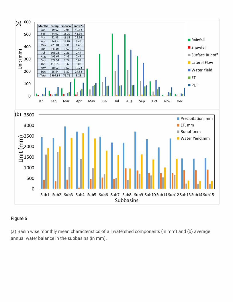
Figure 6

(a) Basin wise monthly mean characteristics of all watershed components (in mm) and (b) averageannual water balance in the subbasins (in mm).

Figure 7

(a) Observed, raw and bias-corrected temperature at Taplejung station and (b) Observed, raw and bias-corrected precipitation at the Taplejung station.

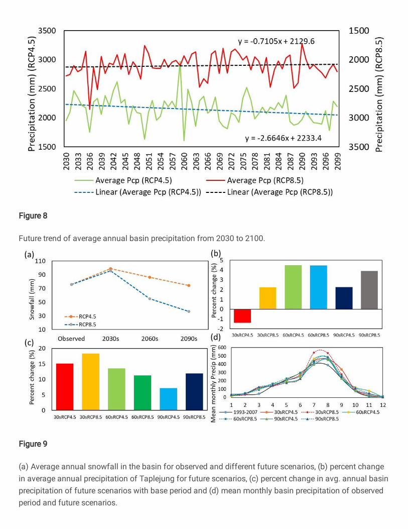
Figure 8

Future trend of average annual basin precipitation from 2030 to 2100.

Figure 9

(a) Average annual snowfall in the basin for observed and different future scenarios, (b) percent changein average annual precipitation of Taplejung for future scenarios, (c) percent change in avg. annual basinprecipitation of future scenarios with base period and (d) mean monthly basin precipitation of observedperiod and future scenarios.

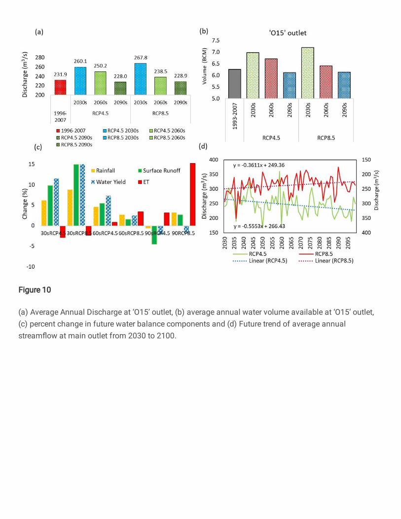
Figure 10

(a) Average Annual Discharge at ‘O15’ outlet, (b) average annual water volume available at ‘O15’ outlet,(c) percent change in future water balance components and (d) Future trend of average annualstream�ow at main outlet from 2030 to 2100.

Figure 11

Monthly average stream�ow of base period & different future scenarios.

Figure 12

(a) Month-wise FDCs for the baseline period (1996-2007) and (b) FDC (on daily �ow) of baseline periodand under future scenarios.

Figure 13

Percentile monthly �ow at Majhitar outlet for observed and future scenarios.

assessment of historical and future water availability in

Documents