2005-ETT-003 Grin 1

Assessment of LNG Transport Chains Using Weather-Based Voyage Simulations

Rob Grin (V), Jaap de Wilde (V) and Jos van Doorn (V) Maritime Research Institute Netherlands

ABSTRACT

It is well known that the weather can have considerable effects on the delivery reliability of an LNG supply chain. These effects will become even more important when the receiving terminal is located offshore. Presently most operability studies consider the transport and offloading independently and do not account for the coherence between the subsequent transport chain stages. This paper presents a realistic example and shows the extensive capabilities of the newly proposed combined approach. This approach consists of a complete simulation of the LNG transport chain and accounts for the offloading operation as well.

KEY WORDS: LNG; operability; downtime; simulation; offloading; weather; FSRU. INTRODUCTION Traditionally LNG transportation has a special position in the maritime transportation sector. Not only because of its long term charter contracts, its relatively small fleet or its cryogenic cargo contents, but also because it is part of a closely fitting logistic chain which puts high demands on delivery reliability. For that reason, additional attention is not only paid to the performance of the transport chain stages itself but also to their interaction. However, it has always been difficult to incorporate the effect of environmental conditions in these evaluations. The Maritime Research Institute Netherlands (MARIN) has developed a new generation of scenario simulation tools that account for the weather effects in a detailed and realistic way. In the simulations the voyages and offloading operation are stepwise evaluated. This makes it possible to fully account for the weather effects on delivery reliability. The study focuses on the transport of the LNG because this part of the LNG chain, in particular, may be seriously affected by weather. The total LNG chain consists of several successive stages where each stage is dependent on the preceding stage. For that reason, the environmental conditions during transport affect the overall reliability of delivery. It is expected that overall US gas demand will increase by about 40% in the coming decades. The US domestic natural gas production and Canadian pipeline imports are most likely not able to meet this increasing demand. For that reason, it is expected that LNG imports will increase significantly over the coming years. The capacity of the currently operational import terminals is not sufficient to meet future requirements, and therefore several new import terminals are proposed. The public concerns about the safety of transportation and storage of LNG is one of the most important reasons that many of the proposed terminals are located offshore.

In the presented example, LNG will be imported from Qatar to a floating storage and regasification unit (FSRU) on the US Northeast Coast. This case is selected for the following reasons: − Qatar’s gas reserves are on the order of 15% of the total

global proven gas reserves, and it is likely that the export to the USA will increase, even after considering the longer distance when compared to such LNG producers as Trinidad and Tobago or Algeria.

− The Suez Canal introduces an extra dimension to the transport simulations because the Suez Canal can be passed only once a day.

− The weather conditions on the transatlantic passage impose restrictions on the sustained speed, especially during winter.

− The offloading site is quite exposed, and therefore the offloading operation cannot be started in all weather conditions.

The presented transport chain is an example to show the sometimes complex weather effects on LNG transportation. For that reason, the loading operation at Qatar and the Suez Canal passage, which are hardly affected by the weather, have a fixed duration. The voyage simulations account for the recovery of weather delays obtained during the voyage itself, as well as delays obtained during the offloading operation. On arrival at the offloading site, the offloading operation is only started if the weather forecast is good enough to permit completion of the offloading operation. If the forecast calls for unacceptable weather, offloading is delayed until the first appropriate weather window. The transports will be performed with three LNG carriers, arriving at the FSRU in a 13-day cycle. Consequently, terminal congestion due to berth availability is not a significant issue. It is evident that an actual project will be more complex; however the approach would be similar and refinements could easily be implemented. The delivery reliability and operational costs are the main results of the scenario simulation approach. Together with the capital cost of the LNG carriers and offloading terminal, it will provide a solid basis for the selection of the most profitable alternative when various transport options are available.

2005-ETT-003 Grin 2

Qatar (24 hrs)

− Spare time (2 hrs)− Approach and berthing (2 hrs)− Loading (18 hrs)−Unberthing and departure (2 hrs)

Suez Canal (22 hrs)

− Spare time (2 hrs)− Anchor (5 hrs)− Passage (14 hrs)

Suez Canal (23 hrs)

− Spare time (2 hrs)− Anchor (5 hrs)− Passage (16 hrs)

Offloading (21 hrs)

− Approach and berthing (2 hrs)− Offloading (18 hrs)−Unberthing and departure (1 hrs)

Arrival at waiting area (minimal 2 hrs)

− Spare time (2 hrs)− Waiting for weather window( )

Transit (159.5 hrs)18.6 knots

Transit (159.5 hrs)18.6 knots

Round-trip schedule− Total distance: 15,800 nm− Total duration: 936 hrs− Total fuel costs: $0.49M

Transit (263.0 hrs)18.5 knots

Transit (263.0 hrs)18.5 knots

Figure 1. Transport chain Qatar – Northeast US coast SCHEDULE TRANSPORT CHAIN The transport chain that is adopted between Qatar and the Northeast US coast is given in Figure 1. The total round-trip time is 39 days. The scenario simulations, which model the transport chain, consist of two parts: − The main program which describes the transport chain. It

controls the round trips, the stages with a fixed duration and the way in which delays are recovered.

− Voyage simulations in Figure 1 are denoted by the arrows containing transit time and speed (more details are given in the following chapter “Applied Techniques”).

A total of 108 round trips were simulated per LNG carrier with each round trip split up into 4 strings of 27 subsequent round trips. The difference between the start dates of each string is 3 days in order to ensure that the weather conditions were independent between the strings. By coupling subsequent round trips to strings, it was possible to determine the transport capacity, fuel consumption, and the system’s ability to recover delays. Qatar The round trip starts at Qatar, where the LNG carrier is loaded. The net loading time is typically about 12 hours. Together with the connection and pre-cooling of the loading arms and, after loading, heating and disconnection of the loading arms, the total loading operation takes 18 hours. Deberthing, departure and disembarking the pilot takes 2 hours. The loading operation at Qatar has a fixed duration in the simulations because it is assumed that the weather effects are negligible. This stage is controlled by the main program.

Qatar to Suez The approximately 2960 nm voyage from Qatar to Suez takes 159.5 hours at a speed of 18.6 knots. The maximum speed at 90% MCR (maximum continuous rating) is almost 21 knots. Accordingly, it is possible recover delays up to 12 hours without missing the daily slot for the Suez Canal. This margin will be used when delayed ships try to get back on schedule. This part of the round trip is controlled by the voyage simulator. Suez Canal passage The route is cut in two by the Suez Canal which introduces two additional fixed arrival times. Arriving late at Suez or Port Said causes at best a considerable surcharge or at worst a day’s delay because there is only one daily departure from each side of the canal. Two hours spare time is incorporated in the schedule in order to have some margin before a surcharge has to be paid. This surcharge could be substantial and has a maximum of $20,000. The total passage time, including spare time and anchorage, is 22 hours and is considered to be invariable in the simulations. This stage is controlled by the main program. Port Said to Northeast US coast After the Suez Canal passage, the voyage to the US Northeast coast is made. The distance of this voyage is about 4850 nm and has a duration of almost 11 days at a speed of 18.5 knots. Up to 24 hours delay can be recovered on this leg when the weather conditions are favorable. This stage is controlled by the voyage simulator. Arrival at waiting area After arrival at the waiting area near the offloading site, the LNG carrier waits until the weather conditions are good enough for the subsequent 21 hours (the so-called “weather window”) to complete the offloading operation in one attempt. The limiting

2005-ETT-003 Grin 3

weather conditions are determined with fast-time maneuvering simulations and offloading simulations (both techniques are described in more detail in the chapter “Applied Techniques”). This stage is controlled by the main program. Offloading operation When the weather window is at least 21 hours long, the offloading operation is started. The operation consists of the approach and berthing (2 hrs), offloading (18 hrs) and deberthing and departure (1 hr). This stage is controlled by the main program. Return voyage The return voyage consists of the voyage from the offloading site to Port Said, the Suez Canal passage and the voyage to Qatar. The procedure followed during those stages is equal to the aforementioned stages. Offloading Site and FSRU The offloading site is located at a realistic location about 30 nm from the US Northeast coast at a water depth of almost 50 meters. The location of the offshore site means that the FSRU will experience almost fully exposed environments from the Atlantic Ocean. Actual floating LNG terminals will probably be located in more sheltered areas to avoid dealing with overly harsh environments. However, the chosen offshore locations have the advantage of being far out of sight from the coast and outside the main coastal traffic routes. A generic floating LNG terminal is considered in this paper. The FSRU receives regular shipments of LNG from LNG carriers, transfers them to the onboard storage tanks, and regasifies the LNG for transport to shore. The terminal has the capacity to import significant volumes of clean dry natural gas for the Northeast coast of the US. The FSRU is designed as a large barge that is permanently moored on station and free to weathervane about a single point mooring (SPM). Loading LNG into the FSRU from the LNG carriers is done via four loading arms (three liquid arms and one vapor arm). The storage capacity of the unit is 270,000 m³.

Figure 2. Location offloading site and computational domain of local wind-wave model

In general, the free weathervaning system finds an equilibrium heading in the combined wind, wave and current forces. In our case, the maximum of 1 knot current is considered small compared to the wind and wave forces. Because of the large wind area, it is assumed that the system heads into the wind. In other words, the relative wave angle equals the angle between the wind and the waves. In case of high cross current speeds, the use of a thruster at the stern of the FSRU may be considered to give the system a more favorable heading. However, a passive system is considered in this paper. LNG Carrier Design It is chosen to evaluate a conventional membrane type LNG carrier with a nominal cargo capacity of 145,000 m³. The main dimensions of the vessel are given in Table 1. Table 1. Main dimensions of LNG carrier

Length over all [m] 286.00 Length perpendiculars [m] 274.00 Breadth [m] 43.35 Depth to main deck [m] 26.00 Draft [m] 11.38 Deadweight [tonnes] 71,809 Gross tonnage [tonnes] 98,261 Displacement [m³] 102,170 Cargo capacity [m³] 145,000

In contrast to most existing LNG carriers, the design is not equipped with a steam turbine but is equipped with a 2-stroke diesel engine in combination with a reliquefaction plant. This configuration has the advantage of higher fuel efficiency and preservation of the boil-off during the long voyages and potential offloading delays. However, it will require significant energy to reliquefy the boil-off. The main engine has a nominal output of 31 MW at 76 RPM. As a first estimate, the specific fuel oil consumption is assumed to be constant at a given torque which is shown in Figure 3. Furthermore, the operational envelope of the main engine is also given in the figure. Within that envelope, the engine can run continuously without overloading.

0

10

20

30

40 50 60 70 80Revolutions [RPM]

Bra

ke

po

wer

[MW

]

175.1 g/kWh

190.5 g/kWh

179.2 g/kWh

Figure 3. Lines of constant specific fuel consumption

2005-ETT-003 Grin 4

APPLIED TECHNIQUES Voyage Simulation Techniques The voyage simulations are part of the transport chain simulations. The voyage duration is the only variable which is required as input from the main program while the remaining input is established prior to the simulations. The output to the main program is the actual arrival time and fuel consumption, while all other output is stored in a separate database. In this chapter a general description of the voyage simulation tool GULLIVER (Dallinga, 2004) is given. A generalization of the calculation and decision logic is presented in Figure 4. User inputs to this simulation tool are shown on the left side of the figure and are described below: Environmental databases The environmental conditions consist of historic time records of wind (speed and direction), currents (speed and direction) and short-crested wave spectra. Short-crested wave spectra describe not only the distribution of the wave energy over the frequencies but also the distribution over the wave directions. Since waves are never coming from exactly one direction, this represents realistic sea conditions better. Furthermore, it enables the description of wind seas coming from directions other than the swell. The 2-dimensional spectra are read directly from a database or are reconstructed from wave parameters (wave height, period and direction) of wind sea and swell. Weather forecasts are not supplied to the voyage simulations. RAO database Operability studies focus primarily on operational conditions and less on extreme events. Accordingly, the ship behavior is expected to be fairly linear in character throughout most of the practical domain. Because of this and the large volume of calculations that underlies a meaningful workability study, conventional frequency domain tools (strip theory or 3D panel codes) are commonly used as a starting point for the generation of the RAO database. However, model tests are still the most reliable way to determine ship behavior and will improve the reliability of the prediction considerably. In particular, the added resistance, roll damping, slamming, sloshing and behavior in stern quartering waves are difficult to assess numerically. Operational scenario The flexibility for setting up operational scenarios is large and can be divided into the following three items: − Seakeeping criteria These criteria describe the limiting conditions with respect to

comfort (e.g. motion sickness incidence, motion induced interruptions) and safety (e.g. lashing loads, shipping water, slamming, bending moment). When one or more criteria are exceeded, speed is reduced. This is called ‘voluntary’ speed

reduction. It must be noted that weather routing is not taken into account in the simulations.

− Engine settings The following engine settings can be chosen: constant

power, constant torque or constant revolutions. Secondly, the engine limitations are set. The involuntary speed loss originates from the chosen engine setting, the resistance and propulsion characteristics.

− Arrival time requirements

The arrival time depends on the occurrence of ‘voluntary’ speed reduction and/or involuntary speed loss. Basically three options are available. The first option is a ‘just in time’ scenario where ships try to recover delays in order to arrive at the scheduled time. The second option is constant speed. In this scenario speed is maintained but delays are not recovered. The third scenario is constant engine setting, where the selected engine setting (constant power, torque or revolutions) is maintained and delays are not recovered.

criteria satisfied

?

adapt sustained speed

get local environment

calculate behaviour

update ship position

destination

reached ?

stop

yes

no

no

yes

start: set initial position

scenario

RAO database

environment databases

calculate sustained speed

Figure 4. Flow chart of one voyage simulation Calculation and decision logic The voyage is step-wise simulated which is shown in the figure’s middle column. First, the local weather conditions are obtained from the environmental time records. Based on the weather conditions, the sustained speed is calculated accounting for the added resistance, main engine limitations and required arrival time.

2005-ETT-003 Grin 5

When the speed is known, the behavior of the ship is determined in such terms as roll motions, vertical accelerations, shipping water and comfort. Subsequently the behavior is compared to the predefined criteria. When one or more criteria are exceeded, speed is reduced until the criteria are met or the lower power limit of the main engine is reached (inner loop in the flow diagram). As soon as the new sustained speed is known, the new ship position is calculated. If the destination is not reached, the simulation model initiates the next voyage time-step. If the destination is reached, all results are stored and the trip duration and fuel consumption are returned to the main program. Applied Scenario during Voyages Reliability is essential in LNG shipping, and for this reason a ‘Just In Time’ (JIT) scenario including ‘voluntary’ speed reduction is adopted. In this scenario, the ship tries to maintain the scheduled arrival time. Delays, caused by involuntary speed loss or voluntary speed reduction, are recovered during the same voyage when possible. Involuntary speed loss denotes the speed loss due to a higher power demand in wind and waves than can be delivered by the main engine. ‘Voluntary’ speed reduction denotes speed reduction by the crew due to intolerable ship behavior. In the simulations, the relative velocity at the bow is the only criterion from which it is effectively decided to reduce speed. The relative velocity at the bow is a good measure for the probability of keel slamming as well as bow flare slamming. A threshold value of 9.0 m/s is adopted. Not more than 90% MCR is allowed and the minimum allowable engine load is 30% MCR. The selected engine mode is constant torque. A more complex scenario is required to recover the sometimes substantial delays occurred during offloading due to the passage constraints at the Suez Canal. For example when the delay is 30 hours after offloading, the delay is recovered in the following way. On the return trip to Suez Canal, only 6 hours is recoverable. Recovering more than 6 hours is not beneficial because it results in a long fuel-inefficient waiting time at Port Said (catching up 30 hours is not possible because it requires an average speed of 20.8 knots). On the ballast trip to Qatar and the loaded trip from Qatar the remaining delay of 24 hrs is equally recovered arriving at Suez exactly at the scheduled time. Approach and (Un)berthing Techniques To determine the maximum conditions under which an approach can be made to the FSRU, maneuvering simulations were done with a fast-time simulation model (van Doorn 2002). These simulations were made prior to the transport chain simulations.

The result of the series of fast-time simulations is a matrix of environmental conditions under which the approach and (de)berthing is allowed. This weather window is the input for the transport chain simulations. The set-up and mathematical content of a fast-time or real-time simulation model is practically equal. The main difference between the two models is that the real-time model is steered by a human being and the fast-time model is controlled by an autopilot. The principle set-up of a fast-time model is shown in the next figure.

SimulationControl

SimulatorManager

ScenarioHandler

- Select scenario

- Select condition

- Start

- Stop

- Normal procedues(approach speed;

course;autopilot settings)

- Emergency

- Emergency respons

Environment

- Waves

- Wind

- Current

Export

tanker FPSO

- Math.model

- Autopilotsettings

Tugs

- Tug assistcapabilities

Lines

- Hawser

- Mooringsystem

(Fast-time) Simulator

Results

- Trackplots

- Dataplots

- Statistics

- Collision data

(Auto) Pilot

Figure 5. Set-up of a (fast-time) simulation model In this figure the following blocks can be distinguished: − Input parameters (Environment, Vessels, Tugs, Lines) − Simulation model (Pilot and (Fast-time) Simulator) The mooring master and tug masters in the real-time simulation model are replaced by an autopilot in the fast-time simulation model. This autopilot controls the ship, responds to emergencies and orders the tugboats. The response of the autopilot is not equal to the response of a human. However, it has the advantage of consistent reactions which makes the results of the simulations comparable. The autopilot generally performs better than a human navigator. Consequently, the result of the simulation can be regarded as the “best possible”. This means that in the analysis of the results safety margins have to be built in to make sure that the human is capable of doing the maneuver. Modeling Before simulations can be executed the input parameters, such as the environmental conditions, ship characteristics and tugs, have to be modeled. The ship maneuvering behavior is an important aspect in the simulation. The technique to develop mathematical maneuvering models is based on a combination of model tests and full-scale sea trials. Added to the maneuvering model are the environmental forces resulting from waves and wind and

2005-ETT-003 Grin 6

engine characteristics. When the vessels are working in close proximity, the local shielding effects, especially on wind and current, have to be taken into account. One of the aims of the nautical study is to define the required tugboat power and type. In the end, the tugs are required to provide a certain force to keep the vessel under control. In the fast-time simulation model, tugs are modeled as tug capability diagrams. These diagrams show the effective pulling or pushing force as a function of: bollard position on the tanker, pulling or pushing angle, ship speed and wave height. Furthermore, the modeling of the tugs has to take into account the maximum speed for tugs to change position while assisting a large tanker. This response time is dependent on the line length and the tug type. Results of simulations The results of (individual) simulations are presented as plots showing the track of the vessel. Furthermore, a number of data plots are prepared showing the ship speed, rudder use, engine use and tug forces as function of the sailed track. In Figure 6 and Figure 7 an example is presented of a LNG carrier approaching a turret moored FSRU, as it prepares for berthing alongside. Whether a run is acceptable or not, depends on the ship speed at critical distances, the amount of engine power used, the rudder use and tug use. In general it is required to have sufficient spare maneuvering power available to be able to respond to emergency cases. Consequently, rudder, engine and tug power should not be used to the maximum.

-800

-600

-400

-200

0

1000 1100 1200 1300 1400 1500 1600

X-F

orce

ster

n tu

g [k

N]

-600

-300

0

300

600

1000 1100 1200 1300 1400 1500 1600

Y-F

orce

ster

n tu

g [k

N]

Figure 6. Tug forces as function of the sailed track (stern tug) For the approach to, and the departure from, the FSRU a series of fast-time simulations have been executed under various weather conditions. In addition to normal approaches, emergency approaches were also included in the simulation program. The results of the simulations together with workability data of the tugs determine the bollard pull requirements and the weather window. It should be noted that the response in case of an emergency determines, to a large extent, the bollard pull requirements. For practical reasons (redundancy) a three tug configuration was selected. The bow tug with a bollard pull of 66 tons and the stern tugs of respectively 55 and 44 tons were selected.

Figure 7. Track plot of an approach to a turret moored FSRU Applied Scenario during Approach and Berthing A side-by-side offloading operation at the floating LNG terminal can be divided into the following steps: − Approach − Berthing − Fastening of mooring lines − Connecting the LNG loading arms − Offloading (18 hours) − Disconnection and departure (1 hour) After arrival at the designated waiting area located approximately 2 to 3 miles from the FSRU, the pilot boards and the vessel starts to make the approach to the FSRU. This approach can only start when the weather forecast indicates that the weather conditions (current, wind and waves) are good enough for approaching, berthing and offloading. In the present analysis it is assumed that the weather forecast is perfectly predicted up to one day ahead. For that reason, the offloading operation is not started until the weather window is long enough to complete the total operation (21 hours). Both the approach maneuver and offloading are limited by weather conditions with particular sensitivity to relative direction of wave, wind and current. The mooring master maneuvers the LNG carrier to a position where he can start to make the approach at a course parallel to the FSRU. He will try to avoid ‘collision’ courses with the FSRU, certainly within 500 meters from the FSRU. At approximately 1 mile from the FSRU, the tugs connect. In this example, it is assumed that the LNG carrier is equipped with a bow thruster. The vessel is assisted by three tugs. One tug at the stern controls ship speed while generally pulling astern. The other stern tug is used to control the heading and is either pushing or pulling sideways. The bow tug will be used to

(2 hours)

2005-ETT-003 Grin 7

control the position of the bow. It is assumed that the tugs are escort tugs capable of working in relatively high waves. The fast-time simulation shows that with this tug configuration the LNG carrier can be kept under control in waves up to 2.5 meters and in winds up to 13.5 m/s (26 knots). Offloading Techniques Like the fast-time maneuvering simulations, the offloading simulations were performed prior to the transport chain simulations. The matrix containing the limiting weather conditions is the only input for the transport chain simulation. Two-body time domain simulations were carried out for the assessment of the weather limits for the side-by-side mooring operation at the FSRU (Buchner, 2001). The offloading LNG tanker was moored alongside the FSRU with 16 mooring lines and 4 large fenders at the waterline. The FSRU was free weathervaning on a turret at the bow. The mooring line loads, fender loads and relative motions between the two vessels were calculated in wind, wave and current conditions. A systematic series of wave heights and peak periods in the scatter diagram were run for establishing the weather limits for the side-by-side mooring operation. The batches consisted of 4 wave heights (Hs) by 6 peak periods (Tp), as shown in Figure 8. Each cell in the matrix represents a time domain simulation of a 3-hour irregular wave condition. The cells were given a red color (marked with an “X”) when the operation could not be carried out safely and green (marked with “OK”) otherwise. OCIMF safe working loads (SWL) were used as the criterion for the mooring line loads and the fender loads. For the cryogenic offloading arms, an operating envelope of 2 m in x, y and z direction was assumed as based on presently available technology. Batches with different angles between the wind, wave and current were carried out for determining the weather limits for non-parallel environments.

Hs [m]

4.0 X X X X OK

3.0 X X X OK OK

2.0 OK OK OK OK OK

1.0 OK OK OK OK OK

Tp [s] 6.0 10.0 14.0 18.0 22.0

Weather threshold

Figure 8. Weather limits for side-by-side mooring The hydrodynamics of the two vessels in very close proximity are very complex when considering the interactions of the wave forces, added mass, damping values and drift forces. The viscous damping of the surge, sway, yaw and roll motions of the two vessels close to each other is even more complex than for the vessels alone. The small distance between the vessels results in large local water velocities in the gap and around the bilges. Finally, there is a significant interaction for the wind and current forces.

A multiple-body time domain simulation requires the following steps: − A multiple-body diffraction analysis in the frequency

domain. − Preparation of the hydrostatic terms of all bodies. − Calculation of the retardation functions in the time domain. − Preparation of the stiffness, damping and friction effects of

the mooring system. − Calculation of the time traces of the wave forces and the low

frequency drift forces in a certain realization of the wave spectrum.

− Performance and analysis of the simulation in the time domain.

Diffraction analysis The wave forces, added mass, damping and drift forces of the two vessels were calculated with the linear diffraction analysis tool DIFFRAC. The panel distribution for the side-by-side configuration is depicted in Figure 9. A free surface lid was placed on the gap between the FSRU and the alongside moored carrier in order to suppress unrealistic local wave behavior in the diffraction analysis. (Huijsmans, 2001).

Figure 9. Panel distribution of LNG tanker alongside a barge- type FSRU Time domain simulations The time domain program LIFSIM was initially developed for the numerical simulation of offshore lifting operations. It is able to simulate the interaction between (up to) three floating bodies, related to their mooring system and their hydrodynamic interactions. LIFSIM integrates the linear equation of motions for the FSRU and the LNG tanker while taking into account the inertia forces, wave loads, damping loads and hydrostatic restoring forces. The mooring systems are modeled with their (non-linear) quasi-static force deflection characteristic. The Coulomb friction of the floating fenders between the two vessels is calculated at each time step. The model can handle slack line situations and situations where the LNG tanker gets free from the fenders. Applied Scenario during Offloading The weather limits for the LNG offloading in this paper are based on existing time domain offloading simulations of the side-by-side concept for similar type FSRU’s and environments. The following four criteria were used in the transport

2005-ETT-003 Grin 8

simulations (see Figure 10). The limiting lines were derived as a polynomial fit through previously calculated red-green tables, as shown in Figure 8. − If the angle between the wind and the waves is within 15

degrees, use the 15 degree curve. − If the angle between the wind and the waves is between 15

and 30 degrees, use the 30 degree curve. − If the angle between the wind and the waves is between 30

and 45 degrees, use the 45 degree curve. − If the angle between the wind and the waves is more than 45

degrees, use the “rest” curve.

0.0

1.0

2.0

3.0

4.0

5.0

0 4 8 12 16 20 24

Tp [s]

Hs

[m]

Rest

15°

45°30°

Figure 10. Weather limits for side-by-side offloading RESULTS AND DISCUSSION Environmental Conditions during Transit In the presented example, a three year database containing wind, wave and current data is applied. This time span is considered to be too short to be representative for the climate on the route but is sufficient to demonstrate the principle. For operability studies a period of at least 5 to 10 years is recommended to be sure that the climate description is complete and is not accidentally biased by either very calm or extreme years. The wind and wave data is obtained from the European Centre of Medium range Weather Forecasts (ECMWF) and consists of wind speed and direction and significant wave height, mean period and mean direction of wind sea and swell.

0.0

1.0

2.0

3.0

4.0

jan mar may jul sep nov

Wav

e he

ight

[m]

0

90

180

270

360

Dire

ctio

n [°

]

Wave height Wind directionWave direction

Figure 11. Monthly averages of wave height in [m] and average wind and wave direction in [°] on the Qatar – Suez Canal leg

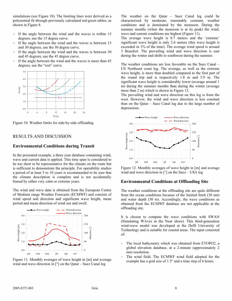
The weather on the Qatar – Suez Canal leg could be characterized by moderate, reasonably constant, weather conditions and is dominated by the monsoon. During the summer months (when the monsoon is at its peak) the wind, wave and current conditions are highest (Figure 11). The average wave height is 0.7 meters and the ‘extreme’ significant wave height is only 2.6 meters (this wave height is exceeded in 1% of the time). The average wind speed is around 3 Beaufort. The prevailing wind and wave direction is east during the winter and shifts to southwest during the summer. The weather conditions are less favorable on the Suez Canal – US Northeast coast leg. The average, as well as the extreme wave height, is more than doubled compared to the first part of the round trip and is respectively 1.8 m and 5.9 m. The significant wave height is considerably lower (average around 1 m) during the summer months than during the winter (average more than 2 m) which is shown in Figure 12. The prevailing wind and wave direction on this leg is from the west. However, the wind and wave direction is less constant than on the Qatar – Suez Canal leg due to the large number of depressions.

0.0

1.0

2.0

3.0

4.0

jan mar may jul sep nov

Wav

e he

ight

[m]

0

90

180

270

360

Dire

ctio

n [°

]

Wave height Wave directionWind direction

Figure 12. Monthly averages of wave height in [m] and average wind and wave direction in [°] on the Suez – USA leg Environmental Conditions at Offloading Site The weather conditions at the offloading site are quite different from the ocean conditions because of the limited fetch (30 nm) and water depth (50 m). Accordingly, the wave conditions as obtained from the ECMWF database are not applicable at the offloading site. It is chosen to compute the wave conditions with SWAN (Simulating WAves in the Near shore). This third-generation wind-wave model was developed at the Delft University of Technology and is suitable for coastal areas. The input consisted of: − The local bathymetry which was obtained from ETOPO2, a

global elevation database, at a 2-minute (approximately 2 nm) resolution.

− The wind field. The ECMWF wind field adopted for the example has a grid size of 1.5° and a time step of 6 hours.

2005-ETT-003 Grin 9

− The incoming swell at the southern and eastern boundary. The swell component given in the ECMWF database is used at these boundaries.

The computational domain ranges from 43°30΄N to 45°0΄N latitude and 70°30΄W to 68°0΄W longitude (see Figure 2). The tidal streams are not very strong at the offloading site (less than 1 knot) and are not considered in the presented example. As shown in Figure 13 the average wave height is around 1 m during summer increasing to around 1.5 m during winter. The ‘extreme’ wave height is 3.7 m (exceeded in 1% of the time). Notable is the large deviation between the average wind and wave direction. During winter, the average difference is around 90 degrees with the winds coming from the west and the waves coming from the south. This difference can be explained by the fact that the southerly swell coming from the Atlantic Ocean dominates the fetch limited seas originating from the wind coming from the land.

0.0

1.0

2.0

3.0

4.0

jan mar may jul sep nov

Wav

e he

ight

[m]

0

90

180

270

360

Dire

ctio

n [°

]

Wave height Wave directionWind direction

Figure 13. Monthly averages of wave height in [m] and average wind and wave direction in [°] at offloading site Voyage Results Round-trip duration One of the most basic results is the round-trip duration as shown in Figure 14. In only 75% of the round trips the duration is equal to the scheduled 39 days. The remaining 25% consists of round trips where (long) waiting times appeared before offloading and, as a consequence, round trips where it is tried to recover the imposed delays.

37 days, 2.2%

37.5 days, 3.4%

38 days, 0.6%

38.5 days, 6.5%

39.5 days, 7.1%

40 days, 0.9%

40.5 days, 1.5%

≥41 days, 2.5%

Other,24.7%39 days,

75.3%

Figure 14. Distribution of round-trip duration in days

The longest delay was 4.5 days. It took 3 round trips to recover this delay completely because additional delays occurred during the subsequent round trips. In the ideal case, the delay would have been recovered during the return voyage to Qatar (1.5 days) with the remainder recovered on the subsequent round trip (3 days). The scenario allows for a maximum recovery of 3 days (two times 24 hours and two times 12 hours). Fortunately a three day recovery was never required because it would have caused a substantial increase in the fuel costs. However, the highest recovered delay was still two days, this occurred 7 times (2.2%), and required also a considerable amount of additional fuel. More details about the fuel consumption will be discussed at the end of this section. In Table 2 the deviation from the scheduled voyage duration is shown for the four separate legs. In 84% of the voyages from Qatar to Suez Canal and vice versa, the trip duration is equal to the schedule. The remaining 16% of the voyages were 12 hrs shorter than scheduled (no delays were observed). As explained in the operational scenario, delays are recovered on subsequent voyages. Long delays can only be recovered in discrete steps of 24 hours due to the Suez Canal. In case of the Suez Canal – Qatar route this results in a recoverable delay of 12 hrs on the return voyage and again 12 hours on the loaded voyage to Suez. 80% of the voyages from the Suez Canal to the offloading site have the scheduled duration of 263 hours. This is the only leg where delays were observed (14%). Table 2. Distribution of deviation from scheduled voyage duration in hours per leg

∆t [hrs]

Qatar to

Suez

Suez to

USA

USA to

Suez

Suez to

Qatar -27 to -21 0% 2% 6% 0% -21 to -15 0% 3% 6% 0% -15 to -9 16% 1% 10% 16% -9 to -3 0% 1% 14% 0%

Scheduled 84% 80% 64% 84% +3 to +9 0% 7% 0% 0%

+9 to +15 0% 1% 0% 0% +15 to +21 0% 2% 0% 0%

+21 > 0% 4% 0% 0% Although the voyages to the USA were the most demanding voyages due to a high fraction of westerly winds and waves, it was possible to (partially) recover delays in 7% of the voyages. In all cases, it was tried to recover delays of 24 hours but succeeded in only 2% of the voyages. The return trips from the offloading site show a high fraction of voyages where delays were (partially) recovered, accounting for the fixed arrival time at Port Said.

2005-ETT-003 Grin 10

Storage volume FSRU [x 1000 m³]

0

100

200

300

Jan-97 Jul-97 Jan-98 Jul-98 Jan-99 Jul-99 Jan-00

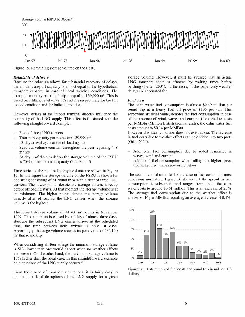
Figure 15. Remaining storage volume on the FSRU Reliability of delivery Because the schedule allows for substantial recovery of delays, the annual transport capacity is almost equal to the hypothetical transport capacity in case of ideal weather conditions. The transport capacity per round trip is equal to 139,900 m³. This is based on a filling level of 98.5% and 2% respectively for the full loaded condition and the ballast condition. However, delays at the import terminal directly influence the continuity of the LNG supply. This effect is illustrated with the following straightforward example; − Fleet of three LNG carriers − Transport capacity per round trip 139,900 m³ − 13-day arrival cycle at the offloading site − Send-out volume constant throughout the year, equaling 448

m³/hrs − At day 1 of the simulation the storage volume of the FSRU

is 75% of the nominal capacity (202,500 m³) Time series of the required storage volume are shown in Figure 15. In this figure the storage volume on the FSRU is shown for one string consisting of 81 round trips with a fleet of three LNG carriers. The lower points denote the storage volume directly before offloading starts. At that moment the storage volume is at its minimum. The higher points denote the storage volume directly after offloading the LNG carrier when the storage volume is the highest. The lowest storage volume of 34,800 m³ occurs in November 1997. This minimum is caused by a delay of almost three days. Because the subsequent LNG carrier arrives at the scheduled time, the time between both arrivals is only 10 days. Accordingly, the stage volume reaches its peak value of 232,100 m³ that round trip. When considering all four strings the minimum storage volume is 51% lower than one would expect when no weather effects are present. On the other hand, the maximum storage volume is 10% higher than the ideal case. In this straightforward example no disruptions of the LNG supply occurred. From these kind of transport simulations, it is fairly easy to obtain the risk of disruptions of the LNG supply for a given

storage volume. However, it must be stressed that an actual LNG transport chain is affected by waiting times before berthing (Hertel, 2004). Furthermore, in this paper only weather delays are accounted for. Fuel costs The calm water fuel consumption is almost $0.49 million per round trip at a heavy fuel oil price of $190 per ton. This somewhat artificial value, denotes the fuel consumption in case of the absence of wind, waves and current. Converted to costs per MMBtu (Million British thermal units), the calm water fuel costs amount to $0.14 per MMBtu. However this ideal condition does not exist at sea. The increase in fuel costs due to weather effects can be divided into two parts (Grin, 2004): − Additional fuel consumption due to added resistance in

waves, wind and current. − Additional fuel consumption when sailing at a higher speed

than scheduled while recovering delays. The second contribution to the increase in fuel costs is in most conditions normative. Figure 16 shows that the spread in fuel consumption is substantial and ranges from about the calm water costs to around $0.61 million. This is an increase of 25%. The average fuel consumption due to the weather effect is almost $0.16 per MMBtu, equaling an average increase of 8.4%.

2%

12%

15%

11%

14%

6% 6%

3%2% 2%

3%1%

23%

0%

5%

10%

15%

20%

25%

0.49 0.51 0.53 0.55 0.57 0.59 0.61

Figure 16. Distribution of fuel costs per round trip in million US dollars

2005-ETT-003 Grin 11

23-Nov

12:00

24-Nov

00:00

24-Nov

12:00

25-Nov

00:00

25-Nov

12:00

26-Nov

00:00

26-Nov

12:00

27-Nov

00:00

27-Nov

12:00

28-Nov

00:00

Wave direction [°]

Waiting Offloading Return voyage to QatarArrival

Downtime; offloading onlyDowntime; approach, (un)berthing and offloading

Figure 17. Example of a 30 hour delay in a November storm period

Approach, Berthing and Offloading Results The distribution of waiting times at the FSRU is presented in Figure 18. In over 90% of the events the waiting time is less than 1 day. In most cases there is no waiting time at all. The longest waiting time that occurred in our simulations was five days.

,

1.0 day, 5.3%

No waiting time, 75.3%

0.5 day, 9.6%

1.5 day, 4.3%, Other,9.9% 2 days, 2.5%

,

more than 2 days, 3.1%

, ,

Figure 18. Distribution of waiting times in days before offshore operation was possible

The relatively large number of waiting events at the offloading site can be explained by the almost fully exposed environments at the offshore site. A more sheltered location would improve the workability. Also the installation of a good heading control system on the FSRU would result in better up-time figures. An example of a 30 hour delay in a November storm period is presented in Figure 17. The LNG tanker arrives on November 23 at 19:50 hours. At that moment the conditions at the site would allow to start with the operation, but the weather forecast indicates deteriorating conditions, and it is decided to wait for a better window. The local waves exceeding 2 to 3 m significant in combination with the more than 20 knot (10 m/s) winds do not allow for a safe maneuver and subsequent offloading. It is also noted that the angle between the wind and the waves increases from almost parallel (180 degrees) to quartering waves (135 degrees) during the waiting period, which would have resulted in increasing vessel motions if the offloading would have been started. On November 25, the waves have calmed down to less than 2 m significant and the forecast indicates a good weather window for

2005-ETT-003 Grin 12

at least the next 24 hours. The approach and berthing operation is commenced and 21 hours later the operation is successfully completed. The empty carrier heads back to Qatar and will try to recover the lost time by sailing at an increased speed. Future Developments Several items are not covered in the present transport chain simulation, but will be investigated and, if necessary, developed in the (near) future. It is expected that these items increase the completeness and accuracy of the results. Some of these future developments are listed below: − Investigation of the effects of including weather forecasts

and weather routing in the voyage simulations. − Include the effects of queuing (terminal congestion because

the berth is not available). − Account for the effect of sloshing and the related interaction

with the vessel and FSRU motions when the cargo tanks are partially filled.

− Evaluation of the effects on the resistance of the vessel due to such issues as fouling, shallow water, seawater temperature, steering and drift angle.

− Research on the behavior and performance of tugs in waves. − Further development of the time domain side-by-side

offloading technique. Fundamental research is presently being carried out to describe the local wave behavior in the gap between the two vessels in a more realistic way.

CONCLUSIONS It has always been difficult to incorporate the effect of environmental conditions in LNG transport chain evaluations. Most operability studies account for the weather in a statistical way. A major drawback of this approach is the absence of possibilities to build on past and future conditions such as the recovery of delays. Additionally, most operability studies did not include interactions between the subsequent stages in the transport chain. In this paper a new combined approach is proposed, consisting of voyage simulations that account for the offloading operation as well. The paper deals only with weather delays, but more complicated scenarios, like fleet simulations, could be implemented easily. Regarding the presented example, the following conclusions can be drawn: − Large variations in voyage duration were found that resulted

from bad weather during the voyages and waiting times at the offloading site. The latter is normative, with the highest fraction and longest delays. In all cases it was possible to recover the lost time by sailing at an increased speed on the subsequent voyages and round trips.

− The speed increase to recover weather delays, requires up to 25% more fuel, with a proportional increase in emissions. The average increase in fuel consumption is 8.4% compared to the calm water consumption.

− In over 90% of the trips the waiting time at the floating terminal is less than 1 day. In 75.3% of the trips there is no waiting time at all. The relatively large number of waiting events at the floating terminal can be largely explained by the chosen location of the offloading site with almost fully exposed weather conditions.

− The delivery reliability is high, although during the winter large variations in storage volume occur. In one case the storage volume was 51% lower than one would expect when no weather effects are taken into account.

The example presented in this paper shows just a few applications of combined scenario simulations. This approach is especially suitable for the selection of the best alternative (e.g. ship design, propulsion options, schedule, route, offloading site, and offloading system). It gives the opportunity to evaluate the alternatives in terms of operational costs and delivery reliability accounting for the weather effects and interaction between the different stages in the transport chain. Transport chain simulations will provide a solid basis for the selection of the most profitable alternative when various transport options are available. REFERENCES BUCHNER, B., A.W. van DIJK and J.J. de WILDE.

“Numerical Multiple-Body Simulations of Side-by-Side Mooring to an FPSO.” ISOPE 2001 (Stavanger, 2001).

DALLINGA R.P. et al, “Scenario Simulations in Design for

Service.” PRADS 2004 (Lubeck-Travemunde, 2004). DOORN, J.T.M van and D. ten Hove. “F(P)SO Offloading

Concepts, their Nautical Feasibility and Safety Assessment.” OTC (Houston, 2002).

GRIN, R. and E. van de VOORDE. “Weather-Related

Economics of Natural Gas Transport for Two Propulsion Plant Configurations.” RINA Conference, Design and Operation of Gas Carriers (London, 2004).

HERTEL, M.L. and K.J. KINPORTS. “Using Simulation

Programs to Design and Analyze Marine Transportation Systems.” SNAME 2004 (Washington, 2004).

HUIJSMANS, R.H.M. et al. “Diffraction and Radiation of Waves around Side-by-Side Moored Vessels.” ISOPE 2001 (Stavanger, 2001).