assessment of marketed and marketable surplus of foodgrain crops … · assessment of marketed and...
TRANSCRIPT
ASSESSMENT OF MARKETED AND MARKETABLE SURPLUS OF
FOODGRAIN CROPS IN KARNATAKA
PARMOD KUMAR
ELUMALAI KANNAN
ROHI CHAUDHARY
KEDAR VISHNU
Agricultural Development and Rural Transformation Centre
Institute for Social and Economic Change
Bangalore- 560 072
December 2013

i
ASSESSMENT OF MARKETED AND MARKETABLE
SURPLUS OF FOODGRAIN CROPS IN KARNATAKA
PARMOD KUMAR
ELUMALAI KANNAN ROHI CHAUDHARY
KEDAR VISHNU
Agricultural Development and Rural Transformation Centre Institute for Social and Economic Change
Bangalore- 560 072
December 2013

ii
CONTENTS
Contents II-VI
Acknowledgements VII
Chapter I Introduction 1-14
1.1 Macro Overview of State Agriculture 1
1.2 Concept of Marketed and Marketable Surplus 2
1.2.1 Relationship between Marketed and Marketable Surplus 4
1.2.2 Factors Affecting Marketable Surplus and Marketed Surplus 4
1.3 Literature Review on Marketed and Marketable Surplus 5
1.4 Relevance of the Study 13
1.5 Objectives of the Study 14
1.6 Overview 14
Chapter II Coverage, Sampling Design and Methodology 15-18
2.1 Coverage and Sampling Design 15
2.2 Conceptual Framework and Theoretical Model of Marketed
Surplus
17
Chapter III Overview of Foodgrains Economy of Karnataka 19-45
3.1 Structural Transformation of the State Economy: Changing
Sectoral Shares
19
3.2 Cropping Pattern and Composition of Value of Output from
Agriculture
21
3.3 Growth Pattern of Area, Production and Yield of Major Crops 24
3.4 Growth Rates in Area, Production and Yield of Selected Crops,
District-wise
27
3.5 Marketed Surplus Ratios for Maize and Redgram in the state and
all India
31
3.6 Trends in Consumption of Major Inputs 34
Chapter IV Marketed and Marketable Surplus of Major Foodgrains In
Karnataka An Empirical Analysis
46-103
4.1 Main Features of Agriculture in Selected Districts 46
4.1.1 Geographical Features of Selected Districts 46
4.1.2 Socio-economic indicators of the selected districts 48
4.1.3 Classification of Workers 49
4.1.4 Land Utilization in the Selected Districts 49
4.1.5 Cropping Pattern in Selected Districts 54

iii
4.1.6 Macro Overview of Selected Districts 56
4.2 Main Features of Sample Households 57
4.2.1 Socio-economic Profile 57
4.2.2 Land Ownership Pattern/ Operational Holding Characteristics 60
4.2.3 Cropping Pattern and Physical Crop Productivity 62
4.2.4 Investment Pattern 66
4.3 Estimation of Crop Losses at Different Stages 68
4.3.1 Crop Loss on Farm (Harvesting, Threshing and Winnowing) 68
4.3.2 Crop Loss due to Transportation 71
4.3.3 Crop Loss during Storage 73
4.4 Estimation of Marketable and Marketed Surplus Ratios of
Selected Crop
76
4.4.1 Crop Wise Availability of Selected Crops by Farm Size 76
4.4.2 Crop Retention Pattern of selected Crops 77
4.4.3 Marketed and Marketable Surplus and Sale Pattern of Selected
Crops
79
4.5 Factors Affecting Marketed Surplus of Selected Crops 84
4.5.1 Socio- Economic Factors 84
4.5.2 Institutional Factors 84
4.5.3 Economic Factors 89
4.5.4 Infrastructural Factors 90
4.5.5 Technological Factors 93
4.6 Regression Results of Marketed and Marketable Surplus 95
4.7 Elasticity of Marketed Surplus to Total Output 98
Chapter V Concluding Observations and Policy Implications 100-105
5.1 Main Findings of the Study 100
5.1.1 Findings from Secondary Data 100
5.1.2 Findings from the Field Survey 102
5.2 Policy Implications 105
References 106-107

iv
LIST OF TABLES
Table No. Title Page No.
2.1 Details of selected household farmers - crop-wise 16
2.2 Details of sample households selected by Districts, Talukas and
Villages
17
3.1 Sectoral Shares to GSDP for Karnataka and India at 2004-05 prices 21
3.2 Contribution of various crops in total value of agricultural output at
2004-05 prices
22
3.3 Share of area under major crops in Karnataka & India 24
3.4 Growth rate of Area, Production and Yield of Major Crops in India 25
3.5 Growth Rate of area, production and yield of major crops in Karnataka 26
3.6.a District wise growth rates of area, production and yield for maize in
Karnataka
28
3.6.b District wise growth rates of Area, Production and Yield for Bengal
gram in Karnataka
30
3.6.c District wise growth rates of Area, Production and Yield for Redgram
in Karnataka
31
3.7 Marketed surplus ratio for maize and redgram in Karnataka and India 32
3.8 Percentage of area under HYV for maize in Karnataka and India 34
3.9 Percentage of irrigated area to cropped area for selected crops in
Karnataka and India
35
3.10 Consumption of NPK per hectare in Karnataka and India 37
3.11 Minimum Support Price for the selected crops 38
3.12 Paid out cost of selected crops in Karnataka (at 1999-00 Prices) 40
3.13 Agricultural credit (institutional) in Karnataka 40
3.14a Per 100 distribution of outstanding loan taken by farmers in
Karnataka
42
3.14b Per 100 distribution of outstanding loan taken by farmers in India 42
3.15 Farm mechanization – physical and financial estimates for 2012-13 43
4.1.1 Geographical area of selected districts 47
4.1.2 Topography of selected districts 47
4.1.3 Demographic profile of selected districts 48
4.1.4 Literacy rate of selected districts 49
4.1.5 Human Development Index and Gender Development Index for
selected districts
49
4.1.6 Classification of workers for selected districts 50
4.1.7a Land utilization of selected districts (hectares) during 2010-11 50
4.1.7b Land utilization (in percent to total geographical area) of selected
districts
51
4.1.8 Net sown area and GCA of selected districts 51
4.1.9a Source-wise net irrigated area of selected districts 52
4.1.9b Source-wise net irrigated area of selected districts (in percent) 53
4.1.10 District-wise actual rainfall for selected districts in Karnataka 53

v
4.1.11 District-wise area under principle crops in Karnataka during
(2010-11)
55
4.1.12 Share of agriculture and allied sector in GDDP 56
4.1.13 GDDP, NDDP, PCI and GSDP
57
4.2.1 Details of Selected Household 58
4.2.2 Households details district-wise 58
4.2.3 Characteristics of sampled population 59
4.2.4 Operational holding characteristics (per hectare) 61
4.2.5 Source of irrigation 61
4.2.6 Terms of leasing 62
4.2.7a Cropping pattern - area (hectares) 63
4.2.7b Cropping pattern - Percentage of gross cropped area 64
4.2.8 Crop wise yield observed by the selected farmers (kg/hectare) 65
4.2.9 Ownership of farm machinery by the selected households 67
4.2.10 Livestock ownership by selected farmers 67
4.2.11a Crop losses on farm - Bengalgram 69
4.2.11b Crop losses on farm - Maize 69
4.2.11c Crop losses on farm - Redgram 70
4.2.12a Crop losses during transportation - Bengalgram 71
4.2.12b Crop losses during transportation - Maize 72
4.2.12c Crop losses during transportation - Redgram 72
4.2.13a Crop losses due to storage at producer’s level - Bengalgram 74
4.2.13b Crop losses due to storage at producer’s level - Maize 74
4.2.13c Crop losses due to storage at producer’s level - Redgram 75
4.2.14 Crop wise availability of produce by farm size in (Quintals) 77
4.2.15 Crop retention pattern in quintal 78
4.2.16 Marketed and marketable surplus 80
4.2.17a Disposal of selected crops by place of sale - Bengalgram 82
4.2.17b Disposal of selected crops by place of sale - Maize 82
4.2.17c Disposal of selected crops by place of sale - Redgram 83
4.2.18 Source of price information for the selected crops 87
4.2.19 Credit by various sources according to the purpose 89
4.2.20 Policy awareness of farmers about the market existence 90
4.2.21 Disposal of marketed surplus according to the type of market 92
4.2.22 Distance and type of market 93
4.2.23 Area covered under improved seeds percent to total area under crop 94
4.2.24a Regression result on marketed surplus for redgram 96
4.2.24b Regression result on marketed surplus for maize 97
4.2.24c Regression result on marketed surplus for bengalgram 98
4.2.25 Elasticity of marketed surplus with respect to output 99

vi
LIST OF FIGURES
Figure No. Title Page
No.
2.1 District Map of Karnataka 18
3.1 Agricultural Map of Karnataka 19
3.1a Marketed Surplus Ratio Maize and Redgram in Karnataka 33
3.1b Marketed Surplus Ratio of Maize and Redgram in India 33
4.1 Actual rainfall distribution in selected districts of Karnataka 54

vii
ACKNOWLEDGEMENTS
The study was undertaken by the Agricultural Development and Rural Transformation Centre,
Institute for Social and Economic Change (ISEC) Bangalore on behest of Department of
Agriculture and Cooperation, Ministry of Agriculture, Government of India, New Delhi. The
study is a part of consolidated all India report being prepared by the Centre for Management in
Agriculture (CMA), Indian Institute of Management, Ahmedabad. The design of the study was
prepared by the CMA as also the questionnaire which we modified according to our requirement.
The team sincerely thanks Professor Vijay Paul Sharma for a well designed structure of the study
as well as providing all cooperation in undertaking this study. I sincerely thank the officials of
the Ministry for their cooperation and help.
The team sincerely thank our Director for his encouragement and constructive suggestions on the
project. The cooperation of ADRTC faculty and staff is duly acknowledged for their useful
comments and valuable suggestions on the questionnaire as well as their help in commencing the
field work. The team also wish to thank Mr. Arun Kumar and Mr. Kumar for their secretarial
help.
We appreciate the co-operation extended by the households in the primary survey and express
sincere thanks to all the respondents. The project team benefited from the interaction with
various Panchayat officials during the course of this study.
Ms. Prema helped in processing the data at different stages of the project and her contribution to
the report is acknowledged.
The report would have remained incomplete without the co-operation of all of them.

1
Chapter I
Introduction
1.1 Macro Overview of State Agriculture
Agriculture is an important part of economy of Karnataka state. The state has got a topography
that is highly suitable for agricultural activities. That is to say, Karnataka's relief, soil, climatic
conditions taken together contributes immensely towards growing various agricultural
commodities. Agriculture is one of the main occupations of the people in the state. About 12.31
million hectares of land, i.e., 64.6 percent of the total area is used for agriculture in Karnataka.
According to 2001 Census, about 71 percent of the workforce in Karnataka is farmers and
agricultural labourers. Agriculture of Karnataka is mainly dependent on monsoon, as only 26.6
percent of land is supported by irrigation. Agriculture in Karnataka can be classified into three
main seasons during the year, viz.:
Kharif (June to September)
Rabi (October to February) and
Summer (March to May)
Some of the important crops that form the basis of agriculture in Karnataka are: rice, jowar,
maize, pulses, oilseeds, cashew-nuts, coconut, arecanut, cardamom, chillies, cotton, sugarcane,
coffee, tobacco etc. Karnataka is the largest producer of coffee, coarse cereals and raw silk
among all states in India.Horticulture also plays a vital role in the economy of Karnataka. The
state is the major producer of horticultural commodities. About 40 percent of the total Income of
the state is generated from horticulture. Karnataka occupies the second position in terms of the
horticultural productions in India.
The agriculture and allied sector’s contribution to Karnataka’s GSDP was around 43 percent in
1980-81 that came down to 26 per cent in 2001-02 and further down to 16.8 percent during
2007-08 which remains stagnant at that level up to 2009-10. Despite the declining share of
primary sector in GSDP, agriculture remains the primary activity and main livelihood source for
the rural population in the state. Besides, agriculture provides raw material for a large number of
industries. Agriculture in the state is characterized by wide crop diversification. The extent of

2
arid land in Karnataka being second only to Rajasthan in the country, agriculture is highly
dependent on the vagaries of the southwest monsoon. The most important challenge faced by
agriculture in the state is food security, besides improving the livelihood of the farmers.
Karnataka has attained self sufficiency in food grains especially in the course cereals and pulses,
but still continues to be in deficit in rice and oilseeds (Kumar 2010). Development of agriculture
improves the purchasing power of the major section of our population, which in turn will also
help the development of other industries.
Karnataka also enjoys the credit of having pioneered organic farming policy before any other
Indian states. The state brought out an ‘Organic Farming Policy’ way back in March 2004.
Starting with small numbers, with a handful of farmers working on bringing about the change
almost a decade ago, today Karnataka has anywhere between 75 thousand hectares to 1.12 lakh
hectares of farming land producing organic crops and vegetables. Majority of this, nearly 51
thousand hectares has already been certified under organic cultivation. That is no mean feat, as it
takes close to three years to convert lands to organic from conventional farming methods.
The main objective of this policy was to increase food security and achieve
sustainability with the judicious use of precious land and water resources along with equipping
farmers to effectively mitigate the drought situation. The policy also aimed at enhancing soil
fertility and creating soil that was ‘living’. Further, this would be used to increase rural
employment and create opportunities for youth in the area, thereby checking migration while
making farmers self-dependent and also reducing the burden of debt.
Thus, it can be concluded that agriculture is an important part of the economy of Karnataka.
1.2 Concept of Marketed and Marketable Surplus
Marketing holds its origin from agriculture. It developed only after human beings learned to
produce more food needed for them. Few centuries ago farmers used to consume most of what
they produced and rest used to get distributed either as debt obligation or as wages to labourers.
But at later stages, farmers started producing to get required things by way of exchange; which in

3
turn boosted the importance of production. Since everything produced can neither be consumed
nor sold so emerged the concept of marketable and marketed Surplus.
Marketable Surplus
Marketable surplus is a theoretical concept which represents the surplus which the
farmer/producer has available with himself for disposal once the genuine requirements of the
farmer for family consumption, payment of wages in kind, feed, seed and wastage have been met
(Sadhu and Singh 2002, page 162). It is the portion of a harvest that a farmer can sell to the
market to earn a profit. With this profit he can reinvest into farming operations by purchasing
more land or better farming equipment or may save this profit or may use it to purchase personal
belongings. The term is also subjective in nature because the feature of retention of the farmer is
a matter of subjective guess. Marketable surplus may be defined objectively as the total quantity
of arrivals in the market out of the new crop.
Marketed Surplus
Another term that closely relates to marketable surplus is marketed surplus. It is more practical in
nature and refers to that part of the marketable surplus which is actually marketed by the
producer, i.e., not only the part which is available for disposal but the part which is actually
made available to the market or to the disposal of the non-farm rural and urban population. The
term is objective in nature, because it refers to the marketed amount, i.e., to the actual quantity
which enters the market (Kumar 2007).
In some cases, these terms may be interchangeable. The principal difference is time perspective:
marketable surplus is the produce that a farmer currently has on hand to take to market to earn a
profit, while marketed surplus is what he has already taken to the market to earn a profit. Both
marketed and marketable surplus have tremendous potential for ensuring prosperity in the
agricultural sector, because efficient marketing of the generated surplus can boost up capital
formation, real savings and real investment in the agricultural sector and ultimately raising the
welfare of the country as a whole. Also, if marketed surplus is satisfactory it can stop
unproductive migration from rural to the urban sectors, where people migrate in search of better
economic opportunities and petty jobs in towns and cities. Consequently, problems associated
with slum conditions of living could be reduced.

4
1.2.1 Relationship between Marketed and Marketable Surplus
The marketed surplus may be more, less or equal to the marketable surplus, depending upon the
condition of farmer and type of the crop.
a) Marketed Surplus > Marketable Surplus – this situation arises when the farmer retains
a smaller quantity of the crop than his actual requirement for family and farm needs. This
holds true especially for small and marginal farmers, whose need for cash is more urgent
and immediate. This situation of selling more than marketable surplus is termed as
distressed or forced sale. The quantity of distress sale increases with the fall in the price
of the product. A lower price means that a larger quantity will be sold to meet some fixed
cash requirement.
b) Marketed Surplus < Marketable Surplus – this occurs when the farmer retains some of
the surplus produce. The situation holds true under two conditions: First, large farmers
generally sell less than the marketable surplus because of their better retention capacity,
which is done in the hope of getting higher prices in later periods (at times up to the next
production season). Second, because of variation in prices farmers may substitute one
crop for another either for family consumption or for feeding their livestock. With the fall
in the price of the crop relative to a competing crop, the farmers may consume more of
the first and less of the second crop.
c) Marketed Surplus = Marketable Surplus – this occurs when farmer neither retains
more nor less than his requirement. This holds mostly true for perishable commodities.
1.2.2 Factors Affecting Marketable Surplus and Marketed Surplus
The Marketable Surplus differs from region to region, within the same region, and even from
crop to crop. Some of the factors affecting marketable surplus on a particular farm are:
i. Size of Holding: There is a positive relationship between the size of the holding and
marketable surplus.
ii. Production: The higher the production, the larger will be the marketable surplus.
iii. Price of the Commodity: There exists both positive and negative relation between both,
depending upon whether one considers short run or long run.

5
iv. Size of Family: There is a negative relationship between family size and marketable
surplus.
v. Requirement of Seed and Feed: The higher the requirement for seed and feed, the smaller
the marketable surplus.
vi. Nature of the Commodity: The marketable surplus of non-food crops is generally higher
than that of for food crops, as in case of former family consumption is either very small
part of the total output or is negligible. Among various food crops, consumption of
sugarcane, spices and oilseeds etc., require some kind of processing before final
consumption; so marketable surplus as a proportion of total output is larger for such crops
than for other food crops.
vii. Consumption Habits: Marketable surplus is inversely related to the consumption habits of
people.
Marketed Surplus also differs from region to region and from crop to crop, depending upon the
place of sale and the agents to whom the surplus is being sold. Price is the main factor that
affects marketed surplus and there exists a direct relationship between price and marketed
surplus. If higher prices are given for a particular crop, farmers sell most of their produce in
order to earn profit. In addition to price, a number of other factors are there to influence
marketed surplus, i.e., farm size, production, income, wealth, family size, risk and uncertainty,
debts and obligations, desire for leisure etc.
Both concepts are important in determining the status of farmers in terms of their farm
production, quantity sold, and their income which further determines their standard of living.
1.3 Literature Review on Marketed and Marketable Surplus
Dharm Narain's (1950-51) work on market surplus has been widely discussed. Using secondary
data from various sources he observed that marketed surplus as a proportion of the value of
produce declines up to 10-15 acres size-groups, after which it records a steady increase. Further,
farms below that and above that level accounted for almost equal proportion of marketed surplus.
This led to the conclusion that only half of the marketed surplus was (what may be called) a
commercial surplus, while the other half may be called a distress surplus. The main drawback of

6
this study was that the findings were not obtained from any direct observations of marketed or
marketable surplus and many assumptions and statistical devices may not be valid under all
circumstances.
Raj Krishna (1965) based his study on data from observations of a cross-section of farms and
villages in different regions of India. The study tried to discover whether there is linear or
quadratic relations between the marketed surplus (M) and total quantity produced (Q). Using the
cross section data, the overall range of the volume of output was divided into linear and non-
linear zones. According to the study there exists a strong linear relation between marketed
surplus and quantity produced and in very poor and very rich areas, the relation is likely to be
non-linear. The observations from the study led to draw the following policy conclusion: It is
best for the government to concentrate on including increase in farm output without any special
discrimination in favour of small or large farms.
Rudra Mukhopadhyay (1973) conducted a study on general impression that the bigger farmers
hold on to their marketable surplus for a longer period than do small farmers. The study was
conducted on 149 households from 15 villages in Hooghly district of West Bengal. The
unambiguous finding of the study was that at least for paddy in the study area, the small farmers
spread out their sales over a longer-span than the bigger farmers. Another major finding
contradicting the general impression was that, the average price secured by the small farmers is
actually higher than that secured by the bigger farmers, may be because big farmers go for HYV
seeds which fetches a lower price in the market than the ordinary crop. The study also put
forward the crop pattern during summer harvest; the smaller the farmer, the longer is the period
over which sales are spread. This finding is true in the case if the entire marketed crop is
considered and also if only that part of the crop which is left in the hands of farmers at the end of
harvest season.
Hati (1976) conducted a study on a sample of 150 cultivators in 15 villages of Hooghly district
of West Bengal. The sample selection was based on the principle of systematic random
sampling; and the selection of village was based on multi- stage sampling. The data relates to
three years 1970-71, 1971-72 and 1972-73, which were put together by taking suitable weighted

7
average of the relevant variable values. The findings of the study were: Households with farm-
size 0.66 hectare or less, i.e. households potentially at or below the subsistence level, were
obliged to sell their produce only out of distress. The empirical finding was that the effect of
farm size on the marketable surplus function is practically nil. The farms belonging to this
category had a maximum selling capacity of a little more than 5 percent of their net farm
receipts. Households in this category showed a strong tendency to increase the rate of their
consumption as the size of farms increased. However, these farmers appeared to be just above
the subsistence level; they certainly did not enter the market as commercial sellers.
Nadkarni (1980) conducted his study in a millet region of Maharashtra. The study indicates a
close involvement of farm households, small and big alike in the market process. Market
dependence for sale and for consumption was closely integrated among households indicating
their market involvement in foodgrains. Households tend to sell more of the remunerative cereals
and consume more of the lower priced cereals. The process of substitution between cereals in
sale and in consumption, resulting in differential responsiveness of marketable surplus of crops
to output, took place as a part of the wider market process at work. The study also revealed that
market access as represented by weekly markets, played an important role by increasing the
scope for substitution between cereals in sale and consumption. Market access was directly
related to sales whereas it had an indirect and complex relation with marketable surplus. The
market involvement of farm households was such that there was concentration of marketable
surplus particularly of inferior cereals among large farmers whereas market dependence for
consumption was heavy among small farmers. The study highlighted that the farm households
must have the choice of selling to the procurement agency as per their desire; and this choice
would be meaningless unless it is possible for them to purchase the foodgrains they need from
Public Distribution System. This would work as a remedy to ignore the monopoly elements in
the rural markets.
Aiyasami and Bhole (1981) studied the constraints of market access on marginal and small
farmers. Their case study revealed that a considerable proportion of agriculturists still face severe
constraint on their marketing performance i.e. marginal and small farmers bear the largest burden
of marketing cost. It was also found that cooperative marketing society did not pay enough

8
attention to the marketing performance of the weaker sections of the farmers and has especially
neglected the marketing problems of marginal and small farmers living in relatively inaccessible
villages. Thus, cooperative society tackling the observed marketing problems was proved to be a
myth given all the facilities and resources.
Rajbanshi (1983) conducted a study in the Kathmandu district, Nepal to analyze the marketable
surplus of paddy in the district. The primary objective of the study was to identify factors
determining the marketable surplus of paddy for farmers in Kathmandu district along with
examining the pattern of disposal of paddy among different categories of farmers. Cross-
sectional data gathered through personal interviews of 119 farmers were utilized in the analysis.
A multiple linear regression model was used to ascertain the factors influencing the marketable
surplus. The variables hypothesized to have a significant effect on the dependent variables
comprised paddy production, average price, family size per adult unit, and income from off-
farm, and other sources. Elasticities were computed to show the response of the independent
variables to changes in the dependent variable. Lorenz curve and Gini ratio were employed to
determine the pattern and degree of inequality of the distribution of marketable surplus among
the four size group of farmers in the district. Regression equation was estimated for the aggregate
data as well as for each of two category levels. The category levels were based on the level of
paddy production, those producing less than 60 muris fell into the first category and those
producing equal to or more than 60 muris into the second category. The Regression analysis
indicated that paddy production and family size per adult unit were two significant variables in
determining the quantity marketed. Elasticity coefficients also showed that paddy production had
a positive impact on the marketable surplus while family size had expected association with the
dependent variable but with small coefficient. On the other hand, average price and income
variables had no effect on the amount marketed, nor had they expected relationship with the
dependent variable. The marketable surplus of paddy was unequally distributed among the
farmers in the district. The analysis of Lorenz curve and Gini ratio suggested that the larger the
size of land holding, the more the quantity marketed.
Prabha (1984) carried her study in two districts of Tamil Nadu (Tanjavur and Madurai) with
respect to government intervention and marketed surplus disposal. The case study concluded that

9
intervention of government had a high influence on price expectation of the farmer. The mode of
intervention also influenced the price expectation and market arrival pattern. Since, farmers were
price conscious and therefore adjusted their sale pattern according to their price expectations.
With respect to the study area it was found that in both the districts, the total arrival in the market
was more under producer levy as compared to the open market yard. This could be because of
the fact that a part of the output was sold as levy to the government at the procurement price
(which is fixed below the market price). Therefore, in order to realize the necessary cash receipt,
to meet the fixed monetary obligations, the farmers should sell more in the open market under
producer levy.
Upendra (1985) conducted an analytical study of marketable and marketed surplus of paddy in
Warangal district of Telangana Region in Andhra Pradesh. The focus of the study was on the
response of marketed surplus of paddy to output of various size-groups on the basis of cross-
sectional farm data collected from the randomly selected sample of 320 farmers on one hand, and
the response of marketed surplus of paddy to price movements on the basis of secondary time
series data collected from selected markets (for which data were available regularly and
consistently for longer period) in Warangal district on the other. The cross- sectional data
collected for the study relates to a single agricultural year 1985-86. The small cultivators were
found to have the maximum contractual obligations in contrast to other size groups of
cultivators. The marketed surplus as a proportion of production increased as holding size
increased. In all size groups, there existed a strong linear relationship between the marketed
surplus and output. Since the elasticity of marketed surplus with respect to output exceeded
unity, any increase in output was likely to be followed by a more than proportionate increase in
marketed surplus. The price elasticity of market arrivals of Paddy were positive and greater than
unity in Kesamudrem and Narsampet markets indicating that price response was higher.
Chauhan and Chhabra (2005) conducted a study on production, marketed surplus, disposal
channels, margins and price-spread for maize cultivation in the Hamirpur district of Himachal
Pradesh. A multi-stage stratified sampling technique was used to select the sample of blocks (2),
villages (10) and maize growers (120) for the year 2001-02. The study on factors affecting
marketed surplus, and cost & margins in the marketing of maize revealed that farm-level

10
marketable surplus was comprised of 53.21 per cent of the total production. The practices of
storing maize for some time and selling at a later date for higher price led to storage losses to the
extent of 0.16 quintal (2.80 percent of marketable surplus). Much of the marketable surplus of
maize (66.92 percent) was disposed of by a majority of farmers (74.56 percent) during the first
quarter (October- December). Producer, local trader, processor/ consumer were found as the
main channel in the marketing of maize followed by about 71.93 per cent farmers, accounting for
about 70 per cent of the produce. The producer’s share in consumer’s rupee was estimated at
78.01 per cent in this channel.
Kumar (2007) in his study focused on the agricultural scenario of Haryana. The relevant data
used in the study was collected from both primary and secondary sources. The primary data
relates to the agricultural year 1993-94. Principle findings of the study were based on a cross-
sectional field data of 400 households surveyed from 8 villages in two districts of Haryana. The
author found that the state had successfully implemented the regulated marketing system in
agriculture, a wide network of mandis dealt with all agricultural commodities produced, and
farmers sold their produce in regulated mandis through the services of commission agents while
sale to intermediaries outside the regulated mandis was marginal. Co-integration analysis
revealed that the agricultural mandis in the state were well integrated with each other, price
transmission was found to be lacking in short-run because of paucity in the availability of
information and the lack of quicker dissemination of available information. Marketed output was
found to be having a direct relation with the size of land holding. Large farmers were found
contributing around 45 per cent in total marketed surplus even though they constituted only 10
per cent of total cultivators. Output, farm size and area under tenancy were the significant factors
with positive effect while family size and un-irrigated area had a negative effect influencing the
aggregate marketed surplus. With respect to quadratic function, the coefficient of output was
found to be significant and positive for aggregate output, wheat, paddy and coarse cereals and
negative for pulses; the coefficient was insignificant in case of oilseeds and cotton. Marginal
propensity to sale was found to be rising at all levels of output for wheat, paddy and coarse
cereals but the same was found to be declining with a rise in output for pulses. Elasticity brought
out an inverse relation with output for all crops except for pulses, oilseeds and cotton. The study
brought out in light the better facilities of market and transportation, which the farmers could

11
avail. There was equal participation by all size of farmers with respect to marketing efficiency at
the farm size level. The price index calculated at the aggregate level showed that there was no
price discrimination against the marginal farmers.
Singh et. al. (2008) carried out a case study in the Sonkutch block of Madhya Pradesh for
Soybean. The objectives of the study were to study the economics of production, marketing cost,
and problems in marketing of soybean in the study area. Multistage stratified random sampling
was adopted to select the block, village, cultivators, markets and market functionaries; thereby to
meet the objectives. The study revealed that there existed instability and fluctuations in prices of
agricultural produce, which affected the net income of the farmers in-spite of the state being the
largest producer of soybean in the country. Lack of marketing intelligence among farmers was
also identified along with severe problems faced during transportation of the produce. According
to study, the method of auction adopted for selling the produce was inappropriate and there was
exploitation of farmers by mandi staffs in the form of charging extra amount. The study also
brought out the fact that farmers with large size of holdings used more inputs as compared to
other farmers with smaller size of holdings due to their high economic status. Major problem was
observed in marketing of soybean due to inappropriate selling method used in the study area,
which calculated a chargeable amount of Rs. 385.95 per quintal for the reference crop.
Reddy (2009) based his report on Factor Productivity and Marketed Surplus of Major Crops
with special analysis of Orissa. The methodology of his study explained relative sectoral growth
rates of productivity as important determinants of structural transformation of economies, and
the rate of growth of productivity in the industrial and agricultural sectors were put forward as
key variables. The measurement and analysis of productivity at different levels of aggregation
was represented by three approaches – parametric, non-parametric and accounting approach.
Divisia–Tornqvist index was used to compute Total Factor Productivity (TFP) for the crop sector
by district, agro-economic region and sub-region of IGP. The author observed that farming
system was sustainable if it could maintain TFP growth over time, and deceleration in TFP
growth was taken as a proxy for un-sustainability. The study also estimated frontier agricultural
production function, efficiency and factors influencing frontier production function. TFP results
showed that except for paddy, groundnut and jute, all other crops recorded negative growth due

12
to increase in real cost of production and relative decline in prices of output. The projected
demand and supply figures indicated that there was a need to significantly increase the area
under both pulses and oilseeds in the long-run to make it self-sufficient and to increase food and
nutrition security. There were significant monetary benefits to farmers through crop
diversification to pulses and oilseeds in addition to food security. The results also revealed that
after 2002-03 there was an increase in marketed surplus for all crops except for oilseeds, which
still had a large negative value indicating a need for large-scale diversification from paddy to
non-paddy crops especially for oilseeds in terms of food and nutrition security. The calculation
of elasticities and marginal effects from a one hectare shift in area from the existing cropping
pattern to cereals, pulses and oilseeds indicated that there was not only gains in terms of food
security at macro-level but there was a direct benefit to farmers in terms of increase in gross
value in shifting to pulses and oilseeds. Enhanced supply of inputs like seeds, fertilizers,
pesticides and irrigated area was needed to sustain the agricultural production and seed
replacement ratio to be increased by development of innovative supply chains for certified seeds.
Further, study stressed on enhanced infrastructure to sustain agricultural growth at desired level
and a wide network of bank branches and micro-finance to bridge the increase in credit demand.
Sengupta (2010) conducted a case study in three districts of South Assam with the objective to
find out the degree of agricultural prosperity of the regions by examining response of marketed
surplus due to changes in agricultural production. The study also examined the relation of
marketed surplus with the size of holdings of farmers and to investigate the responsiveness of
marketed surplus to price changes and the level of production. Various hypotheses were also
formulated to see the impact of variables on marketed surplus. The study revealed that around 44
per cent of the surplus was generated in the valley out of total production and there was a direct
relation between surplus and size of holding. It was also found that small and marginal farmers
suffered from extreme poverty and agriculture was still carried out on a subsistence basis.
Retention was an important determinant of marketed surplus and the share decreased in direct
proportion to size of holding. Another feature that emerged from the study was that, the
deviation of prices per quintal from average price decreased with the size of holding, indicating
poor bargaining position of the farmers. Prices as an important determinant was found to be

13
having both forward and backward linkages. Retention for consumption played a greater role and
production did not explain the behavioral pattern of surplus among small and marginal farmers.
Grover (2012) focused the large – scale state intervention in marketing of food grains in the
region of Punjab. With the help of study it was found that escalating MSP and effective price
policy for paddy and wheat has resulted into paddy-wheat monoculture in the area. Government
purchase had lost its relevance to the demand and supply situation. According to the study,
emphasis of farmers was on producing more irrespective of the quality. An assured government
purchase of food grains during the last four decades was blamed to be a culprit for deterioration
of farmers’ quality consciousness. Inadequate scientific storage of foodgrains by state was the
major hurdle and called for the development of public-private partnership. As per study, there
was a need for incentives to be provided for the storage of food grains at farmers’ level and to
private traders to reduce the dependence on state owned storage. The study brought in light the
opinions of small/marginal farmers, who expressed that private traders not only offered lower
prices for the produce but also delayed the payments.
1.4 Relevance of the Study
Agriculture being the mainstay of Indian economy has been losing its importance with
simultaneous rise in secondary and tertiary sectors. Though it is believed to capsule maximum
workforce, the percentage of same employed in the primary sector has been declining over the
years. Earlier, the main focus of the sector was production, which has shifted to productivity with
the passage of time to enhance marketed and marketable surplus.
Studies have revealed that once the farmers attain optimum level of consumption, higher
production from the sector may be channelized into the market for sale. So, marketed surplus is
not directly proportional to only increase in production. If there is sufficient production,
marketable surplus after consumption will be able to meet the domestic demand as well as the
need for export trade. A greater understanding is required to observe the nature of response of
marketed and marketable surplus to changes in production and other factors.

14
Development of the country is based on increasing agricultural productivity as a basis for rapid
industrialization, and the expansion of marketed surplus to enhance the process of development.
A growing marketable surplus can contribute to capital formation in an economy. It has both
forward and backward linkages with economic prosperity of farmers. Well-off farmers offer a
higher volume as marketed surplus, which in turn can raise the economic condition of the
farmers. With the technology in hand, use of modern inputs, HYV seeds, irrigation and other
facilities can be availed by all farmers, which will raise production leading to higher marketed
surplus.
1.5 Objectives of the Study
The study was undertaken to address the following objectives:
a) To estimate marketable and marketed surplus of bengalgram, maize and redgram.
b) To estimate farm retention of above selected crops for consumption, seed, feed, wages
and other payments in kind, etc.
c) To examine the role of various factors such as institutional, infrastructural, socio-
economic, etc., in influencing household marketed surplus decision.
1.6 Overview
First chapter presents the macro overview of agriculture in the state. It focuses on the emergence
of marketing in Karnataka and the relevance of the present study. It also gives a brief review of
literatures available in relation to the present study. Second chapter drafts the design of the study
and deals with the statement of the problem, scope of the study, objectives of the study, along
with data & methodology used to analyze both primary and secondary data including limitations
of the study. Third chapter presents the picture of transformation in the state’s economy over the
years with respect to area, production, yield, value of output, cropping pattern, use of major
inputs and services etc. Fourth chapter gives the detailed information about the survey conducted
in four selected districts of the state. The chapter presents an empirical overview of marketed and
marketable surplus of major food grains in the state along with a brief description of their socio-
economic profile. The study is concluded in chapter five, which presents the key observations of
the survey, summary of findings and various policy implications with respect to the state of
agriculture in Karnataka.

15
Chapter II
Coverage, Sampling Design and Methodology
2.1 Coverage and Sampling Design
In order to meet the prescribed objectives of the study, four major districts viz. Belgaum,
Bijapur, Davangere and Gulbarga were selected (see Map 2.1) on the basis of their significant
share in production of bengalgram, maize and redgram. Belgaum and Bijapur districts are
situated in the North Western parts of Karnataka, whereas Davangere is in the Center of the state
and Gulbarga is in the Northern part of the state. Except Davangere, black soil occupies major
part of the three Northern districts. The selected sample districts account for 24.01 percent of the
total geographical area of the state (191,791 km2).
In the next stage, major bengalgram, maize and redgram producing blocks from each selected
districts were taken. The household farmers were categorized on the basis of standard national
level definition of operational holdings, i.e., marginal farmers (0.00-2.50 acres), small farmers
(2.51-5.00 acres), medium farmers (5.01-10.00 acres) and large farmers (10.01 acres and above).
Total 422 households were selected from four districts of the state, based on multi-stage
stratified random sampling. The details of sample households is provided in Table 2.1.
In order to accomplish the objectives of the study, the required information pertaining to the
production, losses at various stages, marketed surplus, total retention, storage cost etc., along
with other additional market information were collected from the study units through well
designed schedules for this purpose. The selected households were surveyed by the enumerators,
in the selected sample villages for the reference year 2011-12. In addition to primary data,
secondary data was collected from various sources such as Directorate of Economics and
Statistics, Ministry of Agriculture, Economic Survey of Karnataka, Statistical Abstracts, Farm
Business Management, Agricultural Statistics at Glance etc. The selection of sample farmer
households for all crops is given in Table 2.1 below.

16
Table 2.1: Details of selected household farmers - crop-wise
Farm size Maize Redgram Bengal Gram All crops
Marginal (0-2.50 acres) 41
(29.3)
20
(14.2)
28
(19.9)
89
(21.1)
Small (2.51-5.00 acres) 51
(36.4)
50
(35.5)
42
(29.8)
143
(33.9)
Medium (5.00-10.00 acres) 33
(23.6)
29
(20.6)
22
(15.6)
84
(19.9)
Large (Above 10.00 acres) 15
(10.7)
42
(29.8)
49
(34.8)
106
(25.1)
Total 140
(100.0)
141
(100.0)
141
(100.0)
422
(100.0) Source: Field Survey
A total number of 141 farmers were selected for the maize crop and 141 each for the redgram
and bengalgram. A total number of 89 marginal farmers were selected that formed 21 percent of
the total sample. The number of small farmers selected was 143 forming 34 percent of the total
sample. The medium farmers constituted around 20 percent of the sample and their total number
was 84. Large farmers constituted 25 percent of the total sample with a total number of 106
selected farmers. Thus, survey was conducted on a sample of 422 farmers from 4 districts, 8
talukas, and 12 villages. The selection of sample farmer households for each study crop is
depicted in the Table 2.2. It is seen from the data that for maize, a total number of 70 households
were selected from two Talukas and two villages in Davengere district. Another 70 households
were selected from Belgaum district while two villages were selected from Gokak Taluka in the
same district.
In the case of redgram, 70 households were selected from Sindagi Taluk of Bijapur district
selecting two villages for the selection of the stipulated households. In the district Gulbarga, two
Talukas namely, Gulbarga and Jewargi were selected for surveying another 71 households
selected for redgram. For bengalgram, one Taluka each in Bijapur and Gulbarga were selected
for surveying 141 farmer households. Basvanna Begewada Taluk belonged to Bihapur district
where two villages were selected for the smaple while Chitrapur in the district Gulbarga was
selected for survey in two villages in that district. Thus, from every selected village, a total
number of 35 to 36 households were selected for detailed survey.

17
Table 2.2: Details of sample households selected by Districts, Talukas and Villages
Farm Size District Devanagere Devanagere Belgaum Belgaum Total
Taluk Mulkati Devanagere Gokak Gokak
Village Mulkati Nerlige Tukkanatti Upparati
Maize
Marginal 7 7 13 14 41
Small 14 12 14 11 51
Medium 9 10 6 8 33
Large 5 6 2 2 15
Total 35 35 35 35 140
Redgram
Farm Size District Bijapur Bijapur Gulbarga Gulbarga Total
Taluk Sindagi Sindagi Jewargi Gulbarga
Village Yenkanchi Manapur Neribol Firijabad
Marginal 5 2 5 8 20
Small 9 15 13 13 50
Medium 11 8 5 5 29
Large 10 10 13 9 42
Total 35 35 36 35 141
Bengalgram
Farm Size District Bijapur Bijapur Gulbarga Gulbarga Total
Taluk Basvanna Bagewada Basvanna Bagewada Chitapur Chitapur
Village Ingaleshwar Dindawar Dandoti Tengli
Marginal 9 4 6 9 28
Small 12 8 13 9 42
Medium 4 13 2 3 22
Large 10 10 15 14 49
Total 35 35 36 35 141
Source: Field Survey, 2012
2.2 Conceptual Framework and Theoretical Model of Marketed Surplus
The primary data pertains to one year and therefore determinants of marketed surplus of selected
crops will be analyzed using cross section data. Influence of non-price factors including socio-
economic, infrastructural, institutional and technological factors on marketed surplus would be
ascertained using tabular analysis. According to literature, production, area, sale price, and
family size had a strong relation with marketed surplus. However, infrastructural development
with respect to price information, credit availability, better storage, better connectivity etc., can
significantly influence the marketed surplus of agricultural commodities. Technological factors
both at the stage of production and marketing plays a very important role in determining
marketable surplus. Regression analysis shall be carried out to find out the role of different
factors affecting marketed surplus. The elasticity of marketed surplus will be calculated with
respect to output to see the corresponding increase in surplus amount due to increase in price.

18
Map 2.1 District Map of Karnataka
Source: mapsofindia.com
The selected Districts for the study are highlighted with thick red arrows.

19
Chapter III
Overview of Foodgrains Economy of Karnataka
3.1 Structural Transformation of the State Economy: Changing Sectoral Shares
Karnataka is the eighth largest state in India with respect to area and ninth largest with respect to
population. Main crops grown here are rice, ragi, sorghum, maize and pulses (redgram and
gram), oilseeds and cash crops like cashew nut, coconut, arecanut, cardamom, chilies, cotton,
sugarcane etc. The state is the largest producer of coarse cereals, coffee and raw silk.
Map: 3.1 Agricultural Map of Karnataka
Source: www.mapsofindia.com
Floriculture is also one of the main sources of earnings. Karnataka with only 5.83 percent
geographical area of the country besides feeding its own population contributes largely to the

20
country’s production. During the year 2010-11, the state’s share in all India production was 4.18
percent in rice, 17.61 percent in coarse cereals, 5.21 percent in total cereals, 7.66 percent in
pulses and 4.04 percent in oilseeds.
As reported in the recent Economic Survey, despite a slow growth of the services sector, the
Karnataka economy is expected to grow at 5.9 percent and reach 3,03,444 crore in 2012-13
(GSDP at constant 2004-05 prices) as against 5.5 percent growth rate recorded in 2011-12. The
services sector, despite recording 60 basis points drop in the growth rate, continues to be the
major contributor to the state’s economy and also shows encouraging trends.
The state’s growth rate is slightly less than that of the all India average. The decline can be
largely attributed to the State’s economy being more open to external trade as compared to the
national economy.
According to recent budget on the state’s economy, the agriculture and allied sector has bounced
back despite facing drought for two consecutive years and has achieved a growth rate of 1.8
percent in 2012-13 as against a contraction of 2.2 percent in 2011-12 as per advance estimates of
Karnataka’s gross state domestic product (GSDP) at constant prices (2004-05).
State’s foodgrain production is likely to be 12.5 million tonnes as against the target of 13.65
million tonnes. On account of drought in 157 taluks of the state, low area coverage under kharif
and rabi crops and loss of rainfed kharif crop is about 1.62 million hectares during 2012-13.
According to the survey, ‘the state’s various initiatives in the primary sector, especially in
agriculture and allied activities, have contributed to better redistribution of wealth and inclusive
growth’. A marginal decrease is observed in the composition of GSDP with the contribution of
agriculture & allied activities and industry sectors changing from 16.1 percent and 27 percent in
2011-12 to 15.3 percent and 25.9 percent, respectively in 2012-13. During the last few years, the
service sector has been the largest contributor the GSDP of the state.
Per capita net income (i.e. per capita NSDP) of the state, at current prices, is estimated at
78,049 in 2012-13, an increase of 13 percent as against 69,051 in 2011-12. During 2012-13,
the per capita income at constant prices is estimated at 44,389 as compared to 42,218
achieved in 2011-12. The tabular analysis in next paragraphs follows the discussion on the state

21
of the economy showing the pattern of growth rate of three sectors along with main focus on the
primary sector over the years.
Table 3.1 depicts the percentage share and growth rate of three sectors of GSDP, in Karnataka
and India for over three decades. As seen from the statistics in the table, the share of service
sector was the maximum among all the three sectors in Karnataka as well as in India, in all the
three decades. The share of services in Karnataka in the year 1981-82 to 1990-91 was 43.32
percent which increased to 60.83 percent in the year 2001-02 to 2011-12. The same figures for
India were 47.69 percent which increased to 61.82 percent in the respective years. The total
growth rate of all sectors was around 8 percent for both Karnataka and India, in the years 2001-
02 to 2011-12, which shows that the state is growing at the same rate as that of the country.
Table 3.1: Sectoral Shares to GSDP for Karnataka and India at 2004-05 prices
Sectoral
contribution
Karnataka India
Agri &
allied Industry Services Total Agri & allied Industry Services Total
Percentage Share
1981-82 to 1990-91 38.97 17.71 43.32 100.00 32.60 19.72 47.69 100.00
1991-92 to 2000-01 31.69 20.53 47.78 100.00 26.76 20.84 52.40 100.00
2001-02 to 2011-12 18.18 20.98 60.83 100.00 17.97 20.21 61.82 100.00
Growth Rates
1981-82 to 1990-91 1.64 7.60 6.25 4.67 3.10 6.48 6.61 5.43
1991-92 to 2000-01 3.72 7.08 10.05 7.49 3.30 6.79 7.77 6.40
2001-02 to 2011-12 4.86 7.93 9.11 8.08 3.24 7.84 9.64 8.13
Source: CSO, Ministry of Statistics and Programme Implementation, Govt. of India
3.2 Cropping Pattern and Composition of Value of Output from Agriculture
Tables 3.2 presents the contribution of various crops in total agricultural output in Karnataka vis-
a-vis India. Values representing the contribution of various crops in total agricultural output are
calculated for triennium averages (TE). There are distinct trends that emerge from the statistics
presented in the table. Comparing the changing composition of crop values between the TE
2002-03 and TE 2008-09, in Karnataka versus India, the value of cereals has gone down in India
during this period whereas the same has increased in Karnataka. The trends remain almost
constant in Karnataka as well as the country as a whole in the case of pulses, oilseeds, drugs and
narcotics, fruits and vegetables and other crops. There has been an increasing trends in both

22
Karnataka as well as all India in fibers, condiments and spices while a declining trend is
observed in the case of sugar.
Table 3.2: Contribution of various crops in total value of agricultural output at 2004-05 prices
Year
Karnataka India
TE
2002-03
TE
2005-06
TE
2008-09
TE
2002-03
TE
2005-06
TE
2008-09
Rice 9.66 12.11 11.56 16.60 16.18 15.79
Maize 2.59 3.90 4.69 1.55 1.72 1.85
Total Cereal 18.50 22.98 21.83 31.64 30.71 30.34
Red gram 1.09 1.69 1.68 0.87 0.88 0.80
Bengal gram 1.33 1.25 1.78 1.53 1.75 1.85
Total Pulses 3.64 4.07 4.67 4.32 4.58 4.23
Total Oilseed 8.91 10.77 8.72 8.17 10.37 9.91
Total Sugar 14.15 7.04 8.88 7.93 6.22 6.70
Total Fibers 1.70 1.61 2.01 2.58 3.90 4.69
Indigo, Dyes & Tanning
Materials 0.00 0.00 0.00 0.18 0.25 0.66
Total Drugs & Narcotics 6.85 7.70 6.10 2.93 2.80 2.61
Total Condiments &
Spices 7.06 7.70 9.77 3.17 3.40 3.37
Total Fruits & Vegetables 31.08 28.88 30.02 25.69 24.39 25.50
Total Other Crops 2.56 2.97 2.47 5.76 6.29 5.47
Total By Products 4.77 5.50 4.88 6.97 6.52 6.00
Kitchen garden 0.78 0.79 0.67 0.66 0.58 0.51
Total Value of Agricultural
Output 100.00 100.00 100.00 100.00 100.00 100.00
Source: CSO, Ministry of Statistics and Programme Implementation, Govt. of India
Looking at the commodity composition in Karnataka, as shown in Table 3.2, fruits and
vegetables contributed the highest share of 30 percent in the total value of output in agriculture in
Karnataka in TE 2008-09. The share of cereals was next to fruits and vegetables contributing
around 22 percent in the total value of agricultural output. The other three major commodity
groups were oilseeds, sugar and spices and condiments which contributed around 8 to 9 percent,
each in the total value of agricultural output. In case of all India, cereals topped in the value of
total agricultural output with a share of 30 percent, followed by fruits and vegetables (25.5
percent), oilseeds (10 percent) and sugar and by products (6 percent each). The share of pulses

23
and fibers at all India was much lower (only 4 percent, each). The contribution of other minor
crops towards total agricultural output fluctuated between 2 percent 3 percent. Thus, the above
statistics indicates that over time share and value of fruits and vegetables is increasing whereas
cereals place in the crop value is going down both in the state as well as in the country. This
diversification reflects the changing nature of consumer basket whereby cereals consumption is
being replaced by high value commodities including fruits and vegetables as has been shown by
various rounds of NSS data. The above production trends are also reflected in the area share as
given in Table 3.3 below.
As in the case of value of output, the share of cereals in total cropped area (GCA) is also
declining regularly over time both in the state as well as in the country (Table 3.3). The area
under cereals declined from 52 percent in the 1970s to 43 percent in 2010-11 in Karnataka
whereas in the country as a whole it declined from 60 percent to 52 percent during the same time
period. However, against all other cereals, area under maize increased in both state as well as
country as a whole especially during the last decade. Area under pulses increased during last four
decades in Karnataka whereas it declined at the all India level. In the case of oilseeds, there was
slight increase in area in both state as well as in the country. Area under fibers declined in
Karnataka whereas there was an increase in area at the all India, especially after the introduction
of BT cotton. There was decline in area under miscellaneous crops in both Karnataka as well as
all India.
Looking at the cropping pattern in Karnataka during the TE 2010-11, cereals and pulses
occupied around 43 and 18 percent of total cropped area, respectively thus occupying around 61
percent area under foodgrains. Oilseeds occupied around 18 percent of the total cropped area
while fruits and vegetables occupied around 6 percent area. Fibers occupied around 4 percent
area and sugarcane occupied 2.5 percent of the cropped area while rest of the area was covered
by various miscellaneous crops. In comparison, foodgrains occupied around 64 percent area at
the all India constituting around 52 percent area under cereals and 12 percent under pulses in the
TE 2010-11. Oilseeds and fruits and vegetables occupied around 13 and 7 percent, respectively.
Share of fibers and sugarcane in the cropped area was 5 and 2 percent at the all India level,
respectively. Thus although share of cereals was coming down but yet they were the major crop

24
group in both the state as well as the country. However, the non foodgrains share in the cropped
area was increasing less rapidly in Karnataka as compared to that of the country as a whole.
Table 3.3: Share of area under major crops in Karnataka & India
Item
Karnataka India
1971-72
to
1980-81
1981-82
to
1990-91
1991-92
to
2000-01
2001-02
to
2010-11
1971-72 to
1980-81
1981-82
to
1990-91
1991-92
to
2000-01
2001-02
to
2010-11
Rice 10.24 9.93 11.15 11.13 23.01 22.97 23.16 22.67
Maize 1.30 1.74 3.62 7.51 3.47 3.27 3.29 4.02
Total
Cereals 51.67 50.01 45.39 42.89 60.54 58.18 53.90 52.11
Red gram 2.80 3.70 3.67 4.89 1.54 1.83 1.86 1.88
Bengal gram 1.47 1.60 2.59 5.01 4.45 3.97 3.59 3.84
Total Pulses 12.43 13.90 15.88 17.77 13.49 13.08 11.88 12.05
Total Food
grains 64.10 64.00 59.64 60.67 74.02 71.26 65.57 64.03
Total Oilseeds 12.35 17.19 20.65 17.76 10.07 11.28 13.62 13.46
Total Fibers 9.45 6.42 4.99 3.59 5.17 4.84 5.05 5.29
Total
Condiments n
Spices*
1.94 2.05 2.88 2.81 1.14 1.28 1.48 1.61
Total Fruits n
Vegetables - - - 5.70 - - 4.81 6.66
Other crops 0.00 0.00 0.00 0.00 1.21 1.26 1.23 1.45
Drug and n 0.38 0.42 0.56 0.82 0.59 0.62 0.64 0.68
Sugarcane 1.22 1.75 2.65 2.50 1.64 1.82 2.11 2.33
Miscellaneous 10.55 8.25 7.00 6.16 6.16 7.64 5.29 4.35
GCA 100.00 100.00 100.00 100.00 100.00 100.00 100.00 100.00
Note: *share of area based on 2001-02 to 2007-08 period data
Source: APY from Directorate of Economics and Statistics, Ministry of Agriculture, Govt. of India; Total Fruits n
Vegetable from Indian Horticulture Database 2006,2008,2009,2011
3.3 Growth Pattern of Area, Production and Yield of Major Crops
In this section, we discuss the growth rate in area, production and yield (exponential) over four
decades in the country and the state followed by growth analysis of selected crops at the district
level in Karnataka. Looking at the growth trends at the all India in Table 3.4, the cereals
production increased at an annual rate of 3 percent per annum in the 1970s and 1980s but came
down to less than 2 percent per annum in the 1990s and increased to 2.3 percent per annum in the
2000s. The growth in production of cereals was on account of growth in the yield rate as growth
in area was either negative or it was negligible throughout the period under analysis. Within
cereals, growth in the production of rice was due to increase in yield as its area was almost

25
stagnant. However, growth in the area of maize was quite high during the decades of 1990s and
2000s and because of steep increase in area and yield, the production of maize increased at the
rate of 6 percent per annum in the last decade.
Table 3.4: Growth rate in area, production and yield of major crops in India
Item 1971-72 to 1980-81 1981-82 to 1990-91 1991-92 to 2000-01 2001-02 to 2010-11
A P Y A P Y A P Y A P Y
Rice 0.89 2.58 1.67 0.60 4.20 3.57 0.78 1.87 1.07 0.11 1.71 1.60
Maize 0.04 1.37 1.34 0.07 2.60 2.52 1.17 3.74 2.54 2.91 6.00 3.01
Total
Cereals 0.53 3.06 2.51 -0.25 3.01 3.27 0.28 1.94 1.66 0.21 2.32 2.10
Red Gram 1.60 0.38 -1.19 2.22 1.70 -0.51 -0.22 0.73 0.95 1.61 2.09 0.47
Bengalgram -0.81 -0.64 0.17 -1.35 -0.49 0.87 0.24 1.19 0.95 4.02 5.59 1.51
Total Pulses 0.45 -0.17 -0.61 -2.71 1.51 4.34 2.78 -0.28 -2.98 -2.17 2.71 4.99
Total Food grains 0.52 2.76 2.23 -0.63 2.89 3.54 0.52 1.78 1.26 -0.14 2.34 2.48
Total Oilseeds 0.51 1.22 0.70 3.02 5.77 2.67 -0.91 0.54 1.46 2.13 1.81 -0.31
Total Fibres 0.00 2.41 2.41 -1.16 2.03 3.23 2.00 1.04 -0.94 2.57 8.20 5.48
Total Condiments
n Spices 2.48 5.36 2.81 1.55 4.70 3.10 1.47 4.55 3.04 -3.55* 4.34* 8.18*
Total Fruits &
Vegetables - - - - - - 2.60 5.00 2.34 5.90 6.52 1.59
Sugarcane 1.40 2.48 1.07 1.06 2.97 1.89 1.90 2.96 1.04 1.37 1.87* 0.17*
Note: *Growth rate based on 2001-02 to 2007-08 period data
Source: APY from Directorate of Economics and Statistics, Ministry of Agriculture, Govt. of India; Total Fruits n
Vegetable from Indian Horticulture Database 2006,2008,2009,2011
Growth in production of total pulses was negative in the decade of 1970s and 1990s because of
negative yield rate while area growth was positive in both these periods but less than the negative
yield growth rate. The area growth rate of pulses was negative in the 1980s but yield growth rate
was positive and almost double that of negative yield growth rate thereby pulses production
grew at a rate of 1.5 percent per annum. Similarly, in the decade of 2000s also, pulses area
growth rate was negative but yield growth rate was positive and very high and thereby
production grew at a rate of 2.7 percent per annum. It is to be highlighted that the growth in area
under pluses in the decade of 2000s was negative despite 4 percent per annum increase in area
under bengalgram during this period. The production of oilseeds was very impressive in the
1980s because of high growth in area and yield due to Oilseeds Mission that started in the
beginning of 1980s. The Mission diluted in the 1990s leading to decline in area under oilseeds
which led to stagnation in the production growth rate. Because of rising edible oil prices, some

26
expansion in area under oilseeds took place in the 2000s but because of negative growth in yield
rate during this period, production growth of oilseeds remained unimpressive. The production of
fiber crops increased at an impressive rate of 8 percent per annum in the last decade because of
technology breakthrough in cotton (BT). Similarly, there was impressive growth in the
production of condiments and spices and fruits and vegetables. Thus, it appears that Indian
agriculture is in transition from the cereal economy towards high value commodities. As most of
the high value crops are perishable to realize its full potential the economy needs creation of
infrastructure for quick movement and processing for increasing the shelf life of perishable
commodities and therefore a lot of investment is needed in the area of refrigerated transportation,
storage and processing.
Table 3.5: Growth Rate of area, production and yield of major crops in Karnataka
Item 1971-72 to 1980-81 1981-82 to 1990-91 1991-92 to 2000-01 2001-02 to 2010-11
A P Y A P Y A P Y A P Y
Rice 0.15 1.64 1.49 0.22 0.61 0.39 1.51 3.02 1.49 2.70 4.33 1.59
Maize 3.98 0.12 -3.72 6.39 7.25 0.81 10.53 10.19 -0.31 9.70 13.63 3.58
Total
Cereals
0.09 2.10 2.01 -0.53 -0.13 0.41 0.45 2.83 2.37 0.72 6.34 5.57
Red gram 3.41 5.70 2.21 3.38 -0.22 -3.48 2.83 8.57 5.59 4.48 10.17 5.09
Bengalgram 0.40 4.14 3.72 4.61 1.35 -3.11 5.64 10.71 4.80 9.17 12.25 2.82
Total Pulses 2.28 -0.60 -2.81 0.50 -0.95 -1.45 0.16 3.74 3.58 1.32 5.74 4.36
Total Food
grains
0.53 1.67 1.14 -0.31 -0.19 0.12 0.34 2.89 2.54 0.91 6.27 5.32
Total Oilseeds -0.38 -0.02 0.36 7.60 6.08 -1.41 -4.79 -3.32 1.54 -1.13 3.22 4.39
Total Fibers 0.32 1.57 1.25 -6.31 3.32 10.28 -1.21 -0.43 0.79 -0.04 12.14 12.18
Condiments
& spices
4.14 4.85 0.69 -0.44 4.42 4.88 -3.32 5.52 9.14 0.82 1.87* 0.84*
Fruits &
Vegetables
- - - - - - - - - 4.15 7.53 3.25
Sugarcane 4.81 3.84 -0.93 5.35 5.42 0.06 3.75 5.99 2.15 1.32 0.61 1.65*
Note: *Growth rate based on 2001-02 to 2007-08 period data
Source: APY from Directorate of Economics and Statistics, Ministry of Agriculture, Govt. of India;
Total Fruits n Vegetable from Indian Horticulture Database 2006,2008,2009,2011
Moving to agriculture in Karnataka, Table 3.5 presents growth trends in major crops grown in
the state during the last four decades. Like in the country as a whole, area under cereals in
Karnataka also remained almost stagnant. Therefore, 2 to 3 percent growth in the production of
cereals during the decade of 1970s and 1990s and 6 percent growth in the 2000s was observed
because of increase in the yield rate of cereals while in the decade of 1980s both area and

27
production growth rate was negative in the state. Growth rate in the production of rice was
impressive only in the last two decades in the state because of growth in yield as well as area
under rice during this period. However, the inspiring growth of 6 percent per annum in the
production of cereals during 2000s in the state was because of double digit (14 percent per
annum) growth in the production of maize. The maize crop was a revelation in Karnataka as this
crop grabbed the highest share of area growth over the whole period under study among all
major crops in the state. Area under maize increased at a rate of 4 percent per annum in the
1970s which went up to above 6 percent per annum in the 1980s, 10.5 percent per annum in the
1990s and 9.7 percent per annum in the 2000s.
The growth of production of pulses in Karnataka was impressive during the last two decades
primarily due to high growth in area and yield of redgram and bengalgram during the 1990s and
2000s. In case of fibers, there was a negative growth in area across all the four decades
indicating that introduction of Bt cotton has not been able to attract additional area under fibers.
However, the Bt cotton has replaced the previous local variety of cotton that is apparent from
almost nil growth in the yield of fiber crops in the 1990s to above 12 percent per annum increase
in growth of yield in the 2000s the period when Bt cotton was introduced in the state. Fruits and
vegetables also observed above 7 percent growth rate in production in the state due to both
increase in area as well as yield of these crops. Thus, to conclude, the state agriculture has been
driven by growth in some particular crops, e.g., maize, redgram, bengalgram, cotton and fruits
and vegetables.
3.4 Growth Rates in Area, Production and Yield of Selected Crops, District-wise
Table 3.6 depicts the growth of area, production and yield of selected crops in all the districts of
with respect to the districts selected for the study, i.e., Belgaum, Bijapur, Davangere and
Gulbarga. The growth rates of area, production and yield in this section have been calculated
only for the two decades, i.e., 1990s and 2000s given the limitation of data availability at the
district level. The results are presented in Tables 3.6a, 3.6b and 3.6c for the maize, redgram and
bengalgram, respectively.

28
Table 3.6a: District wise growth rates of area, production and yield for maize in Karnataka
Maize Area Prod Yield
Districts 1990-91 to
1999-00
2000-01 to
2009-10
1990-91 to
1999-00
2000-01 to
2009-10
1990-91 to
1999-00
2000-01 to
2009-10
Bagalkot - 8.82 - 9.55 - 0.67
Bangalore R 1.45 8.38 4.56 12.17 3.06 3.49
Bangalore U -1.37 -3.15 4.68 -2.92 6.13 0.24
Belgaum 5.92 6.43 5.43 9.35 -0.46 2.75
Bellary 8.61 8.79 9.50 5.78 0.82 -2.77
Bidar 8.58 13.65 7.87 10.06 -0.65 -3.16
Bijapur -10.98 22.95 -10.68 19.97 0.33 -2.43
Chamrajnagar - 11.16 - 11.21 - 0.04
Chickballapur - - - - - -
Chickmaglur -1.82 42.10 -2.87 46.09 -1.07 2.81
Chitradurga 6.35 7.83 4.22 3.31 -2.00 -4.19
Dakshin
Kannada - - - - - -
Davangere - 4.71 - 7.82 - 2.98
Dharwad -0.95 18.47 -0.25 21.25 0.70 2.35
Gadag - 13.11 - 15.43 - 2.05
Gulbarga 2.89 11.22 5.61 6.07 2.65 -4.63
Hassan 6.07 17.53 8.86 17.38 2.63 -0.13
Haveri - 5.43 - 4.37 - -1.01
Kodagu
(Coorg) -0.01 7.31 0.08 9.76 0.09 2.28
Kolar 5.86 -31.68 7.21 -27.63 1.27 5.93
Koppal - 14.63 - 8.29 - -5.53
Mandya 0.47 - 1.61 - 1.14 -
Mysore 2.19 6.31 4.87 7.90 2.62 1.49
Raichur -26.94 27.63 -25.61 25.89 1.82 -1.36
Ramanagara - - - - - -
Shimoga 7.83 15.77 9.45 14.47 1.51 -1.12
Tumkur 11.40 8.43 10.71 8.38 -0.62 -0.05
Udupi - - - - - -
Uttara Kannada -5.96 59.62 -7.56 69.04 -1.70 5.90
Yadgir - - - - - -
Source: Revised Estimate of Principal Crops in Karnataka, Govt of Karnataka
For maize, highest growth in area during the 1990s was observed in Tumkur, followed by
Bellary, Bidar, Shimoga, Chitradurga and Hassan. During the 2000s, the growth rate in area
crossed two digits in Uttara Kannada, Chikamagalur, Raichur, Bijapur, Dharwad, Hassan, Bidar,
Gadag and some other districts. Area growth rate was very high in some of these districts
because there was a negative growth rate in area under maize in some of these districts during
the previous decade. Looking at the yield growth rate, unlike area growth, there was no districts

29
that touched double digit growth rate in yield during both the decades. Bangalore urban observed
6 percent growth rate in yield during the 1990s while Bangalore rural observed 3 percent per
annum growth in the yield of maize during both 1990s and 2000s. Kolar and Uttara Kannada
districts observed above 5 percent per annum growth rate during the decade of 2000s.
Following fluctuations in the area under maize, there were huge fluctuations in the production
growth rate in different districts during both the decades. The growth rate in production crossed
two digits only in Tumkur in the 1990s while it was above 5 percent per annum in Shimoga,
Bellary, Hassan, Bidar, Kolar, Gulbarga and Belgaum. In the decade of 2000s, as area growth
fluctuated widely, the growth in production of maize went above 20 percent in Uttara Kannada,
Chikmagalur, Raichur, and Dharwad. It was two digits in Bijapur, Shimoga, Hassan, Gadag and
Bangalore rural. Among our four selected districts, Bijapur and Dharwad observed around 20
percent growth in production of maize while Davangere and Gulbarga observed around 6-7
percent growth in the 2000s. In all the four districts, growth was led more by area and less by the
yield rate.
In the case of bengalgram only Gulbarga achieved two digit growth in area in the 1990s while
Chamrajnagar, Chikamagalur, Mysore, Hassan and Tumkur observed double digit growth in area
in the 2000s. Double digit growth in yield of bengalgram was observed only in Bangalore rural
in the 1990s and Dharwad in the 2000s. The other districts that observed growth in yield between
5 to 10 percent per annum during 1990s were Bellary, Bijapur, Chikamagalur, Chitradurga,
Dharwad, Gulbarga, Shimoga and Tumkur. However, in the 2000s, only Dharwad achieved two
digit growth rate in yield and Gadag achieved 9 percent per annum growth rate while all other
districts remained very low in growth rate in yield of bengalgram. Consequently, growth in
production of bengalgram in the state was found in two digits in Bellary and Gulbarga in the
1990s while Chamrajnagar, Chikamagalur, Hassan, Mysore and Tumkur observed two digit
growth in production in the 2000s. Among our four selected districts, Bijapur and Gulbarga
observed very high growth rate in production in the 1990s but had significant negative growth in
the 2000s. Davangere observed positive growth in 2000s while Dharwad observed positive
growth in production in the 1990s. Thus, production growth was a mixture of area and yield led
growth in different districts including the selected districts for the primary survey.

30
Table 3.6b: District wise growth rates of Area, Production and Yield for Bengal gram in
Karnataka Bengal Gram Area Prod Yield
Districts 1990-91 to
1999-00
2000-01 to
2009-10
1990-91 to
1999-00
2000-01 to
2009-10
1990-91 to
1999-00
2000-01 to
2009-10
Bagalkot - -5.7 - -9.1 - -3.6
Bangalore R -22.5 - -13.5 - 11.6 -
Bangalore U - - - - - -
Belgaum 2.8 -6.9 9.9 -5.7 6.9 1.2
Bellary 3.0 4.2 10.8 -1.9 7.6 -5.8
Bidar 4.7 - 2.7 - -2.0 -
Bijapur 2.4 -1.1 9.5 -6.3 7.0 -5.3
Chamrajnagar - 27.9 - 25.6 - -1.8
Chickballapur - - - - - -
Chickmaglur 0.8 17.8 6.6 19.6 5.8 1.5
Chitradurga 0.3 9.5 7.3 5.5 7.0 -3.7
Dakshin Kannada - - - - - -
Davangere - 6.7 - 4.0 - -2.6
Dharwad -3.4 -14.1 3.1 -2.4 6.7 13.6
Gadag - -13.0 - -5.2 - 8.9
Gulbarga 10.7 -22.8 18.2 -26.1 6.8 -4.3
Hassan 8.0 15.0 8.0 17.6 -0.1 2.3
Haveri - 2.9 - -0.7 - -3.5
Kodagu (Coorg) - - - - - -
Kolar - - - - - -
Koppal - 0.6 - -0.5 - -1.1
Mandya -12.3 - -8.2 - 4.6 -
Mysore -8.0 25.5 -8.7 29.2 -0.8 3.0
Raichur 1.8 -8.0 7.1 -11.3 5.2 -3.6
Ramanagara - - - - - -
Shimoga -4.0 5.3 5.0 5.2 9.4 -0.2
Tumkur -11.8 29.5 -3.6 26.3 9.3 -2.5
Udupi - - - - - -
Uttara Kannada -1.5 5.9 2.9 4.8 4.5 -1.1
Yadgir - - - - - -
Source: Revised Estimate of Principal Crops in Karnataka, Govt of Karnataka
Looking at the growth pattern in the production of redgram, no districts exceeded 5 percent per
annum growth in area during the decade of 1990s while only Bijapur observed 20 percent per
annum growth in area under redgram in the 2000s. Similarly, yield growth in the 1990s was high
(14 per cent per annum) only in Gulbarga whereas Chamrajanagar and Dharwad observed two
digit growth in yield rate during the 2000s. Overall, production grew at two digits in Gulbarga
during the 1990s and Bijapur, Chamrajnagar and Dharwad in 2000s. Among the selected
districts, Gulbarga observed 16 percent growth in production in the 1990s while Bijapur and
Dharwad observed around 20 percent growth in production in the 2000s. Comparing the three

31
selected crops in the state, growth in production was highest in maize, followed by bengalgram
and redgram in the descending order.
Table 3.6c: District wise growth rates of Area, Production and Yield for Redgram in Karnataka
Redgram Area Prod Yield
Districts 1990-91 to
1999-00
2000-01 to
2009-10
1990-91 to
1999-00
2000-01 to
2009-10
1990-91 to
1999-00
2000-01 to
2009-10
Bagalkot - 2.39 - 2.52 - 0.13
Bangalore R -1.26 -14.02 1.45 -9.52 2.75 5.23
Bangalore U 0.95 0.27 1.13 4.30 0.18 4.02
Belgaum -3.91 -1.87 -2.40 3.16 1.57 5.12
Bellary -7.14 3.45 -11.65 5.88 -4.85 2.35
Bidar 3.08 0.10 1.62 8.28 -1.42 8.16
Bijapur -6.64 20.41 -6.27 19.12 0.39 -1.08
Chamrajnagar - -1.09 - 19.62 - 20.94
Chickballapur - - - - - -
Chickmaglur 2.66 5.44 3.88 9.69 1.19 4.02
Chitradurga -4.88 1.47 -9.32 2.23 -4.67 0.75
Dakshin
Kannada - - - - - -
Davangere - -6.72 - -3.90 - 3.03
Dharwad -19.14 2.81 -18.46 21.58 0.84 18.26
Gadag - 1.72 - 7.79 - 5.97
Gulbarga 2.12 1.27 16.85 5.82 14.43 4.49
Hassan -1.95 -2.81 -6.65 6.17 -4.80 9.24
Haveri - -9.97 - -3.82 - 6.84
Kodagu
(Coorg) - - - - - -
Kolar 0.87 -8.82 0.62 -5.24 -0.24 3.92
Koppal - -0.33 - 3.93 - 4.28
Mandya -4.41 3.98 -4.61 8.14 -0.22 4.00
Mysore -1.77 -4.74 -5.34 -3.15 -3.63 1.67
Raichur -9.12 -1.94 -13.37 4.82 -4.67 6.89
Ramanagara - - - - - -
Shimoga -9.54 -3.01 -14.20 0.87 -5.15 4.00
Tumkur 5.28 4.37 1.34 9.04 -3.75 4.48
Udupi - - - - - -
Uttara
Kannada 2.72 -12.15 8.56 -8.55 5.69 4.11
Yadgir - - - - - -
Source: Revised Estimate of Principal Crops in Karnataka, Govt of Karnataka
3.5 Marketed Surplus Ratios for Maize and Redgram in the state and all India
Marketed surplus indicates the amount sold by the farmers out of their total production. The
marketed surplus is the actual amount sold in the market irrespective of their home and other
requirement. Apart from depending on the price of the produce, marketed surplus also depends a
number of factors including the awareness of the growers about the market. Marketed surplus
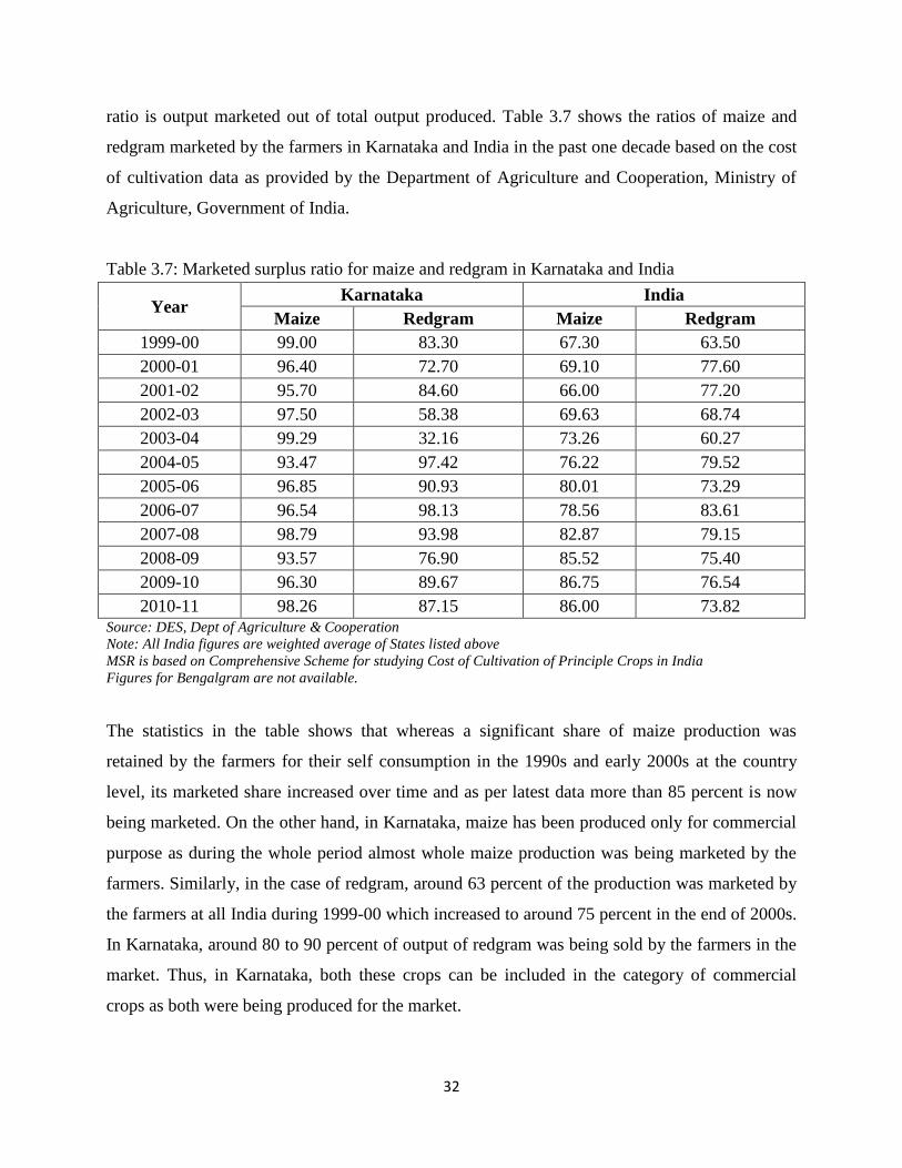
32
ratio is output marketed out of total output produced. Table 3.7 shows the ratios of maize and
redgram marketed by the farmers in Karnataka and India in the past one decade based on the cost
of cultivation data as provided by the Department of Agriculture and Cooperation, Ministry of
Agriculture, Government of India.
Table 3.7: Marketed surplus ratio for maize and redgram in Karnataka and India
Year Karnataka India
Maize Redgram Maize Redgram
1999-00 99.00 83.30 67.30 63.50
2000-01 96.40 72.70 69.10 77.60
2001-02 95.70 84.60 66.00 77.20
2002-03 97.50 58.38 69.63 68.74
2003-04 99.29 32.16 73.26 60.27
2004-05 93.47 97.42 76.22 79.52
2005-06 96.85 90.93 80.01 73.29
2006-07 96.54 98.13 78.56 83.61
2007-08 98.79 93.98 82.87 79.15
2008-09 93.57 76.90 85.52 75.40
2009-10 96.30 89.67 86.75 76.54
2010-11 98.26 87.15 86.00 73.82 Source: DES, Dept of Agriculture & Cooperation
Note: All India figures are weighted average of States listed above
MSR is based on Comprehensive Scheme for studying Cost of Cultivation of Principle Crops in India
Figures for Bengalgram are not available.
The statistics in the table shows that whereas a significant share of maize production was
retained by the farmers for their self consumption in the 1990s and early 2000s at the country
level, its marketed share increased over time and as per latest data more than 85 percent is now
being marketed. On the other hand, in Karnataka, maize has been produced only for commercial
purpose as during the whole period almost whole maize production was being marketed by the
farmers. Similarly, in the case of redgram, around 63 percent of the production was marketed by
the farmers at all India during 1999-00 which increased to around 75 percent in the end of 2000s.
In Karnataka, around 80 to 90 percent of output of redgram was being sold by the farmers in the
market. Thus, in Karnataka, both these crops can be included in the category of commercial
crops as both were being produced for the market.

33
Figure 3.1a: Marketed Surplus Ratio Maize and Red gram in Karnataka
Figure 3.1b: Marketed Surplus Ratio of Maize and Red gram in India
Figure 3.1a and 3.1b depict the marketed surplus ratio of maize and redgram in Karnataka and
India over the years. The dent showing low marketed surplus of redgram both in Karnataka and
India during 2003-04 may be due to the low rainfall received by the country and the state in the
years 2002-03 and 2003-04. As the crop depends only on rainfall, low rainfall in these two years
lowered the production and thereby farmers keeping higher share of the output for home
consumption during that year and may be keeping some amount for the coming year as well.
0.00
20.00
40.00
60.00
80.00
100.00
120.00
MS
R V
alu
es f
or
Ma
ize
an
d
Red
gra
m
Marketed Surplus Ratio: Karnataka
Karnataka Maize Karnataka Redgram
0.00 10.00 20.00 30.00 40.00 50.00 60.00 70.00 80.00 90.00
100.00
MS
R f
or
Maiz
e an
d R
edgra
m
Marketed Surplus Ratio: India
India Maize India Redgram

34
3.6 Trends in Consumption of Major Inputs
In the following paragraphs we discuss the trends in usage of high yielding variety (HYV) seeds,
irrigation, consumption of fertilizer, credit used by the farmers, the minimum support price
obtained for the selected crops and the estimates for farm mechanization. Table 3.8 below shows
the usage of HYV seeds of maize. Out of total area under maize , more than 90 percent was
found under using HYV seeds.
Table 3.8: Percentage of area under HYV for maize in Karnataka and India
Year Karnataka India
1993-94 94.49 50.31
1994-95 93.98 55.28
1995-96 93.13 59.83
1996-97 79.22 60.12
1997-98 96.54 47.41
1998-99 96.41 38.47
1999-00 95.48 29.59
2000-01 96.58 22.89
2001-02 96.71 22.82
2002-03 96.07 25.18
2003-04 95.62 22.52
2004-05 98.12 27.12
2005-06 98.18 29.03
2006-07 98.02 25.22
2007-08 97.75 35.11
2008-09 96.45 34.88
Source: Fertilizer Statistics of India, Indiastat.com
The area of maize under HYV in India has been decreasing over the years whereas the area
under HYV in Karnataka has been on the rise making its productivity an edge over India. The
higher percentage of area under HYV in the state shows the awareness of Karnataka farmers on
the advancement of technology taking place in maize.

35
Table 3.9: Percentage of irrigated area to cropped area for selected crops in Karnataka and India
Year Karnataka India
Bengal gram Maize Red gram Bengal gram Maize Red gram
1981-82 8 82 0 18 20 2
1982-83 8 79 0 16 22 2
1983-84 7 80 0 14 17 3
1984-85 6 74 0 15 18 4
1985-86 8 81 1 16 19 4
1986-87 8 80 2 19 21 4
1987-88 18 77 2 19 22 4
1988-89 14 76 2 17 21 4
1989-90 11 77 2 20 21 4
1990-91 12 74 2 13 20 4
1991-92 14 71 2 24 23 3
1992-93 10 65 2 22 22 3
1993-94 8 68 2 24 22 4
1994-95 6 66 3 21 22 4
1995-96 10 65 2 24 23 5
1996-97 10 54 2 26 21 6
1997-98 9 46 2 22 21 6
1998-99 11 53 1 21 10 4
1999-00 10 50 1 28 23 4
2000-01 11 48 1 31 22 4
2001-02 11 41 2 31 21 5
2002-03 11 39 2 32 20 5
2003-04 13 35 2 31 19 4
2004-05 17 38 2 31 21 4
2005-06 16 40 3 31 23 4
2006-07 15 38 4 31 22 4
2007-08 17 40 4 35 24 4
2008-09 17 40 5 33 25 5
2009-10 13 39 5 32 24 4 Source: DES, Ministry of Agriculture
Table 3.9 shows the percentage of area irrigated out of cropped area for selected crops in India
and Karnataka. It can be observed from the data that maize was produced mostly on the irrigated
land in Karnataka in the 1980s as more than 80 percent of area under maize was irrigated.
However, with the availability of HYV seeds and advancement of technology in maize whereby
ICRISAT has developed seed that can be more suitable for the dry land area, more and more
rainfed area has been brought under maize cultivation in the state. The percentage of irrigated
area under maize went down from around 80 percent in the 1980s to less than 40 percent in the

36
2000s in Karnataka. At the all India, maize irrigated area remains only in the range of 20 to 25
percent throughout the 1980s, 1990s and 2000s and thereby the crop at the all India is rainfed
crop. The other selected crops namely, bengalgram and redgram were cultivated with the help of
rainwater as very small area was irrigated for these crops both in the country as well as in the
state. Whereas in bengalgram, around 30 percent area was irrigated at all India, less than 20
percent was irrigated in Karnataka. Redgram on the other hand was mostly un-irrigated as less
than 10 percent area was irrigated both in the state and the country.
German scientist Justus Von Liebig invented the theory that Nitrogen (N), Phosphorous (P), and
Potassium (K) are the basis for determining healthy plant growth. The production of NPK
complex fertilizers commenced in 1960-61. Currently, India produces a large number of grades
of NP / NPK complex fertilizers. In addition, India produces various grades of simple and
granulated mixtures also of the same. In the year 2003-04, production of NPK/NPK complex
fertilizer was 4507 thousand tonnes.
Table 3.10 gives details about the consumption of NPK per hectares at the aggregate of all crops
by the farmers in Karnataka and India from 1981-82 to 2010-11. The use of NPK has been
increasing at the absolute level as well as per hectare in most of the states including Karnataka.
Comparing the state and all India, in the beginning of 1980s, consumption of NPK was almost
same in the country as well as the state. It was 34 kg per hectares in the state and the country in
1980-81. It increased to 70 kg in Karnataka and 67.6 kg in the country in 1990-91 and further to
164 kg in the state far above 146 kg in all India during 2010-11. Thus, the consumption of NPK
increased at a higher speed in Karnataka as compared to the country as a whole. The
consumption of fertilizer is basic for higher productivity. However, in the case of agriculturally
developed states like Punjab and Haryana where fertilizer consumption has gone beyond the
requirement and there is imbalance in the use of N, P, and K, the use of the same in Karnataka is
in the desired limits and it has not crossed the limit of desired amount.

37
Table 3.10: Consumption of NPK per hectare in Karnataka and India
(Kg/Hectare)
Year Karnataka India
1981-82 34.17 34.33
1982-83 34.40 37.06
1983-84 42.45 42.94
1984-85 50.65 46.57
1985-86 49.85 48.96
1986-87 47.86 49.54
1987-88 45.60 51.45
1988-89 67.67 60.57
1989-90 64.31 63.47
1990-91 70.83 67.55
1991-92 73.09 69.84
1992-93 62.86 65.45
1993-94 64.75 66.28
1994-95 68.49 72.13
1995-96 78.33 74.02
1996-97 66.95 73.92
1997-98 94.84 85.20
1998-99 93.31 87.65
1999-00 105.14 95.91
2000-01 109.77 90.66
2001-02 107.06 92.20
2002-03 95.36 91.66
2003-04 80.33 88.38
2004-05 100.98 96.05
2005-06 117.06 105.36
2006-07 119.46 112.53
2007-08 116.91 115.66
2008-09 148.11 127.51
2009-10 71.98 137.81
2010-11 163.94 146.32 Source: indiastat.com, DES, Ministry of Agriculture

38
Table 3.11: Minimum Support Price for the selected crops
( /Quintal)
Year Bengalgram Redgram Maize
1981-82 170 200 116
1982-83 235 215 118
1983-84 240 245 124
1984-85 250 275 130
1985-86 260 300 130
1986-87 280 320 132
1987-88 290 325 135
1988-89 325 360 145
1989-90 421 425 165
1990-91 450 480 180
1991-92 500 545 210
1992-93 600 640 265
1993-94 640 700 265
1994-95 670 760 290
1995-96 700 800 310
1996-97 740 840 320
1997-98 815 900 360
1998-99 895 960 390
1999-00 1015 1105 415
2000-01 1100 1200 445
2001-02 1200 1320 485
2002-03 1220 1320 490
2003-04 1400 1360 505
2004-05 1425 1390 525
2005-06 1435 1400 540
2006-07 1445 1410 540
2007-08 1600 1590 620
2008-09 1730 2000 840
2009-10 1760 2300 840
2010-11 1850 2950 880
2011-12 2100 3200 980 Source: Reserve Bank of India
Minimum Support Price (MSP) system was introduced in India after the inception of Agriculture
Price Commission (now Commission for Agricultural Costs and Prices) in the mid sixties. The
Commission declares MSP for 24 commodities including the cereals, pulses and oilseeds. There
is a support price for all the three selected crops. However, it should be noted that among the
selected crops, there is only declaration of MSP which is not supported by physical purchases.
However, still the MSP plays a big role in keeping the declared MSP of a particular crop as a

39
floor price for that crop, although farmers may get less than MSP in some cases. Over time,
support price has become a guaranteed income support rather than a price-risk hedge to the crop
growers. Table 3.11 presents MSP for bengalgram, redgram and maize over three decades. As
the Indian economy is growing thereby keeping the general prices and all other time series like
GDP, saving, investment, etc., increasing, there is a continuous increase in MSP of all the three
selected crops. The MSP of maize increased from 116 per quintal in 1981-82 to 980 per
quintal in 2011-12. Increase in MSP or pulse crops was much higher. MSP for bengalgram
increased from 170 per quintal in 1981-82 to 2100 in 2011-12 and redgram increased from
200 to 3200 during the same time period. There is increased demand for maize for the feed
purpose and price for pulse crops is increasing because of shortage of the same as compared to
demand for human consumption in the country. Therefore, higher MSP is offered by the
government for the selected crops in order to attract more farmers growing these crops by
expanding their area towards these crops as well as increasing input intensity like irrigation,
fertilizer etc., to increase their production level.
Paid out cost is the cost incurred by the farmers in growing a particular crop. It may not include
the imputed value of land as well as that of family labour. Table 3.12 depicts the paid out cost of
selected crops from 1999-00 to 2009-10 in Karnataka. The increase in the cost of cultivation can
be attributed to increase in quantity of inputs (like farm machineries, HYV seeds, equipments
used for irrigation, fertilizers etc) used and their high prices. The cost computed here excludes
the imputed value of family labour, owned value of inputs, rental value of owned land, interest
on fixed capital etc. The information on paid out cost also helps in the formulation of price
support policy and perhaps is the most significant one. The per hectare paid out cost was highest
in maize as compared to the pulse crops. The paid out cost for maize increased from 8
thousand per hectare in 1999-00 to 9 thousand per hectare in 2009-10 at constant 1999-00
prices. Similarly, cost of bengalgram increased from 4.6 thousand per hectare in 1999-00 to
7 thousand per hectare in a decade's period while redgram increased from 4 thouand to 4.9
thousand during the same time period. Thus, increase in paid out cost was higher in bengalgram
compared to maize as well as redgram.

40
Table 3.12: Paid out cost of selected crops in Karnataka (at 1999-00 Prices)
( /Hectare)
Year Bengal Gram Maize Redgram
1999-00 4620 8319 4030
2000-01 5068 8462 4588
2001-02 5808 7858 5138
2002-03 5511 8043 4984
2003-04 4483 7935 4089
2004-05 5975 10152 5699
2005-06 4803 8014 6326
2006-07 4621 8830 3974
2007-08 5832 9748 4742
2008-09 6691 10441 3764
2009-10 7147 9261 4893
Source: Farm Management Division, Govt. of Karnataka
Table 3.13: Agricultural credit (institutional) in Karnataka
Total agricultural Credit ( Lakh)
Agency/Category CBs SCB SCARDB RRBs Others Total
2008-09
Achievement 672463 290929 20438 228758 1852 1214440
Percent share in
total 55.37 23.96 1.68 18.84 0.15 100.00
Percent of Target
achieved 84.00 76.20 70.80 81.30 123.70 81.30
2009-10
Achievement 824081 307566 15064 320437 1505 1468653
Percent share in
total 56.11 20.94 1.03 21.82 0.10 100.00
Percent of Target
achieved 89.20 71.10 51.60 98.20 106.60 85.70
2010-11
Achievement 1773864 447272 19057 374852 0.00 2615045
Percent share in
total 67.83 17.10 0.73 14.33 0.00 100.00
Percent of Target
achieved 165.40 102.40 70.00 107.50 0.00 138.50
2011-12
Target 1375828 534492 28589 517699 2095 2458705
Percent share in
total 55.96 21.74 1.16 21.06 0.09 100.00
Source: State Focus Paper 2012-13
Note: Total Agricultural Credit = Crop Loan + Term Loan
CBs = Commercial Banks
SCBs = State Co-operative Banks
SCARDBs = State Co-operative Agriculture & Rural Development Banks
RRBs = Regional Rural Banks
Credit plays a huge role in spurring the private investment by the farmers which ultimately lead
to higher productivity in agriculture. During the decade of 2000s institutional credit has been

41
promoted by the Central as well as state government. The interest rate on institutional credit has
virtually been brought down to less than 5 percent and in certain cases it is only 2 to 3 percent for
agricultural purpose. Table 3.13 provides the information about the extension of credit by
various sources like commercial banks, state co-operative banks, regional rural banks etc. with
respect to agriculture. Agricultural credit has been calculated by adding crop loan and term Loan
by the same sources. The overall institutional credit increased from 12144 crore in 2008-09 to
24587 crore. The percentage of achievement of credit as compared to the target of various
sources was 81.3 percent in the year 2008-09 which increased to 85.7 percent in 2009-10 and
further it increased to 138.5 percent, exceeding the target. This was due to the financial literacy
in the state, which was emphasized for the benefit of villagers, along with opening of many
financial literacy and credit counseling centers for information dissemination. In all the three
years, share of commercial banks as the highest to get close to such high achievements.
In order to include maximum possible rural population into the banking fold, the government has
issued instructions to provide agricultural credit limit to all eligible farmers and issue Kisan
Credit Cards. Many Government of India schemes, like Dairy Entrepreneurship Development
Scheme, Poultry Development Scheme, etc., being implemented through NABARD, have
received enormous response from the public. This has paved way for better credit distribution
and improved opportunities for livelihood development. The credit flow to agriculture sector
during 2010-11 was 2615045 lakhs much higher than the previous year.
Table 3.14a and 3.14b provide the details of the distribution of amount borrowed by farmers
according to their size of land holding in Karnataka and India. This throws light on whether
various sources provide loan to farmers based on their income or size of land holding and which
source is opted by the farmers more-often? The farmers are divided into four category based on
the size of their land according to the standard definition. Table 3.15a shows the distribution of
100 among various sources providing loan to farmers in Karnataka. In the case of marginal
farmers 50 out of 100 was provided by money lenders followed by banks, co-operative society
and friends. Marginal farmers were stuck with the money lenders due to their ancestral debt
which gets carried on from generation to generation. For small farmers major source of credit
was banks followed by money lenders and co-operatives. For medium farmers, major source was

42
banks which provided nearly 50 of the total amount followed by co-operatives and money
lenders. Banks paid nearly 60 of the total amount in case of large farmers followed by co-
operatives and money lenders. The contributions from other sources was as low as nil. The state
figures also marked banks as the best source as they paid 50 out of the total amount of 100
followed by 20 which was paid by money lenders and 17 paid by co-operatives.
Table 3.14a: Per 100 distribution of outstanding loan taken by farmers in Karnataka
Karna
Taka
Govt. Co-operative
Society
Banks Agri/Professional
&
money lender
Trader Relatives&
Friends
Doctor ,
Lawyer etc.
Other All
Marginal
< 1 ha
2.6 10.1 24.3 50.1 1.4 8.9 0.4 2.3 100
Small
(1.01 to 2.0 ha)
1.4 22.3 35.0 30.2 1.4 8.2 0.0 1.6 100
Medium
(2.01-4.0 ha)
1.4 22.7 49.3 16.6 3.2 4.1 0.3 2.4 100
Large
(4.01+above ha)
2.2 18.5 59.6 12.5 1.7 3.6 0.7 1.5 100
Karnataka 1.9 16.9 50.1 20.0 1.9 6.8 0.4 2.1 100
Source: State Focus Paper 2012-13
Table 3.14b: Per 100 distribution of outstanding loan taken by farmers in India
All India Govt. Co-
operative
society
Ban
ks
Agri/Professional
& money lender
Trader Relatives
& Friends
Doctor,
Lawyer
etc.
Other All
Marginal
< 1 ha
3.2 12.3 24.1 36.6 4.5 15.7 1.0 2.6 100.0
Small
(1.01 to 2.0 ha)
1.7 20.5 35.4 25.9 4.2 8.8 0.8 2.6 99.9
Medium
(2.01-4.0 ha)
1.5 22.6 41.0 23.4 4.7 5.1 0.4 1.4 100.1
Large
(4.01+above ha)
1.4 22.8 42.8 20.1 5.4 5.4 1.0 1.3 100.0
Karnataka 2.5 19.6 35.6 25.7 5.2 8.5 0.9 2.1 100.1
Source: State Focus Paper 2012-13
Table 3.14b shows the distribution of 100 among various sources providing loan to farmers in
India. In case of marginal farmers 36 of the total amount was provided by money lenders
followed by banks ( 24), Co-operative society ( 12) and friends ( 16). For small farmers
major source of credit was banks contributing 35 to the total followed by money lenders ( 26)
and Co-operatives ( 20.5). For medium farmers, major source was banks which provided nearly

43
41 of the total amount followed by co-operatives and money lenders. Banks paid 43 of the
total amount in case of large farmers followed by co-operatives ( 23) and money lenders ( 20).
The contributions from other sources was as low as nil. The all India figures also marked banks
as the best source as they paid 36 of the total amount of 100 followed by 25 which was
paid by money lenders and 20 paid by co-operatives.
Table 3.15: Farm mechanization – physical and financial estimates for 2012-13 Lakh; Physical Hectares)
District
Tractors Power Tillers Farm Implements Miscellaneous Total
Physic
al
Bank
Loan
Physic
al
Bank
Loan Physical
Bank
Loan Physical
Bank
Loan Physical
Bank
Loan
Bagalkot 1036 3302 3030 2576 4027 3423 - - 8093 9300
Bangalore R 425 1434 723 813 1687 386 - - 2835 2634
Bangalore U 190 727 38 42 - - 135 103 363 872
Belgaum 1000 5525 300 306 - - 2200 655 3500 6486
Bellary 1220 5856 104 183 - - 50 440 1374 6479
Bidar 500 1875 150 113 - - 2000 765 2650 2753
Bijapur 1620 6998 400 540 1400 1260 - - 3420 8798
Chamrajnagar 210 905 40 46 - - - 700 250 1651
Chickballapur 200 842 200 238 300 127 5 95 705 1301
Chickmagalur 750 2340 400 480 1000 600 600 288 2750 3708
Chitradurga 1400 5950 505 601 650 497 - - 2555 7048
Dakshin Kannada 51 218 500 720 6600 5346 - - 7151 6284
Davangere 1965 10523 690 1149 2300 1974 - - 4955 13646
Dharwad 1000 4635 300 324 1920 1603 - - 3220 6562
Gadag 525 2244 230 290 - - 1000 270 1755 2804
Gulbarga 150 536 200 255 1002 354 - - 1352 1144
Hassan 160 680 720 1010 5100 2818 - - 5980 4508
Haveri 520 3042 44 71 1280 576 - - 1844 3689
Kodagu 350 1050 490 551 500 206 625 1406 1965 3214
Kolar 585 2340 625 750 500 200 - - 1710 3290
Koppal 500 2000 200 192 1400 896 - - 2100 3088
Mandya 225 928 250 469 1000 675 - - 1475 2072
Mysore 700 2940 350 364 501 654 160 128 1711 4086
Raichur 800 3000 400 390 50 450 500 563 1750 4403
Ramanagara 100 360 100 136 200 115 - - 400 611
Shimoga 400 1800 1000 1350 2 36 2400 4320 3802 7506
Tumkur 875 3290 390 496 1200 317 - - 2465 4103
Udupi 10 43 300 432 600 486 - - 910 961
Uttara Kannada 150 495 250 291 - - 880 704 1280 1490
Yadgir 180 643 60 77 244 109 - - 484 828
Karnataka 17797 76521 12989 15253 33463 23108 10555 10436 74804 125318 Source: State Focus Paper 2012-13
Farm mechanization facilitates timely completion of farm operations with desired degree of
precision. The benefits of farm mechanization includes preparation of a better seedbed, proper
placement of seeds, seedlings at the desired depth, better water management, better efficacy of

44
fertilizer / plant protection measures, timely harvest of produce and subsequent operations. These
in turn lead to minimizing the risks involved in farming, increasing the land productivity / crop
yield, increasing cropping intensity and above all, better farm returns. Drudgery in different
operations associated with conventional farming is reduced. Mechanization of post-harvest
operations help in value addition and is a good source of employment. The term “Farm
Mechanization” refers to a wide range of mechanized farming activities, and the activities or
investment being considered under the farm mechanization sector for credit planning purpose are
mainly that for crop production, viz., tractors, power tillers, combine harvesters and other
agricultural machinery, equipments and implements.
Table 3.15 provides the physical and financial estimates of farm mechanization for the year
2012-13. District wise information has been provided in the table. In order to interpret the
estimates for farm mechanization, the figures of the four districts (Belgaum, Bijapur, Davangere
and Gulbarga) along with that of the state is explained below. Among four districts selected as
study area for bengalgram, maize and regram; Davangere accounted to have spent maximum
amount for farm mechanization ( 13646) followed by Bijapur, Belgaum and Gulbarga. Both
physical and financial estimates of tractors were higher than any other farm machinery, in all
districts and in state, making it the most important machinery which is used for tilling,
ploughing, sowing and carrying the harvested produce from field to market. Though Belgaum
district did not report of using farm implements yet it was the machinery that was used maximum
after tractors. In most of the area, highest bank loans were also taken for tractors. Physical
estimates being lower and financial estimates being higher in the study area shows the better
facility of credit flow in and awareness of financial literacy among the farmers.
The gross cropped area in Karnataka during 2010-11 was 128.93 lakh hectare. It is assumed that
2.0 kw/hectare energy/power input is optimum for crop production system and farm
mechanization facilitates timely implementation of farm operations with desired degree of
precision. Tractors and power tillers have now become the prime source of motive power for
tillage, threshing and transport due to increase in cost of farm labour, especially for critical
operations like sowing and harvesting. With the growing popularity and adoption of custom-
hiring and scarcity of labour/draught animals, the holding size is fast losing relevance, as far as

45
estimating farm mechanization potential is concerned. However, it continues to influence the
ownership pattern and selection of equipments. The Input Surveys of Ministry of Agriculture,
Government of India revealed that the percentage growth of tractors, pump sets and threshers has
been higher in the marginal and small farm holding categories. Thus, the investment in farm
mechanization sector is now more demand driven.

46
Chapter IV
Marketed and Marketable Surplus of Major Foodgrains in Karnataka
An Empirical Analysis
After discussing in details about the agriculture in Karnataka vis-a-vis India in the previous
chapter, this chapter focuses on marketed and marketable surplus of selected crops, i.e.,
bengalgram, maize and redgram among the selected households. For this purpose a household
survey was carried out in the state among the farmers growing the selected crops. A sample size
of 422 farmers was surveyed in four districts of Karnataka, i.e., Belgaum, Bijapur, Davangere
and Gulbarga. The details of sample size and sampling methodology followed has already been
discussed in the Introduction Chapter. This chapter starts with the analysis of geographical
features of selected districts, the demographic profile of households selected, their cropping
pattern, output produced, inputs used, information dissemination, quantity sold, various channels
of marketing and losses incurred in various stages of production and marketing of the produce.
The analysis of primary survey has been done with respect to categorization of farmers into four
groups i.e. marginal, small, medium, large and aggregate of all groups. The households are
clubbed and analysis is done for the selected three crops as per the requirement of the study. Out
of 422 households surveyed, 89 were marginal farmers with operational holding between 0.00-
2.50 acres, 143 were small farmers with operational holding 2.51-5.00 acres, 84 were medium
farmers with operational holding 5.01-10.00 acres and the rest 106 were large farmers operating
above 10.00 acres of land.
4.1 Main Features of Agriculture in Selected Districts
4.1.1 Geographical Features of Selected Districts
The state of Karnataka in Southern India, lies between the 12.970
N latitude and 77.560
E
longitude and is bordered by the Arabian Sea and the Laccadive Sea to the West, Goa to the
North West, Maharashtra to the North, Andhra Pradesh to the East, Tamil Nadu to the South
East, and Kerala to the South West. The study is conducted on four districts, namely Belgaum,
Bijapur, Davangere and Gulbarga.

47
Table 4.1.1: Geographical area of selected districts
Geographical Area (sq. Km) 2011 Census
Sl.
No Districts Total
percent of
Dist Area to
Total Area
Location Co-ordinates
1 Belgaum 13,415 6.99 North-western part. Situated 2500 ft
above sea-level.
15.850 N latitude &
74.550E longitude
2 Bijapur 10.494 0.01 North-western part. 530 km northwest of
Bangalore.
16.830N latitude &
75.710E longitude
3 Davangere 5,924 3.09 Centre of the State. 14.46
0N latitude &
75.920E longitude
4 Gulbarga 16,224 8.46
Northern parts of the state. 200 km from
Hyderabad and 623 km north
of Bangalore
17.330N latitude &
76.830E longitude
Karnataka 191791 100.00 Sothern India
12.970 N latitude
and 77.560 E
longitude
Source: District at a Glance 2008-09
Table 4.1.2: Topography of selected districts
Topography of Districts
Sl. No Districts Zone Climate Topography
1 Belgaum
KA-8
Northern
Transitio
n Zone
Semi-
arid and
Arid
Predominantly a Kharif Zone, Shallow to medium black clay soil
and red sandy loam soil in equal proportion. The main crops
grown are - Rice, Jowar, Groundnut, Pulses, Sugarcane and
Tobacco
2 Bijapur
KA-3
Northern
Dry Zone
Semi-
arid and
Arid
A Rabi Zone. Soils are shallow to deep black clays in major
areas. The important crops grown are Rabi Jowar, Maize, Bajra,
Groundnut, Cotton, Wheat, Sugarcane and Tobacco.
3 Davengere
KA-4
Central
Dry Zone
Semi-
arid
A Kharif Zone. Soils are red sandy loam in major areas, shallow
to deep black in the remaining areas. The principle crops grown
are Ragi, Rice, Jowar, Pulses and Oilseeds.
4 Gulbarga
KA-2
North
East Dry
Zone
Semi-
arid
(wetter
half)
Predominantly a Rabi zone. The soils are deep to very deep black
clay in major areas and shallow to medium black in minor
pockets. The principle crops grown are Rabi Jowar, Bajra, Pulses,
Oilseeds and Cotton.
Source: http://www.uasbangalore.edu.in/asp/stations.asp
The total geographical area of the state is 191791 square km. Out of four selected districts,
Gulbarga was the largest district constituting the maximum of 8.5 percent area of the state
followed by Belgaum (7 percent), Davangere (3 percent) while Bijapur was the smallest selected
district occupying only 0.01 percent of the total area of the state (Table 4.1.1). District profile
shows that given the soil and climate of the district, the main crops grown in Belgaum districts
were rice, jowar, groundnut, pulses, sugarcane and tobacco. In Davengere, the principle crops

48
grown were ragi, rice, jowar some pulse and oilseed crops. The main crops in Bijapur, were
jowar, maize, bajra, groundnut, cotton, wheat, sugarcane and tobacco. Similarly, Gulbarga, had
jowar, bajra, pulses, oilseeds and cotton (Table 4.1.2).
4.1.2 Socio-economic indicators of the selected districts
The socio economic indicators of the selected districts are presented in Tables 4.1.3 to 4.1.5. It
can be observed from the statistics in Table 4.1.3 that although Belgaum had the highest
population but growth of population was the highest in Bijapur (20.38 percent). Davangere had
the lowest population among the four selected districts at the same time its population growth
rate was also lowest (8.71 percent). With the highest population, the density per square km was
also highest (356 per sq km) in Belgaum. Bijapur had the lowest density of 207 per sq km
against the lowest population district of Davenge. Literacy rate was found to be highest in
Davangere district i.e. 67 percent, with maximum number of males (76 percent) and females (58
percent) contributing towards the same. The gender ratio in the state as overall and in the study
area is almost the same ranging from 950-970 females per 1000 males.
Table 4.1.3: Demographic profile of selected districts
Population Census 2011
S. No. Districts Population Density
(per sq km)
Growth Rate of
Population (2001-
11)
Gender Ratio
(females per 1000
males)
1 Belgaum 47,78,439 356 13.38 969
2 Bijapur 21,75,102 207 20.38 954
3 Davangere 19,46,905 329 8.71 967
4 Gulbarga 25,64,892 233 17.94 962
Karnataka 6,11,30,704 319 15.67 968
Source:http://www.indiaonlinepages.com/population/karnataka-population.html
Among all the States in India, Karnataka holds the 7th
position in case of Human Development
Index and 6th
position in case of Gender Development Index; with a value of 0.650 and 0.637
respectively. Belgaum holds a better position among all selected districts, both in terms of HDI
and GDI, 8th
position and 9th
position, respectively.

49
Table 4.1.4 Literacy rate of selected districts
Literacy Rate Census 2001
S. No. Districts Male Female Total
1 Belgaum 75.7 52.3 64.2
2 Bijapur 68.1 46.19 57.46
3 Davangere 76 58 67
4 Gulbarga 61.8 37.9 50
Karnataka 76.29 57.45 67.04
Source: District at a Glance 2008-09Table 4.1.5: Human Development Index and Gender
Development Index for selected districts
Composition of HDI & GDI 2001
S. No. Districts HDI GDI
1 Belgaum 8 (0.648) 9 (0.635)
2 Bijapur 23 (0.589) 21 (0.573)
3 Davangere 12 (0.635) 13 (0.621)
4 Gulbarga 26 (0.564) 26 (0.543)
Karnataka 7 (0.650) 6 (0.637)
Source: HDR Karnataka 2005
Note: Figures in parentheses are HDI and GDI index values of the districts
4.1.3 Classification of Workers
Table 4.1.6 gives the details of classification of population into workers, non-workers, cultivators
and agricultural labourers according to 2001 Census. In Karnataka, out of total workers, 82
percent were main workers and only 18 percent were marginal workers. The same kind of ratio
was found in the study area of the state. Among the four districts, Belgaum had the maximum
towards non-workers, cultivators and agricultural labourers, whereas Davangere had the least in
the case of non-workers and agricultural labourers. The number of cultivators was lowest in
Bijapur.
4.1.4 Land Utilization in the Selected Districts
The pattern of land utilization reveals different usages of land in a particular area. Out of total
geographical area in the state, 55 percent was sown, 16 percent was covered with forest, 12
percent was the area not available for cultivation, uncultivated land excluding fallow land, which
included permanent pastures, trees and grooves and cultivable waste land was 9 percent and
fallow land was around 8 percent. Compared to the state average, all the selected districts had

50
higher area under cultivation. The percentage of area sown to total geographical area was above
80 percent in Gulbarga and Bijapur while it was between 60 to 70 percent in Belgaum and
Davengere.
Table 4.1.6: Classification of workers for selected districts
Classification Of Workers Census 2001 (numbers)
S.
No
Districts
Workers
Non-
workers
Cultivat
ors
Agricultural
Labourers
Total
Workers
(Main+
Marginal) Main Marginal
1 Belgaum 1537645
(81.89)
340129
(18.11) 2336731 706476 587476 1877774
2 Bijapur 551972
(76.85)
166241
(23.15) 1088705 217056 286699 718213
3 Davangere 631726
(80.60)
152054
(19.40) 1007171 219988 170138 783780
4 Gulbarga 1010434
(74.84)
339642
(25.16) 1780850 365267 539561 1350076
Karnataka
19364759
(82.28)
4170032
(17.72) 29315771 6883856 6226942 23534791
Source: District at a Glance 2008-09
Note: Figures in the parentheses are percentage to total workers, district-wise
Table 4.1.7a: Land utilization of selected districts (hectares) during 2010-11
Districts Belgaum Bijapur Davangere Gulbarga Karnataka
Geographical Area 1344382 1053471 597597 1094120 19049836
Forests 190424 1977 89918 35316 3071833
Area not
available for
cultivation
Non Agricultural Use 69663 36027 38992 38420 1430363
Barren 44342 29059 20533 35113 786627
Total 114005 65086 59525 73533 2216990
Other
Uncultivated
land*
Permanent pastures 24807 9575 19538 25855 912385
Trees and Grooves 3046 1316 4955 1131 285986
Cultivable waste land 11465 5502 8525 9417 414397
Total 39318 16393 33018 36403 1612768
Fallow land Current fallow 155784 86996 14036 22242 1199134
Other Fallow Land 6971 5685 5421 2624 426458
Total 162755 92681 19457 24866 1625592
Net area sown 837880 877334 395679 924002 10522653
Source: Directorate of Economics and Statistics, Ministry of Agriculture
Note: *Other Cultivated Land – excluding fallow land, Trees and Grooves are not included in Net Area
Table 4.1.7 b: Land utilization (in percent to total geographical area) of selected districts
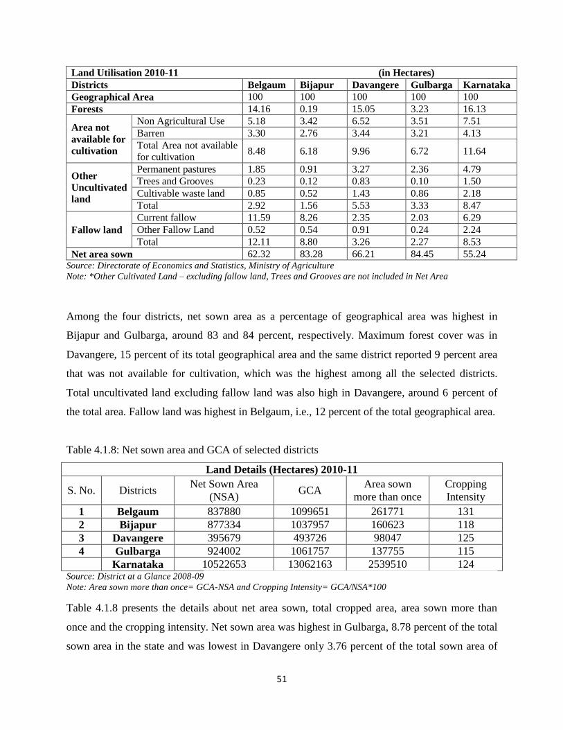
51
Land Utilisation 2010-11 (in Hectares)
Districts Belgaum Bijapur Davangere Gulbarga Karnataka
Geographical Area 100 100 100 100 100
Forests 14.16 0.19 15.05 3.23 16.13
Area not
available for
cultivation
Non Agricultural Use 5.18 3.42 6.52 3.51 7.51
Barren 3.30 2.76 3.44 3.21 4.13
Total Area not available
for cultivation 8.48 6.18 9.96 6.72 11.64
Other
Uncultivated
land
Permanent pastures 1.85 0.91 3.27 2.36 4.79
Trees and Grooves 0.23 0.12 0.83 0.10 1.50
Cultivable waste land 0.85 0.52 1.43 0.86 2.18
Total 2.92 1.56 5.53 3.33 8.47
Fallow land
Current fallow 11.59 8.26 2.35 2.03 6.29
Other Fallow Land 0.52 0.54 0.91 0.24 2.24
Total 12.11 8.80 3.26 2.27 8.53
Net area sown 62.32 83.28 66.21 84.45 55.24 Source: Directorate of Economics and Statistics, Ministry of Agriculture
Note: *Other Cultivated Land – excluding fallow land, Trees and Grooves are not included in Net Area
Among the four districts, net sown area as a percentage of geographical area was highest in
Bijapur and Gulbarga, around 83 and 84 percent, respectively. Maximum forest cover was in
Davangere, 15 percent of its total geographical area and the same district reported 9 percent area
that was not available for cultivation, which was the highest among all the selected districts.
Total uncultivated land excluding fallow land was also high in Davangere, around 6 percent of
the total area. Fallow land was highest in Belgaum, i.e., 12 percent of the total geographical area.
Table 4.1.8: Net sown area and GCA of selected districts
Land Details (Hectares) 2010-11
S. No. Districts Net Sown Area
(NSA) GCA
Area sown
more than once
Cropping
Intensity
1 Belgaum 837880 1099651 261771 131
2 Bijapur 877334 1037957 160623 118
3 Davangere 395679 493726 98047 125
4 Gulbarga 924002 1061757 137755 115
Karnataka 10522653 13062163 2539510 124
Source: District at a Glance 2008-09
Note: Area sown more than once= GCA-NSA and Cropping Intensity= GCA/NSA*100
Table 4.1.8 presents the details about net area sown, total cropped area, area sown more than
once and the cropping intensity. Net sown area was highest in Gulbarga, 8.78 percent of the total
sown area in the state and was lowest in Davangere only 3.76 percent of the total sown area of

52
the state. Among four districts, area sown more than once was highest in Belgaum (23.8 percent
of GCA in the district) and the cropping intensity of the district was also highest (131 percent).
Cropping intensity was the least (115 percent) in Gulbarga as area sown more than once being
the least. This may be due to the area being a dry region and irrigation facility was not optimum.
Irrigation is the major source of production for all the crops. In dry regions irrigation has a major
role to play. The districts selected for study area are all dry regions. As presented in Table 4.1.9,
in Belgaum, the major source of irrigation was tubewell providing irrigation to 29.61 percent of
the total irrigated area. Tanks contributed the least towards irrigation as only 0.14 percent of total
area was irrigated by the tank. In Bijapur, 33.97 percent of total area was irrigated by canals,
tanks contributing the least by providing irrigation to only 0.61 percent of total irrigated area.
Table 4.1.9a: Source-wise net irrigated area of selected districts
Net Irrigated Area 2010-11 (in Hectares)
S.No Districts Canals Tanks
Wells
Other
Source Total GCA
percent
of
Irrigated
Area to
GCA
Tube
wells
Other
wells
1 Belgaum 105019 696 143608 135008 100708 485039 1099651 44.11
2 Bijapur 106962 1908 91651 96515 17819 314855 1037957 30.33
3 Davangere 66203 1443 91203 786 12504 172139 493726 34.87
4 Gulbarga 34010 863 20800 28830 2610 87113 1061757 8.20
Karnataka 1156782 197047 1280523 437281 418171 3489804 13062163 26.72
Source: Directorate of Economics and Statistics, Govt. of Karnataka, 2010-11

53
Table 4.1.9b: Source-wise net irrigated area of selected districts (in percent)
Net Irrigated Area in percent 2010-11 (in Hectares)
S.No Districts Canals Tanks
Wells
Other Source Total GCA
percent
of
Irrigated
Area to
GCA
Tubewells Other wells
2 Belgaum 21.65 0.14 29.61 27.83 20.76 100 1099651 44.11
4 Bijapur 33.97 0.61 29.11 30.65 5.66 100 1037957 30.33
5 Davangere 38.46 0.84 52.98 0.46 7.26 100 493726 34.87
6 Gulbarga 39.04 0.99 23.88 33.09 3.00 100 1061757 8.20
Karnataka 33.15 5.65 36.69 12.53 11.98 100 13062163 26.72
In Davangere, major source of irrigation was tube well providing water facility to around 53
percent of total irrigated area. 39 percent of area in Gulbarga was irrigated by canals as a major
source of irrigation, followed by other wells, which irrigated 33 percent of total irrigated area. In
the state also tubewell was the major source of irrigation, irrigating 36.69 percent of total
irrigated area. The percentage of other wells and other sources of irrigation was quite high in
Belgaum, Bijapur and Gulbarga districts. This shows that the use of electrical tubewell for
irrigation is still lacking in the study area, which should be improved by creating awareness and
by facilitating farmers for the activity of borewell for tube as well as provision of cheaper
electricity.
Table 4.1.10: District-wise actual rainfall for selected districts in Karnataka
Actual Rainfall of Karnataka (mm) 2012
S.No District Jan Feb March April May June July Aug Sept Oct Nov Dec Total
1 Belgaum 2 1 7 30 76 117 206 124 114 108 34 6 825
2 Bijapur 2 3 6 18 44 89 87 86 167 100 24 7 633
3 Davangere 2 1 4 39 84 68 98 79 114 119 41 7 656
4 Gulbarga 3 4 8 19 38 122 159 168 200 97 20 5 843
Karnataka 2 3 8 37 91 189 272 199 160 134 45 11 1151
Source: Directorate of Economics and Statistics, Govt. of Karnataka, 2010-11
The data about rainfall depicts that from January to March, there was not much of rain in the
study area. Monsoon began in the month of April and became intense during the months of June
to October.

54
Graph 4.1: Actual rainfall distribution in selected districts of Karnataka
As can be seen from the graph, among all the four districts Gulbarga recorded the highest rainfall
of 843mm in 2012 and Bijapur recorded the lowest, 633mm during the same time period.
Maximum rainfall by individual districts was recorded in the month of July.
4.1.5 Cropping Pattern in Selected Districts
Cropping pattern in a particular area represents the area under various crops (food and non-food
crops). This gives an idea of crops sown in a particular area and the ratio of the same in an area.
In our analysis we have considered food crops that include total cereals, pulses, sugarcane and
fruits and vegetables; Similarly, non-food crops include oilseeds and fibers. According to this
definition of food and non food crops, Karnataka's share of food crops was much higher than that
of non-food crops constituting 78.40 percent and 21.60 percent, respectively. In the study area
the ratio of food crops and non-food crops according to this definition was 82:18, 86:15, 87:13,
and 92:8, respectively for Belgaum, Bijapur, Davangere and Gulbarga. Looking at the share of
foodgrains in total cropped area, Karnataka occupied around 68 percent area under foodgrains,
i.e., cereals and pulses. District wise, Belgaum, Bijapur, Davangere and Gulbarga occupied 52,
75, 81 and 89 percent of cropped area under foodgrains, respectively. Area under sugarcane and
fruits and vegetables was 5.3 percent and 5.4 percent, respectively in Karnataka. In the above
four districts, share of sugarcane in total cropped area was 27, 7, 2 and 2 percent, respectively
while share of fruits and vegetables was 3,4,4, and 1 percent, respectively.
0
200
400
600
800
1000
Rain
fall
(in
mm
)
Districts & Months
Rainfall Distribution
Belgaum
Bijapur
Davangere
Gulbarga

55
Table 4.1.11: District-wise area under principle crops in Karnataka during (2010-11)
Districts Belgaum Bijapur Davangere Gulbarga Karnataka
FOOD CROPS
Cereals
Rice 68469 71 142524 4542 1532261
Jowar 146160 190629 21771 212798 1242071
Bajra 19149 65452 1405 18875 309227
Maize 157511 75996 171511 7941 1260018
Ragi 1361 -- 15724 -- 750588
Wheat 54239 63974 733 17702 254755
Barley -- -- -- -- --
Other Cereals & Millets 1804 -- 578 20 23104
Total Cereals & Millets 448693 396122 354246 261878 5372024
Pulses
Gram 68213 156207 3917 208465 958704
Tur 5623 189677 6270 377775 889005
Other Pulses 34119 35740 6290 97854 926079
Total Pulses 107955 381624 16477 684094 2773788
Total food-grains 556648 777746 370723 945972 8145812
Sugarcane 282342 71343 10000 24471 644369
Total Fruits & Vegetables 34881 35840 16973 7736 656306
Total Food Crops 873871 884929 397696 978179 9446487
NON - FOOD
CROPS
Oilseeds
Groundnut 42950 68491 16797 5767 838026
Castor 374 2 254 68 18553
Sesamum 615 624 672 15782 85538
Rapeseed & Mustard 556 -- 16 15 3710
Linseed 2145 3209 -- 549 11358
Soybean 78662 -- -- 375 168033
Coconut 336 281 11377 238 440006
Nigerseed 491 1091 323 1034 23112
Sunflower 20869 59598 4689 32724 407950
Safflower Seeds 5901 5868 67 9877 55038
Others 364 321 253 -- 3532
Total Oilseeds 153263 139485 34448 66429 2054856
Fibres
Cotton 38331 10524 23061 13759 545288
Jute -- -- -- -- --
Mesta 4 -- -- 370 1907
Sunhemp -- -- -- -- 342
Others -- -- -- -- --
Total Fibres 38335 10524 23061 14129 547537
Total Non-Food Crops 191598 150009 57509 80558 2602393
Total Crops
Source: DES, Ministry of Agriculture, Govt. of Karnataka
The percentage of area under pulses in Karnataka out of total cropped area was 23. Among the
four selected districts namely, Belgaum, Bijapur, Davangere and Gulbarga the pulses share in
total cropped area was 10, 37, 4 and 65 percent, respectively. Thus Bijapur and Gulbarga had
higher intensity of pulse production compared to the other two districts. Unlike pulses, oilseeds
area was more uniformed across the districts, as they occupied around 17 percent of gross
cropped area in the state and around 14, 14, 8 and 6 percent area in Belgaum, Bijapur, Davengere

56
and Gulbarga districts, respectively. Total fibers occupied around 5 percent of gross cropped area
in Karnataka while its share in the selected districts varied from 1 to 5 percent of gross cropped
area.
So, it can be said that most of the area in the selected districts was under cereals, pulses and
oilseeds and fruits & vegetables had the least area allocated in the selected districts. Therefore,
the production of cereals and pulses was higher in the selected districts along with oilseeds as
compared to fruits and vegetables and fiber crops.
4.1.6 Macro Overview of Selected Districts
Tables 4.1.12 and 4.1.13 presents the macro picture of agriculture and allied Sector in the study
area and their respective contribution towards Gross District Domestic Product (GDDP) and
Gross State Domestic Product (GSDP).
Table 4.1.12: Share of agriculture and allied sector in GDDP
Gross District Domestic Product for Karnataka during 2008-09 at Constant (2004-05 prices)
Sl No District
Agriculture
including
animal
husbandry
Forestry
&
Logging
Fishing
Total
Agri. &
Allied
Sector
GDDP
Per
capita
GDDP
(in
Rs.)
District-
wise Share
of Agri &
Allied
Sector in
GDDP
( percent)
1 Belgaum 289043 29714 988 319745 1333267 28863 23.98
2 Bijapur 122574 11985 1158 135717 470447 23754 28.85
3 Davangere 131957 13116 2373 147446 593319 30225 24.85
4 Gulbarga 168724 19125 904 188753 776291 22622 24.31
Karnataka 3254486 464366 86811 3805663 5637262 223294 15.66
Source: Economic Survey of Karnataka 2012-13
Agriculture and allied sector has been divided into three categories: agriculture including animal
husbandry, forestry & logging and fishing. Category-wise contribution of the above mentioned
three categories towards total GSDP of agriculture and allied sector was 85.51 percent, 12.20
percent and 2.28 percent, respectively in the state as a whole. Contribution of the agriculture and
allied sectors in the districts of the study area for the aggregate district GDDP was nearly 25

57
percent, with state agriculture making a contribution of 15.66 percent to the total state domestic
product. It is revealed from the table that agriculture played much more role in the district
income compared to the role of agriculture in the GSDP of the state. Shift towards services
sector dominance has been attributed mainly to high marginal propensity to consume and
technological advancements in areas such as software development, trade, and communications.
Table 4.1.13: GDDP, NDDP, PCI and GSDP
Gross / Net District Domestic Product and Per Capita Net District Income for the year 2010-11
(Provisional) ( Crore)
Sl.No District
At Current Prices At 2004-05 prices Per captia
Income (Net
District Domestic
Product (NDDP)
at Current
Prices) (in )
Share of each
district in total
GSDP at 2004-05
prices during
2010-11
GDDP NDDP GDDP NDDP
1 Belgaum 22297 19876 15476 13643 42125 5.7
2 Bijapur 8828 8053 5620 5073 39809 2.07
3 Davangere 9467 8562 6421 5757 42701 2.37
4 Gulbarga 10113 9104 6416 5697 37394 2.36
Karnataka 406470 361371 271485 238647 61073 100
Source: Economic Survey of Karnataka 2012-13
Table 4.1.13 presents the details of GDDP and NDDP at current and at 2004-05 prices (recent
base year). Per capita income of the state at current year prices was 61073 and that of the
country was estimated at 53331 in the year 2010-11 (released by Central Statistical
Organisation). Compared to the state average, per capita income was 42701 in Davangere,
42125 in Belgaum, 39809 in Belgaum and 37394 in Gulbarga. Thus all the four selected
districts had much less per capita income compared to the state as well as the country average.
Belgaum was found to be having a maximum share in the total GSDP of the state, 5.7 percent
while all other districts constituted only around 2 percent to total GSDP.
4.2 Main Features of Sample Households
4.2.1 Socio-economic Profile
As mentioned in the methodology, the survey was conducted taking 422 households into
consideration of which 89 farmers fell in the category of marginal farmers, 143 under small
farmers, 84 under medium farmers and 106 under large farmers; growing bengalgram, maize,
and redgram as their main crop as shown in Table 4.1 below. Among the selected households

58
marginal farmers constituted 21 percent, small farmers 34 percent, medium farmers 20 percent
and large farmers had a ratio of 25 percent of the total selected households.
Table 4.2.1: Details of selected households
Households Farm size wise
FMC Marginal Small Medium Large All Farms
Households 89
(21.1)
143
(33.9)
84
(19.9)
106
(25.1)
422
(100.0)
The District wise details have been depicted in Table 4.2.2. It is seen from the table that 70
farmers were selected from Belgaum, 140 from Bijapur, 70 from Davangere and 142 from
Gulbarga. Farm size wise, 27 marginal farmers, 25 small farmers, 14 medium farmers and only 4
large farmers were selected from the Belgaum district. In Bijapur district, there were 20 marginal
farmers, 44 small farmers, 36 medium farmers and 40 large farmers selected. From Davangere
district, 14 marginal farmers, 26 small farmers, 19 medium farmers and 11 large farmers were
selected. In Gulbarga district, the selection was of 28 marginal farmers, 48 small farmers, 15
medium farmers and 51 large farmers. As mentioned above in this way a total number of 422
households were selected from the above mentioned four districts.
Table 4.2.2: Households details district-wise
FMC Belgaum Bijapur Davangere Gulbarga Total
Marginal 27 (38.6) 20 (14.3) 14 (20.0) 28 (19.7) 89 (21.1)
Small 25 (35.7) 44 (31.4) 26 (37.1) 48 (33.8) 143 (33.9)
Medium 14 (20.0) 36 (25.7) 19 (27.1) 15 (10.6) 84 (19.9)
Large 4 (5.7) 40 (28.6) 11 (15.7) 51 (35.9) 106 (25.1)
All Farms 70 (100.0) 140 (100.0) 70 (100.0) 142 (100.0) 422 (100.0) Note: Figures in parentheses are respective percentages of total
The Socio-economic Profile of the sampled households is presented in Table 4.2.3. The main
occupation of all the households was agriculture. There were a number of farmers, who had
reported sub occupation too. Out of total marginal farmers, 3.37 percent had dairy as their sub
occupation, 3.37 percent had gone for services, 12.36 percent were farm labourers, and 8.99
percent opted for other sub occupations. Out of total small farmers, 3.50 percent had dairy as
their sub occupation, 4.90 percent went for services, 10.49 percent were farm labourers, and 5.59

59
percent opted for others. Among the medium farmers, 4.76 percent opted for dairy, 3.57 percent
went for services, 10.71 percent were farm labourers and 4.76 percent went for others. None of
the large farmers opted for dairy as their sub occupation while services, farm labour and other
occupations occupied 4.72 percent, each in the total sub occupation. Among the above
mentioned sub occupations, farm labour had the major share among marginal, small and medium
farmers and was the least in the case of large farmers.
Table: 4.2.3: Characteristics of sampled population
Characteristics Marginal Small Medium Large Total
Age of decision maker (yrs) 45.61 45.89 48.58 46.08 46.41
Main Occupation ( percent) 100 100 100 100 100
Sub Occupation ( percent)
Dairy 3.37 3.50 4.76 0.00 2.84
Service 3.37 4.90 3.57 4.72 4.27
Farm labour 12.36 10.49 10.71 4.72 9.48
Others 8.99 5.59 4.76 4.72 5.92
Education(Avg. years of schooling) 5.22 4.72 5.15 7.08 5.50
Family Size (No in Average) 5.87 6.45 6.46 8.62 6.87
Male 2.27 2.52 2.57 3.29 2.67
Female 1.89 2.17 2.20 2.75 2.27
Children 1.71 1.75 1.67 2.58 1.93
Social Grouping (No of Households)
General 31 64 46 66 207
SC/ST 19 28 11 9 67
OBC 39 51 27 31 148
Others
Gender of head of household (percent)
Male 96.63 97.20 97.62 99.06 97.63
Female 3.37 2.80 2.38 0.94 2.37
Note: family size including permanent labour
The head of the households was male dominated (97.63 percent) with very few households
having a female head (2.37 percent). The average age of the decision maker of the family in all
sampled households was 46.41 years. Based on the farm-size category, average age of marginal,
small, medium and large farmers was 45.61, 45.89, 48.58, and 46.08 years, respectively. The
average years of schooling of the sample farmers were 5.50 years with highest (7.08 years) in
case of large farmers and lowest (4.72 years) in the case of small farmers. The 5.5 years of
average schooling indicates that on an average the selected households had their education up the
primary level. There was no significant difference in educational standards across farm size. The

60
average family size of all the households in the study area was 6.87 of which 2.67 were males
and 2.27 were females and 1.93 were children. The largest average family size was of large
farmers (8.62) and the smallest family size was of marginal farmers (5.87), showing a direct
relationship between farm size and family size. In the case of social grouping, most of the
farmers belonged to General category followed by Other Backward Castes (OBCs) and
Scheduled Caste/Scheduled Tribe (SC/STs). Overall, 49.05 percent of sample farmers belonged
to General category, 35.07 percent to OBCs and 15.88 percent belonged to SC/ST category.
Looking at the farm-size, 43.82 percent of marginal farmers were OBC followed by 34.83
percent General and 21.35 percent SC/ST. Within the small farmers, 44.76 percent were General
followed by 35.66 percent OBC and 19.58 percent SC/ST. In the case of medium farmers, 54.76
percent were General followed by 32.14 percent OBC and 13.10 percent SC/ST. Among large
farmers, 66 percent belonged to General, 31 percent OBC and 9 percent SC/ST.
4.2.2 Land Ownership Pattern/ Operational Holding Characteristics
The characteristics of operational holding and land ownership pattern of the sample households
is depicted in Tables 4.2.4 to 4.2.6. The average household operated area among the selected
households was 3.76 hectares. the average size of marginal holdings was 0.718 hectares followed
by 1.561 hectares of small farmers, 3.108 hectares of medium farmers and 9.808 hectares of
large farmers. An increasing pattern can be observed in the case of eased-in and leased-out land
with the farm size indicating large farmers having higher tendency of tenancy compared to small
farmers. However, whole of irrigated area was cultivated as irrigated land was neither leased-out
nor it in the category of waste land or non cultivable land in any farm size category. Out of total
operated area, the irrigated area was only miniscule, only 16 percent of total operated area while
84 percent operated area was unirrigated. Only unirrigated area was available for tenancy.
Average irrigated operated area was 0.617 hectares and average unirrigated operated area was
3.145 hectares. While all the categories had leased-in some of the operational area, only medium
and large category farmers were found to lease-out some part of their land.

61
Table 4.2.4: Operational holding characteristics (per hectare)
Size
Class of
Farm
Owned
Land
Leased-in
Land
Leased -
out land
Wasteland Non-
Cultivable
Land
Net
Operational
Holding
Net
Opera
ted
Area
Type of
Land
Irr Unirr Irr Unirr Irr Unirr Irr Unirr Irr Unirr Irr Unirr Irr+Un
irr
Marginal 0.15 0.56 0.005 0.009 0 0.000 0 0.005 0 0.005 0.154 0.563 0.718
Small 0.31 1.22 0.011 0.021 0 0.000 0 0.003 0 0.000 0.319 1.242 1.561
Medium 0.67 2.22 0.164 0.104 0 0.039 0 0.000 0 0.014 0.834 2.274 3.108
Large 1.24 7.46 0.000 1.253 0 0.103 0 0.004 0 0.031 1.237 8.571 9.808
Total 0.58 2.85 0.037 0.344 0 0.034 0 0.003 0 0.012 0.617 3.145 3.762
Note: The values reported are average values
Table 4.2.5: Source of irrigation
Size Class of
Farm
Source of Irrigation ( percent)
Surface/
Canal
Tube Well/
Ground-Water Borewell Tanks Others Total
Marginal 73.47 8.84 14.74 2.95 0 100.00
Small 57.33 23.11 10.67 8.89 0 100.00
Medium 78.90 17.05 0.00 4.05 0 100.00
Large 67.90 22.53 0.00 9.57 0 100.00
Total 69.31 20.44 2.64 7.62 0 100.00 Note: Source = percent of Total Irrigated Area Farm size wise
Table 4.2.5 shows the percentage share of different sources of irrigation by different farm size
groups. The various channels of irrigation opted by farmers were canal, tubewell, borewell, and
tanks. Maximum area was irrigated by using canal by all the farm size groups. In the case of
marginal farmers, 73.47 percent of the area was irrigated by canal, 14.74 percent by borewell,
8.84 percent by tubewell and 2.95 percent by tanks. In the case of small farmers, 57.33 percent of
the area was irrigated by canal, 23.11 percent by tubewell, 10.67 percent by borewell and 8.89
percent by tanks. For medium farmers, 78.90 percent area was under canal irrigation, 17.05
percent was irrigated by tubewell and 4.05 percent was irrigated by tanks. In the case of large
farmers, 67.90 percent was irrigated by using canal, 22.53 percent by using tubewell and 9.57
percent by using tanks. Borewell was not used by medium and large farmers.
Out of total operated area of 3921.73 acres, only 398 acres was leased-in. The majority of area
(12.8 percent) was leased-in by large farmers while marginal farmers leased-in only 1.9 percent

62
of total operated area. Small farmers leased-in 2.1 percent and medium farmers leased-in 8.6
percent of their total operated area. Out of total operated area around 10 percent was under
tenancy. The percentage of farmers who leased in was not much different from the area leased-in
as around 10.7 percent of all farmers leased-in some land. Across various categories, 3 and 5
percent of marginal and small farmers respectively, and 14 and 22 percent of medium and large
farmers, respectively leased-in some land. Irrespective of the category, all sample farmers
leased-in on fixed amount of money and there was no leasing-in on produce sharing basis. The
average rent for leasing-in per hectare was 12538 that varied from 17221 in the case of
medium farmers to 11655 in the case of large farmers. Overall 10.66 percent of total
households leased-in 10.15 percent of total operated area for 12538 per hectare.
Table 4.2.6: Terms of leasing
Size
Class of
Farm
Incidence Terms ( percent) Rent
percen
t Area
leased
-in
percen
t HHs
leasin
g -in
For
fixed
money
Fixed
produce
Share of
Produce
Others For fixed
money
Fixed
produce
Share of
Produce
percent
(Qtl.) (
percent)
(Rs./Ha) (Qtl.) (
percent)
Marginal 1.90 3.37 100 0 0 0 16055.00 0 0
Small 2.09 4.90 100 0 0 0 14229.35 0 0
Medium 8.61 14.29 100 0 0 0 17221.02 0 0
Large 12.77 21.70 100 0 0 0 11654.56 0 0
Total 10.15 10.66 100 0 0 0 12538.35 0 0
Note: percent is calculated for area leased-in out of total operated area, Farm size wise
4.2.3 Cropping Pattern and Physical Crop Productivity
The cropping pattern in a particular area depends on many factors like amount of rainfall,
irrigation, soil and climate of a particular place and also the economic attitude of the farmers.
Tables 4.2.7a and 4.27b depict the cropping pattern followed by the selected farmers. All the
crops grown by the selected farmers have been grouped into kharif, rabi and perennial crops.
The first table presents area under a particular crop in hectares while second table gives the
details in its percentage in gross cropped area. At the aggregate, kharif crops constituted the
highest share in the gross cropped area of the selected households. Kharif crops constituted 64
percent share of all cropped area, rabi crops had a share of 33 percent while perennial crops
contributed only 3 percent in the gross cropped area. Across various farm size categories, the

63
share was almost same ranging between 60 to 65 percent for kharif crops, 31 to 38 percent for
rabi crops and 1 to 3 percent for the perennial crops.
Table 4.2.7a: Cropping pattern - area (hectares)
Farm Size Marginal Small Medium Large Total
Kharif Season
Redgram 28.057 101.032 124.919 654.657 908.664
Maize 25.931 66.194 81.376 124.899 298.400
Jowar 3.239 4.352 7.288 63.158 78.037
Cotton 5.668 9.109 51.012 65.789
Other Oilseeds 1.012 2.642 1.619 10.122 15.395
Vegetables 0.405 0.810 1.619 2.834
Groundnuts 0.405 2.024 11.336 13.765
Onion 5.162 3.441 9.312 17.915
Greengram 0.810 5.344 10.121 16.275
Other Coarse Cereals 0.506 1.822 2.024 7.692 12.045
Total Kharif 59.960 193.431 233.420 942.308 1429.119
Rabi Season
Bengalgram 19.787 64.787 46.741 243.725 375.040
Maize 15.587 38.209 30.567 72.065 156.427
Jowar 1.619 13.036 20.243 120.567 155.466
Wheat 2.024 4.858 19.717 26.599
Other Oilseeds 0.810 8.097 8.907
Vegetables 1.012 1.012 8.097 6.478 16.599
Any Others 0.202 0.202
Total Rabi 38.006 119.271 111.316 470.648 739.241
Perennial
Sugarcane 0.911 10.526 8.097 32.794 52.328
Vegetables 0.810 0.810
Any Others 0.405 3.036 7.692 11.134
Total Perennial 0.911 10.931 11.943 40.486 64.272
Note: Any Others include Arecanut, Banana, Chilli, Palm, Grass, and Flower
Other Oilseeds include Saffola seeds and Sunflower
Other Coarse Cereals include Pearl Millet and Ragi

64
Table 4.2.7b: Cropping pattern - Percentage of gross cropped area
Farm Size Marginal Small Medium Large Total
Kharif Season
Redgram 28.375 31.218 35.023 45.042 40.699
Maize 26.226 20.453 22.815 8.593 13.365
Jowar 3.276 1.345 2.043 4.345 3.495
Cotton 1.751 2.554 3.510 2.947
Other Oilseeds 1.024 0.816 0.454 0.696 0.690
Vegetables 0.409 0.250 0.454 0.127
Groundnuts 0.125 0.568 0.780 0.617
Onion 1.595 0.965 0.641 0.802
Greengram 0.819 1.651 0.000 0.696 0.729
Other Coarse Cereals 0.512 0.563 0.568 0.529 0.539
Total Kharif 60.641 59.769 65.443 64.833 64.011
Rabi Season
Bengalgram 20.012 20.019 13.104 16.769 16.798
Maize 15.764 11.806 8.570 4.958 7.006
Jowar 1.638 4.028 5.675 8.295 6.963
Wheat 0.625 1.362 1.357 1.191
Other Oilseeds 0.227 0.557 0.399
Vegetables 1.024 0.313 2.270 0.446 0.743
Any Others 0.063 0.009
Total Rabi 38.438 36.854 31.209 32.382 33.111
Perennial
Sugarcane 0.921 3.253 2.270 2.256 2.344
Vegetables 0.227 0.036
Any Others 0.125 0.851 0.529 0.499
Total Perennial 0.921 3.378 3.348 2.786 2.879
Grand Total 100.00 100.00 100.00 100.00 100.00
Note: Any Others include Arecanut, Banana, Chilli, Palm, Grass, and Flower
Other Oilseeds include Saffola seeds and Sunflower
Other Coarse Cereals include Pearl Millet and Ragi
Among the kharif crops, redgram and maize constituted the highest area at the aggregate. The
percentage of redgram and maize in the gross cropped area at the aggregate was 41 and 13
percent, respectively. The other main kharif crops were jowar and cotton constituting around 3
percent each of the gross cropped area. Vegetables, groundnut and greengram were the other
minor kharif crops among the selected households. Across various farm size categories also
redgram and maize occupied the highest share in the kharif crops. Looking at the rabi crops,
bengalgram, maize (rabi) and jowar were the principal crops that occupied the major share.
Benalgram occupied 17 percent share of the gross cropped area while rabi maize and rabgi jowar
occupied around 7 percent share each in the gross cropped area. Wheat, vegetables and other

65
oilseeds were the other minor rabi crops with combined area of less than 2 percent in the gross
cropped area. Across farm size categories, bengalgram, maize and jowar were the main rabi
crops among marginal, small and medium farmers, the large farmers had bengalgram, jowar and
maize as major rabi crops in that order. Sugarcane was the main perennial crop occupying less
than 1 percent of gross cropped area among the marginal farmers, and 2 to 3 percent among all
other category of farmers. Thus, at the aggregate, the major concentration of cropping pattern
among the selected households was on redgram, bengalgram, kharif and rabi maize and kharif
and rabi jowar.
Table 4.2.8: Crop wise yield observed by the selected farmers (kg/hectare)
Marginal Small Medium Large Total
Kharif Season
Redgram 746.42 700.80 744.77 882.36 839.06
Maize 3940.98 3844.00 3977.95 3372.73 3691.70
Jowar 1327.61 781.20 1166.38 1070.33 1073.86
Cotton 398.72 408.37 405.98 405.69
Other Oilseeds 395.22 529.96 494.01 494.00 493.68
Vegetables 3705.53 1235.03 4631.34 3528.71
Groundnuts 740.92 123.50 843.61 734.69
Onion 3932.66 3312.70 3823.11 3756.63
Greengram 988.02 383.59 186.73 291.24
Other Coarse Cereals 1086.74 1097.76 839.80 559.00 709.86
Rabi Season
Maize 3396.97 3373.59 3122.69 2599.12 2970.10
Bengalgram 845.95 793.55 957.71 917.27 897.17
Jowar 988.02 1058.58 879.31 865.08 884.44
Wheat 0.00 988.00 1070.33 633.98 740.62
Other Oilseeds 753.36 684.87
Vegetables 4248.59 2074.69 2618.19 447.70 1837.45
Any Others 988.14 988.14
Perennial
Sugarcane 74651.44 72256.42 84794.74 62603.68 68188.98
Vegetables 0.00 0.00 4322.59 0.00 4322.59
Any Others 0.00 4939.49 5598.74 5043.94 5191.45
Note: Any Others include Arecanut, Banana, Chilli, Palm, Grass, and Flower
Other Oilseeds include Saffola seeds and Sunflower
Other Coarse Cereals include Pearl Millet and Ragi
In Bijapur and Gulbarga, most of the surveyed farmers cultivated redgram and bengalgram,
whereas maize was cultivated by the farmers of Davangere and Belgaum. Therefore total area
under redgram accounted for the highest share of about 40.7 percent. The next predominant crop

66
was maize in both the seasons (20.4 percent) followed by bengalgram (16.8 percent). Rest 22
percent of area was accounted by other food and non-food crops like jowar, cotton, oilseeds,
wheat, groundnuts, sugarcane, etc.
Table 4.2.8 presents the crop productivity observed by the selected households. The average
yield of redgram was 8 quintals per hectare that varied between 7 to 8 quintals among different
farm size categories. Maize productivity varied between 34 and 40 quintal per hectare while
average yield of maize was observed as 37 quintals per hectare in the kharif season. Against the
kharif season, the productivity of maize in rabi season was far less only 30 quintals per hectare
and it varied bween 26 and 34 quintals per hectare. The jowar productivity was 11 quintals per
hectare in kharif season and 9 quintal per hectare in rabi season. The variation in productivity of
jowar across various farm size holdings was far higher in the kharif season as compared to the
rabi season. Cotton productivity was 4 quintal per hectare and hardly there was any variation
across the farm size holdings. Productivity of sugarcane varied between 626 and 848 quintals per
hectare while average productivity was 682 quintal per hectare among the selected households.
4.2.4 Investment Pattern
The usage and ownership of farm machineries and implements by different farmers signifies
their degree of mechanization in agriculture. It not only brings out technological dualism
prevailing in the area among the group of farmers but also points reasons for different levels of
productivity in the area due to different degree of technology adoption. The detail of average
investment per hectare by the selected farmers is provided in Table 4.2.9 and the investment
pattern in livestock in Table 4.2.10. The different mechanical assets owned by the farmers were
reported in terms of their present value. The ownership of tractor was non-existent among the
marginal farmers while in all other categories tractor ownership was reported by some farmers.
The table presents average value of assets owned by the farmers per hectare. As can be observed
from the table, none of the sample households under study opted for combined harvester.
Average value of tractor was the highest followed by tubewell and threshing machine. The value
of ownership of tractor varied between 11664 for the small farmers, 9309 for the medium
farmers and 7573 for the large farmers while its value at the aggregate was 8129.

67
Table 4.2.9: Ownership of farm machinery by the selected households
Size of Farm
Class
Level of Investment in per Hectare
Tractors Combined
Harvester
Threshing
Machine
Tube
Well
Total
Marginal 0 0 0 8226.26 8226.26
Small 11664.42 0 0 6191.12 17855.54
Medium 9309.27 0 76.62 7845.84 17231.74
Large 7573.86 0 240.44 2077.40 9891.71
Total 8129.08 0 170.08 3850.68 12149.84
Note: Average Investment per Hectare
Marginal and small farmers did not report of any investment with respect to threshing machine,
whereas large farmers invested around 240 hectare in threshing machine. Per hectare
investment in irrigation tubewell varied between 2077 and 8226 by different farm size
holdings. The aggregate investment per hectare was 8 thousand by the marginal farmers, 18
thousand by the small and medium farmers and 10 thousand by the large farmers.
Table: 4.2.10. Livestock ownership by selected farmers
Size of Farm Cattle Buffalo Others Total
Marginal 14140.45 6966.29 1224.72 22331.46
Small 17702.80 7573.43 2006.99 27283.22
Medium 20351.19 12892.86 3154.76 36398.81
Large 29948.11 11188.68 19721.70 60858.49
Total 20554.50 9412.32 6520.14 36486.97 Note: Level of Investment Rs. / HHs, Others mainly include- Oxen
The distribution of livestock by farm size groups is provided in Table 4.2.10. The level of
investment is calculated in per household by farm size. As the value of livestock ownership is
measured in terms of per household, it has direct relationship with farm size. The bigger size
holding farmers rear more numbers of livestock. Per household livestock value increased from
22 thousand for marginal farmers to 27 thousand for small farmers, 36 thousand for medium
farmers and 61 thousand for the large farmers. The level of investment was highest for cattle
( 20.5 thousand) followed by buffalo ( 9 thousand) and others ( 6.5 thousand).

68
4.3 Estimation of Crop Losses at Different Stages
Between the crop sowing and harvesting, there are various stages of growth of the plants. After
the maturity, the crop is harvested, threshed and winnowed and the total grain thus is available
for final consumption or for intermediate processing. The produce obtained after harvest,
threshing and winnowing, still has to go through different phases until it reaches the market and
the final consumer. Generally, farmers retain certain amount of the food grain or other food and
non food crops for their own consumption, seed, feed and payment in kind. Yet some amount
may be stored to be sold later for obtaining better price in the off season. In all theses processes
farmers have to bear with some crop loss at different stages. Some amount is lost during the
growth period of the crop known as pre-harvest losses in terms of pests and diseases. Certain
amount of loss occurs in the harvesting process in both manual harvest as well as mechanical
harvest. Yet another category of losses occur known as post harvest losses. The latter are
categorized as threshing, winnowing, transportation and storage losses. As the present analysis
pertains to marketing of the produce, we ignore the first category of losses, i.e., pre harvest
losses and shall concentrate only on harvesting and post harvesting losses.
4.3.1 Crop Loss on Farm (Harvesting, Threshing and Winnowing)
Harvesting and post harvest losses occurs because of several reasons. Some of these losses are
natural losses and cannot be avoided whereas some others are due to poor apparatus and they can
be minimized. For example, the losses that occur due to poor methods of harvesting,
transportation and storage can be minimized by adopting appropriate methods either manual or
mechanical. Tables below provide the details of crop loss on farm due to harvesting, threshing
and winnowing of the three major crops under study, namely bengalgram, maize and redgram.
The losses are calculated over total production for each crop individually by farm size categories.
The details of mode of techniques (manual and mechanical) used for performing the above
activities for the selected crops are also provided. The losses are not calculated according to the
mechanical or manual processes rather losses are clubbed together for the sake of avoiding
complications. In the last column the aggregate loss in percentage terms are added together to
have an idea about the total losses in the harvesting, threshing and winnowing.

69
Table 4.2.11a: Crop losses on farm - Bengal gram
Size Class
of Farm
Mode/Method* Percent
Loss in
Harvesti
ng
Mode/Method* percent
loss in
Threshing
percent
Loss in
Winnowing
Total
perce
nt loss Mechan
ical
Man
ual
Mechan
ical
Manual
Marginal 0 28 2.067 27 1 1.529 0.042 3.64
Small 0 42 1.863 41 1 1.089 0.011 2.96
Medium 0 22 1.888 21 1 1.085 0.008 2.98
Large 0 49 1.368 49 0 0.842 0.000 2.21
Total 0 141 1.551 138 3 0.950 0.005 2.51
Four districts were selected for the study of major crops – Belgaum, Bijapur, Davangere and
Gulbarga. Among the four districts, bengalgram was found to be grown in Bijapur and Gulbarga.
Out of 422 sample farmers 141 farmers were surveyed from these two districts for bengalgram.
All the households reported that they followed manual harvesting. In the case of threshing, 138
households opted for mechanical and only three for manual threshing. Marginal farmers reported
to face the highest loss during harvesting, 2.067 percent of production and large farmers the
lowest 1.368 percent of production. In the case of threshing and winnowing, the same pattern
was observed, i.e., marginal group reporting the highest loss 1.529 percent and 0.042 percent of
production, respectively, and large group reporting the lowest 0.842 percent and 0 percent of
production, respectively.
Table 4.2.11b: Crop losses on farm - Maize
Size Class
of Farm
Mode/Method* percent
Loss in
Harvestin
g
Mode/Method* percent
loss in
Threshing
percent
Loss in
Winnowing
Total
percent
loss Mechanical Manual Mechani
cal
Manual
Marginal 1 40 3.817 38 2 2.841 0.04 6.70
Small 1 50 4.178 49 1 2.315 0.03 6.52
Medium 1 32 2.421 32 0 1.527 0 3.95
Large 0 15 2.457 15 0 2.315 0 4.77
Total 3 137 3.034 134 3 2.132 0.01 5.18
Farmers of Belgaum and Davangere were found to be growing maize as their main crop. Out of
140 households who were surveyed in these two districts, 137 opted for manual harvesting and
only three reported to have gone for mechanical harvesting. Since mechanical equipment does

70
the work of harvesting, threshing and winnowing at the same time it was 137 farmers who
reported to have been using threshing technique. Out of these 137 households, 134 opted for
mechanical threshing and other three for manual. With respect to maize, harvesting loss was
reported the highest (4.178 percent of production) by small farmers and the lowest (2.421 percent
of production) by medium farmers. Threshing loss was the highest (2.841 percent of production)
by marginal farmers and the lowest (1.527 percent of production) by medium farmers. Though
marginal and small farmers reported of having faced winnowing loss it was only by a meager
amount, 0.04 and 0.03 percent of production, respectively by both the groups, but at the same
time there was no winnowing loss reported by medium and large farmers.
Table 4.2.11c: Crop losses on farm - Red gram
Size
Class of
Farm
Mode/Method* percent
Loss in
Harvesti
ng
Mode/Method* percent
loss in
Threshing
percent
Loss in
Winnowi
ng
Total
percent
loss Mech
anical
Manual Mechan
ical
Manual
Marginal 0 20 2.159 20 0 1.494 0 3.65
Small 0 50 1.494 50 0 1.218 0 2.71
Medium 0 29 1.195 29 0 0.892 0 2.09
Large 0 42 1.224 42 0 0.820 0 2.04
Total 0 141 1.286 141 0 0.908 0 2.19
Note: * No. of Households with respect to the Method, Crop wise and Farm size wise
percent Loss in Harvesting, Threshing and Winnowing is calculated over Total Production, Crop wise
and Farm size wise
Bijapur and Gulbarga were the two districts that grew redgram as their main crop. There were
141 households who were surveyed for redgram and all of them had gone for manual harvesting.
Since all the households opted for mechanical threshing, winnowing was not involved.
Harvesting loss was the highest (2.159 percent of production) by marginal farmers and the
lowest (1.224 percent of production) by large farmers. Threshing loss was again the highest
(1.494 percent of production) in the case of marginal farmers and the lowest (0.820 percent of
production) in the case of large farmers. Since, all the farmers opted for mechanical threshing so
winnowing loss was zero. At the aggregate, on farm loss to the crop was 2.5 percent of
production in benagalgram, 5 percent in maize and 2 percent in redgram.

71
4.3.2 Crop Loss due to Transportation
Poor transportation was one of the causes of crop loss in the study area. Some of the problems
faced by farmers not only in the study area but in general in the country are: bad roads, slow
moving modes, use of poor packaging material, inadequate vehicles, high cost of bringing farm
products from rural to urban areas, lack of co-ordination between different transportation
agencies etc. Perishable nature of farm produce and lack of transport facility brings in
middlemen in the marketing process. Tables 4.2.12a, 4.2.12b and 4.2.12c provide the details of
modes used for transportation and the percentage loss of total production due to transportation,
by the selected farmers. The mode of transportation is presented farm size categories with
respect to each crop. Losses are calculated over total production by farm size with respect to
each crop.
Table: 4.2.12a. Crop losses during transportation - Bengal gram
Size Class of Farm Field to threshing floor Field/Farm to Market
Mode/Method* percent
losses
Mode/Method* percent
losses percent percent
Marginal Bullock cart (42.86) 0.795 Tractor (32.14) 0.609
Small Head load (52.38) 0.882 Tractor (40.48) 0.579
Medium Bullock cart (63.64) 0.874 Tractor (36.36) 0.328
Large Bullock cart (40.82) 0.772 Tractor (59.18) 0.338
Total Bullokc cart (48.23) 0.804 Tractor (44.68) 0.389
Note:* = percent of the highest frequency over number of HH, crop wise and farm size wise,
percent loss is calculated over total production, crop wise and farm size wise
In the case of bengalgram, bullock cart was the main mode of transportation from field to
threshing floor. Bullock cart was the common mode of transport from field to threshing floor
while tractor was the main mode for transporting produce to the market. Among all farm size
holdings, 52.38 percent of small farmers used head load for transporting produce from field to
threshing floor and they reported the maximum loss (0.882 percent of production). Large farmers
showed the lowest loss (0.772 percent of production). Crop loss due to transportation from
field/farm to market was reported the highest (0.609 percent of production) by marginal farmers
and the lowest (0.328 percent of production) by medium farmers. At the aggregate, the
production loss was measured as 0.804 percent during the transportation of produce from field to
threshing floor and 0.389 percent loss during the transportation of threshed output to the market.

72
Thus, total loss of produce during transportation for bengalgram was above 1 percent of total
production.
Table: 4.2.12b. Crop losses during transportation - Maize
Size Class of Farm Field to threshing floor Field/Farm to Market
Mode/Method* percent
losses
Mode/Method* percent
losses percent percent
Marginal Tractor (56.10) 0.631 Bullock cart (24.39) 0.510
Small Tractor (39.22) 0.351 Head load (27.45) 0.387
Medium Tractor (69.70) 0.272 Tractor (24.24) 0.204
Large Tractor (66.67) 0.159 Tractor (40.00) 0.155
Total Tractor (54.29) 0.296 Tractor (27.14) 0.269
Note:* = percent of the highest frequency over number of HH, crop wise and farm size wise,
percent loss is calculated over total production, crop wise and farm size wise
To transport maize from field to threshing floor, tractor was the main mode used by the selected
farmers. The highest use of tractor for this purpose was reported by medium farmers (69.70
percent of households) and the least by small farmers (39.22 percent of households). The crop
loss from field to floor was reported highest by marginal farmers (0.631 percent of production)
and the lowest (0.159 percent of production) by large farmers. In transporting the produce from
field/farm to market, medium and large farmers used tractors, whereas marginal farmers used
bullock cart and small farmers used head load. The highest production loss was reported (0.510
percent of production) by marginal farmers and the lowest (0.155 percent of production) by large
farmers. The aggregate transportation loss in the case of maize was 0.5 percent of production.
Table: 4.2.12c. Crop losses during transportation - Red gram
Size Class of Farm Field to threshing floor Field/Farm to Market
Mode/Method* percent
losses
Mode/Method* percent
losses percent percent
Marginal Head load (45.00) 0.961 Tractor (35.00) 0.790
Small Head load (28.00) 0.818 Tractor (74.00) 0.802
Medium Head load (51.72) 0.687 Tractor (72.41) 0.524
Large Head load (40.48) 0.518 Tractor (78.57) 0.345
Total Head load (39.01) 0.600 Tractor (69.50) 0.450
Note:* = percent of the highest frequency over number of HH, crop wise and farm size wise,
percent loss is calculated over total production, crop wise and farm size wise

73
In case of redgram, the pattern of transportation was found to be the same among all sample
households. Head load was the main mode of transportation to shift the produce from field to
threshing floor and tractor was the main mode to shift the produce from field/farm to the market.
Percentage loss of production was again high in the case of marginal farmers 0.961 percent from
field to threshing floor and 0.790 percent from field/farm to market. It was lowest in the case of
large farmers 0.518 percent for field to threshing floor and 0.345 percent from farm to market
place.
4.3.3 Crop Loss during Storage
Storage determines the availability of agricultural produce throughout the year to meet the
related demand for consumption and processing purposes. Storage facilities like silo, rhombus,
cribs, barns, rafters as well as scientific warehouses are still inadequate in the country. This leads
to glut and spoilage of perishable crops like tomato, onion etc. In addition, lack of scientific
storage also invites attack of pests and diseases, fumigation of produce, reduction in the quality,
etc. Since dependency of agriculture on nature is very high and agricultural production is
seasonal, the storage plays an important role in reaching the crop to the consumer throughout the
year. It also helps in protecting the quality of perishable and semi-perishable products from
deterioration, meeting the seasonal demand, stabilizing the prices by adjusting demand and
supply, storing the produce during its processing, and along with this makes value addition and
provides employment and income to many.
Tables 4.2.13a, 4.2.13b and 4.2.13c provide the details of crop losses at producer’s level due to
poor storage for the three main selected crops bengalgram, maize and redgram in the study area.
There were mainly three types of storage being used in the study area, viz., kutcha storage, pucca
storage and steel storage (i.e., steel drum or bin). Out of the selected sample size of 422, around
234 households stored their produce in kutcha storage, 183 in pucca storage and 5 in steel
storage. Out of 141 sample households surveyed for bengalgram, on an average, 5.46 quintals of
grain were stored by each household in kutcha house, 13.67 quintals in pucca house and a very
small amount of 0.02 quintals in steel drums. Among the above three storage types, 43.2 percent
of kutcha house storage capacity was used, 37 percent of pucca house capacity was used and
only 5 percent of steel drum facility was used by the surveyed households.. Certain amount of

74
produce was stored in all the three storage with pucca house storing the maximum quantity. Steel
storage reported the maximum quantity lost of 3.425 percent of total storage quantity as the
duration of storage was highest of six months in this case. Loss in storage was least in the katcha
house as produce was stored there only less than two months. Average cost of storing a quintal of
produce per month was reported maximum in kutcha storage, i.e., 36.22, followed by 12.51
in pucca storage and only 2.28 in steel storage. The cost of storage was the least in steel
storage because of its advanced techniques and features. Storage in kutcha house was a costly
affair because farmers were forced to use fungicide, insecticide and other control measures to
protect their crop from rodents and fungus in kutcha house.
Table 4.2.13a: Crop losses due to storage at producer’s level - Bengal gram
Type of
Storage
Amount of
Quantity
stored (Avg.)
Percent of
Total Storage
Capacity
Percent of
Stored
Quantity
Lost
Storage
Time in
Days*
Average Cost
of Storage
Rs/Month/Qtl
Kutcha Storage 5.46 43.236 0.795 54.26 36.22
Pucca Storage 13.67 37.020 1.098 80 12.51
Steel Storage 0.02 4.867 3.425 180 2.28
Total 19.15 38.317 1.014 72.13 19.26
Note: Amount of Qty stored by all Households, crop wise,
Percent of total storage capacity= Quantity stored as a percent of total storage capacity, crop wise and type of
storage wise; Ppercent of stored Qty lost= Qty lost as a percent of total Qty stored, crop wise and type of storage
wise; *Average number of storage days by all households, Crop wise and Type of Storage wise
Table 4.2.13b: Crop losses due to storage at producer’s level - Maize
Type of
Storage
Amount of
Quantity
stored (Avg.)
percent of
Total
Storage
Capacity
percent of
Stored
Quantity
Lost
Storage
Time in
Days*
Average Cost of
Storage
Rs/Month/Qtl
Kutcha Storage 76.50 31.397 2.556 135.36 8.55
Pucca Storage 6.06 19.537 2.795 190 4.13
Steel Storage 1.44 17.578 3.710 140 7.43
Total 84.00 29.696 2.593 140.14 8.21
Note: Amount of Qty stored by all Households, crop wise,
Percent of total storage capacity= Quantity stored as a percent of total storage capacity, crop wise and type of
storage wise;Ppercent of stored Qty lost= Qty lost as a percent of total Qty stored, crop wise and type of storage
wise; *Average number of storage days by all households, Crop wise and Type of Storage wise

75
Maize was found having highest physical production among the selected crops. On an average
76.50 quintals of maize production was stored by each household in kutcha storage, 6.06 quintals
in pucca storage and 1.44 quintals in steel drums. Capacity utilization was less in maize in kutcha
and pucca house compared to bengalgram but it was more in steal storage. Loss of stored
quantity was the highest in steel storage i.e. 3.71 percent of the total quantity stored. This was
due to the long duration of storage. Average cost of storing per quintal of produce ranged from
4 per quintal per month in the case of pucca storage to 9 per quintal per month in the case of
kutcha storage.
Table 4.2.13c: Crop losses due to storage at producer’s level - Redgram
Type of
Storage[1]
Amount of
Quantity
stored (Avg.)
percent of
Total
Storage
Capacity
percent of
Stored
Quantity
Lost
Storage
Time in
Days*
Average Cost of
Storage
Rs/Month/Qtl
Kutcha Storage 13.23 64.127 0.798 111.77 18.68
Pucca Storage 9.48 40.706 0.997 107.31 11.68
Steel Storage 0.06 80.200 0.249 90 19.95
Total 22.76 51.751 0.879 109.15 15.77
Note: Amount of Qty stored by all Households, crop wise,
Percent of total storage capacity= Quantity stored as a percent of total storage capacity, crop wise and type of
storage wise; Percent of stored Qty lost= Qty lost as a percent of total Qty stored, crop wise and type of storage
wise; *Average number of storage days by all households, Crop wise and Type of Storage wise
Like bengalgram, quantity stored for redgram was low as the physical production of redgram
was not as high as that of maize. Unlike, bengalgram and maize growers of redgram seemed to
be much aware of the storage facility in their area. Out of total storage capacity in all the three
storage, 64.12 percent of kutcha storage, 40 percent of pucca storage and 80 percent of steel
storage was being utilised by the farmers to store their produce. Relative storage loss was also
less in the case of redgram. The duration of storage was around 100 days in all the three storage
which showed that farmers speculated higher prices of the crop in future. The cost of storage per
month to stored one quintal was observed to be around 10 to 20. Thus, at the aggregate, 1
percent of bengalgram, 2.6 percent of maize and less than 1 percent of redgram stored output was
lost in the process of storge. Although losses were found high in steel storage in most of the
cases, the reason for high losses in steel drums was their much longer duration of storage. The

76
cost of storage was much higher in the kutcha house as compared to pucca house and steel drums
that show that eventually, the steel storage was cheaper compared to other two means of storage.
4.4 Estimation of Marketable and Marketed Surplus Ratios of Selected Crop
Out of output produced of selected crops, how much is kept for self consumption, for seed and
feed purpose and how much is available for marketing is discussed in this section. The next set
of tables provide the details related to disposal of marketable and marketed surplus by
determining the availability and total production of the selected crops, their total retention with
respect to various purposes, part of the quantity produced being sold to various marketing
channels. This section also provides details about the period of sale and the average distance
travelled by the farmers to reach the place of sale.
4.4.1 Crop Wise Availability of Selected Crops by Farm Size
Table 4.2.14 shows the availability of selected crops. The availability of crop produce at the
household level during the reference year is equal to any stock left during the last year plus
average production during the reference year. In the case of bengalgram, on an average,
beginning stock was only 0.0014 quintals per household where an average of 0.0071 quintals of
stock was reported by marginal farmers while no other category had reported any previous year
stock. The total production and net availability of bengalgram was 21.5 quintals per household.
Large farmers reported to have the highest average production (40.78 quintals per household)
and marginal farmers reported the least (5.97 quintals per household).
In case of maize, there was no previous year leftover (beginning) stock among any household
category. Total production and net availability was 93 quintals per households with a variation of
36.35 quintals for marginal farmers and 282.23 quintals for the large farmers. Redgram reported
total beginning stock to be 0.035 quintals per household. Across farm size holdings, only large
farmers reported to have beginning stock of 0.119 quintals per household. Average production
and net availability were same for all other farm size categories. On average, the net availability
was 24.75 quintals per household. As can be observed marginal farmers had the least 5.25
quintals per households and large farmers had the highest 56.15 quintals of crop availability.
Thus, among the selected households, per household net availability of bengalgram was 21

77
quintals, maize was 93 quintals and redgram was 25 quintals. The next section points out of total
available grains how much were retained for home consumption and how much were sold in the
market.
Table 4.2.14: Crop wise availability of produce by farm size in (Quintals)
Farm Size Average Beginning Stock
(1)
Average Production
(2)
Net Average
Availability
(1+2)
Bengal gram
Marginal 0.0071 5.9782 5.9854
Small 0 11.1457 11.1457
Medium 0 17.8927 17.8927
Large 0 40.7865 40.7865
Total 0.0014 21.4730 21.4744
Maize
Marginal 0 36.3524 36.3524
Small 0 64.1078 64.1078
Medium 0 122.0485 122.0485
Large 0 282.2367 282.2367
Total 0 93.0079 93.0079
Note: Figures in the table are average of total households farmsize wise and Crop wise
4.4.2 Crop Retention Pattern of selected Crops
Crop retention pattern depicts the requirement of farmers for their own consumption along with
meeting their requirement for seed, feed, and payments to workers in kind. Table 4.2.15 gives a
picture of retention of selected crops among selected households in four districts of Karnataka.
Total retention is also one of the main components determining the marketable surplus of the
crop concerned. The statistics presented in the table reveals that the retention for home
consumption was mainly from the self production and only in the case of redgram that a
negligible quantity (1/2 kg) was bought by marginal farmers from the market.
Red gram
Marginal 0 5.2560 5.2560
Small 0 9.8506 9.8506
Medium 0 18.4086 18.4086
Large 0.1190 56.0333 56.1524
Total 0.0355 24.7156 24.7511

78
Table 4.2.15: Crop retention pattern in quintal
Farm Size Self-consumption Seed (2) Feed
(3)
Others
(4)
Payments
in kind
(Qty) (5)
Total
retention
(1+2+3+4+
5)
Retentio
n (1)
Purchased[1]
Qty Price
Bengal gram
Marginal 0.41 0 0 0.36 0.000 0.054 0.004 0.834
Small 0.63 0 0 0.83 0.012 0.249 0.048 1.777
Medium 0.69 0 0 0.81 0.000 0.128 0 1.633
Large 0.79 0 0 2.08 0.082 0.661 0.088 3.702
Total 0.65 0 0 1.17 0.032 0.335 0.045 2.236
Maize
Marginal 3.35 0 0 0 2.15 0.122 0.780 6.402
Small 4.54 0 0 0 2.58 0.118 1.216 8.451
Medium 4.55 0 0 0 2.48 0 2.121 9.152
Large 5.13 0 0 0 9.13 0 1.133 15.400
Total 4.26 0 0 0 3.13 0.079 1.293 8.761
Red gram
Marginal 0.52 0.005 16.00 0.29 0 0.070 0.025 0.905
Small 0.56 0 0 0.46 0 0.114 0.040 1.180
Medium 0.66 0 0 0.59 0 0.176 0 1.422
Large 1.19 0 0 1.37 0 0.635 0.167 3.364
Total 0.77 0.000
7
2.27 0.73 0 0.276 0.067 1.841
Note: Reported values are average figures calculated over number of households Farmsize wise and
Crop wise
Out of total availability of grains as discussed above, the households kept some grains for home
consumption and other needs and the remaining was sold in the market. In the case of
bengalgram, retention for self consumption was measured as 0.65 quintals per household on an
average. There was additional need of 1.17 quintals for the purpose of seed, 0.32 quintals for
feed and 0.335 quintals for other requirements. For payment in kind, 0.045 quintal was required.
Thus, on average a total amount of 2.236 quintals of bengalgram was needed for home and other
purposes. Among different farm size holdings, marginal farmers needed less than a quintal (83
kg), small farmers 1.8 quintals, medium farmers 1.6 quintals and large farmers required highest
amount of 3.7 quintals.
Crop retained for self consumption in the case of maize was higher 4.26 quintals per household.
The marginal farmers kept 3 quintals for home consumption while small and medium farmers

79
kept more than 4 quintals and large farmers required more than 5 quintals for self consumption.
All the selected maize households were using high yielding variety seed and thereby home
grown grain was not fit for the seed purpose, and thereby their requirement of home grown
production for seed was nil. As expected, a significant amount of home grown maize production
was kept for animal feed (3 quintals per household). The large farmers kept a huge quantity for
animal feed (9 quintals per household) while all other farm holdings retained around 2 to 2.5
quintals for feed purpose. Payment in kind was highest by the medium farmers while on average
around 1.3 quintals was retained for payments in kind. Thus, total retention was 8.76 quintals per
household on an average with large farmers retaining the highest i.e. 15.40 quintals and marginal
farmers retaining the least 6.40 quintals per household.
Self consumption requirement for redgram was 0.77 quintals per household on an average, seed
was 0.73 quintals per household, retention for other requirement was 0.27 quintals per
household. and payments in kind was 0.067 quintals per household. The total retention was 1.84
quintals per household on an average where the highest retention (3.36 quintals) was by large
farmers and the lowest retention (0.90 quintals) was by the marginal farmers. Generally pulses
being very expensive were not used for feed purpose and that is also displayed by our selected
households both in bengalgram as well as in redgram. In comparison, maize being a coarse
cereals was used more for feed purpose at the household. It is to be highlighted here that maize
was also the main raw material for the manufactured feed which is not part of subject matter of
this study.
4.4.3 Marketed and Marketable Surplus and Sale Pattern of Selected Crops
The marketable surplus is that part of the produce which is left after meeting all the retention
requirements including self consumption, seed, feed, payment in kind, gifts etc. The marketed
surplus on the other hand is that part of the produce which is actually sold by the farmers,
irrespective of their personal needs. The marketable surplus is ax-anti where as marketed surplus
is ex-post. Some times in the dire need of cash for debt and other purposes farmers may sell
more than their marketable surplus. In such cases, they may have to purchase the same product
from the market later in the off-season. Sometimes such sale is also described as distress sale. On
the other hand, in order to gain from price rise in the off-season, at times farmers sell less than

80
their marketable surplus. So, marketable surplus and marketed surplus could be same or the
former can be more or less than the latter. When there is no distress sale and no speculation
generally marketable and marketed surplus are same.
Table 4.2.16: Marketed and marketable surplus
Size
Class of
Farms
Total
Production
Total
qty.
sold
Marketed
Surplus as a
percent of
Production
Total
retention (in
Qtls)
Marketable
Surplus
Marketed
Surplus as a
percentage of
production
Bengal gram
Marginal 167.39 140.90 84.17 23.35 144.04 86.05
Small 468.12 385.08 82.26 74.65 393.47 84.05
Medium 393.64 351.25 89.23 35.92 357.72 90.87
Large 1998.54 1795.90 89.86 181.40 1817.14 90.92
Total 3027.69 2673.13 88.29 315.32 2712.37 89.59
Maize
Marginal 1490.45 1117.55 74.98 262.50 1227.95 82.39
Small 3269.50 2639.84 80.74 431.00 2838.50 86.82
Medium 4027.60 3595.60 89.27 302.00 3725.60 92.50
Large 4233.55 3907.00 92.29 231.00 4002.55 94.54
Total 13021.10 11259.99 86.47 1226.50 11794.60 90.58
Red gram
Marginal 105.12 84.88 80.75 18.10 87.02 82.78
Small 492.53 423.26 85.94 59.00 433.53 88.02
Medium 533.85 485.09 90.87 41.25 492.60 92.27
Large 2353.40 2167.99 92.12 141.27 2212.13 94.00
Total 3484.90 3161.22 90.71 259.62 3225.28 92.55 Source: Computed from Field Survey
Note: Marketable Surplus = Total Production – Total Retention
Table 4.2.16 provides the data related to marketed and marketable surplus of the three selected
crops in the study area by our selected farmers. For all the three crops, the marketed surplus was
less than that of marketable surplus. The farmers sold less than their capacity to sell. In other
words, there was no distress sale found in the selected crops. The percentage of marketed surplus
to production was measured on average 88 percent for bengalgram, 86 percent for maize and 91
percent for redgram. The marketable surplus, on the other hand, was 90 percent or above in all
the three crops.
It is interesting to compare the proportion of output marketed across the farm size. Generally the
percentage of output marketed increased with the farm size in all the three crops. Marginal

81
farmers marketed around 84 percent production of bengalgram whereas medium and large
farmers marketed around 89 to 90 percent production. In the case of maize, marginal and small
farmers marketed 75 to 80 percent of production compared to 90 or above in the case of medium
and large farmers. Similarly, redgram was marketed up to 80 percent by marginal farmers, 86
percent by small farmers, 90 percent by medium farmers and 92 percent by the large farmers.
Thus, the share of marketed surplus increased proportionately with the farm size. Similar was
also the case with respect to marketable surplus.
Sale pattern of selected crops is provided in Table 4.2.17a, b and c for bengalgram, maize and
redgram, respectively. The tables also provide details of amount of produce sold, the channel of
sale and distance of sale point from the field. The place refers to the maximum quantity sold by
the farmers. Among the selected households, three major channels of sale were observed, viz.,
government agencies, private traders or money lenders and millers. Bengalgram was mainly sold
to government agency and private traders. Around 60 percent of the produce was sold to the
government agency and rest 40 percent was sold to the private agents. The marginal, small and
medium farmers sold only around 40 percent produce to government agency whereas 68 percent
of large farmers sold to that channel. However, price realized was higher in case of private
traders compared to the government agency. Month of sale depended upon the frequency of sale
during that period. All the three crops were either sold in the month of March or April.
The average distance covered for marketing bengalgram crop ranged from 9 km to 18 km. Large
farmers travelled more to market their produce in the search of a better price whereas medium
farmers travelled the least. The average price at which the produce was sold to private money
lenders was 3364 per quintal as compared to government agencies which fetched the lesser
price 3240 per quintal. Comparing produce price across various farm size categories, medium
farmers obtained the highest price from the government agency, 3643 while small farmers
obtained the least price of 3162 per quintal. The produce sold to private traders fetched the
highest price to the marginal farmers, 3493 per quintal while large farmers obtained the lowest
price from private traders 3306.

82
Table 4.2.17a: Disposal of selected crops by place of sale - Bengalgram
Size Class
of Farms
Total
Produc
tion
(Qtls)
Total
qty.
sold
(Qtls)
Month
of
Sale*
Distanc
e (in
km)
(Avg.)
To whom and quantity sold in quintals
Govt. Agencies Pvt. Trader or Money
Lender
Total
Perce
nt of
Total
Qty
sold
Price
(Rs.)
Percent
of Total
Qty sold
Price
(Rs.)
Percen
t of
Total
Qty
sold
Price
(Rs.)
Marginal 167.39 140.90 (10)
March
11.48 44.83 3203.08 55.17 3493.33 100 3358.57
Small 468.12 385.08 (24)
March
10.39 40.00 3161.54 60.00 3318.97 100 3270.24
Medium 393.64 351.25 (8)
April
8.82 42.15 3642.86 57.85 3413.33 100 3486.36
Large 1998.5
4
1795.9
0
(19)
March
16.71 68.03 3188.96 31.97 3306.52 100 3244.14
Total 3027.6
9
2673.1
3
61 12.55 59.37 3239.88 40.63 3364.63 100 3312.43
Source: Computed from Field Survey
Note: * Month with the highest frequency is taken; Qty sold is the percentage of total quantity sold to
various agents; Average price at which qty is sold
Table 4.2.17b: Disposal of selected crops by place of sale - Maize
Size Class
of Farms
Total
Product
ion
(Qtls)
Total qty.
sold
(Qtls)
Month
of
Sale*
Dist
ance
(in
km)
To whom and quantity sold in quintals
Govt. Agencies Pvt. Trader or
Money Lender
Processor
/ Miller
Total
Perce
nt of
total
qty
sold
Price
(Rs.)
Perce
nt of
total
qty
sold
Price
(Rs.)
Perce
nt of
total
qty
sold)
Pric
e
(Rs.
)
Perce
nt of
total
qty
sold
Price
(Rs.)
Marginal 1490.45 1117.55 (14
April)
4.59 15.68 985.71 84.32 1759.09 100 1627.05
Small 3269.50 2639.84 (14)
March
6.35 12.98 1200.71 86.07 1552.56 0.95 108
0
100 1495.00
Medium 4027.60 3595.60 (8)
April
5.45 22.81 1071.25 77.19 1522.40 100 1413.03
Large 4233.55 3907.00 (6)
March
7.73 40.60 1039.17 59.40 1594.44 100 1372.33
Total 13021.1 11259.99 42 5.77 25.97 1075.36 73.81 1612.42 0.22 108
0
100 1501.21
Source: Computed from Field Survey
Note: * Month with the highest frequency is taken; Qty sold is the percentage of total quantity sold to
various agents; Average price at which qty is sold

83
Table 4.2.17c: Disposal of selected crops by place of sale - Redgram
Size Class
of Farms
Total
Product
ion
(Qtls)
Total
qty.
sold
(Qtls)
Month
of
Sale*
Dista
nce
(in
km)
(Avg)
To whom and quantity sold in quintals
Govt. Agencies Pvt. Trader or
Money Lender
Total
Perce
nt of
total
qty
sold
Price
(Rs.)
Perce
nt of
total
qty
sold
Price
(Rs.)
Percen
t of
total
qty
sold
Price
(Rs.)
Marginal 105.12 84.88 (7)
March
14.70 80.67 3440.63 19.33 3225.00 100 3397.50
Small 492.53 423.26 (19)
April
16.23 88.54 3231.11 11.46 3300.00 100 3238.00
Medium 533.85 485.09 (13)
March
18.79 80.88 3404.35 19.12 3150.00 100 3351.72
Large 2353.40 2167.99 (17)
April
24.45 97.69 3417.07 2.31 3500.00 100 3419.05
Total 3484.90 3161.22 56 18.99 93.43 3350.80 6.57 3237.50 100 3337.94
Source: Computed from Field Survey
Note: * Month with the highest frequency is taken; Qty sold is the percentage of total quantity sold to
various agents; Average price at which qty is sold
The average distance travelled by maize growers was far less than bengalgram, only 5 to 8 kms.
Generally large farmers sold their produce at a more distant market compared to small and
marginal farmers. Out of total quantity of maize sold to various channels, more than half of the
produce, i.e. 74 percent was sold to private money lenders, 26 percent to government agencies
and a meager amount of 0.2 percent was sold to processors/millers. The smaller size holdings
sold higher proportion to private traders while large farmers sold comparatively more to the
government agency. The reason for selling more to private agents was the high price ranging
from 1500-1700, which the farmers were getting from private money lenders while price
obtained from government agencies ranged between 986 and 1200.
In order to sell redgram, farmers had to travel the average distance of 19 kms on average, to
reach the place of sale. Maximum distance of 24 kms was travelled by large farmers whereas
small farmers travelled the least distance of 14 kms. Since there was not much variation in prices
fetched from the government agencies and private money lenders, most of the produce, i.e., 93
percent was sold to government agents at price varying from 3200 to 3400. Thus,
government agencies fetched better price for redgram compared to bengalgram and maize.
4.5 Factors Affecting Marketed Surplus of Selected Crops

84
Marketed surplus of agricultural commodities depends on the consumption pattern of farmers,
their seed and other requirements and at the same time the level of marketed surplus by the
farmers determine their profitability and their farm business income level. It also ensures food
security to the non-farming population and plays a major role in keeping the supply of the crops
ongoing throughout the year thus maintaining price stability in the market. So, the role of various
factors determining marketed surplus of agricultural commodities is important to examine.
4.5.1 Socio- Economic Factors
Net operated area by or size of holdings was a major factor influencing marketed and marketable
surplus of the selected commodities, namely bengalgram, maize and redgram. Visibly, size of
holdings had a positive relation with the marketed surplus of all the three crops. The area planted
under the selected crops, also had positive impact on marketed surplus. Family size increased
with the size of holdings whereas the percentage of social groups like SC/ST and OBC decreased
as the size of land holding increased indicating negative relation of social groupings with the
marketed surplus. Education in terms of average years of schooling, on the other hand, did not
have any definite relation with farm size as the same fluctuated among marginal, small and
medium farmers while large farmers had clearly higher years of schooling. The relation of
education with marketed surplus was therefore, inconclusive from the tabular analysis.
4.5.2 Institutional Factors
Institutions play a major role in the decision making process of farmers disposing off their
produce. The constitution of regulated marketing set up in the country was to encourage the
farmers to produce for the market through better price incentive as well as by reducing the
wastage of produce through better system of cleaning, weighing, storage and transportation. The
setting up of Agricultural Produce Market Committees (APMCs), Marketing Boards, the system
of Minimum Support Price, etc., have played a great role in raising the level of market surplus.
In Karnataka, Department of Agricultural Marketing looks at the administrative set up on
agricultural marketing and State Agricultural Marketing Board is Apex institution who looks
after the Agricultural Produce Market Committees in the state. Both were established in 1972,
for enforcing better regulation of sale and purchase of agricultural produce brought by the
farmers to the market yards and providing a platform to ensure competitive prices, correct

85
weighment, payment and creating an exploitation free atmosphere by preventing illegal activities
in the marketing of agricultural produce. The activities of Department include implementation of
Karnataka Agricultural Produce Marketing Act; implementation of the license aspect of the
Karnataka Warehouses Act; and the implementation of the Agricultural Produce Act, to the
extent of establishment of Agmark Grading Laboratories and issue of Agmark certificates in the
state.
APMCs in Karnataka
There are 146 APMCs in Karnataka. These APMCs have established many market yards and
submarket yards for trading of notified agricultural commodities. There are 146 main market
yards and 352 sub market yards in the state. Each market committee is managed by 18 members
representing all the sections of people involved in agricultural marketing. The APMCs have the
responsibility to implement the KAPM (R&D) Act in their jurisdiction. When the farmers bring
their commodities to the regulated markets for sale, they ensure prompt weighment of produce,
competitive price through better systems of sale like auction and tender, ensure timely payment
of sale proceeds to the farmers and see that the market charges are collected as per the Act, Rules
and Bye-Laws of the market committees.
Another activity of APMCs is to provide basic infrastructure facilities for trade. These include
market yard, auction platform, godowns, shops-cum-godowns, drying platforms, roads,
electricity, drinking water, sanitary, drainage and such other facilities and also provide space for
banks, post offices, firefighting offices and rest houses for farmers etc. After providing the basic
facilities in the market yard, if the committees have funds they also provide facilities like
auction-house, drinking water facility in the rural markets, thrashing yards in the rural areas,
rural godowns, rural link roads etc.
Schemes Implemented by the Department
The schemes implemented by the department for the betterment of farmers include the
following:
Dissemination of information through ‘Maratavahini’ website: A network of all the
markets in the state has been created for the online information flow since 2002.

86
Immediately after determining the prices in the market through open auction or tender
system, the same is disseminated online through the website along with daily arrivals,
minimum, maximum and modal prices. ‘Maratavahini’ is uplinked to the Agmarknet
website of the Government of India.
Pledge Loan scheme: The scheme is implemented by APMCs in the state to avoid
distress sale by farmers immediately after harvest. Under this scheme loan to the extent
of 60 percent of the value produce pledged or 50, 000 whichever is less is provided to
the farmers as loan. The loan is interest free for first 30 days.
RIDF Scheme: Rural markets are developed with the assistance of NABARD to enable
the farmers dispose off their produce in the nearby production centers. Minimum
facilities like covered auction platforms, drinking water, electricity, storage facilities are
provided in the markets. So far, about 52 crore have been spent for the development of
387 rural markets. This scheme is being continued for development of other rural markets
in phases.
The Karnataka Agricultural Produce Marketing (Regulation and Development) (Amendment)
Act, 2009 came into force to further amend the Karnataka Agricultural Produce Marketing
(Regulation and development) Act, 1966 by including a person, who cannot pay his debts in
respect of financial transactions pertaining to market functionaries in the Agricultural Produce
Marketing Committee, in the definition of “insolvent”.
The better network management of various sources like print media and electronics along with
farmers’ access to the same can increase marketing efficiency, farmer’s income and marketed
surplus with accurate prices. Table 4.2.18 provides details of the major sources of price
information to different farm size groups in the study area.

87
Table 4.2.18: Source of price information for the selected crops
Crop 1= Bengal gram
Source Size of Farms
( percent) Marginal Small Medium Large Total
Trader 53.57 42.86 50.00 46.94 47.52
Print media 3.57 2.38 0.00 0.00 1.42
Radio 3.57 0.00 0.00 0.00 0.71
APMC Mandi 28.57 19.05 31.82 16.33 21.99
Telephone 7.14 30.95 13.64 30.61 23.40
Visit to Market 3.57 4.76 0.00 4.08 3.55
Buyers in Village 0.00 0.00 0.00 0.00 0.00
Cooperative Society 0.00 0.00 4.55 2.04 1.42
Others 0.00 0.00 0.00 0.00 0.00
Crop 2= Maize
Trader 29.27 27.45 18.18 13.33 24.29
Print media 0.00 3.92 9.09 6.67 4.29
Radio 0.00 0.00 0.00 6.67 0.71
APMC Mandi 41.46 27.45 39.39 20.00 33.57
Telephone 7.32 5.88 12.12 20.00 9.29
Visit to Market 17.07 27.45 15.15 33.33 22.14
Buyers in Village 4.88 7.84 3.03 0.00 5.00
Cooperative Society 0.00 0.00 0.00 0.00 0.00
Others 0.00 0.00 3.03 0.00 0.71
Crop 3= Red gram
Trader 30.00 8.00 20.69 14.29 15.60
Print media 0.00 0.00 0.00 0.00 0.00
Radio 0.00 0.00 0.00 0.00 0.00
APMC Mandi 45.00 50.00 31.03 40.48 42.55
Telephone 15.00 22.00 34.48 28.57 25.53
Visit to Market 5.00 16.00 10.34 14.29 12.77
Buyers in Village 5.00 4.00 3.45 2.38 3.55
Cooperative Society 0.00 0.00 0.00 0.00 0.00
Others 0.00 0.00 0.00 0.00 0.00 Source: Computed from Field Survey
Note: Source of Price Information = percent of HHs getting information from various sources, Crop wise
and Farm size wise
The source of information varied for all the three crops. Among various sources, traders turned
out to be the major source for bengalgram providing information to nearly 48 percent of farmers.
This was followed by telephone and APMCs which provided information to more than 20
percent of farmers, respectively. APMCs, traders and frequent visits to market were the major
source of information in the case of maize providing information to 34, 24 and 22 percent of
farmers, respectively. Similarly, in the case of redgram, APMCs was the major source providing

88
information to nearly 43 percent of the farmers. This was followed by telephone (25.53 percent),
traders (15.6 percent) and visits to market (12.77 percent). In all the three crops, print media,
radio, and co-operative societies seemed to play a very meager role in providing information to
the farmers in the study area. Given the fact that APMCs were the major source of information,
the functioning of the same should further be improved by computerizing all the APMCs and
linking APMCs online with the Marketing Board. They should further be equipped with GPS
system in order to guide the farmers and increase all possible measures to enhance agricultural
productivity.
The availability of credit from various institutions for the purchase of agricultural inputs like
fertilizer, seed, tractor, farm equipments and machinery etc., also affect the marketed surplus as
well the price realized by the farmers. If the credit is institutional, besides being much cheaper, it
provides freedom to the farmers in choosing their channel for sale. On the other hand, in case
credit has been taken from the moneylenders or commission agents in the APMC, the farmers are
obliged to sell their produce to the same in order to pay back the loan. Details about the
provision of credit by source and purpose have been provided in Table 4.2.19. More than 75
percent of the selected farmers had access to credit in the study area. Major source of credit was
co-operative society (48.4 percent) followed by commercial banks (35.4 percent). Thus, at the
aggregate more than 80 percent of the loan was taken from the institutional sources as the credit
provided by such sources was much cheaper compared to non institutional sources like money
lender and commission agents. However, marginal farmers had higher proportion of credit from
the non-institutional sources compared to large and medium farmers indicating their more
vulnerable position. About the purpose of credit, about 95 percent of the loan was crop loan, i.e.,
productive purpose but short term loan which is not for long term development but to meet short
term requirement of the farmers. Loan for long term investment purpose was only 3 percent of
the total credit while loan for consumption purpose was only 2 percent. Outstanding loan amount
per household increased with the farm size, showing a positive relation. Around 40 percent of the
selected farmers indicted that they faced problem in availing loan manly from the institutional
sources. Only around 24 percent farmers had Kisan Credit Card and the credit limit was around
1 lakh.
Table 4.2.19: Credit by various sources according to the purpose

89
All Crops
Factors
Size of Farms
Opin
ion Marginal Small Medium Large Total
Access to Credit ( percent) Yes 58.43 79.02 80.95 82.08 75.83
Source ( percent)
Private money lender 20.0 9.7 7.5 3.5 9.2
Commission Agent 8.0 4.4 6.0 5.8 5.7
Relatives and Friends 2.0 0.9 1.5 1.2 1.3
Commercial Bank 32.0 37.2 34.3 36.0 35.4
Miller
Co-operative Society 38.0 47.8 50.7 53.5 48.4
Total 100.0 100.0 100.0 100.0 100.0
Purpose ( percent)
Crop loan 92.00 96.46 94.03 96.51 95.25
Investment-loan 4.00 3.54 1.49 3.49 3.16
Consumption 4.00 0.00 4.48 0.00 1.58
Total 100.00 100.00 100.00 100.00 100.00
Credit Amount ( ) 16652 50224 44137 85698 50948
Total Outstanding ( ) 15876 42264 39779 69592 43128
Problem in getting loan from bank
(yes percent) Yes 32.00 41.59 43.28 37.21 39.24
Have Kisan Credit Card ( percent) Yes 10.00 20.73 22.64 35.29 23.46
If yes, Limit of KCC 68750 108823 67083 119250 101614
Source: Computed from Field Survey
4.5.3 Economic Factors
Economic factors like Minimum Support Price (MSP), physical procurement by the FCI, etc.,
play a major role in enhancing marketed surplus as these are incentive for the farmers in terms of
better price and encourage the farmers to grow a particular crop thereby adding in the amount of
total production and in turn increasing the marketed surplus. Information about our selected
farmers’ awareness about various governmental policies and sale possibilities was sought during
the field work and the results are presented in Table 4.2.20 on the above. Among the sample
respondents, only 33.18 percent were aware about MSP, large farmers making the least of it
(28.30 percent). None of the farmers were aware about futures trading. On the question, if the
sale possibilities are increased and farmers are offered better price will they sell higher amount,
around 14 percent indicated yes. How the farmers would increase their marketable or marketed
surplus 37 percent indicated that they will keep less for seed and feed purpose while 13 percent
indicated that they would reduce their retention for self-consumption while an absolute majority

90
of them indicated that they would change their consumption patter to increase their marketable
surplus.
Table 4.2.20: Policy awareness of farmers about the market existence
All Crops
Policy Size of Farms
Marginal Small Medium Large Total
Aware of MSP ( percent) Yes 30.34 32.87 42.86 28.30 33.18
No 69.66 67.13 57.14 71.70 66.82
Aware of Futures Trading ( percent) No
Used Futures ( percent) No
Futures Helped in Price Risk
Management ( percent) No
Sale Possibilities (Qs.10 in
Questionnaire.)
Yes ( percent) 12.33 11.72 18.57 16.49 14.40
If Yes, Source ( percent)
a. Less Retention for seed and feed. 66.67 26.67 30.77 37.50 37.74
b.Less Retention for self
consumption. 22.22 6.67 23.08 6.25 13.21
c.Change in Consumption Pattern 11.11 66.67 46.15 56.25 49.06 Source: Computed from Fiels Survey
Note: Aware of MSP = percent of HHs; Sale Possibilities = percent of HHs; Source = percent of HHs
4.5.4 Infrastructural Factors
Unregulated markets are those where fixation of prices and wages are done by the market forces,
i.e., demand and supply rather than administrative fixation. In that sense it is a free-market
economy. Regulated market is a wholesale market where buying and selling is regulated and
controlled by the state government through the market committee. It aims at the elimination of
unhealthy and unscrupulous practices reducing marketing charges and providing facilities to
producers and sellers in the market. The poor standards of primary and secondary markets where
producer convert their produce into cash, the prevalence of various malpractices such as short-
weights, excessive market charges, unauthorized deduction, adulteration of produce and the
absence of machinery to settle disputes between sellers and buyers were recognized as the main
hindrances in agricultural marketing. To overcome these defects and malpractices, establishment
of regulated markets were first suggested in 1928 by the Royal Commission on Agriculture;
which would work under the supervision of either local bodies or under state legislation. The

91
movement of regulation of market gained momentum only after 1930. The features of the market
like market committee, area of operation, methods of sale, licensing of market functionaries, and
market levies or fees makes it distinct from other markets. It prevents cheating of farmers by
market functionaries by ensuring them fair and competitive prices.
Table 4.2.21 gives a brief idea about the disposal of marketed surplus of selected three crops in
regulated and unregulated markets in the study area and the distance covered by each farm size
group on an average. In the case of bengalgram and maize, most of the surplus was sold in
unregulated markets. For bengalgram, marginal, small, medium and large farm size groups sold
66.85, 67.13, 63.90 and 41.05 percent of their marketed surplus through other than regulated
markets, respectively. For maize, 84.32, 83.72, 74.10 and 59.40 percent of the marketed surplus
was sold through other than regulated markets, respectively by marginal, small, medium and
large farmers. The main reason for not selling to regulated markets was their location from the
field and farmers being unable to transport their produce due to lack of mattle road as well as
transport facilities and at the same the traders buying at the farmgate provided competitive
prices. The average distance farmers had to travel to sell in the regulated market was 50 kms in
Bengalgram and 28 kms in maize. In the case of sale at the local place the distance covered was
only 1 to 1.5 kms in both the above mentioned crops.
Unlike bengalgram and maize, redgram was sold in regulated markets more than unregulated
markets. The marginal farmers sold 65.94 percent of their marketed surplus through regulated
market while small farmers sold 82.13 percent by the same channel, medium farmers, 90.22
percent and large farmers 96.88 percent by regulated markets in spite of the longer distance. The
reason for selling in the regulated markets in the case of redgram was its better price in the
regulated markets. Thus more competitive price in the regulated markets in the latter case pulled
the farmers to sell their surplus in the regulated markets.

92
Table 4.2.21: Disposal of marketed surplus according to the type of market
Farm Size Marketed
Surplus
(quintals)
percent
Regulated Unregulated
Qty.
(percent)
Distance Qty.
(percent)
Distance
Crop 1= Bengal gram
Marginal 140.90 33.15 36.25 66.85 1.57
Small 385.08 32.87 36.82 67.13 1.01
Medium 351.25 36.10 27.67 63.90 1.75
Large 1795.90 58.95 36.00 41.05 0.99
Total 2673.13 50.83 35.17 49.17 1.25
Crop 2= Maize
Marginal 1117.55 15.68 17.14 84.32 1.19
Small 2639.84 16.28 18.33 83.72 2.48
Medium 3595.60 25.90 17.22 74.10 0.69
Large 3907.00 40.60 16.67 59.40 1.23
Total 11259.99 27.73 17.42 72.27 1.58
Crop 3= Red gram
Marginal 84.88 65.94 19.77 34.06 5.29
Small 423.26 82.13 19.12 17.87 1.06
Medium 485.09 90.22 21.60 9.78 1.25
Large 2167.99 96.88 25.60 3.12 1.50
Total 3161.22 93.05 21.87 6.95 2.55
Source: Computed from Field Survey
Table 4.2.22 presents the details of surplus being sold in a local or a distant market along with
the average transportation cost incurred by farmers to reach the market also providing the details
of distance covered for selling the crop. Details on road quality in terms of pucca (mettle) and
kutcha (earthen) road throws a picture on the road facility in the study area. In the case of
bengalgram, around 61 percent of the surplus was sold in local market. Among farm size
holdings, medium farmers sold around 76 percent of their surplus in the local market while large
farmers sold only 55 percent in the local market. For the 39 percent of output sold through
distant market on the average, the transportation cost was 29 per quintal. The households who
sold in the distant market travelled around 13 kms for the same. The road quality in the area was
good as more or less the produce was transported through mettle road only.

93
Table 4.2.22: Distance and type of market
Factors Size of Farm
Marginal Small Medium Large Total
Crop 1= Bengal gram
Sale in Local Market ( percent) 68.59 70.69 76.50 55.28 60.99
Distant Market ( percent) 31.41 29.31 23.50 44.72 39.01
Transport Cost ( /Qtl.) 24.24 22.70 23.42 31.27 28.63
Distance to market (Km) 11.48 10.39 8.82 16.71 12.55
Connected with Pucca road ( percent) 92.51 88.09 96.52 95.45 93.11
Connected with Kutcha Road ( percent) 7.49 11.91 3.48 4.55 6.89
Crop 2= Maize
Sale in Local Market ( percent) 100 100 100 100 100
Distant Market ( percent) 0 0 0 0 0
Transport Cost ( /Qtl.) 10.14 11.65 11.36 18.77 13.88
Distance to market (Km) 2.94 4.44 4.00 6.11 4.02
Connected with Pucca road ( percent) 100 93.64 98.90 100 97.12
Connected with Kutcha Road ( percent) 0 6.36 1.10 0 2.88
Crop 3= Red gram
Sale in Local Market ( percent) 90.57 94.24 94.34 72.04 78.93
Distant Market ( percent) 9.43 5.76 5.66 27.96 21.07
Transport Cost ( /Qtl.) 30.89 32.83 35.91 42.41 39.82
Distance to market (Km) 14.70 16.23 18.79 24.45 18.99
Connected with Pucca road ( percent) 98.98 99.45 100 99.90 99.68
Connected with Kutcha Road ( percent) 1.02 0.55 0 0.10 0.32 Source: Computed from Field Survey
The maize was sold completely in the local market whereby average transportation cost was only
14 per quintal compared to 29 per quintal in the case of bengalgram as the latter was partly
sold in the distant market. In case of redgram 79 percent of the surplus was sold in the local
market while more than 90 percent of the output by marginal and small farmers was sold in the
local market. The average transportation cost was comparable to bengalgram, 40 per quintal.
The farmers selling in the distant market travelled around 19 kms for selling their produce. The
road facility in redgram was also good quality pucca road.
4.5.5 Technological Factors
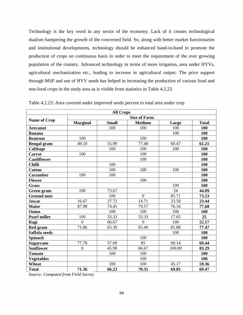
94
Technology is the key word in any sector of the economy. Lack of it creates technological
dualism hampering the growth of the concerned field. So, along with better market functionaries
and institutional developments, technology should be enhanced hand-in-hand to promote the
production of crops on continuous basis in order to meet the requirement of the ever growing
population of the country. Advanced technology in terms of more irrigation, area under HYVs,
agricultural mechanization etc., leading to increase in agricultural output. The price support
through MSP and use of HYV seeds has helped in increasing the production of various food and
non-food crops in the study area as is visible from statistics in Table 4.2.23.
Table 4.2.23: Area covered under improved seeds percent to total area under crop
All Crops
Name of Crop Size of Farm
Marginal Small Medium Large Total
Arecanut
100 100 100 100
Banana
100 100
Beatroot 100
100
100
Bengal gram 49.10 55.99 77.48 60.47 61.21
Cabbage
100 100 100 100
Carrot 100
100
100
Cauliflower
100
100
Chilli
100
100
Cotton
100 100 100 100
Cucumber 100 100
100
Flower
100
100
Grass
100 100
Green gram 100 73.67
24 44.09
Ground nuts
100 0 85.71 73.53
Jowar 16.67 37.72 14.71 23.58 23.44
Maize 87.98 74.45 79.57 76.16 77.68
Onion
100 100 100 100
Pearl millet 100 33.33 33.33 17.65 25
Ragi 0 66.67 0 100 52.17
Red gram 71.86 65.39 65.40 81.88 77.47
Saffola seeds
100 100
Spinach
100
100
Sugarcane 77.78 57.69 85 69.14 69.44
Sunflower 0 45.98 66.67 100.00 83.29
Tomato
100 100
100
Vegetables
100
100
Wheat
100 100 45.17 59.36
Total 71.36 66.23 70.35 69.85 69.47
Source: Computed from Field Survey

95
Among various crops grown, area mainly that of non-food crops was found to be under High
Yielding Variety (HYV) seeds. Area under cash crops, fuits and vegetables, fibers (cotton), and
some of the oilseeds like saffola-seeds, were found to be 100 percent under HYVs. The area
under HYV for sugarcane, sunflower and groundnut was 70, 83 and 76 percent, respectively. In
the case of pulses, 60 percent of the area on an average was sown under HYVs, with bengalgram
having 61 percent of area and redgram having 77 percent of area under purchased high yielding
seeds. Very less area (45 percent) of cereals was sown under HYVs except for maize which had
78 percent of area under HYV. The seed replacement ratio of non-food crops along with
sunflower, groundnut, wheat and three reference crops, viz., maize, redgram and bengalgram was
an indicator of technological awareness among sample farmers. This awareness needs to be
expanded to all the crops suitable for the respective area in order to increase their productivity
and production.
4.6 Regression Results of Marketed and Marketable Surplus
In order to accurately reflect the relationship between outcome variable and predictor variables
present in the data set, OLS regression was run on the same. The quantitative exercise was done
to identify factors that determine marketed/marketable surplus. Studies in the past carried out on
market surplus determinants were reviewed for the purpose. For example, Keya (1955) found
that among the various factors responsible for lowering marketed surplus for paddy in Assam,
lower volume of production, small size of holding, higher family size, lower irrigation facility
and lower area under high yield variety (HYV) were identified as crucial responsible factors. An
in-depth study conducted by Prasad (1989) for rice, wheat and maize in Bihar revealed that size
of holding, family size, income of households, irrigated area were the crucial factors that
determined marketed surplus. Another study by Chauhan and Amit (2005) found that production,
family size and average prices received by the farmers were the major factors responsible for a
significant impact on the size of marketed surplus for maize in Himachal Pradesh. Total
consumption, family size, off-farm income were identify as less important factors for
determining marketed surplus. Another empirical study by Kumar (2007) identified that value of
output, household size and area were the most significant factors responsible for marketed
surplus for wheat, paddy, pulsed and oilseeds in Haryana.

96
Based on the findings of above empirical studies, the variables which were taken into
consideration in order to form the model were: total production (qtls), net operated area (acres),
total retention (qtls), sale price ( ), distance (kms), loan per hectare ( ), family size per
household (numbers) and cost of storage ( per month) as predictors and marketed surplus as
the outcome variable of all the sample households. Before running the regression analysis,
correlation among the independent variables was examined, in order to check the inter-
correlation and to avoid the problem of multicolinearity among the variables. It was found that
there exists a very high correlation between production and quantity stored. So, the variable
quantity stored was dropped from the list of independent variables. The results with the selected
variables for respective crops are presented in Table 4.2.24a b c.
Table 4.2.24a: Regression result on marketed surplus for redgram
Dependent variable = Marketed output per acre (quintal)
Independent
variable
Coef. Std. Err. T P > t [95 percent
Conf.
Interval]
Prod (Qtl/Acre) 0.9275339 0.0159441 58.17 0.000 0.8959993 0.9590684
NCA (Acres) 0.0404018 0.0102662 3.94 0.000 0.020097 0.0607065
Sale Price (Rs/Qtl) -0.0001003 0.0001558 -0.64 0.521 -0.0004084 0.0002079
Loan per Acre 0.00000242 0.00000386 0.63 0.531 -0.00000521 0.0000101
Family size -0.0068001 0.0150804 -0.45 0.653 -0.0366266 0.0230263
Constant -0.1604136 0.5374707 -0.30 0.766 -1.223437 0.9026097
Number of observation 140
F (5, 134) = 712.07
Prob > F = 0.0000
R-squared = 0.9637
Adj R-squared = 0.9624
Root MSE = 0.518
Analyzing result for redgram, it can be observed from Table 4.2.24a that production was the
most important variable determining the value of marketed surplus. It had positive relation with
marketed surplus indicating higher production leads to higher marketed surplus. The coefficient
of production was around 0.93 indicating that one quintal increase in the production per acre
would increase the marketed surplus by 0.92 quintals per acre and it was significant at one
percent. Area was also significant at 5 percent indicating with increase in area under the crop
relatively higher proportion of output was marketed. The farmers who had taken loan marketed

97
higher amount of output. Sale price and family size had a negative relation with marketed surplus
but coefficients for both these variables were insignificant. The observed R-2 value was 0.96, that
indicates that the variation in dependent variable was well explained.
Table 4.2.24b: Regression result on marketed surplus for maize
Dependent variable = Marketed output per acre (quintal)
Mktd (Qtl/Acre) Coef. Std. Err. t P>t [95 percent Conf. Interval]
Prod (Qtl/Acre) 0.9368664 0.0524872 17.85 0.000 0.8330488 1.040684
NCA (Acres) 0.9347955 0.17287 5.41 0.000 0.5928653 1.276726
Sale Price (Rs/Qtl) 0.0035035 0.0049061 0.71 0.476 -0.0062006 0.0132076
Dist (Kms) 0.1493136 0.0594597 2.51 0.013 0.0317045 0.2669226
Loan per Acre 0.00000211 0.0000278 0.08 0.940 -0.0000529 0.0000571
Family size/HH -0.7388618 0.1367206 -5.40 0.000 -1.00929 -0.4684337
_cons -6.329662 5.656788 -1.12 0.265 -17.51857 4.859247
Number of observation 140
F (6, 133) = 61.16
Prob > F = 0.0000
R-squared = 0.7340
Adj R-squared = 0.7220
Root MSE = 5.0583
In the case of maize, production and area were the most important variables in determining
marketed surplus (Table 4.2.24b) both significant at one percent. The coefficient of sale price
indicated that a unit increase in sale price encourages the farmers to sell more. The coefficient of
distance was significant and positive that indicates a direct relation of distance with marketed
surplus which could be due to the lucrative prices offered by some of the agencies for which
farmers were ready to travel longer distances in order to sell their surplus amount. Indebtedness
also put pressure on the farmers to sell higher amount in the market probably to pay the loan
amount. The variable on family size was significant with a negative sign indicating that an extra
member in the family would decrease the marketed surplus. Among all the variables tired in the
regression equations, only sale price was found insignificant while loan amount was found
significant at 10 percent level whereas all other variable were significant at one percent level.
The R-2
value for maize was slightly less than that of redgram but still the variables on the right
hand side explain well on the left hand side.
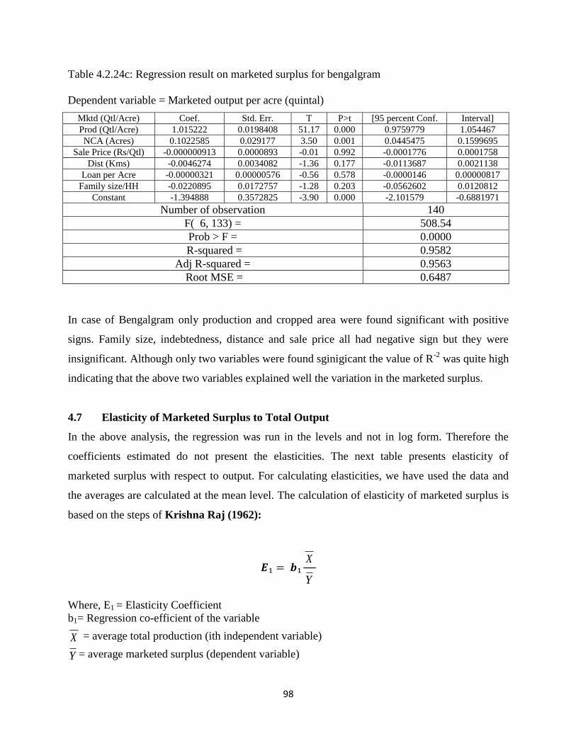
98
Table 4.2.24c: Regression result on marketed surplus for bengalgram
Dependent variable = Marketed output per acre (quintal)
Mktd (Qtl/Acre) Coef. Std. Err. T P>t [95 percent Conf. Interval]
Prod (Qtl/Acre) 1.015222 0.0198408 51.17 0.000 0.9759779 1.054467
NCA (Acres) 0.1022585 0.029177 3.50 0.001 0.0445475 0.1599695
Sale Price (Rs/Qtl) -0.000000913 0.0000893 -0.01 0.992 -0.0001776 0.0001758
Dist (Kms) -0.0046274 0.0034082 -1.36 0.177 -0.0113687 0.0021138
Loan per Acre -0.00000321 0.00000576 -0.56 0.578 -0.0000146 0.00000817
Family size/HH -0.0220895 0.0172757 -1.28 0.203 -0.0562602 0.0120812
Constant -1.394888 0.3572825 -3.90 0.000 -2.101579 -0.6881971
Number of observation 140
F( 6, 133) = 508.54
Prob > F = 0.0000
R-squared = 0.9582
Adj R-squared = 0.9563
Root MSE = 0.6487
In case of Bengalgram only production and cropped area were found significant with positive
signs. Family size, indebtedness, distance and sale price all had negative sign but they were
insignificant. Although only two variables were found sginigicant the value of R-2
was quite high
indicating that the above two variables explained well the variation in the marketed surplus.
4.7 Elasticity of Marketed Surplus to Total Output
In the above analysis, the regression was run in the levels and not in log form. Therefore the
coefficients estimated do not present the elasticities. The next table presents elasticity of
marketed surplus with respect to output. For calculating elasticities, we have used the data and
the averages are calculated at the mean level. The calculation of elasticity of marketed surplus is
based on the steps of Krishna Raj (1962):
X
Y
Where, E1 = Elasticity Coefficient
b1= Regression co-efficient of the variable
X = average total production (ith independent variable)
Y = average marketed surplus (dependent variable)
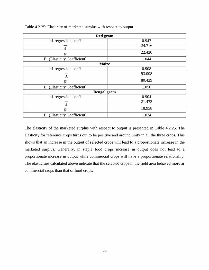
99
Table 4.2.25: Elasticity of marketed surplus with respect to output
Red gram
b1 regression coeff 0.947
X 24.716
Y 22.420
E1 (Elasticity Coefficient) 1.044
Maize
b1 regression coeff 0.908
X 93.008
Y 80.429
E1 (Elasticity Coefficient) 1.050
Bengal gram
b1 regression coeff 0.904
X 21.473
Y 18.958
E1 (Elasticity Coefficient) 1.024
The elasticity of the marketed surplus with respect to output is presented in Table 4.2.25. The
elasticity for reference crops turns out to be positive and around unity in all the three crops. This
shows that an increase in the output of selected crops will lead to a proportionate increase in the
marketed surplus. Generally, in staple food crops increase in output does not lead to a
proportionate increase in output while commercial crops will have a proportionate relationship.
The elasticities calculated above indicate that the selected crops in the field area behaved more as
commercial crops than that of food crops.

100
Chapter V
Concluding Observations and Policy Implications
5.1 Main Findings of the Study
The present study on marketed and marketable surplus is based on primary survey of four
districts of Karnataka while data available on the related variables over the years from various
secondary sources have also been analysed in the second chapter. The findings of the study are
summarized in the following paragraphs.
5.1.1 Findings from Secondary Data
Secondary data formed the basis on the overview of the foodgrains economy of the state. The
data collected over the years portrayed the trend in APY at the state and at all India level, growth
rate of three sectors, cropping pattern, and trend in consumption of major inputs like fertilizers,
farm mechanization, irrigation, HYVs etc. The findings from the secondary data are summarized
below:
Sectoral contribution to GSDP shows that among the three sectors, contribution of
service sector is the maximum, both at state and at all India level.
On an average, cereals contributed around 20 percent in Karnataka and 30 percent in
India towards total value of agricultural output as the area under the same has been
comparatively higher than other crops. Fruits and vegetables were also found to
contribute a larger share in the total value of whole agricultural output; 30 percent in
Karnataka and 25 percent in India.
Though cereals contribute the most towards agricultural value but area under the same
has been either declining or stagnating over the recent period as the growth rate of area
under cereals was 0.72 between 2001-02 and 2010-11 in Karnataka and 0.21 in India
during the same time period.
The share of area under various foodgrains though has been on the decline from past four
decades, yet area under foodgrains was recorded the highest with 61 percent of total area
in Karnataka and 64 percent in India. Among foodgrains, cereals held the majority
making 43 percent of the gross area in Karnataka and 52 percent of the gross area under

101
cereal crops in India during the period 2001-02 to 2010-11. Area under oilseeds has also
been on the rise from 12 to 18 percent in the state and 10 to 13 percent in the country.
The area increase in oilseeds was partly due to rising prices of oilseeds and partly
because of increase in their yield level, both played an incentive for the farmers to grow
more oilseeds.
Among our four selected districts and selected crops, Bijapur and Dharwad observed
around 20 percent growth in production of maize while Davangere and Gulbarga
observed around 6-7 percent growth in the 2000s. In all the four selected districts growth
was led more by area and less by the yield rate. In bengalgram, Bijapur and Gulbarga
observed very high growth rate in production in the 1990s but had significant negative
growth in the 2000s. Davangere observed positive growth in 2000s while Dharwad
observed positive growth in production in the 1990s. Production growth was a mixture of
area and yield led growth in different districts including the above mentioned selected
districts. In redgram, Gulbarga observed 16 percent growth in production in the 1990s
while Bijapur Dharwad observed around 20 percent growth in production in the 2000s.
Since more than 90 percent of the area of maize was under HYV in Karnataka compared
to only 35 percent area of all India, yield rate of maize in Karnataka was higher than all
India. All the three selected crops were rainfed in Karnataka as well as in the country as a
whole but among the three crops maize was better irrigated compared to bengalgram and
redgram.
The marketed surplus ratio of maize and redgram was much higher in Karnataka as
compared to all India. The increasing trends in Minimum Support Price and higher
consumption of fertilizer have helped in increasing the production of maize. Commercial
banks were the main source of agricultural credit to the farmers in Karnataka. Across
farm size groups, money lenders were the main source of lending for marginal farmers
whereas banks were ranked the main source of lending for the small, medium and large
farmers both at the state and at all India level.
The physical and financial estimates for tractors, power tillers and farm implements has
been recorded at a higher scale as investment in farm mechanization has increased by the
different farm size groups.
102
5.1.2 Findings from the Field Survey
The source of primary data for the study was field survey, which was conducted in the year
2012, for three crops- bengalgram, maize and redgram in the northern parts of Karnataka in four
selected districts namely – Belgaum, Bijapur, Davangere and Gulbarga. The questionnaire
included the details like area owned, net area sown, gross cropped area, area under various crops,
marketed surplus, marketable surplus, storage, total losses due to harvesting, winnowing,
threshing, transportation and storage, approximate present value of the farm machinery etc., and
the data was collected through personal canvassing by the project team in the field.
The study area was characterized by the dominance of pulses, particularly, redgram and
bengalgram while maize was the other major food crop grown in the study area. The study
makes use of 422 farm households selected from the above mentioned four districts of Karnataka
for the year 2012. Among 422 households 141 were redgram growers, 141 were bengalgram
growers and 140 grew maize, spread in four districts in the state of Karnataka. Among the
selected farmers, there were 89 marginal farmers, 143 small farmers, 84 medium farmers and
106 large farmers making a total sample of 422 farmers growing the above mentioned three
reference crops. The major findings of the primary survey are the following:
Agriculture was the main occupation of all the households and the age of the main
decision maker in the house was around 46 years on average. Farm labour was the
principal sub occupation of the farmers, especially the small and marginal farmers. The
average size of the family was around 6-7 members.
The respondents had attended 5-6 years of schooling, on average. Nearly 50 percent of
the respondents belonged to general category followed by OBCs and SCs/STs.
The net operated area of the selected households was 9.29 acres and gross cropped area
was 13.06 acres per household with a cropping intensity of 140.62. Main source of
irrigation was canal and tube well.
The cropping pattern of the selected farmers indicated that redgram, maize, bengalgram,
jowar and Cotton were the main crops grown by them. Karnataka is one of the largest
producers of redgram in the country and this crop was grown on 40.69 percent of GCA in
the study area. The area under redgram in cropping pattern increased with increase in
land holding size as 28.05 percent of area was under redgram cultivated by marginal

103
farmers which increased to 45.04 percent in the case of large farmers. Farmers used
HYVs for nearly 77 percent of area under redgram cultivation. Bengalgram was grown on
16.79 percent of GCA whereas maize was grown on 20 percent of total GCA. 78 percent
of area for maize was under HYV seeds and 61 percent of area of bengalgram was under
HYV seeds.
Going by three reference crops, 88.29 percent of bengalgram, 86.47 percent of maize and
90.71 percent of redgram was marketed out of total production. The rest amount was
retained by the households for their own consumption, seed, feed and for wages in kind.
In the case of bengalgram and redgram large farmers were the ones who produced the
maximum and the retention by them was also the highest. In the case of maize small
farmers retained more than other farm groups.
Out of the total produce of all the crops, 87.51 percent was marketed to various agencies,
9.22 percent was retained by the households for their own purpose while rest of the
amount was lost in harvesting and post harvesting. Transportation loss was 0.32 percent
of the total production whereas storage loss accounted for 2.95 percent of the total
production. High storage loss was due to the bad conditions of storage in the village.
The producer’s loss at the farm level for all the three crops was the highest in the case of
harvesting, as the mode of harvesting was mainly manua. The harvesting loss was
measured for bengalgram, 1.55 percent of total production, maize 3.03 percent of total
production and redgram 1.28 percent of the total production. The loss during threshing
for maize was the highest, 2.13 percent of total production whereas bengalgram and
redgram reported 0.95 percent and 0.90 percent loss of total production, respectively.
There was a decrease in loss during threshing due to the use of mechanical mode unlike
in harvesting. Only bengalgram and redgram reported to have had losses during
winnowing because of manual mode whereas the winnowing loss was zero for redgram
due to mechanical harvesting which does threshing automatically.
There was hardly any farmer who reported to have received subsidy of any kind. Besides,
the storage facility perceived was not adequate according to most of them. Creation of
additional storage was also not favored by most of them due to the non-accessibility of
the same.

104
Regarding channels of sale, most of the maize (72.27 percent) was sold in unregulated
market whereas major surplus of redgram (93.05 percent) was sold in the regulated
market. In the case of bengalgram, sale pattern to regulated and unregulated market was
around equal proportion, i.e., 50.83 percent in the regulated markets and 49.17 percent in
unregulated markets.
Due to the sale in unregulated markets, the average transportation cost was the least for
maize – Rs.13.88 per quintal and it was highest for redgram – Rs.39.82 per quintal due to
its sale in the regulated market that happens to be a place distant from the production
centre. For bengalgram it was nearly the average of above two crops – Rs.28.63 per
quintal.
There were very few farmers who knew about warehouse receipt programme, contract
farming and futures trading. Farmers were also not well aware about the minimum
support price system.
The farmers indicated selling more produce if the price realization is increased either by
keeping less for seed and feed or by changing their consumption pattern.
Good access to institutional credit indicates that the farmers were well aware about the
credit facilities available through banks and other institutions. Cooperative society was
the main source of credit due to low rate of interest along with commercial banks where
the rate of interest was higher than cooperatives but far less than the non institutional
sources.
Due to increase in financial literacy, around 1/3rd
of the farmers among the selected
households possessed Kisan Credit Card with a credit limit not exceeding 1.25 lakh.
Traders and Agricultural Produce Market Committees were the main sources of price
information for the farmers with a little contribution from telephonic conversation and
visits to the market.
The quantitative analysis indicated that net operated area, sale price, family size, loan per
acre and distance explained the marketed surplus to some extent but it was production
that had a major impact on marketed surplus of all the three crops. The unit elasticity of
marketed surplus with respect to output of all the three crops substantiated the above
findings that with increase in output there was a proportionate increase in marketed
surplus.

105
5.2 Policy Implications
In order to increase the marketed surplus of various crops major steps have been taken up by the
state and the centre, but the inclusiveness of the programmes is hardly seen which causes a
loophole in the entire process. Keeping in view above cited conclusions, the following
suggestions could be perceived in better implementation of the policies.
Scientific godowns should be constructed in the rural areas making storage facility better
and accessible to all and preventing crop loss due to lack of storage facility.
More number of APMCs should be set up near the village area with good pricing policy
to reduce the transportation loss and to deal with the problem of middlemen.
Government should take up the responsibility of educating the farmers about pricing
policy, fertilizers, machineries, manures, centrally sponsored schemes, credit facilities,
etc by organizing awareness/training programmes at regular intervals in nearby areas.
The training programmes in the state could facilitate information to farmers about
existing agriculture departments that provide details on-line like: Bhoomi (online delivery
and management of land records in Karnataka), Department of Agriculture
(raitamitra.kar.nic.in), Krishi Marata Vahini (online agriculture price information system
on daily basis) etc.
Inclusion of new technology, coordination and investment in infrastructure from field to
consumption are critical for reducing losses.
State government introduced interest free short-term crop loans up to 1 lakh for farmers
in the budget during 2012-13 and the same proposal has been carried in the budget 2013-
14. The provision of loan should be made accessible to all groups of farmers since 75
percent of farmers in the state are marginal and small. High cost of farm equipments and
scarcity of agricultural labourers makes it difficult for such farmers to carry on
agricultural operations timely.
In order to throw more light on composite problems of production and of marketed and
marketable surplus with an integrated perspective, the focus should be on the data record
not only with respect to production and costs but also giving equal importance to data
related to quantities marketed, costs of marketing, prices obtained after sale, and non-
market disposals as well as on the quality of the produce sold.

106
REFERENCES
Adesiyan O.F., Adesiyan A.T., Oluitan R.O., (2012), Market Supply Response of Cassava
Farmers in Ile-Ife, Osun State, CSCanada-Canadian Social Sciences, Vol.8, No.3,
pp.61-63.
Aiyasami U. and Bhole H.G., (March 28, 1981), Market Access as constraint on Marginal
and Small Farmers, Economic and Political Weekly, Vol.16, No.13, pp. A29 + A31 +
A33 – A36
Chauhan S.K., and Chhabra Amit ( 2005) Marketable surplus and prices-spread for maize in
Hamirput district of Himachal Pradesh, Agricultural Economics Research Review,
vol no, 18, Jan-June, 2005, PP 39-49.
Hati Ashok, (July 17, 1976), Non-Linear Marketable Surplus Functions, Economic and
Political Weekly, Vol.11, No.29, pp 1080-1084.
Kumar, Parmod (2007), Farm size and marketing efficiency: pre and post lierlization,
Concept Publication, New Delhi.
Nadkarni M.V. (March 29, 1980), Marketable Surplus and Market Dependence: A Millet
Region of Maharashtra, Economic and Political Weekly, Vol.15, No.13, pp. A13-
A15 + A17-A19 + A21-A24
Prabha T. (Dec 22-29, 1984), Government Intervention and Marketed Surplus Disposal: A
Case Study of Tamil Nadu, Economic and Political Weekly, Vol.19, No.51/52, pp.
2171 + 2173 – 2175.
Prasad Jagdish, Marketable Surplus and Market Performance: A Study with Special
Reference to Muzaffar Foodgrain Market in Bihar – First Edition, 1989; Mittal
Publications, 4528/12.
Reports from Directorate of Economics and Statistics, Ministry of Agriculture, Government
of India.
Rudra Asok and Madan Mohan Mukhopadhyay (July 7, 1973), Marketing Behaviour of Big,
Medium and Small farmers, Economic and Political Weekly, Vol.8, No.27, pp 1199-
1202.
Sengupta, Keya (1955), Determinats of marketed surplus in a backward Economy: a case
study of three districts of south Assam.
Upender, M. (1992), Marketable and Marketed Surplus in Agriculture, Economic and
Political Weekly, Vol.27, No.28, July 11, pp.1476

107
WEBLINKS:
http://en.wikipedia.org/wiki/List_of_districts_of_Karnataka
http://en.wikipedia.org/wiki/Agriculture_in_India#Problems
http://www.jstor.org
http://joeleebass.hubpages.com/hub/17-problems-of-agricultural-development
http://www.alc.gov.bc.ca/publications/planning/Planning_for_Agriculture/Chapter09/090
24reference.htm
http://www.agricultureinformation.com/mag/2008/02/department-of-agricultural-
marketing-karnataka-state-agricultural-marketing-board/
http://www.indiaagronet.com/indiaagronet/Agri_marketing/contents/regulated_markets.h
tm
http://www.thehindubusinessline.com/news/states/karnataka-agriculture-budget-lays-stress-on-
marketing-facilities/article4393920.ece
http://socialprotectioncommunity.in/2012/12/the-growth-of-organic-agriculture-in-karnataka/
http://bjpkarnataka.org/communication-cell/karnataka-bjp-government-introduced-interest-free-
loans-up-to-rs-1-lakh-for-farmers-in-budget-2012-13/
http://news.oneindia.in/2012/03/21/karnataka-budget-2012-zero-interest-on-crop-loans.html
http://books.google.co.in/books?id=AdUleFZhkugC&pg=PA65&lpg=PA65&dq=determi
ning+marketed+surplus+by+sengupta&source=bl&ots=a7LlHSqQs6&sig=FL7SoeeihIfY
z9_eBoaMdZDY3H0&hl=en&sa=X&ei=gAq4UaaFE83JrAea7oCICA&ved=0CDYQ6A
EwAQ

108
Review Report
1. Title of the Draft Study Report Examined: Assessment of Marketed and Marketable Surplus of
Foodgrain Crops in Karnataka
2. Date of Receipt of the Draft Report: July 29, 2013
3. Date of Despatch of Comments: October 31, 2013
4. Comments on the Objectives of the study: The objectives are attended by the report.
5. Comments on the Methodology: The report has examined the issue with coverage of three crops
across four districts. But, the sampling of farmer households does not seem to be representative of
average land holding profile of the state or the study districts. Also, semi-medium category is
completely missing and no reason has been given for merging it with medium category. It is not
possible that only 20% farmers in the state are marginal. The 2000-01 data show that 48% farmers in
Karnataka were marginal and 27% small. Further, 40% of the total farmers in Belgaum were
marginal and 20% small. Therefore, sample seems biased against marginal farmers.
6. Overall View on Acceptability of the Report:
1. The organisation of the report is poor as many parts are either missing or misplaced. For example,
the review should have come before objectives and methodology but is put later and stands alone
without any summary of major aspects covered and research gaps.
2. The chapter scheme given in first chapter (p. 6 and 7) is repeated in chapter 2 (p. 20).
3. No reference is given for German Scientist quoted on p. 39.
4. Chapter 3 has no details at all of farmer land holding either state level or district levels which is
surprising as that is the most crucial determinant of marketable surplus and the sampling of the study
is supposed to be based on that.
5. Table 4.2 2 should also give %ages in total for all categories and districts.
6. Reference list is poorly complied which needs to be corrected and reference given professionally.
After it is revised based on some of these comments, the report can be accepted.
109
Action Taken by the Author - ADRTC Bangalore
Based on the comments on the draft report, Assessment of Marketed and Marketable Surplus
of Food grains Crops in Karnataka received from the Centre for Management in Agriculture
(CMA), Indian Institute of Management (IIM) Ahmedabad, the report has been revised. With
respect to methodology, as per instruction given by the CMA, the farmers were selected based on
principal crop and not on household basis. The condition was to have at least 20 farmers in each
category for every principal crop and that criterion was adhered to while making the selection of
the farmers. The four category of marginal, small, medium and large were kept as per
Agriculture Census definition. However, due representation was given to all categories. The
organization of the study has been changed keeping the referee report in mind. The land details
district wise are provided in Table 4.1.8 and cropping pattern is provided in Table 4.1.11.
Missing references are given. The draft has been rechecked and all the corrections are made in
the final report.