arX

iv:1

312.

5934

v1 [

stat

.ME

] 2

0 D

ec 2

013

Statistical Science

2013, Vol. 28, No. 4, 510–520DOI: 10.1214/13-STS440c© Institute of Mathematical Statistics, 2013

Assessment of Point Process Models forEarthquake ForecastingAndrew Bray and Frederic Paik Schoenberg

Abstract. Models for forecasting earthquakes are currently tested pro-spectively in well-organized testing centers, using data collected afterthe models and their parameters are completely specified. The extentto which these models agree with the data is typically assessed using avariety of numerical tests, which unfortunately have low power and maybe misleading for model comparison purposes. Promising alternativesexist, especially residual methods such as super-thinning and Voronoiresiduals. This article reviews some of these tests and residual methodsfor determining the goodness of fit of earthquake forecasting models.

Key words and phrases: Earthquakes, model assessment, point pro-cess, residual analysis, spatial–temporal statistics, super-thinning.

1. INTRODUCTION

A major goal in seismology is the ability to accu-rately anticipate future earthquakes before they oc-cur (Bolt (2003)). Anticipating major earthquakesis especially important, not only for short-term re-sponse such as preparation of emergency personneland disaster relief, but also for longer-term prepa-ration in the form of building codes, urban plan-ning and earthquake insurance (Jordan and Jones(2010)). In seismology, the phrase earthquake pre-

diction has a specific definition: it is the identifi-cation of a meaningfully small geographic regionand time window in which a major earthquake willoccur with very high probability. An example ofearthquake predictions are those generated by theM8 method (Keilis-Borok and Kossobokov (1990)),which issues an alarm whenever there is a suitablylarge increase in the background seismicity of a re-gion. Such alarms could potentially be very valuable

Andrew Bray is Ph.D. Student and Frederic Paik

Schoenberg is Professor, UCLA, Department of

Statistics, 8125 Math Sciences Building, Los Angeles,

California 90095-1554, USA.

This is an electronic reprint of the original articlepublished by the Institute of Mathematical Statistics inStatistical Science, 2013, Vol. 28, No. 4, 510–520. Thisreprint differs from the original in pagination andtypographic detail.

for short-term disaster preparedness, but unfortu-nately examples of M8-type alarms, including thenotable Reverse Tracing of Precursors (RTP) algo-rithm, have generally exhibited low reliability whentested prospectively, typically failing to outperformnaive methods based simply on smoothed historicalseismicity (Geller et al. (1997); Zechar and Jordan(2008)).Earthquake prediction can be contrasted with the

related earthquake forecasting, which means the as-signment of probabilities of earthquakes occurringin broader space–time-magnitude regions. The tem-poral scale of an earthquake forecast is more on parwith climate forecasts and may be over intervals thatrange from decades to centuries (Hough (2010)).Many models have been proposed for forecasting

earthquakes, and since different models often resultin very different forecasts, the question of how toassess which models seem most consistent with ob-served seismicity becomes increasingly important.Concerns with retrospective analyses, especially re-garding data selection, overfitting and lack of repro-ducibility, have motivated seismologists recently tofocus on prospective assessments of forecasting mod-els. This has led to the development of the RegionalEarthquake Likelihood Models (RELM) and Collab-orative Study of Earthquake Predictability (CSEP)testing centers, which are designed to evaluate andcompare the goodness of fit of various earthquake

1

2 A. BRAY AND F. P. SCHOENBERG

forecasting models. This paper surveys methods forassessing the models in these RELM and CSEP ex-periments, including methods currently used byRELM and CSEP and some others not yet in usebut which seem promising.

2. A FRAMEWORK FOR PROSPECTIVE

TESTING

The current paradigm for building and testingearthquake models emerged from the working groupfor the development of Regional Earthquake Likeli-hood Models (RELM) in 2001. As described in Field(2007), the participants were encouraged to submitdiffering models, in the hopes that the competitionbetween models would prove more useful than tryingto build a single consensus model. The competitiontook place within the framework of a prospectivetest of their seismicity forecasts. Working from astandardized data set of historical seismicity, scien-tists fit their models and submit to RELM a fore-cast of the number of events expected within eachof many pre-specified spatial–temporal-magnitudebins. The first predictive experiment required mod-els to forecast seismicity in California between 2006to 2011 using only data from before 2006.This paradigm has many benefits from a statisti-

cal perspective. The prospective nature of the exper-iments effectively eliminates concerns about overfit-ting. Furthermore, the standardized nature of thedata and forecasts facilitates the comparison amongdifferent models. RELM has since expanded intothe Collaborative Study of Earthquake Predictabil-ity (CSEP), a global-scale project to coordinate mod-el development and conduct prospective testing ac-cording to community standards (Jordan (2006)).CSEP serves as an independent entity that providesstandardized seismicity data, inventories proposedmodels and publishes the standards by which themodels will be assessed.

3. SOME EXAMPLES OF MODELS FOR

EARTHQUAKE OCCURRENCES

The first predictive experiment coordinatedthrough RELM considered time-independent spatialpoint process models, which can be specified by theirPapangelou intensity λ(s), a function of spatial loca-tion s. A representative example is the model speci-fied by Helmstetter, Kagan and Jackson (2007) that

is based on smoothing previous seismicity. The in-tensity function is estimated with an isotropic adap-tive kernel

λ(s) =N∑i=1

Kd(s− si),

where N is the total number of observed points, andKd is a power-law kernel

Kd(s− si) =C(d)

(|s− si|2 + d2)1.5,

where d is the smoothing distance, C(d) is a normal-izing factor so that the integral of Kd(·) over an infi-nite area equals 1, and | · | is the Euclidean norm. Theestimated number of points within the pre-specifiedgrid cells is obtained by integrating λ(s) over eachcell.Models of earthquake occurrence that consider it

to be a time-dependent process are commonly vari-ants of the epidemic-type aftershock sequence (ETAS)model of Ogata (1988, 1998) (see, e.g., Helmstetterand Sornette (2003); Ogata, Jones and Toda, 2003;Sornette (2005); Vere-Jones and Zhuang (2008); Con-sole, Murru and Falcone, 2010; Chu et al. (2011);Wang, Jackson and Kagan, 2011; Werner et al. (2011);Zhuang (2011); Tiampo and Shcherbakov (2012)).According to the ETAS model, earthquakes causeaftershocks, which in turn cause more aftershocks,and so on. ETAS is a point process model speci-fied by its conditional intensity, λ(s, t), which repre-sents the infinitesimal expected rate at which eventsare expected to occur around time t and location s,given the history Ht of the process up to time t.ETAS is a special case of the linear, self-excitingHawkes’ point process (Hawkes (1971)), where theconditional intensity is of the form

λ(s, t|Ht) = µ(s, t) +∑ti<t

g(s− si, t− ti;Mi),

where µ(s, t) is the mean rate of a Poisson-distributedbackground process that may in general vary withtime and space, g is a triggering function whichindicates how previous occurrences contribute, de-pending on their spatial and temporal distances andmarks, to the conditional intensity λ at the locationand time of interest, and (si, ti,Mi) are the origintimes, epicentral locations and moment magnitudesof observed earthquakes.Ogata (1998) proposed various forms for the trig-

gering function, g, such as the following:

g(s, t,M) =K(t+ c)−pea(M−M0)(|s|2 + d)−q,

EARTHQUAKE MODEL ASSESSMENT 3

where M0 is the lower magnitude cutoff for the ob-served catalog.The parameters in ETAS models and other spatial–

temporal point process models may be estimated bymaximizing the log-likelihood,

n∑i=1

log{λ(si, ti)} −∫S

∫λ(s, t)dsdt.

The maximum likelihood estimator (MLE) of apoint process is, under quite general conditions,asymptotically unbiased, consistent, asymptoticallynormal and asymptotically efficient (Ogata (1978)).Finding the parameter vector that maximizes thelog-likelihood can be achieved using any of the vari-ous standard optimization routines, such as the quasi-Newton methods implemented in the functionoptim(·) in R. The spatial background rate µ inthe ETAS model can be estimated in various ways,such as via kernel smoothing seismicity from priorto the observation window or kernel smoothing thelargest events in the catalog, as in Ogata (1998)or Schoenberg (2003). Note that the integral termin the loglikelihood function can be cumbersometo estimate, and an approximation method recom-mended in Schoenberg (2013) can be used to accel-erate computation of the MLE.There are of course many other earthquake fore-

casting models quite distinct from the two point pro-cess models above. Perhaps most important amongthese are the Uniform California Earthquake Rup-ture Forecast (UCERF) models, which are consultedwhen setting insurance rates and crafting buildingcodes (Field et al. (2009)). They are constructed bysoliciting expert opinion from leading seismologistson which components should enter the model, howthey should be weighted, and how they should inter-act (Marzocchi and Zechar (2011)). Examples of thecomponents include slip rate, geodetic strain ratesand paleoseismic data. Note that some seismologistshave argued that evaluating some earthquake fore-casting models such as UCERF using model vali-dation experiments such as RELM and CSEP maybe inappropriate, though such a conclusion seems torun counter to basic statistical and scientific princi-ples.Although the UCERF models draw upon diverse

information related to the geophysics of earthquakeetiology, commonly used models such as ETAS andits variants rely solely on previous seismicity forforecasting future events. Many attempts have been

made to include covariates, but when assessed rigor-ously, most predictors other than the locations andtimes of previous earthquakes have been shown notto offer any noticeable improvement in forecasting.Recent examples of such covariates include electro-magnetic signals (Jackson (1996); Kagan (1997)),radon (Hauksson and Goddard (1981)) and waterlevels (Bakun et al. (2005); Manga andWang (2007)).A promising exception is moment tensor informa-tion, which is now routinely recorded with each earth-quake and seems to give potentially useful informa-tion regarding the directionality of the release ofstress in each earthquake. However, this informa-tion appears not to be explicitly used presently inmodels in the CSEP or RELM forecasts.

4. NUMERICAL TESTS

Several numerical tests were initially proposed toserve as the metrics by which RELM models wouldbe evaluated (Schorlemmer et al. (2007)). For thesenumerical tests, each model consists of the estimatednumber of earthquakes in each of the spatial–tempo-ral-magnitude bins, where the number of events ineach bin is assumed to follow a Poisson distributionwith an intensity parameter equivalent to the fore-casted rate.The L-test (or Likelihood test) evaluates the prob-

ability of the observed data under the proposed mod-el. The numbers of observed earthquakes in eachspatial–temporal-magnitude bin are treated as inde-pendent random variables, so the joint probabilityis calculated simply as the product of their corre-sponding Poisson probabilities. This observed jointprobability is then considered with respect to thedistribution of joint probabilities generated by sim-ulating many synthetic data sets from the model.If the observed probability is unusually low in thecontext of this distribution, the data are consideredinconsistent with the model.TheN -test (Number) ignores the spatial and mag-

nitude component and focuses on the total numberof earthquakes summed across all bins. If the pro-posed model provides estimates λi for i correspond-ing to each of B bins, then according to this model,the total number of observed earthquakes shouldbe Poisson distributed with mean (

∑Bi=1 λi). If the

number of observed earthquakes is unusually largeor small relative to this distribution, the data areconsidered inconsistent with the model.

4 A. BRAY AND F. P. SCHOENBERG

The L-test is considered more comprehensive inthat it evaluates the forecast in terms of magni-tude, spatial location and number of events, whilethe N -test restricts its attention to the number ofevents. Two additional data consistency tests wereproposed to assess the magnitude and spatial com-ponents of the forecasts, respectively: the M -testand the S-test (Zechar, Gerstenberger and Rhoades,2010). The M -test (Magnitude) isolates the fore-casted magnitude distribution by counting the ob-served number of events in each magnitude bin with-out regard to their temporal or spatial locations,standardized so that the observed and expected to-tal number of events under the model agree, andcomputing the joint (Poisson) likelihood of the ob-served numbers of events in each magnitude bin. Aswith the L-test, the distribution of this statistic un-der the forecast is generated via simulation.The S-test (Spatial) follows the same inferential

procedure but isolates the forecasted spatial distri-bution by summing the numbers of observed eventsover all times and over all magnitude ranges. Thesecounts within each of the spatial bins are again stan-dardized so that the observed and expected totalnumber of events under the model agree, and thenone computes the joint (Poisson) likelihood of theobserved numbers of events in the spatial bins.The above tests measure the degree to which the

observations agree with a particular model, in termsof the probability of these observations under thegiven model. As noted in Zechar et al. (2013), testssuch as the L-test and N -test are really tests ofthe consistency between the data and a particularmodel, and are not ideal for comparing two models.Schorlemmer et al. (2007) proposed an additionaltest to allow for the direct comparison of the perfor-mance of two models: the Ratio test (R-test). For acomparison of models A and B, and given the num-bers of observed events in each bin, the test statisticR is defined as the log-likelihood of the data ac-cording to model A minus the corresponding log-likelihood for model B. Under the null hypothesisthat model A is correct, the distribution of the teststatistic is constructed by simulating from model Aand calculating R for each realization. The resultingtest is one-sided and is supplemented with the corre-sponding test using model B as the null hypothesis.The T -test and W -test of Rhoades et al. (2011) arevery similar to the R-test, except that instead of us-ing simulations to find the null distribution of thedifference between log-likelihoods, with the T -test

and W -test, the differences between log-likelihoodswithin each space–time-magnitude bin for models Aand B are treated as independent normal or sym-metric random variables, respectively, and a t-testor Wilcoxon signed rank test, respectively, is per-formed.Unfortunately, when used to compare various mod-

els, such likelihood-based tests suffer from the prob-lem of variable null hypotheses and can lead to highlymisleading and even seemingly contradictory results.For instance, suppose model A has a higher like-lihood than model B. It is nevertheless quite pos-sible for model A to be rejected according to theL-test and model B not to be rejected using theL-test. Similarly, the R-test with model A as thenull might indicate that model A performs statis-tically significantly better than model B, while theR-test with model B as the null hypothesis may indi-cate that the difference in likelihoods is not statisti-cally significant. Seemingly paradoxical results likethese occur frequently, and at a recent meeting ofthe Seismological Society of America, much confu-sion was expressed over such results; even some seis-mologists quite well versed in statistics referred toresults in such circumstances as “somewhat mixed,”even though model A clearly fit better according tothe likelihood criterion than model B.The explanation for such results is that the null

hypotheses of the two tests are different: when mod-el A is tested using the L-test, the null hypothesisis model A, and when model B is tested, the nullhypothesis is model B. The test statistic may havevery different distributions under these different hy-potheses.Unfortunately, these types of discrepancies seem

to occur frequently and hence, the results of thesenumerical tests may not only be uninformative formodel comparison, but in fact highly misleading.A striking example is given in Figure 4 of Zecharet al. (2013), where the Shen, Jackson and Kagan(2007) model produces the highest likelihood of thefive models considered in this portion of the analysis,and yet under the L-test has the lowest correspond-ing p-value of the five models.

5. FUNCTIONAL SUMMARIES

Functional summaries, that is, those producing afunction of one variable, such as the weighted K-function and error diagrams, can also be useful mea-sures of goodness of fit. However, such summaries

EARTHQUAKE MODEL ASSESSMENT 5

typically provide little more information than nu-merical tests in terms of indicating where and whenthe model and the data fail to agree or how a modelmay be improved.The weighted K-function is a generalized version

of the K-function of Ripley (1976), which has beenwidely used to detect clustering or inhibition forspatial point processes. The ordinary K function,K(h), counts, for each h, the total number of ob-served pairs of points within distance h of one an-other, per observed point, standardized by divid-ing by the estimated overall mean rate of the pro-cess, and the result is compared to what would beexpected for a homogeneous Poisson process. Theweighted version, Kw(h), was introduced for the in-homogeneous spatial point process case by Badde-ley, Møller and Waagepetersen (2000), and is de-fined similarly to K(h), except that each pair of

points (si, sj) is weighted by 1/[λ(si)λ(sj)], the in-verse of the product of the modeled unconditionalintensities at the points si and sj . This was ex-tended to spatial–temporal point processes by Veenand Schoenberg (2006) and Adelfio and Schoenberg(2009).Whereas the null hypothesis for the ordinary K-

function is a homogeneous Poisson process, in thecase of Kw, the weighting allows one to assesswhether the degree of clustering or inhibition in theobservations is consistent with what would be ex-pected under the null hypothesis corresponding tothe model for λ. While weighted K-functions maybe useful for indicating whether the degree of clus-tering in the model agrees with that in the obser-vations, such summaries unfortunately do not ap-pear to be useful for comparisons between multiplecompeting models, nor do they accurately indicatein which spatial–temporal-magnitude regions theremay be particular inconsistencies between a modeland the observations.Error diagrams, which are also sometimes called

receiver operating characteristic (ROC) curves(Swets (1973)) or Molchan diagrams (Molchan(1991), 2010; Zaliapin and Molchan (2004); Kagan(2009)), plot the (normalized) number of alarms ver-sus the (normalized) number of false negatives (fail-ures to predict), for each possible alarm, where inthe case of earthquake forecasting models an alarm

is defined as any value of the modeled conditionalrate, λ, exceeding some threshold. Figure 1 presentserror diagrams for two RELM models, Helmstetter,Kagan and Jackson (2007) and Shen, Jackson and

Fig. 1. Error diagrams for Helmstetter, Kagan and Jack-son (2007) in blue and Shen, Jackson and Kagan (2007) inorange. Model details are in Sections 3 and 7, respectively.

Kagan (2007) (see Sections 3 and 7 for model de-tails).The ease of interpretation of such diagrams is an

attractive feature, and plotting error diagrams withmultiple models on the same plot can be a useful wayto compare the models’ overall forecasting efficacy.In Figure 1 we learn that Shen, Jackson and Kagan(2007) slightly outperforms Helmstetter, Kagan andJackson (2007) when the threshold for the alarm ishigh, but as the threshold is lowered Helmstetter,Kagan and Jackson (2007) performs noticeably bet-ter. For the purpose of comparing models, one mayeven consider normalizing the error diagram so thatthe false negative rates are considered relative toone of the given models in consideration as in Ka-gan (2009). This tends to alleviate a common prob-lem with error diagrams as applied to earthquakeforecasts, which is that most of the relevant focusis typically very near the axes and thus it can bedifficult to inspect differences between the modelsgraphically. A more fundamental problem with er-ror diagrams, however, is that while they can beuseful overall summaries of goodness of fit, such di-agrams unfortunately provide little information asto where models are fitting poorly or how they maybe improved.

6. RESIDUAL METHODS

Residual analysis methods for spatial–temporalpoint process models produce graphical displays which

6 A. BRAY AND F. P. SCHOENBERG

may highlight where one model outperforms anotheror where a particular model does not ideally agreewith the data. Some residual methods, such as thin-ning, rescaling and superposition, involve transform-ing the point process using a model for the condi-tional intensity λ and then inspecting the unifor-mity of the result, thus reducing the difficult prob-lem of evaluating the agreement between a possiblycomplex spatial–temporal point process model anddata to the simpler matter of assessing the homo-geneity of the residual point process. Often, depar-tures from homogeneity in the residual process canbe inspected by eye, and many standard tests arealso available. Other residual methods, such as pixelresiduals, Voronoi residuals and deviance residuals,result in graphical displays that can quite directlyindicate locations where a model appears to departfrom the observations or where one model appearsto outperform another in terms of agreement withthe data.

6.1 Thinned, Superposed and Super-Thinned

Residuals

Thinned residuals are based on the technique ofrandom thinning, which was first introduced byLewis and Shedler (1979) and Ogata (1981) for thepurpose of simulating spatial–temporal point pro-cesses and extended for the purpose of model eval-uation in Schoenberg (2003). The method involveskeeping each observed point (earthquake) indepen-

dently with probability b/λ(si, ti), where b =

inf(s,t)∈S{λ(s, t)} and λ is the modeled conditionalintensity. If the model is correct, that is, if the es-timate λ(s, t) = λ(s, t) almost everywhere, then theresidual process will be homogeneous Poisson withrate b (Schoenberg (2003)). Because the thinning israndom, each thinning is distinct, and one may in-spect several realizations of thinned residuals andanalyze the entire collection to get an overall assess-ment of goodness of fit, as in Schoenberg (2003).An antithetical approach was proposed by Bre-

maud (1981), who suggested superposing a simu-lated point process onto an observed point processrealization so as to yield a homogeneous Poissonprocess. As indicated in Clements, Schoenberg andVeen (2012), tests based on thinned or superposed

residuals tend to have low power when the model λfor the conditional intensity is volatile, which is typi-cally the case with earthquake forecasts since earth-quakes tend to be clustered in particular spatial–temporal regions. Thinning a point process will lead

to very few points remaining if the infimum of λ overthe observed space is small (Schoenberg (2003)),while in superposition, the simulated points, whichare by construction approximately homogeneous, willform the vast majority of residual points if the supre-mum of λ is large.A hybrid approach called super-thinning was in-

troduced in Clements, Schoenberg and Veen (2012).With super-thinning, a tuning parameter k is cho-sen, and one thins (deletes) the observed points in

locations of space–time where λ > k, keeping eachpoint independently with probability k/λ(s, t), and

superposes a Poisson process with rate λ(s, t)/k

where λ < k. When the tuning parameter k is cho-sen wisely, the method appears to be more powerfulthan thinning or superposing in isolation.

6.2 Rescaled Residuals

An alternative method for residual analysis is re-scaling. The idea behind rescaled residuals datesback to Meyer (1971), who investigated rescalingtemporal point processes according to their condi-tional intensities, moving each point ti to a new time∫ ti0 λ(t)dt, creating a transformed space in whichthe rescaled points are homogeneous Poisson of unitrate. Heuristically, the space is essentially compressedwhen λ is small and stretched when λ is large, sothat the points are ultimately uniformly distributedin the resulting transformed space, if the model forλ is correct. This method was used in Ogata (1988)to assess a temporal ETAS model and extended inMerzbach and Nualart (1986), Nair (1990), Schoen-berg (1999) and Vere-Jones and Schoenberg (2004)to the spatial and spatial–temporal cases. Rescalingmay result in a transformed space that is difficult toinspect if λ varies widely over the observation region,and in such cases standard tests of homogeneity suchas Ripley’sK-function may be dominated by bound-ary effects, as illustrated in Schoenberg (2003).

6.3 Pixel Residuals

A different type of residual analysis which is moreclosely analogous to standard residual methods inregression or spatial statistics is to consider the (stan-dardized) differences between the observed and ex-pected numbers of points in each of various spa-tial or spatial–temporal pixels or grids, producingwhat might be called pixel residuals. These types ofresiduals were described in great detail by Baddeleyet al. (2005) and Baddeley, Møller and Pakes (2008).More precisely, the raw pixel residual on each pixel

EARTHQUAKE MODEL ASSESSMENT 7

Ai is defined as N(Ai)−∫λ(s, t)dtds, where N(Ai)

is simply the number of points (earthquakes) ob-served in pixel Ai (Baddeley et al. (2005)). Baddeleyet al. (2005) also proposed various standardizationsincluding Pearson residuals, which are scaled in re-lation to the standard deviation of the raw residuals:

ri =N(Ai)−

∫λ(s,t)dtds√∫

λ(s,t)dtds.

A problem expressed in Bray et al. (2014) is thatif the pixels are too large, then the method is notpowerful to detect local inconsistencies between themodel and data, and places in the interior of a pixelwhere the model overestimates seismicity may can-cel out with places where the model underestimatesseismicity. On the other hand, if the pixels are small,then the majority of the raw residuals are close tozero while those few that correspond to pixels withan earthquake are close to one. In these situationswhere the residuals have a highly skewed distribu-tion, the skew is only intensified by the standardiza-tion to Pearson residuals. As a result, plots of boththe raw and the Pearson residuals are not informa-tive and merely highlight the pixels where earth-quakes occur regardless of the fit of the model. Theraw or Pearson residuals may be smoothed, as inBaddeley et al. (2005), but such smoothing typi-cally only reveals gross, large-scale inconsistenciesbetween the model and data.If one is primarily interested in comparing com-

peting models, then instead one may plot, in eachpixel, the difference between log-likelihoods for thetwo models, as in Clements, Schoenberg and Schor-lemmer (2011). The resulting residuals may be calleddeviance residuals, in analogy with residuals from lo-gistic regression and other generalized linear models.Deviance residuals appear to be useful for compar-ing models on grid cells and inspecting where onemodel appears to fit the observed earthquakes bet-ter than the other. It remains unclear how theseresiduals may be used or extended to enable com-parisons of more than two competing models, otherthan by comparing two at a time.

6.4 Voronoi Residuals

One method of addressing the problem of pixelsize specification is to use a data-driven, spatiallyadaptive partition such as the Voronoi tessellation,as suggested in Bray et al. (2014). Given n observedearthquakes, one may obtain a collection of n Voronoicells A1, . . . ,An, where Ai is defined as the collection

of spatial–temporal locations closer to the particu-lar point (earthquake) i than to any of the other ob-served points (Okabe et al. (2000)). Thus,N(Ai) = 1for each cell Ai. One may then compute the cor-

responding standardized residuals ri =1−

∫λ(s,t)dtds√∫λ(s,t)dtds

over the Voronoi cells Ai. As with pixel residuals,for each Voronoi cell one may choose to plot the rawresidual, or the residual deviance if one is interestedin comparing competing models. Voronoi residualsare shown in Bray et al. (2014) to be generally lessskewed than pixel residuals and are approximatelyGamma distributed under quite general regularityconditions.

7. EXAMPLES

In the present section we apply some of the resid-ual methods discussed above to models and seismic-ity data from the 5-year RELM prediction experi-ment that ran from 2006 to 2011. The original ex-periment called for modelers to estimate the numberof earthquakes above magnitude 4.95 that would oc-cur in many pre-specified spatial bins in California.During this time period only 23 earthquakes thatfit these criteria were recorded, a fairly small dataset from which to assess a model. In order to betterdemonstrate the methods available in residual anal-ysis, the models that we consider were recalibratedusing their specified magnitude distributions to fore-cast earthquakes of greater than magnitude 4.0, ofwhich there are 232 on record.The first model under consideration is one that

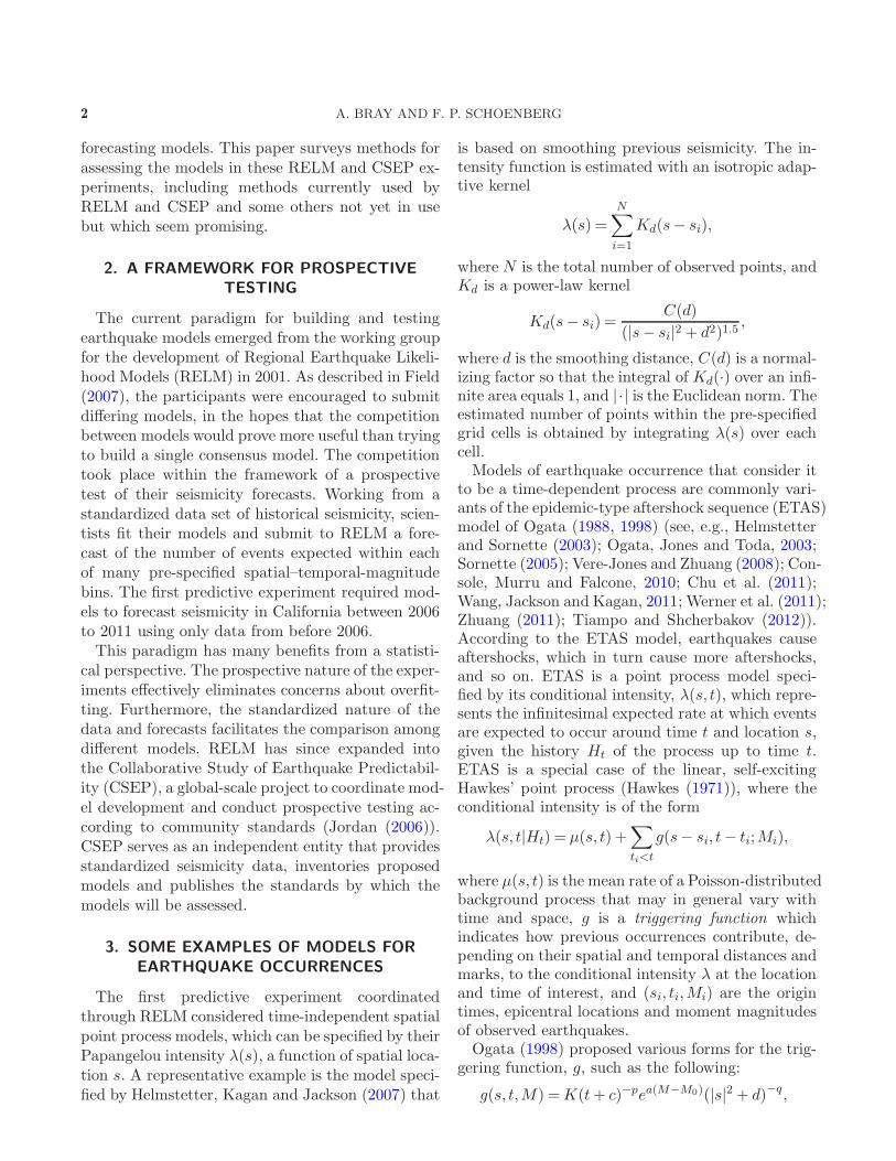
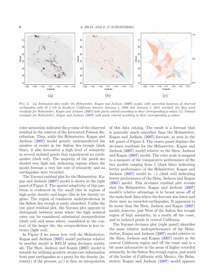
was submitted to RELM by Helmstetter, Kagan andJackson (2007) and is described in Section 3. Theleft panel of Figure 2 shows the estimated numberof earthquakes in every pixel in the greater Califor-nia region that were part of the prediction experi-ment. Pixels shaded very light gray have a forecastof near zero earthquakes, while pixels shaded blackforecast much greater seismicity. The tan circles arethe epicenters of the 232 earthquakes in the catalog,many of which are concentrated just South of theSalton Sea, near the border between California andMexico.The extent to which the observed seismicity is in

agreement with the forecast can be visualized in theraw pixel residual plot (center panel). The pixels arethose established by the RELM experiment. Pixelswhere the model predicted more events than wereobserved are shaded in red; pixels where there wasunderprediction are shown in blue. The degree of

8 A. BRAY AND F. P. SCHOENBERG

Fig. 2. (a) Estimated rates under the Helmstetter, Kagan and Jackson (2007) model, with epicentral locations of observedearthquakes with M ≥ 4.0 in Southern California between January 1, 2006 and January 1, 2011 overlaid. (b) Raw pixelresiduals for Helmstetter, Kagan and Jackson (2007) with pixels colored according to their corresponding p-values. (c) Voronolresiduals for Helmstetter, Kagan and Jackson (2007) with pixels colored according to their corresponding p-values.

color saturation indicates the p-value of the observedresidual in the context of the forecasted Poisson dis-tribution. Thus, while the Helmstetter, Kagan andJackson (2007) model greatly underpredicted thenumber of events in the Salton Sea trough (darkblue), it also forecasted a high level of seismicityin several isolated pixels that experienced no earth-quakes (dark red). The majority of the pixels areshaded very light red, indicating regions where themodel forecast a very low rate of seismicity and noearthquakes were recorded.The Voronoi residual plot for the Helmstetter, Ka-

gan and Jackson (2007) model is shown in the rightpanel of Figure 2. The spatial adaptivity of this par-tition is evidenced by the small tiles in regions ofhigh point density and larger tiles in low density re-gions. The region of consistent underprediction inthe Salton Sea trough is easily identified. Unlike theraw pixel residual plot, the Voronoi plot appears todistinguish between areas where the high isolatedrates can be considered substantial overprediction(dark red) and areas where, considered in the con-text of the larger tile, the overprediction is less ex-treme (light red).In Figure 3 we assess how well the Helmstetter,

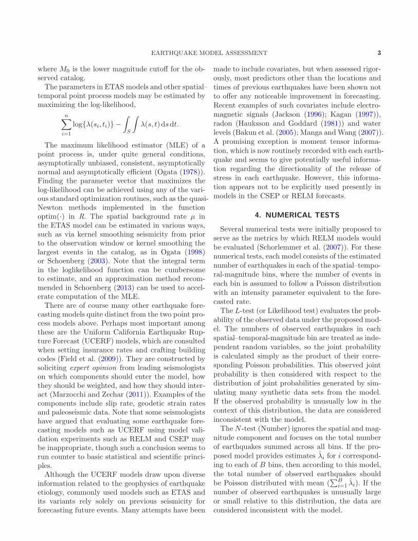
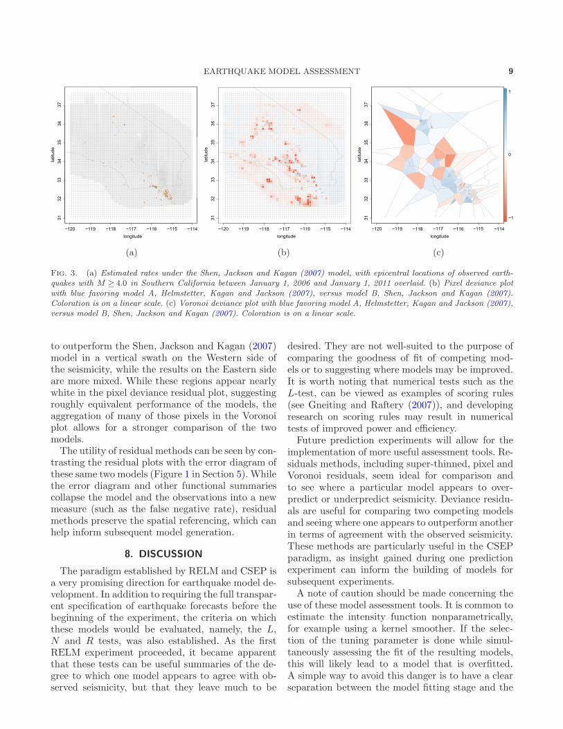
Kagan and Jackson (2007) model performs relativeto another model in RELM using deviance residu-als. The Shen, Jackson and Kagan (2007) model isnotable for utilizing geodetic strain-rate informationfrom past earthquakes as a proxy for the density (in-tensity) of the process. µ(·) is then an interpolation

of this data catalog. The result is a forecast thatis generally much smoother than the Helmstetter,Kagan and Jackson (2007) forecast, as seen in theleft panel of Figure 3. The center panel displays thedeviance residuals for the Helmstetter, Kagan andJackson (2007) model relative to the Shen, Jacksonand Kagan (2007) model. The color scale is mappedto a measure of the comparative performance of thetwo models ranging from 1 (dark blue) indicatingbetter performance of the Helmstetter, Kagan andJackson (2007) model to −1 (dark red) indicatingbetter performance of the Shen, Jackson and Kagan(2007) model. This deviance residual plot revealsthat the Helmstetter, Kagan and Jackson (2007)model’s relative advantage is in broad areas off ofthe main fault lines where the forecast was lower andthere were no recorded earthquakes. It appeared tofit worse than the Shen, Jackson and Kagan (2007)model, however, just West of the Salton Sea troughregion of high seismicity, in a swath off the coast,and in isolated pixels in central California.The Voronoi deviance plot (right panel) identifies

the same relative underperformance of the Helm-stetter, Kagan and Jackson (2007) model relative tothe Shen, Jackson and Kagan (2007) model in thecentral California region and off the coast and is abit more informative in the areas of higher recordedseismicity. In the Salton Sea trough region, just southof the border of California with Mexico, the Helm-stetter, Kagan and Jackson (2007) model appears

EARTHQUAKE MODEL ASSESSMENT 9

Fig. 3. (a) Estimated rates under the Shen, Jackson and Kagan (2007) model, with epicentral locations of observed earth-quakes with M ≥ 4.0 in Southern California between January 1, 2006 and January 1, 2011 overlaid. (b) Pixel deviance plotwith blue favoring model A, Helmstetter, Kagan and Jackson (2007), versus model B, Shen, Jackson and Kagan (2007).Coloration is on a linear scale. (c) Voronoi deviance plot with blue favoring model A, Helmstetter, Kagan and Jackson (2007),versus model B, Shen, Jackson and Kagan (2007). Coloration is on a linear scale.

to outperform the Shen, Jackson and Kagan (2007)model in a vertical swath on the Western side ofthe seismicity, while the results on the Eastern sideare more mixed. While these regions appear nearlywhite in the pixel deviance residual plot, suggestingroughly equivalent performance of the models, theaggregation of many of those pixels in the Voronoiplot allows for a stronger comparison of the twomodels.The utility of residual methods can be seen by con-

trasting the residual plots with the error diagram ofthese same two models (Figure 1 in Section 5). Whilethe error diagram and other functional summariescollapse the model and the observations into a newmeasure (such as the false negative rate), residualmethods preserve the spatial referencing, which canhelp inform subsequent model generation.

8. DISCUSSION

The paradigm established by RELM and CSEP isa very promising direction for earthquake model de-velopment. In addition to requiring the full transpar-ent specification of earthquake forecasts before thebeginning of the experiment, the criteria on whichthese models would be evaluated, namely, the L,N and R tests, was also established. As the firstRELM experiment proceeded, it became apparentthat these tests can be useful summaries of the de-gree to which one model appears to agree with ob-served seismicity, but that they leave much to be

desired. They are not well-suited to the purpose ofcomparing the goodness of fit of competing mod-els or to suggesting where models may be improved.It is worth noting that numerical tests such as theL-test, can be viewed as examples of scoring rules(see Gneiting and Raftery (2007)), and developingresearch on scoring rules may result in numericaltests of improved power and efficiency.Future prediction experiments will allow for the

implementation of more useful assessment tools. Re-siduals methods, including super-thinned, pixel andVoronoi residuals, seem ideal for comparison andto see where a particular model appears to over-predict or underpredict seismicity. Deviance residu-als are useful for comparing two competing modelsand seeing where one appears to outperform anotherin terms of agreement with the observed seismicity.These methods are particularly useful in the CSEPparadigm, as insight gained during one predictionexperiment can inform the building of models forsubsequent experiments.A note of caution should be made concerning the

use of these model assessment tools. It is common toestimate the intensity function nonparametrically,for example using a kernel smoother. If the selec-tion of the tuning parameter is done while simul-taneously assessing the fit of the resulting models,this will likely lead to a model that is overfitted.A simple way to avoid this danger is to have a clearseparation between the model fitting stage and the

10 A. BRAY AND F. P. SCHOENBERG

model assessment stage, as occurs when models aredeveloped for prospective experiments.Although the best fitting models for forecasting

earthquake occurrences involve clustering and arethus highly non-Poissonian, it is unclear whetherthe Poisson assumption implicit in the evaluation

of these models in CSEP or RELM has anythingmore than a negligible impact on the results. Sincethe quadrats used in these forecast evaluations arerather large, the dependence between the numbers ofevents occurring in adjacent pixels may be slight af-ter accounting for inhomogeneity. Further, a depar-ture from the Poisson distribution for the number ofevents occurring within a given cell would typicallyhave similar impacts on competing forecast modelsand thus have little noticeable effect when it comesto evaluation of the relative performance of com-peting models. Nonetheless, further study is neededto clarify the importance of this assumption in theCSEP model evaluation framework. An alternativeapproach to the Poisson model would be to requirethat modelers provide not only the expected num-ber of earthquakes within each bin, but also the jointprobability distribution of counts within the bins.Although this paper has focused on assessment

tools for earthquake models, there is a wide range ofpoint process models to which these methods can beapplied. Super-thinned residuals and theK-functionhave been useful in assessing models of invasivespecies (Balderama et al. (2012)). Other recent ex-amples, such as the use of functional summaries in astudy of infectious disease, can be found in Gelfandet al. (2010).

ACKNOWLEDGMENTS

We thank the Editor, Associate Editor and refer-ees for very thoughtful remarks which substantiallyimproved this paper.

REFERENCES

Adelfio, G. and Schoenberg, F. P. (2009). Point processdiagnostics based on weighted second-order statistics andtheir asymptotic properties. Ann. Inst. Statist. Math. 61

929–948. MR2556772Baddeley, A. J., Møller, J. and Waagepetersen, R.

(2000). Non- and semi-parametric estimation of interactionin inhomogeneous point patterns. Stat. Neerl. 54 329–350.MR1804002

Baddeley, A., Møller, J. and Pakes, A. G. (2008). Prop-erties of residuals for spatial point processes. Ann. Inst.Statist. Math. 60 627–649. MR2434415

Baddeley, A., Turner, R., Møller, J. and Hazelton, M.

(2005). Residual analysis for spatial point processes. J. R.Stat. Soc. Ser. B Stat. Methodol. 67 617–666. MR2210685

Bakun, W. H., Aagaard, B., Dost, B.,Ellsworth, W. L., Hardebeck, J. L., Har-

ris, R. A., Ji, C., Johnston, M. J. S., Langbein, J.,Lienkaemper, J. J., Michael, A. J., Murray, J. R.,Nadeau, R. M., Reasenberg, P. A., Reichle, M. S.,Roeloffs, E. A., Shakal, A., Simpson, R. W. andWaldhauser, F. (2005). Implications for prediction andhazard assessment from the 2004 Parkfield earthquake.Nature 437 969–974.

Balderama, E., Schoenberg, F. P., Murray, E. andRundel, P. W. (2012). Application of branching modelsin the study of invasive species. J. Amer. Statist. Assoc.107 467–476. MR2980058

Bolt, B. (2003). Earthquakes, 5th ed. Freeman, New York.Bray, A., Wong, K., Barr, C. and Schoenberg, F. P.

(2014). Residuals for spatial point processes based onVoronoi tessellations. Ann. Appl. Stat. To appear.

Bremaud, P. (1981). Point Processes and Queues: Martin-gale Dynamics. Springer, New York. MR0636252

Chu, A., Schoenberg, F. P., Bird, P., Jackson, D. D.

and Kagan, Y. Y. (2011). Comparison of ETAS param-eter estimates across different global tectonic zones. Bull.Seismol. Soc. Amer. 101 2323–2339.

Clements, R. A., Schoenberg, F. P. and Schorlem-

mer, D. (2011). Residual analysis methods for space–time point processes with applications to earthquake fore-cast models in California. Ann. Appl. Stat. 5 2549–2571.MR2907126

Clements, R. A., Schoenberg, F. P. and Veen, A. (2012).Evaluation of space-time point process models using super-thinning. Environmetrics 23 606–616. MR3020078

Console, R., Murru, M. and Falcone, G. (2010). Proba-bility gains of an epidemic-type aftershock sequence modelin retrospective forecasting of M ≥ 5 earthquakes in Italy.J. Seismology 14 9–26.

Field, E. H. (2007). Overview of the working group for thedevelopment of regional earthquake models (RELM). Seis-mological Research Letters 78 7–16.

Field, E. H., Dawson, T. E., Felzer, K. R.,Frankel, A. D., Gupta, V., Jordan, T. H., Par-

sons, T., Petersen, M. D., Stein, R. S., Weldon, R. J.

and Wills, C. J. (2009). Uniform California EarthquakeRupture Forecast, Version 2 (UCERF 2). Bull. Seismol.Soc. Amer. 99 2053–2107.

Gelfand, A., Diggle, P., Guttorp, P. and Fuentes, M.,eds. (2010). Handbook of Spatial Statistics. CRC Press,Boca Raton, FL. MR2761512

Geller, R. J., Jackson, D. D., Kagan, Y. Y. and Mula-

rgia, F. (1997). Earthquakes cannot be predicted. Science275 1616–1617.

Gneiting, T. and Raftery, A. E. (2007). Strictly properscoring rules, prediction, and estimation. J. Amer. Statist.Assoc. 102 359–378. MR2345548

Hauksson, E. and Goddard, J. G. (1981). Radon earth-quake precursor studies in Iceland. J. Geophys. Res. 86

7037–7054.

EARTHQUAKE MODEL ASSESSMENT 11

Hawkes, A. G. (1971). Point spectra of some mutually excit-ing point processes. J. R. Stat. Soc. Ser. B Stat. Methodol.33 438–443. MR0358976

Helmstetter, A., Kagan, Y. Y. and Jackson, D. D.

(2007). High-resolution time-independent grid-based fore-cast M ≥ 5 earthquakes in California. Seismological Re-search Letters 78 78–86.

Helmstetter, A. and Sornette, D. (2003). Predictabilityin the Epidemic-Type Aftershock Sequence model of in-teracting triggered seismicity. J. Geophys. Res. 108 2482–2499.

Hough, S. (2010). Predicting the Unpredictable: The Tumul-tuous Science of Earthquake Prediction. Princeton Univ.Press, Princeton, NJ.

Jackson, D. D. (1996). Earthquake prediction evaluationstandards applied to the VAN method. Geophys. Res. Lett.23 1363–1366.

Jordan, T. H. (2006). Earthquake predictability, brick bybrick. Seismological Research Letters 77 3–6.

Jordan, T. H. and Jones, L. M. (2010). Operational earth-quake forecasting: Some thoughts on why and how. Seis-mological Research Letters 81 571–574.

Kagan, Y. Y. (1997). Are earthquakes predictable? Geophys.J. Int. 131 505–525.

Kagan, Y. Y. (2009). Testing long-term earthquake fore-casts: Likelihood methods and error diagrams. Geophys.J. Int. 177 532–542.

Keilis-Borok, V. and Kossobokov, V. G. (1990). Premon-itory activation of earthquake flow: Algorithm M8. Physicsof the Earth and Planetary Interiors 6 73–83.

Lewis, P. A. W. and Shedler, G. S. (1979). Simulationof nonhomogeneous Poisson processes by thinning. NavalRes. Logist. Quart. 26 403–413. MR0546120

Manga, M. and Wang, C. Y. (2007). Earthquake hydrology.In Treatise on Geophysics (G. Schubert, ed.) 4 293–320.Elsevier, Amsterdam.

Marzocchi, W. and Zechar, J. D. (2011). Earthquake fore-casting and earthquake prediction: Different approaches forobtaining the best model. Seismological Research Letters 82442–448.

Merzbach, E. and Nualart, D. (1986). A characterizationof the spatial Poisson process and changing time. Ann.Probab. 14 1380–1390. MR0866358

Meyer, P. A. (1971). Demonstration simplifiee d’untheoreme de Knight. In Seminaire de Probabilites, V (Univ.Strasbourg, Annee Universitaire 1969–1970) Lecture Notesin Math. 191 191–195. Springer, Berlin. MR0380972

Molchan, G. M. (1991). Structure of optimal strategies inearthquake prediction. Tectonophysics 193 267–276.

Molchan, G. (2010). Space-time earthquake prediction: Theerror diagrams. Pure and Applied Geophysics 167 907–917.

Nair, M. G. (1990). Random space change for multi-parameter point processes. Ann. Probab. 18 1222–1231.MR1062066

Ogata, Y. (1978). The asymptotic behaviour of maximumlikelihood estimators for stationary point processes. Ann.Inst. Statist. Math. 30 243–261. MR0514494

Ogata, Y. (1981). On Lewis’ simulation method for pointprocesses. IEEE Trans. Inform. Theory IT-27 23–31.

Ogata, Y. (1988). Statistical models for earthquake occur-rences and residual analysis for point processes. J. Amer.Statist. Assoc. 83 9–27.

Ogata, Y. (1998). Space–time point process models for earth-quake occurrences. Ann. Inst. Statist. Math. 50 379–402.

Ogata, Y., Jones, L. M. and Toda, S. (2003). When andwhere the aftershock activity was depressed: Contrast-ing decay patterns of the proximate large earthquakes insouthern California. Journal of Geophysical Research 108

2318.Okabe, A., Boots, B., Sugihara, K. and Chiu, S. N.

(2000). Spatial Tessellations: Concepts and Applications ofVoronoi Diagrams, 2nd ed. Wiley, Chichester. MR1770006

Rhoades, D. A., Schorlemmer, D., Gersten-

berger, M. C., Christophersen, A., Zechar, J. D.

and Imoto, M. (2011). Efficient testing of earthquakeforecasting models. Acta Geophysica 59 728–747.

Ripley, B. D. (1976). The second-order analysis of stationarypoint processes. J. Appl. Probab. 13 255–266. MR0402918

Schoenberg, F. (1999). Transforming spatial point processesinto Poisson processes. Stochastic Process. Appl. 81 155–164. MR1694573

Schoenberg, F. P. (2003). Multidimensional residual anal-ysis of point process models for earthquake occurrences. J.Amer. Statist. Assoc. 98 789–795. MR2055487

Schoenberg, F. P. (2013). Facilitated estimation of ETAS.Bulletin of the Seismological Society of America 103 1–7.

Schorlemmer, D., Gerstenberger, M. C., Wiemer, S.,Jackson, D. D. and Rhoades, D. A. (2007). Earthquakelikelihood model testing. Seismological Research Letters 7817–27.

Shen, Z. K., Jackson, D. D. and Kagan, Y. Y. (2007).Implications of geodetic strain rate for future earthquakes,with a five-year forecast of M5 earthquakes in southernCalifornia. Seismological Research Letters 78 116–120.

Sornette, D. (2005). Apparent clustering and apparentbackground earthquakes biased by undetected seismicity.J. Geophys. Res. 110 B09303.

Swets, J. A. (1973). The relative operating characteristic inpsychology. Science 182 990–1000.

Tiampo, K. R. and Shcherbakov, R. (2012). Seismicity-based earthquake forecasting techniques: Ten years ofprogress. Tectonophysics 522 89–121.

Veen, A. and Schoenberg, F. P. (2006). Assessing spatialpoint process models using weighted K-functions: Analysisof California earthquakes. In Case Studies in Spatial PointProcess Modeling (A. Baddeley, P. Gregori, J. Mateu,R. Stoica and D. Stoyan, eds.). Lecture Notes in Statist.185 293–306. Springer, New York. MR2232135

Vere-Jones, D. and Schoenberg, F. P. (2004). Rescalingmarked point processes. Aust. N. Z. J. Stat. 46 133–143.MR2055791

Vere-Jones, D. and Zhuang, J. (2008). On the distributionof the largest event in the critical ETAS model. Phys. Rev.E (3) 78 047102.

Wang, Q., Jackson, D. D. and Kagan, Y. Y. (2011). Cal-ifornia earthquake forecasts based on smoothed seismic-ity: Model choices. Bull. Seismol. Soc. Amer. 101 1422–1430.

12 A. BRAY AND F. P. SCHOENBERG

Werner, M. J., Helmstetter, A., Jackson, D. D. andKagan, Y. Y. (2011). High-Resolution Long-Term andShort-Term Earthquake Forecasts for California. Bull.Seismol. Soc. Amer. 101 1630–1648.

Zaliapin, I. and Molchan, G. (2004). Tossing the earth:How to reliably test earthquake prediction methods. Eos.Trans. AGU 85 47. S23A–0302.

Zechar, J. D., Gerstenberger, M. C. andRhoades, D. A. (2010). Likelihood-based tests forevaluating space–rate-magnitude earthquake forecasts.Bull. Seismol. Soc. Amer. 100 1184–1195.

Zechar, J. D. and Jordan, T. H. (2008). Testing alarm-based earthquake predictions. Geophys. J. Int. 172 715–724.

Zechar, J. D., Schorlemmer, D., Werner, M. J., Ger-

stenberger, M. C., Rhoades, D. A. and Jordan, T. H.

(2013). Regional earthquake likelihood models I: First-order results. Unpublished manuscript.

Zhuang, J. (2011). Next-day earthquake forecasts for theJapan region generated by the ETAS model. Earth PlanetsSpace 63 207–216.