assessment of proposed approaches for bathymetry
TRANSCRIPT

ORIGINAL PAPER
Assessment of proposed approaches for bathymetry calculationsusing multispectral satellite images in shallow coastal/lake areas:a comparison of five models
Hassan Mohamed1& AbdelazimNegm1
& Mahmoud Salah2& Kazuo Nadaoka3 &
Mohamed Zahran2
Received: 1 December 2015 /Accepted: 20 December 2016 /Published online: 18 January 2017# Saudi Society for Geosciences 2017
Abstract Bathymetric information for shallow coastal/lakeareas is essential for hydrological engineering applicationssuch as sedimentary processes and coastal studies. Remotelysensed imagery is considered a time-effective, low-cost, andwide-coverage solution for bathymetric measurements. Thisstudy assesses the performance of three proposed empiricalmodels for bathymetry calculations in three different areas:Alexandria port, Egypt, as an example of a low-turbidity deepwater area with silt-sand bottom cover and a depth range of10.5 m; the Lake Nubia entrance zone, Sudan, which is ahighly turbid, unstable, clay bottom area with water depthsto 6 m; and Shiraho, Ishigaki Island, Japan, a coral reef areawith varied depths ranging up to 14 m. The proposed modelsare the ensemble regression tree-fitting algorithm using bag-ging (BAG), ensemble regression tree-fitting algorithm of
least squares boosting (LSB), and support vector regressionalgorithm (SVR). Data from Landsat 8 and Spot 6 satelliteimages were used to assess the performance of the proposedmodels. The three models were used to obtain bathymetricmaps using the reflectance of green, red, blue/red, andgreen/red band ratios. The results were compared with corre-sponding results yielded by two conventional empiricalmethods, the neural network (NN) and the Lyzenga general-ised linear model (GLM). Compared with echosounder data,BAG, LSB, and SVR results demonstrate higher accuracyranges from 0.04 to 0.35 m more than Lyzenga GLM. TheBAG algorithm, producing the most accurate results, provedto be the preferable algorithm for bathymetry calculation.
Keywords Bagging . Boosting . Bathymetry . Landsat 8 .
Spot 6 . Support vector regression
Introduction
Coastal/lake area bathymetry is considered to be of fundamen-tal importance for many purposes and applications, such ascoastal engineering sciences, sustainable management, andspatial planning of lakes (Leu and Chang 2005; Gao 2009).These areas have changeable sediment movements due to tidalcurrents, wave propagation, and intensive human activities(Ceyhun and Yalçın 2010). As a result, rapid and accuratemonitoring measurements of these regions, especially waterbottom levels, should be developed (Pacheco et al. 2015).
Currently, there are two methods for water depth detection:single–multibeam echosounders and Lidar. The multibeamechosounder is the most conventional method for bathymetricapplications, especially for very deep waters with depths up to500 m. High accuracy and full-bottom coverage are consideredto be the main advantages of the multibeam echosounder. In
* Hassan [email protected]
* Mahmoud [email protected]
Kazuo [email protected]
Mohamed [email protected]
1 Department of Environmental Engineering, Egypt-Japan Universityof Science and Technology E-JUST, New Borg El-Arab,Alexandria, Egypt
2 Department of Surveying Engineering, Faculty of Engineering atShoubra, Benha University, Benha, Egypt
3 Department of Transdisciplinary Science and Engineering, TokyoInstitute of Technology, Tokyo, Japan
Arab J Geosci (2017) 10: 42DOI 10.1007/s12517-016-2803-1

addition, the single-beam echosounder represents a feasible al-ternative for producing sea-bottom maps with acceptable verti-cal accuracy at a lower cost than that of the multibeamechosounder (Sánchez-Carnero et al. 2012). However, both ofthese methods are expensive, time-consuming, and require in-tensive labor, especially in shallow areas where coral reefs,rocks, and general shallowness are an obstacle to the navigationof survey boats. Finally, Lidar technology has been developedfor bathymetric applications through the past several decades.Despite their high level of depth accuracy and suitability toshallow coastal areas, these systems are extremely expensiveand have comparatively low coverage (Chust et al. 2010).
Optical remote sensing represents a low-cost, wide-cover-age, and time-effective alternative to single–multibeamechosounders and Lidar for coastal bathymetry monitoringapplications (Sánchez-Carnero et al. 2014). Lyzenga (1985)introduced the log-linear empirical approach using single im-agery band for detecting water depths from satellite images.His theory was dependent on removing all other reflectedvalues influencing water bottom signals. Recently, a log-linear correlation between multiband and water depth valueswas proposed by Lyzenga et al. (2006). Lyzenga et al.’s (2006)approach was applied subsequently by other researchers usingdifferent satellite images: Quickbird (Lyons et al. 2011),Worldview 2 (Doxani et al. 2012), Spot 4 (Sánchez-Carneroet al. 2014), and Landsat 8 images (Pacheco et al. 2015).Another empirical approach depending on band ratios, inwhich the difference in attenuation for different bands can beused for bathymetry detection, was developed by Stumpf et al.(2003). In the following years, this approach was developedfurther by other researchers such as Su et al. (2008) andBramante et al. (2013).
Both of these empirical approaches which considered themost simple and widely used water depth derivation methods(Vahtmäe and Kutser 2016) have limitations. The first ap-proach supposes that the entire bottom surface is homogenousand that the water column is similar in the entire coveragearea. The second approach overcomes this demerit, but ithas no physical foundation and its parameters are calculatedthrough a trial process (Gholamalifard et al. 2013).
In the last decades, a novel alternative approach was pro-posed for detecting bathymetry using the neural network (NN)algorithm by Ceyhun and Yalçın (2010). This algorithm per-forms a non-linear relation between all spectral bands andwater depth values, overcoming the limitations of the regres-sive models. Recently, other researchers have applied thesame algorithm to various water depths, with various satelliteimages, and argued the outperformance to conventionalLyzenga and Stumpf approaches. Examples include Landsatimages (Gholamalifard et al. 2013), IRS P6-LISS III images(Moses et al. 2013), and Quickbird images (Corucci 2011),using the neuro-fuzzy approach. This method has many dis-advantages such as its complexity, black box nature,
sensitivity to any small changes in data values resulting inhigh variance in output results, and vulnerability to theoverfitting process. Moreover, it requires a lot of data or spec-tral bands to detect bathymetry.
On the other hand, comparative analytical methods usingspectral libraries (look-up tables) in interpretation of remotesensing data have gained popularity in the mapping of waterdepths (Mobley et al. 2005; Lesser and Mobley 2007; Brandoet al. 2009). These approaches need the spectral data about thebottom reflectance, suspended and dissolved matters, and ap-plied with hyperspectral images (Vahtmäe and Kutser 2016).However, these approaches have three major limitations. First,the hyperspectral images are not available for enormous zonesand have coarse spatial resolution. Also, the alternative air-borne systems are expensive especially for wide coverage.Second, the processing of the hyperspectral imagery is com-putationally hard. Finally, they are relatively complexmethods. This makes the empirical models with multispectralimagery a valuable alternative (Bramante et al. 2013).
The objective of this research is proposing three simpleempirical approaches for bathymetry detection in shallowcoastal/lake areas and attempts to overcome the drawbacksof the NN and Lyzenga GLM methods. These approachesare the ensemble regression tree-fitting algorithm using bag-ging (BAG), the ensemble regression tree-fitting algorithm ofleast squares boosting (LSB), and the support vector regres-sion algorithm (SVR). The three algorithms are more stable,simpler, and more invulnerable to overfitting than NN; aremuch simpler than analytical approaches; and are less affectedby other environmental factors than the Lyzenga GLM. Theproposed methodologies were applied using Spot 6 andLandsat 8 images as example of high and low spatial resolu-tions over various study areas. The reflectance of green, red,blue/red, and green/red band ratios were used to obtain bathy-metric maps as they demonstrate high correlation with waterdepths. To support the robustness of these approaches, threestudy areas were selected to provide diverse bottom sampleswith different levels of turbidity. The results achieved werethen evaluated and compared with echosounder bathymetricdata over three different study areas.
Study areas and available data
The first study area was Alexandria port, Egypt (see Fig. 1a).It is a fairly deep, low-turbidity, calm water area, due to itscoastal barriers and has a depth range of 10.5m. Almost all theharbor bottom surface cover is silt-sand. The second studyarea was the entrance zone of Lake Nasser/Nubia, which islocated in the Sudanese part of Lake Nubia (see Fig. 1b). It is afairly irregular, shallow, highly turbid water area with depthsup to 6 m and high rates of sediment changes and annual floodchanges. The lake has a clayey bottom surface.
42 Page 2 of 17 Arab J Geosci (2017) 10: 42

The third study area was Shiraho, a subtropical territory,which is located in the southeastern part of Ishigaki Island,Japan (see Fig. 2). It is an irregularly shallow, low-turbid waterarea with depths up to 14 m. Shiraho is a heterogeneous areawith a rich marine biodiversity that includes various ecosys-tems such as mangroves, seagrasses, and coral reefs.
Imagery data
Freely available Landsat 8 satellite images were used for de-tecting the bathymetry of the first and the third study areaswith a spatial resolution of 30 m. Spot 6 image with a spatialresolution of 1.5 m was used for the second study area. Therequired parameters for radiometric image corrections wereavailable in the images’ metadata files. The first Landsat 8image was acquired during calm weather conditions on 3August 2014, and the second Landsat 8 image was collectedduring windy conditions on 5 June 2013. The Spot 6 imagewas acquired during calm weather conditions on 12 January2014. These images were selected so as to be synchronizedwith the echosounder field collection times for each studyarea.
Echosounder data
The reference water depths of the first study areas used forcalibrating the algorithms were acquired by a NaviSoundHydrographic Systems model 210 echosounder instrumentwith an attached Trimble 2000 GPS. The maximum depthrange of the echosounder was 400 m, and its vertical accuracy
Fig. 1 a The first study area of Alexandria port coastal area, Egypt. b The second study area of Nubia Lake entrance zone, Sudan
Fig. 2 The third study area of Shiraho, Ishigaki Island, Japan
Arab J Geosci (2017) 10: 42 Page 3 of 17 42

was 1 cm at 210 kHz (see Fig. 3). The second study area’swater depths were acquired by an Odom HydrographicSystems Echotrac model DF 3200 MKII echosounder instru-ment with built-in DGPS. The depth range of the echosounderwas from 0.2 to 200 m and its vertical accuracy was0.01 m ± 0.1% of depth (see Fig. 4). Finally, the referencewater depths of the third study area were acquired by asingle-beam Lowrance LCX-15MT dual frequency (50/200 kHz) transducer and 12-channel GPS antenna. The hori-zontal and vertical accuracies were ±1 and ±0.03 m, respec-tively (Collin et al. 2014) (see Fig. 5).
About 2500 field points were collected for the first studyarea, 12,500 for the second study area, and 14,500 for the thirdstudy area. All the water depths were referenced to mean sealevel (MSL). These points were used for calibration and eval-uation of all the bathymetric models.
Methodology
To determine bathymetric information from the satellite im-ages, pixel values were first converted to radiometrically cor-rect spectral radiance values (Todd and Chris 2010). The datarequired for this conversion were available in the images’metadata files (MTL files). Then, two essential successivecorrections were applied to the radiance images: the sun glintcorrection and the atmospheric correction (Doxani et al.2012). The sequence of implementation of these two correc-tions is optional (Kay et al. 2009). Second, the input values fortraining the supervised regression algorithms were extractedfrom the corrected reflectance images at the correspondinglocations of the echosounder field points. Four inputs are usedfor training each approach: the values of red, green, blue/red,and green/red bands logarithms and the outputs were the water
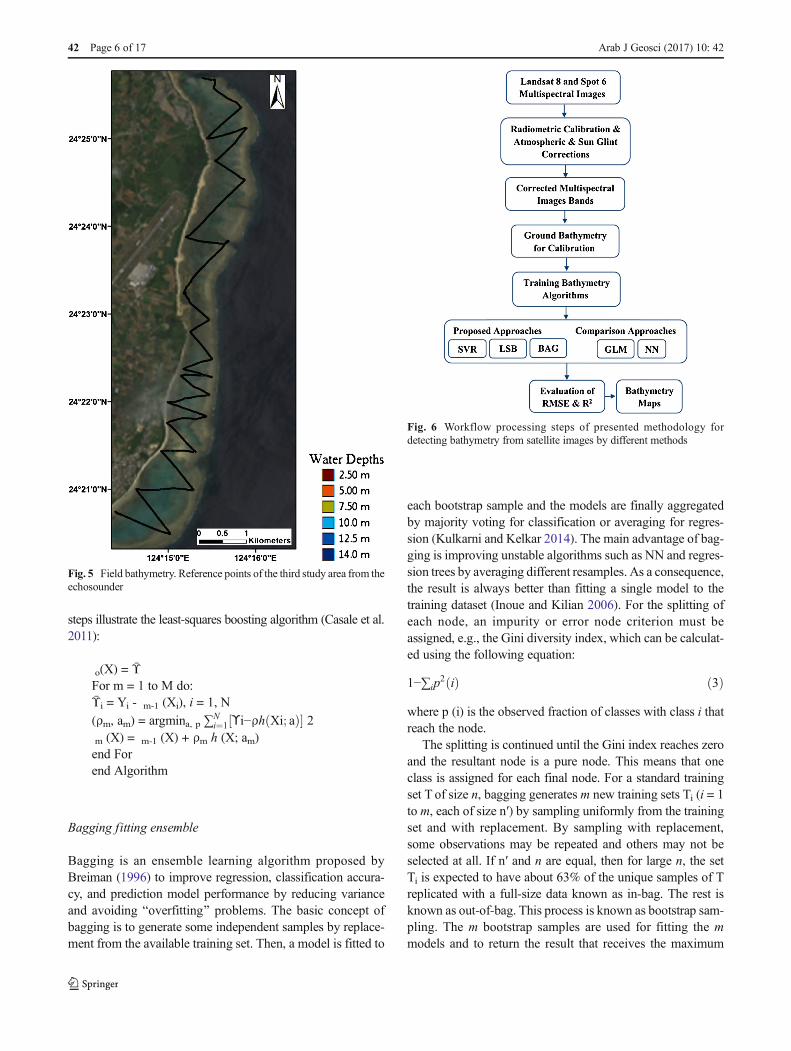
depths. For all study areas, the number of the sounding pointswas randomly divided to independent 75% training points and25% testing points. For instance, for the Alex port study area,the sounding points were divided to 1875 points for trainingand 625 points for testing. Finally, the outputs from all algo-rithms were evaluated using the same independent testingpoints. The comparison depended on the RMSE and R2 valuesresulting from the difference between the extracted bathymet-ric values and testing points of all approaches. Figure 6 sum-marises the workflow of these steps.
The following subsections describe the imagery datapreprocessing.
Imagery data preprocessing
Spectral top of atmosphere radiance
The spectral top of atmosphere radiance of each pixelwas computed from the imagery pixel digital number(DN) values using the following equation (Landsat-82013):
Lλ ¼ Ml*DNþ Al ð1Þ
where Lλ = top of atmosphere spectral radiance, DN = digitalnumber recorded by the sensor, Ml = band-specific multipli-cative rescaling factor for radiances, and Al = band-specificadditive rescaling factor for radiances.
The Ml and Al values were available in the images’ meta-data files (MTL files).
Atmospheric correction
Atmospheric correction was applied to all images using theFast Line-of-Sight Atmospheric Analysis of Hypercubes
Fig. 3 Field bathymetry.Reference points of the first studyarea from the echosounder
42 Page 4 of 17 Arab J Geosci (2017) 10: 42

(FLAASH™) tool in the Envi 5.3 program. FLAASHperforms radiative transfer-based models based onMODTRAN4 code (Berk et al. 1998) and has look-up tablesfor different types of atmosphere. Different types of aerosolsare supported in the FLAASH tool, which defines theparticle properties as scattering, absorption, and wave-length path radiance performance. The calculated radi-ance images were used as input for FLAASH tool. Forall study areas, the maritime types were selected as aero-sol model type, tropical as atmospheric model for hotareas, and two blue and infrared bands over water wereselected as aerosol retrieval (Su et al. 2008). Finally,atmospherically corrected reflectance images were pro-duced as the result.
Sun glint correction
The sun glint correction was applied to the atmosphericallycorrected reflectance images using the relation between thebands used for bathymetry and the near-infrared band(Hedley et al. 2005; Sánchez-Carnero et al. 2014). Thedeglinted pixel value can be calculated using Eq. 2:
Ri0 ¼ Ri*bi RNIR−MinNIRð Þ ð2Þ
where R i ′ = deg l in ted p ixe l re f l ec tance va lue ,Ri = atmospherically corrected reflectance value, bi = regres-sion line slope, RNIR = corresponding pixel value in NIRband, and MinNIR = min NIR value existing in the sample.
Proposed approaches for bathymetry estimation
Least squares boosting fitting ensemble
Boosting is considered to be one of themost powerful learningensemble algorithms to be proposed recently. It was originallydesigned for classification, but it was found that it could alsobe used for regression problems (Hastie et al. 2009). The basicconcept of boosting is to develop multiple models in sequenceby assigning higher weights as boosting for those trainingcases or learners that are difficult to be fitted in regressionproblems (Quinlan 2006). In this approach, learners learn se-quentially, with early learners fitting simple models of data,and then the data are analyzed for errors. These errors identifyproblems of particular samples of data that are difficult to fit.Later models focus primarily on these samples by giving themhigher weights and trying to predict them correctly. Finally, allmodels are given weights, and the set is converted to someoverall predictors.
Thus, boosting is a method of converting a sequence ofweak learners into strong predictors or a way of increasingthe complexity of the primary model. Initial learners oftenare very simple, but the weighted combination can developstronger and more complex learners (Ihler 2012).
The least-squares algorithm can be used to minimize anydifferentiable loss L(y, F) in conjunction with forward stagewiseadditive modeling in order to fit the generic function h (X, a) tothe pseudo-responses (Ῡ = −gm (Xi)) for i = 1… N. In least-squares regression, the loss of function is L(Y, ) = (Y − ) 2/2 andthe pseudo-response is Ῡi = Y I − m − 1 (Xi). The following
Fig. 4 In-situ bathymetry.Reference points of the secondstudy area from the echosounder
Arab J Geosci (2017) 10: 42 Page 5 of 17 42
steps illustrate the least-squares boosting algorithm (Casale et al.2011):
o(X) = ῩFor m = 1 to M do:Ῡi = Yi - m-1 (Xi), i = 1, N
(ρm, am) = argmina, p ∑Ni¼1 ϒi−ρh Xi; að Þ½ � 2
m (X) = m-1 (X) + ρm h (X; am)end Forend Algorithm
Bagging fitting ensemble
Bagging is an ensemble learning algorithm proposed byBreiman (1996) to improve regression, classification accura-cy, and prediction model performance by reducing varianceand avoiding Boverfitting^ problems. The basic concept ofbagging is to generate some independent samples by replace-ment from the available training set. Then, a model is fitted to
each bootstrap sample and the models are finally aggregatedby majority voting for classification or averaging for regres-sion (Kulkarni and Kelkar 2014). The main advantage of bag-ging is improving unstable algorithms such as NN and regres-sion trees by averaging different resamples. As a consequence,the result is always better than fitting a single model to thetraining dataset (Inoue and Kilian 2006). For the splitting ofeach node, an impurity or error node criterion must beassigned, e.g., the Gini diversity index, which can be calculat-ed using the following equation:
1−∑ip2 ið Þ ð3Þ
where p (i) is the observed fraction of classes with class i thatreach the node.
The splitting is continued until the Gini index reaches zeroand the resultant node is a pure node. This means that oneclass is assigned for each final node. For a standard trainingset T of size n, bagging generates m new training sets Ti (i = 1to m, each of size n′) by sampling uniformly from the trainingset and with replacement. By sampling with replacement,some observations may be repeated and others may not beselected at all. If n′ and n are equal, then for large n, the setTi is expected to have about 63% of the unique samples of Treplicated with a full-size data known as in-bag. The rest isknown as out-of-bag. This process is known as bootstrap sam-pling. The m bootstrap samples are used for fitting the mmodels and to return the result that receives the maximum
Fig. 5 Field bathymetry. Reference points of the third study area from theechosounder
Fig. 6 Workflow processing steps of presented methodology fordetecting bathymetry from satellite images by different methods
42 Page 6 of 17 Arab J Geosci (2017) 10: 42

number of votes H (x) (Ghimire et al. 2012). The followingsteps elucidate the bagging algorithm (Galar et al. 2012):
For m = 1 to M doTm = Random sample replacement (n, T)hm = L (Tm)end for
H (x) = sign ( ∑M
m¼1hm xð Þ ) where hm∊ [−1, 1] are the
induced classifiersEnd algorithm
Support vector regression
Vapnik et al. (1964) proposed support vector machines(SVMs) for solving classification problems and statisticallearning applications. As the method has shown high perfor-mance and has resulted in high accuracies, it has been extend-ed successfully to regression problems. To discuss any regres-sion problem, suppose that we have a training dataset ofD = {yi, ti and i = 1, 2, 3…n}, with input vectors yi and targetvectors ti. The main regression problem is to find a fittingfunction f (y) that approximates the relation between the inputand target points. In addition, the output t is interpreted for anynew input point y. This regression fitting function has a loss offunction describing the difference between the predictedvalues and the actual target values (Smola and Schölkopf2004). The support vector regression finds the most possibleflat and deviated insensitive loss of function ε from the realtargets (Vapnik 2000). In other words, errors are allowed if it isless than the predefined ε that controls the tolerance; other-wise, they are not. Suppose that we have a linear problemwiththe following equation
F xð Þ ¼ w*yþ b ð4Þ
where w ∍ y and b ∍ R, both w and y are the dot product of wand y, and b is the bias.
Flatness in regression problems means searching for a smallvalue for w, or in other words, minimixing the norm Euclidianspace ‖w‖2. Thus, the regression can be stated as a convexoptimisation problem as follows (Smola and Schölkopf 2004):
Minimize 12 wk k2
Subject to
ti− w:yð Þ þ b ≤εw:yð Þ−tiþ b ≤ε
�ð5Þ
However, this formula assumes that all points are approxi-mated within the allowable precision ε, which is not a feasibleassumption in all cases, and some exceeding errors need to beallowed. Cortes and Vapnik (1995) used a soft margin loss
function to present slack variables ζi to overcome this problem,and the support vector regression solves this problem as follows:
Minimize 12 wk k2 þ C∑n
i¼1 ζiþζi*� �
Subject to
ti− w⋅yð Þ þ b≤εþ ζiw⋅yð Þ−tiþ b≤εþ ζi*
ζi; ζ ix
8<: ð6Þ
where C represents the compromise between the flatness andthe tolerated deviation larger than ε. The points outside ε arecalled support vectors.
It was found that solving this optimzation problem is easierin its dual formulation and by extending the SVM to non-linear functions. As a result, a standard dualisation methodusing Lagrange multipliers can be applied to solve the SVRoptimization problem. A Lagrange function can be construct-ed from the objective function by defining a dual set of vari-ables. The dual optimisation problem can be written as fol-lows (Farag and Mohamed 2004):
Maximize
−1
2∑l
i; j¼1αi−αi
x� �
αj−α jx
� �yi; yjð Þ
−ε ∑l
i¼1αiþ αi
x� �
þ ∑l
i¼1xi αi−αi
x� �
8>><>>:
Subject to
∑li¼1 αi−α i
x� �¼ 0
αi;α ix� �
∈ 0;C½ �
8<: ð7Þ
where αi and αi are Lagrange multipliers.As a result, w and the expansion of F(x) can be calculated
as follows:
W ¼ ∑ni¼1 αi−α i
x� �xi and F xð Þ
¼ ∑li¼1 αi−α i
x� �yi; yjð Þ þ b ð8Þ
These equations infer thatw can be calculated from a linearcombination of the training sets of yi.
The bias term b is calculated using the Karush KuhnTucker (KKT) conditions (Karush 1939; Kuhn and Tucker1951) as follows:
b ¼ xi− w; yð Þ−ε for αi0 0;Cð Þ ð9Þ
The non-linearity of the support vector algorithm can beperformed by preprocessing the training sets yi with a mapФ:y → into some feature space . Figure 7 illustrates the con-version from the decision boundary into a hyperplane aftermapping to a feature space.
Arab J Geosci (2017) 10: 42 Page 7 of 17 42

For a feasible solution, a kernel k (y, y’) can be used, andthe support vector regression algorithm can be rewritten asfollows (Farag and Mohamed 2004):
Maximize
−1
2∑l
i; j¼1αi−αi
x� �
αj−α jx
� �k yi; yjð Þ
−ε ∑l
i¼1αiþ αi
x� �
þ ∑l
i¼1xi αi−αi
x� �
8>><>>:
Subject to
∑li¼1 αi−α i
x� �¼ 0
αi;α ix� �
∈ 0;C½ �
8<: ð10Þ
Also, w and the expansion of F(x) can be rewritten as:
W ¼ ∑ni¼1 αi−α i
x� �Φxi and F xð Þ
¼ ∑li¼1 αi−α i
x� �k yi; yjð Þ þ b ð11Þ
Then, we need a kernel function k (y, y’) that correspondsto a dot product in some feature space. In other words, one thattransforms the non-linear input space to a high-dimensionalfeature space. There are several kernels that can be used toperform this transformation, such as the linear, polynomial,Gaussian and radial basis function, and Pearson universal ker-nel. The latter was proposed by Ustun et al. (2006), whoargued its robustness, a time-saving and leading power thatresults in better generalisation performance of SVRs. ThePearson universal kernel can be written as follows:
k yi; yjð Þ ¼ 1
1þ2*
ffiffiffiffiffiffiffiffiffiffiffiffiffiffiffiffiffiffiffiffiffiffiffiffiffiffiffiffiffiffiffiffiffiffiffiyi−yjk k2
ffiffiffiffiffiffiffiffiffiffiffiffiffiffi2
1
w
� svuut −1
σ
0BBBBBB@
1CCCCCCA
26666664
37777775
ð12Þ
where ω and σ are kernel parameters that control the half-width and the tailing factor of the peak.
Platt (1998) proposed the sequential minimum optimisa-tion (SMO) algorithm for solving the optimisation problemin SVR and argued its precedence to other optimisation solu-tions. The SMO is an iterative algorithm solving the optimi-sation problem analytically by breaking the optimisation prob-lem into smaller problems. The constraints for the Lagrangemultipliers are reduced as follows:
0 C and yi i + yj ı =
The algorithm begins by finding the Lagrange parameterαithat violates the KKT conditions (Karush 1939; Kuhn andTucker 1951) then chooses the second Lagrange parameterαi, optimizes both, and repeats these steps until convergence.When all Lagrange multipliers satisfy the conditions withinthe predefined allowable tolerance, the problem is solved.
Methods used for comparison
Lyzenga generalized linear model correlation approach
To overcome the demerits of single-band linear correlation,which assumes that the water column is uniform and that thebottom surface is homogenous, Lyzenga (1985) used a com-bination of two bands to correct these errors. Furthermore,Lyzenga et al. (2006) generalized this approach by using somebands and proved that it gives water depths not influenced byother factors such as water column and bottom type. The waterdepths can be calculated using Eq. 14 (Lyzenga et al. 2006):
Z ¼ ao þ ∑Ni¼1ai Xi ð14Þ
where Z = the water depth, ao and ai = coefficients determinedthrough multiple regression using the reflectance of the corre-sponding bands and the known depth, and Xi = the logarithmof the corrected band.
Fig. 7 Converting the two-dimensional input space into athree-dimensional feature space
42 Page 8 of 17 Arab J Geosci (2017) 10: 42

Recently, Sánchez-Carnero et al. (2014) used a GLMto link a linear combination of non-random explanatoryvariables X as example image bands to a dependentrandom variable Y such as the water depth values.The GLM represents the least-squares fit of the link ofthe response to the data (Gentle et al. 2012). The meanof the observed non-linear variable can be fitted to alinear predictor of the explanatory variables using thelink function of g [μY] as follows (Sánchez-Carneroet al. 2014):
g μY½ � ¼ βoþ ∑iβiXiþ ∑ijβij Xi Xj ð15Þ
where βo, βi, and βij are coefficients and Xi and X j are var-iable combinations.
Artificial neural network approach
Artificial neural networks (ANNs) have been used wide-ly in remote sensing for classification and regressionproblems (Mather and Tso 2009). The multilayer per-ception (MLP) model using the back propagation (BP)algorithm is a supervised approach used for displayingthe non-linear relationship between input and output da-ta (Rumelhart et al. 1986). The MLP consists of threeparts: the input layers as neurons that represent theavailable data, which in this case is the multispectralimage band values; the hidden layer that demonstratesthe network training process; and finally the output lay-er, which is the water depths. The BP algorithm beginswith initial network weights to find the least errorvalues by comparing actual outputs with desired valuesthrough an iterative process eventually reaching apredefined level of accuracy (Razavi 2014). The logsigmoid function is used to transfer the net inputs tothe hidden layer as its derivative is computed easilyand commonly used. Also, the linear function from thehidden layer to node outputs (Ceyhun and Yalçın 2010).The Levenberg–Marquard training algorithm is used totrain the BP for weight and bias values updating as it isthe first-choice supervised algorithm that is highly rec-ommended for training middle-sized feed-forward neuralnetworks (Ranganathan 2004).
The algorithm is given in Eq. 16 (Hagan and Menhaj1994):
Xkþ1 ¼ Xk þ JTJþ μI½ �−1 JT εk ð16Þ
where Xk = the vector of current weights and biases, ɛ = thevector matrix of the network errors, J = Jacobean matrix of thenetwork errors, μ = a scalar indicating the calculation speed ofthe Jacobean matrix, k = iteration number, I = the unit matrix,and T = the transpose matrix.
Results
Both Landsat 8 and Spot 6 multispectral images of the studyareas were preprocessed for bathymetric by converting theimage pixel values to radiance utilizing the image metadatafile values. Moreover, performing the atmospheric and sunglint corrections to the image radiance values. All steps wereperformed in an ENVI 5.3 environment. The FLAASH toolwas used for atmospheric correction, and the input parameterswere set as described in the methodology. The resultant im-ages from atmospheric correction were checked using fieldsignal curves for each reflectance value.
For bathymetry mapping, the proposed approaches SVR,LSB, and BAG were applied to the preprocessed Landsat 8and Spot 6 multispectral images and compared with the NNand GLM methods. GLM results the following equations forthe three study areas respectively:
ZAlex port ¼ 17:25–4:69 LG–0:51 LR
þ 0:06 B=R–0:10 G=R
þ 0:65 LGLR–0:03 LGB=R–2:30 LRG=R
þ 0:06 LGG=Rþ 0:004 B=R G=R ð17Þ
ZNubia lake ¼ 2912:2–904:96 LG
þ 1219:7 LR–3024:6 B=R–1900:7 G=R
þ 19:35 LGLR–1:06 LGB=R
þ 1:07 LRG=R–18:44 LGG=R–1281:1 LRB=R
þ 2143:8 B=RG=R
ð18ÞZShiraho ¼ –15:185þ 29:67 LG–39:73 LR–10:48 B=R
þ 73:43 G=Rþ 0:44 LGLR
þ 28:63 LGB=R–15:2 LRG=R
þ 5:09 LGG=R–18:22 LRB=R
þ 3:36 B=RG=R ð19Þ
where LG is the logarithm of corrected green band, LR is thelogarithm of corrected red band, B/R is blue/red, and G/R isgreen/red logarithm ratio values.
The support vector regression was applied with SMO forsolving the optimisation problem and the PUK kernel func-tion. The SVR parameters were set as C parameter = 1,ε = 0.0, ζ = 0.001, and tolerance = 0.001. The PUK kernelparameters wereω = 0.5 and σ = 0.5. On the other hand, theNN training function was Levenberg-Marquardt back-propa-gation with ten hidden layers. Finally, the LSB and BAGmodels were constructed with ensembles of 50 regression
Arab J Geosci (2017) 10: 42 Page 9 of 17 42

trees. All of these parameters for each algorithm were selectedbased on the minimum RMSE and highest R2 values. Thesealgorithms were implemented in MATLAB environment andall the statistical analysis also were applied in MATLAB. Thesupport vector regression code was originally developed byClark (2013).
Figures 8, 10, and 12 show the bathymetric maps computedby applying each model using the Landsat 8 and Spot 6 im-ages for each study area; Figs. 9, 11, and 13 the evaluation ofeach model; and Tables 1, 2, and 3 summarizes the corre-sponding RMSE and R2 values.
Discussion
The selection of appropriate bands for bathymetry was per-formed through a statistical analysis to investigate the corre-lation between water depth and the imagery bands. The redand green bands demonstrated a strong correlation with waterdepth (Doxani et al. 2012; Sánchez-Carnero et al. 2014) alsothe blue/red and green/red logarithms band ratios.
The Lyzenga GLM correlates the band combination direct-ly to water depth. Finding the best combination of the selectedbands is performed through a trial process based on the lowest
Fig. 8 Bathymetric maps derivedby applying each algorithm usingLandsat 8 imagery over theAlexandria harbor area, Egypt. aGLM, b NN, c SVR, d LSB, eBAG
42 Page 10 of 17 Arab J Geosci (2017) 10: 42

value of RMSE and the highest value of R2. In our experi-ments, the best combination occurred between the green, red,blue/red, and green/red band logarithms. NN performs thecorrelation between the multilayer of the imagery bands asinput and water depth as output through multidimensionalnon-linear functions. Many researchers have confirmed theoutperformance of NN compared to conventional empiricalmethods as it finds the highest correlation between the imag-ery data and the in situ water depth (Gholamalifard et al.2013). Our results also proposed outperformance of NN com-pared to Lyzenga GLM. The main disadvantage of NN is themany trials needed to find the best weights for correlation as itis an unstable approach having significant fluctuations ofRMSE and R2 from one trial to another.
The SVR algorithm, on the other hand, is a stable approachthat uses minimum sequential optimisation to correlate theimagery bands with water depth. The optimum kernel func-tion was selected, after several trials, from the radial basisfunction kernel, the polynomial kernel, and the Pearson uni-versal kernel based on minimum RMSE and maximum R2.The latter outperformed the other kernel functions with thehighest R2 and lowest RMSE. Also, the optimum SVR param-eters, C, ε, ζ,ω, and σ, were selected based on the minimumRMSE criterion.
LSB and BAG are fitting ensembles of regression tree al-gorithms that have two different theories for collecting regres-sion trees. LSB works sequentially by focusing on the missedregression values of the previous tree. On the contrary, the
Fig. 9 The continuous fitted models for Alexandria port area, Egypt. Depths are represented as points, and the continuous line represents the continuousfitted model a GLM, b NN, c SVR, d LSB, e BAG
Arab J Geosci (2017) 10: 42 Page 11 of 17 42

BAG ensemble averages regression trees built from abootstrapped random selection from input data. For both en-sembles, the optimum number of regression trees was selected
after sequential trials of various numbers of trees (10, 20,30...100), and the best values were achieved with 50 trees.Both algorithms use the Gini diversity index for the splitting
Fig. 10 Bathymetric mapsderived by applying eachalgorithm using Spot 6 imageryover Nubia Lake entrance zone,Sudan. a GLM, b NN, c SVR, dLSB, e BAG
42 Page 12 of 17 Arab J Geosci (2017) 10: 42

trees that are not pruned. The randomness of the regressiontrees and the splitting of the data into training and testing setsargue that the ensembles were not overfitting the input data.The results illustrate a preference of all proposed algorithms toLyzenga GLM in addition to outperformance and greater sta-bility of the BAG ensemble compared to the NN approach.
Many researchers used low-resolution satellite images forbathymetry detection, especially Landsat images exploitingtheir free availability (Gholamalifard et al. 2013; Sánchez-Carnero et al. 2014; Pacheco et al. 2015; Salah 2016). Tocompare the results with previous results from similar studies,the pixel size, water quality conditions, bottom type, availabil-ity of field points in the study area, and depth range should be
considered. Sánchez-Carnero et al. (2014) applied theLyzenga GLM, principal component analysis (PCA), andgreen band correlation algorithms to Spot 4 imagery with10-m resolution to detect bathymetry over the turbid waterin a shallow coastal area. The results of the research suggestedoutperformance of Lyzenga GLM compared to the PCA andgreen band correlation methods, with an RMSE of 0.88 m inthe depth range of 6 m. Pacheco et al. (2015) tested theLyzenga GLM using Landsat 8 coastal, blue, and greenbands over clear waters in a shallow coastal area andobtained an RMSE of 1.01 m in the depth range of 12 m.Poliyapram et al. (2014) tested a new method for removingatmospheric and sun glint errors by using the shortwave
Fig. 11 The continuous fitted models for Nubia Lake entrance zone, Sudan. Depths are represented as points, and the continuous line represents thecontinuous fitted model a GLM, b NN, c SVR, d LSB, e BAG
Arab J Geosci (2017) 10: 42 Page 13 of 17 42

infrared band from Landsat 8 imagery and then applied theLyzenga GLM approach to the corrected bands over a slightlyturbid shallow coastal area, obtaining an RMSE of 1.24 m inthe depth range of 10 m. Gholamalifard et al. (2013) appliedred band correlation, PCA, and NN using Landsat 5 imageryover a deep water area. The research argued better perfor-mance for the NN approach compared to PCA and red band
correlation, with an RMSE of 2.14 m in the depth range of45 m. Our results are comparable to the results of these studiesfor the NN and Lyzenga GLM approaches within the samedepth ranges.
The results demonstrate an improvement in bathymetryaccuracies from the three proposed methods over LyzengaGLM and less influence by environmental factors. This
Fig. 12 Bathymetric mapsderived by applying eachalgorithm using Landsat 8imagery over Shiraho Island area,Japan. a GLM, b NN, c SVR, dLSB, e BAG
42 Page 14 of 17 Arab J Geosci (2017) 10: 42

improvement ranges from 0.04 to 0.35 m for the threemethods. BAG algorithm also shows higher accuracies andmore stability than do NN over the three study areas withdifferent bottom covers and satellite image resolutions.
Conclusions
This study proposed three approaches for bathymetry detec-tion. These approaches were applied in three different areas: a
Fig. 13 The continuous fitted models for Shiraho Island, Japan. Depths are represented as points, and the continuous line represents the continuous fittedmodel a GLM, b NN, c SVR, d LSB, e BAG
Table 1 The RMSEs and R2 of all methods for bathymetry detectionover Alexandria port area, Egypt
Methodology GLM NN SVR LSB BAG
RMSE (m) 0.96 0.87 0.92 0.88 0.65
R2 0.62 0.70 0.66 0.69 0.82
Table 2 The RMSEs and R2 of all methods for bathymetry detectionfor Nubia Lake entrance zone, Sudan
Methodology GLM NN SVR LSB BAG
RMSE (m) 1.02 0.96 0.98 0.99 0.85
R2 0.16 0.224 0.212 0.206 0.41
Arab J Geosci (2017) 10: 42 Page 15 of 17 42

low-turbidity, deep, silt-sand bottom area of Alexandria port,Egypt, with depths up to 10.5 m; a highly turbid and clayeybottom area of the Lake Nubia entrance zone, Sudan, with 6 mwater depths; and a low-turbidity, shallow, coral reefs area ofShiraho, Ishigaki, Japan, with a 14-m depth range. The pro-posed approaches used green, red, blue/red, and green/redband ratio logarithms corrected from atmospheric and sun-glint systematic bands of Landsat 8 and Spot 6 satellite imagesas input data and water depth as output. To validate the pro-posed approaches, the approaches were compared with theLyzenga GLM and NN approaches. All results were also com-pared with echosounder water depth data. The Lyzenga GLMcorrelation algorithm gave RMSE values of 0.96, 1.02, and1.16 m, whereas the NN yielded RMSE values of 0.87, 0.96,and 1.08m in the three study areas, respectively. The proposedapproaches, SVR, LSB, and BAG, produced RMSE values of0.92, 0.88, and 0.65 m for the first study area; 0.98, 0.99, and0.85 m for the second study area; and 1.11, 1.09, and 0.80 mfor the third study area, respectively. From these results, it canbe concluded that BAG, LSB, and SVR provide more accu-rate results than do Lyzenga GLM for bathymetry mappingover diverse areas. Additionally, outperformance of the BAGensemble compared to the NN approach was confirmed.
Acknowledgments The first author would like to thank the Egypt-Japan University of Science and Technology (E-JUST) and JICA for theirsupport and for offering the tools needed for this research. This work wassupported by JSPS BCore-to-Core Program, B. Asia-Africa SciencePlatforms^.
References
Berk A, Bernstein L, Anderson G, Acharya P, Robertson D, Chetwynd J,Adler S (1998) MODTRAN cloud and multiple scattering upgradeswith application to AVIRIS. Remote Sens Environ 65(3):367–375.doi:10.1016/S0034-4257(98)00045-5
Bramante JF, Raju DK, Sin TM (2013) Multispectral derivation of ba-thymetry in Singapore’s shallow, turbid waters. Int J Remote Sens34(6):2070–2088. doi:10.1080/01431161.2012.734934
BrandoV, Anstee J,Wettle M, Dekker A, Phinn S, Roelfsema C (2009) Aphysics based retrieval and quality assessment of bathymetry fromsuboptimal hyperspectral data. Remote Sens Environ 113(4):755–770. doi:10.1016/j.rse.2008.12.003
Breiman L (1996) Bagging predictors. Mach Learn 24(2):123–140.doi:10.1023/A:1018054314350
Casale P, Pujol O, Radeva P (2011) Embedding random projections inregularized gradient boosting machines. In ensembles in machine
learning applications. Springer, Berlin Heidelberg, pp 201–216.doi:10.1007/978-3-642-22910-7_12
Ceyhun Ö, Yalçın A (2010) Remote sensing of water depths in shallowwaters via artificial neural networks. Estuar Coast Shelf Sci 89(1):89–96. doi:10.1016/j.ecss.2010.05.015
Chust G, GrandeM, Galparsoro I, Uriarte A, Borja A (2010) Capabilitiesof the bathymetric hawk eye LiDAR for coastal habitat mapping: acase study within a Basque estuary. Estuarine Coastal and ShelfScience 89(3):200–213. doi:10.1016/j.ecss.2010.07.002
Clark R (2013) A MATLAB Implementation of Support VectorRegression (SVR). Available on http://www.mathworks.com/matlabcentral/fileexchange/43429-support-vector-regression.Accessed 20 Feb 2015
Collin A, Nadaoka K, Nakamura T (2014) Mapping VHR water depth,seabed and land cover using Google earth data. ISPRS Int J Geo-Information 3(4):1157–1179. doi:10.3390/ijgi3041157
Cortes C, Vapnik V (1995) Support-vector networks. Mach Learn 20:273–297. doi:10.1111/j.1747-0285.2009.00840.x
Corucci L (2011) Approaching bathymetry estimation from high resolu-tion multispectral satellite images using a neuro-fuzzy technique. JAppl Remote Sens 5(1):53515 . doi:10.1117/1.35691251-15
Doxani G, Papadopoulou M, Lafazani P, Pikridas C, Tsakiri M (2012)Shallow-water bathymetry over variable bottom types using multi-spectral worldview-2 image. ISPRS – Int Arch Photogramm,Remote Sens Spat Inf Sci XXXIX-B8:159–164. doi:10.5194/isprsarchives-XXXIX-B8-159-2012
Farag A, Mohamed R (2004) Regression using support vector machines :basic foundations. Louisville Universtiy. pp. 1–17
Galar M, Fern A, Barrenechea E, Bustince H (2012) A review onensembles for the class imbalance problem: bagging-, boosting-,and hybrid-based approaches. IEEE Trans Syst, Man,Cybernetics—Part C: Appl Rev 42(4):463–484. doi:10.1109/TSMCC.2011.2161285
Gao J (2009) Bathymetric mapping by means of remote sensing :methods, accuracy and limitations. Prog Phys Geogr 33(1):103–116. doi:10.1177/0309133309105657
Gentle J, Härdle W, Mori Y (2012) Generalized linear models. In hand-book of computational statistics: concepts and methods, (2nd ed.)Springer handbooks of computational statistics. Springer, BerlinHeidelberg, pp 681–709
Ghimire B, Rogan J, Rodriguez V, Panday P, Neeti N (2012) An evalu-ation of bagging, boosting, and random forests for land-coverclassiication in cape cod ,Massachusetts, USA. GISci RemoteSens 5(5):623–643. doi:10.2747/1548-1603.49.5.623
Gholamalifard M, Kutser T, Esmaili A, Abkar A, Naimi B (2013)Remotely sensed empirical modeling of bathymetry in the south-eastern Caspian Sea. Remote Sens 5(6):2746–2762. doi:10.3390/rs5062746
Hagan MT, Menhaj MB (1994) Training feedforward networks with theMarquardt algorithm. IEEE Trans Neural Netw 5(6):989–993.doi:10.1109/72.329697
Hastie T, Tibshirani R, Friedman J (2009) The elements of statisticallearning data mining, inference, and prediction. Springer series instatistics, 2nd edn. Springer Series in Statistics, Stanford, California.doi:10.1007/b94608
Hedley JD, Harborne AR, Mumby PJ (2005) Technical note: simple androbust removal of sun glint for mapping shallow-water benthos. Int JRemote Sens 26(10):2107–2112. doi:10.1080/01431160500034086
Ihler A (2012) Machine learning and data mining, ensembles of learners.Information and Computre Science, California University. Availableon https://www.coursehero.com/file/7352307/10-ensembles/
Inoue A, Kilian L (2006) How useful is bagging in forecasting economictime series? A case study of U.S. CPI inflation. J Econ 130:273–306.doi:10.1198/016214507000000473
Table 3 The RMSEs and R2 of all methods for bathymetry detectionfor Shiraho Island, Japan
Methodology GLM NN SVR LSB BAG
RMSE (m) 1.16 1.08 1.11 1.09 0.80
R2 0.73 0.78 0.75 0.76 0.88
42 Page 16 of 17 Arab J Geosci (2017) 10: 42

Karush W (1939) Minima of functions of several variables with inequal-ities as side constraints. Master thesis. Deptertment of Mathematics,University of Chicago. USA
Kay S, Hedley J, Lavender S (2009) Sun glint correction of high and lowspatial resolution images of aquatic scenes: a review of methods forvisible and near-infrared wavelengths. Remote Sens 1(4):697–730.doi:10.3390/rs1040697
Kuhn HW, Tucker AW (1951) Nonlinear programming. In Proceedingsof the Second Berkeley Symposium on Mathematical Statistics andProbability, Second Berkeley Symposium on MathematicalStatistics and Probability. University of California, Berkeley, pp481–492
Kulkarni S, Kelkar V (2014) Classification of multispectral satellite im-ages using ensemble techniques of bagging, boosting and ada-boost. In International Conference on Circuits, Systems,Communication and Information Technology Applications(CSCITA), pp. 253–258
Landsat 8 (2013) Using the USGS Landsat 8 product. Available onhttp://landsat.usgs.gov/Landsat8_Using_Product.php
Lesser MP, Mobley CD (2007) Bathymetry, water optical properties, andbenthic classification of coral reefs using hyperspectral remote sens-ing imagery. Coral Reefs 26(4):819–829. doi:10.1007/s00338-007-0271-5
Leu LG, Chang HW (2005) Remotely sensing in detecting the waterdepths and bed load of shallow waters and their changes. OceanEng 32(10):1174–1198. doi:10.1016/j.oceaneng.2004.12.005
Lyons M, Phinn S, Roelfsema C (2011) Integrating quickbird multi-spectral satellite and field data: mapping bathymetry, seagrass cover,seagrass species and change in Moreton Bay, Australia in 2004 and2007. Remote Sens 3(12):42–64. doi:10.3390/rs3010042
Lyzenga DR (1985) Shallow-water bathymetry using combined Lidarand passive multispectral scanner data. Int J Remote Sens 6(1):115–125. doi:10.1080/01431168508948428
Lyzenga DR, Malinas NP, Tanis FJ (2006) Multispectral bathymetryusing a simple physically based algorithm. IEEE Trans GeosciRemote Sens 44(8):2251–2259. doi:10.1109/TGRS.2006.872909
Mather P, Tso B (2009) Artificial neural networks. In ClassificationMethods for Remotely Sensed Data, Chapter 3, CRC Press. (2nded.), pp. 77–124. doi:10.1201/9781420090741
Mobley CD, Sundman LK, Davis CO, Bowles JH, Downes TV, LeathersRA, Montes MJ, Bissett WP, Kohler DD, Reid RP, Louchard EM,Gleason A (2005) Interpretation of hyperspectral remote-sensingimagery by spectrum matching and look-up tables. Appl Opt44(17):3576–3592. doi:10.1364/AO.44.003576
Moses S, Janaki L, Joseph S, Gomathi J, Joseph J (2013) Lake bathym-etry from Indian remote sensing (P6-LISS III) satellite imageryusing artificial neural network model. Lakes Reserv Res Manag18(2):145–153. doi:10.1111/lre.12027
Pacheco A, Horta J, Loureiro C, Ferreira O (2015) Retrieval of nearshorebathymetry from Landsat 8 images: a tool for coastal monitoring inshallow waters. Remote Sens Environ 159:102–116. doi:10.1016/j.rse.2014.12.004
Platt JC (1998) Fast training of support vector machines using sequentialminimal optimization. Advances in Kernel Methods 185–208. doi:10.1109/ISKE.2008.4731075
PoliyapramV, RaghavanV,Masumoto S, JohnsonG (2014) Investigationof Algoritm to Estimate ShallowWater Bathymetry from Landsat-8
Images. In International Symposium on Geoinformatics for SpatialInfrastructure Development in Earth and Allied Sciences, Danang,Vietnam. pp.1–5
Quinlan JR (2006) Bagging, boosting, and C4.5. Proceedings of theThirteenth National Conference on Artificial Intelligence 1: 725–730
Ranganathan A (2004) The Levenberg-Marquardt algorithm. Honda re-s e a r ch i n s t i t u t e . Ava i l a b l e on h t t p : / / tw i k i . c i s . r i t .edu/twiki/pub/Main/AdvancedDipTeamB/the-levenberg-marquardt-algorithm.pdf
Razavi BS (2014) Predicting the trend of land use changes using artificialneural network and Markov chain model (case study: KermanshahCity). Res J Environ Earth Sci 6(4):215–226
Rumelhart DE, Hinton GE, Williams RJ (1986) Learning internal repre-sentations by error propagation. In collection. parallel distributedprocessing: explorations in the microstructure of cognition, (Vol1). MIT Press, Cambridge, pp 318–362
Salah M (2016) Determination of shallow water depths using inverseprobability weighted interpolation: a hybrid system- based method.Int J Geoinformatics 12(1):45–55
Sánchez-Carnero N, Aceña S, Rodríguez D, Couñago E, Fraile P, Freire J(2012) Fast and low-cost method for VBES bathymetry generationin coastal areas. Estuar Coast Shelf Sci 114:175–182. doi:10.1016/j.ecss.2012.08.018
Sánchez-Carnero N, Ojeda J, Rodríguez D, Marquez J (2014)Assessment of different models for bathymetry calculation usingSPOT multispectral images in a high-turbidity area: the mouth ofthe Guadiana estuary. Int J Remote Sens 35(2):493–514.doi:10.1080/01431161.2013.871402
Smola A, Schölkopf B (2004) A tutorial on support vectorr eg r e s s ion . S t a t Compu t 14 :199–222 . do i : 10 .1023/B:STCO.0000035301.49549.88
Stumpf R, Holderied K, Sinclair M (2003) Determination of water depthwith high-resolution satellite imagery over variable bottom types.Limonology And Oceanography 48:547–556. doi:10.4319/lo.2003.48.1_part_2.0547
Su H, Liu H, Heyman W (2008) Automated derivation of bathymetricinformation from multi-spectral satellite imagery using a non-linearinversion model. Mar Geod 31:281–298. doi:10.1080/01490410802466652
Todd U, Chris C (2010) Radiometric use of WorldView-2 imagery tech-nical note 1 WorldView-2 instrument description. Available onhttp://global.digitalglobe.com/sites/default/files/Radiometric_Use_of_WorldView-2_Imagery (1).pdf
Üstün B, Melssen W, Buydens L (2006) Facilitating the application ofsupport vector regression by using a universal Pearson VII functionbased kernel. Chemom Intell Lab Syst 81(1):29–40. doi:10.1016/j.chemolab.2005.09.003
Vahtmäe E, Kutser T (2016) Airborne mapping of shallow water bathym-etry in the optically complexwaters of the Baltic Sea. J Appl RemoteSens 10(2):1–16. doi:10.1117/1.JRS.10.025012
Vapnik V (2000) The nature of statistical learning theory. Informationscience and statistics, 2nd edn. Springer-Verlag, New York, pp267–290. doi:10.1007/978-1-4757-3264-1
Vapnik V, Chervonenkis A (1964) A note on one class of perceptrons.Autom Remote Control 25(1):112–120
Arab J Geosci (2017) 10: 42 Page 17 of 17 42