assessment of purified water quality in pharmaceutical...

Available online on www.ijpqa.com

International Journal of Pharmaceutical Quality Assurance 2015; 6(2); 54-72

ISSN 0975 9506

Research Article

*Author for Correspondence

Assessment of Purified Water Quality in Pharmaceutical Facility Using

Six Sigma Tools

Eissa M.E.*, Seif M. , Fares M.

HIKMA Pharma pharmaceutical company, P.O. Box 1913, 2nd Industrial Zone, Plot no.1, 6th of October City, Cairo,

Egypt.

Available Online: 16th April, 2015

ABSTRACT

The performance of water treatment plant for production of purified water is critical aspect in drug pharmaceutical

manufacturing especially for semisolid and liquid products; where water represents the major bulk component. The water

station investigated; herein, thermally and chemically sanitize city waterand is primarily made out of three major

compartments: pretreatment unit, Reverse Osmosis-Electrodeinonizer (RO-EDI) compartment and distribution system. In

order to assess the quality of different water treatment steps, water samples were taken from each processing stage in the

water station and analyzed microbiologically using standard procedure. Conductivity and total organic carbon (TOC)

measurements were assessed in samples of the final output waterat two points viz: after the tank of purified waterand at

the return point of the distribution loop. Monitoring was conducted along a two years period of data gathering and was

transformed logarithmically to approximate normality. Results were interpreted and analyzed using statistical software

package and Six Sigma tools to identify the area of risk, processes that need improvement and control chart structuring for

each stage. RO-EDI phase wasfound to be the most critical part, showing the greatest impact on the total performance of

water station and need improvement. This partition contributed to 87% of the total defect based onCumulative Pareto with

rolled throughput yield (RTY) of 0.88. RO-EDI is sensitive to microbial burden and needs continuous monitoring and

preventive measures especially during maintenance and shutdown intervals by using proper thermal sanitization at

relatively higher rate than the other compartments.

Keywords: Purified water; Reverse Osmosis; Electrodeionizer; Conductivity; Total Organic Carbon; Six Sigma; Control

Chart; Cumulative Pareto; Rolled Throughput Yield; Sanitization.

INTRODUCTION

Purified water for pharmaceutical manufacturing is a

crucial component in several processes including bulk

manufacturing of products.According to European Agency

for the Evaluation of Medicinal Products1, the use of

purified water in no-sterile medicinal products includes

nubeliser solutions, oral, cutaneous, nasal, ear, rectal and

vaginal preparations in addition to isolation and

purification of active pharmaceutical ingredients (APIs)

during their manufacturing. Machine washing, initial and

final rinse including Clean-In-Place (CIP) and cleaning

and sanitization of clean area are conducted using water as

vehicle.In addition, water is the most widely used

substance, raw material or starting material in the

production, processing and formulation of pharmaceutical

productssuch as granulation, tablet coating and as a

component in the formulation prior to non-sterile

lyophilisation. Water sources and treated water should be

monitored regularly for chemical and microbiological

contamination. Thus, the performance of water

purification, storage and distribution systems should be

monitored on regular bases. Records of the monitoring

results, trend analysis and any actions taken should be

maintained2.

Practically, purified water is used as an excipient in the

production of official preparations and in pharmaceutical

applications; therefore, it must meet the requirements for

ionic and organic chemical purity and must be protected

from microbial proliferation3.It is prepared using Drinking

Water as feed water and is purified using unit operations

that include deionization,distillation,ion exchange,reverse

osmosis, filtration or other suitable procedures, which

necessitates the validationof Purified Water (PW) systems.

Production, storageand circulation of water under ambient

conditions in PW systems result probablyin the

establishment of tenacious biofilms of microorganisms,

which can be the source of undesirable levels of viable

microorganisms in the effluent water. Therefore, these

systems require frequent sanitization and microbiological

monitoring in order to ensure the production of water of

appropriate microbiological quality at the points of use4.

Implementation of statistical and analytical tools to

monitor the pharmaceutical water processing plants is very

important to control them and make any improvements.

Six Sigma is one of the systematic development and

combination proven tools and methods that are applied for

improving processes. By applying such a tool, emphasis is

placed on the consistent orientation to customer

http://www.ijpqa.com/

Eissa M.E et al. / Assessment of Purified…

IJPQA, Volume 6, Issue 2, April 2015 - June 2015 Page 55

requirements and a concept of quality that integrates the

“benefit” for the stakeholders. Interestingly, Six Sigma is

applicable in every industry and service branch and is

broadly accepted on capital and labor markets. Six Sigma

shows that the demands to enhance quality and

simultaneously reduce costsmust not contradicteach

other5.

The aim of the current study is to develop a system for

continuous monitoring and improvement of water

treatment plant by applying Six Sigma and other statistical

tools using statistical software package. Fulfillment of

such aim would ensure better control on the purified water

quality used in pharmaceutical products manufacturing

and minimize the risk of microbiological excursions as a

part of a quality control program.

MATERIAL AND METHODS

The investigated system

The system for water purification is intended to remove

organic substances, ions and some microorganisms. The

station for production of purified water (PW)under

investigation;herein, is thermally sanitized with hot water

up to 80°C and composed of the following stages (based

on the actual and documented design of the manufacturer):

Pretreatment Unit (PRT)

Feed inlet valve*: for passage of the incoming raw city

water.

Sodium hypochlorite (NaOCl) dosing station: for the

control of Chlorine level in the city water.

Backwashable Multimedia filters (MMF):in stainless steel

housing with 3 different layers of mineral sands.

Double filtration (80/50 µm) cartridges unit*.

Cationic double softener unit*: working alternatively and

each is supplied with a dosing station of Brine for

automatic regeneration of the resin.The unit is followed by

hardness analyzer.

Sodium metabisulphite dosing unit (SMB): for the

neutralization of free Chlorine.

Stainless steel Softened water tank 2000L: for the storage

of water from softener, second pass RO and EDI.

Reverse Osmosis-Electrodeionizer (RO-EDI) unit

Plate heat exchanger*: for temperature control and raising

temperature for sanitization.

Sodium hydroxide dosing station (NaOH): pH control of

water before entering to RO.

Double filtration (25/5 µm) cartridges unit*.

SMB dosing unit*: to ensure the freedom of inlet water to

RO unit from Chlorine.

First and second pass RO unit*: both in stainless steel

pressure vessel.

EDI unit*: combines electrodialysis and mixed bed ion

exchange system in one module.

Ultraviolet disinfection unit (UV)*: composed of 6 UV

lamps with indicator for working hours and intensity.

III-PW storage and distribution system

PW storage tank 6000L*.

Double tube sheet heat exchanger.

PW cold loop*: with 10 use points (UPs).

The Investigated Parameters

Conductivity at 25°C and total organic carbon (TOC) were

measured at both PW storage tank and after the return of

the loop online using temperature compensated transmitter

and TOC analyzer, respectively. Microbiological water

analysis was performed using conventional method

described in an earlier study 6 and the sampling points are

denoted by asterisks (*) in the previously described water

station. The study period was conducted for two years from

June 2012 to June 2014.

Data Analysis

Drinking water (potable water) has a requirement for a

bioburden level of not more than (NMT) 500 CFU/mL 7. As for PW, the compendia recommend an action

limit of NMT 100 CFU/mL 3. Gathered results were

Log10 transformed as described by other researchers 8 for

further statistical processing. A comparison was performed

between raw and transformed data to measure the

improvement in data normalization. Statistical analysis

was conducted using GraphPad Prism® v6.01 for Windows

and control charts and other Six Sigma tools were

performed using Minitab® v17.1.0 while other calculations

were carried on using Microsoft Office Excel 2007. It

should be noted that only the pattern of data above the

control limit (CL) is of interest in the current study since

the acceptance criteria of results should not exceed certain

values but there are no lower limits.An overall capability

index (Cpm), a measures of potential process capability

(Cpk) and a measure of overall process capability (Ppk)

benchmark value of 1.33was used as a reference value in

many industries. Points that are highlighted in red in

control charts generated by Minitab® indicate out of

control conditions that could be interpreted as follows:

Abnormal freak due to extraneous causes: Single point

more than 3σ from the center line.

A shift in the process mean: 6 to 9 points in a row on the

same side of the center line.

Trend either improving or deteriorating due to

operators'change in skills, maintenance or machine

wearing: 6 points in a row, all increasing or all decreasing.

Homogeneous subgroups, dissimilar stratification or

reciprocating factors affecting the system:14 points in one

row, P a g e | 55oscillating up and down.

5-and 6- Early warning of potential process drift: 2 out of

3 or 4 out of 5 points more than 2σ and 1σ respectively

from the center line.

RESULTS

Results of the processes monitoring at all stages of water

treatment are presented graphically in figures from (1) to

(8) showing Individual-Moving Range (I-MR) control

charts, a run chart to look for evidence of patterns in the

last 25 observations. In addition to a probability plot (PP

or QQ) to verify thedegree of fitness of data to the chosen

distribution, capability histogram and capability plot to

visually compare the distribution of data from water

treatment processes to the specification spread. It also

includes the capability statistics to assess the capability of

eachof the processing stages quantitatively.Outliers are

identified graphically by Boxplot by labeling the

observations that are at least 1.5 times the interquartile



range (Q3 – Q1) from the edge of the box as shown in

Figure (9) for raw income water, before 25 µm filter, after

SMB injection, second pass RO and EDI. Sample weight

as fraction of the total samples in relation to time is

indicated in Figure (10) showing that in about half the

period of the study more than 80% of data were centered

for city water then declined gradually in PRT unit till

reaching about 50% for the other preceding starting from

heat exchanger point.Furthermore, Figure (11) is showing

graphical presentation of different processing stages of

water in relation with time and the general trend during 2

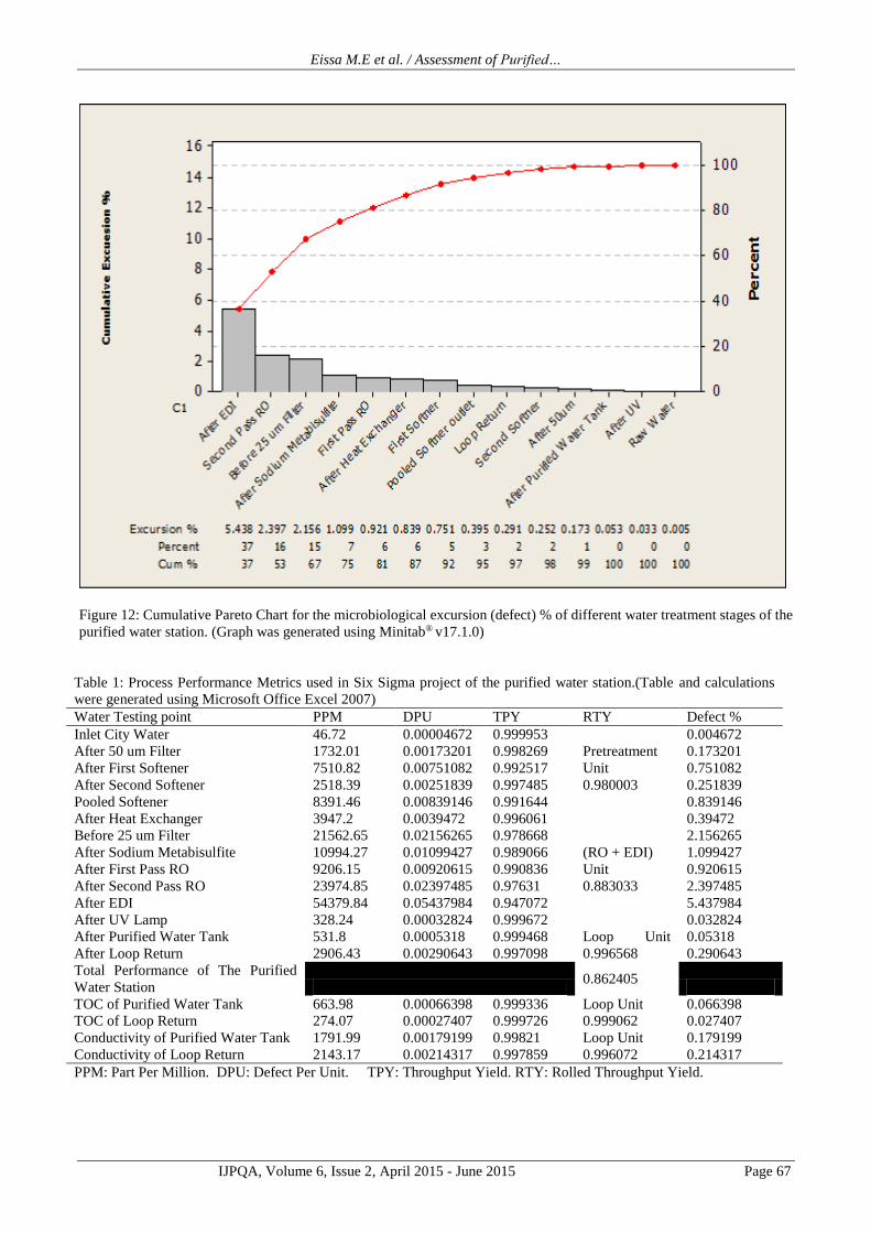
years of the study. Cumulative Pareto Chart presented in

Figure (12) demonstrates that 87% of the microbiological

defect was a resultof RO-EDI compartment contamination

with EDI unit contributing alone for 37% of the excursions

while 2% only resulted from the loop and distribution

system but PRT accounted for 11% of the defects.On the

other hand, process performance metrics shown in Table

(1) confirmed the results obtained from cumulative Pareto

chart in terms of defects and throughputs. One-Way

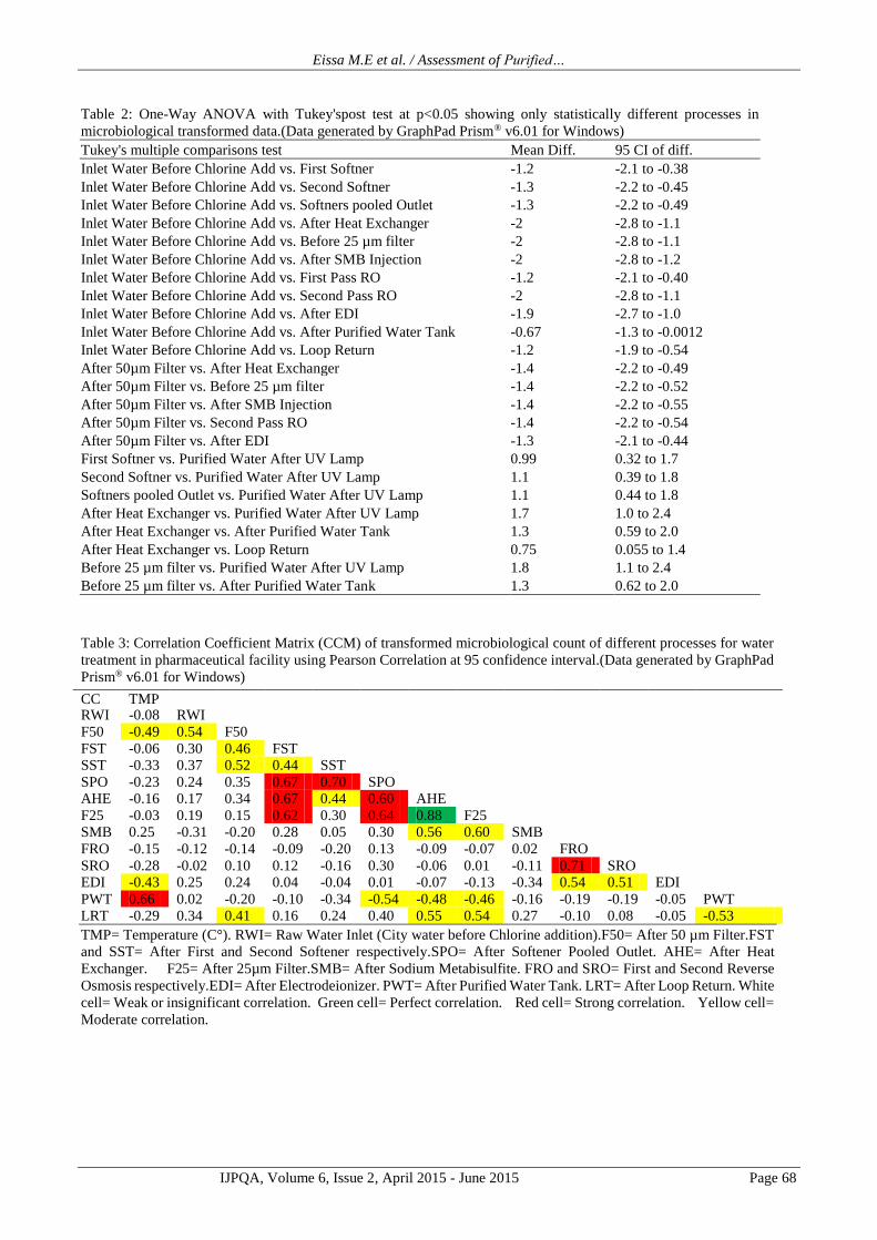
ANOVA analysis in Table (2) showed that microbial count

was raised significantly after 50 µm filter till reaching

highest counts in RO-EDI compartment which declined

significantly after UV unit.The relatedness of processing

stages microbiologically is illustrated in Table (3) showing

an interesting strong correlation between the seasonal

temperature variation and bioburden of storage tank.

Similarly, the same observation was recorded for pooled

softner output with heat exchanger and before 25 µm filter.

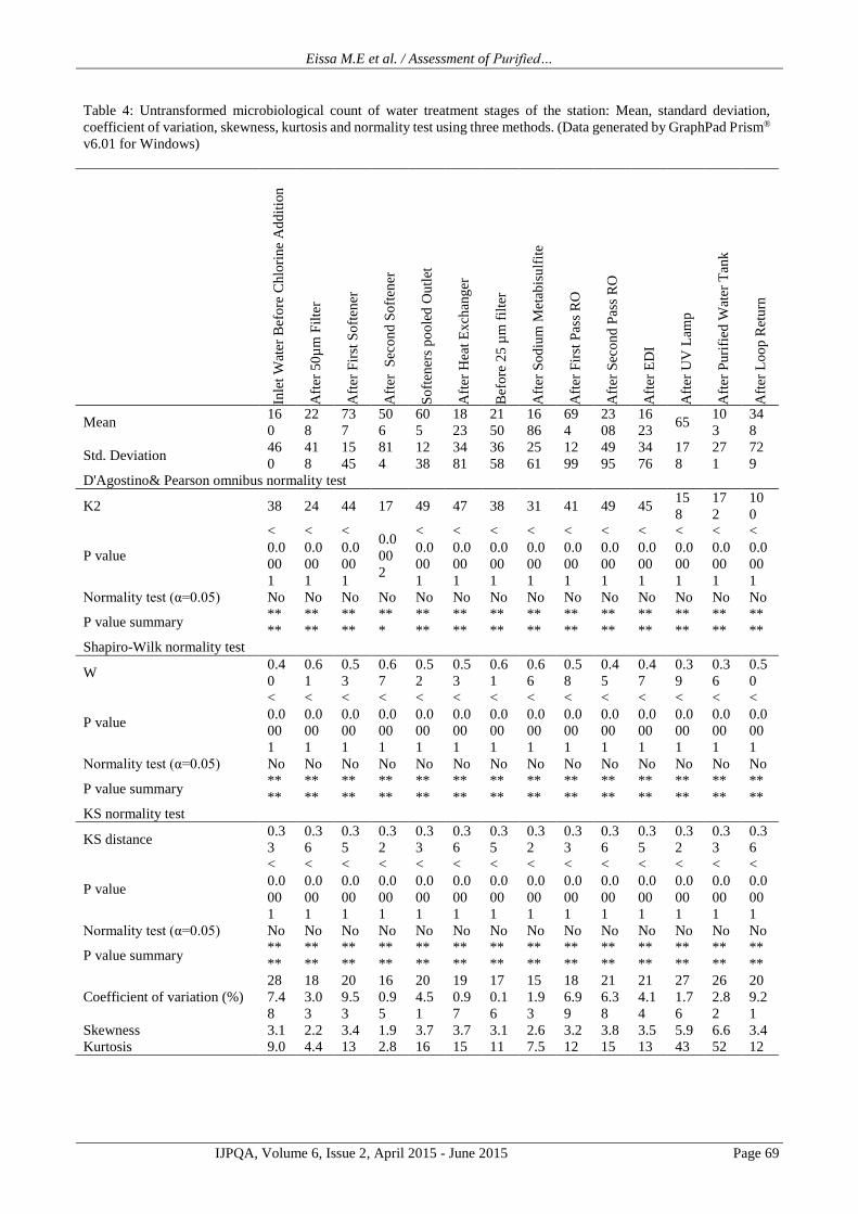
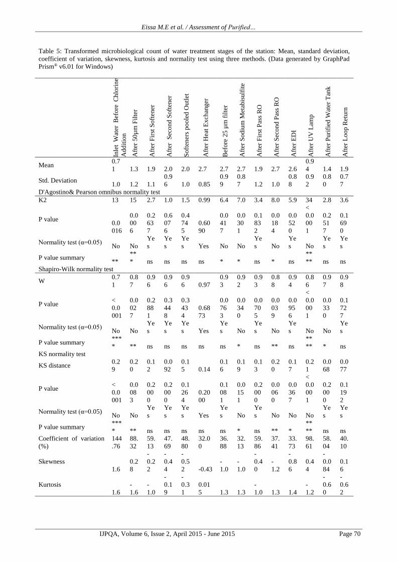
The process of data transformation had improved

normalization of the results. This finding is illustrated in

Tables (4), (5) and (6).

DISCUSSION

Wateristhemostwidelyusedingredientinpharmaceuticalma

nufacturingandthebasic component required for equipment

and system cleaning. However, controlling its microbial

quality is difficult being obtained from either municipal or

non-municipal water systems, which represents the major

exogenous source of microbial contamination of

pharmaceutical waters. It is estimated that there are70

different types of bacteria in waste water 9. Interestingly,

several different types of microbes cancross

watertreatment barriers and are found in pharmaceutical

waters 10. It is therefore not surprising that proper control

and monitoring of income water as raw material are crucial

to ensure acceptable quality of the produced water.

The observed low values of performance indices below the

reference acceptable value (1.33) are indicative that

microbiological qualities of water at different stages are in

a state of "out-of-control". By reviewing the

microbiological defenses of the water station, it was found

that at the PRT partition the first protecting mechanism

was not adequate since the antimicrobial activity of

Chlorine was set at about 600 mV measured by oxidation

reduction potential (ORP) sensor while it is recommended

to be 800 mV by the manufacturer. Moreover,an earlier

study 11 demonstrated that the microbial survival declined

significantly when ORP increased from below 620 mV to

more than 665 mV. For instance Listeria monocytogenes

survival time significantly reduced by more than 10 times,

Salmonella spp. dramatically by more than 15 times and

interestingly more than 5760 times for thermo-tolerant

coliform. In addition RO membrane that was faced with

low quality water provides good media for microbial

colonization and possible biofilm (known as membrane

fouling) formation as warned by the manufacturer.

The second defense system against microbial

contaminationis the UV lamp control after EDI unit in RO-

EDI compartment. Although the 6 UV lamps worked and

maintained appropriately during the period of study, yet it

masked the hidden defect as it disinfected water terminally

before its passage to the distribution and storage system.

Points of weakness in water station must be considered as

they could contribute to failure in water processing.

Perforated heat exchangers can also lead to direct

contamination of the water system. The FDA technical

guide, Heat Exchangers to Avoid Contamination,

discusses the design and potential problems associated

with heatexchangers12. The guide references two main

methods for preventing water contamination by leakage:

(a) provide gauges to constantly monitor pressure

differentials in order to ensure that the higher pressure is

always on the clean fluid side and (b) utilize the double-

tube sheet type heat exchanger. Also,as a preventive

measure, the FDA recommends that heat exchangers must

not be drained of the cooling water when not in use to

prevent pin holes formation in the tubing after they are

drained as a result of corrosion of the stainless steel tubes

in the presence of moisture and air. As stated by WHO 2,

ambient-temperature systems such as ion exchange, RO

and ultrafiltrationare especially susceptible to

microbiological contamination, particularly when

equipment is static during periods of no or low demand for

water. It is essential to consider the mechanisms for

microbiological control and sanitization.Special care

should be taken to control microbiological contamination

of sand filters, carbon beds and water softeners. Once

microorganisms have infected a system, the contamination

can rapidly form biofilms and spread throughout the

system. Thus unacceptable level of PRT unit may be

viewed as the source of the low efficacy of RO-EDI

partition in the current case Techniques for controlling

contamination such as back-flushing, chemical and/or

thermal sanitization and frequent regeneration should be

considered as appropriate.

The term "Normal distribution approach" has been

describedin The PDA Technical Report 13 as a method that

calculates the alert level as the mean plus twice the

standard deviation (2SD), and the action level as the mean

plus three times the standard deviation (3SD) of a

population of data points. This method suits a population

with high microbial counts best.In the current study,

thiswas applicable for purified water where relatively high

counts are expected. However, microbial population is not

normally distributed 14 so the logarithm transformation to

the base 10 for microbial count improved the

normalization process 15. In such case, alert and action

levels could be calculated from the control charts provided



that continual trending of data are ensured, updated values

of the levels could be calculated. An earlier study 14demonstrated that microbial count increased in summer

months in PW station. This was in agreement with the

finding in the current study which showed that microbial

count in the pooled purified water in storage tank is

strongly correlated with seasonal temperature variation.

Most other significant correlations are normally expected

since they were found in the related sequential processing

stages.

Figure 1: Capability sixpack using quality tools in Minitab® v17.1.0for Log10 transformed microbiological count of both city

water before NaOCl injection and after 50 µm filter cartridge in the PRT unit to approximate the normal distribution


IJPQA, Volume 6, Issue 2, April 2015 - June 2015 8

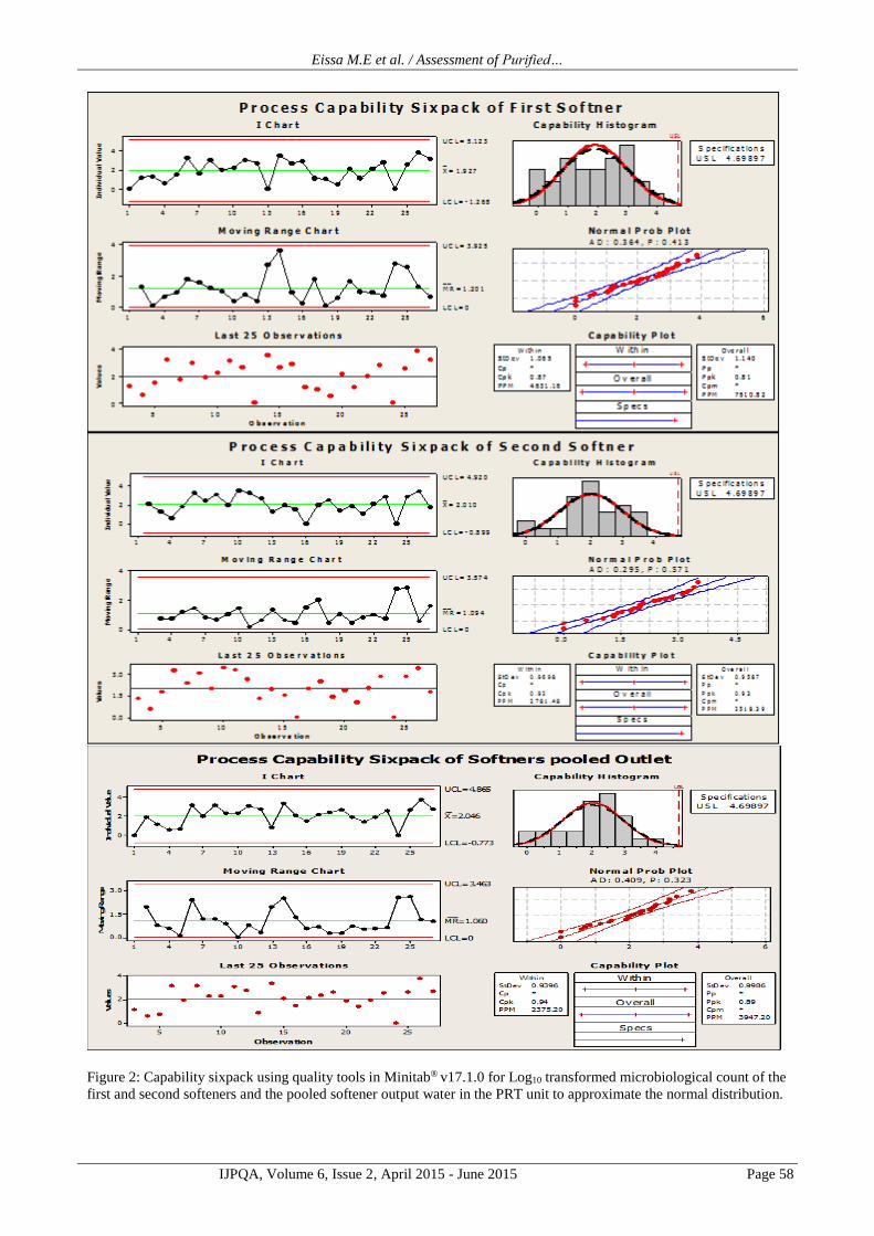
Figure 2: Capability sixpack using quality tools in Minitab® v17.1.0 for Log10 transformed microbiological count of the

first and second softeners and the pooled softener output water in the PRT unit to approximate the normal distribution.



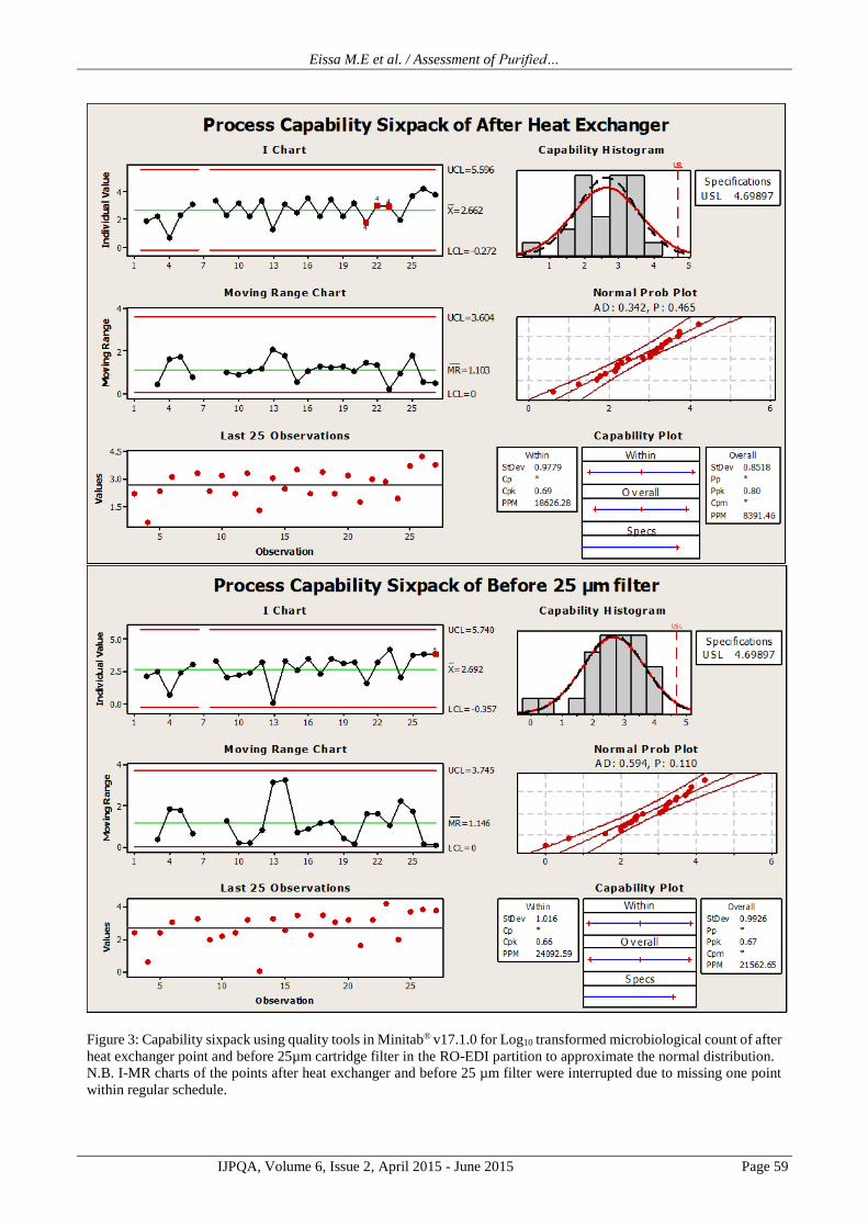
Figure 3: Capability sixpack using quality tools in Minitab® v17.1.0 for Log10 transformed microbiological count of after

heat exchanger point and before 25µm cartridge filter in the RO-EDI partition to approximate the normal distribution.

N.B. I-MR charts of the points after heat exchanger and before 25 µm filter were interrupted due to missing one point

within regular schedule.



Figure 4: Capability sixpack using quality tools in Minitab® v17.1.0 for Log10 transformed microbiological count of

point after SMB injection and the first and second pass ROs units in the RO-EDI partition to approximate the normal

distribution.



.

Figure 5: Capability sixpack using quality tools in Minitab® v17.1.0 for Log10 transformed microbiological count of

point next to EDI unit and after UV station in the RO-EDI partition to approximate the normal distribution



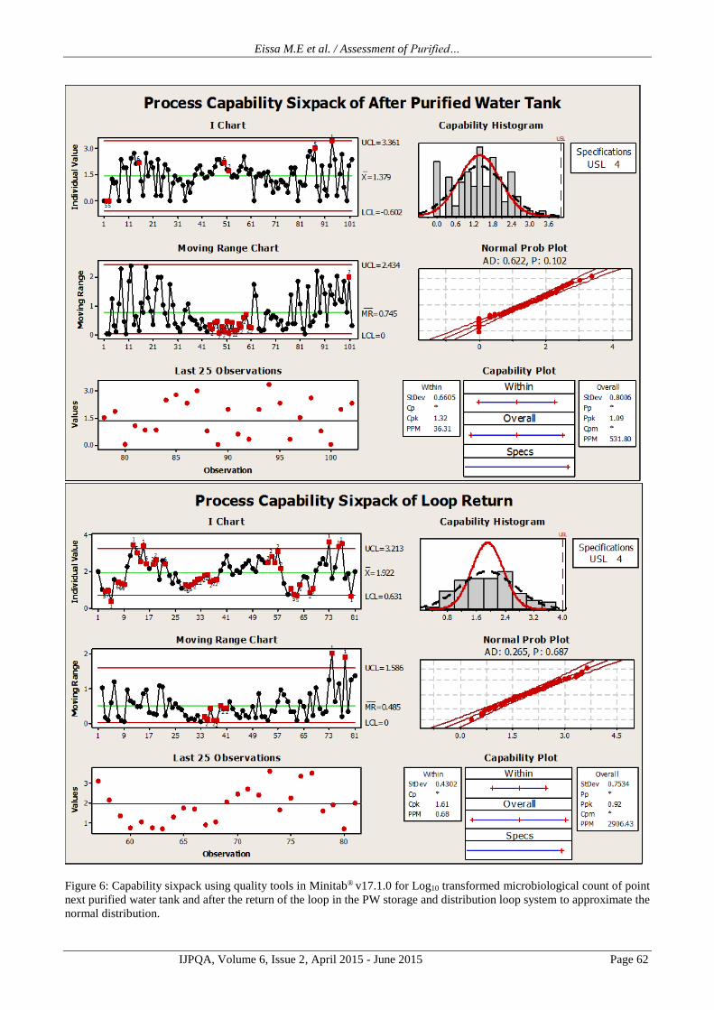
Figure 6: Capability sixpack using quality tools in Minitab® v17.1.0 for Log10 transformed microbiological count of point

next purified water tank and after the return of the loop in the PW storage and distribution loop system to approximate the

normal distribution.



Figure 7: Capability sixpack using quality tools in Minitab® v17.1.0 for Log10 transformed data of conductivity at 25°C

and TOC of after purified water storage tank (AT) point in the PW storage and distribution loop system to approximate the

normal distribution. N.B. I-MR charts of conductivity and TOC of AT point were interrupted due to missing one point

within regular schedule.



Figure 8: Capability sixpack using quality tools in Minitab® v17.1.0 for Log10 transformed data of conductivity at 25°C

and TOC of the loop return (LR) point in the PW storage and distribution loop system to approximate the normal

distribution.



Figure 9:Box-and-Whisker diagram with asterisks (*) representing outlier values, spacing between the different parts of

the box indicates the degree of dispersion and skewness in the data and whiskers indicating variability outside the upper

and lower quartiles. (Graph was generated using Minitab® v17.1.0)

Figure 10: Weight of the fractions of transformed data in about one year period from the total of those gathered during two

years period. The period covers time range duration from about 4.5 to 18 months from the study initiation. (Selection of

the fraction-time period was based on GraphPad Prism® v6.01 for Windows)



Figure 11: Different parameters and processes measured for water treatment by the facility during two years period showing

general trend line for each monitored microbiological parameter (indicated by straight line). (Figures were generated using

Microsoft Office Excel 2007)



Figure 12: Cumulative Pareto Chart for the microbiological excursion (defect) % of different water treatment stages of the

purified water station. (Graph was generated using Minitab® v17.1.0)

Table 1: Process Performance Metrics used in Six Sigma project of the purified water station.(Table and calculations

were generated using Microsoft Office Excel 2007)

Water Testing point PPM DPU TPY RTY Defect %

Inlet City Water 46.72 0.00004672 0.999953

Pretreatment

Unit

0.980003

0.004672

After 50 um Filter 1732.01 0.00173201 0.998269 0.173201

After First Softener 7510.82 0.00751082 0.992517 0.751082

After Second Softener 2518.39 0.00251839 0.997485 0.251839

Pooled Softener 8391.46 0.00839146 0.991644 0.839146

After Heat Exchanger 3947.2 0.0039472 0.996061

(RO + EDI)

Unit

0.883033

0.39472

Before 25 um Filter 21562.65 0.02156265 0.978668 2.156265

After Sodium Metabisulfite 10994.27 0.01099427 0.989066 1.099427

After First Pass RO 9206.15 0.00920615 0.990836 0.920615

After Second Pass RO 23974.85 0.02397485 0.97631 2.397485

After EDI 54379.84 0.05437984 0.947072 5.437984

After UV Lamp 328.24 0.00032824 0.999672 0.032824

After Purified Water Tank 531.8 0.0005318 0.999468 Loop Unit

0.996568

0.05318

After Loop Return 2906.43 0.00290643 0.997098 0.290643

Total Performance of The Purified

Water Station 0.862405

TOC of Purified Water Tank 663.98 0.00066398 0.999336 Loop Unit

0.999062

0.066398

TOC of Loop Return 274.07 0.00027407 0.999726 0.027407

Conductivity of Purified Water Tank 1791.99 0.00179199 0.99821 Loop Unit

0.996072

0.179199

Conductivity of Loop Return 2143.17 0.00214317 0.997859 0.214317

PPM: Part Per Million. DPU: Defect Per Unit. TPY: Throughput Yield. RTY: Rolled Throughput Yield.



Table 3: Correlation Coefficient Matrix (CCM) of transformed microbiological count of different processes for water

treatment in pharmaceutical facility using Pearson Correlation at 95 confidence interval.(Data generated by GraphPad

Prism® v6.01 for Windows)

CC

M

TMP RWI -0.08 RWI

F50 -0.49 0.54 F50

FST -0.06 0.30 0.46 FST SST -0.33 0.37 0.52 0.44 SST

SPO -0.23 0.24 0.35 0.67 0.70 SPO AHE -0.16 0.17 0.34 0.67 0.44 0.60 AHE

F25 -0.03 0.19 0.15 0.62 0.30 0.64 0.88 F25 SMB 0.25 -0.31 -0.20 0.28 0.05 0.30 0.56 0.60 SMB

FRO -0.15 -0.12 -0.14 -0.09 -0.20 0.13 -0.09 -0.07 0.02 FRO

SRO -0.28 -0.02 0.10 0.12 -0.16 0.30 -0.06 0.01 -0.11 0.71 SRO EDI -0.43 0.25 0.24 0.04 -0.04 0.01 -0.07 -0.13 -0.34 0.54 0.51 EDI

PWT 0.66 0.02 -0.20 -0.10 -0.34 -0.54 -0.48 -0.46 -0.16 -0.19 -0.19 -0.05 PWT LRT -0.29 0.34 0.41 0.16 0.24 0.40 0.55 0.54 0.27 -0.10 0.08 -0.05 -0.53

TMP= Temperature (C°). RWI= Raw Water Inlet (City water before Chlorine addition).F50= After 50 µm Filter.FST

and SST= After First and Second Softener respectively.SPO= After Softener Pooled Outlet. AHE= After Heat

Exchanger. F25= After 25µm Filter.SMB= After Sodium Metabisulfite. FRO and SRO= First and Second Reverse

Osmosis respectively.EDI= After Electrodeionizer. PWT= After Purified Water Tank. LRT= After Loop Return. White

cell= Weak or insignificant correlation. Green cell= Perfect correlation. Red cell= Strong correlation. Yellow cell=

Moderate correlation.

Table 2: One-Way ANOVA with Tukey'spost test at p<0.05 showing only statistically different processes in

microbiological transformed data.(Data generated by GraphPad Prism® v6.01 for Windows)

Tukey's multiple comparisons test Mean Diff. 95 CI of diff.

Inlet Water Before Chlorine Add vs. First Softner -1.2 -2.1 to -0.38

Inlet Water Before Chlorine Add vs. Second Softner -1.3 -2.2 to -0.45

Inlet Water Before Chlorine Add vs. Softners pooled Outlet -1.3 -2.2 to -0.49

Inlet Water Before Chlorine Add vs. After Heat Exchanger -2 -2.8 to -1.1

Inlet Water Before Chlorine Add vs. Before 25 µm filter -2 -2.8 to -1.1

Inlet Water Before Chlorine Add vs. After SMB Injection -2 -2.8 to -1.2

Inlet Water Before Chlorine Add vs. First Pass RO -1.2 -2.1 to -0.40

Inlet Water Before Chlorine Add vs. Second Pass RO -2 -2.8 to -1.1

Inlet Water Before Chlorine Add vs. After EDI -1.9 -2.7 to -1.0

Inlet Water Before Chlorine Add vs. After Purified Water Tank -0.67 -1.3 to -0.0012

Inlet Water Before Chlorine Add vs. Loop Return -1.2 -1.9 to -0.54

After 50µm Filter vs. After Heat Exchanger -1.4 -2.2 to -0.49

After 50µm Filter vs. Before 25 µm filter -1.4 -2.2 to -0.52

After 50µm Filter vs. After SMB Injection -1.4 -2.2 to -0.55

After 50µm Filter vs. Second Pass RO -1.4 -2.2 to -0.54

After 50µm Filter vs. After EDI -1.3 -2.1 to -0.44

First Softner vs. Purified Water After UV Lamp 0.99 0.32 to 1.7

Second Softner vs. Purified Water After UV Lamp 1.1 0.39 to 1.8

Softners pooled Outlet vs. Purified Water After UV Lamp 1.1 0.44 to 1.8

After Heat Exchanger vs. Purified Water After UV Lamp 1.7 1.0 to 2.4

After Heat Exchanger vs. After Purified Water Tank 1.3 0.59 to 2.0

After Heat Exchanger vs. Loop Return 0.75 0.055 to 1.4

Before 25 µm filter vs. Purified Water After UV Lamp 1.8 1.1 to 2.4

Before 25 µm filter vs. After Purified Water Tank 1.3 0.62 to 2.0



Table 4: Untransformed microbiological count of water treatment stages of the station: Mean, standard deviation,

coefficient of variation, skewness, kurtosis and normality test using three methods. (Data generated by GraphPad Prism®

v6.01 for Windows)

In

let

Wat

er B

efo

re C

hlo

rin

e A

dd

itio

n

Aft

er 5

0µ

m F

ilte

r

Aft

er F

irst

So

ften

er

Aft

er

Sec

on

d S

oft

ener

So

ften

ers

po

ole

d O

utl

et

Aft

er H

eat

Ex

chan

ger

Bef

ore

25

µm

fil

ter

Aft

er S

od

ium

Met

abis

ulf

ite

Aft

er F

irst

Pas

s R

O

Aft

er S

eco

nd

Pas

s R

O

Aft

er E

DI

Aft

er U

V L

amp

Aft

er P

uri

fied

Wat

er T

ank

Aft

er L

oo

p R

etu

rn

Mean 16

0

22

8

73

7

50

6

60

5

18

23

21

50

16

86

69

4

23

08

16

23 65

10

3

34

8

Std. Deviation 46

0

41

8

15

45

81

4

12

38

34

81

36

58

25

61

12

99

49

95

34

76

17

8

27

1

72

9

D'Agostino& Pearson omnibus normality test

K2 38 24 44 17 49 47 38 31 41 49 45 15

8

17

2

10

0

P value

<

0.0

00

1

<

0.0

00

1

<

0.0

00

1

0.0

00

2

<

0.0

00

1

<

0.0

00

1

<

0.0

00

1

<

0.0

00

1

<

0.0

00

1

<

0.0

00

1

<

0.0

00

1

<

0.0

00

1

<

0.0

00

1

<

0.0

00

1

Normality test (α=0.05) No No No No No No No No No No No No No No

P value summary **

**

**

**

**

**

**

*

**

**

**

**

**

**

**

**

**

**

**

**

**

**

**

**

**

**

**

**

Shapiro-Wilk normality test

W 0.4

0

0.6

1

0.5

3

0.6

7

0.5

2

0.5

3

0.6

1

0.6

6

0.5

8

0.4

5

0.4

7

0.3

9

0.3

6

0.5

0

P value

<

0.0

00

1

<

0.0

00

1

<

0.0

00

1

<

0.0

00

1

<

0.0

00

1

<

0.0

00

1

<

0.0

00

1

<

0.0

00

1

<

0.0

00

1

<

0.0

00

1

<

0.0

00

1

<

0.0

00

1

<

0.0

00

1

<

0.0

00

1


P value summary **

**

**

**

**

**

**

**

**

**

**

**

**

**

**

**

**

**

**

**

**

**

**

**

**

**

**

**

KS normality test

KS distance 0.3

3

0.3

6

0.3

5

0.3

2

0.3

3

0.3

6

0.3

5

0.3

2

0.3

3

0.3

6

0.3

5

0.3

2

0.3

3

0.3

6

P value

<

0.0

00

1

<

0.0

00

1

<

0.0

00

1

<

0.0

00

1

<

0.0

00

1

<

0.0

00

1

<

0.0

00

1

<

0.0

00

1

<

0.0

00

1

<

0.0

00

1

<

0.0

00

1

<

0.0

00

1

<

0.0

00

1

<

0.0

00

1


P value summary **

**

**

**

**

**

**

**

**

**

**

**

**

**

**

**

**

**

**

**

**

**

**

**

**

**

**

**

Coefficient of variation (%)

28

7.4

8

18

3.0

3

20

9.5

3

16

0.9

5

20

4.5

1

19

0.9

7

17

0.1

6

15

1.9

3

18

6.9

9

21

6.3

8

21

4.1

4

27

1.7

6

26

2.8

2

20

9.2

1

Skewness 3.1 2.2 3.4 1.9 3.7 3.7 3.1 2.6 3.2 3.8 3.5 5.9 6.6 3.4

Kurtosis 9.0 4.4 13 2.8 16 15 11 7.5 12 15 13 43 52 12



Table 5: Transformed microbiological count of water treatment stages of the station: Mean, standard deviation,

coefficient of variation, skewness, kurtosis and normality test using three methods. (Data generated by GraphPad

Prism® v6.01 for Windows)

In

let

Wat

er B

efo

re C

hlo

rin

e

Ad

dit

ion

Aft

er 5

0µ

m F

ilte

r

Aft

er F

irst

So

ften

er

Aft

er

Sec

on

d S

oft

ener

So

ften

ers

po

ole

d O

utl

et

Aft

er H

eat

Ex

chan

ger

Bef

ore

25

µm

fil

ter

Aft

er S

od

ium

Met

abis

ulf

ite

Aft

er F

irst

Pas

s R

O

Aft

er S

eco

nd

Pas

s R

O

Aft

er E

DI

Aft

er U

V L

amp

Aft

er P

uri

fied

Wat

er T

ank

Aft

er L

oo

p R

etu

rn

Mean 0.7

1 1.3 1.9 2.0 2.0 2.7 2.7 2.7 1.9 2.7 2.6

0.9

4 1.4 1.9

Std. Deviation 1.0 1.2 1.1

0.9

6 1.0 0.85

0.9

9

0.8

7 1.2 1.0

0.8

8

0.9

2

0.8

0

0.7

7


K2 13 15 2.7 1.0 1.5 0.99 6.4 7.0 3.4 8.0 5.9 34 2.8 3.6

P value 0.0

016

0.0

00

6

0.2

63

7

0.6

07

6

0.4

74

5

0.60

90

0.0

41

7

0.0

30

1

0.1

83

2

0.0

18

4

0.0

52

0

<

0.0

00

1

0.2

51

7

0.1

69

0

Normality test (α=0.05) No No

Ye

s

Ye

s

Ye

s Yes No No

Ye

s No

Ye

s No

Ye

s

Ye

s

P value summary **

**

* ns ns ns ns * * ns * ns

**

** ns ns


W 0.7

1

0.8

7

0.9

6

0.9

6

0.9

6 0.97

0.9

3

0.9

2

0.9

3

0.8

8

0.9

4

0.8

6

0.9

7

0.9

8

P value <

0.0

001

0.0

02

7

0.2

88

1

0.3

44

8

0.3

43

4

0.68

73

0.0

76

3

0.0

34

0

0.0

70

5

0.0

03

9

0.0

95

6

<

0.0

00

1

0.0

33

0

0.1

72

7


Ye

s

Ye

s

Ye

s Yes

Ye

s No

Ye

s No

Ye

s No No

Ye

s

P value summary ***

* ** ns ns ns ns ns * ns ** ns

**

** * ns

KS normality test

KS distance 0.2

9

0.2

0

0.1

2

0.0

92

0.1

5 0.14

0.1

6

0.1

9

0.1

3

0.2

0

0.1

7

0.2

1

0.0

68

0.0

77

P value <

0.0

001

0.0

08

3

0.2

00

0

0.2

00

0

0.1

26

4

0.20

00

0.1

08

1

0.0

15

1

0.2

00

0

0.0

06

0

0.0

36

7

<

0.0

00

1

0.2

00

0

0.1

19

2


Ye

s

Ye

s

Ye

s Yes

Ye

s No

Ye

s No No No

Ye

s

Ye

s

P value summary ***

* ** ns ns ns ns ns * ns ** *

**

** ns ns

Coefficient of variation

(%)

144

.76

88.

32

59.

13

47.

69

48.

80

32.0

0

36.

88

32.

13

59.

86

37.

41

33.

73

98.

61

58.

04

40.

10

Skewness

1.6

0.2

8

-

0.2

2

-

0.4

4

-

0.5

2 -0.43

-

1.0

-

1.0

-

0.4

0

-

1.2

-

0.8

6

0.4

4

-

0.0

84

0.1

6

Kurtosis

1.6

-

1.6

-

1.0

-

0.1

9

-

0.3

1

0.01

5 1.3 1.3

-

1.0 1.3 1.4

-

1.2

-

0.6

0

-

0.6

2



Finally, Systems that operate and are maintained at

elevated temperatures, in the range of 70–80°C (as in the

current case), are generally less susceptible to

microbiological contamination than systems that are

maintained at lower temperatures. When lower

temperatures are required due to the water treatment

processes employed or the temperature requirements for

the water in use, then special precautions should be taken

to prevent the ingress and proliferation of microbiological

contaminants 16. Even though, inappropriate control,

maintenance and sanitization can lead to catastrophic

excursions in water quality which may lead to sever

financial loss and more importantly health hazard risk.

REFERENCES

1. Notes for Guidance on Quality of Water for

Pharmaceutical Use, The European Agency for the

Evaluation of Medicinal Products (EMEA),

London,May 2002.

2. http://www.ema.europa.eu/docs/en_GB/document_lib

rary/Scientific_guideline/2009/09/WC500003394.pdf

3. WHO good manufacturing practices: water for

pharmaceutical useAnnex 2revision of WHO Technical

Report Series, No. 929, Annex 3,

2005http://apps.who.int/prequal/info_general/docume

nts/TRS970/TRS_970_Annex2.pdf

Table 6: Untransformed and logarithmically transformed conductivity at 25°C, total organic carbon (TOC) and climatic

temperature (°C) data of the water treatment station: Mean, standard deviation, coefficient of variation, skewness,

kurtosis and normality test using three methods. (Data generated by GraphPad Prism® v6.01 for Windows)

Untransformed Data Transformed Data

Lo

op

Ret

urn

Co

nd

uct

ivit

y

Lo

op

Ret

urn

TO

C

Pu

rifi

ed W

ater

Tan

k C

ond

uct

ivit

y

Pu

rifi

ed W

ater

Tan

k T

OC

Cli

mat

ic T

emp

erat

ure

Lo

op

Ret

urn

Co

nd

uct

ivit

y

Lo

op

Ret

urn

TO

C

Pu

rifi

ed W

ater

Tan

k C

ond

uct

ivit

y

Pu

rifi

ed W

ater

Tan

k T

OC

Cli

mat

ic T

emp

erat

ure

Mean 0.65 81 0.65 82 23 0.22 1.8 0.21 1.8 1.4

Std. Deviation 0.19 50 0.19 52 5.4 0.052 0.26 0.051 0.27 0.11


K2 4.3 14 2.3 16 40 4.4 6.4 2.7 6.7 14

P value 0.114

6

0.000

9

0.324

3

0.000

3

<

0.000

1

0.111

5

0.041

6

0.265

1

0.035

4

0.001

0

Normality test (α=0.05) Yes No Yes No No Yes No Yes No No

P value summary ns *** ns *** **** ns * ns * ***


W 0.98 0.88 0.98 0.88 0.94 0.97 0.97 0.98 0.97 0.92

P value 0.127

4

<

0.000

1

0.409

1

<

0.000

1

<

0.000

1

0.021

7

0.088

9

0.119

1

0.097

2

<

0.000

1

Normality test (α=0.05) Yes No Yes No No No Yes Yes Yes No

P value summary ns **** ns **** **** * ns ns ns ****

KS normality test

KS distance 0.094 0.16 0.085 0.14 0.12 0.11 0.084 0.10 0.090 0.14

P value 0.058

8

0.000

2

0.123

7

0.002

8

0.000

4

0.011

3

0.200

0

0.028

5

0.189

1

<

0.000

1

Normality test (α=0.05) Yes No Yes No No No Yes No Yes No

P value summary ns *** ns ** *** * ns * ns ****

Coefficient of variation (%) 29.16 62.16 29.22 63.79 23.58 23.93 14.35 23.82 14.66 7.71

Skewness -0.29 1.1 -0.14 1.2 -0.28 -0.52 0.064 -0.39 0.075 -0.56

Kurtosis -0.67 0.95 -0.59 1.4 -1.2 -0.34 -0.92 -0.35 -0.94 -0.85



4. Potdar MA; Pharmaceutical Quality Assurance. 2nd

Edition, Nirali .. Press Publication, Delhi, December

2007: 8.2-8.3. 11

5. 2015 USPC Official 12-1-14 - 04-30-15 General

Chapters <1231>Water for pharmaceutical purposes.

6. Design for Six Sigma LeanToolset: Implementing

Innovations Successfully Christian Staudter،Jens-Peter

Mollenhauer،RenataMeran،Olin Roenpage،Clemens

Hugo, Alexis Hamalides,

7. Eissa, M. Studies of Microbial Resistance Against

Some Disinfectants, Lambert Academic Publishing,

2014.

8. National Primary Drinking Water Regulations

(NPDWR; 2006), United States Environmental

Protection Agency.

9. Sutton SV, Proud DW, Rachui S, Brannan DK.

Validation of microbial recovery from

disinfectants.PDA J Pharm Sci Technol. 2002; 56(5):

255-266.

10. Traeger, H. Pharmaceuticals, The Presence of Bacteria,

Endotoxins, and Biofilms in Pharmaceutical Water,

Ultrapure Water, March 2003.

11. Clontz, L. Microbial Limit and Bioburden Tests:

Validation Approaches and Global Requirements, 2nd

Edition, CRC press, 2008.

12. Suslow. TV. Oxidation Reduction Potenial (ORP) for

Water Disinfection Monitoring, Control and

Documentation Publication 8149.

http://anrcatalog.ucdavis.edu/pdf/8149.pdf

13. FDA Technical Guide Heat Exchangers to Avoid

Contamination, Department of Health and Education

and Welfare Public Health Service, Food and Drug

Administration, No. 34, 1979.

14. PDA Technical Report No. 13. Fundamentals of an

Environmental Monitoring Program, Parenteral Drug

Association, Bethesda, MD. 1990.

15. Sandle, T (2004) An approach for the reporting of

microbiological results from water systems. PDA J

Pharm SciTechnol 58: 4. 231-237.

16. Sokal, RR, Rohlf, FJ. Biometry: The Principles and

Practice of Statistics in Biological Research. 4th

edition, W.H. Freeman and Co, New York, 1995.

17. Choudhary, A. WHO: water for Pharmaceutical Use,

2008. http://www.pharmaguideline.com/2010/12/who-

water-for-pharmaceutical-use.html

assessment of purified water quality in pharmaceutical...

Documents