assessment of the impact of land subsidence, sea …adpc.net/casita/case_studies/coastal hazard...
TRANSCRIPT

Land Subsidence & Sea Level Rise in Semarang Damen & Sutanta
ILWIS 3.1 Exercise Semarang -ILWIS Lesson Ver.04.doc Page 1
Assessment of the Impact of Land Subsidence, Sea Level Rise and Coastal Change in the city of Semarang, Java, Indonesia
M.C.J. DAMEN *) and H. SUTANTA **) *) Dept. of Environmental System Analysis, International Institute Geo-Information Science and Earth Observation (ITC), P.O. Box 6, 7500 AA Enschede, The Netherlands. Tel: +31 (0)53 4874266, Fax: +31 (0)53 4874336; e-mail: [email protected] **) Dept. of Geodetic Engineering, Gadjah Mada University, J. Grafika, no.2, Jogyakarta, Indonesia Tel : 62 274902 121; Fax : 62 274 520226; e-mail: [email protected]
Summary & background The exercise deals with the use of GIS and Remote Sensing for the study of the impact of land subsidence and sea level rise in the city of Semarang, Central java, Indonesia. Semarang city is suffering from two types of flooding, from rivers and high tides. The extend and magnitude of the floods seriously increased in recent years. This appears to be related to the ongoing processes of land subsidence and global sea level rise that this coastal city is faced with. The rate of subsidence in the city is varying, up to a maximum of 12 cm/yr. Medium estimates of sea level rise in the region indicate that the sea level in Indonesia will rise by 9, 13, and 45 cm for the years 2010, 2019, and 2070 respectively. To assess the combined effect of these phenomena and its spatial distribution, a procedure has to be applied which combines up-to-date geo-information sources on terrain elevation and land use. In the exercise, a high accuracy Digital Elevation Model (DEM) will be generated using a point map of photo-grammetrically-derived data. The present land use in the area will be assessed using high-resolution satellite imagery of Landsat-7 ETM+ and ASTER bands 1 - 3. Also available is a scanned topographical map of the area and hazard maps of the present flooding of river and from the sea. In the exercise the student will calculate the impact of land subsidence and sea level rise on land use and population in a GIS environment. It aims to be applicable to other ‘sinking cities’ as well. The exercise will produce several maps of the coastline change in the period 1867 – 2001, elevation of the land relative to the average sea level in 2010, 2019 and 2070 abd tables of the elements at risk, such as the population, industrial areas and main roads. The methodology for the exercise has been derived from:
− Heri Sutanta (2002) - “Spatial modeling of the Impact of Land Subsidence and Sea Level Rise in a Coastal Urban Setting”, ITC-MSc study.
Additional background information on the study is given in the article: SUTANTA, H ET AL., 2002 - Preliminary Assessment of the Impact of Land Subsidence and Sea Level Rise in Semarang, Central Java, Indonesia See Appendix-2. It is recommended to read the article before starting the exercise.

Land Subsidence & Sea Level Rise in Semarang Damen & Sutanta
ILWIS 3.1 Exercise Semarang -ILWIS Lesson Ver.04.doc Page 2
Available data for the exercise
File name File contents Satellite images
MSS72b1,…b2,…b3,…b4
Raster map of the Landsat MSS image of 23 September 1972, bands 1 � 4. Resolution of all bands: 79m.
ETM01b1,…b2,…b3,…b4, …b5,…b8
Raster map of the Enhanced Thematic-Mapper image of 2th August 2001, bands 1 �5 and band 8. Resolution bands 1 � 5 is 30m and of band 8: 15 m.
ASTER01b1,…b2,…b3 Raster Map of ASTER-1B image of 16 February 2001, bands 1 � 3, with a resolution of 15m.
Topographical maps
Topo_1871, Topo_1908, Topo_1937, Topo_1992
Scanned topographical maps of the years 1871, 1908, 1937 and 1992 with a pixel resolution of 5.
Point, segment and
polygon maps
Administration Segment and polygon maps of the administrative subdivision of the city of Semarang in ‘kampungs’ and the population densities in a table.
Benchmarks Point map of benchmarks with a known subsidence rate in mm per year
Eleva01 Point map of the elevations in 2001, in the central part of Semarang in meters
Industrial Segment and polygon map of industrial areas (digitized from paper map)
Coastlines Digitized Coastlines based on the topographical maps of 1871 and 1992.
Waterbodies Segment and polygon map of waterbodies, such as the Java sea, rivers and canals (digitized from topographical map)
Riverflood Segment and polygon map of river flooding (digitized from paper map)
Roads Polygon map of the main roads Robflood Segment and polygon map of rob flooding (tidal flooding) SubsMask Raster, polygon map. Mask of study area for subsidence StudyArea Segment map of the boundary of the study area. Indonesia Digital Elevation Model from the whole of Indonesia. Pixel
size approx. 900*900 m. Vertical accuracy: approx. 1m. Downloaded from GLOBEDEM website: http://www.ngdc.noaa.gov/seg/topo/globeget.shtml

Land Subsidence & Sea Level Rise in Semarang Damen & Sutanta
ILWIS 3.1 Exercise Semarang -ILWIS Lesson Ver.04.doc Page 3
LESSON 1
Introduction to ILWIS 3.1 using data from Semarang, Indonesia
ILWIS is an acronym for the Integrated Land and Water Information System. It is a Geographic Information System (GIS) with Image Processing capabilities. ILWIS has been developed by the International Institute for Geo-Information Science and Earth Observation (ITC), Enschede, The Netherlands. As a GIS package, ILWIS allows you to input, manage, analyze and present geo-graphical data. From the data you can generate information on the spatial and temporal patterns and processes on the earth surface. Geographic Information Systems are nowadays indispensable in many different fields of applications to assist in the decision making process. Most decisions are influenced by some facts of geography. What is at a certain location? Where are the most suitable sites? Where, when and which changes took place? Here are some examples.
− In land use planning, GIS is used to evaluate the consequences of different scenarios in the development of a region.
− In geology, GIS is used to find the most suitable places for mining, or to determine areas subject to natural hazards.
− Areas that may be affected by pollution are analyzed using GIS functions.
− Extensions of cities are planned, based on analysis of many spatial and temporal patterns, etc.
In order to be able to make the right decisions, access to different sorts of information is required. The data should be maintained and updated and should be used in the analysis to obtain useful information. In this process ILWIS can be an important tool. This Lesson is intended to introduce you to ILWIS, and specifically to the user interface. You will learn how to start ILWIS, the functions of the Main window and how to open maps and tables, using spatial and attribute data from Semarang, Indonesia.
Land Subsidence & Sea Level Rise in Semarang Damen & Sutanta
ILWIS 3.1 Exercise Semarang -ILWIS Lesson Ver.04.doc Page 4
1.1 Starting ILWIS
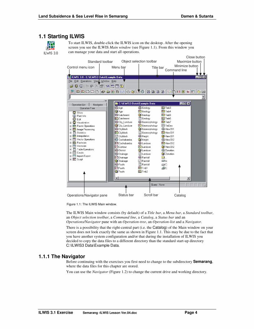
To start ILWIS, double-click the ILWIS icon on the desktop. After the opening screen you see the ILWIS Main window (see Figure 1.1). From this window you can manage your data and start all operations.
Control menu icon Title barMenu bar
Standard toolbar Object selection toolbar
Command lineMinimize button
Maximize buttonClose button
Operations/Navigator pane Status bar Scroll bar Catalog
Figure 1.1: The ILWIS Main window.
The ILWIS Main window consists (by default) of a Title bar, a Menu bar, a Standard toolbar, an Object selection toolbar, a Command line, a Catalog, a Status bar and an Operations/Navigator pane with an Operation-tree, an Operation-list and a Navigator. There is a possibility that the right-central part (i.e. the Catalog) of the Main window on your screen does not look exactly the same as shown in Figure 1.1. This may be due to the fact that you have another system configuration and/or that during the installation of ILWIS you decided to copy the data files to a different directory than the standard start-up directory C:\ILWIS3 Data\Example Data.
1.1.1 The Navigator Before continuing with the exercises you first need to change to the subdirectory Semarang, where the data files for this chapter are stored. You can use the Navigator (Figure 1.2) to change the current drive and working directory.

Land Subsidence & Sea Level Rise in Semarang Damen & Sutanta
ILWIS 3.1 Exercise Semarang -ILWIS Lesson Ver.04.doc Page 5
Figure 1.2: The ILWIS Navigator.
��
• Click the word Navigator in the Operations/Navigator pane.
The Navigator lists all drives and directories (i.e. folders) in a tree structure. The Navigator also has a History to easily return to previously visited drives and directories.
��
• Click on the drives and folders in the Navigator until you are in the directory where the data for this exrecise has been stored. The data is located in the directory Semarang.
1.1.2 Catalog(s) If you are in the correct directory Semarang you will see, that the right hand side of the Main window, looks the same as Figure 1.3. This part of the Main window, in which maps, tables and other ILWIS objects in the working directory are displayed each with its own type of icon, is called the Catalog. When you double-click an object in the Catalog, it will be displayed.
Figure 1.3: Example of a Catalog of the ILWIS Main window.
Land Subsidence & Sea Level Rise in Semarang Damen & Sutanta
ILWIS 3.1 Exercise Semarang -ILWIS Lesson Ver.04.doc Page 6
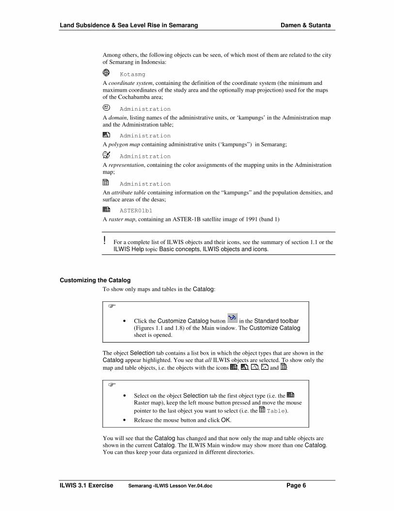
Among others, the following objects can be seen, of which most of them are related to the city of Semarang in Indonesia:
Kotasmg
A coordinate system, containing the definition of the coordinate system (the minimum and maximum coordinates of the study area and the optionally map projection) used for the maps of the Cochabamba area;
Administration
A domain, listing names of the administrative units, or ‘kampungs’ in the Administration map and the Administration table;
Administration
A polygon map containing administrative units (‘kampungs”) in Semarang;
Administration
A representation, containing the color assignments of the mapping units in the Administration map;
Administration
An attribute table containing information on the “kampungs” and the population densities, and surface areas of the desas;
ASTER01b1
A raster map, containing an ASTER-1B satellite image of 1991 (band 1)
! For a complete list of ILWIS objects and their icons, see the summary of section 1.1 or the ILWIS Help topic Basic concepts, ILWIS objects and icons.
Customizing the Catalog To show only maps and tables in the Catalog:
��
• Click the Customize Catalog button in the Standard toolbar (Figures 1.1 and 1.8) of the Main window. The Customize Catalog sheet is opened.
The object Selection tab contains a list box in which the object types that are shown in the Catalog appear highlighted. You see that all ILWIS objects are selected. To show only the map and table objects, i.e. the objects with the icons , , , and :
��
• Select on the object Selection tab the first object type (i.e. the Raster map), keep the left mouse button pressed and move the mouse pointer to the last object you want to select (i.e. the Table).
• Release the mouse button and click OK.
You will see that the Catalog has changed and that now only the map and table objects are shown in the current Catalog. The ILWIS Main window may show more than one Catalog. You can thus keep your data organized in different directories.

Land Subsidence & Sea Level Rise in Semarang Damen & Sutanta
ILWIS 3.1 Exercise Semarang -ILWIS Lesson Ver.04.doc Page 7
! You can open another Catalog by clicking the New Catalog button in the Standard toolbar and selecting a new directory. You can also select the New Catalog command on the Window menu of the Main window.
�� Position the mouse pointer on an object, for example on polygon map Administration. A description of this map will appear on the Status bar (Figure 1.7) of the Main window.
1.1.3 Title bar and Menu bar The Title bar (Figure 1.4) shows the name of the currently active Catalog. You can move a window to another position on the screen by dragging that window’s Title bar to another position.
Figure 1.4: Title bar of the ILWIS Main window. The Menu bar (Figure 1.5) can be used for example to start an operation. The ILWIS Main window has six menus: File, Edit, Operations, View, Window and Help.
Figure 1.5: The Menu bar of the Main window.
��
• Click Operations in the Menu bar. The Operations menu is opened. The menu contains commands for all ILWIS operations, which are grouped. The triangles to the right of the commands on a menu indicate that there is another cascading menu.
• Position the mouse pointer on the command Image Processing. A submenu appears.
• Select the Filter command. The Filtering dialog box is opened. In this dialog box you can select among other things the input maps for an operation.
• Close the dialog box by clicking the Cancel button.
• Open some more menus and have a look at their contents. The Status bar (at the bottom of the Main window) gives short explanations.
1.1.4 The Operation-tree and Operation-list Let us now concentrate on another part of the ILWIS Main window. The Operation-tree and the Operation-list (Figure 1.6) are located on the first two tabs in the Operations/Navigator pane, by default along the left-hand side of the Main window. - The Operation-tree provides a tree structure for all ILWIS operations, similar to the
Operations menu.
- The Operation-list contains an alphabetic list of all ILWIS operations.
In the Operation-tree as well as in the Operation-list each item is preceded by an icon. The icon indicates the output data type of the operation. By double-clicking an operation, the operation will be started. We will do this later.

Land Subsidence & Sea Level Rise in Semarang Damen & Sutanta
ILWIS 3.1 Exercise Semarang -ILWIS Lesson Ver.04.doc Page 8
Figure 1.6: ILWIS Operation-tree (left) and ILWIS Operation-list (right).
��
• In the Operation-tree, double-click Image Processing, or click on the + in front of the Image Processing icon , to expand the Image Processing tree.
• Position the mouse pointer on one of the operations, for example on the Filter operation.
1.1.5 Status bar When the mouse pointer is positioned on an operation, the Status bar (Figure 1.7), located at the bottom of the Main window, shows a short description of that operation.
Figure 1.7: The Status bar of the ILWIS Main window.
To get more information on an operation:
��
• Click in the Operation-list with the right mouse button on an operation and select Help from the context-sensitive menu. An Additional Help window appears with a short explanation of the operation.
• You can close the Additional Help window again by pressing the Close button in the Title bar of the Help window or by double-clicking the control-menu icon .
The Status bar also gives short information when you move the mouse pointer to a menu command, to a button in the Toolbar or to an object in the Catalog.
��
• Click in the Catalog with the right mouse button on polygon map Administration to get a context-sensitive menu.
A Context-sensitive menu is a menu, which gives only those menu commands that are applicable to the moment you use the right mouse button; thus you will get a different menu depending on where and when you use the right-mouse button. For example, if you use the right mouse button on a polygon map, the context-sensitive menu will only show the
Land Subsidence & Sea Level Rise in Semarang Damen & Sutanta
ILWIS 3.1 Exercise Semarang -ILWIS Lesson Ver.04.doc Page 9
operations, which can be applied on polygon maps. Context-sensitive menus are shortcuts for normal menu commands
1.1.6 Toolbars of the Main window You will go back to the Main window to see three more items. Below the menu, you find two toolbars: - The Standard toolbar
- The Object selection toolbar
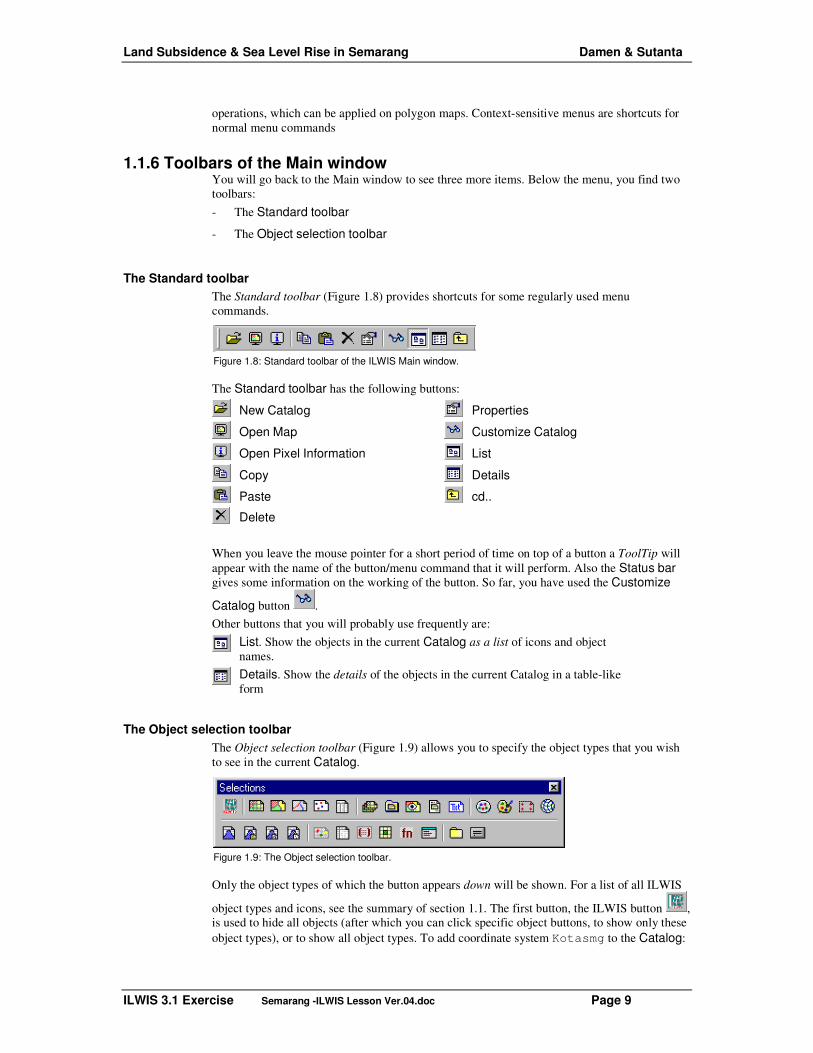
The Standard toolbar The Standard toolbar (Figure 1.8) provides shortcuts for some regularly used menu commands.
Figure 1.8: Standard toolbar of the ILWIS Main window.
The Standard toolbar has the following buttons:
New Catalog Properties
Open Map Customize Catalog
Open Pixel Information List
Copy Details
Paste cd..
Delete
When you leave the mouse pointer for a short period of time on top of a button a ToolTip will appear with the name of the button/menu command that it will perform. Also the Status bar gives some information on the working of the button. So far, you have used the Customize
Catalog button . Other buttons that you will probably use frequently are:
List. Show the objects in the current Catalog as a list of icons and object names.
Details. Show the details of the objects in the current Catalog in a table-like form
The Object selection toolbar The Object selection toolbar (Figure 1.9) allows you to specify the object types that you wish to see in the current Catalog.
Figure 1.9: The Object selection toolbar.
Only the object types of which the button appears down will be shown. For a list of all ILWIS
object types and icons, see the summary of section 1.1. The first button, the ILWIS button , is used to hide all objects (after which you can click specific object buttons, to show only these object types), or to show all object types. To add coordinate system Kotasmg to the Catalog:

Land Subsidence & Sea Level Rise in Semarang Damen & Sutanta
ILWIS 3.1 Exercise Semarang -ILWIS Lesson Ver.04.doc Page 10
��
• Press the Coordinate Systems button in the Object selection toolbar. Coordinate system Kotasmg is now added to the Catalog.
To hide the coordinate system again;
��
• Click the Coordinate Systems button again.
1.1.7 The Command line The last item we will discuss now is the Command line (Figure 1.10).
Figure 1.10: The ILWIS Command line.
You can use the Command line to type MapCalc formulas when you want to calculate with raster maps, but also other operations can be performed by typing an expression on the Command line.. The Command line has a History. You can use: - the Arrow Up key of your keyboard to retrieve previously used expressions and
commands;
- the Arrow Down key to scroll forwards again, and
- the Arrow Down button at the right hand side of the Command line to open a list of previously used commands and expressions.
1.1.8 Getting help
��
• Open the Help menu.
The ILWIS Help allows you to obtain information from any point within the program. The Help menu differs per window. In the Main window the Help menu has many options; we will explain a few of them now:
− Help on this Window. You obtain help on the current window. Depending on the window from which you select this help option, you can get help on the Main window, the map window, the table window, the pixel information window, etc.
− Related Topics. When this menu option is selected a dialog box appears with a list of topics that are related to the current window.
− Contents. Displays the Help Contents. By clicking the links in the table of contents you can go to any help topic you like.
− Index. The Index page of the ILWIS Help is displayed. Type a keyword or click any keyword in the list on which you wish to get help.
− Search. The ILWIS Help viewer is opened with the Search tab selected. Type some characters of the keyword or phrase on which you want to obtain help and press Enter ↵ or click the List Topics button to get a list of topics. In the Select topic list box select the topic you want to display and click the Display button or press Enter ↵.

Land Subsidence & Sea Level Rise in Semarang Damen & Sutanta
ILWIS 3.1 Exercise Semarang -ILWIS Lesson Ver.04.doc Page 11
− Basic Concepts. Gives an overview of the basic concepts of ILWIS. These concepts will be treated in chapter 2 of the User’s Guide.
��
• Select from the Help menu the command Help on this Window. The ILWIS Help viewer (Figure 1.11) is opened and the help topic Main Window, Contents is shown.
• Click the hyperlink Introduction. The ILWIS Help viewer refreshes and displays the topic Main window: Introduction, in which all parts of the Main window are explained.
• Click any of the links. Another topic appears explaining you more.
Figure 1.11: The ILWIS HTML Help viewer.
The ILWIS HTML Help viewer (Figure 1.11) has three parts:
− a Topic pane that shows the topic the user has selected;
− a Navigation pane with 4 tabs: a Contents tab, an Index tab, a full-text Search tab, and a Favorite tab;
− a Toolbar which allows users to Show or Hide the Navigation pane, to move Forward to the next topic or Back to the previous topic, to go to the Home/Contents Page topic, and to adapt the Font size, to Print topics and to change the Options.
To find a Help topic, click one of the following tabs in the help window:
− To browse through topics by category, click the Contents tab.
− To see a list of index entries, click the Index tab and then either type a word or scroll through the list.
− To search for words or phrases that may be contained in a help topic, click the Search tab. In the left of the Help window, click the topic, index entry, or phrase to display the corresponding topic in the Topic pane.
Land Subsidence & Sea Level Rise in Semarang Damen & Sutanta
ILWIS 3.1 Exercise Semarang -ILWIS Lesson Ver.04.doc Page 12
��
• Use the browse buttons Back and Forward to go page by page through the Help.
• Practice a bit more with the ILWIS Help. When you have finished, close the Help window by double clicking the Control-menu icon in the Title bar of the Help viewer.
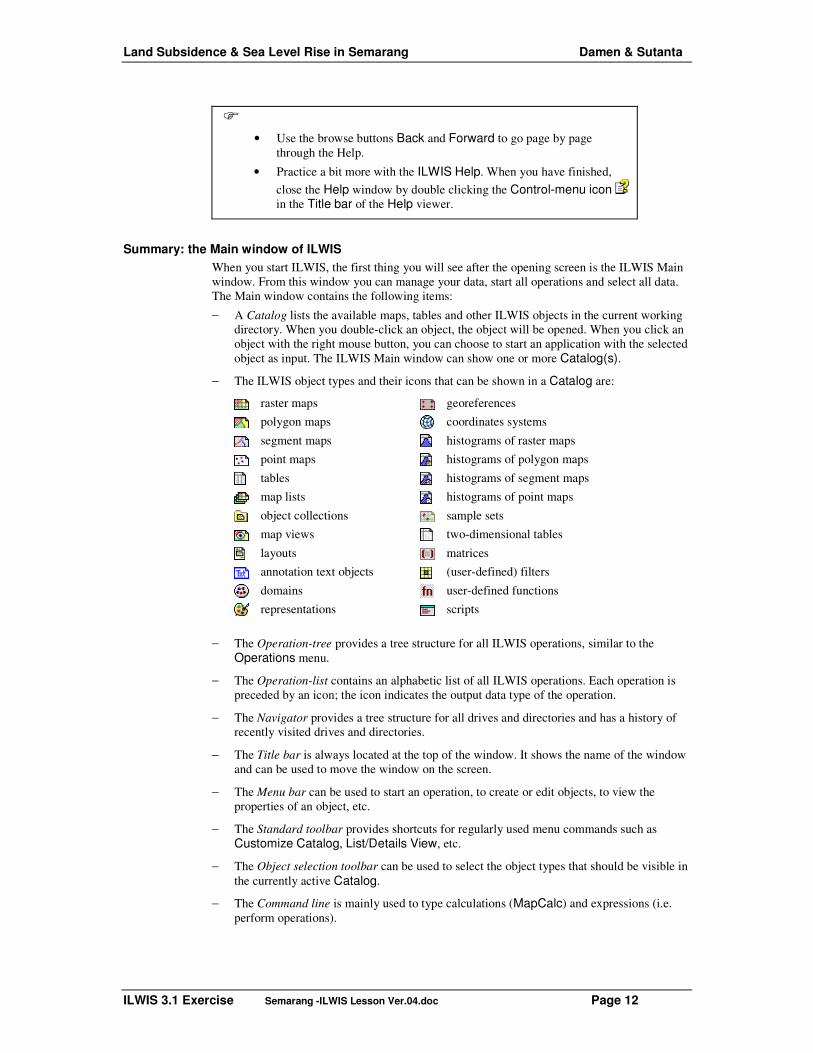
Summary: the Main window of ILWIS When you start ILWIS, the first thing you will see after the opening screen is the ILWIS Main window. From this window you can manage your data, start all operations and select all data. The Main window contains the following items:
− A Catalog lists the available maps, tables and other ILWIS objects in the current working directory. When you double-click an object, the object will be opened. When you click an object with the right mouse button, you can choose to start an application with the selected object as input. The ILWIS Main window can show one or more Catalog(s).
− The ILWIS object types and their icons that can be shown in a Catalog are:
raster maps georeferences
polygon maps coordinates systems
segment maps histograms of raster maps
point maps histograms of polygon maps
tables histograms of segment maps
map lists histograms of point maps
object collections sample sets
map views two-dimensional tables
layouts matrices
annotation text objects (user-defined) filters
domains user-defined functions
representations scripts
− The Operation-tree provides a tree structure for all ILWIS operations, similar to the
Operations menu.
− The Operation-list contains an alphabetic list of all ILWIS operations. Each operation is preceded by an icon; the icon indicates the output data type of the operation.
− The Navigator provides a tree structure for all drives and directories and has a history of recently visited drives and directories.
− The Title bar is always located at the top of the window. It shows the name of the window and can be used to move the window on the screen.
− The Menu bar can be used to start an operation, to create or edit objects, to view the properties of an object, etc.
− The Standard toolbar provides shortcuts for regularly used menu commands such as Customize Catalog, List/Details View, etc.
− The Object selection toolbar can be used to select the object types that should be visible in the currently active Catalog.
− The Command line is mainly used to type calculations (MapCalc) and expressions (i.e. perform operations).

Land Subsidence & Sea Level Rise in Semarang Damen & Sutanta
ILWIS 3.1 Exercise Semarang -ILWIS Lesson Ver.04.doc Page 13
− The Status bar gives short information on the item on which the mouse pointer is located: a menu command, a button in the Toolbar, an object in the Catalog, an operation in the Operation-list or the Operation-tree, etc.
− The ILWIS Help allows you to obtain help information from any point within the program. The ILWIS Help viewer has a Topic pane, a Navigation pane and a Toolbar.
1.2 Displaying geographic data
Geographic data are organized in a geographic database. This database can be considered as a collection of spatially referenced data that acts as a model of reality. There are two important components of geographic data (Figure 1.2.1): the geographic position and the attributes, entities or properties. In other words, spatial data (where is it?) and attribute data (what is it?) are distinguished. In the example of Figure 1.2.1, you can see that we have a (very simplified) map on one side and a table on the other. Maps are considered spatial data, since the information they contain is directly related to certain locations on the earth’s surface. The location of the units A, F and G are specified with respect to their X and Y coordinates. Tables, on the other hand, do not contain direct information on a location. They contain descriptive information (in this case the names of the land use types and the value of the land in monetary units). If we would only have the table, the data would not be useful, since we don’t know where the units are located. If we would only have the map, we still don’t know anything about the units. In a Geographic Information System (GIS) like ILWIS, the link between spatial and attribute data is the key to get real information. Only by combining spatial and attribute data we can get answers to questions such as: Where are the land use units with a value more than 250?
Figure 1.2.1: Spatial and non-spatial data in ILWIS.
In the following pages we will show you how to display spatial data and attribute data in ILWIS. We will introduce you to the map window and you will practice displaying a map. The map to be displayed is the polygon map Administration that shows the different administrative units (‘desa”) in Semarang, Indonesia. This map was digitized from a paper map. A polygon map is a vector data object containing closed areas including the boundaries making up the areas, which in this case represent the administrative units.
ILWIS dialog boxes
��
• Press the polygon map button in the Object selection toolbar to show the polygon maps again and double-click the polygon map Administration in the Catalog. The Display Options - Polygon Map dialog box appears (see Figure 1.2.3).

Land Subsidence & Sea Level Rise in Semarang Damen & Sutanta
ILWIS 3.1 Exercise Semarang -ILWIS Lesson Ver.04.doc Page 14
Figure 1.2.3: Example of a Display Options - Polygon Map dialog box.
A dialog box allows the user to enter the information required by ILWIS to carry out an operation. Dialog boxes differ depending on the application you are performing. The dialog box, which is displayed now, is used to specify how you want to display a polygon map. In general, an ILWIS dialog box can have features such as: Title bar. Shows the name of the dialog box and can be used to move the dialog box on the screen. In this case the title is: Display Options - Polygon Map.
Text box. A small box, which can be used for typing text or values. The dialog box shown on your screen contains a Text box in which you can specify the Boundary Width of the land use units lines.
Drop-down list box. A small box with an Arrow Down button , which allows you to select items. A list, including the available data, will be displayed when the arrow button or list box is
clicked. The button on the right hand side is the create button. The Create button can be used to create an object when the list excludes a proper object. When you click the Create button, the program proceeds to a new dialog box. The dialog box in Figure 1.13 contains two list boxes: one in which you can specify the color of the boundary lines of the land use units (Boundary Color), and another (Representation) in which you can indicate the color of the units themselves. These colors are stored in an object called representation (see section 2.4).
Check box. This is a small square in the dialog box, which allows you to select or clear an option. The Display Options – Polygon Map dialog box has five check boxes. When you select the Info check box, you will be able to read information about the meaning of the land use units, once the map is displayed. The second box Scale Limits allows you to define the scale limits of the map. The third check box Mask allows you to selectively display some land use types. If the fourth box, Boundaries Only is selected, only the boundaries of the land use units will be shown. Finally, the fifth box, Attribute, can be selected if you want to display an attribute value from a table connected to the map, instead of the land use units themselves.
Command buttons are used to initiate an action. The OK, Cancel, and Help are common command buttons.

Land Subsidence & Sea Level Rise in Semarang Damen & Sutanta
ILWIS 3.1 Exercise Semarang -ILWIS Lesson Ver.04.doc Page 15
OK button: whenever you click the OK button (or press Enter ↵ on the keyboard) the dialog box is closed and the action will be executed.
Cancel button: when you click the Cancel button (or press Esc on the keyboard) the dialog box is closed and the action is canceled.
Help button: when you click the Help button (or press F1 on the keyboard) context-sensitive help information will be displayed. Context-sensitive help means help dealing with the specific dialog box.
Option buttons. Option buttons can be seen as circles and represent a group of mutually
exclusive options. The selected option button contains a black dot. You can select one option at a time. Selecting another Option button, clears the other. As you can see, ILWIS gives suggestions for options in the dialog box, which are called the defaults.
! To select a check box or an Option button click the check box or press the Spacebar. If the name of the option or check box has an underlined letter, you can select the Option button or check box by pressing and holding down the Alt-key while typing the underlined letter.
��
• Select the check box Boundaries Only. Now you will see that the contents of the whole dialog box changes. If you only want to show the boundary lines of the units, no input is needed anymore on how you want to display the units themselves. The content of the dialog box depends on the input of the user. That is why we call it context-sensitive.
• Select the drop-down list box Boundary Color. You will see a list with all different types of colors that you can select.
• Practice some more with the different options in the dialog box. After that, change all options again so that they are the same as in Figure 1.13. Then confirm your input by clicking the OK button or by pressing Enter ↵.
! You can move through the various options within a dialog box by using the Tab-key or the Shift+Tab-keys on the keyboard.
A map window The polygon map Administration is displayed in a map window (see Figure 1.2.4). All maps in ILWIS are displayed in a map window. The map window has many similar features as the Main window of ILWIS, which we have seen before. It consists by default of a: Title bar: located at the top of the map window. The Title bar shows the name of the window and can be used to move the map window. Menu bar: located just below the Title bar. A map window has 5 menus: File, Edit, Layers, Options and Help. Toolbar: located just below the Menu bar. The Toolbar provides shortcuts for some regularly used Menu commands. The Toolbar of the map window has the following buttons:
Entire Map Zoom Out
Redraw Normal

Land Subsidence & Sea Level Rise in Semarang Damen & Sutanta
ILWIS 3.1 Exercise Semarang -ILWIS Lesson Ver.04.doc Page 16
Measure Distance Add Layer
Pan Remove Layer
Zoom In Save View
Scale box: Text box in which you can type the scale on which the map(s) should be displayed. Layer Management pane: The left central part of the map window displays the layers (maps) that are added to the map window and the legend of each map. In the Layer Management pane, you can for instance change the order of the layers that are displayed. The Layer Management pane will be extensively treated in the next chapter. Map viewer: The right central part of the map window where the maps are displayed. Status bar: located at the bottom of the window. The Status bar displays coordinates in meters and/or geographic coordinates.
C o n t ro l m e n u ic o n M e n u b a r
T o o lb a r
T it le b a r S c a le b o x
S ta tu s b a r S c ro ll b a r M a p v ie w e r Figure 1.2.4: An ILWIS Map window.
The map window can be moved, like all windows, by activating it and dragging it to another position. The size of the map window can be changed in several ways.
��
• Move with the mouse pointer to a border or to a corner of the map window. The mouse pointer changes into a two-headed arrow.
• Drag (press the left mouse button and hold it down) the border or corner until the window has the size you want and release the left mouse button. The map window has been resized.
• Maximize the map window by clicking the Maximize button in the upper right corner of the window.
Land Subsidence & Sea Level Rise in Semarang Damen & Sutanta
ILWIS 3.1 Exercise Semarang -ILWIS Lesson Ver.04.doc Page 17
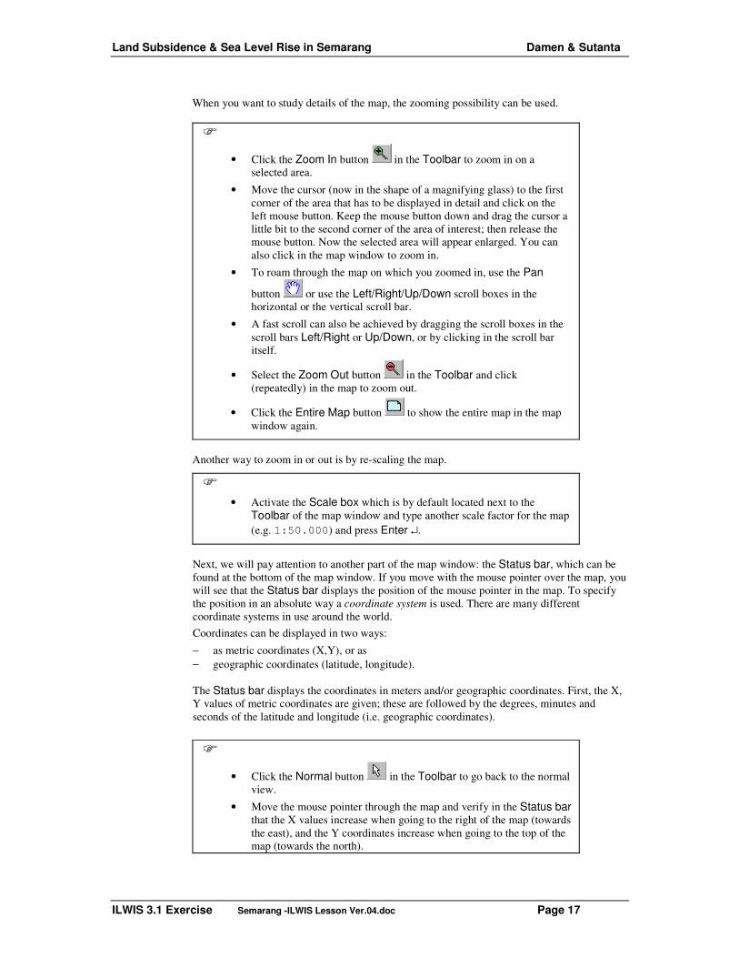
When you want to study details of the map, the zooming possibility can be used.
��
• Click the Zoom In button in the Toolbar to zoom in on a selected area.
• Move the cursor (now in the shape of a magnifying glass) to the first corner of the area that has to be displayed in detail and click on the left mouse button. Keep the mouse button down and drag the cursor a little bit to the second corner of the area of interest; then release the mouse button. Now the selected area will appear enlarged. You can also click in the map window to zoom in.
• To roam through the map on which you zoomed in, use the Pan
button or use the Left/Right/Up/Down scroll boxes in the horizontal or the vertical scroll bar.
• A fast scroll can also be achieved by dragging the scroll boxes in the scroll bars Left/Right or Up/Down, or by clicking in the scroll bar itself.
• Select the Zoom Out button in the Toolbar and click (repeatedly) in the map to zoom out.
• Click the Entire Map button to show the entire map in the map window again.
Another way to zoom in or out is by re-scaling the map.
��
• Activate the Scale box which is by default located next to the Toolbar of the map window and type another scale factor for the map (e.g. 1:50.000) and press Enter ↵.
Next, we will pay attention to another part of the map window: the Status bar, which can be found at the bottom of the map window. If you move with the mouse pointer over the map, you will see that the Status bar displays the position of the mouse pointer in the map. To specify the position in an absolute way a coordinate system is used. There are many different coordinate systems in use around the world. Coordinates can be displayed in two ways:
− as metric coordinates (X,Y), or as − geographic coordinates (latitude, longitude).
The Status bar displays the coordinates in meters and/or geographic coordinates. First, the X, Y values of metric coordinates are given; these are followed by the degrees, minutes and seconds of the latitude and longitude (i.e. geographic coordinates).
��
• Click the Normal button in the Toolbar to go back to the normal view.
• Move the mouse pointer through the map and verify in the Status bar that the X values increase when going to the right of the map (towards the east), and the Y coordinates increase when going to the top of the map (towards the north).

Land Subsidence & Sea Level Rise in Semarang Damen & Sutanta
ILWIS 3.1 Exercise Semarang -ILWIS Lesson Ver.04.doc Page 18
• Try to locate the mouse pointer on the following X and Y coordinates: X=432892, and Y=9232182, and find the corresponding latitude and longitude.
With the Measure Distance button it is easy to measure the distances and the angle between two points.
��
• Click the Measure Distance button in the Toolbar of the map window, or choose the Measure Distance command from the Options menu.
• Locate the mouse pointer somewhere in the map, and press the left mouse button. Move to another point, while keeping the left mouse button pressed. When you release the mouse button a message box appears.
The Distance message box will state: From: the XY-coordinate of the point where you started measuring;
To: the XY-coordinate of the point where you ended measuring;
Distance on map: the distance in meters between starting point and end point calculated in a plane;
Azimuth on map: the angle in degrees between starting point and end point related to the grid north;
Ellipsoidal Distance: the distance between starting point and end point calculated over the ellipsoid;
Ellipsoidal Azimuth: the angle in degrees between starting point and end point related to the true North, i.e. direction related to the meridians (as visible in the graticule) of your projection.
Scale Factor: direct indicator of scale distortion, i.e. the ratio between distance on the map/true distance.
��
• Click OK in the Distance box and click the Normal button in the Toolbar to go back to the normal view.
The contents of the map: domain You can obtain information on the map contents simply by pressing the left mouse button on any of the colored units in the map.
��
• Press the left mouse button on different units in the map to find out what they represent.
• Find the land use class around the location: X=436641 and Y=9230705.
Land Subsidence & Sea Level Rise in Semarang Damen & Sutanta
ILWIS 3.1 Exercise Semarang -ILWIS Lesson Ver.04.doc Page 19
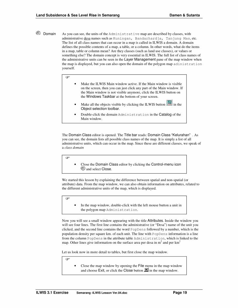
Domain As you can see, the units of the Administrative map are described by classes, with administrative desa names such as Kuningan, Bandarhardja, Tanjung Mas, etc. The list of all class names that can occur in a map is called in ILWIS a domain. A domain defines the possible contents of a map, a table, or a column. In other words, what do the items in a map, table or column mean? Are they classes (such as land use classes), or values or something else? The domain concept is very essential in ILWIS. The full list of class names of the administrative units can be seen in the Layer Management pane of the map window when the map is displayed, but you can also open the domain of the polygon map adinistration yourself.
��
• Make the ILWIS Main window active. If the Main window is visible on the screen, then you can just click any part of the Main window. If the Main window is not visible anymore, click the ILWIS button on the Windows Taskbar at the bottom of your screen.
• Make all the objects visible by clicking the ILWIS button in the Object selection toolbar.
• Double-click the domain Administration in the Catalog of the Main window.
The Domain Class editor is opened. The Title bar reads: Domain Class “Kelurahan” . As you can see, the domain lists all possible class names of the map. It is simply a list of all administrative units, which can occur in the map. Since these are different classes, we speak of a class domain
��
• Close the Domain Class editor by clicking the Control-menu icon and select Close.
We started this lesson by explaining the difference between spatial and non-spatial (or attribute) data. From the map window, we can also obtain information on attributes, related to the different administrative units of the map, which is displayed.
��
• In the map window, double-click with the left mouse button a unit in the polygon map Administration.
Now you will see a small window appearing with the title Attributes. Inside the window you will see four lines. The first line contains the administrative (or “Desa”) name of the unit you clicked, and the second line contains the word PopDens followed by a number, which is the population density per square km. of each unit. The line with PopDens information is a line from the column PopDens in the attribute table Administration, which is linked to the map. Other lines give information on the surface area per desa in m2 and per km2
Let us look now in more detail to tables, but first close the map window.
��
• Close the map window by opening the File menu in the map window and choose Exit, or click the Close button in the map window.
Land Subsidence & Sea Level Rise in Semarang Damen & Sutanta
ILWIS 3.1 Exercise Semarang -ILWIS Lesson Ver.04.doc Page 20
A table window
Table We will finish this chapter by showing you how to display attribute data.
��
• In the Catalog, double-click the table Administration.
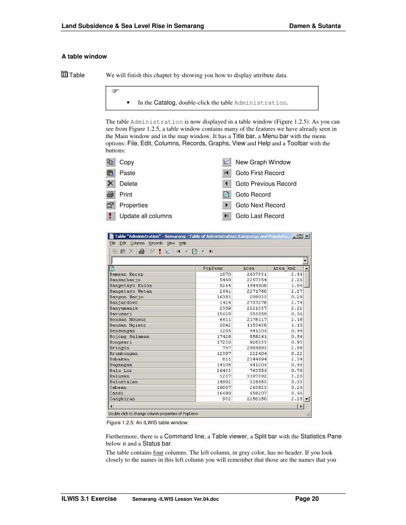
The table Administration is now displayed in a table window (Figure 1.2.5). As you can see from Figure 1.2.5, a table window contains many of the features we have already seen in the Main window and in the map window. It has a Title bar, a Menu bar with the menu options: File, Edit, Columns, Records, Graphs, View and Help and a Toolbar with the buttons:
Copy New Graph Window
Paste Goto First Record
Delete Goto Previous Record
Print Goto Record
Properties Goto Next Record
Update all columns Goto Last Record
Figure 1.2.5: An ILWIS table window.
Furthermore, there is a Command line, a Table viewer, a Split bar with the Statistics Pane below it and a Status bar. The table contains four columns. The left column, in gray color, has no header. If you look closely to the names in this left column you will remember that those are the names that you

Land Subsidence & Sea Level Rise in Semarang Damen & Sutanta
ILWIS 3.1 Exercise Semarang -ILWIS Lesson Ver.04.doc Page 21
have seen also in the map Administration. This is again the domain; a domain can thus define the contents of a map, but also the contents of a table. Next to the left gray column containing the domain items, the table has one column, called PopDens. This column is an attribute column that contains the population density of the administrative units. As you can see, this column contains values. Next to this column you see the column Area (values in square meter) and Area_km2.
��
• Double-click the Column header with the name PopDens on it. The Column Properties dialog box (Figure 1.16) appears.
Figure 1.16: Example of a Column Properties dialog box.
This dialog box contains information on column PopDens. The dialog box shows for instance the domain of column PopDens: Default Value Domain. The next line gives the Value Range of column PopDens: between 0 and 10000. The actual values in the column are also shown: Minimum: 0, Maximum: 32163.
��
• Click the Cancel button to close the Column Properties dialog box.
Information on the Minimum (Min) and Maximum (Max) values in the column, together with the Average (Avg), Standard Deviation (StD) and Sum of the column, is visible in the Statistics Pane in the lower part of table Administration. By clicking the Column option in the dialog box, you can select the column which you wish to sort. The record order of the table will change as well.
Summary: displaying maps and tables In this section you have learned:
− How to use dialog boxes: How to enter parameters to define the way in which a map is displayed.
Land Subsidence & Sea Level Rise in Semarang Damen & Sutanta
ILWIS 3.1 Exercise Semarang -ILWIS Lesson Ver.04.doc Page 22
− The basics of a map window: How to open a map; the different components of a map window: Title bar, Menu bar, Toolbar, Map viewer, Layer Management Pane, Status bar; to resize a map window; to zoom in and to zoom out; to read the coordinates of a map (coordinate system); to know the contents of a map (domain).
− The basics of a table window: How to open a table; the different components of a table window: Title bar, Menu bar, Toolbar, Command line, Table viewer, Split bar, Statistics Pane, Status bar; the fact that contents of a table are defined by the domain of the table; the fact that columns also have a domain. The display of an entire table (i.e. Table View), or only the contents of a certain record (i.e. Record View); to sort a table.
Land Subsidence & Sea Level Rise in Semarang Damen & Sutanta
ILWIS 3.1 Exercise Semarang -ILWIS Lesson Ver.04.doc Page 23
LESSON 2
Crude Assessment of Coastal Flood Hazard Zones using NOAA GLOBEDEM data of Java, Indonesia
Objective
To display, analyze and quantify coastal areas in Indonesia with a low elevation (less than 2m), which are vulnerable to enhanced sea level rise, using downloaded GLOBEDEM data Available data Indonesia Raster Map with a pixel size of approx. 900 m and a vertical resolution of
1m. The DEM has been downloaded from the NOAA GLOBEDEM website: http://www.ngdc.noaa.gov/seg/topo/globe.shtml
2.1. Display and analysis of GLOBEDEM data
The map Indonesia can be displayed as follows:
��
• Left mouse-click the raster map icon Indonesia in the ILWIS Catalog. Use the default values in the Display Options – Raster Map window by selecting OK.
Remark: the map has been given the Color Look-Up table Indonesia
• Left mouse-click in the image to see the elevation in meters. Zoom in to certain areas of interest, in particular those along the coastline.
! Try to find areas / cities you know. Where is Semarang located?
• To see the properties of the map, select: File, Properties, Map Indonesia. In the Properties of Raster map window you can see that that it is a value map with a range between 0 and over 5179 meters with a (vertical) precision of ~ 1.0 meter.
Next, the map Indonesia should be analyzed for areas vulnerable to coastal flooding. This is for instance the coastal zone at an elevation of four meters or less above mean sea level.

Land Subsidence & Sea Level Rise in Semarang Damen & Sutanta
ILWIS 3.1 Exercise Semarang -ILWIS Lesson Ver.04.doc Page 24
For this, first a new map IndonCoast has to be made in which only elevations are given from 0 --> 2.0 meter. After this the quantification of the areas vulnerable to enhanced sea level rise is explained by analyzing the histogram of the map.
��
• To make a new map with the name IndonCoast, in which only elevations are given of 0 --> 2.0 meter, you have to type the following Map Calculation formula in the Command Line:
IndonCoast:=iff(Indonesia<=2,Indonesia,?)
Meaning: If the map Indonesia has an elevation of 2.0 meter or less, keep the map Indonesia as it is, and make all other values in the new map (also the land) undefined = ?.
• Check the correct typing of the MapCalc formula and press Enter. In the Raster Map Definition window are given the Value Range, Precision and Domain of the new map. Press: Show.
• Study the new map IndonCoast by browsing through it with the mouse.
• Select the IndonCoast histogram icon from the ILWIS Catalog. Remark: The histogram has been made ‘automatically’ when the map was displayed before.
• Study the values in the IndonCoast histogram. In the Npix column the number of pixels are given per elevation class: 1or 2 meter above the sea level !
Question: How much square kilometer is the hazard zone for an enhanced sea level rise of 1 meter? Answer: ………………………………………………………
2.2. Downloading of other GLOBEDEM data from the internet
(optional exercise) For this exercise you need enough time for downloading and a relatively fast internet connection !
The instructions will guide you through the process of downloading GLOBEDEM data from the NOAA National Data Center (NGDC) website and import into ILWIS 3.1. The cell size of the D.E.M. data is a little bit more than 900 meter and the vertical accuracy is approximately 1 meter.
The following steps have to be followed: a. Downloading of the data in xxx.bin format (2 bytes per pixel) b. Importing of the downloaded file into ILWIS 3.1 as general raster data

Land Subsidence & Sea Level Rise in Semarang Damen & Sutanta
ILWIS 3.1 Exercise Semarang -ILWIS Lesson Ver.04.doc Page 25
Downloading of the data in xxx.bin format (2 bytes per pixel):
��
• Open the GLOBE site of the NOAA National Data Center Home Page: http://www.ngdc.noaa.gov/seg/topo/globeget.shtml
• In the ‘Global Land One-km Base Elevation Project’ window
select: Get Data • In the 'Get GLOBE Data' window select: Select your own area
• In the 'GLOBE: Customize Your Data Selection’ window select: ���� Map-Based (uses Java script)
��In the global map: window of your subset (zoom in, if necessary)
��Export type: FreeFormND ��Data type: int16 ��File format: PC binary ��Compression option: Individual files ��Transfer option: FTP ��Enter: File name for your data selection (no more than 8
characters) ��Enter: Title of your data selection ��Enter: your Email address ��Press: Update this form ��Read the text in the blue box and write down:
Number of rows Number of Columns Size (Bytes)
Remark: Do not make the file size larger than approx. 3 Mb. If so, make your subset smaller. This will speed up the downloading process!!
��Press: Get Data
• In the 'GLOBE - Data is being processed' window Wait two to three minutes until the processing is being completed. Pages are being refreshed every 60 seconds
• In the 'GLOBE - Processing Complete!' window Select your filename with the *.bin extension by a right-mouse click and "Save Target As…" in a directory of your choice. Now your file is being copied from the NGDC -FTP server to your machine.
��Also save the file with the *.hdr extension. This is a text file with the coordinates, grid size in degrees and other image properties.
��Wait until download of the files is complete. After this, close the window.

Land Subsidence & Sea Level Rise in Semarang Damen & Sutanta
ILWIS 3.1 Exercise Semarang -ILWIS Lesson Ver.04.doc Page 26
Importing of GLOBEDEM xxx.bin data file into ILWIS 3.1 :
�� • Start ILWIS and move to the folder with the downloaded xxx.bin file
• Open the GLOBE site of the NOAA National Data Center Home
• Select: File, Import, General Raster… ��Select the downloaded file ( xxx.bin ) ��Enter for Output File name: a new name (or leave it as it is)
Press: OK
• In the 'Import Raster' window, select: ��Header Size: 0 ��Number of Bands: 1 ��Number of Columns: the number written down in the
above table ��Pixel structure: Integer numbers ��Numbers of bytes per pixel: 2 ��File Structure: Band Interleaved ��Copy: Covert to ILWIS data format ��Enter: Output name (a new name, or leave it as it is)
Press: OK
• Open the newly created raster map. Check the elevation in meters per pixel. Unfortunately the maps have no geographical coordinates. This, you have to do by yourself.

Land Subsidence & Sea Level Rise in Semarang Damen & Sutanta
ILWIS 3.1 Exercise Semarang -ILWIS Lesson Ver.04.doc Page 27
LESSON 3
Display and analysis of satellite images and the coastline of Semarang Landsat Enhanced Thematic Mapper, ASTER-1B and ‘old’ Landsat Multi Spectral Scanner (MSS) data
Objective To display and analyze the available images andto overlay them with some digitized coastlines of the Semarang area (1871 and 1992..
3.1 Making of color-composites Color composites are formed by displaying the different channels or bands of multi-spectral images on the red, green and blue (RGB) guns of the computer's monitor. Initial inspection of such composite images, which for appropriate sensors can look very similar to color aerial photographs or infra-red photographs, may provide a much better idea of what is in the image than just looking at individual bands in isolation. The first task in this exercise is to make a true color composite and a false color composite which will give you a color photograph like view of the image from space, making it fairly clear what is land and what is sea. The second task is to explore these color composites to find out more about the spectral signatures of major features of the images.
Image files used for this exercise:
File name File contents MSS72b1,…b2,…b3,…b4
Raster map of Landsat MSS image of 23 September 1972, bands 1 � 4. Resolution of all bands: 79m.
ETM01b1,…b2,…b3,…b4, …b5,…b8
Raster map of the Enhanced Thematic-Mapper image of 2th August 2001, bands 1 �5 and band 8. Resolution bands 1 � 5 is 30m and of band 8: 15 m.
ASTER01b1,…b2,…b3 Raster Map of ASTER-1B image of 16 February 2001, bands 1 � 3, with a resolution of 15m.
Coastlines Segment map of the coastline, digitized from topographical maps of 1871 and 1992
Display of color-composites of Landsat ETM+ and MSS images
If you have browsed to the correct directory you will see in the Catalog of the Main Window the list of individual image bands, displayed with a raster icon.
��
• Double mouse-click ETM01b5 image. Accept the default settings in the “Display Options- Raster Map” window by selecting OK. Browse through the image with the mouse pointer and try to recognize certain surface features; for instance the difference between the land and sea area, the infra-structure of Semarang, etc. Zoom in at certain areas.
Land Subsidence & Sea Level Rise in Semarang Damen & Sutanta
ILWIS 3.1 Exercise Semarang -ILWIS Lesson Ver.04.doc Page 28
• Do the same for ETM01b8. Compare the result in screen windows next to each other. As you will see, the image ETM01b5 has a lower spatial resolution (30 m pixel size) than the panchromatic ETM01b8 (15 m pixel size).
• Make a color composite of the Enhanced Thematic Mapper bands 4, 5 & 3 for red, green and blue. Save the result as ETM01b453
To do this select from the Menu Bar: ��Operations, Image Processing, Color-Composite…
Select in the Colour-Composite window the following bands: Red – Green – Blue: ETM01b4–ETM01b5–ETM01b3
��Type for Output Raster map: ETM01b453 ��Keep the defaults and Press: Show
• Study the colors of the image, and zoom-in at selected sites.
• Make color-composites with different band combinations as well.
Diplay of an ‘old ‘ Landsat Multi Spectral image of 1972, with a pixel size of 79m.
��
• Double mouse-click MSS72b1 image. Do the same for the other bands.
• Make a color composite of the Landsat MSS using bands 1, 2 and 4 for red, green and blue. Save the result as MSS01b124
Comparing the coastline of 1871 with the coastline during image acquisition
The coastline of Semarang and surroundings, as can be seen on the color-composite of the Enhanced Thematic Mapper Image and the ASTER image, can be compared with the historic coastline, digitized from a topographical map of 1871
��
• First display one of the ETM color-composites images of your own choice.
• Add the data layer Coastline by selecting from the Map window: Layers, Add Layer…
• In the Add Data Layer window select the segment map: Coastlines ,OK. In the Display Options-Segment Map window select all defaults by also OK.
• Zoom in at the coast and compare the historical coastline(1871 – orange color) with the more recent one (1992 – red color)
Image enhancement by supervised stretching / histogram equalization of ASTER images
If you display one of the bands of the ASTER image in default mode, you will see that it looks quite ‘dark’ compared to the individual bands of Thematic Mapper. Image enhancement by supervised linear stretching and histogram equalization will be necessary. For this, first the minimum and maximum DN values of the image histogram have to be determined, between which the image should be stretched for a good result.

Land Subsidence & Sea Level Rise in Semarang Damen & Sutanta
ILWIS 3.1 Exercise Semarang -ILWIS Lesson Ver.04.doc Page 29
��
• First make a histogram by selecting from the Catalog of the Main Window: Operations, Statistics, Histogram.
• Select in the Calculate Histogram window the map ASTER01b1 and press: Show.
• Study the minimum and maximum DN values of the histogram; for instance from the first or second ‘peak’ in the number of pixels, which represent ‘land’ resp. ‘sea’ in this image band. Write down the values per image band in the table below.
• Display the image ASTER01b1 again with the new Min. and Max. values (for instance ‘sea’ or ‘land’). To do this double mouse-click the map ASTER01b1, and in the Display Options – Raster Map window fill in your own values under Stretch
• Repeat the above procedure with other bands from your own choice.
Band 1 Band 2 Band 3
Min. DN
Max. DN
Now make new color-composites using the minimum and maximum DN values found above.
��
• Select from the Catalog of the Main window: Operations, Image Processing, Color-Composite…
• In the Color-Composite window: ��Clear the check box: Percentage ��Select in the Drop down list box of the image bands the Red-,
Green-, and Blue- bands of your own choice ��Type the minimum and maximum DN values for the stretching of
the individual image bands (your own, new values) ��Use both the options Histogram Equalization and Linear
Stretching • Assess the result, for instanceby comparing them with the ETM
images

Land Subsidence & Sea Level Rise in Semarang Damen & Sutanta
ILWIS 3.1 Exercise Semarang -ILWIS Lesson Ver.04.doc Page 30
LESSON 4
Spatial Modeling of Urban Land Subsidence and Sea Level Rise using a recent DEM and benchmarks of land subsidence
Objective To model land subsidence and enhanced sea level rise for scenarios of the years 2010, 2019 and 2070, using a DEM of 1991, and a point map of the benchmarks of the subsidence rate
Data used in the exercise:
Administration Segment and polygon maps of the administrative subdivision of the city of Semarang in ‘desas’ and the population densities in a table.
Eleva01 Point map of the elevations in 2001, in the central part of Semarang in cm
Benchmarks Point map of benchmarks with a known subsidence rate in mm per year
Topo_1871, Topo_1908, Topo_1937, Topo_1992
Scanned topographical maps of the years 1871, 1908, 1937 and 1992 with a pixel resolution of 5.
ETM01b1,…b2,…b3,…b4,…b5,…b8
Raster map of the Enhanced Thematic-Mapper image of 2th August 2001, bands 1 �5 and band 8. Resolution bands 1 � 5 is 30m and of band 8: 15 m.
ASTER01b1,…b2…b3 Raster Map of ASTER-1B image of 16 February 2001, bands 1 � 3, with a resolution of 15m.
Roads Segment and polygon map of the main roads SubsMask Raster, polygon map. Mask of study area for
subsidence
Display of data layers
First we will have a look at the administrative map and table, and the point map of the elevations, from which the Digital Elevation Model has to be constructed.
��
• Select the polygon map administration. In the Display Options – Polygon Map window you keep all defaults. Select: OK.
• Double mouse-click in the administrative units (“desas”) of Semarang. An Attribute window pops-up with information on the population density in that unit( =PopDens). Note that the population density in the Java Sea is of course 0; population data of the surrounding Kabupaten is not known ( = ? ). All population data are stored in the table Administration.

Land Subsidence & Sea Level Rise in Semarang Damen & Sutanta
ILWIS 3.1 Exercise Semarang -ILWIS Lesson Ver.04.doc Page 31
To add other data layers, such as a satellite image or a topographical map, you have to display the administration map with the boundaries only.
��
• Select in the Polygon Map window: Layers, Display Options, 1 pol. Administration. In the Display Options – Polygon Map window you select the Check Box Boundaries Only. Select: OK. Now, the Administration map is displayed with boundaries only in a red color.
• In the Polygon Map window select: Layers, Add Layer. Now you can choose a map to add to the polygon map.
Add the maps one by one: Topo_1992 or Topo_1871,Topo_1908,Topo_1937 or ETM01b453, or ASTER01b321 (if you have).
Study the change of the coastline and the extension of the city, compared to the historic data.
You can use the layer management pane (left window) to hide or display maps of your own choice (find out yourself)
Remark You can add only ETM images, or ASTER images or Topo maps to the Adminstration map. This has to do with differences in the geo-reference.
The display of the point map of the elevations in meters, with mm accuracy, and the benchmarks of the land subsidence rate (cm/year), can be done as follows.
��
• Display a map, for instance a satellite image or the topographical map of 1992.
• Add as data layer the point map eleva01 and/or benchmarks. Mouse click on the points to see the values.
• Improve the display of the points by selecting: Layers, Display Options, 2pnt_eleva01.. In the Display Options – Point Map window press the Symbol button. Use the Help function for more information on the different display options.
Interpolation of the elevation points and benchmarks of land subsidence
To speed up the procedure of interpolation, only the city center of Semarang will be used as a test area. For this, a special georefer_subsidence is available with a pixel size of 30 m. To make the DEM of 2001 we will use a simple interpolation algorithm: Moving Average with Inverse Distance. In ILWIS a more advanced interpolation is well possible, for instance kriging, but that will take too much time for the exercise.
��
• In the ILWIS Menu Bar select: Operations, Interpolation, Point Interpolation, Moving Average. In the Moving Average window Select / type:
��Point Map: eleva01

Land Subsidence & Sea Level Rise in Semarang Damen & Sutanta
ILWIS 3.1 Exercise Semarang -ILWIS Lesson Ver.04.doc Page 32
��Weight Function: ���� Linear Decrease ��Weight Exponent: default value ��Limiting Distance: 1500 (value in meters) ��Output raster Map: Eleva01 (value in meters) ��Georeference: Georef_Subsidence (30 m pixels) ��Value Range: default values ��Precision: 0.01 (value in cm) ��Type for Description: Elevation 2001 in meters
Select: Show • Select all default values in the Display Options – Raster Map
window..
• Browse through the map and look at the elevation values
• Add Map layers, such as roads, waterways and administration.
To make the raster map SubsRate, in which the subsidence rate in cm per year is given, we have to interpolate the point map Benchmarks. For this, we follow basically the same interpolation procedure as for the map Eleva01 (see above). We also use Georef_Subsidence (same area as eleva01). The only difference is, that the data to be interpolated are stored in a table benchmarks, and not in a map. The second difference is the limiting distance; this is set to 15.000m, to overcome the wide spacing of the benchmark point locations.
��
• In the ILWIS Menu Bar select: Operations, Interpolation, Point Interpolation, Moving Average. In the Moving Average window Select / type:
��Point Table: Benchmark Click the small box with a + in it, in front of the map icon Benchmarks. Select: Subs_cmyr
��Weight Function: ���� Linear Decrease ��Weight Exponent: default value ��Limiting Distance: 15.000 (value in meters) ��Output raster Map: SubsRate ��Georeference: Georef_Subsidence (30 m pixels) ��Value Range: default values ��Precision: 0.01 ��Type for Description: Subsidence rate in cm /yr.
Select: Show
• Select all default values in the Display Options – Raster Map window.
• Browse through the map and look at the subsidence rate values in cm per year.
• Add Map layers, such as roads,waterways and administration.

Land Subsidence & Sea Level Rise in Semarang Damen & Sutanta
ILWIS 3.1 Exercise Semarang -ILWIS Lesson Ver.04.doc Page 33
Modelling future relative Sea Level Rise The scenarios in this exercise will produce maps with estimations of the relative sea level rises for the years 2010, 2019 and 2070. This means the sea level relative to the elevations of the land, taking into account land subsidence and enhanced sea level rise. As described by H. Sutanta et al (see Appendix 2) the prediction from the study by the Asian Development Bank (1994) is taken as a basis for the absolute Enhanced Sea Level Rise scenarios in Semarang.
For the exercise, the medium values for the years 2010, 2019 and 2070 have been selected in the calculations of future land subsidence relative to enhanced sea level rise. This means a rise of 9 cm in 2010, of 13 cm in 2019 and 45 cm in 2070. The calculation for the DTM for the year t1 (=2010, 2019 or 2070), starting at the year t0 (=2001) is (H. Sutanta, 2002):
))*(( 01101 ttSUBSRATESLRELEVAELEVA ttt −+−= Where:
ELEVAt0 = elevation at the initial condition (file: Eleva01)
ELEVAt1 = elevation at the year to be estimated (file: Eleva10, Eleva19, Eleva70) SLRt1 = sea level rise at the year to be estimated (2010, 2019 and 2070)
SUBRATE = map of the rate of land subsidence (file: SubsRate)
In ILWIS, the necessary calculations based on the above formula, can be carried out using Map Calculations, to be typed in the Command Line. The equations are the following:
Remark: the values SubsRate are divided by 100, to make units in meters
in stead of cm.
��
• To make the map Eleva10, the following Map Calculation has to be performed (type in the Command Line):
Eleva10 = Eleva01 –(0.09+9*SubsRate/100)
Accept the defaults in the Raster Map Definition window and select: Show.
• Make with Map Calculation also the maps: Eleva19 and Eleva70
• Check the result and add map layers such as Administration..
Scenario 2010 2019 2070 Low (cm) 3 6 15
Medium (cm) 9 13 45 High (cm) 15 25 90
e/100)69xSubsRat(0.45Eleva01Eleva70e/100)18xSubsRat(0.13Eleva01Eleva19/100)9xSubsRate(0.09Eleva01Eleva10
+−=+−=+−=

Land Subsidence & Sea Level Rise in Semarang Damen & Sutanta
ILWIS 3.1 Exercise Semarang -ILWIS Lesson Ver.04.doc Page 34
• As you will see did the interpolation of the points does not stop at the coastline itself. To overcome this, you have to combine the resulting maps with a mask of only the land area of 2001. This is the map SubsMask, of which the coastline is digitized from the Landsat ETM image of 2001.
• Display the map SubsMask
• To ‘take out” or mask only the land area of the created elevation maps of the years 2010, 2019 and 2070, perform the following Map Calculation:
ElevaMask10 = iff(SubsMask=”Land”, Eleva10,0) Meaning: Create a map with the name ElevaMask10 only for the areas which are “land” in the map SubsMask. Make the Sea: 0
• Accept the defaults in the Raster Map Definition window.
• Create the same way as above the maps ElevaMask19 and ElevaMask70.
• Check the results. Add data layers of your own choice.
To get a better idea, on how badly the land has subsided in 2010, 2019 and 2070 compared to 2001, we display the topographical map of 1992 and browse with Pixel Info through the map, with the elevations of the three future years displayed in the Pixel Info window.
��
• Display topomap Topo_1993 (or satellite image of 2001)
• Open Pixel Info from the Standard Toolbar
• Add the maps Eleva01, ElevaMask10, ElevaMask19, ElevaMask70, SubsRate to the Pixel Information window by selecting: File, Add Map.
• Analyze the results.
The final step is to slice the ElevaMask 10, ..19, ..70 maps in such a way, that the subsided is represented in steps with clear and nice color. For this, there is already made a domain with the steps elevation and a color look-up table with the same name. The output maps will be given the names: Elevation 2010, Elevation 2019 and Elevation 2070.
��
• Select: Slicing from the Operations List (left side of window). Type or select in the Slicing window:
��Raster Map: Elevamask10
��Output Raster Map: Elevation2010 ��Domain: Elevation ��Description: Elevation Map 2010
Select: Show • Accept the default values in the Raster Map Definition window and
Check / analyze the resulting map
• Make the same way maps Elevation2019 and Elevation2070

Land Subsidence & Sea Level Rise in Semarang Damen & Sutanta
ILWIS 3.1 Exercise Semarang -ILWIS Lesson Ver.04.doc Page 35
LESSON 5
Impact of urban flooding on population and infra-structure
Objective To calculate areas and/or numbers of elements at risk, such as main roads, industrial areas and population densities per desa, for subsidence scenarios of 2010, 2019 and 2070.
Data used in the exercise:
Administration Segment and polygon maps of the administrative subdivision of the city of Semarang in ‘kampungs’ and the population densities in a table.
Eleva01, Elevation2010, Elevation2019, Elevation2070
Elevation maps of 2001, 2010, 2019 and 2070 – Made in Lesson 4
Industrial Segment and polygon map of the industrial centers Roads Segment and polygon map of the main roads
Rasterizing of Administration, Industrial and Roads map
Before we can cross the table with the population density per “Desa”, or the Industry cq. Roads map with the elevation classes of the years 2010, 2019 and 2070, we first have to rasterize these maps, and give them all the same GeoReference. For this, we select the GeoReference of the Elevation maps, which is called: Georef_Subsidence, with a pixel size of 30m.
��
• Select: Operations, Rasterize, Polygon to Raster. In the Raster Polygon Map window you select:
��Polygon Map: Administration ��Output Raster Map: DesasAtRisk ��GeoReference: Georef_Subsidence (Pixelsize:30m) ��Description: Semarang - Population at Risk
Show.
• Repeat the above procedure, and rasterize also the maps: Industrial and Roads. Give as output names: InduAtRisk and RoadsAtRisk.
• Check the results.
Land Subsidence & Sea Level Rise in Semarang Damen & Sutanta
ILWIS 3.1 Exercise Semarang -ILWIS Lesson Ver.04.doc Page 36
Next, we can compare or ”cross” the elevation classes of 2010, 2019 and 2070 with the maps InduAtRisk and RoadsAtRisk.
��
• Select: Operations, Raster Operations, Cross. In the Cross window select:
��1st Map: InduAtRisk ��2nd Map: Elevation2010 ��Output Table:InduAtRisk2010
Show.
• In the displayed table InduAtRisk you see a column with the elevation classes of the year 2010 and the areas of the industry in that class in square meters.
• Make an extra column with the area in square hectares, in stead of square meters by the following table calculation:
Area_ha:=Area/10000 Enter
• Make the same way as above the Cross Tables: InduAtRisk2019 and InduAtRisk2070
• Make also the Cross Tables: RoadsAtRisk2010, …2019 and …2070.
Finally we compare (“cross”) the elevation maps with the PopDens per ‘Desa” in the Table Administration. Although for the whole city the population growth in the period 1994 – 1995 was 2.2% and approx 1% in the period 1997 – 1998, the population in the city center has remained more or less stable. Therefore we take for all calculations the population densities as listed in the table Administration.
��
• Select: Operations, Raster Operations, Cross. In the Cross window select:
��1st Map: Column PopDens from table: DesaAtRisk
Remark: To select the column PopDens click the small box with the cross in front of the table Administration
��2nd Map: Elevation2010 ��Output Table:PopAtRisk10
Show.
• In the displayed table PopAtRisk10 you see a column with the elevation classes of the year 2010 and the population densities in that class in the column Map1. Scroll down the table to see all values.
• To remove the many repetitions in the column Map1, we use the aggregate function and make a new table PopAtRisk2010: Selectin the Table window: Columns, Aggregation…. In the Aggregate Column window you select:
��Column: Map1 ��Function: Sum
Land Subsidence & Sea Level Rise in Semarang Damen & Sutanta
ILWIS 3.1 Exercise Semarang -ILWIS Lesson Ver.04.doc Page 37
��Group by: Elevation2010 ��Output Table: PopAtRisk2010 ��Output Column: PopDens
Press: OK
• To add the column Area to the new table PopAtRisk2010, you also aggregate the Column Area. In the Aggregate Column window select:
��Column: Area ��Function: Sum ��Group by: Elevation2010 ��Output Table: PopAtRisk2010 ��Output Column: Area
OK
• Display the table PopAtRisk2010
• To calculate the population density in square kilometer and the total population per elevation class, you do the following: First make with Table Calculation an extra column with the area in square kilometers, in stead of square meters:
Area_km2:=Area/1000000 Enter Accept the defaults in the Column Properties window.
• Next make a new column PopAtRisk by multiplying the values in the column Area_km2 with those of the column PopDens:
PopAtRisk:=Area_km2 * PopDens Enter
To draw conclusion on the amount of people at flood risk in on or more desas you can do the following:
��
• First link the attribute table PopAtRisk to the map Elevation2010 in the following way: Display the map Elevation 2010. Select: properties,and in the Properties of Raster Map window select as attribute table: PopAtRisk2010
• Add as data layer the map Administration with boundaries only.
• Open Pixel Info and add to it the maps Administration and Elevation2010.
• Browse with Pixel Info through the map and draw conclusions.
�� • Repeat the procedure as executed for 2010, also for the years 2019
and 2070

Land Subsidence & Sea Level Rise in Semarang Damen & Sutanta
ILWIS 3.1 Exercise Semarang -ILWIS Lesson Ver.04.doc Page 38
LESSON 6
Coastline Change Analysis with Historic Topographical Maps From 1871, 1908, 1937 and 1992
Objective To monitor the coastline of Semarang for the years 1871, 1908, 1937 and 1992 by usning digitized and ge-referenced topographical maps of these years.
Topographical maps have been included from a part of the Semarang coastal area of 1871, 1908, 1937 and 1992. All maps have been scanned with a resolution of 5m. In this lesson you can compare the already digitized segments maps of 1871 and 1992 with your own digitized interpretations of 1908 and 1937.
Data files used for the lesson:
Topo_1871, Topo_1908, Topo_1937, Topo_1992
Scanned topographical maps of the years 1871, 1908, 1937 and 1992 with a pixel resolution of 5.
Coastlines Digitized Coastlines based on the topographical maps of 1871 and 1992.
ETM01cc and/or ASTER01bcc
ETM01cc or ASTER 01bcc color composies previously made
Display of digitized coastlines of 1871 and 1992 on top of topographical map of 1992 and satellite image:
��
• First display the topographical maps: Topo_1871, Topo_1908, Topo_1937 and Topo_1992 next to each other, to see the differences.
• Display Topo_1992 and add the data layers Coastlines. • Analyse the areas of erosion and sedimentation and/or infra-structural
works
• Add the digitised coastlines of 1871 and 1992 also on top of a recent color-composite satellite image.
Digitize the coastlines of 1908, 1937 and of 2001 (Landsat ETM or ASTER)
�� • First display the "back-drop" image on top of which you are going to
digitise the coastline. For instance Topo_1908, Topo_1937 or

Land Subsidence & Sea Level Rise in Semarang Damen & Sutanta
ILWIS 3.1 Exercise Semarang -ILWIS Lesson Ver.04.doc Page 39
ETM01b453 (or other cc band combination).
• Select: Layers, Add layer. Add the segment data layer Coastlines.
As you see the digitized coastline of 1992 is in red and the box in which is digitized (“Mask”) has a green line color. In the legend are already the coastlines visible of all dates. But not yet digitized !!
This is because they are already included in the domain coastline, (which has been created before).
• Zoom in at details and be sure that the scanned resolution of your image is high enough to recognize all the necessary terrain features to be digitized.
• To add segments of a coastline to the map coastlines you select: Edit, Edit Layer, 2seg Coastline, OK.
• Select: Insert Mode (the icon with the pen) to insert new elements in the current map; mouse-draw carefully the first small segment. This goes best if you do it little by little while clicking regularly the left mouse button; draw the line slowly. After you have finished a segment, you double mouse-click, until an Edit window will pop-up asking for the Class Name. Select the correct Class from the drop down menu and continue digitizing, where you had ended. Segments are connected at Nodes, which are displayed as small squares.
!! Important: Always zoom-in as much as possible when you are digitizing. This will give the best results.
• If you want to connect a segment in the middle of an existing one, you mouse-click at a certain point of the line. A Segment Editor window will pop-up asking to split the segment boundary. Select: Yes At the end of the drawing of the second segment you should split again the line you are connecting it to.
• Connect more segments to the other ones.
!! Important: Always make nodes where segments are connected by splitting them. The best way is to move the cursor just before the segment you want to connect to (and not over it !). If you don't do this carefully you will be "punished" when you check the segments later.
• Segments which are not quite at the right place can be edited by the Move Points Mode. Click the icon (picture: blue and red line) and a pair of tweezers appears with which you can move the segment point by point towards its correct position.
• Segments which are completely wrong you can better delete: detailed
editing may take too long. Select the wrong segment with Select Mode (icon picture with hand) and delete it.
• To save the result select in the Segment Editor window: File, Exit Editor.
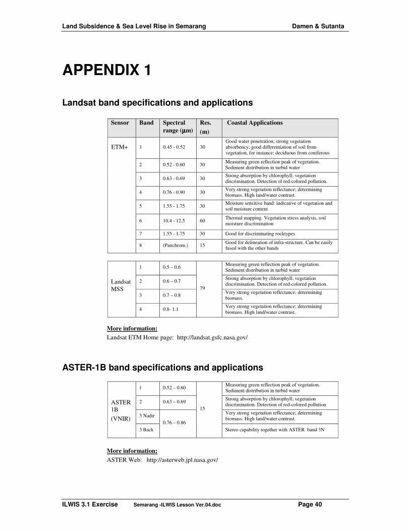
Land Subsidence & Sea Level Rise in Semarang Damen & Sutanta
ILWIS 3.1 Exercise Semarang -ILWIS Lesson Ver.04.doc Page 40
APPENDIX 1
Landsat band specifications and applications
Sensor Band Spectral range (µµµµm)
Res. (m)
Coastal Applications
ETM+ 1 0.45 - 0.52 30 Good water penetration; strong vegetation absorbency; good differentiation of soil from vegetation, for instance: deciduous from coniferous
2 0.52 - 0.60 30 Measuring green reflection peak of vegetation. Sediment distribution in turbid water
3 0.63 - 0.69 30 Strong absorption by chlorophyll; vegetation discrimination. Detection of red-colored pollution.
4 0.76 - 0.90 30 Very strong vegetation reflectance; determining biomass. High land/water contrast.
5 1.55 - 1.75 30 Moisture sensitive band: indicative of vegetation and soil moisture content
6 10.4 - 12.5 60 Thermal mapping. Vegetation stress analysis, soil
moisture discrimination
7 1.55 - 1.75 30 Good for discriminating rocktypes
8 (Panchrom.) 15 Good for delineation of infra-structure. Can be easily fused with the other bands
1 0.5 – 0.6 Measuring green reflection peak of vegetation. Sediment distribution in turbid water
2 0.6 – 0.7 Strong absorption by chlorophyll; vegetation discrimination. Detection of red-colored pollution.
3 0.7 – 0.8 Very strong vegetation reflectance; determining biomass.
Landsat MSS
4 0.8- 1.1
79
Very strong vegetation reflectance; determining biomass. High land/water contrast.
More information: Landsat ETM Home page: http://landsat.gsfc.nasa.gov/
ASTER-1B band specifications and applications
1 0.52 – 0.60 Measuring green reflection peak of vegetation. Sediment distribution in turbid water
2 0.63 – 0.69 Strong absorption by chlorophyll; vegetation discrimination. Detection of red-colored pollution
3 Nadir Very strong vegetation reflectance; determining biomass. High land/water contrast.
ASTER1B (VNIR)
3 Back 0.76 – 0.86
15
Stereo capability together with ASTER band 3N
More information: ASTER Web: http://asterweb.jpl.nasa.gov/
Land Subsidence & Sea Level Rise in Semarang Damen & Sutanta
ILWIS 3.1 Exercise Semarang -ILWIS Lesson Ver.04.doc Page 41

Land Subsidence & Sea Level Rise in Semarang Damen & Sutanta
ILWIS 3.1 Exercise Semarang -ILWIS Lesson Ver.04.doc Page 42
APPENDIX 2
Preliminary Assessment of the Impact of Land Subsidence and Sea Level Rise in Semarang, Central Java, Indonesia
By: HERI SUTANTA*), T.W. HOBMA**), M.J. DAMEN**), R.P.G.A. VOSKUIL**)
*) Department of Geodetic Engineering, Gadjah Mada University Jl. Grafika, no.2, Yogyakarta, Indonesia
Tel : 62-274-902121 Fax: 62-274-520226 e-mail: [email protected] **) Coastal Zone Studies, International Institute for Geo-information Science and Earth Observation (ITC),
Hengelosestraat 99, P.O. box 6, Tel : +31 (0)53 4874 285 Fax: +31 (0)53 4874 336 e-mail: [email protected]
ABSTRACT
Semarang city is suffering from two types of flooding, from rivers and high tides. The extend and magnitude of the floods seriously increased in recent years. This appears to be related to the ongoing processes of land subsidence and global sea level rise that this coastal city is faced with. The rate of subsidence in the city is varying, up to a maximum of 12 cm/yr. Medium estimates of sea level rise in the region indicate that the sea level in Indonesia will rise by 9, 13, and 45 cm for the years 2010, 2019, and 2070 respectively. To assess the combined effect of these phenomena and its spatial distribution, a procedure has been applied which combines up-to-date geo-information sources on terrain elevation and land use. A high accuracy Digital Terrain Model (DTM) has been generated using photogrammetrically-derived data. The present land use in the area has been assessed using high-resolution satellite imagery of Landsat-7 ETM+. The procedure has been developed and tested to calculate the impact of land subsidence and sea level rise on land use and population in a GIS environment. It aims to be applicable to other ‘sinking cities’ as well. The results for Semarang city indicate that the fishpond area (near the sea side) is the largest area to be affected, followed by the residential areas, bare land, agriculture fields and the industrial area. The economic and social consequences of the subsidence and the flooding are already felt and will be more severe in the coming decades. This study has served as a pilot for a research program in Semarang by ITC and partner institutes. This research focuses on methodology development in geo-information science for assessment, modeling and spatial planning of the urban coastal environment, under scenarios of sea level rise, land subsidence and flooding. Keywords: land subsidence, sea level rise, spatial modelling, geo-information science

ILWIS Exercise 1
INTRODUCTION Currently, coastal managers are facing a global challenge: How to manage the impact of global climate change? The most prominent impact of global change in the coastal zone is enhanced sea-level rise. Besides enhanced sea level rise, a related significant problem to many coastal cities is accelerated land subsidence. Coastal cities are often located in river deltas or in coastal plains. The subsurface of these unconsolidated deposits consists of sequences of clayey, peaty and sandy layers that have been deposited or developed under variable geological and hydrological conditions. Depending on land and water management practices, these coastal low lands presently show a complex spatial pattern in topography with areas subject to different rates of land subsidence (Hobma, 1999). Economic and population growth create a need for more space and resources. Land use in the coastal zone is changing very fast to meet the needs of large cities. In this process of transition the environmental capacity of the system and its sustainability is often neglected. The issue of the need for adequate fresh water supply to households and industry in the urban environment is high on the international agenda. This need is mostly fulfilled with pumping of groundwater. In many coastal cities over exploitation of groundwater is among the main causes of land subsidence. Semarang is the capital city of Central Java, Indonesia. It is situated on the North Coast of Java (Southern Latitude 6 o 56'08” to 7 o 06'57”, Eastern Longitude 110 o 16'17” to 110 o 30'31”; figure 1). The city covers an area of 373.73 sq. kilometers and acts as a center for regional government, industries, trade, education and tourism. The Directorate of Environmental Geology of Indonesia (2001) stated that there is evidence of land subsidence in Jakarta and Semarang, presumably due to the overexploitation of groundwater. The rate of subsidence in some parts of Semarang city is extremely high. Geodetic leveling measurements have been conducted in parts of the city. The results show that the northeastern part of the city has been subsiding by 20.5 cm in three years time (Basuki, 2000). The most obvious impact of land subsidence and sea level rise is flooding. There are two types of flooding in Semarang city: one is caused by river flooding (from the hinterland), the other is caused by the high tide (from the sea). Local people refer to the latter as rob.
108.00 108.50 109.00 109.50 110.00 110.50 111.00-7.50
-7.00
106.00 108.00 110.00 112.00 114.00
-8.00
-6.00
J A V A
Figure 1. Situation research area in Central Java.
River flooding occurs in the rainy season, from October to April. Rob occurs daily during high tide, and is sometimes enhanced by river flooding. It affects the transportation network as well as residential areas. A lot of houses have been abandoned already because people can not live there anymore. Some roads can only be used by big trucks. Despite their obvious impact, the issues of land subsidence and sea level rise have not been incorporated in city planning. Moreover, many inhabitants of Semarang do not know about the origin of the serious problems that their city is facing.
LAND SUBSIDENCE Land subsidence is the process by which the level of the ground is lowered from its previous elevation. It can be a result of natural phenomena as well as of man induced factors, or a combination of both. Factors that may cause land subsidence are e.g.: normal consolidation of clayey sediments; groundwater pumping; earthquake vibration; building loads; soil drainage and dewatering by canals. These impose either physical stress to the soil matrix or a fall in groundwater table, leading to desiccation of the soil. Under normal environmental conditions, a clay layer can be consolidated under its own weight. Groundwater pumping empties a clay layer’s pores so that it consolidates, which

Hazard study Semarang, Indonesia with ILWIS 3.1 Damen & Sutanta
File: Semarang -ILWIS Lesson Ver.04.doc 2
causes subsidence on the ground surface. The process is slow due to the limited permeability of the clay layer. According to the British Geological Survey (1998), the average piezometric head in Semarang has fallen by 20 m for a large part of the city, with a maximum of 27 m, since the early 90’s. This will result in a total consolidation of the clay layers by almost 5.5 m. The rate of consolidation follows a logarithmic trend. It is estimated that 50% of the total consolidation will occur in 12 years, and 90% in 50 years. The BGS research (1998) shows that the area with the largest fall in piezometric head is around the Terboyo industrial estate, on the east side of Semarang, where it exceeds the 20 m average fall up to a maximum of 25 m fall. In that situation, land subsidence could reach 5 m, which will cause severe damage to the area. The high fall in the piezometric level in that area is confirmed by the leveling measurements (Sutanta, 2002). These show that the area experiences a high subsidence rate, up to 12 cm/yr. The lowering of the groundwater level in Semarang is not only caused by extensive pumping but also by a decrease in groundwater recharge. In the upper part of Semarang, land use is changing rapidly from forest or rubber plantation to residential area (OME & DoEG, 1995). The Directorate of Environmental Geology (DoEG) and Office of Mine and Energy of Central Java (OME) have conducted subsidence monitoring for several years . They use the leveling technique of , which gives the highest accuracy among other subsidence measurement techniques. The measurements were carried out annually but, due to a limited budget, the entire area could not be measured in successive years. Each zone will, therefore, be re-measured with a couple of years time lag. This situation complicates the procedure of quickly making available information on the rate and the spatial distribution of the land subsidence. With scarce data, only 28 points could be selected from Tobing et. al (1999) and Basuki (2000), a map of the rate of subsidence has been created using interpolation by kriging (figure 2). The spatial pattern of the subsidence shows that the northern part of the city has higher rates compared to the southern part. The area is located near the industrial estate with extensive use of the groundwater.
Figure 2. Map of the rate of land subsidence. There are different rates of subsidence for different areas, for different years. This complexity arises from the dynamics of the natural phenomena and from human intervention, which in turn makes it difficult to find the most likely scenario of land subsidence in the entire area. A simplification has been made to determine the possible impact of land subsidence in the future. The rate of the land subsidence is assumed to be linear, and the latest data are used for the prediction, resulting in the map in figure 2.
SEA LEVEL RISE Global warming is thought to change the sea level through thermal expansion of the oceans and by changing the net mass balance of glaciers and ice sheets (Raper, et.al., 1996; Titus, 1990; Warrick, 1993). Global sea level data have been used to estimate the past sea level rise and to project future sea level rise. It was found, though, that there is variability in sea level data. This may be caused by e.g. (Gornitz, 1993 and Onselen, 2000):
• Data quality and distributions: tide gauges records are too short or variable in length, often with data gaps; abrupt changes in tide gauges locations; and lack of data from the southern hemisphere;
• Vertical land movement (tectonics and non-tectonics);

Introduction to ILWIS 3.1, using data from Semarang, Indonesia
ILWIS Exercise 3
• Measuring error of the tide gauge equipment; • Inaccuracies in the geodetic measurement used to connect the tide gauge to a local reference
frame; • Inaccuracies in the height connection between the local reference frame; • Coupled atmospheric and oceanographic effects, which include winds, waves, currents,
ocean temperature and salinity. Tidal data observations have been done in Indonesia since a long time for many purposes. This task is carried out, mostly, by government institutions e.g.: Bakosurtanal (Coordination Agency for Survey and Mapping); Ministry of Public Works; Hydro-Oceanographic Section of the Navy; and by Port Authorities. The analysis of sea level rise in Indonesia faces the problem of a lack of long and continuous records. The purposes of sea level measurements include: ship navigation, definition of local height datum, and long term monitoring for prediction of global sea level rise (Subarya, 2001). Table 1. Mean sea level data in Semarang from November 1998 to November 2000 (Bappeda, 2000).
Observation Nov-98 Dec-99 Nov-00 MSL (cm) 60.0 83.37 81.6
From the table we can draw the conclusion that the sea level is not in a static condition. The following variations have been observed between the years,
Nov 1998 to Dec 1999 : 23.37 cm Dec 1999 to Nov 2000 : - 1.74 cm
Sea level change in two years is,
Nov 1998 to Nov 2000 : 21.63 cm Those variations most likely resulted from other causes than global sea level rise. It is clear that the variation is very high, even exceeding the worst scenarios of global sea level rise (1 to 2 cm/yr). Possible causes for this include e.g.: instability of the tide gauge station and the benchmark to connect the station to the height system, and vertical land movement in the area. Titus & Narayanan (1995) propose a simple method to calculate local sea level rise. They propose to linearly extrapolate historical records and adding global projection to it. This will compensate for vertical land movement and inaccuracy in the projection of global sea level change. To avoid double counting, global projection should be corrected for the corresponding modelled trend of sea rise during the period of historical data. Local sea level rise by the year t for a particular location has been calculated using the following equation: local(t) = global(t) + (trend-0.12) . (t-1990) In this equation, trend is the current rate of relative sea level rise at the particular location. The value 1.2 mm/yr was based on the assumption of global sea level rise in the last century. The above formulae, however, could not be implemented for the situation in Semarang due to the fact that there is no information about the stability of the tide gauge station and the tide gauge benchmark. Therefore it has been decided to use a prediction from the study by the Asian Development Bank (1994) as a basis of the sea level rise scenarios. The influence of land subsidence will be treated separately. The projections for sea level rise from the year 1990 up to the year 2070 are listed in table 2. Table 2. Projection of changes in sea level in Indonesia as compared to 1990 (ADB, 1994)
Scenario 2010 2019 2070 Low 3 6 15 Medium 9 13 45 High 15 25 90

Hazard study Semarang, Indonesia with ILWIS 3.1 Damen & Sutanta
File: Semarang -ILWIS Lesson Ver.04.doc 4
LAND USE MAPPING The purpose of land use mapping from satellite data is to provide spatially distributed information on human activities and assets for the next processing stage. Extreme physical events, such as the present combination of flooding and land subsidence, may result in a disaster when there is an impact on a vulnerable society or human activity (Susman et al., 1983). Disasters can be quantified and predicted only insofar as the factors of the product ‘extreme event x vulnerable system’ are reasonably well known and quantified. In case of sea-level rise and population, only some terms of the equation are known: at the macro level, population growth is affected by the least error (Gommes et al., 1998). In this study a land use map has been derived from satellite image data and fed into a GIS for making such a risk assessment. The procedure involves spatial modelling with other map layers (DTM; population density) and dynamic parameters (rates of sea level rise and land subsidence). The remote sensing based land use mapping procedure has been applied because a sufficiently detailed map was not available. A Landsat-7 ETM+ image was taken on 2nd August, 2001 at 10 48’50” A.M., in 3 visible and 3 infra-red bands with 30 m resolution, and 1 panchromatic band with 15 m resolution. Ancillary data sets for the processing were: GPS points collected from the field and a topographic map made by Bakosurtanal. The topographic map was made on the basis of aerial photographs acquired in 1981 and a field survey in 1991. A Garmin Map handheld GPS was used to collect GPS point in the field. The accuracy obtained, as shown by the receiver, is between 3 to 6 m. This accuracy is still far below the pixel size of the image. Image fusion has been applied to sharpen the image and enhance certain features that were not visible in a single band image. Image fusion is an algorithm that combines two or more digital images to build a new image with modified digital numbers (Pohl, 1996). In this study, a statistical/numerical fusion method with linear combinations of Landsat band 5, 4, 2, and 8 has been applied. The fused image showed better results in the interpretation, in terms of spatial detail and observed transitions in the urban environment. Eight land cover types have been defined, which include: urban area, industrial area, fish pond, sea water, agriculture field, bare land, forest, plantation, and homestead garden. The supervised classification has been performed using the ILWIS v. 3.01 software package [ITC, 2002]. To remove isolated classes from the map, a majority filter has been applied. The filter selected the predominant class in a predefined window (3x3), and assigned that class to the unclassified or isolated pixel. Finally, the classification result has been assessed by creating a classification error matrix (or confusion matrix) and by calculating (‘Khat’) statistics. The overall accuracy for the land use classification of Semarang [Sutanta, 2002] is 84.95 %, with a Khat value of 0.899 (0-1).
DTM generation A Digital Terrain Model (DTM) is an ordered array of numbers that represents the spatial distribution of terrain characteristic (Doyle, 1978). This study makes use of photogrammetric DTM produced by Bakosurtanal, which is based on aerial photographs taken in 1994. The scale of the aerial photographs was 1:30000 and 1:50000. Breaklines and riverlines were included. Both DTM data were already checked prior to further processing (Amhar, 2001). However, the spots heights are not well distributed over the area. In the hilly and undulating areas the interval of the spot height is 100 m, while in the lowland and flat area the interval is 200 m. Some parts of the coastal area are under-sampled, without any or very limited number of spot heights. The under-sampled area may influence the final DTM, and, therefore, needed to be corrected. However, no measurements were available to fill the blank area. Inserting additional spot heights along the coastline has solved the problem. It was assumed that the coastline has a zero elevation. The area of major interest is the lowland part of the city. This area is entirely flat with low elevation. Therefore, the interpolation procedure aimed to give the highest possible accuracy for this area. The ‘Inverse Distance to a Power’ algorithm (available in Surfer v. 7.0) has been used in the interpolation process. A raster grid has been chosen as the data structure, because the resulting DTM had to be combined with the other data also having a raster (grid) structure. The grid size for the DTM was set to 15 m, according to the planimetric accuracy of the data and the highest spatial resolution of the satellite image. The quality of the DTM has been assessed by calculating root mean square (RMS) values of the elevation.
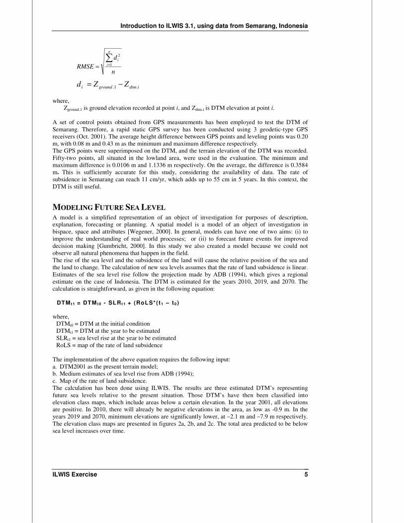
Introduction to ILWIS 3.1, using data from Semarang, Indonesia
ILWIS Exercise 5
where,
Zground.1 is ground elevation recorded at point i, and Zdtm.i is DTM elevation at point i. A set of control points obtained from GPS measurements has been employed to test the DTM of Semarang. Therefore, a rapid static GPS survey has been conducted using 3 geodetic-type GPS receivers (Oct. 2001). The average height difference between GPS points and leveling points was 0.20 m, with 0.08 m and 0.43 m as the minimum and maximum difference respectively. The GPS points were superimposed on the DTM, and the terrain elevation of the DTM was recorded. Fifty-two points, all situated in the lowland area, were used in the evaluation. The minimum and maximum difference is 0.0106 m and 1.1336 m respectively. On the average, the difference is 0.3584 m. This is sufficiently accurate for this study, considering the availability of data. The rate of subsidence in Semarang can reach 11 cm/yr, which adds up to 55 cm in 5 years. In this context, the DTM is still useful.
MODELING FUTURE SEA LEVEL A model is a simplified representation of an object of investigation for purposes of description, explanation, forecasting or planning. A spatial model is a model of an object of investigation in bispace, space and attributes [Wegener, 2000]. In general, models can have one of two aims: (i) to improve the understanding of real world processes; or (ii) to forecast future events for improved decision making [Gumbricht, 2000]. In this study we also created a model because we could not observe all natural phenomena that happen in the field. The rise of the sea level and the subsidence of the land will cause the relative position of the sea and the land to change. The calculation of new sea levels assumes that the rate of land subsidence is linear. Estimates of the sea level rise follow the projection made by ADB (1994), which gives a regional estimate on the case of Indonesia. The DTM is estimated for the years 2010, 2019, and 2070. The calculation is straightforward, as given in the following equation: DTM t 1 = DTM t 0 - SLR t 1 + (RoLS*(t1 – t0 ) where,
DTMt0 = DTM at the initial condition DTMt1 = DTM at the year to be estimated SLRt1 = sea level rise at the year to be estimated RoLS = map of the rate of land subsidence
The implementation of the above equation requires the following input: a. DTM2001 as the present terrain model; b. Medium estimates of sea level rise from ADB (1994); c. Map of the rate of land subsidence. The calculation has been done using ILWIS. The results are three estimated DTM’s representing future sea levels relative to the present situation. Those DTM’s have then been classified into elevation class maps, which include areas below a certain elevation. In the year 2001, all elevations are positive. In 2010, there will already be negative elevations in the area, as low as -0.9 m. In the years 2019 and 2070, minimum elevations are significantly lower, at –2.1 m and –7.9 m respectively. The elevation class maps are presented in figures 2a, 2b, and 2c. The total area predicted to be below sea level increases over time.
n
dRMSE
n
ii�
== 1
2
idtmgroundi ZZd .1. −=

Hazard study Semarang, Indonesia with ILWIS 3.1 Damen & Sutanta
File: Semarang -ILWIS Lesson Ver.04.doc 6
Figure 2. Elevation class maps for the years: (a) 2010, (b) 2019 and (c) 2070.
IMPACT ON LAND USE AND POPULATION The next step is to calculate areas at a certain elevation class. This calculation is based on the assumption that no is action taken to protect the area from subsidence or flooding.
Table 3. Areas below a certain elevation for the years 2001, 2010, 2019, and 2070 (Sutanta, 2002).
Area in years (ha) Elevation
class 2001 2010 2019 2070 < 0.0 m --- 1,270 2,302 5,597 < 0.5 m 1,260 2,947 3,985 6,697 < 1.0 m 3,559 4,881 5,676 7,746 < 2.0 m 6,674 7,201 7,525 8,949 < 5.0 m 9,352 9,610 9,790 10,400
The next step is then to calculate the area of specific land use types that fall within a certain elevation class. The land use data result from the supervised image classification procedure. Table 4 presents the results of the overlay operation of the maps of land use (col.) and elevation classes (row) for the present situation.
(a)
(b)
(c)

Introduction to ILWIS 3.1, using data from Semarang, Indonesia
ILWIS Exercise 7
Table 4. Land use (ha) per elevation class (Sutanta, 2002).
Area (ha) per elevation class Land use type <0.5 m <1.0 m <2.0 m <5.0 m
Fishpond 1,029 2,366 3,245 3,415 Residential 110 658 1,746 3,052 Bare land 83 264 453 558 Agriculture 49 296 1,062 1,897 Industrial 5 59 212 293 Dry-land 1 20 111 342 Plantation - - 2 65 The fishpond area covers the largest area at the lowest elevation (1,029 ha). This situation means that the fishpond area is very vulnerable to the impact of land subsidence and sea level rise. The likely impact will be further inundation of the fishpond area, making it useless and causing great economic loss and social disruption. The residential area is also prone to these hazards. At present, a total of 110 ha of residential area is situated in zones where the elevation is only 0.5 m above mean sea level (Tab. 4). The number of people to be directly affected by relative sea level rise and land subsidence is based on the size of the urban area that will be affected. The calculation of how many people live in a certain elevation class uses the following steps:
1. Calculation of the population density of each urban village. 2. Calculation of the urban area in each village; this was done by spatially overlaying the maps
of administrative boundaries and land use. 3. Calculation of the population density on each raster grid of each village. 4. Calculation of the population in each elevation class per urban village.
The results are presented in table 5. Table 5. People presently living in a certain elevation class (Sutanta, 2002).
Elevation class Number of people 0.0 - 0.5 m 8,300 0.5 – 1.0 m 63.000 1.0 - 2.0 m 95.000 2.0 - 5.0 m 128.000
> 5.0 m 1.007.000 Although most of the inhabitants of Semarang live in areas situated above 5 m from MSL, the numbers of people living in lower areas are also significant. There are more than 71,000 people living in areas situated below 1.0 m from MSL. These people are very vulnerable to many types of coastal hazards. Most of them live in the Northeastern part of the city, in areas that are subject to maximum land subsidence and sea level rise. It is observed that the urban growth in Semarang is in a horizontal direction. The use of high-rise buildings (apartments) is still not common. At present, there are no such buildings in the city. Considering the present concentration of the residential areas, it is likely that the total residential area that will be affected by land subsidence and sea level rise will increase in the future. With a growing population and a growing size of the urban area, the impact is predicted to be more severe.
CONCLUSIONS AND RECOMMENDATIONS This paper has shown the usefulness of geo-information technology (remote sensing and geographic information systems) to rapidly assess the combined impact of land subsidence and flooding by sea level rise on an urban population. The assessment is considered to be of a preliminary nature. It quantifies the extent of the vulnerable area and the number of people likely to be affected by these coastal hazards. The procedure is especially useful in areas with scarce data, as is the case in many (mega) cities in coastal zones in the developing world.

Hazard study Semarang, Indonesia with ILWIS 3.1 Damen & Sutanta
File: Semarang -ILWIS Lesson Ver.04.doc 8
The present assessment and vulnerability study illustrates that different aspects of scale, both in time and space, play an important role. Short-term, mostly local, interests should be taken into account, but also long-term, global developments. This requires a multidisciplinary approach in which spatial natural-scientific data form the basis for an integrated socio-economic and administrative elaboration. Having this in mind, the study has served as a pilot for a larger research program in Semarang that is currently being prepared by ITC and partner institutes in Indonesia. It has already led to a second pilot study that deals with the hydrological aspects of tidal flooding and river flooding in Semarang City. The focus of this ITC research program in ‘Multifunctional Use of Space’ (from 2003; Hobma, 2001) will be on methodology development in geo-information science for assessment, modeling and spatial planning of the urban coastal environment, under scenarios of sea level rise, land subsidence and flooding. It is advised to organize the future research work in a logical sequence of work packages (WP). These range from the assessment stage, through vulnerability studies and spatial modeling to the design of a strategy or a practical tool to improve spatial planning. Six WP’s have been defined that deal with aspects of: 1. Integrated assessment of socio-economic incentives and biophysical constraints on the multi-
functional use of space and needs for planning. 2. Geological and geotechnical assessment of the spatial distribution and the rate of coastal land
subsidence using 3d-GIS; 3. High quality DTM generation from earth observation data and monitoring dynamic change in a
coastal urban environment; 4. Multisensor satellite approach for assessment of river and tidal flooding in a coastal urban
environment, under enhanced sea level rise; 5. Spatially distributed hydrological modelling of river and tidal flooding in a coastal urban
environment, under enhanced sea level rise; 6. Design and evaluation of a Spatial Planning Support System for local urban planning, under
scenarios of land subsidence and flooding, using spatial multi-criteria analysis. The proposed WP’s and their interrelationships in a common methodology strive to support effective coastal zone management with high quality geo-information products and tools (Hobma, 1999).
ACKNOWLEDGEMENT The authors would like to acknowledge the following organizations: Indonesian Aeronautics and Space Institute (LAPAN), BAKOSURTANAL, BAPPEDA Semarang, Office of Mine and Energy Semarang, International Institute for Geo-information Science and Earth Observation (ITC), the Netherlands, and the Department of Geodetic Engineering, Gadjah Mada University, Yogyakarta. References ADB, 1994, Climate change in Asia: Indonesia Country Report On Socioeconomic Impacts of Climate Change
and a National Response Strategy, available from http://www.ccasia.teri.res.in/country/indo/impacts/tables.htm#tab2, accessed 22 May 2001.
Amhar, Fahmi., 2001, personal communication, staff at Bakosurtanal. BAPPEDA, 2000, Profile of Marine and Coastal Zone of Semarang (in Indonesian), BAPPEDA, Semarang. Basuki, S., 2000, Rate and trend of land subsidence in the eastern part of Semarang (in Indonesian), Media
Teknik, No. 3, 2000. British Geological Survey, 1998, Groundwater Quality Monitoring and Aquifer Control in Indonesia: seminar
and workshop, Bapedal, Semarang. Directorate of Environmental Geology, 1999, Land subsidence, available from
http://www.dgtl.dpe.go.id/hydro/subsidence.html, accessed 22 May 2001. Government of Indonesia, 1999, National Strategy-Action Plan of Climate Change, Final Report, Jakarta. Gornitz, V., 1993, Mean Sea Level Changes in Recent Years, in Warrick et.al., Climate and Sea Level Change:
Observations, Projections and Implications, Cambridge University Press. Gui-Shan Yang, T.W. Hobma, M. Damen and J. van Genderen, 2001, Assessment of coastal vulnerability to sea
level rise applying RS and GIS in the Yangtze River Delta, China. Coastal Management (accepted). Hobma, T.W., 1999, Ecohydrological basis for coastal zone management. PhD-Thesis Faculty of Earth Sciences,
Vrije Universiteit, Amsterdam. ISBN 90-75739-03-6, 230 pp. With appendices. Hobma, T.W., 2001, Integrated Coastal Zone Management as a vehicle to make ‘Multifunctional Use of Space’.
Discussion paper ITC, Renesse meeting, May 9-10, 2001. ITC, 2002. http://www.itc.nl/ilwis/default.asp ILWIS 3.0 User's Guide, ITC, Enschede, The Netherlands. Lillesand, T.M., Kiefer, R.W., 2000, Remote Sensing and Image Interpretation, John Wiley and Sons, New York.

Introduction to ILWIS 3.1, using data from Semarang, Indonesia
ILWIS Exercise 9
Office of Mine and Energy and Directorate of Environmental Geology, 1995, Final Report of Project on Monitoring of Groundwater Recharge of Semarang and its Surrounding (in Indonesian), OME and DoEG, Semarang.
Onselen, K.I., 2000, The influence of Data Quality on the Detectability of Sea-Level Height Variation, Publication on Geodesy, Netherlands Geodetic Commission, Delft.
Pohl, C., 1996, Geometric Aspects of Multisensor Image Fusion for Topographic map Updating in the Humid Tropics, ITC Publication Number 39, Enschede.
Raper, S.C.P., Wigley, T.M.L., Warrick, R.A., 1996, Global Sea Level Rise: Past and Future, in Sea-Level Rise and Coastal Subsidence: Causes, Consequences, and Strategies, Milliman, J.D., and Haq, B.U., (eds.), Kluwer Academic Publisher, Dordrecht.
Subarya, C., The Present Status of Indonesian Tide Gauge Network and Indonesian Permanent GPS Station Network, National Report to PSMSL, available from: http://www.pol.ac.uk/psmsl/reports.national+regional/indonesia.html
Sutanta, H., 2002, Spatial Modeling of the Impact of Land Subsidence and Sea Level Rise in A Coastal Urban Setting, case study: Semarang, Central Java, Indonesia, M.Sc. thesis (unpublished) at the International Institute for Geo-information Science and Earth Observation (ITC), the Netherlands
Titus, J.G., Narayanan, V.K., 1995, The Probability of Sea Level Rise, Environmental Protection Agency, Washington DC.
Tobing, MHL., EA. Syarief, D. Murdohardono, 1999, Research on Geo-technical Aspect of Land Subsidence in Semarang and its Surrounding (in Indonesian), Directorate of Environmental Geology, Department of Mine and Energy, Bandung.
Warrick, R.A., 1993, Climate and Sea Level Change: a Synthesis, in Warrick et.al., Climate and Sea Level Change: Observations, Projections and Implications, Cambridge University Press.