_________________

QuadTech, Inc.

Presented at TAGA 2014 conference

Assessment of the Sources for Disagreement

between Two Spectrophotometers

John Seymour

Keywords: inter-instrument agreement, spectrophotometer, calibration

Abstract

Agreement between different models of spectrophotometers is increasingly

being recognized as an issue in the industry. Brand owners are requesting color

tolerances that are in some cases too tight to be met when using different make

and model spectrophotometers along the supply chain. This often means that

printers are being required to purchase a different model of spectrophotometer

for each print buyer that they supply. It is a particular problem when printers

seek to improve accuracy (and efficiency) by incorporating spectrophotometers

into the press. Such inline spectrophotometers are necessarily of a different

design than hand-held devices.

This paper is part of ongoing work. The ultimate goal of this work is to develop

a way to reliably standardize one instrument to another. The assumption is that

understanding the physical nature of the differences between instruments will

lead the way to a standardization process that provides the best performance

without being prone to large errors.

In this paper, I look first at how well five spectrophotometers of different make

and model agree on what “black” is, and then on how well they agree on what

“white” is. Several differences have been determined, including rejection of

specular light, calibration of absolute white, aperture size, and goniophotometry.

With the exception of calibration of white light, the traditional models for

standardizing one spectrophotometer to another do not account for these

differences.

Thus, it is necessary to proceed with caution when attempting to standardize one

instrument to another. Standardization may actually worsen the agreement

between two instruments. At the very least, it is necessary to make sure that the

physical properties of the standardization set (the set of samples used to correct

one instrument’s readings to match another) are similar to the physical

properties of the samples to be measured. In particular, translucency and gloss

are important.

Previous Work toward Improving Agreement

There is no dearth of papers that describe techniques whereby measurements of

a set of samples can be used to characterize and correct for the disagreement

between two instruments. I will use the word “standardize” to refer to this

process. See, for example, Robertson (1986), Berns et al. (1997), Rich (2004),

Van Aken et al. (2000, and 2006), Chung et al. (2004), and Nussbaum et al.

(2011).

There is also no dearth of commercially available software for performing this

standardization. Software is available from X-Rite (two versions), DataColor,

CyberChrome, Color Science Consultancy, HunterLab, and ColorMetrix. See

Bibliography section for links to these companies.

On the other hand, there were three studies that gave cautionary advice. Butts et

al. (2006) tested two commercially available programs and came to the

following conclusion:

Both profiling programs [Maestro and NetProfiler] were able to

improve the inter-instrument agreement on BCRA tiles, but with

consistency only for their own instruments… Improvements in BCRA

agreement did not produce similar improvements in textile

agreement… A significant number of textile samples were adjusted in

the wrong direction and are in much worse agreement after profiling.

These results were not unexpected. Rich (2004) had this to say: “If the model is

built with only glossy tiles, such as the BCRA ceramic tiles, then matte

materials, like textiles, are poorly modeled.” Rich recommended a collection of

glossy semi-gloss, and matte, chromatic and achromatic (near neutral) samples

for the characterization.

Seymour (2013) came to similar conclusions when analyzing BCRA tiles to

determine the characterization:

[S]tandardization with a seemingly reasonable set of samples and a

seemingly reasonable underlying mathematical model can be a worthless

endeavor, and can often significantly worsen intra-model agreement… it

was found that the BCRA series II set of tiles is lacking in that it does not

provide for reliable differentiation between errors in nonlinearity and

wavelength shift… This suggests that the addition of a few well chosen

tiles to the BCRA set may improve their ability to standardize one

instrument to another.

What Can Go Wrong?

The list of potential reasons for two instruments to disagree is rather daunting

[Spooner, 1991].

Repeatability – There is an inherent variation from one measurement to another

even in the same instrument. This may be in the instrument itself, or it may be

because of positioning on a non-uniform sample.

Black level – Pure black should measure as 0% reflectance. Does it?

Rejection of scattered light – An instrument is potentially sensitive to ambient

light. It may differ from another in the degree that it rejects specular reflections

or light reflected from outside of the true sample area.

White level – Spectrophotometers need to have a white calibration to convert

their internal measurements into standard reflectance values. This calibration

relies on measuring a white calibration reference that has official reflectance

values.

Measurement geometry – The measurement of most samples depends on the

angle that the light hits it as well as the angle the light is measured. A small

difference in the angular distributions of illumination and detection may affect

measurements.

Nonlinearity – The detector and associated electronics have some inherent

nonlinearity. That is to say, twice the amount of light may not yield a

measurement twice as large. This is not likely the case with today’s technology,

but many of the other problems mentioned in this list may present themselves as

issues with nonlinearity.

Aperture size – There is a subtler problem when measuring objects that are

translucent. Incident light will spread laterally through the sample. The amount

of this light that is measured will depend on the size of the area that is

illuminated and the size of the area that is measured. There are actually two

physical areas, and the relationship between them can enhance or detract from

the ability of an instrument to agree with other instruments. For convenience

sake, I will set that discussion aside and lump all this into the category of

“aperture size”.

Wavelength alignment – A spectrophotometer is calibrated in the factory to

assign wavelengths to each spectral band of the instrument. Two instruments

could disagree on this assignment.

Bandwidth difference – Each channel of a spectrophotometer accepts a range of

wavelengths in each of its bins. The fact that there is a difference is obvious

when an instrument with a 10 nm spectral resolution is compared against an

instrument with a 20 nm resolution, but there are still potential differences

between two 10 nm instruments.

Fluorescence – If a sample fluoresces, the measurement of a color depends a

great deal on the spectral curve of the illumination. This issue has been

addressed with the introduction of the M1 condition in ISO 13655, but even so,

there is potential for disagreement due to implementation differences.

The mathematical models described in the literature recognize some subset of

these causes for disagreement, and seek to quantify them. The approach of all of

these methods is to lump all the measurements together, and let regression tease

out the discrepancies in instrument design or calibration that cause the

disagreement.

As shown in the paper by Seymour (2013), one difficulty with this approach is

that the instrumental discrepancies are often confounded. Misattribution of cause

can lead to an increase in any disagreements. This is particularly true when the

samples to be measured differ from the samples used to standardize.

General Outline of the Experiments

The approach in this experiment is to use samples chosen to isolate the

individual causes for discrepancies between spectrophotometers as much as

possible. These sets of samples were measured by all instruments in the test

group. Inter-comparison of the measurements was performed to determine the

sources of color measurement discrepancies.

Five spectrophotometers were used for this experiment. All spectrophotometers

were 0/45 or 45/0, handheld devices. They were selected based on two criteria.

First, they cover (presumably) a wide range of designs. Second, they were

convenient for me to borrow for this test! I regret that instruments from

additional manufacturers were not available.

Note that measurements were made in May of 2013, so some of the devices

were under manufacturer’s certification and others were not. This was

intentional. Despite all exhortations to routinely calibrate instruments, the fact

remains that a large number of instruments in the field are not up to date.

Manufacturer Model Serial # Date of

manufacture

Last

certification

X-Rite eXact 001120 Jan 2013 Jan 2013

X-Rite 939 02135 Oct 2010 Oct 2010

X-Rite 530 001390 ? Feb 2013

Gretag-

MacBeth Spectrolino 3.257-14124 June 2009 June 2009

X-Rite SpectroEye 3.264-27942 ? Jan 2013

Figure 1: The spectrophotometers used in these experiments.

Black level experiment

Theory

The purpose of the black level experiment is to assess the degree to which the

instruments agree on what “black” is. Five samples were selected which should,

in theory, all be very close to zero reflectance. Differences between the

instruments in the measurements point to specific differences between the

instruments.

Ugg light trap – I have constructed a light trap from a boot box. The cardboard

box is roughly 5” X 12” X 15”, with a light tight cover, painted flat black on the

inside and top. The top has a piece of wood about 1/8” thick glued to the

cardboard cover. This top has a 5 mm aperture which is chamfered from below.

If the illumination does not hit the edge of the hole, the light reflected back at

0/45 will be extremely small. Two instruments may differ in the measurement of

the Ugg light trap if either a) the Ugg aperture is not large enough, or b) the

instrument was not properly zeroed.

Ceram black glass reference – Lucideon (formerly Ceram, and previous to that,

BCRA) provided me with a black reference made of highly polished black glass.

Since the surface is glass, there is an obvious specular reflection on the order of

5%. For a spectrophotometer with illumination at 0°, this specular reflection

should be sent back directly to the illuminator, so the glass should be very dark

for a 0/45 instrument. The same reasoning applies to illumination at 45°.

The 45/0 measurements of this black glass are at the noise floor according to

Lucideon’s measurements, so any instrument should read very close to zero. If

an instrument does not read zero for the Lucideon target, but does read zero for

the Ugg light trap, then the instrument has inadequate specular light rejection,

which may be an issue with dirty optics or inadequate attention to scattered light

in the design. Light which reflects specularly from a flat surface should be

blocked from reaching the detector, but could still manage to make its way to the

detector.

Interstyle Ceramic black tile – I obtained a black tile from Interstyle Ceramics

which is of a different design than the black glass reference from Lucideon. This

tile is clear glass with a thickness of 5 mm, and with a rich black on the bottom.

If the tile is viewed with a focused light, the black back (as viewed through the

clear glass) is a dark gray with a matte appearance. The illuminated area will be

displaced by roughly 7 mm from the measurement plane when the light comes in

at 45°, so the measurements on this tile will depend on the illumination and

measurement aperture.

First surface mirror – A mirror would not generally be thought of as a black

object, but a first surface mirror should have zero reflectance when measured

with a 45/0 or 0/45 spectrophotometer. (A first surface mirror has its shiny part

on the top so that the reflection is not seen through the glass. If it is a truly good

mirror, then all the light coming in at 45° should reflect at 45° and be ignored by

the instrument. This is a more extreme version of the specular light rejection

test, since the mirror will reflect perhaps 90% of the incident light at the specular

angle.

X-Rite 939 light trap – The XRite 939 comes with its own light trap for

calibration. While this should in theory give identical results to the Ugg trap,

inter-comparison of the measurements of the two traps will provide a useful

cross-check of the effectiveness of the two light traps.

The first four samples were measured with all the instruments, and the fifth one

(the X-Rite light trap) measured where possible. Ten replicate measurements

were made with each sample and each instrument.

In theory, at least, all the instruments should agree, within the limits of

instrument repeatability, on the measurement of all the black samples.

Results

Summary of Results

The numbers in each cell of the table below represent the average reflectance

over all wavelengths and over ten replicated measurements.

Instrument 1 Instrument 2 Instrument 3 Instrument 4 Instrument 5

Ugg light

trap 0.007% 0.000% 0.008% 0.031% 0.165%

(0.089%)

X-Rite 939

light trap 0.010% 0.006% 0.024% 0.026% 0.065%

Ceram

black reference

0.011% 0.011% 0.024% 0.036% 0.104%

Interstyle black tile

0.016% 0.330% 0.248% 0.279% 0.541%

First

surface

mirror

0.045% 0.097% 0.100% 0.178% 0.645%

Table 2: Average reflectance of the samples as measured by all instruments

Note that I have intentionally not identified the instruments since the intent of

this paper is not to rate specific models, but rather to try to understand

differences between commonly found instruments. The order of the instruments

is not the same between Table 1 and Table 2.

I consider the first three black samples (the two light traps and the Ceram

reference) to be the most important. The other two (Interstyle tile and first

surface mirror) are diagnostic.

The numbers in the table are color coded based on magnitude. The decision of

how to color the numbers is based on asking a simple question: “If this much

reflectance were to be added to a patch with a density of 2.0D, then how much

would the density be lowered?” The numbers in the table are green if the amount

of drop is less than 0.01D. This is absolutely acceptable. The yellow numbers

would cause a drop of 0.01D to 0.02D. This is also acceptable, in my opinion.

The orange numbers represent a density drop to somewhere between 0.02D and

0.05D. I consider this borderline acceptable. The numbers in red represent a

density drop of more than 0.05D. I consider this unacceptable.

Results by Instrument

Instrument 1

The black measurements for the first instrument are good for all samples. The

first surface mirror has a somewhat larger number, suggesting that the

instrument does have a “small issue” with scattered light. On the other hand, the

first surface mirror test is moderately large. But, the first surface mirror has

roughly 15 times as much specular reflection as any ink, so I see no need to

correct this instrument for black level.

Instrument 2

The numbers on the three critical samples are all very good, so there clearly are

no issues with black level calibration. The first surface mirror number is a bit

high: 0.097% corresponds to a 2.00D patch being read as 1.96D. But, as stated

for Instrument 1, this is a pretty severe test.

The number for the Interstyle tile is quite large. The likely source of this

difference is that Instrument 2 has a larger aperture.

The Interstyle tile is clear glass with a black backing. The backing is a matte

black, so there is a small amount of light reflecting at all angles from the area

that is illuminated. My guess is that the first instrument has a fairly small

aperture compared with the thickness of the clear glass. The drawing in Figure 1

shows illumination that reaches the black backing quite far afield from the area

of detection. Even though the light reflected from the black backing heads out in

all directions, very little of it is accepted by the detector, since it is outside of the

cone of acceptance of the detector.

Figure 1: Instrument with a small measurement aperture cannot see the

illuminated area

Figure 2 shows my guess as to what the aperture of the second instrument looks

like on the tile. The illumination and detection angles are such that there is some

overlap of the area of illumination of the bottom of the tile and the area of

detection. Thus, a small amount of light is measured, despite the fact that the

black area reflects only perhaps a few percent of the incident light.

Figure 2: Instrument with a larger aperture sees part of the illuminated area

Note: The drawings show a 45/0 geometry. The same basic arguments apply for

0/45 just by swapping the light bulb and the detector. Also, the drawings show a

design with underfill, which is to say the area illuminated is smaller than the

area that is measured. This is a requirement in ISO 13655 to avoid problems

with light scattered in the substrate. Note that overfill is equivalent to underfill—

the illumination area could also be larger than the area of detection.

Additional Note: Failure of an instrument on this sample is not an indictment of

that instrument. The sample is outside of the realm of what a 45/0 instrument is

designed to measure. It is as if the instrument were held several millimeters

above the sample, rather than in contact.

Instrument 3

Instrument 3 is slightly worse than the first two instruments on the X-Rite black

trap and the Ceram black reference. While this is likely to be statistically

significant and is likely to have a physical cause, it is insignificant from a

practical standpoint.

From looking at the Interstyle tile and the first surface mirror, it would appear

that the aperture size and specular rejection are similar to the second instrument.

Instrument 4

The first three columns (measurements of the two light traps and the Ceram

black reference) show that there is a borderline issue with black level calibration

for the fourth instrument. These three numbers indicate that a 2.00D patch

would likely read between 1.985D and 1.989D. This is possibly worth correcting

for.

The measurement on the Interstyle tile says that the aperture is of a similar size

to the second and third instruments.

The measurement on the first surface mirror is a bit larger than specular

rejection of the second and third instruments, but again, this is a severe test. The

fact that the measurement on the Ceram black tile is virtually the same as that of

the two light traps shows that, for the worst case scenario of measuring ink, the

specular rejection of the fourth instrument is not an issue of any concern.

Instrument 5

I was perplexed that the readings for Instrument 5 on the two black traps were

different by a factor of three. This concerned me so the measurements on the

Ugg black trap were retaken. The second set of numbers is also in the table. The

range of black offsets correspond to a density loss on a 2.00D tile of anywhere

from 0.027D to 0.066D. My best guess is that the black level of this instrument

is drifting.

The Interstyle tile measurement of over 0.5% is indicative of the size of the

aperture. It has the largest aperture of the handheld instruments.

The first surface mirror reading of 0.645% is also a bit troublesome. If we take

the rule of thumb that a glossy ink will have about 1/15th the specular reflection

as a first surface mirror, then we would predict that the error due to incomplete

specular rejection would be on the order of 0.043%. This represents a drop in

density of nearly 0.02D for a 2.0D patch.

That in itself is perhaps not all that troublesome, but it makes me a bit concerned

that there could be additional issues with stray light that will necessarily be

difficult to correct for.

White level

Theory

“Pure white” is the next step up from black in terms of complexity. If the

spectrum of the white sample is relatively flat spectrally, then wavelength

calibration and spectral bandwidth should not affect the measurements. If the

white samples have nearly the same level of reflectance, then the linearity of one

instrument versus another should also not be a factor.

I chose eight white samples to assess the agreement between the

spectrophotometers.

Spectralon – Spectralon is highly reflective and spectrally flat. It is also very

matte.

Ceram white BCRA tile – The white BCRA tile is very white, but is also very

glossy.

Behr sheet chart – This is a set of six paint samples that are all white and

relatively close in color. They have six different levels of gloss. These samples

are not likely as bright as the Spectralon or BCRA white tiles, but they are not

likely to have a great deal of lateral diffusion. These were all measured with a

black backing.

Any disagreement between instruments on the measurements of these samples is

likely to be due to one of three causes: white calibration, instrument geometry,

or lateral diffusion. The set of paint samples should help diagnose a difference in

geometry.

Procedure

Each of the eight samples was measured with each of the five instruments. For

each of these forty combinations of sample and instrument, ten measurements

were taken in different locations within a ½” by ½” area. This should reduce any

variability due to sample non-uniformity or instrument repeatability.

Data scrubbing

I performed a test of the repeatability of the measurements. For each wavelength

(of measurements of one sample by one instrument), there are ten

measurements. I computed the standard deviation of these. This gave me a

collection of 30-some measures of repeatability. I averaged all these together to

get a single number indicative of the variability of that sample/instrument

combination.

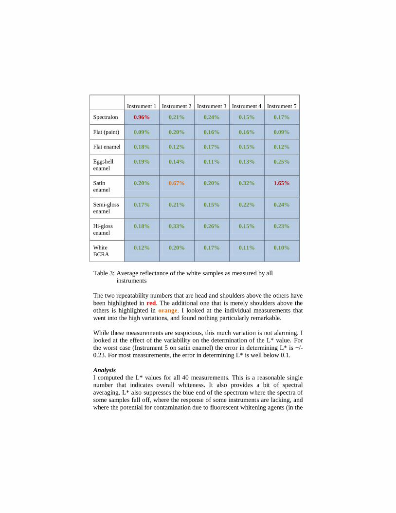
The results are shown in the table that follows. Note that, for example,

Instrument 3 measurements on the Spectralon sample had an average standard

deviation of 0.24%, meaning that a single measurement may vary by a few times

0.24% of, for example, 95.00% (i.e. the range could be from 94.52% to

95.48%). Note that the average of ten measurements will have repeatability of

one-third of this. Thus, the worst case uncertainty in the reflectance

measurements is ±0.55% (Instrument 5 on the satin enamel sample).

Instrument 1 Instrument 2 Instrument 3 Instrument 4 Instrument 5

Spectralon 0.96% 0.21% 0.24% 0.15% 0.17%

Flat (paint) 0.09% 0.20% 0.16% 0.16% 0.09%

Flat enamel 0.18% 0.12% 0.17% 0.15% 0.12%

Eggshell

enamel 0.19% 0.14% 0.11% 0.13% 0.25%

Satin

enamel 0.20% 0.67% 0.20% 0.32% 1.65%

Semi-gloss

enamel 0.17% 0.21% 0.15% 0.22% 0.24%

Hi-gloss

enamel 0.18% 0.33% 0.26% 0.15% 0.23%

White

BCRA 0.12% 0.20% 0.17% 0.11% 0.10%

Table 3: Average reflectance of the white samples as measured by all

instruments

The two repeatability numbers that are head and shoulders above the others have

been highlighted in red. The additional one that is merely shoulders above the

others is highlighted in orange. I looked at the individual measurements that

went into the high variations, and found nothing particularly remarkable.

While these measurements are suspicious, this much variation is not alarming. I

looked at the effect of the variability on the determination of the L* value. For

the worst case (Instrument 5 on satin enamel) the error in determining L* is +/-

0.23. For most measurements, the error in determining L* is well below 0.1.

Analysis

I computed the L* values for all 40 measurements. This is a reasonable single

number that indicates overall whiteness. It also provides a bit of spectral

averaging. L* also suppresses the blue end of the spectrum where the spectra of

some samples fall off, where the response of some instruments are lacking, and

where the potential for contamination due to fluorescent whitening agents (in the

substrate of the paint samples) exists. Finally, L* can be related to something

useful, ΔE. The assumption is that there is nothing interesting going on with a*

and b*.

The following graph shows all 40 measurements. The samples along the

horizontal axis are laid out in order of my perception of their gloss.

Figure 3: L* values of 8 samples as measured with 5 spectrophotometers

One of the measurements deemed anomalous because of variability

(Instrument 1 on Spectralon) shows up as anomalous in this chart as well. This

suggests that this point might be disregarded. The measurement with the largest

repeatability (Instrument 5 on satin) doesn’t appear to have an average value

which is all that anomalous.

This graph is a bit hard to comprehend. There is an overall downward slope

from left to right, which merely indicates that the glossier samples are a little

darker. This is likely for reasons unrelated to glossiness. The more important

thing to look at in this chart is that the various instruments have a spread of

around 1 ΔL* for each of the white samples.

The simplest of the possible explanations is that the white calibration is different

between the instruments. This could be the result of the “chain of traceability”.

Typically, a spectrophotometer manufacturer will have a white reference tile that

has been measured by a standards lab. These official measurements for this tile

are then used to calibrate the white point of a “golden instrument” at the

manufacturing facility.

Since there is an inevitable drift in the white level for any spectrophotometer,

manufacturers provide a white calibration tile that travels along with the

instrument. The reference values for this calibration tile are typically measured

with the golden instrument. Thus, there is an unbroken chain of traceability back

to a national standards lab, but each step in the chain adds uncertainty.

Another possible explanation is that the national standards labs do not agree

with each other as well as we might expect. There is very good agreement on the

size of a meter, a volt, and a second, but agreement on what constitutes 100%

reflectance is elusive. Thus, if one spectrophotometer manufacturer is traceable

back to the European standards lab, another to the Canadian, and a third to the

US lab, there is an inherent difference in white level.

So, perhaps the differences in the measurements of the white samples are due to

differences in white calibration?

Figure 4 addresses that question. The data was first “corrected” to calibrate to

the white BCRA tile. I arbitrarily decided that the correct Y value for the BCRA

tile was the average of the measurements from the six instruments. All the

measurements were then scaled so that the white BCRA tile had this arbitrary

measurement, and then converted to L* values. Next, I determined the deviation

from the average for each measurement. Thus, the y axis of the graph is a ΔL*

value.

Figure 4: L* deviations, after calibration to the BCRA tile

If we consider just Instruments 2, 3, and 5 on all white samples except for the

Spectralon, the agreement is under 0.5 ΔL*. Is this a problem? A change of 0.5

ΔL* on a white sample with L* = 97 corresponds to a scaling difference of

1.3%. That same scaling error will cause an error in L* that gradually gets

smaller as the measured sample turns from white to gray and then to black. The

ΔL* at L* of 75 is 0.42. At L* of 50, the error is 0.29. At L* of 10, the error is

0.12 ΔL*.

On the other hand, if we look at the extreme values, there is a 1 ΔL* difference

on all the paint samples. This is unfortunate, since BCRA tiles are often used to

calibrate instruments, and the range of gloss in the paint samples is similar to

that of ink on paper.

Why?

There are numerous possibilities for the large amount of disagreement. Many of

the possibilities can be put in the “not likely” pile simply by the selection of

samples. Each of the possible sources of disagreement is listed here, with an

explanation of whether this particular source is a candidate.

Instrument out of calibration – The spectrophotometers at the low end and at the

high end had been in for factory recertification within months of the data

collection, so this is not a likely problem.

Repeatability – In the previous section on data scrubbing, I reasoned that the

repeatability of my assessment of the average was “good enough”.

Black level – It is not likely that the differences are due to mis-calibration of

black level. The typical disagreement on a sample (after calibration to the BCRA

tile) from min to max was about 3% reflectance as compared with a maximum

light trap difference of 0.165%.

Rejection of scattered light – It is not likely that the differences are due to

rejection of specular reflection. The maximum number from an earlier

experiment was 0.645%. This number is still much less than 3%, it was only

found on one instrument (all the other instruments were considerably smaller),

and this number was on a first surface mirror, which has at least an order of

magnitude more specular reflectance than any of the samples.

White level – It seems likely that white level calibration is one source of

difference, but there are still significant differences with all instruments

calibrated to read identically on the white BCRA tile.

Measurement geometry – The samples were specifically chosen so as to vary in

gloss, so this is a likely candidate.

Nonlinearity – It is not likely that the differences are due to nonlinearity, since

all the measurements reported were between 88% and 96% reflectance.

Aperture size – There is likely some lateral diffusion in the samples tested, and

there is a difference in aperture size between the instruments, so this is a

possible source of disagreement.

Wavelength alignment or bandwidth difference – It is unlikely that the

differences are due to wavelength alignment or bandwidth, since the samples are

all reasonably flat over the Y region of the spectrum.

Fluorescence – It is not likely that the differences are due to fluorescence since

it is expected that there are no fluorescent whitening agents in any of the

samples. Using L* should mitigate any issues with fluorescence. Using the

eXact, I compared M0 and M2 measurements on all samples. The largest

difference over all the samples was 0.03 ΔL*.

In addition, I examined the effect of a violet laser (405 nm) on the samples. If a

sample has the typical fluorescence seen in paper, the laser will cause the

emission of light in the 420 to 450 nm range. This emission is very noticeable,

since the hue will shift from violet to blue, and the spot will appear much

brighter since the human eye is much more responsive at higher wavelengths.

While the paper underneath the paint samples was shown to fluoresce, there was

no evidence of any fluorescence in the samples themselves.

Based on this analysis, the three most likely candidates for disagreement are

1) white level calibration, 2) measurement geometry, and 3) aperture size. This

last possibility will be considered in the next section.

Aperture size

The question of whether differences in aperture size are responsible for

disagreement in measurement depends on two things. Obviously, the apertures

in the two instruments must be different. But also, the sample itself must be

susceptible to differences in aperture size, which is to say, the sample must have

an appreciable amount of lateral diffusion.

Images of the lateral diffusion

I used a red laser pointer and a digital camera to give a rough assessment of the

extent of the lateral diffusion in the white samples. I took pictures of a laser

pointer spot on three of the samples: the BCRA tile, one of the paint samples,

and the Spectralon tile. Only one of the paint samples was necessary, since they

all looked very similar. The magnification of the camera, the working distance,

and the f-stop were not changed in between samples.

I took an image of an aluminum plate to serve as a reference. My assumption is

that this plate shows an insignificant amount of lateral diffusion, so that the size

of the laser spot in the image is the actual size of the laser beam.

Figure 5: Laser spot on aluminum plate

The laser was hitting the sample at 45° and the camera was mounted at 0°. At

first glance, this may explain the ellipticity of the laser spot, but the aspect ratio

of the spot is close to 2.0, whereas, the 45° angle would put it at about 1.4. The

laser spot is fairly elliptical.

That said, I take the size of the laser beam to be about 3 mm wide.

Figure 6: Laser spot on BCRA tile

The BCRA tile (above) shows a laser spot that is not very different from the spot

on the aluminum plate. I will assume, then, that the BCRA tile has negligible

lateral diffusion, at least on the scale that I am able to measure.

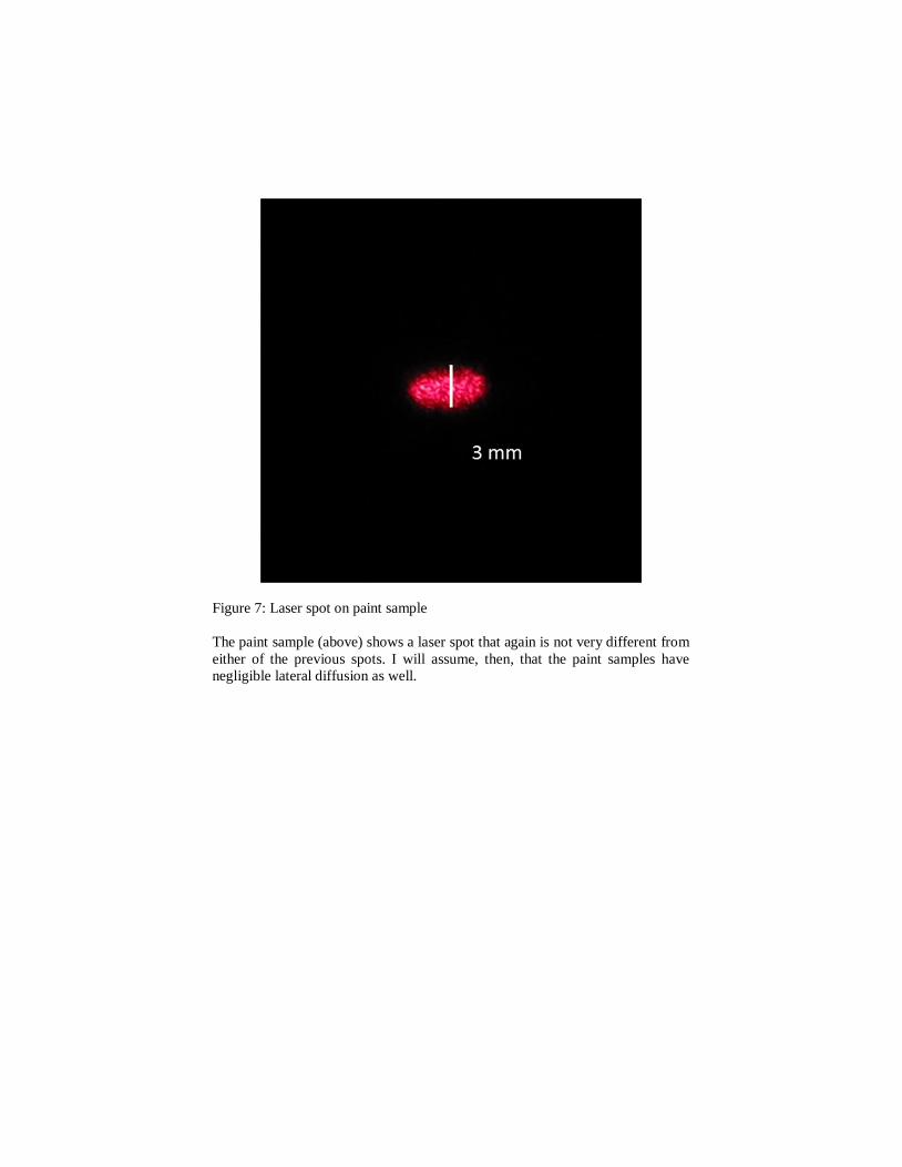
Figure 7: Laser spot on paint sample

The paint sample (above) shows a laser spot that again is not very different from

either of the previous spots. I will assume, then, that the paint samples have

negligible lateral diffusion as well.

Figure 8: Laser spot on Spectralon

The laser spot on the Spectralon sample is distinctly different, having a height of

about twice that of the other white samples. Based on this, it would seem that

Spectralon has a large degree of lateral diffusion.

There was a previous discussion about the measurement of Spectralon with

Instrument 1. The measurement looked anomalous. Was this real, or was it an

experimental error? The image of the laser pointer spot on Spectralon suggests

that this may be the explanation of the anomaly.

Looking back to the measurements on the Interstyle tile (Table 2, and Figure 1),

something unusual can be seen with regard to Instrument 1. This instrument

measured a very tiny reflectance on this tile (0.016%). This is a factor of 15

smaller than all the other instruments. This implies that the aperture of the

instrument is much different than the other instruments.

Thus, we can say that the anomalous measurement of the Spectralon sample

with Instrument 1 is real, and is a result of the combination of high lateral

diffusion of the sample and small aperture in the instrument.

Measurement geometry

The largest unexplained anomaly in Figure 2 is the response of Instrument 4.

This instrument reads darker than the rest of the pack. This discrepancy

gradually decreases with glossier samples. This particular instrument is not

greatly different from the others in terms of rejection of specular light (see

Table 2, first surface mirror reflectance). The dependence of the discrepancy on

gloss could be just the luck of the draw, or it could signal a goniophotometric

difference between this spectrophotometer and the others. That is, the

spectrophotometers differ in the angular distribution of the light hitting the

sample, or in the acceptance angle of the detector.

In the words of Sherlock Holmes, “Eliminate all other factors, and the one which

remains must be the truth.” Based on the fact that all other explanations that I

have to offer are unlikely, the mostly likely explanation of this difference is

goniophotometric.

Conclusion

Five spectrophotometers have been compared on measurements of black and

white samples which were selected so as to highlight the source of any

discrepancies. The findings are as follows:

1. PMZ calibration (setting of absolute black) is not a significant issue. A light

trap or a shiny black tile are both acceptable for calibration or for

verification of black level.

2. One instrument showed a larger issue with rejection of specular reflection,

this could be a small practical issue when measuring very dark samples.

3. The calibration of white level (overall scaling) is likely an issue. Standard

techniques for normalizing (standardizing, calibrating, profiling) one

instrument to another can correct this.

4. One instrument was different from the others in terms of its aperture.

Differences in the apertures of instruments are, in general, not correctable

through normalization of one instrument to another. On the other hand,

paint samples and presumably samples of ink on paper are not susceptible to

this discrepancy.

There are two areas for caution. First, measurement of translucent samples

(such as ink on milky plastics or white floodcoat, or inks with translucency)

will cause problems if the apertures differ between two instruments.

Second, one must use caution in selecting the samples that are used for

standardization. One common choice is the set of BCRA tiles.

Unfortunately, the yellow and orange tiles are known to have some amount

of lateral diffusion, so this is not advised.

5. One instrument shows evidence of differing from the others

goniophotometrically. Once again, these differences cannot be corrected for

in general, so caution must be employed when calibrating with samples that

differ in gloss from the samples one wishes to measure.

This paper has demonstrated that there are significant differences between

instruments that go beyond the standard calibration based on black level,

white level, nonlinearity, wavelength shift, and bandwidth differences.

There is a presumption that calibration can still be performed with these

techniques provided the calibration set has similar properties to the samples

to be measured, but this has not been investigated.

Bibliography

Berns, R.S., and Reniff, L.

1997, “An Abridged Technique to Diagnose Spectrophotometric Errors”,

Color Research and Application, 22(1), 51(10)

Butts, Ken, Brill, Mike, and Ingleson, Alan

2006 conference, “Reflectance in Perspective - Will Instrument Profiling

Give Me Better Measurements?”, American Association of Textile

Chemists and Colorists

http://industrial.datacolor.com/wp-content/uploads/datacolorproductliteratu

re/Reflectance%20in%20Perspective_40.pdf

Chung, Sidney Y., Sin, K.M., and Xin, John H.

2002, “Comprehensive comparison between different mathematical models

for inter-instrument agreement of reflectance spectrophotometers”, Proc.

SPIE 4421, p. 789

Nussbaum, Peter, Hardeber, Jon Y., and Albregtsen. Fritz

2011, “Regression based characterization of color measurement

instruments in printing application”, SPIE Color Imaging XVI

Rich, Danny

2004, “Graphic technology — Improving the inter-instrument agreement of

spectrocolorimeters”, CGATS white paper

Robertson, A. R.

1986, “Diagnostic Performance Evaluation of Spectrophotometers”,

presented at Advances in Standards and Methodology in

Spectrophotometry, Oxford, England

Seymour, John

2013, “Evaluation of Reference Materials for Standardization of

Spectrophotometers”, TAGA

http://johnthemathguy.com/files/pdf/Evaluation%20of%20Reference%20

Materials%20for%20Calibration%20of%20Spectrophotometers,%20Seym

our%20TAGA%202013.pdf

Spooner, David

1991, “Translucent Blurring Errors in Small Area Reflectance

Spectrophotometer & Density Measurement”, TAGA

Van Aken, Harold et al.

2000 U.S. Patent 6,043,894 (March 28, 2000)

2003 U.S. Patent 6,559,944 (May 6, 2003)

2006 U.S. Patent 7,116,336 (October 3, 2006)

Applications Mentioned:

CyberChrome OnColor profiler

http://www.cyberchromeusa.com/instrument-profiling/

ColorMetrix Normalizer

http://colormetrix.com/blog/normalizing-color-with-measure-parties-and-

outside-the-box-rd/

Color Science Consultancy Mean Plus

http://www.colorsciences.net/7209.html

DataColor Maestro

http://www.colourtechnology.eu/2008/upload/file/DataColor%20Meastro.pdf

HunterLab Hitch Standardization

http://hunterlabdotcom.files.wordpress.com/2012/07/an-1018-using-hitch-

standardization-on-a-series-of-color-measuring-instruments.pdf\

X-Rite NetProfiler

http://www.xrite.com/product_overview.aspx?ID=1765

X-Rite SpectroSync

http://www.xrite.com/documents/literature/en/L10-279_SpectroSync_en.pdf