Journal of Financial Economics 17 (1986) 223-219. North-Holland

ASSET PRICING AIVD THE BID-ASK SPREAD*

Received August 1985. tinal rsrsion received .~pril 1986

This paper studies the effect of the bid-ask spread on asset pricing. We analyze a model in which investors with different expected holding periods trade assets with different relative spreads. The resulting testable hypothesis is that market-obsewed expected return is an increasing and concave function of the spread. We test this hypothesis. and the empirical results are consistent with the predictions of the model.

1. Introduction

Liquidity. marketability or trading costs are among the primary attributes of many investment plans and financial instruments. In the securities industry, portfolio managers and investment consultants tailor portfolios to fit their clients’ investment horizons and liquidity objectives. But despite its evident importance in practice, the role of liquidity in capital markets is hardly reflected in academic research. This paper attempts to narrow this gap by examining the effects of illiquidity on asset pricing.

llliquidity can be measured by the cost of immediate execution. An investor willing to transact faces a tradeoff: He may either wait to transact at a favorable price or insist on immediate execution at the current bid or ask price. The quoted ask (offer) price includes a premium for immediate buying, and the bid price similarly reflects a concession required for immediate sale. Thus. a natural measure of illiquidity is the spread between the bid and ask

*We wish to thank Hans Stall and Robert W’haley for furnishing the spread data, and Manny Pai for excellent programming assistance. WC acknowledge helpful comments by the Editor. Clifford W. Smith. by an anonymous referee, by Harry DeAngelo. Linda DeAngelo, Michael C. Jensen. Krishna Ramaswamy and Jerry Zimmerman. and especiallv by John Long and G. William Schwert. Partial financial support by the lManageriaJ Economics Research Center-of the University of Roth .ster. the Salomon Brothers Center for the Study of Financial Markets. and the Israel Institute for Business Research is acknowledged.

0304~405X/86/53.50 S 1986. Elsevier Science Publishers B.V. (North-Holland)

prices, which is the sum of the buying premium and the selling concession.’ Indeed. the relative spread on stocks has been found to be negatively corre- lated with liquidity characteristics such as the trading volume, the number of shareholders. the number of market makers trading the stock and the stock price continuity.’

This paper suggests that expected asset returns are increasing in the (rela- tive) bid-ask spread. We first model the effects of the spread on asset returns. Our model predicts that higher-spread assets yield higher expected returns, and that there is a clientele effect whereby investors with longer holding periods select assets with higher spreads. The resulting testable hypothesis is that asset returns are an increasing and concave function of the spread. The

model also predicts that expected returns net of trading costs increase with the holding period, and consequently higher-spread assets yield higher net returns to their holders. Hence, an investor expecting a long holding period can gain by holding high-spread assets.

We test the predicted spread-return relation using data for the period 1961-1980, and find that our hypotheses are consistent with the evidence:

Average portfolio risk-adjusted returns increase with their bid-ask spread, and the slope of the return-spread relationship decreases with the spread. Finally, we verify that the spread effect persists when firm size is added as an explanatory variable in the regression equations. We emphasize that the spread effect is by no means an anomaly or an indication of market in- efficiency; rather, it represents a rational response by an efficient market to the existence of the spread.

This study highlights the importance of securities market microstructure in determining asset returns, and provides a link between this area and mainstream research on capital markets. Our results suggest that liquidity- increasing financial policies can reduce the firm’s opportunity cost of capital,

and provide measures for the value of improvements in the trading and exchange process.3 In the area of portfolio selection, our findings may guide investors in balancing expected trading costs against expected returns. In sum, we demonstrate the importance of market-microstructure factors as determi- nants of stock returns,

In the following section we present a model of the return-spread relation and form the hypotheses for our empirical tests. In section 3 we test the

‘Demsetz (1968) first related the spread to the cost of transacting. See also Amihud and Mendelson (1980.1982). Phillios and Smith (1982). Ho and Stoll(1981.1983). Coueland and Galai (1983). and‘west and Tinic (i971). For an ‘analysis of transaction costs in the context of a fixed investment horizon. see Chen. Kim and Kon (1975). Levy (1978). Milne and Smith (1980). and Treynor (1980).

‘See. e.g.. Garbade (1982) and St011 (1985)

‘See, e.g., Mendelson (1982.1985,1986.1987), Amihud and Mendelson (1985.1986) for the interaction between market characteristics, trading organization and liquidity.

predicted relationship, and in section 4 we relate our findings to the firm size anomaly. Our concluding remarks are offered in section 5.

2. A model of the return-spread relation

In this section we model the role of the bid-ask spread in determining asset returns. We consider M investor types numbered by i = 1.2.. . . , M, and N + 1 capital assets inds.;ed by i = 0, 1,2,. . . . N. Each asset i generates a perpetual cash flow of $d, per unit time (d, > 0) and has a relative spread of S,, reflecting its trading costs. Asset 0 is a zero-spread asset (S, = 0) having unlimited supply. Assets are perfectl? divisible. and one unit of each positive- spread asset i (i = 1.2.. . ., N) is available.

Trading is performed via competitive market makers who quote assets’ bid and ask prices and stand ready to trade at these prices. The market makers bridge the time gaps between the arrivals of buyers and sellers to the market, absorb transitory excess demand or supply in their inventory positions. and are compensated by the spread, which is competitively set. Thus. they quote for each asset i an ask price 7 and a bid price V,(l - S,). giving rise to two price vectors: an ask price vector (V,, V,, . . . . Vv) and a bid price vector (V,. V,(l - St) ,..., V,(l - S,v)).”

A type-i investor enters the market with wealth U: used to purchase capital assets (at the quoted ask prices). He holds these assets for a random, exponentially distributed time q with mean E[T] = l/p,. liquidates his port- folio by selling it to the market makers at the bid prices, and leaves the market. We number investor types by increasing expected holding periods,

PI -tQL~tl .** I/.$, and assets by increasing relative spreads, 0 = S, I S,I ... < S,v c 1. Finally, we assume that the arrivals of type-i investors to the market follow a Poisson process with rate X,, with the interarrival times and holding periods being stochastically independent.

In statistical equilibrium, the number of type-i investors with portfolio holdings in the market ha, a Poisson distribution with mean m, = X,/p, [cf. Ross (1970, ch. 2)]. The market makers’ inventories fluctuate over time to accommodate transitory excess demand or supply disturbances, but their expected inventory positions are zero, i.e., market makers are ‘seeking out the market price that equilibrates buyin 0 and selling pressures’ [Bagehot (?57i, p. 14); see also Garman (1976)]. This implies that the expected sum of investors’ holdings in each positive-spread asset is equal to its available supply of one unit.

Consider now the portfolio decision of a type-i investor facing a given set of bid and ask prices, whose objective is to maximize the expected discounted net

4Competition among market makers drives the spread to the level 3, of trading costs. In a different scenario. C; may be viewed as the sum of the market price and the buying transaction cost. and V, (1 - S, ) as the price net of the cost of a sell transaction.

cash flows received over his planning horizon. The discount rate p is the spread-free, risk-adjusted rate of return on the zero-spread asset. Let Y,, be the quantity of asset J’ acquired by the type-i investor. We call the vector

( .Y,,. i = 0.1.2.. . . . LV} ‘portfolio i’. The expected present value of holding portfolio i is the sum of the expected discounted value of the continuous cash stream received over its holding period and the expected discounted liquida- tion revenue. This sum is given by

=(p,+P)-‘ix~,[~,+P,Vi(‘-S,)l. J=o

Thus, for given vectors of bid and ask prices, a type-i investor solves the problem

max i x,,[d/+P,V,(l -s,)]. J-0

(1)

subject to

,v

c,y,,V,< W, and X,/LO forall j=O,1.2 ,..., N. J=o

(2)

where condition (2) expresses the wealth constraint and the exclusion of investors’ short positions.’ Under our specification, the usual market clearing conditions read

: m,x,,=l, j= 1,2...., iv (3) r-1

(recall that m, is the expected number of type-i investors in the market). When an A4 x (N + 1) matrix X* and an (N + l)-dimensional vector V*

solve the M optimization problems (l)-(2) such that (3) is satisfied. we call X * an equilibrium allocation matrix and V * - an equilibrium ask price vector

[the corresponding bid price vector is ( VO*, F’t*(l - S,), . . . , Vf(l - S,- )]. The

‘In our context. the use of short sales cannot eliminate the spread effect. since short >aIes b! themselves entail additional transaction costs. Note that a constraint on short po,itions ib necessary in models of tax clienteles [cf. Miller (1977). Litzenberger and Ramaswamy (1980)]. Clearly. market makers are allowed to have transitory long or short positions. but are constrained to have zero expected inventory positions [cf. Garman (1976)].

above model may be viewed as a special case of the linear exchange model [cf. Gale (1960)]. which is known to have an equilibrium allocation and a unique equilibrium price vector. Our model enables us to derive and interpret the resulting equilibrium in a straightforward and intuitive way as foilows.

We define the expected spread-adjusted return of asset j to investor-type i as the difference between the gross market return on asset j and its expected liquidation cost per unit time:

r ,,=d,/v,-Ir&

where d/V, is the gross return on security j, and p,S, is the spread-adjwt- ment, or expected liquidation cost (per unit time), equal to the product of the liquidation probability per unit time by the percentage spread. Note that the spread-adjusted return depends on both the asset j and the investor-type i (through the expected holding period).

For a given price vector V, investor i selects for his portfolio the assets j which provide him the highest spread-adjusted return, given by

r* = I

max r, ;, (5) j-0.1.2 . . . . . N 1

with r,* I r2” I r3* I . . . I r;, since, by (4), r,, is a non-decreasing function of i for all j. These inequalities state that the spread-adjusted return on a portfolio increases with the expected holding period. That is, investors with longer expected holding periods will earn higher returns net of transaction costs.6

The gross return required by investor i on asset j is given by r,* + p(S,. which reflects both the required spread-adjusted return r,* and the expected liquidation cost p,.S,. The equilibrium gross (market-observed) return on asset j is determined by its highest-valued use, which is in the portfolio i with the minimal required return, implying that

dj/V,* = mm r-1.2 .._.., v$* +PJJ.

Eq. (6) can also be written in the form

v,* = max r=l.Z . . . . . . M

{ d,/(r,* + p,s,)}9

(6)

‘This is consistent with the suggestions that while the illiquidity of investments such as real estate [Fogler (1984)] coins [Kane (1984)] and stamps [Taylor (1983)] excludes them from short-term investment portfolios, they are expected to provide superior performance when held over a long investment horizon (the same may‘apply to stock-exchange seats) [Schwert ( 1977)]. See also Day. Stall and Whaley (1985) on the clientele of small firms. and Elton and Gruber (1978) on tax clienteles.

implying that the equilibrium value of asset j. V, *. is equal to the present value of its perpetual cash flow, discounted at the gross return (rI* + p,S,). Alterna- tively, VJ* can be written as the difference between (i) the present value of the perpetual cash stream d, and (ii) the present value of the expected trading costs for all the present and future holders of asset j. where both are discounted at the spread-adjusted return of the holding investor. To see this, assume that the available quantity of asset j is held by type-i investors: then (7) can be written as

v/* = d/r,* - p,V,*S,/r,*,

where the first term is, obviously. (i). As .for the second, the expected quantity of asset j sold per unit time by type-i investors is p,. and each sale incurs a transaction cost of <*S,; thus, /.~,y*S,/r,* is the expected present value (discounted at r,*) of the transaction-cost cash flow.

The implications of the above equilibrium on the relation between returns,

spreads and holding periods are summarized by the following propositions.

Proposition I (clientele effect). Assets with higher spreads are allocated in equilibrium to portfolios with (the same or) longer expected holding periods.

Proof. Consider two assets, j and k, such that in equilibrium asset j is in portfolio i and asset k is in portfolio i + 1 (recall that I*, 2 p,_ r). Apply- ing (5), we obtain rI, 2 rrk and r,_ 1. k 2 r,_ I.,; thus, substituting from (4),

d,/V,*-I.r,S,2dk/V~-IL,Sk and dk/V~-~,,,SL)d,/~*-~,_lS,, im- plying that (IL, - p,*r)(Sk - S,) 2 0. It follows that if CL, > p,,r, we must have S, 2 S,. The case of non-consecutive portfolios immediately follows. Q.E.D.

Proposition 2 (spread-return relationship). In equilibrium, the obserced market (gross) return is an increasing and concave piecewise-linear function of the (relative) spread.

Proof. Let f,(S)= r,* + p,S. By (6) the market return on an asset with

relative spread S is given by f(S) = min,,,.z..,.. ,&(S). Now, the proposition follows from the fact that monotonicity and concavity are presemed by the

minimum operator, and that the minimum of a finite collection of linear functions is piecewise-linear. Q.E.D.

Proposition 2 is the main testable implication of our model. Intuitively, the positive association between return and spread reflects the compensation required by investors for their trading costs, and its concavity results from the clientele effect (Proposition 1). To see this, recall that transaction costs are amortized over the investor’s holding period. The longer this period, the

Market

Investor type, i return in excess

1 2 3 4 of p. the Value of asset Relative return 00 j relative to bid-ask

Length of holding period, p,-’

Asset, spread, l/12 l/2 1 5 the zero- that of the zero- spread spread asset.

i s, Excess spread-adjusted return. r,, - p asset v//v,

(1) (2) (3) (4) (5) (6) (7) (8)

0 0 101 0 0 0 0 1 1 0.005 1 0

L_l 0 0.05 0.055 0.059 0.06 0.943

2 0.01 3 0.015 - 0.05

l-l OS0 0.11 0.118 0.1’ 0.893 0.10 0.115 0.127 0.13 0.885

4 0.02 - 0.10 0.12

5 0.025 -0.155 W5 6 0.03 -0.21 0:09

0.12

7 0.035 - 0.265 0.085 8 0.04 - 0.324 0.076 D

0.136 0.11 0.877 0.140 0.145 0.873

0.12 0.144 0.15 0.870 0.12 0.148 0.155 0.866

,116 0.148 0.156 0.865 9 0.045 - 0.383 0.067 0.112 0 0.148 0.157 0.864

aIovestors have the same wealth, and the expected number of investors of each type is 1.

Y. A mhud and H. .Ylendelson. Asser prmng and the hrd-ash spread 22 9

Table 1

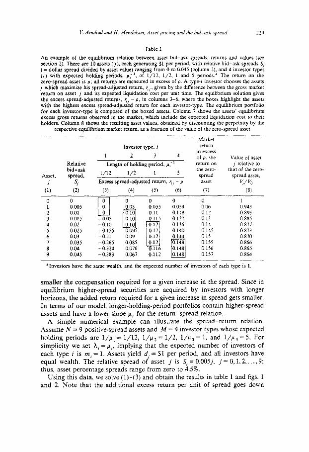
An example of the equilibrium relation between asset bid-ask spreads. returns and values (see section 2). There are 10 assets (j), each generating 51 per period, with relative bid-ask spreads S, ( = dollar spread divided by asset value) ranging from 0 to 0.045 (column 2). and 4 investor types (i) with expected holding periods, p;‘, of l/12. l/2, 1 and 5 periods.’ The return on the zero-spread asset is p; all re:urns are measured in excess of p. A type-i investor chooses the assets j which m aximixe his spread-adjusted return, r,,, given by the difference between the gross market return on asset j and its expected liquidation cost per unit time. The equilibrium solution gives the excess spread-adjusted returns, r,, - p, in columns 3-6, where the boxes highlight the assets with the highest excess spread-adjusted return for each investor-type. The equilibrium portfolio for each investor-type is composed of the boxed assets. Column 7 shows the assets’ equilibrium excess gross returns observed in the market. which include the expected liquidation cost to their holders. Co1um11 8 shows the resulting asset values, obtained by discounting the perpetuity by the

respective equilibrium market return, as a fraction of the value of the zero-spread asset.

smaller the compensation required for a given increase in the spread. Since in equilibrium higher-spread securities are acquired by investors with longer horizons, the added return required for a given increase in spread gets smaller. In terms of our model, !onger-holding-period portfolios contain higher-spread assets and have a lower slope ,LL, for the return-spread relation.

A simple numerical example can illus,;ate the spread-return relation. Assume N = 9 positive-spread assets and M = 4 investor types whose expected holding periods are 1,‘~~ = l/12, l/p2 = l/2, l/p”, = 1, and l/p4 = 5. For simplicity we set X, = p,, implying that the expected number of investors of each type i is m, = 1. Assets yield d, = Sl per period, and all investors have equal wealth. The relative spread of asset j is S, = O.OOSj. j = 0, 1,2,. . . ,9; thus, asset percentage spreads range from zero to 4.5%.

Using this data, we solve (l)-(3) and obtain the results in table 1 and figs. 1 and 2. Note that the additional excess return per unit of spread goes down

230 Y. A mlhud and H. .Men~elson .4sser pnwq und rhe hrd-usk spreud

investor

0 0.01 0.02 0.03 0.04 0.05 RELATIVE BID-ASK SPREAD

Fig. 1. An illustration of the relation between observed market return in excess of the return on the zero-spread asset (the excess gross return) and the relative bid-ask spread (see the numerical example of section 2 and table 1, column 7). There are 10 assets. each generating I$! per period. with relative bid-ask spreads (= dollar spread divided by asset va!ue) ranging from 0 to 0.045. and 4 investor types with expected holding periods ranging from l/l2 to 5 periods. Investors hav;

equal wealth. and the expected number of investors of each type is 1. The relation between asset returns and bid-ask spreads is piecewise-linear. increasing and

concave, with each linear section corresponding to the portfolio of a diRerent investor type.

from p1 = 12 in portfolio 1 to p2 == 2 for portfolio 2, then to pj = 1 in portfolio 3, and finally to p4 = 0.2 in portiolio 4. The behavior of the excess markt t return as a function of the spread is shown in fig. 1, which demonstrates both the positive compensation for higher spread and the clientele effect which moderates the excess returns, especially for the high-spread assets. This figure summarizes the main testable implications of our model: The observed market return should be an increasing and concave function of the relative spread. The piecewise-linear functional form suggested by our model provides a specific and detailed set of hypotheses tested in the next section. The effect of

the spread on asset values (or prices) is demonstrated in fig 2: the equilibrium values are decreasing and convex in the spread.

While the above model provides a lucid demonstration of th: spread-return (or spread-price) relation, our main results do not hinge on its specific form, and hold as well under different specifications. Consider (N + 1) assets, each generating the same stochastic (gross) cash flow given by the process ( X(t), r 2 O}. Assume that each transaction in asset j entails a cost of Scj, with 0 = cg < Cl < c* < * . . c cN (asset 0 having zero spread). There are M investor types numbered by i = 1,2,..., M, and the transaction epochs of type-i investors follow a renewal process with given parameters (depending on i).’

‘An investor could be viewed as owning a number of portfolios with different liquidation horizons, without changing the results.

Y. A mlhud and H. ,Mendelson. Asset pr~rng and rhe hrd-usk sprrud ‘?I

z Q 0.90 I 1:

Y * * * F

* * * * a 0.85

CK 0.80 I 1 I I I I I I I

0 0.01 0.02 0.03 0.04 0.05

RELATIVE BID-ASK SPREAD

Fig. 2. The relation between asset values and bid-ask spreads for the numerical example of section 2 (see table 1. column 8, and fig. 1). The figure depicts the value of each asset 1 relative to the value of the zero-spread asset, I$’ VO, as a function of the bid-ask spread relative to the asset’s

value. Asset values are a decreasing function of the spread.

Denote the highest price a type-i investor will pay for asset j by V,,. When the price of each asset j is determined by its highest-valued use, we have V,=max ,_1,2 ,_.,, ,Myj with 5, = V;, - c,8,, where 8, is the value (for investor- type i) of $1 at each transaction epoch. Letting f,(c) = &, - &I,, and follow- ing the arguments of Proposition 2, we obtain that the price [given by max r-1,2.....Mfr(C)l d is ecreasing and convex in c. Further. it can be shown that the price is a decreasing and convex function of the relative transaction cost, thus demonstrating the robustness of our results. Qualitatively, similar results will hold as long as a ionger investment horizon mitigates the burden of transaction costs by enabling their amortization over a longer holding period.

The next section presents empirical tests of our main testable hypotheses (Proposition 2).

3. Empirical tests

This section presents an empirical examination of the relation between expected returns and bid-ask spreads of NYSE stocks, focusing on the particular functional relationship predicted by our model. Specifically, our hypothesis is that expected return is an increasing and concave function of the spread.

732 Y. Amrhud and H. Mendelson. Asser prrcing and the bid-ask spreud

3.1. The data and the derivation of the variables

Our data consist of monthly securities returns provided by the Center for Research in Security Prices and relative bid-ask spreads collected for NYSE stocks from Fitch’s Stock Quotations on the IVYSE. The relative spread is the dollar spread divided by the average of the bid and ask prices at year end. The actual spread variable used, S, is the average of the beginning and end-of-year relative spreads for each of the years 1960-1979 [the data is the same as in Stoll and Whaley (1983)].

The relationship between stock returns, relative risk* (/3) and spread’ is tested over the period 1961-1980. Followin g the methodology developed by Black, Jensen and Scholes (1972), Fama and MacBeth (1973) and Black and Scholes (1974), we first formed portfolios by grouping stocks according to their spread and relative risk, and then tested our hypotheses by examining the cross-sectional relation between average excess return, spread and relative risk over time. We divided the data into twenty overlapping periods of eleven years each, consisting of a five-year fi estimation period E,, a five-year portfolio formation period F,, and a one-year cross-section test period T; (n = 1,2,..., 20).” The three subperiods of each eleven-year period are now consid- ered in detail:

(i) The beta estimation period E, was used to estimate the p coefficients from the market model regressions

R,‘, = a, + bj R’,, + El,, t=l ,...,60,

where R,‘I and RL, are the month-r excess returns (over the 90-day T-bill rates) on stock j and on the market,” respectively, and /3, is the estimate of the relative risk12 of stock j.

(ii) The portfolio formation period F, was used to form the test portfolios and estimate their ,8 and spread parameters. All stocks traded through the

‘By the CAPM, the p risk is the major determinant of asset returns. Our analysis in section 2 dealt with certainty-equivalent rates of return.

9The cost of transacting also includes brokerage commissions. In Stall and Whales (1983). the correlation between portfolio spreads and brokerage fees was 0.996, hence we omitted the la:ter.

loTo illustrate, EL = 1951-1955, Fl = 1956-1960, rt = 1961; E, = 1952-1956, F2 = 1957-1961, T2 = 1962; . . Ezo = 1970-1974, Fzo = 1975-1979, T,, = 1980.

“Throughout this study, R, and the test portfolios are equally weighted. See Black, Jensen and Scholes (1972). Fama and MacBeth (1973) and Stall and Whaley (1983, p. 71).

“Jensen (1968) has shown that the measure of relative risk, /3,, may be used for a holding period of any length (p. 189).

Y. Amhud and H. Mendeison. Asser pnang and rhe brd-ask spread 233

entire eleven-year period n and for which the spread was available for the last year of F, were ranked by that spread and divided into seven equal groups. Within each of the seven spread groups, stocks were ranked by their p coefficients, obtained from E,, and divided into seven equal subgroups. This yields 49 (7 x 7) equal-sized portfolios,t3 with significant variability of the spreads as well as the betas within the spread groups. Then, we estimated /3 for each portfolio from the market model regression over the months of F,,

R;, = ap + ,$,Re,r + ~~lr t=l ,..., 60, p=l,..., 49,

where R’pl is the average14 excess return of the securities included in portfolio p in month t. Finally, we calculated the portfolio spread S,, by averaging the spreads (of the last year of F,) across the stocks in portfolio p. Each portfolio p in period n is thus characterized by the pair (/I,,,, S,,) ( p = 1,2,. . . ,49, n = 1,2,. . . , 20). Altogether, we have 980 (= 49 x 20) portfolios.

(iii) The cross-section test period T, was used to test the relation between

$I’ Ppn and .‘$,_ across portfolios, where R;” is the average monthly excess return on the stocks in portfolio p in T,, the last year of period n.t’

Table 2 presents summary statistics for the 49 portfolio groups, classified by spread and 0. Note that both /3 and the excess return increase with the spread. The correlation coefficients between the portfolio excess returns RS, the portfolio betas & and the spreads SP, presented in table 3, show that both /?, and SP are posttlvely correlated with excess returns; the correlation between R; and the spread over the twenty-year period is about twice as high as that between R; and p. Also, note the high positive correlation between p and the spread.

3.2. Test methodology

We now turn to test the major hypothesis of model, namely, that expected return is an increasing and concave function of the relative spread. This is a classical case of covariance analvsis and pooling of cross-section and time-series data [see Kmenta (1971, ch. 12-2), Maddala (1977, ch. 14), Judge et al. (1980, ch. 8 )I, where the estimation model has to allow for differences over cross-sec-

13The long trading-period requirement might have eliminated from our sample the riskier and higher-spread stocks, thus reducing the variability of the data. Throughout, ‘equal’ portfolios may differ from one another by one security due to indivisibility.

“Throughout. averaaing means arithmetic averaging.

“Note that our tes; is predictive in nature. using estimates of risk and spread which are available at the beginning of the test period. See Fama (1976. 349-351).

Tabl

e 2

Ave

rag

e re

lati

ve

bid

-ask

sp

read

. m

on

lhly

ex

cess

ret

urn

. re

lati

ve

risk

(/

I) a

nd

li

rm

size

lo

r th

r 49

p

ort

folio

s fo

r Ih

e 20

lc

sr-p

erio

d

ycar

h

1961

-19

X0.

P

ort

folio

s ar

c in

dex

ed

by

the

spre

ad

gro

up

i

(I =

I f

or

the

smal

lesl

sp

read

) an

d by

~h

c b

eta

grou

p j

(j =

1 fo

r th

e sm

alle

st

beta

). Po

rtfo

lio

com

posi

tion

chan

ges

ever

y ye

ar

and

the

sam

ple

size

ran

ges

betw

een

619

and

YOO

sto

cks.

T

he

rela

tive

b

id-a

sk

spre

ad

of

a st

ock

is

iIs

do

llar

spre

ad

div

ided

b

y th

e av

erag

e o

f Ih

e b

id

and

as

k p

rice

s al

ye

ar

end

. T

he

po

rtfo

lio

aprc

ad

ib 1

11~

aver

age

rela

tive

sp

read

o

f st

ock

s in

Ih

e p

ort

folio

. T

he

po

rtfo

lio

(mo

nth

ly)

exce

ss r

etu

rn

is t

he

12-m

on

th

arit

hm

etic

av

erag

e o

f th

e m

on

thly

av

erag

e re

turn

s o

n t

he

sto

cks

in f

hc

po

rtt’

olio

in

cxc

~s

of

lhat

m

onth

’s

Trea

sury

-Bill

r~

hz.

The

port

folio

be

ta

is t

he

aver

age

rela

tive

risk

(/I)

co

ellic

ient

fo

r th

e st

ocks

in

th

e po

rtfo

lio.

c&m

ated

o

ver

rhc

5 ye

ar,

prc

ccd

ing

th

e ts

st

pcr

ictd

S

ize

is t

he

mar

ket

valu

e o

f th

e fi

rm’s

eq

uit

y in

mill

ions

of

dol

lars

al

lh

e en

d of

th

e ye

ar

prec

edin

g th

e W

I p

erio

d,

avcr

agcd

o

ver

the

tirm

r in

clud

ed

in

the

port

fool

io.

Spre

ad

grou

p,

I 2

3 4

5 6

7 M

ean

Beta

g

rou

p,

j

Sp

read

1 E

xces

s re

turn

B

eta

Siz

e

Sp

read

2 E

xces

s re

turn

U

ela

Siz

e

Sp

read

3 E

xces

s re

turn

B

eta

Siz

e

0.00

4765

0.

004X

SO

0.

004X

60

0.00

47x’

) o.

OO

4x7x

0.

0027

06

0.00

1306

0.

0033

80

0.00

44O

Y 0.

0034

27

0.54

001

0.67

797

0.75

890

0.77

867

0.X3

231

4089

.8

3245

.5

3231

.Y

2317

.3

1430

.0

___~

_~

~_ _

~ O

.W4X

Y I

O.W

5416

0.

9165

1 14

1x.x

0.1H

)4’J

XO

0.00

4X6

0.00

371(

1 No

C34’

J 1

WY7

3 0.

7’)‘)

5Y

5.7

2333

0.00

7435

0.

0074

45

0.00

7463

0.

0074

14

0.00

3174

0.

0035

43

0.00

354Y

0.

004Y

Y5

0.55

369

0.71

874

0.X1

652

llX45

Y6

780.

2 xx

o.3

74

1.5

707.

6

0.00

3050

0.

%)6

6X

656.

1

0.00

74

I2

0.00

7452

0.

0074

5 O

.(X)6

424

0.01

106

1 O

.(R)5

1 1

1.02

YYY

1.21

YY2

O.H

70

605.

Y 2X

2.7

665

0.00

9392

0.

0093

86

O.O

OY4

00

0.00

9375

0.

0093

19

O.O

OY3

50

0.00

9425

O

.oO

Y3Y

0.00

1838

0.

0031

65

0.00

6707

0.

0026

19

0.00

4473

0.

0061

33

0.00

5063

0.

0042

Y 0.

5606

9 0.

6727

1 0.

7954

3 0.

8986

6 1.

0035

7 1.

0451

x 1.

2094

0 o.

xx4

476.

2 50

2.1

695.

9 37

0.1

363.

Y 29

3.3

227.

1 41

x

Spread

4 Excess return

Beta

Size

Spread

5 Excess rclurn

Beta

Size

Spread

6 Excess return

Beta

Size

Spread

1 Excess return

Beta

Size

Spread

Mean

Excess return

Beta

Size

0.011470

0.011473

0.011411

0.011464

0.003217

0.002447

0.005296

0.004521

0.58821

0.69158

0.X4X2X

0.9220x

331.9

362.1

310.6

24X.4

0.014015

0.013913

0.0025X3

0.004340

0.60153

0.71lYl

243.1

251.3

0.013955

o.w331x

0.x2031

213.6

0.0139YX

0.013xx3

0.006763

0.00X076

O.Y2YO6

1.04923

166.3

14Y.2

0.017662

0.017513

0.0176')')

0.003637

0.006937

0.00720Y

0.65522

0.73861

0.87193

135.6

:31.1

127.1

0.017759

0.0177X9

0.007415

0.011254

0.94479

1.07714

113.1

91.2

0.032890

0.0293X5

0.006683

0.008876

0.76132

0.88340

15.2

67.8

0.031614

0.031472

0.031647

0.008044

0.007405

0.012335

0.99811

1.12656

1.2389Y

51.5

54.1

44.0

0.013947

0.013424

0.003405

0.004373

0.60867

0.72785

X76

778

0.013772

0.013753

0.0137Y2

0.005357

0.005447

0.007303

0.X4421

0.92083

1.01472

711

56X

426

0.01144Y

0.0114X7

O.OOXSO5

0.00X033

O.YY515

1.07535

250.5

192.4

0.013YbY

0.013YXX

0.011460

0.010266

1.12224

1.2XY27

146.2

111.3

0.017763

0.010x77

1.16769

X9.Y

0.033169

0.034385

0.0320X

0.013384

0.01492')

0.01024

1.33249

1.4625')

1.115

47.8

37.3

55

0.014006

0.014230

0.008X1X

0.009542

1.09X49

1.26161

399

214

0.011411

0.01145

0.00917x

O.OO5XY

1.2673'9

0.913

174.5

276

0.013Y6

O.oObbY

0.Y32

1x4

0.017'967

0.012516

1.334YX

72.X

0.01774

o.wx55

0.970

10')

0.013X5

0.00632

O.Y26

577

___

‘36 Y. A mthd und H. Mendelson. .Asset prmng und the hrd-usk spread

Table 3

Correlation coefficients between the annual average portfolio spread S,. excess return Rz and beta & for the entire sample period 1961-1980 and for its,two lo-year subperiods. 1961-1970 and 1971-1980. Portfolio spread is the average bid-ask spread as a fraction of the year-end average of the bid and ask prices for all securities in the portfolio. ELxcess returns are the a\-erage

monthly returns in excess of the monthly T-Bill rate.

Period

1961-80 1961-70 1971-80

Correlation coefficient between Number of R; and S, R’P and P, Pp and s, observations

0.239 0.123 0.361 980 0.179 0.132 0.163 490 0.285 0.118 0.540 490

tional units (portfolios) and over time. This is done by employing two sets of dummy variables: The first set consists of 48 portfolio dummy variables, defined by DP,, = 1 if the portfolio is in group (i, j) and zero otherwise; i= 1,2,..., 7 is the spread-group index and j = 1,2,. . . ,7 is the P-group index, with DP,,, = 0. By construction, the spread increases in i, and /3 increases in j. A second set of dummy variables, defined by DY, = 1 in year n (n = 1,2,..., 19) and zero otherwise, accounts for differences in returns between years.

An important implication of our model is that the slope of the return-spread relation declines as we move to higher-spread groups. To allow for different slope coefficients across spread groups, we decomposed the spread variable SP,, into seven variables Si,, (i = 1,2,. . . , 7) defined by Sp” = SP,, if in spread group i (i= 1,2,..., 7) and zero otherwise. Due to the high correlation between Si,,

and c:_, DP;,, we constructed the mean-adjusted spread variables, S;,, =

Sin - F if portfolio (p, n) is in group i and zero otherwise, where ?’ is the mean spread for the ith spread group. The means of S;,, are zero and their correlations with c’ ,_, DPij are zero. Replacing Sj” by the mean-adjusted variables thus leads to a separation between the level effects among groups (captured by DP,j) and the slope effects within spread groups (captured by

ii”). Using the above variables, we carried out the pooled cross-section and

time-series estimation of our model:

7 7 7 19

R;,, = a, + a& + c b;$, + 1 c c;,DP;, + c d,,DY, + ep,,, (8) 1-l i-l J’l n=l

where a,, aI, b,, c,, and d, are coefficients and the &pn are the residuals. The slope coefficients b, measure the response of stock returns to increasing the spread within spread group i, and the dummy coefficients c,, measure the

Y. Amrhud and H. Mendelson. .-lsxer pncmg and the hrd-ask spread 237

difference between the mean return on portfolio (i, j) and that of portfolio (7.7) which corresponds to the highest spread and ,!I group.

The sums cl_,c,, measure the differences in mean returns between ,f3

groups j, while X:_Ic,, measure the differences in mean returns between spread groups i. Thus, for any given /3, model (8) represents a piecewise-linear functional form of the return-spread relation. This follows the Malinvaud (1970, pp. 317-318) and Kmenta (1971, pp. 468-469) methodology for esti- mating non-linear relationships, which groups the data based on the values of the explanatory variable, and fits a piecewise linear curve using two sets of variables: group dummies to capture differences between group means, and products of the explanatory variable by the group dummies to allow for the different slopes.

Estimation of the pooled model (8) using OLS is problematic due to the possibility of cross-sectional heteroskedasticity and cross-sectional correlations among residuals across portfolio groups. While the estimated OLS coefficients are unbiased and consistent, their estimated variances are not, leading to biased test statistics. This calls for a generalized least squares (GLS) estima- tion procedure. Given that the variance-covariance matrix of the residuals in (8) is a’V, where u2 is a scalar and V is a symmetric positive-definite matrix, the GLS procedure uses a matrix Q satisfying Q’Q = V-’ to transform all the regression variables by pre-multiplication. The variance-covariance matrix V was assumed to be block diagonal (reflecting independence between years), where the diagonal blocks consist of twenty identical 49 X 49 positive definite matrices U. Then, V = I8 U, where I is the 20 x 20 identity matrix and 8 denotes the Kronecker product. To obtain the 49 x 49 matrix U, we first estimated model (8) by OLS and then used the data month by month to obtain the residuals 2,, (p = 1,2,. . . ,49) for each month m (m = 1.2.. . . ,240). Then, we estimated U by averaging the resulting 240 monthly variance-covariance matrices - the resulting estimate of the variance-covariance matrix V is known to be consistent [cf. Kmenta (1971, ch. 12)]. The transformation matrix Q was calculated using the Choleski decomposition method. The variables of model (8) were then pre-multiplied by the transformation matrix Q, and the transformed version of model (8) was estimated to provide the GLS results.

3.3. The results

We first ran a simple OLS regression of the excess returns on /3, the spread and the nineteen-year dummy variables:

REn = 0.0040 + 0.009478,, + E d, D Y, + epn,

(9.17j tY=-1

238

and

Y. .A mrhud and H. Mendelson. A ssel prrcrng and the hid-& yread

19

R’pn = 0.0036 + 0.0067213,, + 0.211S,, + 1 d, D Y,, + epn. (6.18) (6.83) ?I=1

(r-statistics are in parentheses.) The results show that excess returns are increasing in both p and the spread. The coefficient of S,,, implies that a 1% increase in the spread is associated with a 0.211% increase in the monthly risk-adjusted excess return. The coefficient of p declines when the spread variable is added to the equation, indicating that part of the effect which could be attributed to p may, in fact, be due to the spread.16 The coefficient of fl is 0.00672, very close to 0.00671, which is the average monthly excess return on common stocks for this period.

Next, we estimated the detailed model (8) using both OLS and GLS. The slope coefficients of the spread variables are presented in table 4, and the coefficients of DP,, are given in table 5. To estimate the pattern of the dummy coefficients, we employed the model

6 6

c ,,=a+ cv,DS,+ xS,DB,+e,,, 1=1 J=l

where the spread dummy DS, (i = 1,. . . , 6) is one if the portfolio is in spread group i and zero otherwise, and the /3 dummy DBj (j = 1,. _ _ ,6) is one if the portfolio is in fi group j and zero otherwise. Thus, the coefficients y, in (9) measure the difference between the average return of spread group i and that of the seventh (highest) spread group, and the coefficients 8, measure the corresponding differences between fl groups.

The estimates of (g)-(9) presented in tables 4 and 6 support our two hypotheses:

(i) The coefficients y1 of DS, in model (9) are negative and generally increasing in i, implying that risk-adjusted excess returns increase with the spread. The difference in the monthly mean excess return between the two extreme spread groups is 0.857% when estimated by OLS and 0.681% when estimated by GLS.

(ii) The slope coefficients of the spreads, b,, are positive and generally decreasing as we move to higher spread groups. This is consistent with the hypothesized concavity of the return-spread relation, reflecting the lower sensitivity of long-term portfolios to the spread.

‘6Given the strong positive correlation between Sp_ and &,,, the omission of Sp” from the regression equation which tests the CAPM results in an upward bias in the estimated coefficient of p; see Kmenta (1971. p. 392).

Estimatrd regressions of the portfolio monthly excess returns. R’. on the meanadJusted spread variables s” and relative risk. B. for the vears 1961-1980. usina ordinan least sauares and generalized least squares estimation methods. The regression m&e1 (8)’ apphes pooled cross-

section and time-series estimation. The coefficient of F reelects the response of stock returns to an increase in the bid-ask spread

within spread group I, where L = 1 corresponds to the louest-spread group. (r-values are in parentheses).

Table 4

Independent variable

Ordinary least squares coefficients

Entire period 1961-1980

Generalized least squares coefficients

Entire period Subperiod Subperiod 1961-1980 1961-1970 1971-1980

3.641 (2.76)

3.242 (3.50)

2.854 (3.93)

1.657

(3.06)

2.224 (5.69)

1.365 (5.28)

0.605 (5.28)

- 0.0058 (2.53)

1.310 (1.16)

1.747 (2.56)

1.660 (3.01)

0.482 (1.16)

1.206 (3.84)

0.650 (2.96)

0.256 (2.56)

-o.OOil (0.10)

0.080 (0.05)

0.975 (0.91)

0.934 (1.10)

- 0.149 (0.21)

0.922 (1.67)

0.838 (2.21)

0.176 (1.49)

- 0.002 (0.47)

2.303 (1.27)

2.505 (2.41)

2.27 (2.80)

0.983 (1.69)

1.500 (3.47)

0.475 (1.50)

0.489 (2.49)

- 0.003 (0.72)

“The regression model is

(8)

where Rf;, is the average excess return for portfolio p in year II. /3,, is the average portfolio relative risk. .?& is the mean-adjusted spread within spread group I ( = the deviation of the spread of portfolio p m year n from the mean spread of its spread group. I). DP,, are the portfolio-group dummy variables ( = 1 in portfolio group (i, j), zero otherwise). D Y, are the year dummy variables ( = 1 in year n, 0 otherwise), and rpn are the residuals. The GLS estimated coefficients of the portfolio-group dummies DP,, are reported in table 5.

The effect of the relative risk is measured in model (8) by both p and the dummy variables and is further summarized by the DB, coefficients of model (9). The emerging pattern is that (spread-adjusted) excess returns increase with /3 as depicted by the significant negative and increasing coefficients 6,. The effect of ,B is captured mainly through the dummies rather than the coefficient CI,, which is highly insignificant in the GLS estimation. Finally. we estimated

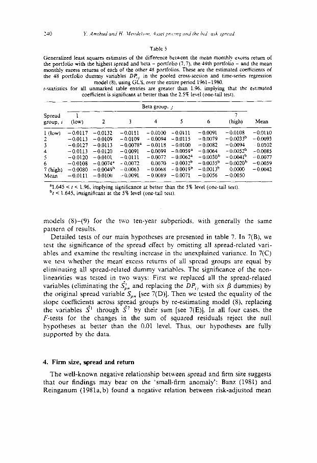
Table 5

Generalized least squares estimates of the difference between the mean monthly excess return of the portfolio with the highest spread and beta - portfolio (7.7), the 49th portfolio - and the mean monthly excess returns of each of the other 48 portfolios. These are the estimated coeRicients of the 48 portfolio dummy variables DP,, in the pooled cross-section and time-series regression

model (8). using GLS. over the entire period 1961-1980. r-statistics for all unmarked table entries are greater than 1.96, implying that the estimated

coefficient is significant at better than tb.e 2.5% level (one-tail test).

Spread 1 group, i (low) 2 3

Beta group. J

4 5 6 Mean

1 (low) -0.0117 -0.0132 -0.0111 -0.0100 -0.0111 - 0.0091 - 0.0108 2 -0.0113 -0.0109 -0.0109 -0.0094 -0.0115 -0.0079 -0.0033b 3 -0.0127 -0.0113 -0.0078’ -0.0118 -0.0100 -0.0082 -0.0094 4 -0.0113 -0.0120 - 0.0091 - 0.0099 - 0.0059= - 0.0064 - 0.0052b 5 - 0.0120 - 0.0101 -0.0111 - 0.0077 -0.0062a - 0.C030b - 0.0041b 6 -0.0108 -0.0074= -0.0072 -0.0070 -0.0032b -0.003Sb -0.0020b 7 (high) -0.0080 -0.tI1049~ -0.0063 -0.0068 -0.0019b -0.0013b 0.0000 LMean -0.0111 -0.0100 -0.0091 -0.0089 -0.0071 - 0.0056 - 0.0050

a1.645 c I < 1.96, implying significance at better than the 5% level (one-tail test). bf < 1.645. insignificant at the 5% level (one-tail test).

- 0.0110 - 0.0093 - 0.0102 - 0.0085 - 0.0077 - 0.0059 - 0.0042

models (g)-(9) for the tvvo ten-year subperiods, with generally the same pattern of results.

Detailed tests of our main hypotheses are presented in table 7. In 7(B), we test the significance of the spread effect by omitting all spread-related vari- ables and examine the resulting increase in the unexplained variance. In 7(C) we test whether the mean’ excess returns of all spread groups are equal by eliminating all spread-related dummy variables. The significance of the non-

linearities was tested in two ways: First we replaced all the sprea.d-related variables (eliminating the $,‘” and replacing the DP,, with six p dummies) by the original spread variable S,,, [see 7(D)]. Then we tested the equality of the slope coefficients across spread groups by re-estimating model (8), replacing the variables s^’ through s^’ by their sum [see 7(E)]. In all four cases, the F-tests for the changes in the sum of squared residuals reject the null hypotheses at better than the 0.01 level. Thus, our hypotheses are fully supported by the data.

4. Firm size, spread and return

The well-known negative relationship between spread and firm size suggests that our findings may bear on the ‘small-firm anomaly’: Banz (1981) and Reinganum (1981a, b) found a negative relation between risk-adjusted mean

Table 6

Regression estimates of the difference between the mean return of the spread and beta groups and the mean return of the highest-spread and highest-beta portfolio. The estimation model is

6 6

c,, =i a -r &,DS,+ CF,DB,-e,,. (9) r-l 1-L

where c,, are the dummy coefficients estimated from model (8) (table 5); DS, = 1 for the ~th spread group and zero otherwise; and DE, = 1 for the jth beta group and zero otherwise. Spreads

are increasing in i, and betas are increasing in 1. (r-statistics are in parentheses).

Estimated regression coefficients

Independent variable

Entire 1961-1980 period Subperiods

From OLS From GLS 1961-1970 1971-IYXO regression regression GLS GLS

DS,

DS,

DS,

DS,

DSj

DS,

DB,

DE2

DB,

DB,

DB,

DB,

- O.OOPj7 (9.05)

- 0.00654 (6.90)

- 0.007’9 (7.70) -

- 0.00552 (5.83)

- 0.00461 (4.86)

- 0.00’52 (2.66;

- 0.00964 (10.1X)

- 0.00767 (8.10)

-0.006’6 (6.61)

- 0.00568

(6.00)

- 0.00336 (3.55)

- 0.00147 (1.56)

-0.00681 (7.74)

- 0.00517 (5.X8)

- 0.00599 (6.82)

- 0.00439 (4.99)

- 0.00359 (4.08)

- 0.00172 (1.95)

- 0.00614 (6.9X)

- 0.00500 (5.68)

- 0.0041 I (4.67)

- 0.00398 (4.53)

- 0.00214 (2.43)

- 0.00065 (0.74)

- 0.00730 (7.46)

- 0.00578 (5.91)

- 0.00556 (5.69)

- 0.00446 (4 56)

- 0.00335 (3.43)

- 0.00246 (2.52)

- 0.00669 (6.84)

- 0.00495 (5.06)

- 0.00325 (3.31)

- 0.00260 (1.66)

- 0.00098

(1.00)

0.00017 (0.18)

- 0.00397 (3.33)

- 0.002h7 (2.21)

-0.004X3 (4.05)

- 0.00301 (2.53)

- 0.00273 (17.210

0.0005 1 (0.41,

- 0.00454 (3.81)

- 0.0042.1 (3.53)

- 0.00434 (3.64)

-0.004X5 (4.07)

- 0.002Y3 (3.46)

-0.00121 (1.01)

returns on stocks and their market value, indicating either a misspecitication of the CAPM or evidence of market inefficiency [see Schwert (1983) for a comprehensive review], Thus, it is instructive to estimate the effects of a firm-size variable and to test its significance vis-a-vis our variables.

We re-estimated our models adding a new explanatory variable - SIZE, the market value of the firm’s equity in millions of dollars at the end of the year

Table 7

Tests of hypotheses on the return-spread relation. All regressions are estimated bv GLS

Model”

Degrees of freedom of the model

SSR, sum of squared residuals

Difference from model (A)h

DF SSR .MS Fu

statistic

(4 75 76.7877 (B) 26 85.5459 (C) 33 83.3506 (D) 27 84.7339 (E) 69 78.4249

“The regression models are as follows.

Model (A) - the full model:

- 49 8.7612 0.17XR 2.10 42 6.5629 0.1563 1.x4 48 1.9462 0.1655 1.95

6 1.6372 0.2729 3.21

R;” = a0 + al& + &,i;,- i i c,,DP,,+ f d,DYn++Epn. i-1 r-l /‘I n=l

where p = 1.2,. ,49, n = 1.2. .20. and DP,, 3 0.

Model (B) - a restricted model for testing the existence of any spread effect:

(8)

6 19

RC,,=ao+alBp,+ c u,DB,+ Cd,DY,++.

J-1 n-l

Model (C) - a restricted model for testing the equality of mean excess returns across spread groups:

R>,=a,+a,&,,+ ib,.$,+ $y,DB,+ fd,DYn+Ep,. 1-l 1-1 “=I

Model (D) - a restricted model for testing the non-linearity of the return-spread relation: 6 19

R;” = a0 + al& + azsp, + C~,DB,+ c d,DY,+E Pn /=I !I=1

Model IE) - a restricted model testing the equality of the slope coefficients across spread groups:

R’pn = a0 f aI S,,, + a2

The regression variables are:

R:” = average portiolio excess return (the dependent variable) for portfolio p in year n.

B p” = average portfolio relative (8) risk,

San = average portfolio relative spread.

Sin = mean-adjusted spread (the deviation of the spread S,,” of portfolio p in year n from the mean spread of its spread group, i),

DP,, = portfolio group dummy; one in portfolio group ( r, j ). zero otherwise.

DY, = year dummy: one in year n, zero otherwise.

DB, = /3 group dummy; one in /3 group j, zero otherwise. DB, = c:_, DP,, (j = 1,2.. .6).

bData for the F-test on each of the restricted models:

DF = difference in the number of degrees of freedom between the full and restricted model. SSR = difference in the sum of squares between the full and restricted model, MS = SSR/DF. the mean square.

Y. Amrhud and H. .Mendelson. .-lsser prrcing und the brd-usk spread 243

just preceding the test period. As seen in table 2, there is a negative relation- ship between SIZE and both spread and /3. The effect of firm size on stock returns was tested by incorporating SIZE in all our models, but its estimated effect was negligible and hi&y insignincant.

To aIlow for a possible non-linear effect (as other studies do), we replaced SIZE by its natural logarithm and examined the impact of adding log(SZZE) to our regression equations. First, we estimated the simple linear model

R;,, = 0.0082 + 0.0060/3,, + O.lSSS,, + 0.0006 log( SIZE),, (5.05) (3.44) (1.56)

19

+ c d,DY,+ epn. n=l

The results indicate that the risk and spread effects prevail, whereas the size effect is insignificant. We then re-estimated our detailed model (8) with the added variable log(SZZE) using GLS over the entire sample period and its two ten-year subperiods. The results in table 8(B) suggest that the size effect is insignificant, and it remains insignificant when the only spread variable appearing in the regression equation is Sp,, [see 8(C)]. The coefficient of log(SIZE) becomes significant only when all the spread-related variables are altogether omitted [table 8(D)]. Finally, we performed an F-test for the significance of our set of spread variables given log(SZZE). The test produced F = 2.02, significant at better than the 0.01 level. Thus, while our spread variables render the size effect insignificant, they remain highly significant even with log(SZZE) in the regression equation. In sum, our results on the return-spread relation cannot be explained by a ‘size effect’ even if the latter exists. In fact, any ‘size effect’ may be a consequence of a spread effect, with firm size serving as a proxy for liquidity. And, rather than suggesting an ‘anomaly’ or an indication of market inefficiency, our return-spread relation represents a rational response by an efficient market to the existence of the spread.

A number of studies have attempted to explain the size effect in terms of the bid-ask spread. Stoll and Whaley (1983) suggested that investors’ valuations are based on returns net of transaction costs, and observed that the costs of transacting in small-firm stocks are relatively higher. They thus subtracted these costs from the measured returns and tested for a small-firm effect. Using an interesting empirical procedure based on arbitrage portfolios, they found that if round-trip transactions occurred every three months, the size effect was eliminated. They thus concluded that the CAPM, applied to after-transaction- cost returns over an appropriately chosen holding period, cannot be rejected.

Table 8

Effects of firm size on portfolio returns. controlling for the effects of the bid-ask spread, over the period 1961-1980 and its two lo-year subperiods.

Estimates for the size

Definition Sample of size

Model” period variable

(A) 1961-80 SlZE (R) 1961-80 log( SIZE) (R) 1961-70 log(SIZE) 0% 1971-80 log( SIZE) (C) 1961-80 log( SIZE)

(D) 1961-80 lo&SIZE)

“The models used are as follows.

variable Spread variables included in the

Coefficient r-value regression equation

-0.23 x 1O-6 0.74 allh - 0.000650 1.52 allh -0.000916 1.46 allh - 0.000216 0.34 allh - 0.00032 1.08 S (P? = 0.153.

f = 2.51) - 0.00057 2.0 none

Model (A) is obtained by adding SIZE to (8). i.e..

Model (B) is obtained by adding log(SfZE) to (8). i.e.. replacing SIZE,, in (A) by log( SIZE,,).

Model (C) includes log(SIZE) and the spread variable Spn:

R;” = a0 + a,&,, + aZSpn + f v, DB, + q. log( SIZE,,) i E d, DY, -C epn. J-1 i-1

Model (0) is obtained by omitting SP” from model (C)

The regression variables are:

R’p” = average excess return for portfolio p in year n (the dependent variable).

P P” = average portfolio relative (8) risk,

SP fl = average portfolio relative spread,

Sin = mean-adjusted spread (the deviation of the spread SP” of portfolio p in year n from the mean spread of its spread group, i),

DP,, = portfolio group dummy: one in portfolio gro*.!p (i, j), zero otherwise,

DBJ = p-group dummy: one in &roup j, zero otherwise. DB, = X7_ 1 DP,, (1 = l-2,. .6).

0% = year dummy; one in year n, zero otherwise, SIZE,, = average market value of the equity of firms in portfolio p in the year Just preceding

n , in millions of dollars.

bResults obtained by adding the size variable to the full model (8).

This conclusion was challenged by Schultz (1983), who claimed that transac- tion costs do not completely explain the size effect. Extending Stoll and Whaley’s sample to smaller AlMEX firms, Schultz found that small firms earn positive excess returns after transaction costs for holding periods of one year. He thus concluded that transaction costs cannot explain the violations of the CAPM. This criticism, however, hardly settles the issue, and in fact highlights

a basic problem. Given the higher returns and higher spreads of small firms’ stocks, it is always possible to find an investment horizon which nullifies the abnormal return after transaction costs. But then. finding that a horizon of one year does not eliminate the size effect is insufficient to determine whether or not transaction costs are the proper explanation.

Our examination of the relation between stock returns and bid-ask spreads is based on a theory which produces well-specified hypotheses. In the context of our model, the after-transaction-cost return. as defined in the above studies. is not meaningful. Stoll-Whaley and Schultz consider this key variable to be a property of the security, and calculate it by subtracting the transaction cost from the gross return. implicitly assumin g the same holding period for all stocks. By our model. the spread-adjusted return depends not only on the stock’s return and spread, but also on the holding horizon of its specific clientele [see (4)]. Thus, their method is inapplicable to test our hypotheses on the return-spread relation.

The different objective guiding our empirical study has shaped its different methodology and structure. Stoll-Whaley and Schultz aim at explaining the ‘small firm’ anomaly through the bid-ask spread, hence their portfolio con- struction and test procedure are governed by firm size.” We start from a theoretical specification of the return-spread relation. and the objective of our empirical study is to test the explicit functional form predicted by our model. Thus, our empirical results are disciplined by the theory and in fact the test procedure is called for by the theory.

A second issue raised by Schultz (1983) is the seasonal behavior of the size effect, which is particularly pronounced in the month of January.18 In the context of our study, there is a question whether liquidity has a seasonal. A test of this hypothesis requires data on monthly bid-ask spreads which was unavailable to us. Given our data of a single spread observation per year, we are unable to carry out a powerful test incorporating seasonality, a topic which is worthy of further research.

An empirical issue in the computation of returns on small firms is the possible upward bias due to the bid-ask spread, suggested by Blume and Stambaugh (1983). Roll (1983) and Fisher and Weaver (1985). Blume and Stambaugh estimate the bias to be fS’. where S is the relative spread. Given the magnitudes of the spreads and the excess returns, this difference is negligible. Indeed, we re-estimated models (g)-(9), applying the Blume-

“Stall-Whalev and Schultz subordinate their study of the bid-ask effect to the small-firm i classification. a procedure which is natural for studying the small-firm anomaly. Our portfolio- construction method is motivated by the prediction that stock returns are a function of the bid-ask spread and j3. and is designed specifically to test this hypothesis.

“Lakonishok and Smidt (1984) found that the small-firm effect prevails at the turn-of-the-y-ear when returns are measured net of transaction costs. using the high and low prices as proxies for the ask and bid prices.

Stambaugh and Fisher-Weaver approach and obtained similar results which uniformly supported our hypotheses.”

5. Conclusion

This paper studies the effect of securities’ bid-ask spreads on their returns. We model a market where rational traders differ in their expected holding periods and assets have different spreads. The ensuing equilibrium has the following characteristics: (i) market-observed average returns are an increasing function of the spread: (ii) asset returns to their holders, net of trading costs, increase with the spread:” (iii) there is a clientele effect, whereby stocks with higher spreads are held by investors with longer holding periods: and (iv) due to the clientele effect, returns on higher-spread stocks are less spread-sensitive. giving rise to a concave return-spread relation. We design a detailed test on the behavior of observed returns, and our results support the theory. The robustness and statistical significance of our results are very encouraging.

especially when compared to the Fama-MacBeth (1973) benchmark. These results do not point at an anomaly or market inefficiency; rather, they reflect a rational response by investors in an efficient market when faced with trading friction and transaction costs.

The higher yields required on higher-spread stocks give firms an incentive to increase the liquidity of their securities, thus reducing their opportunity cost of capital. Consequently, liquidity-increasing financial policies may increase the value of the tirm. This was demonstrated for our numerical example in fig. 2, which depicts the relation between asset values and their bid-ask spreads. Applying our empirical results. consider an asset which yields $1 per month. has a bid-ask spread of 3.2% (as in our high-spread portfolio group) and its proper opportunity cost of capital is 2% per month. yielding a value of S50. If the spread is reduced to 0.486% (as in our low-spread portfolio group). our estimates imply that the value of the asset would increase to $75.8. about a 50% increase, suggesting a strong incentive for the firm to invest in increasing the liquidity of the claims it issues. In particular. phenomena such as ‘going public’ (compared to private placement). standardization of the contractual forms of securities. limited liability. exchange listing and information dis- closures may be construed as investments in increased liquidity. It is of interest to examine to what extent observed corporate financial policies can be explained by the liquidity-increasin, 0 motive. Such an investigation could

“‘To illustrate. the coefficient of DS, in model (9). which retlccts the difference in returns between the highest and lowest spread groups. was -0.00765 ( I = 8.15) bq’ the OLS method and -0.00587 (I = 6.73) by GLS.

‘“Recall that. in the context of our model, net returns cannot be defined as stock characteristics. since they depend on both the stock and the ownin g investor. Our result is that despite their higher spread. the net return on mgh-spread stocks to their holders is higher.

create a link between securities market microstructure and corporate tinuncial policies, and constitutes a natural avenue for further research.

This also suggests that a more comprehensive model of the return-spread relation could consider supply response by firms. Rather than set the spread exogenously, as in our model. firms may engage in a supply adjustment. increasing the liquidity of their securities at a cost. In equilibrium. the marginal increase in value due to improved liquidity will equal the marginal

cost of such an improvement. Then, differences in firms’ ability to affect liquidity will be reflected in differences in bid-ask spreads and risk-adjusted

returns across securities.” We believe that this paper makes a strong case for studying the role of

liquidity in asset pricing in a broader context. The generality of our analysis is limited in that we do not consider the difference between marginal liquidity and total liquidity, and the associated relation between liquidation uncertainty and holding period uncertainty. This issue deserves further attention. In our model. all assets are liquidated at the end of the investor’s holding period. Thus, there is no distinction between the liquidity of an asset when considered by itself and its liquidity in a portfolio context. nor is it necessary to consider the dispersion of possible holding periods for each asset in the portfolio. In a more general model, each investor may be faced with a sequence of stochastic cash demands occurring at random points in time. The investor would then have to determine the quantities of each security to be liquidated at each point in time. In such a setting, an investor’s portfolio is likely to include an array of assets with both low and high spreads. whose proportions will reflect both the distribution of the amounts to be liquidated and the dispersion of his liquida-

tion times. Then, there would be a distinction between the liquidity of an asset and its marginal contribution to the liquidity of an investor’s portfolio. A study along these lines should focus on the interrelationship between total and marginal liquidity and its effect on asset pricing.

Further research could also be carried out on the interplay between liquidity and risk, and on the relation between asset returns and a more c0mprehensiv.e set of liquidity characteristics. And finally, it is of interest to pursue the link

between corporate financial theory and the theory of exchange. possibly leading to a unified framework which will enhance our understanding of

organizations and markets.

References

Amihud. Yakov and Haim ,Mendelson. 1980. Dealership market: Market-making with inventory. Journal of Financial Economics 8. 31-53.

Amihud, Yakov and Haim Mendelson. 19X2. Asset price behavior in a dealership market. Financial Analysts Journal 29, 50-59.

“Even if some firms could issue an unlimited supply of zero-spread securities. our results show that there will still be differentials in investors’ net yields.

Amihud, Yakov and Haim Mendelson, 1985. An integrated computerized trading system, in: Y. Amihud, T.S. Ho and R.A. Schwartz, eds., Market making and the changing structure of the securities industry (Lexington Heath, Lexington, MA) 217-235.

A&bud, Yakov and Haim Mendelson, 1986a. Liquidity and stock returns. Financial Analysts Journal 42. 43-48.

Amibud, Yakov and Haim Mendelson, 1986b, Trading mechanisms and stock returns: An empirical investigation. Working paper.

Bagehot, Walter, 1971, The only game in town, Financial Analysts Journal 27, 12-14. Banz. Rolf W.. 1981, The relationship between return and market value of common stocks.

Journal of Financial Economics 9. 3-15. Benston. George and Robert Hagerman. 197-t. Determinants of bid-ask spreads in the ovcr-the-

counter market. Journal of Financial Economics 1. 353-364. Black, Fischer. Michael C. Jensen and Myron Scholes. 1972. The capital asset pricing model:

Some empirical tests, in: .Michael C. Jensen. cd.. Studies in thr theory of capital markrts (Praeger. New York) 79-121.

Black, Fischer and Myron Scholes, 1974. The effects of dividend yield and dividend policy on common stock prices and returns, Journal of Financial Economrcs 1. l-22.

Blume, Marshall E. and Robert F. Stambaugh. 1983. Biases in computing returns: An application to the size effect, Journal of Financial Economics 12. 387-404.

Chen. Andrew H.. E. Han Kim and Stanley J. Kon. 1975. Cash dsmand. liquidation costs and capital market equilibrium under uncertainty, Journal of Financial Economics 2. 293-308.

Day, Theodore, E.. Hans R. Stall and Robert E. Whalry. 1985. Taxes. financial policy and small business (Lexington Heath, Lexington. MA) forthcoming.

Demsetz. Harold. 1968. The cost of transacting. Quarterly Journal of Economics X2. 35-53. Elton. Edwin J. and Martin J. Gruber. 1978, Taxes and portfolio composition. Journal of

Financial Economics 6. 399-410. Fama. Eugene F.. 1976. Foundations of Anance (Basic Books. New York). Fama. Eugene F. and James MacBeth. 1973, Risk. return and equilibrium: Empirical tests.

Journal of Political Economy 81. 607-636. Fisher. Lawrence and Daniel G. Weaver. 1985. Improving the measurement of returns of stocks.

portfolios, and equally-weighted indexes: Avoiding or compensating for ‘biases’ due to bid-ask spread and other transient errors in price. Mimeo.

Fogler. H. Russel. 1984, 20% in real estate: Can theory justify it?. Journal of Portfolio IManage- ment 10, 6-13.

Gale, David. 1960. The theory of linear economic models (McGraw-Hill. New York). Garbade. Kenneth. 1982. Securities markets (McGraw-Hill. New York). Garman, Mark B.. 1976. Market microstructure, Journal of Financial Economics 3. 257-275. Ho. Thomas and Hans Stall. 1981. Optimal dealer pricing under transactions and return

uncertainty. Journal of Financial Economics 9, 47-73. Ho, Thomas and Hans Stall. 1983. The dynamics of dealer markets under competition. Journal of

Finance 38. 1053-1074. Jensen. Michael C.. 1968, Risk. the pricing of capital assets. and the evaluation of investment

portfolios. Journal of Business 42. 167-247. Judge, George G., William E. Griffiths, R. Carter Hill and Tsoung-Chao Lee, 1980. The theory

and practice of econometrics (Wiley, New York). Kane. Alex. 1984, Coins: Anatomy of y fad asset. Journal of Portfolio Management 10, 44-51. Kmenta, Jan, 1971, Elements of econometrics (Macmillan. New York). Lakonishok. Josef and Seymour Smidt, 1984, Volume. price and rate of return for active and

inactive stocks with applications to turn-of-the-year behavior. Journal of Financial Economics 13. 435-455.

Levy. Haim. 1978. Equilibrium in an imperfect market: A constraint on the number of sscurities in a portfolio. American Economic Review 68. 643-658.

Litzenberger. Robert H. and Krishna Ramaswamy. 1980. Dividends. short selling restrictions, tax-induced investor clienteles and market equilibrium. Journal of Finance 35. 469-482.

Maddala. G.S.. 1977, Econometrics (McGraw-Hill. New York). Malinvaud, E., 1970, Statistical methods of econometrics (Elsevier, New York). Mendelson, Haim, 1982, Market behavior in a clearing house, Econometrica 50, 1505-1524.

Y. A mhud and H. .Mendekon. Asser pncrq und rhe hrd-usk spreud 249

Mendelson. Haim. 1985. Random competitive exchange: Price distributions and gains from trade. Journal of Economic Theory 37. 254-280.

Mendelson. Haim. 1986. Exchange with random quantities and discrete feasible prices. Working paper (Graduate School of Management. University- of Rochester. Rochester. NY).

Mendelson. Haim, 1987. Consolidation. fragmentation and market performance. Journal of Financial and Quantitative Analysis. forthcoming.

Miller. Llerton H.. 1977. Debt and taxes. Journal of Finance 32, 261-275. Mime. Frank and Clifford W. Smith. Jr.. 1980. Capital asset pricing with proportional transaction

costs. Journal of Financial and Quantitative Analysis 15. 253-265. Phillips. Susan M. and Clifford W. Smith. Jr.. 1980. Trading costs for listed options: The

implications for market efficiency. Journal of Financial Economics 8. 179-201. Reinganum. ,Marc R.. 1981~1. Misspecification of capital asset pricing: Empirical anomalies based

on earnings yields and market values, Journal of Financial Economics 9. 19-46. Reinganum. Marc R.. 1981b. The arbitrage pricing theory: Some empirical evidence. Journal of

Finance 36, 313-320. Roil. Richard. 1983. On computing mean return and the small tirm premium. Journal of Financial

Economics 12. 371-386. Ross. SM.. 1970. Applied probability models with optimization applications (Holden-Day. San

Francisco. CA). Schwert. G. William. 1977, Stock exchange seats as capital assets, Journal of Financial Economics

6. 51-78. Schuert. G. William. 1983. Size and stock returns. and other empirical regularities. Journal of

Financial Economics 12. 3-12. Schultz. Paul. 1983. Transaction costs and the small firm effect: A comment. Journal of Financial

Economics 12. X1-88. Stoll. Hans R. and Robert E. Whaley, 1983, Transaction costs and the small firm effect. Journal of

Financial Economics 12, 57-79. Stall. Hans. 1985. Alternative views of market making. in: Y. Amihud. T. Ho and R. Schartz. eds..

Market making and the changing structure of the securities industry (Lexington Heath. Lexington. MA) 67-92.

Trrynor. Jack. 1980. Liquidity. interest rates and inflation. Unpublished manuscript. West. Richard R. and Seha .M. Tinic. 1971. The economics of the stock market (Praeger, New

York).