asset pricing with omitted factors - booth school of...
TRANSCRIPT

Asset Pricing with Omitted Factors∗
Stefano Giglio†
Yale School of Management
NBER and CEPR
Dacheng Xiu‡
Booth School of Business
University of Chicago
First version: November 2016
This version: May 29, 2018
Abstract
Standard estimators of risk premia in linear asset pricing models are biased if some priced factors
are omitted. We propose a three-pass method to estimate the risk premium of an observable factor,
which is valid even when not all factors in the model are specified or observed. We show that
the risk premium of the observable factor can be identified regardless of the rotation of the other
control factors, as long as they together span the true factor space. Motivated by this rotation
invariance result, our approach uses principal components of test asset returns to recover the factor
space and additional cross-sectional and time-series regressions to obtain the risk premium of the
observed factor. Our estimator is also equivalent to the average excess return of a mimicking portfolio
maximally correlated with the observed factor using appropriate regularization. Our methodology
also accounts for potential measurement error in the observed factor and detects when such a factor is
spurious or even useless. The methodology exploits the blessings of dimensionality, and we therefore
use a large panel of equity portfolios to estimate risk premia for several workhorse factors. The
estimates are robust to the choice of test portfolios within equities as well as across many asset
classes.
Keywords: Three-Pass Estimator, Regularized Mimicking Portfolio, Latent Factors, Omitted
Factors, Measurement Error, Fama-MacBeth Regression, Principal Component Regression
∗This paper was previously circulated as “Inference on Risk Premia in the Presence of Omitted Factors.” We benefitedtremendously from discussions with Jushan Bai, Svetlana Bryzgalova, John Cochrane, George Constantinides, Gene Fama,Patrick Gagliardini, Rene Garcia, Valentin Haddad, Christian Hansen, Lars Hansen, Kris Jacobs, Raymond Kan, FrankKleibergen, Serhiy Kozak, Nan Li, Toby Moskowitz, Stavros Panageas, Shri Santosh, Ivo Welch, Irina Zviadadze, andseminar and conference participants at the University of Chicago, Princeton University, Stanford University, Universityof Cambridge, Imperial College Business School, Duke University, Emory, Tinbergen Institute, Boston College, SingaporeManagement University, Federal Reserve Bank of Dallas, Xiamen University, Tsinghua University, Hong Kong Universityof Science and Technology, Durham Business School, University of Liverpool Management School, University of Virginia-McIntire, University of Minnesota, Luxembourg School of Finance, University of British Columbia, Nankai University,Fudan University, University of Miami, the 2017 Annual meeting of the American Finance Association, 2017 NBER-NSFTime Series Conference, the HEC-McGill Winter Finance Workshop, the 2017 Asian Meeting of the Econometric Society,the 2017 China Finance Review International Conference, the 10th Annual SoFiE conference, the BI-SHoF Conference,and the European Finance Association 2017 Annual Meeting.†Address: 165 Whitney Avenue, New Haven, CT 06520, USA. E-mail address: [email protected].‡Address: 5807 S Woodlawn Avenue, Chicago, IL 60637, USA. E-mail address: [email protected].
1

1 Introduction
One of the central predictions of asset pricing models is that some risk factors – for example, intermediary
capital or aggregate liquidity – should command a risk premium: investors should be compensated for
their exposure to those factors, holding constant their exposure to all other sources of risk.
Sometimes, this prediction is easy to test in the data: when the factor predicted by theory is itself
a portfolio (what we refer to as a tradable factor), the risk premium can be directly computed as the
average excess return of the factor. This is for example the case for the CAPM, where the theory-
predicted factor is the market portfolio.
Most theoretical models, however, predict that investors are concerned about nontradable risks:
risks that are not themselves portfolios, like consumption, inflation, liquidity, and so on. Estimating
the risk premium of a nontradable factor requires the construction of a tradable portfolio that isolates
that risk, holding all other risks constant. While different estimators have been proposed to estimate
risk premia (most prominently, two-pass cross-sectional regressions like Fama-MacBeth regressions and
mimicking-portfolio projections), they are all affected by one common potential issue: omitted variable
bias.
Omitted variable bias arises in standard risk premia estimators whenever the model used in the
estimation does not fully account for all priced sources of risk in the economy. This is a fundamental
concern when testing asset pricing theories, because theoretical models are usually very stylized and
cannot possibly explicitly account for all sources of risk in the economy.1 While the possibility of
omitted variable bias is known in the literature (see, for example, Jagannathan and Wang (1998)),
no systematic solution has been proposed so far; rather, this problem is typically addressed in ad-hoc
ways that differ from paper to paper. Papers using the two-pass cross-sectional regression approach
typically add somewhat arbitrarily chosen factors or characteristics as controls, like the Fama-French
three factors; papers using the mimicking-portfolio approach usually select a small set of portfolios (for
example, portfolios sorted by size and book-to-market) on which to project the factor of interest. There
is, however, no theoretical guarantee that the controls or the spanning portfolios are adequate to correct
the omitted variable bias.
In this paper we propose a general solution to the omitted variable problem in linear asset pricing
models. We introduce a new three-pass methodology that exploits the large dimensionality of available
test assets and a rotation invariance result to correctly recover the risk premium of any observable
factor, even when not all true risk factors are observed and included in the model.
The premise of our procedure is a simple but general rotation invariance result that holds for risk
premia in linear factor models. Suppose that returns follow a linear model with p factors and we wish
to determine the risk premium of one of them (call it gt). We show that the risk premium of gt is
invariant to how all other p−1 factors are rotated; the only requirement needed for correctly recovering
the risk premium of gt is that the model used in the estimation includes factors that, together with gt,
1A symptom of this omission is the fact that the pricing ability of the models is often poor, when tested using onlythe factors explicitly predicted by the theory. This suggests that other factors may be present in the data that are notaccounted for by the model.
2

span the same space as the true factors in the model, no matter how they are rotated.2 Naturally, some
other components of the model (for example, risk exposures with respect to all factors including gt) are
not invariant to the rotation, so they cannot be recovered unless all factors in the model are specified.
Needless to say, this rotation invariance result does not hold in a standard regression setting for the
coefficient of any specific regressor.3
This invariance result implies that knowing the identities of all true p factors is not necessary to
estimate the risk premium of one of them (gt). As long as the entire factor space can be recovered, the
risk premium of gt can be identified even when the other factors are neither observed nor known. This
is because the factor space can be recovered from the test asset themselves. A natural way to recover
the factor space in this scenario is to extract principal components (PCs) of the test asset returns.
Our methodology therefore combines the rotation invariance result with principal component analysis
(PCA) to provide consistent estimates of the risk premium for any observed factor.
Our methodology proceeds in three steps. First, we use PCA to extract factors and their loadings
from a large panel of test asset returns, thus recovering the factor space. Second, we run a cross-sectional
regression using only the PCs (without the factor of interest gt) to find their risk premia. Third, we
estimate a time-series regression of gt onto the PCs, that uncovers the relation between gt and the latent
factors, and in addition removes potential measurement error from gt. The risk premium of gt is then
estimated as the product of the loadings of gt on the PCs (estimated in the third step) and their risk
premia (estimated in the second step). The invariance result discussed above is what guarantees that
the risk premium estimate for gt is consistent, regardless of the rotation of the true factors that occurs
when extracting PCs.
Our three-pass procedure can be interpreted in light of the two standard methods for risk premium
estimation. First, it can be viewed as a principal-component-augmented two-pass cross-sectional regres-
sion. Rather than selecting the control factors arbitrarily, the PCs of the test asset returns are used
as controls; these stand in for the omitted factors and, thanks to the rotation invariance result, fully
correct the omitted variable bias. Second, our procedure can be interpreted as a regularized version
of the mimicking-portfolio approach. The factor gt is projected onto the PCs of returns (the PCs are
themselves portfolios) rather than onto an arbitrarily chosen set of portfolios, which could lead to a
bias, or onto the entire set of test assets, which would be inefficient or even infeasible when the number
of test assets is larger than the sample size.
The fact that our procedure can be interpreted equivalently as an extension of both methods is
particularly surprising because in standard settings (when the number of test assets is fixed) the two
estimators differ even in large samples, because the risk premium of a factor (in population) is not the
same as the expected excess return of its mimicking portfolio, unless the factor itself is tradable. The
2The invariance result we derive is distinct from similar results the literature has explored in the past (e.g., Roll andRoss (1980), Huberman et al. (1987), Cochrane (2009)). This literature has explored the conditions under which rotationsof a factor model retain the pricing ability of the original model. It has not, however, explored the invariance propertiesfor individual factors within the model. Indeed, our invariance result for the risk premium of an individual factor gt buildson the existing results to show that a particular invariance property holds not only for the pricing ability of the entiremodel, but for the risk premia of each individual factor as well. This additional step is crucial when trying to understandthe economic importance of a specific factor gt in the presence of omitted factors.
3For example, a regression of Y on two variables X and Z will yield a different coefficient for X than a regression onX and (X + Z), despite the fact that the two variables X and (X + Z) span the same space as X and Z.
3

former is a constant parameter that does not depend on the test assets, whereas the latter depends on the
test assets onto which the factor of interest is projected. Our theoretical analysis, however, sheds light
on the convergence of the two methods as the number of test assets increases. Our three-pass procedure
reveals the numerical equivalence in this scenario between the extensions of the two procedures, as long
as PCA is used to span the entire factor space and avoid the curse of dimensionality.
We apply our methodology to a large set of 202 equity portfolios, sorted by different characteristics.
We estimate and test the significance of the risk premia of tradable and non-tradable factors from
a number of different models. We show that the conclusions about the magnitude and significance
of the risk premia often depend dramatically on whether we account for omitted factors (using our
estimator) or ignore them (using standard methods). In contrast with the existing literature, we find a
risk premium of the market portfolio that is positive, significant, and close to the time-series average of
market excess returns, even when we allow for an unrestricted zero-beta rate following the Black (1972)
version of the CAPM. We also decompose the variance of each observed factor into the components
due to exposures to the latent factors, as well as the component due to measurement error. We find
that several macroeconomic factors are dominated by noise, and after correcting for it and for exposure
to unobservable factors, they command a risk premium of essentially zero. We do, however, find some
empirical support for the consumption growth of stockholders from Malloy et al. (2009), as well as for
factors related to financial frictions (like the liquidity factor of Pastor and Stambaugh (2003)).
We also show that our risk premia estimates remain similar when using 100 non-equity portfolios
(options, bonds, currencies, commodities) in addition to, or instead of, equity portfolios. We show that
once the unobservable factors that drive these different asset classes are accounted for, the risk premia
for many factors are quite consistent with those estimated just using the cross-section of equities. This
result suggests that indeed several common factors are priced in a consistent way across various asset
classes. This consistency is hard to detect without properly controlling for the unobservable factors to
which various groups of assets are exposed.
Our paper derives several important econometric properties of the estimator. We establish the
consistency and derive the asymptotic distribution when both the number of test portfolios n and the
number of observations T are large. Our asymptotic theory allows for heteroscedasticity and correla-
tion across both the time-series and the cross-sectional dimensions, while explicitly accounting for the
propagation of estimation errors through the multiple estimation steps.
Moreover, the increasing dimensionality simplifies the asymptotic variance of the risk-premium esti-
mates, for which we also provide an estimator. In addition, we construct a consistent estimator for the
number of latent factors, while also showing that even without it, the risk-premium estimates remain
consistent. Finally, a notable advantage of our procedure is that inference remains valid even when the
observable factor gt is spurious or even useless (that is, totally uncorrelated with asset returns). In the
paper, we also provide a test of the null that the observed factor gt is weak. Our methodology therefore
provides a novel approach to inference in the presence of weak observable factors.
4

1.1 Literature review
This paper sits at the confluence of several strands of literature, combining empirical asset pricing with
high-dimensional factor analysis.
Using two-pass regressions to estimate asset pricing models dates back to Black et al. (1972) and
Fama and Macbeth (1973). Over the years, the econometric methodologies have been refined and
extended; see for example Ferson and Harvey (1991), Shanken (1992), Jagannathan and Wang (1998),
Welch (2008), and Lewellen et al. (2010). These papers, along with the majority of the literature, rely
on large T and fixed n asymptotic analysis for statistical inference and only deal with models where
all factors are specified and observable. Bai and Zhou (2015) and Gagliardini et al. (2016) extend the
inferential theory to the large n and large T setting, which delivers better small-sample performance
when n is large relative to T . Connor et al. (2012) use semiparametric methods to model time variation
in the risk exposures as function of observable characteristics, again allowing for large n and T . Our
asymptotic theory relies on a similar large n and large T analysis, yet we do not impose a fully specified
model.
Our paper relates to the literature that has pointed out pitfalls in estimating and testing linear
factor models. For instance, ignoring model misspecification and identification-failure leads to an overly
positive assessment of the pricing performance of spurious (Kleibergen (2009)) or even useless factors
(Kan and Zhang (1999a,b); Jagannathan and Wang (1998)), and biased risk premia estimates of true
factors in the model. It is therefore more reliable to use inference methods that are robust to model
misspecification (Shanken and Zhou (2007); Kan and Robotti (2008); Kleibergen (2009); Kan and
Robotti (2009); Kan et al. (2013); Gospodinov et al. (2013); Kleibergen and Zhan (2014); Gospodinov
et al. (2016); Bryzgalova (2015); Burnside (2016)). We study and correct the biases due to omitted
variables and measurement error. Gagliardini et al. (2017) propose a diagnostic criterion to detect
potentially omitted factors from the residuals of an observable factor model. Hou and Kimmel (2006)
argue that in the case of omitted factors, the definition of risk premia can be ambiguous. Relying
on a large number of test assets, our approach can provide consistent estimates of the risk premia
without ambiguity, and detect spurious and useless factors. Lewellen et al. (2010) highlight the danger
of focusing on a small cross section of assets with a strongly low-dimensional factor structure and suggest
increasing the number of assets used to test the model. We point to an additional reason to use a large
number of assets: to control properly for the missing factors in the two-pass cross-sectional regressions.
Our paper is also related to the literature that advocates the use of mimicking portfolios in factor
pricing models. Huberman et al. (1987) show that mimicking portfolios can be used in place of non-
tradable factors in asset pricing models and provide three choices of mimicking portfolios, one of which
is the maximally-correlated portfolio. Balduzzi and Robotti (2008) and more recently, Kleibergen and
Zhan (2018), estimate and test asset pricing models using mimicking portfolios as the factors. In the
empirical literature, the use of mimicking portfolios dates back at least to Breeden et al. (1989), who use
this approach to test the CCAPM model. Lamont (2001) also advocates the use of mimicking portfolios
to analyze other economic factors. Ang et al. (2006) and Adrian et al. (2014) construct aggregate
volatility and intermediary leverage factor-mimicking portfolios, respectively. One particular advantage
of mimicking portfolios is that such portfolios are available at higher frequencies or over longer time
5

spans than the original economic risk factors.
The literature on factor models has expanded dramatically since the seminal paper by Ross (1976)
on arbitrage pricing theory (APT). Chamberlain and Rothschild (1983) extend this framework to ap-
proximate factor models. Connor and Korajczyk (1986, 1988) and Lehmann and Modest (1988) tackle
estimation and testing in the APT setting by extracting principal components of returns, without having
to specify the factors explicitly. More recently, Kozak et al. (2017) show how few principal components
capture a large fraction of the cross-section of expected returns, which we will also show in our data.
Overall, one of the downsides of latent factor models is precisely the difficulty in interpreting the esti-
mated risk premia. In our paper, we start from the same statistical intuition that we can use PCA to
extract latent factors, but exploit it to estimate (interpretable) risk premia for the observable factors.
Bai and Ng (2002) and Bai (2003) introduce asymptotic inferential theory on factor structures. In
addition, Bai and Ng (2006) propose a test for whether a set of observable factors spans the space of
factors present in a large panel of returns. In contrast, our paper exploits statistically the spanning of
the latent factors in time series, and their ability to explain the cross-sectional variation of expected
returns.
Section 2 discusses biases due to omitted variables and measurement error in the standard risk
premia estimators. Section 3 introduces our three-pass estimation procedure and discusses how it can be
interpreted as an extension of both the cross-sectional regression approach and the mimicking-portfolio
approach. Section 4 provides the asymptotic theory on inference with our estimator, followed by an
empirical study in Section 5. The appendix provides technical details and Monte Carlo simulations.
Throughout the paper, we use (A : B) to denote the concatenation (by columns) of two matrices A
and B. ei is a vector with 1 in the ith entry and 0 elsewhere, whose dimension depends on the context.
ιk denotes a k-dimensional vector with all entries being 1. For any time series of vectors atTt=1, we
denote a = 1T
∑Tt=1 at. In addition, we write at = at − a. We use the capital letter A to denote the
matrix (a1 : a2 : . . . : aT ), and write A = A− aιᵀT correspondingly. We denote PA = A(AᵀA)−1Aᵀ and
MA = I− PA.
2 Biases in Standard Risk Premia Estimators
In this section we illustrate how the standard risk premia estimators – the two-pass regression approach
(like Fama-MacBeth) and the mimicking-portfolio approach – suffer from potential biases induced by
omitted factors and measurement error. For illustration purposes, we show these results in a simple
two-factor model, but all the results easily extend to more general specifications.
Suppose that vt = (v1t : v2t)ᵀ is a vector of two potentially correlated factors. We assume that both
have been demeaned, so we interpret v1t and v2t as factor innovations.4 Assuming that the risk-free
4As discussed in the introduction, the focus of this paper is on nontradable factors, whose means have no direct relevancefor the factors’ risk premia. This is why we write the model directly in terms of factor innovations. Of course, if the factorsare instead tradable, the mean of the factor itself is the risk premium – in which case, the methods we discuss here are stillvalid as an alternative estimator of the risk premium.
6

rate is observed, we express the model in terms of excess returns:
rt = βγ + βvt + ut,
where ut is idiosyncratic risk, β = (β1 : β2) is a matrix of risk exposures, and γ = (γ1 : γ2)ᵀ is the vector
of risk premia for the two factors.
In what follows, we estimate the risk premium of a proxy for the first factor v1t, denoted as gt; its
risk premium is therefore γ1 in this simple setting. We begin with a review of the two estimators, then
consider two potential sources of bias that can affect each estimator.
2.1 A Review
Two-pass regressions estimate the factor risk premia as follows. First, time series regressions of each
test asset’s excess return rt onto the factors vt estimate the assets’ risk exposures, β1 and β2. Second,
a cross-sectional regression of average returns onto the estimated β1 and β2 yields the risk premia
estimates of γ1 and γ2.
The mimicking-portfolio approach instead estimates the risk premium of gt by projecting that factor
onto a set of tradable asset returns, therefore constructing a tradable portfolio that is maximally cor-
related with gt (which is why it is also referred to as the “maximally-correlated mimicking portfolio”).
The risk premium of gt is then estimated as the average excess return of its mimicking portfolio.
2.2 Omitted Variable Bias
Consider first estimating the risk premium of gt = v1t using a two-pass cross-sectional regression that
omits v2t. It is easy to see that this omission can induce a bias in each of the two steps of the procedure.
The time-series step yields a biased estimate of β1, as long as the omitted factor v2t is correlated with
v1t (a standard omitted variable bias problem). The magnitude of this bias depends on the time-series
correlation of the factors. In the cross-sectional step of the procedure, a second omitted variable bias
occurs: rather than regressing average returns onto the estimated β, only part of it (β1) would be
used, since the factor v2t is omitted. The magnitude of this second bias depends on the cross-sectional
correlation of risk exposures, β1 and β2. Eventually, both biases (omission of v2t in the first step and
omission of β2 in the second step) affect the estimated risk premium for gt using the two-pass regression
approach.
Whereas in the two-pass approach the bias stems from the omission of some factors (v2t in our
example) in the two steps, in the mimicking-portfolio approach a related omitted-variable bias can arise
from the omission of assets onto which gt is projected.
To see the potential for omitted variable bias in the mimicking-portfolio approach, it is useful to
write down explicitly the formula for the estimator. Consider the projection of gt onto the excess
returns of a chosen set of test assets, rt.5 This projection yields coefficients wg = Var(rt)
−1Cov(rt, gt);
these are the weights of the mimicking portfolio for gt, whose excess return is then rgt = (wg)ᵀrt.
5We deliberately use rt instead of rt, which we reserve for the universe of available test assets. The choice of assets forprojection could be the entire test assets rt or some portfolios of rt.
7

Therefore, we can write the expected excess return of the mimicking portfolio as: γMPg = (wg)ᵀE(rt).
Since the test assets rt follow the same pricing model, we can write rt = βγ + βvt + ut. Substituting,
we can write the formula for the mimicking-portfolio estimator of the risk premium of the first factor
as: γMPg =
(βΣvβᵀ + Σu)−1(βΣve1)
ᵀβγ, where e1 is a column vector (1 : 0)ᵀ, Σv is the covariance
matrix of the factors, and Σu is the covariance matrix of the idiosyncratic risk of the assets used in the
projection.
The formula above shows that, in general, not all choices of the assets on which to project gt will
result in a consistent estimator of γ1; that is, it is not guaranteed that γMPg = γ1. There is one case in
which the estimator will clearly be consistent: if the assets are chosen to be p portfolios that 1) are well
diversified (so that Σu ≈ 0), and 2) fully span the true factors vt, so that β is invertible and vt = β−1rt;
if both conditions hold, we indeed have γMPg = γ1.
When these conditions are not satisfied, however, the mimicking-portfolio estimator will in general
be biased, in particular if the set of assets used in the projection omits some portfolios that help span all
risk factors in vt. The existing literature that has used the mimicking-portfolio approach has typically
ignored this bias. For example, when constructing a mimicking portfolio for consumption growth, Malloy
et al. (2009) project it onto four portfolios sorted by size and book to market. But naturally there are
other risks in the economy in addition to size and value, that may be correlated to consumption growth
and that may not be captured by those four portfolios. In that case, the estimator may be affected by
omitted variable bias.
2.3 Measurement Error Bias
Suppose now that the factor of interest may be observed with error; the econometrician can only observe
gt = v1t + zt, where zt is measurement error orthogonal to the factors, but potentially correlated with
ut.
Measurement error in gt adds another source of bias to these estimators. Consider first the two-pass
regression approach. Independently of whether v2t is observed or not, measurement error in gt will
induce an attenuation bias in the estimated β1 in the time-series regression (since the regressor gt is
measured with error). In turn, this first-stage bias affects the second-step estimate, leading to a biased
estimate of γ1.
Measurement error affects the mimicking portfolio as well. In the presence of measurement error zt,
the formula for γMPg has an additional term: γMP
g =
(βΣvβᵀ + Σu)−1(βΣve1 + Σz,u)ᵀβγ 6= γ1, where
Σz,u = Cov(zt, ut). Thus, measurement error zt introduces a bias in the mimicking-portfolio estimator,
unless idiosyncratic errors ut in the spanning assets are fully diversified away.
3 Methodology
In this section we present our three-pass estimator, which tackles both the omitted variable and mea-
surement error biases in estimating risk premia.
8

3.1 Model Setup
We begin by introducing our baseline specification. Suppose vt is a p × 1 vector of factor innovations
(i.e., mean-zero factors), and let rt denote an n × 1 vector of asset excess returns. The pricing model
satisfies:
rt = βγ + βvt + ut, E(vt) = E(ut) = 0, and Cov(ut, vt) = 0, (1)
where ut is an n× 1 vector of idiosyncratic errors, β is an n× p factor loading matrix, and γ is a p× 1
risk premia vector.
A few notes on the model. First, the model assumes constant loadings and risk premia. These
assumptions are restrictive for individual stocks but applicable to characteristic-sorted portfolios, which
we will use in our empirical study. Our analysis is still applicable to certain conditional models that
allow for time-varying risk premia and risk exposures, by taking a stand on appropriate conditioning
information, e.g., characteristics or state variables, at the cost of greater statistical complexity. We
discuss such extensions in greater detail in Section 5.6.4. Second, we impose weak assumptions on the
structure of the errors. Most of our results hold for non-stationary processes with heteroscedasticity
and dependence in both the time series and the cross-sectional dimensions. For ease of presentation, we
defer the technical details to Appendix A. Third, this baseline model imposes that the zero-beta rate
is equal to the observed T-bill rate. Later, we will examine a more general version of the model which
allows the zero-beta rate to be different and to be estimated.
The objective of this paper is to estimate the risk premia of specific factors gt without necessarily
observing all true factors vt. In the simple two-factor model of the previous section, we assumed that
gt was a proxy of the first factor v1t. Here we introduce a more general specification for gt, that nests
this case and also allows for measurement error.
More specifically, call gt a set of d observable (tradable or nontradable) factors whose risk premia
we want to estimate. gt is related to the factors vt as follows:
gt = ξ + ηvt + zt, E(zt) = 0, and Cov(zt, vt) = 0, (2)
where η, the loading of g on v, is a d×p matrix, ξ is a d×1 constant, and zt is a d×1 measurement-error
vector. The risk premium of a factor gt is defined as the expected excess return of a portfolio with beta
of 1 with respect to gt and beta of 0 with respect to all other factors (including the unobservable ones),
and in this model it corresponds to γg = ηγ.6
We also allow for measurement error in gt (captured by zt) because this is often plausible in prac-
tice. For nontradable factors, which are the primary focus of this paper, there are often many choices
the researcher needs to make to construct the empirical counterpart of a theory-predicted factor. For
example, there are many ways to construct an “aggregate liquidity” factor in practice. The construc-
tion of the empirical factor is likely to introduce some measurement error, which we allow for in our
specification. For tradable factors, zt can capture exposure to unpriced risks, or idiosyncratic risk that
6This specification nests the case where gt is the first factor by choosing η to be the vector (1, 0, 0, . . . , 0), and settingξ and zt to zero.
9

is not fully diversified. For this reason, we allow zt to be correlated with the idiosyncratic risk ut.
3.2 Rotation Invariance of Risk Premia
We now derive a simple rotation-invariance result that holds, generally, in linear asset pricing models,
which is the key to the identification of ηγ when not all factors are observed.
Recall that the risk premium of gt in our setup (equations (1) and (2)) is given by ηγ. We now
consider a rotation of the model where the entire model is expressed as a function of rotated factors
vt = Hvt instead of the original factors vt, with any full-rank p × p matrix H. To do so, rewrite the
model as:
rt =βH−1Hγ + βH−1Hvt + ut,
gt =ξ + ηH−1Hvt + zt.
Defining vt ≡ Hvt, η ≡ ηH−1 and β ≡ βH−1, we can write the model entirely in terms of the rotated
factors vt:
rt =βγ + βvt + ut, (3)
gt =ξ + ηvt + zt. (4)
We say that a parameter or quantity in the model is rotation-invariant if it is identical in the original
model (equations (1) and (2)) or in any rotated model (equations (3) and (4)), for any invertible H.
Some parameters of this model are clearly not rotation invariant. For example, risk exposures of assets
to the factors are different between the two representations:
β = βH−1 6= β.
In other words, if one estimates risk exposures β from a rotation of the original model, one cannot
recover the original β without knowing the transformation H.
The main result that we will use in this paper is that the risk premium of gt, ηγ, is rotation invariant.
While neither η nor γ by itself is rotation invariant (because η ≡ ηH−1 6= η and γ ≡ Hγ 6=γ), their
product is indeed independent of the rotation H:
γg = ηγ = ηH−1Hγ = ηγ.
This result guarantees that any consistent estimator of ηγ, no matter how the underlying factors are
rotated, will consistently estimate the risk premium γg.
3.3 The Three-Pass Estimator
We now present our three-pass estimator. We start by writing the model in matrix form for notational
convenience. We denote R as the n× T matrix of excess returns, V the p× T matrix of factors, G the
d× T matrix of observable factors, U the n× T matrix of idiosyncratic errors and Z the d× T matrix
10

of measurement error. Our model (equations (1) and (2)) can then be written in matrix terms as
R = βγ + βV + U.
Writing (R, V , G, U , Z) as the matrices of the demeaned variables, this equation then becomes:
R = βV + U . (5)
Next, we write the equation for gt in matrix form. Given that for nontradable factors (like inflation or
liquidity) the mean of gt, ξ, does not have a meaningful interpretation or relevance for the purpose of
estimating the risk premium, we only need the demeaned version of equation (2):
G = ηV + Z. (6)
Our estimator only makes use of excess returns R and the factors of interest G. We assume that
the true factors V are latent. The procedure exploits an important result from Bai and Ng (2002) and
Bai (2003), that guarantees that by applying PCA to the panel of observed return innovations R, we
can recover β and V up to some invertible matrix H, as long as n, T → ∞. While H itself cannot be
recovered from the data, the invariance result guarantees that we can still consistently estimate γg.
The three-pass estimator. Given observable returns R and the factors of interest G, our estimator
γg of γg ≡ ηγ proceeds as follows:
(i) PCA step. Extract the PCs of returns, by conducting the PCA of the matrix n−1T−1RᵀR.
Define the estimator for the factors and their loadings as:
V = T 1/2(ξ1 : ξ2 : . . . : ξp)ᵀ, and β = T−1RV ᵀ, (7)
where ξ1, ξ2, . . . , ξp are the eigenvectors corresponding to the largest p eigenvalues of the matrix
n−1T−1RᵀR. p is an estimator of the number of factors; we propose using the following estimator:
p = arg min1≤j≤pmax
(n−1T−1λj(R
ᵀR) + j × φ(n, T ))− 1,
where pmax is some upper bound of p and φ(n, T ) is some penalty function.
(ii) Cross-sectional regression step. Run a cross-sectional ordinary least square (OLS) regression
of average returns, r, onto the estimated factor loadings β to obtain the risk premia of the estimated
latent factors:
γ = (βᵀβ)−1βᵀr.
(iii) Time-series regression step. Run a time-series regression of gt onto the factors extracted from
the PCA in step (i), and then obtain the estimator η and the fitted value of the observable factor
11
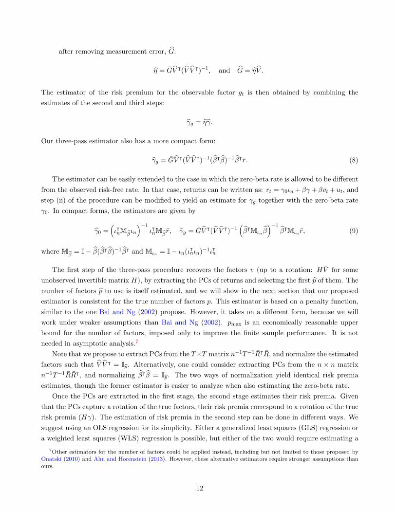
after removing measurement error, G:
η = GV ᵀ(V V ᵀ)−1, and G = ηV .
The estimator of the risk premium for the observable factor gt is then obtained by combining the
estimates of the second and third steps:
γg = ηγ.
Our three-pass estimator also has a more compact form:
γg = GV ᵀ(V V ᵀ)−1(βᵀβ)−1βᵀr. (8)
The estimator can be easily extended to the case in which the zero-beta rate is allowed to be different
from the observed risk-free rate. In that case, returns can be written as: rt = γ0ιn + βγ + βvt + ut, and
step (ii) of the procedure can be modified to yield an estimate for γg together with the zero-beta rate
γ0. In compact forms, the estimators are given by
γ0 =(ιᵀnMβ
ιn
)−1ιᵀnMβ
r, γg = GV ᵀ(V V ᵀ)−1(βᵀMιn β
)−1βᵀMιn r, (9)
where Mβ
= I− β(βᵀβ)−1βᵀ and Mιn = I− ιn(ιᵀnιn)−1ιᵀn.
The first step of the three-pass procedure recovers the factors v (up to a rotation: HV for some
unobserved invertible matrix H), by extracting the PCs of returns and selecting the first p of them. The
number of factors p to use is itself estimated, and we will show in the next section that our proposed
estimator is consistent for the true number of factors p. This estimator is based on a penalty function,
similar to the one Bai and Ng (2002) propose. However, it takes on a different form, because we will
work under weaker assumptions than Bai and Ng (2002). pmax is an economically reasonable upper
bound for the number of factors, imposed only to improve the finite sample performance. It is not
needed in asymptotic analysis.7
Note that we propose to extract PCs from the T×T matrix n−1T−1RᵀR, and normalize the estimated
factors such that V V ᵀ = Ip. Alternatively, one could consider extracting PCs from the n × n matrix
n−1T−1RRᵀ, and normalizing βᵀβ = Ip. The two ways of normalization yield identical risk premia
estimates, though the former estimator is easier to analyze when also estimating the zero-beta rate.
Once the PCs are extracted in the first stage, the second stage estimates their risk premia. Given
that the PCs capture a rotation of the true factors, their risk premia correspond to a rotation of the true
risk premia (Hγ). The estimation of risk premia in the second step can be done in different ways. We
suggest using an OLS regression for its simplicity. Either a generalized least squares (GLS) regression or
a weighted least squares (WLS) regression is possible, but either of the two would require estimating a
7Other estimators for the number of factors could be applied instead, including but not limited to those proposed byOnatski (2010) and Ahn and Horenstein (2013). However, these alternative estimators require stronger assumptions thanours.
12

large number of parameters (e.g., the covariance matrix of ut in GLS or its diagonal elements in WLS).
As it turns out, these estimators will not improve the asymptotic efficiency of the OLS to the first order.
This is different from the standard large T and fixed n case because in our setting the covariance matrix
of ut only matters at the order of Op(n−1 + T−1), whereas the leading term of γg is Op(n
−1/2 + T−1/2).
The third step is a new addition to the standard two-pass procedure. It is critical because it
translates the uninterpretable risk premia of latent factors to those of factors the economic theory
predicts. This step also removes the effect of measurement error, which the standard approaches cannot
accomplish. Even though gt can be multi-dimensional, the estimation for each observable factor is
separate. Estimating the risk premium for one factor does not affect the estimation for the others at
all, another important property of our estimator.
To sum up, our estimator uses PCA to recover factors vt up to a rotation H; it estimates their risk
premia (Hγ) in the second step; it estimates the loading of gt onto the rotated factors (ηH−1) in the
third step; finally, it combines the two to produce a consistent estimator for ηH−1Hγ = γg, where this
last equality is a consequence of the invariance result we derived above.
3.4 Alternative Interpretations
In Section 2 we have discussed how, in general, the two-pass regressions and the mimicking-portfolio
estimators tend to give different estimates, even when the model is correctly specified. As it turns out,
our three-pass estimator can be interpreted both as an extension of the two-pass regressions and as an
extension of the mimicking-portfolio estimator. In this section, we discuss how our estimator brings
together these two different approaches.
Two-pass regression interpretation. The two-pass interpretation of our results derives directly
from the rotation-invariance of risk premia. To begin, suppose that we know the entire model, equations
(1) and (2). Also, suppose for simplicity that gt is only one factor (d = 1; the results extend to any d),
and there is no measurement error.
We now construct a specific rotation of this model in which the factor gt appears as the first of the
p factors, together with p− 1 additional “control” factors. To do so, construct a matrix H in which the
first row is η, and the remaining p− 1 rows are arbitrary (with the only condition that the resulting H
is full rank). The factors of the rotated model are Hvt; since η is the first row of H, the first factor in
this rotation is ηvt, which is just gt (see equation (2)). Similarly, the risk premia of the rotated factors
are Hγ, and the risk premium of the first factor, gt, is ηγ, again because the first row of H is η.
Consider now applying a two-pass cross-sectional regression in this particular rotation, assuming
that all the rotated factors Hvt are observed. Given that the model is correctly specified, the two-pass
regression will recover all the risk premia Hγ: therefore, it will also recover ηγ as the risk premium for
gt. But this result holds for any matrix H where the first row is η, independently of the other rows
of H. This implies that a two-pass estimation of a model where gt appears with p− 1 arbitrary linear
combinations of vt will deliver the correct estimate for the risk premium of gt independently of how the
remaining p − 1 “controls” are rotated. The only requirement is that H is invertible: that is, that gt
together with the controls spans the same space as the original factors vt.
13

Given this result, we can interpret our three-pass estimator as a factor-augmented cross-sectional
regression estimator. Step (i) uses PCA to extract a rotation of the original factors vt. Step (iii) removes
measurement error from gt and identifies η: this tells us how to rotate the estimated model so that gt
appears as the first factor. We can then construct a rotated model with gt together with p − 1 PCs
as controls. Risk premia for this model are estimated via cross-sectional regressions (step (ii)), that
will then deliver a risk premium of ηγ for gt. While this cross-sectional regression interpretation of
the estimator inverts the ordering of steps (ii) and (iii) of our procedure, it gives numerically identical
results.
Mimicking-portfolio interpretation. Our three-pass procedure can be also interpreted as a
mimicking-portfolio estimator, in which the principal components themselves are the portfolios on which
gt is projected. This is an ideal choice of portfolios that ensures that the estimator is consistent.
Suppose that, out of the universe of test assets, we construct p portfolios on which we project gt.
We refer to w as the n× p matrix of portfolio weights that are used to construct these portfolios of rt: so
rt = wᵀrt. In Section 2.2 we showed that in general the mimicking-portfolio estimator is not consistent.
That said, it can be consistent if the returns of the portfolios on which gt is projected (rt) satisfy certain
requirements. In turn, it means that w needs to be chosen carefully so that the mimicking-portfolio
estimator that uses these p portfolios,
γMPg = ηΣvβᵀ(Σr)−1βγ + Σz,u(Σr)−1βγ (10)
actually converges to γg = ηγ.
We now derive a novel property of mimicking-portfolio estimators (not studied in the existing litera-
ture, to the best of our knowledge) that helps us choose w appropriately when the number of test assets
n is large. In particular, we prove in Proposition 1 of Appendix B.1 that the bias of the mimicking-
portfolio estimator (equation 10) disappears as n→∞, as long as the portfolios on which to project gt
are constructed by choosing w equal to β or some full-rank rotation of it.
Intuitively, this choice of w is guaranteed to achieve asymptotically the two criteria highlighted
in Section 2.2: these portfolios manage to average out idiosyncratic errors, while maintaining their
exposure to the factors. The second part is important. Many portfolios can average out idiosyncratic
errors, but they might also average out exposures to certain factors, in which case the omitted variable
bias discussed in this paper would bias the estimates.
Our three-pass method corresponds exactly to a mimicking-portfolio estimator where the portfolios
onto which gt is projected are constructed using a particular choice for w: β(βᵀβ)−1, that is, a full-rank
rotation of the estimated β. The resulting portfolio returns are exactly the PCs in step (i) of our
procedure, i.e., V = (βᵀβ)−1βᵀR. In addition, these portfolios are (when n is large) free of idiosyncratic
error. Step (iii) projects gt onto these portfolios, thus identifying the weights of the mimicking portfolio,
η. Our estimator of the risk premium of gt is then obtained by multiplying the portfolio weights η by
the risk premia of these portfolios (γ) obtained in Step (ii).
Interestingly, Proposition 1 also suggests that another valid choice of w would be the identity matrix.
Therefore, the mimicking-portfolio estimator would also be unbiased if the factor is projected onto the
14

entire universe of potential test assets rt, as opposed to a subset rt, again as long as n→∞. Intuitively,
when gt is projected onto a larger and larger set of test assets, the mimicking portfolio will diversify the
idiosyncratic errors while at the same time spanning the factor space, thus reducing the bias. However,
as n → ∞, the mimicking-portfolio estimator becomes increasingly inefficient, as the number of right-
hand-side regressors increases; when n is larger than T , it actually becomes infeasible. Our three-pass
procedure can therefore be interpreted as a regularized mimicking-portfolio estimator that exploits the
benefits in terms of bias reduction that occur when n→∞, but preserves feasibility and efficiency via
principal component regressions.
To sum up, in standard cases with fixed n, the two-pass cross-sectional regression and mimicking-
portfolio approaches tend to give different answers about the risk premium of a factor gt. Our three-pass
estimator represents the convergence of these two approaches that occurs when PCs are used to span
the space of a large number of test assets.
4 Asymptotic Theory
In this section, we present the large sample distribution of our estimator as n, T → ∞. Our results
hold under the same or even weaker assumptions compared to those in Bai (2003). This is because our
goals are different. Our main target is ηγ, instead of the asymptotic distributions of factors and their
loadings.
4.1 Determining the Number of Factors
Theorem 1. Under Assumptions A.1, A.2, A.4 – A.7, and suppose that as n, T → ∞, φ(n, T ) → 0,
and φ(n, T )/(n−1/2 + T−1/2)→∞, we have pp−→ p.
By a simple conditioning argument, we can assume that p = p when developing the limiting dis-
tributions of the estimators, see Bai (2003). In the remainder of the section, we assume p = p. Even
though consistency cannot guarantee the recovery of the true number of factors in any finite sample,
our derivation in Section 4.5 shows that as long as p ≤ p ≤ K for some finite K, we can estimate the
parameters Γ consistently.
A notable assumption behind is the so-called pervasive condition for a factor model, i.e., Assumption
A.6. It requires the factors to be sufficiently strong that most assets have non-negligible exposures.
This is a key identification condition, which dictates that the eigenvalues corresponding to the factor
components of the return covariance matrix grow rapidly at a rate n, so that as n increases they can be
separated from the idiosyncratic component whose eigenvalues grow at a lower rate. The pervasiveness
assumption precludes weak but priced latent factors. We defer a more detailed discussion of this to
Section 5.6.3.
4.2 Limiting Distribution of the Risk Premia Estimator
We now present the main theorem of the paper – the asymptotic distribution of the estimator γg, which
naturally needs more assumptions reported in detail in Appendix A.
15

Theorem 2. Under Assumptions A.1, A.2, A.4 – A.11, and suppose pp−→ p, then as n, T → ∞, we
have
γ −Hγ = Hv +Op(n−1 + T−1), η − ηH−1 = T−1ZV ᵀHᵀ +Op(n
−1 + T−1),
for some matrix H that is invertible with probability approaching 1. Moreover, if T 1/2n−1 → 0,
T 1/2 (γg − ηγ)L−→ N (0,Φ) ,
where Φ is given by
Φ =(γᵀ (Σv)−1 ⊗ Id
)Π11
((Σv)−1 γ ⊗ Id
)+(γᵀ (Σv)−1 ⊗ Id
)Π12η
ᵀ
+ ηΠ21
((Σv)−1 γ ⊗ Id
)+ ηΠ22η
ᵀ. (11)
Remarkably, the asymptotic covariance matrix does not depend on the covariance matrix of the
residual ut or the estimation error of β. Their impact on the asymptotic variance is of higher orders.
Therefore, for the inference on the risk premium of gt, there is no need to estimate the large covariance
matrix of ut. This also implies that the usual GLS or WLS estimator would not improve the efficiency
of the OLS estimator to the first order.8
4.3 Allowing for Pricing Errors and Zero-beta Rate
Now we extend the above results to a more general setting, in which the zero-beta rate is unrestricted,
and in which mispricing is allowed for in the model. This case represents the most general setting in
which our estimator is consistent.
Suppose the cross-section of asset returns rt follows
rt = α+ ιnγ0 + βγ + βvt + ut, (12)
where the cross-sectional pricing error α is i.i.d., independent of β, u and v, with mean 0, standard
deviation σα > 0, and a finite fourth moment.
There is a large body of literature on testing the APT by exploring the deviation of α from 0,
including Connor and Korajczyk (1988), Gibbons et al. (1989), MacKinlay and Richardson (1991), and
more recently, Pesaran and Yamagata (2012) and Fan et al. (2015). This is, however, not the focus
of this paper. Empirically, the pricing errors may exist for many reasons such as limits to arbitrage,
transaction costs, market inefficiency, and so on, so that it is important to allow for a misspecified
linear factor model. Gospodinov et al. (2014) and Kan et al. (2013) also consider this type of model
misspecification in their two-pass cross-sectional regression setting.
In this case, we employ the alternative estimator (9).
8Indeed, we can show that our estimator is asymptotically equivalent to the infeasible GLS.
16

Theorem 3. Under Assumptions A.2, A.4 – A.14, and suppose pp−→ p, then as n, T →∞, we have
n1/2 (γ0 − γ0)L−→ N
(0,(
1− βᵀ0(Σβ)−1β0
)−1(σα)2
),(
T−1Φ + n−1Υ)−1/2
(γg − ηγ)L−→ N (0, Id) ,
where the asymptotic covariance matrices Φ is given by (11), and Υ is defined by
Υ =(σα)2η(
Σβ − β0βᵀ0
)−1ηᵀ.
Unlike the CLT in Theorem 2, the result of Theorem 3 does not impose any restrictions on the
relative rates of n and T . Also, the above analysis assumes that the factor loading β is uncorrelated
with the pricing error α, which means that the mispricing is not related to risk exposures. In fact,
even if they were correlated, our estimator would instead converge to the “pseudo-true” parameter
η(γ + plimn→∞(βᵀMιnβ)−1βᵀα
), which is difficult to interpret, see, e.g., Kan et al. (2013).
4.4 Goodness-of-Fit Measures
To measure the goodness-of-fit in the cross-section of expected returns, we define the usual (population)
cross-sectional R2 for the latent factors in (12):
R2v =
γᵀ(Σβ − β0βᵀ0)γ
(σα)2 + γᵀ(Σβ − β0βᵀ0)γ
.
To measure the signal-to-noise ratio of each observable factor, we define the time-series R2 for each
observable factor g (1× T ) in the time-series regression of gt on the latent factors:
R2g =
ηΣvηᵀ
ηΣvηᵀ + Σz, where η is a 1× p vector.
To calculate these measures in sample, we use
R2v =
rᵀMιn β(βᵀMιn β)−1βᵀMιn r
rᵀMιn rand R2
g =ηV V ᵀηᵀ
GGᵀ, respectively,
where G = g − g is a 1 × T vector. We can consistently estimate the cross-sectional R2 for the latent
factors as well as the time-series R2 for each observable factor.
Theorem 4. Under Assumptions A.2, and A.4 – A.14, and suppose pp−→ p, then as n, T → ∞, we
have
R2v
p−→ R2v and R2
gp−→ R2
g.
17

4.5 Robustness to the Choice of p
Although p is a consistent estimator of p, it is possible that in a finite sample p 6= p. In fact, without
a consistent estimator of p, as long as our choice, denoted by p, is greater than or equal to p, the
estimators based on p, denoted by γ0 and γg, are consistent, as the next theorem shows.
Theorem 5. Suppose Assumptions A.2, and A.4 – A.14 hold. In addition, assume that ut is i.i.d.
N(0, (σu)2In
), independent of zt and vt. If p ≥ p and p ≤ K as n/T → c ∈ (0,∞), then γ0 and γg are
consistent estimators of γ0 and ηγ, and it holds that
γ0 − γ0 = Op(n−1/2), γg − γg = Op(n
−1/2).
The above theorem establishes the desired robustness to the inclusion of “noise” factors.9 While we
cannot establish its asymptotic distribution, simulation exercises suggest that the differences between
the asymptotic variances of γg and γg are tiny. This is also the case for our empirical study.
4.6 Asymptotic Variances Estimation
We develop consistent estimators of the asymptotic covariances in Theorem 8. The case for estimator
(8) in Theorem 2 is simpler. We can estimate them for inference on risk premia using:
Φ =(γᵀ(Σv)−1 ⊗ Id
)Π11
((Σv)−1γ ⊗ Id
)+(γᵀ(Σv)−1 ⊗ Id
)Π12η
ᵀ + ηΠ21
((Σv)−1γ ⊗ Id
)+ ηΠ22η
ᵀ,
Υ =σα2η(
Σβ − β0βᵀ0
)−1ηᵀ,
where Π11, Π12, Π22, are the HAC-type estimators of Newey and West (1987), defined as:
Π11 =1
T
T∑t=1
vec(ztvᵀt )vec(ztv
ᵀt )ᵀ
+1
T
q∑m=1
T∑t=m+1
(1− m
q + 1
)(vec(zt−mv
ᵀt−m)vec(ztv
ᵀt )ᵀ + vec(ztv
ᵀt )vec(zt−mv
ᵀt−m)ᵀ
),
Π12 =1
T
T∑t=1
vec(ztvᵀt )vᵀt +
1
T
q∑m=1
T∑t=m+1
(1− m
q + 1
)(vec(zt−mv
ᵀt−m)vᵀt + vec(ztv
ᵀt )vᵀt−m
),
Π22 =1
T
T∑t=1
vtvᵀt +
1
T
q∑m=1
T∑t=m+1
(1− m
q + 1
)(vt−mv
ᵀt + vtv
ᵀt−m
),
and
Z =G− ηV , Σβ = n−1βᵀβ, Σv = T−1V V ᵀ, β0 = n−1βᵀιn, σα2
= n−1∥∥∥r − (ιn : β)Γ
∥∥∥2
F,
9To prove this result, we need much stronger assumptions on ut. This is because the proof relies on the use of randommatrix theory to analyze the eigenvalues and eigenvectors of large sample covariance matrices. The i.i.d. assumption istypically need in such scenarios.
18

γ =(βᵀMιn β
)−1βᵀMιn r, Γ = (γ0 : γᵀ)ᵀ,
with q →∞, q(T−1/4 + n−1/4)→ 0, as n, T →∞.
To prove the validity of these estimators, we need additional assumptions, because the estimands
are more complicated than the parameters we estimate.
Theorem 6. Under Assumptions A.2, and A.4 – A.16, and suppose that pp−→ p, then as n, T →∞,
n−3T → 0, q(T−1/4 + n−1/4)→ 0, Φp−→ Φ and Υ
p−→ Υ.
4.7 Testing the Strength of an Observed Factor
As discussed in the introduction, a recent literature has explored the potential problem in inference on
risk premia in the presence of weak factors (factors that are only weakly reflected in the cross-section of
test assets). Our methodology is in fact robust to the case in which observable factors gt are weak. In
particular, whether gt is strong or weak can be captured by the signal-to-noise ratio of its relationship
with the underlying factors vt (from equation (2)). If either η = 0 (gt is not a priced factor) or the
factor is very noisy (measurement error zt dominates the gt variation) then gt will be weak, and returns
exposures to gt will be small.
Our procedure estimates equation (2) in the third pass and is therefore able to detect whether an
observable proxy gt has zero or low exposures to the fundamental factors (η is small) or whether it is
noisy (zt is large), and corrects for it when estimating the risk premium. The R2 of that regression
reveals how noisy g is, which, as we report in our empirical analysis, varies substantially across factor
proxies. In this section, we provide a Wald test for the null hypothesis that a factor g is weak.
Without loss of generality, it is sufficient to consider the d = 1 case. To do so, we formulate the
hypotheses H0 : η = 0 vs H1 : η 6= 0, and construct a Wald Test. Our test statistic is given by
W = T η(
Σ−1v Π11Σ−1
v
)−1ηᵀ,
where Π11 and Σv are constructed in Section 4.6.
The next theorem establishes the desired size control and the consistency of the test.
Theorem 7. Suppose d = 1 and pp−→ p. Under Assumptions A.2, and A.4 – A.16, and as n, T →∞,
n−2T → 0, q(T−1/4 + n−1/4)→ 0, we have
limn,T→∞
P(W > χ2
p(1− α0)|H0
)= α0, and lim
n,T→∞P(W > χ2
p(1− α0)|H1
)= 1,
where χ2p(1− α0) is the (1− α0)-quantile of the chi-squared distribution with p degree of freedom.
Our assumptions that the latent factors are pervasive, while observable factors can potentially be
weak, are not in conflict with existing empirical evidence. It is known from the literature (e.g., Bernanke
and Kuttner (2005) and Lucca and Moench (2015)) that the stock market and the bond market strongly
react to Federal Reserve and Government policies and that macroeconomic risks affect equity premia;
fundamental macroeconomic shocks seem to be pervasive. At the same time, we do not observe all
19

fundamental economic shocks directly, and have instead to rely on observable proxies; these are well
known to be weak in some cases, like for example industrial production (see Gospodinov et al. (2014)
and Bryzgalova (2015)).
5 Empirical Analysis
In this section we apply our three-pass methodology to the data. We estimate the risk premia of several
factors, both traded and not traded, and show how our results differ from those obtained using standard
two-pass cross-sectional regressions and mimicking portfolios.
5.1 Data
We conduct our empirical analysis on a large set of standard portfolios of U.S. equities, testing several
asset pricing models that have focused on risk premia in equity markets. We target U.S. equities
because of their better data quality and because they are available for a long time period. However,
our methodology could be applied to any country or asset class.
We include in our analysis 202 portfolios: 25 portfolios sorted by size and book-to-market ratio, 17
industry portfolios, 25 portfolios sorted by operating profitability and investment, 25 portfolios sorted
by size and variance, 35 portfolios sorted by size and net issuance, 25 portfolios sorted by size and
accruals, 25 portfolios sorted by size and beta, and 25 portfolio sorted by size and momentum. This set
of portfolios captures a vast cross section of anomalies and exposures to different factors; at the same
time, they are easily available on Kenneth French’s website, and therefore represent a natural starting
point to illustrate our methodology.10
Although some of these portfolio returns have been available since 1926, we conduct most of our
analysis on the period from July of 1963 to December of 2015 (630 months), for which all of the returns
are available. We perform the analysis at the monthly frequency, and work with factors that are available
at the monthly frequency.
Although the asset-pricing literature has proposed an extremely large number of factors (McLean
and Pontiff (2015); Harvey et al. (2016)), we focus here on a few representative ones. Recall that
the observable factors gt in the three-pass methodology can be either an individual factor or groups
of factors. We consider here both cases to illustrate the methodology; importantly, the risk premia
estimates for any factors using our three-pass methodology do not depend on whether other factors are
included in gt (though this does matter for the two-pass cross-sectional estimator). Here is a list of
models and corresponding observable factors gt we include in our analysis:11
1. Capital Asset Pricing Model (CAPM ): the value-weighted market return, constructed from the
Center for Research in Security Prices (CRSP) for all stocks listed on the NYSE, AMEX, or
10See the description of all portfolio construction on Kenneth French’s website: http://mba.tuck.dartmouth.edu/
pages/faculty/ken.french/data_library.html.11Factor time series for models 1-4 are obtained from Kenneth French’s website; for models 5-6, from AQR’s website;
for model 7, from the Federal Reserve Bank of St. Louis; for model 8, from Sydney Ludvigson’s website; for model 9,from Lubos Pastor’s website; for model 10, from Bryan Kelly’s website; for model 11, from the various sources indicatedin Novy-Marx (2014); for model 12, from Toby Moskowitz’s website.
20

NASDAQ.
2. Fama-French three factors (FF3 ): in addition to the market return, the model includes SMB
(size) and HML (value).
3. Carhart’s four-factor model (FF4 ) that adds a momentum factor (MOM) to FF3.
4. Fama-French five-factor model (FF5 ), from Fama and French (2015). The model adds to FF3
RMW (operating profitability) and CMA (investment).12
5. Betting-against-beta factor (BAB) from Frazzini and Pedersen (2014).
6. Quality-minus-junk factor (QMJ ) from Asness et al. (2013).
7. Industrial production growth (IP). Industrial production is a macroeconomic factor available for
the entire sample period at the monthly frequency. We use AR(1) innovations as the factor.
8. The first three principal components of 279 macro-finance variables constructed by Ludvigson and
Ng (2009) (LN ), also available at the monthly frequency. We estimate a VAR(1) with those three
principal components, and use innovations as factors.
9. The liquidity factor from Pastor and Stambaugh (2003).
10. Two intermediary capital factors, one from He et al. (2016) and one from Adrian et al. (2014).
11. Four factors from Novy-Marx (2014): high monthly temperature in Manhattan, global land sur-
face temperature anomaly, quasiperiodic Pacific Ocean temperature anomaly (El Nino), and the
number of sunspots.13
12. Two consumption-based factors from Malloy et al. (2009). They include both an aggregate con-
sumption series and a stockholder’s consumption series.
5.2 Factors from the Large Panel of Returns
The first step for estimating the observable factor risk premia is to determine the dimension of the
latent factor model, p. Figure 1 (left panel) reports the first eight eigenvalues of the covariance matrix
of returns for our panel of 202 portfolios. As typical for large panels, the first eigenvalue tends to be
much larger than the others, so on the right panel we plot the eigenvalues excluding the first one. We
observe a noticeable decrease in the eigenvalues up to four factors, suggesting p = 4. This is also the
number suggested by our estimator. As discussed in Section 4, our analysis is consistent as long as the
number of factors p is at least as large as the true dimension p; to show the robustness of our results,
12We have also explored the four-factor model of Hou et al. (2015), which includes the market return, ME (size), IA(investment), ROE (profitability). Results are qualitatively and quantitatively similar to the FF5.
13These time series have been proposed by Novy-Marx (2014) as examples of variables that appear to predict returnsin standard predictive regressions, but whose economic link to the stock market seems weak. We use AR(1) innovationsin these series as factors and test whether our procedure identifies the weak link to the economy, and reveals the series asweak or unpriced in the cross-section of returns.
21
we report the estimates separately using four, five, and six factors. The analysis is robust to using more
factors.
The model with four PCs has a cross-sectional R2 of 65%, indicating that it accounts for a significant
fraction of the cross-sectional variation in expected returns for the 202 test portfolios, but leaving some
unexplained variation. This number is comparable with the 73% cross-sectional R2 one obtains using
the FF3 model on the cross-section of 25 portfolios sorted by size and book-to-market, yet, we obtain
it for a cross-section eight times as large, and using a model with just one more factor. We report
in Figure 2 the actual and predicted expected excess returns for the model. Each panel of the figure
highlights one of the eight test-asset groups that comprise our total of 202 portfolios. The fit is better
for some groups of assets than others, but overall the factor model performs relatively well.
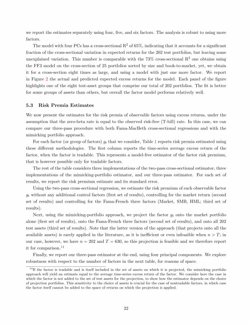
5.3 Risk Premia Estimates
We now present the estimates for the risk premia of observable factors using excess returns, under the
assumption that the zero-beta rate is equal to the observed risk-free (T-bill) rate. In this case, we can
compare our three-pass procedure with both Fama-MacBeth cross-sectional regressions and with the
mimicking portfolio approach.
For each factor (or group of factors) gt that we consider, Table 1 reports risk premia estimated using
these different methodologies. The first column reports the time-series average excess return of the
factor, when the factor is tradable. This represents a model-free estimator of the factor risk premium,
that is however possible only for tradable factors.
The rest of the table considers three implementations of the two-pass cross-sectional estimator, three
implementations of the mimicking-portfolio estimator, and our three-pass estimator. For each set of
results, we report the risk premium estimate and its standard error.
Using the two-pass cross-sectional regression, we estimate the risk premium of each observable factor
gt without any additional control factors (first set of results), controlling for the market return (second
set of results) and controlling for the Fama-French three factors (Market, SMB, HML; third set of
results).
Next, using the mimicking-portfolio approach, we project the factor gt onto the market portfolio
alone (first set of results), onto the Fama-French three factors (second set of results), and onto all 202
test assets (third set of results). Note that the latter version of the approach (that projects onto all the
available assets) is rarely applied in the literature, as it is inefficient or even infeasible when n > T ; in
our case, however, we have n = 202 and T = 630, so this projection is feasible and we therefore report
it for comparison.14
Finally, we report our three-pass estimator at the end, using four principal components. We explore
robustness with respect to the number of factors in the next table, for reasons of space.
14If the factor is tradable and is itself included in the set of assets on which it is projected, the mimicking portfolioapproach will yield an estimate equal to the average time-series excess return of the factor. We consider here the case inwhich the factor is not added to the set of test assets for the projection, to show how the estimator depends on the choiceof projection portfolios. This sensitivity to the choice of assets is crucial for the case of nontradable factors, in which casethe factor itself cannot be added to the space of returns on which the projection is applied.
22
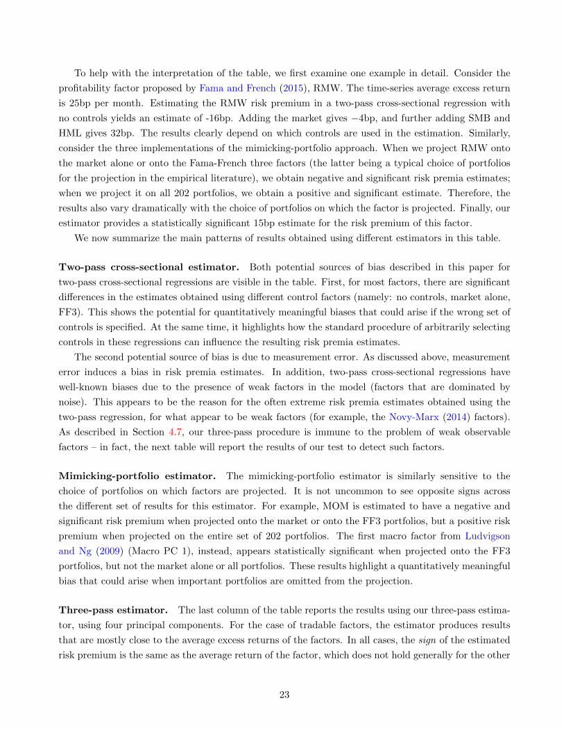
To help with the interpretation of the table, we first examine one example in detail. Consider the
profitability factor proposed by Fama and French (2015), RMW. The time-series average excess return
is 25bp per month. Estimating the RMW risk premium in a two-pass cross-sectional regression with
no controls yields an estimate of -16bp. Adding the market gives −4bp, and further adding SMB and
HML gives 32bp. The results clearly depend on which controls are used in the estimation. Similarly,
consider the three implementations of the mimicking-portfolio approach. When we project RMW onto
the market alone or onto the Fama-French three factors (the latter being a typical choice of portfolios
for the projection in the empirical literature), we obtain negative and significant risk premia estimates;
when we project it on all 202 portfolios, we obtain a positive and significant estimate. Therefore, the
results also vary dramatically with the choice of portfolios on which the factor is projected. Finally, our
estimator provides a statistically significant 15bp estimate for the risk premium of this factor.
We now summarize the main patterns of results obtained using different estimators in this table.
Two-pass cross-sectional estimator. Both potential sources of bias described in this paper for
two-pass cross-sectional regressions are visible in the table. First, for most factors, there are significant
differences in the estimates obtained using different control factors (namely: no controls, market alone,
FF3). This shows the potential for quantitatively meaningful biases that could arise if the wrong set of
controls is specified. At the same time, it highlights how the standard procedure of arbitrarily selecting
controls in these regressions can influence the resulting risk premia estimates.
The second potential source of bias is due to measurement error. As discussed above, measurement
error induces a bias in risk premia estimates. In addition, two-pass cross-sectional regressions have
well-known biases due to the presence of weak factors in the model (factors that are dominated by
noise). This appears to be the reason for the often extreme risk premia estimates obtained using the
two-pass regression, for what appear to be weak factors (for example, the Novy-Marx (2014) factors).
As described in Section 4.7, our three-pass procedure is immune to the problem of weak observable
factors – in fact, the next table will report the results of our test to detect such factors.
Mimicking-portfolio estimator. The mimicking-portfolio estimator is similarly sensitive to the
choice of portfolios on which factors are projected. It is not uncommon to see opposite signs across
the different set of results for this estimator. For example, MOM is estimated to have a negative and
significant risk premium when projected onto the market or onto the FF3 portfolios, but a positive risk
premium when projected on the entire set of 202 portfolios. The first macro factor from Ludvigson
and Ng (2009) (Macro PC 1), instead, appears statistically significant when projected onto the FF3
portfolios, but not the market alone or all portfolios. These results highlight a quantitatively meaningful
bias that could arise when important portfolios are omitted from the projection.
Three-pass estimator. The last column of the table reports the results using our three-pass estima-
tor, using four principal components. For the case of tradable factors, the estimator produces results
that are mostly close to the average excess returns of the factors. In all cases, the sign of the estimated
risk premium is the same as the average return of the factor, which does not hold generally for the other
23

estimators. For example, it estimates a market risk premium of around 50bp (exactly in line with the
average market excess return) and a momentum risk premium of 77bp.
The three-pass procedure finds several nontradable factor risk premia economically and statistically
significant: the liquidity factor of Pastor and Stambaugh (2003), both intermediary factors of He et al.
(2016) and Adrian et al. (2014), the first macro PC from Ludvigson and Ng (2009), and also stockholders’
consumption growth from Malloy et al. (2009). Nonetheless, several other nontradable factors do not
appear to have statistically significant risk premia, for example the Novy-Marx (2014) factors or IP
growth.
To conclude, for the tradable factors we study, the three-pass estimator produces results that are
broadly consistent with the time-series average returns of those factors; for the nontradable factors,
they produce estimates that have economically reasonable magnitudes. The results are often noticeably
different from those produced by the other estimators, which vary substantially across implementations.
Allowing for a unconstrained zero-beta rate. Table 2 shows the results produced by our more
general estimator (9), that allows the zero-beta rate to be different from the T-bill rate.15 We do
not report the mimicking portfolio results here because that estimation approach does not allow for
an unconstrained zero-beta rate. Instead, we report in this table our three-pass results for different
numbers of PCs, from 4 to 6. Also, we do not report the estimates for the zero-beta rate for reasons
of space. For the three-pass procedure, they are consistently around 0.55% per month (close to the
average T-bill return of 0.4% per month).16 For the two-pass regressions, they are in the vast majority
of cases significantly above 1% per month.
The results with the unconstrained zero-beta rate are mostly similar to those presented in the
previous table, but there are some additional noteworthy results. First, the table shows that risk
premia estimates using the three-pass method are very robust to the number of PCs used (from 4 to
6). For example, for the liquidity factor we estimate a risk premium of 26bp with 4 and 5 factors, and
25bp with 6 factors. Similar results hold for all factors, both tradable and nontradable.
Second, the table also reports the R2 of the time-series regression of each observed factor gt onto the
p latent factors; we refer to this as R2g. R2
g will be lower than 100% when measurement error is present
in the factor gt. In the data, we find great heterogeneity among factors in terms of their measurement
error. For some of them (like the market or SMB) this R2 is extremely high, suggesting that the factor
is measured essentially without error. For many other factors, and especially so for nontradable factors,
the R2g is much lower (for IP, for example, it is below 1%), indicating that these factors are dominated
by noise. We highlight this point in Figure 3, which shows the time series of cumulated innovations
in the original and cleaned (i.e., fitted) factors, for a few of them. The figures provide a graphical
representation of the extent to which the PCs of returns capture the variation in each factor. While
for many of the tradable factors the original and cleaned factors track each other closely, for others the
15The inference based on Theorem 3 in this case is also robust to the presence of pricing errors (alphas) that satisfy ourassumptions.
16Recall that in the case of the three-pass procedure, the estimate of the zero-beta rate, obtained at step (ii), does notdepend on the factor gt.
24

cleaned factor displays much lower variation than the original factor: the difference is the measurement
error that our procedure has eliminated.
Finally, the last column of the table also reports the p-value for the test of the null that each factor
gt is weak, described in Section 4.7.17 A rejection of the null indicates that gt is a strong factor for the
cross-section of test portfolios. For several – but not all – of the nontradable factors we fail to reject
that the factor is weak.
The zero-beta rate and the sign of the market risk premium. A well-known result in the
empirical asset pricing literature is that market risk premia are estimated to be negative in standard
two-pass regressions with an unrestricted zero-beta rate. This happens in our dataset as well. The
two-pass estimators of the market risk premium yield a zero-beta rate estimate of around 125bp per
month (not reported in the table) and a market risk premium of -20bp to -57bp per month, depending
on the specification (first row of Table 2).
If this puzzling result is due to the omission of important controls (measurement error bias is
unlikely because of the large R2g), we expect our three-pass estimator to correct for it. Indeed the
three-pass procedure lowers the estimated zero-beta rate (to 55bp per month) and produces a positive
and significant estimate of the market risk premium (37bp), as the right side of the first row shows.
We can further investigate the relationship between market beta and expected returns after control-
ling for the explanatory power of the omitted factors using a residual regression approach.18 Figure 4
plots the expected return vs. market beta, after partialing out the component explained by the other
factors. The left panel uses the standard two-pass estimator for the market risk premium in the FF3
model, whereas the right panel uses our three-pass methodology. The solid red line in each graph corre-
sponds to the slope estimated from the historical average return of the market, whereas the dashed line
corresponds to the fitted line, using the cross-sectional estimate of the slope. Given that the market is
a tradable factor, if the model is correctly specified, the two lines should overlap.
This is clearly not the case for the two-pass cross-sectional regression (left panel). However, the
right panel of the figure shows that indeed, once the omitted factors are accounted for, there is a clear
positive relationship between market beta and expected returns, and the slope is close to the average
excess return of the market portfolio. Overall, the fact that the market risk premium significantly
changes sign depending on whether we control for omitted factors serves as a strong warning that
omitting factors could have important effects on our statistical and economic conclusions about the
pricing of risks.
17To be more conservative, we use p = 6 for this test, corresponding to the rightmost set of results in the table, butresults are quite similar for all values of p.
18Recall that the estimate of the market risk premium using cross-sectional methods is the slope of a multivariateregression of average returns onto the betas of returns with respect to the market and the control factors. It is well knownthat the slope of any multivariate regression with respect to a specific variable (in this case, the market beta) can be alsoobtained by first separately regressing the outcome variable (average returns) and the regressor of interest (market beta)on the remaining regressors (the betas with respect to the other factors), and in a second stage regressing the residuals ofthe two regressions against each other. In this way, we can first partial out the component of the cross-section of expectedreturns and of market betas explained by the control factors, and then study the univariate relation between the residuals.
25

5.4 Observable and Unobservable Factors
The core of our estimation methodology is the link between the observable factors gt and the unobserv-
able factors vt, through Equation (2). In particular, η represents the loadings of gt onto the p PCs, and
therefore reveals the exposures of the observable factors to the latent factors extracted by PCA.
In Table 3 we decompose the variance of gt explained by the set of PC factors into the parts at-
tributable to exposure to each individual PC factor (which is possible because PC factors are orthogonal
to each other). Each row of the table sums up to 100%. This allows us to highlight which latent factors
are most responsible for the variation of each observable factor. Note that the PC factors are ordered
by their eigenvalues (largest to smallest).
The first row shows that the market return loads mostly onto the first PC (i.e., on the factor with
the largest eigenvalue). This is expected because the market represents the largest source of common
variation across assets. The other observable factors show interesting variation in their exposure to the
PCs. For example, SMB loads on both the first and second factors, HML mostly on the third one, and
MOM mostly on the fourth one. RMW loads substantially on at least four factors (including the sixth
one), and CMA loads mostly on the same factor as HML. However, CMA and HML are still strongly
distinguished by a differential exposure to the other factors.
Macro factors load onto the PCs in nontrivial ways. IP is mostly exposed to the fourth and sixth
factors. The consumption factor loads mostly on the first two latent factors, whereas the stockholder
consumption factor loads most strongly on the fifth one. The Novy-Marx (2014) factors and the Lud-
vigson and Ng (2009) factors are exposed to many risk sources.
Finally, both the liquidity factor of Pastor and Stambaugh (2003) and the intermediary factor of He
et al. (2016) are strongly exposed to the first latent factor.
A caveat about these results is that the PCs cannot be interpreted as “fundamental” factors, but
rather as an unknown rotation of them. So this decomposition cannot be viewed as linking the observable
factors to any interpretable latent factors. Rather, it simply shows similarities and differences in the
source of common variation different observable factors are related to.
5.5 Risk Premia across Asset Classes
The main analysis presented in the previous sections has focused on a large cross-section of equity
portfolios, for which a long time series is available. In this section we explore risk premia for the same
factors discussed above as we look instead at non-equity portfolios.
We obtain from Asaf Manela’s website the time series of non-equity portfolio returns used in He
et al. (2016), which in turn collects portfolio data from various sources. The data includes ten maturity-
sorted government bond portfolios, ten corporate bond portfolios sorted on yield spread, six sovereign
bond portfolios, 18 S&P 500 option portfolios sorted on moneyness and maturity, six currency portfolios
sorted on interest rate differentials, six currency portfolios sorted on currency momentum, 24 commodity
futures returns, and 20 CDS portfolios sorted by spread, for a total of 100 non-equity portfolios. Due
to data availability for the non-equity portfolios, the sample covers the period 1970-2012. In addition,
since not all portfolios are available for the entire time period, we estimate the variance and pairwise
26

covariances separately with all available data. While the resulting covariance matrix is not necessarily
positive-definite, it leads to consistent estimates for PCs.
Table 4 reports the results of the risk premia estimation with our three-pass procedure using equity
and non-equity assets. The left panel of the table shows the results using the 202 equity portfolios (as in
our main analysis) over this sample period. The results are qualitatively and quantitatively similar to
our baseline results that use a longer sample. The middle panel of the table uses as test assets the 100
non-equity portfolios together with some equity portfolios (the Fama-French 25 portfolios), whereas the
right panel uses only the non-equity portfolios. We use five principal components in the first two panels
and six in the third (consistent with our estimator for p in this sample), achieving a cross-sectional R2
of 58%, 57%, and 54% respectively.
For many (but not all) factors, the estimates of risk premia over these different groups of test
portfolios are surprisingly stable. For example, the market risk premium is estimated to be positive and
large in the cross-section of non-equity portfolios; similarly, the liquidity factor displays a risk premium
of around 20bp per month in all of these samples, and the same goes for the intermediary capital factors
(significance is a bit reduced in this table relative to the previous tables, because the sample is shorter).
Finally, IP is estimated to have a zero risk premium in every case. So while the risk premia associated
with some factors (like equity momentum or profitability) do not seem to be stable across markets, the
analysis does uncover factors that seem to display consistent risk premia in all markets we study.
These results suggest the existence of common risk factors across different markets. While some
degree of segmentation surely exists across these markets, these results indicate that at least some
aggregate risk factors may be pervasive across many markets and their risk premia are consistent across
them. Unlike FF3 or FF5 for equity markets, there are no well-established models or factors that serve
as a good benchmark across markets. In this case, key to correctly uncovering the risk premium of these
factors is to properly control for the unobservable factors specific to each market, something that our
approach can achieve.
5.6 Robustness and Extensions
In this section we explore the robustness of our main results to the choice of test portfolios, sample
period, and choice of the method to recover the factor space, particularly as it relates to the potential
weakness of factors. We also discuss how to handle time variation in risk premia and risk exposures.
5.6.1 Robustness to the Choice of Test Portfolios
Our main empirical results are obtained using a large set of 202 portfolios, and our methodology is
specifically designed to be used with as many assets as possible, so that all relevant dimensions of risk
will be expressed in the cross section. It is natural, however, to wonder to what extent the results are
affected by the particular selection of test assets.
To investigate this question systematically, we perform the following robustness exercise. From the
202 test portfolios we use in our empirical exercise, we randomly select (without replacement) half of
them, and we re-estimate the risk premia of all observable factors in this subsample. We repeat this
27

exercise 10,000 times, thus obtaining a distribution of risk premia estimates across subsamples of 101
portfolios each, randomly selected.
Figure 5 shows the results for several factors. Note that all panels of the figure report the same
range of risk premia (x axis, between -20bp and 100bp), so that the histograms are easily comparable
across panels. The results are quite heterogeneous across factors. In the top left panel, we see that the
risk premium for the market return is clearly positive in the vast majority of cases (it is below zero only
in a small set of subsamples). At the same time, its exact magnitude varies across subsamples. The top
right panel shows that instead the risk premia of SMB and HML are much more precisely estimated
using our three-pass regression method, and similarly for MOM (middle left panel).
The last three panels show interesting results for non-tradable factors. Confirming the results of
Table 2 and Figure 3, IP is a useless factor, with a risk premium of effectively zero across all subsamples.
On the contrary, liquidity and intermediary capital factors all appear positively priced across subsamples.
Overall, our subsample results show that the conclusions of our empirical analysis are robust to the
selection of the test assets.
5.6.2 Robustness to the Choice of Time Period
A potential concern when working with PCs is the stability of the estimated loadings and factors over
time. The extent to which our risk premia estimates are consistent across time periods is an empirical
question that we explore in this section.
Similarly to the robustness with respect to the test assets, we perform our robustness check with
respect to the sample period by resampling half of the time periods randomly without replacement, and
looking at the variability of the risk premia estimates. Simple resampling in the time series is possible
in our context because of the low serial correlation of returns and factor innovations over time.
Figure 6 shows the results. Both quantitatively and qualitatively, the results are very similar to the
ones in the previous section (where we randomly resampled the cross-section as opposed to the time
series). The results show that all of the main conclusions of our main analysis hold when looking across
subsamples.
While the stability across subsamples may seem surprising, it is useful to note that our risk premia
estimator is not only based on PCA. Instead, a key step is the projection of the factor of interest gt
onto the extracted PCs. So any rotation that makes the extracted factors differ across subsamples will
be entirely offset by a corresponding rotation of the loading of gt onto those factors – resulting in stable
risk premia estimates for the observable factors.
5.6.3 Robustness to the Presence of Weak Latent Factors
For the invariance result to hold, it is essential that the control factors, together with gt, span the
entire factor space. The first step of our three-pass procedure involves using PCA to recover the factor
space. As we discuss in the paper, our procedure works even if the observable factor gt is weak (in fact,
we propose a test for whether gt is weak); however, PCA will not necessarily recover the entire factor
space if the underlying latent factors are weak. In this section we summarize our main theoretical and
28

empirical arguments for using PCA in practice, and propose an additional robustness test to mitigate
the concern that the presence of weak factors may distort our results.
In theory, weak latent factors – unobservable factors for which the dispersion of risk exposures is
small in the cross-section – can affect our estimator because they have low eigenvalues, and PCA might
fail to separate them from noise. However, for weak factors to bias our estimates of risk premia for
observable factors, they also need to have themselves high risk premia, which allows them to explain
a significant portion of the cross-section of average returns. But large risk premia for factors with low
eigenvalues imply high Sharpe ratios. A first theoretical argument in favor of focusing on the PCs with
largest eigenvalues are good-deal bounds, which impose a theoretical upper bound on the potential bias
from weak factors (Kozak et al. (2017) make precisely this argument to support using PCA in this
context).
A second, empirical, argument is that we can easily add additional PCs with lower and lower
eigenvalues, and verify that the risk premia estimates are stable. For example, in Table 2, we explore
the robustness of the results using 4, 5 and 6 factors. These robustness exercises are theoretically
motivated by Theorem 5, which guarantees that adding a few “too many” PCs does not affect the
consistency of our estimator.
A third way to verify that weak latent factors are not driving our empirical results is the comparison
of the risk premia estimated for tradable factors using our three-pass procedure with those obtained
as time-series average of the portfolios’ excess returns. As discussed in previous sections, the two
should be the same if the factor model is correctly specified. Biases due to the presence of weak latent
factors should produce significant differences between the estimates using cross-sectional methods and
the time-series averages.
Finally, we propose here an additional robustness test with respect to the possibility of weak factors,
based on changing the objective function when extracting the statistical factors from the panel of returns.
Recall that the first step towards PCA is to calculate eigenvalues of the covariance matrix of returns,
which equal the variances of the corresponding PCs, and that the constructed factors are eigenvectors
associated with the largest few eigenvalues.
Since weak factors are factors with low eigenvalues, which however explain the cross-section of
returns, we can modify the objective function to account for the contribution to the cross-sectional
variation. That is, rather than finding factors that best explain the time-series comovement of stock
returns, we find factors that strike a balance between explaining the time-series comovement of stock
returns and the cross-sectional variation of expected returns. This alternative objective function was
first proposed by Connor and Korajczyk (1986). It is a convenient reference point because it puts
equal weight on the two components of the objective function – the time-series and the cross-sectional
variation.
As shown in Bai and Ng (2002), our PCA formula given in (7) is the solution to the following
optimization problem:
minβ,V
n−1T−1∥∥R− βV ∥∥2
F, subject to T−1V V ᵀ = Ip,
29

where ‖·‖F is the Frobenius norm of a matrix. By our rotation invariance result, it would give the
same risk premia estimates if we were to use an alternative normalization n−1βᵀβ = In. Connor and
Korajczyk (1986) suggest another optimization problem (henceforce CK):
minβ,V ,γ
n−1T−1∥∥R− βV ∥∥2
F+ wn−1 ‖r − βγ‖2F , subject to n−1βᵀβ = In,
where they choose w = 1. The solution turns out to be
β = n1/2(ς1 : ς2 : . . . : ςp), and V = (βᵀβ)−1βᵀR,
where ς1, ς2, . . . , ςp are the eigenvectors associated with the largest eigenvalues of the matrix n−1T−1RRᵀ+
wn−1rrᵀ. Note that starting from CK’s formulation, setting w = 0 (thus focusing entirely on time-series
comovement) is equivalent to PCA.
The CK approach can be used instead of the standard PCA in step (i) of our three-step procedure.
Since the second term of the objective function is the cross-sectional R2, it may help select latent factors
that have large risk premia but are weak. We can then continue steps (ii) and (iii) as in Section 3 using
the estimated latent factors together with gt to estimate risk premia. Note that the CK approach does
not allow for an unrestricted zero-beta rate or pricing errors.
In Table 5, we show how the risk premia estimates differ between the baseline PCA (left panel,
w = 0) and the CK approach (right panel, w = 1). The fact that there is virtually no difference in
the risk premia estimates suggests that weak factors are either not present in this dataset we consider,
or if they are, they have small enough risk premia that ignoring them has little consequence for our
estimates.
Taken together, these considerations lead us to conclude that for the purposes of estimating risk
premia, using PCA to recover the factor space represents a simple yet robust solution.
5.6.4 Individual Assets vs. Portfolios
In this paper, we recommend using characteristic-sorted portfolios instead of individual stocks. The
main advantage of using portfolios is that their risk exposures are more stable over time, as discussed at
length in the asset pricing literature. This is particularly important in our setting, because we assume
the betas of the test assets are constant.
To see this intuition more formally, call rt is the vector of time-t returns for m individual stocks,
and ct a m × n matrix of characteristics (or their functions) observed at time t for the m stocks. The
typical procedure to construct characteristic-sorted portfolios in asset pricing categorizes stocks at each
time t − 1 into groups based on one or more observed characteristics, and then obtains the portfolio
return at time t using equal or market-value weights for stocks in each group.
The sorting procedure can be represented mathematically by constructing the matrix ct−1 stacking
side-by-side the n dummy variables corresponding to each characteristic-sorted group. For example, to
construct 10 size-based portfolios, ct−1 would be an m×10 matrix containing 10 dummy variables, each
indicating the size group to which each stock belongs at time t−1. The n characteristic-sorted portfolio
30
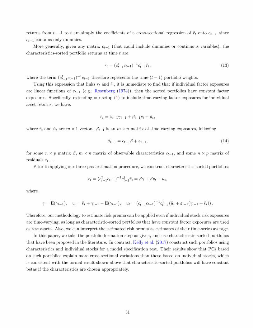
returns from t − 1 to t are simply the coefficients of a cross-sectional regression of rt onto ct−1, since
ct−1 contains only dummies.
More generally, given any matrix ct−1 (that could include dummies or continuous variables), the
characteristics-sorted portfolio returns at time t are:
rt = (cᵀt−1ct−1)−1cᵀt−1rt, (13)
where the term (cᵀt−1ct−1)−1ct−1 therefore represents the time-(t− 1) portfolio weights.
Using this expression that links rt and rt, it is immediate to find that if individual factor exposures
are linear functions of ct−1 (e.g., Rosenberg (1974)), then the sorted portfolios have constant factor
exposures. Specifically, extending our setup (1) to include time-varying factor exposures for individual
asset returns, we have:
rt = βt−1γt−1 + βt−1vt + ut,
where rt and ut are m× 1 vectors, βt−1 is an m× n matrix of time varying exposures, following
βt−1 = ct−1β + εt−1, (14)
for some n × p matrix β, m × n matrix of observable characteristics ct−1, and some n × p matrix of
residuals εt−1.
Prior to applying our three-pass estimation procedure, we construct characteristics-sorted portfolios:
rt = (cᵀt−1ct−1)−1cᵀt−1rt = βγ + βvt + ut,
where
γ = E(γt−1), vt = vt + γt−1 − E(γt−1), ut = (cᵀt−1ct−1)−1cᵀt−1 (ut + εt−1(γt−1 + vt)) .
Therefore, our methodology to estimate risk premia can be applied even if individual stock risk exposures
are time-varying, as long as characteristic-sorted portfolios that have constant factor exposures are used
as test assets. Also, we can interpret the estimated risk premia as estimates of their time-series average.
In this paper, we take the portfolio-formation step as given, and use characteristic-sorted portfolios
that have been proposed in the literature. In contrast, Kelly et al. (2017) construct such portfolios using
characteristics and individual stocks for a model specification test. Their results show that PCs based
on such portfolios explain more cross-sectional variations than those based on individual stocks, which
is consistent with the formal result shown above that characteristic-sorted portfolios will have constant
betas if the characteristics are chosen appropriately.
31

6 Conclusion
We propose a three-pass methodology to estimate the risk premium of observable factors in a linear asset
pricing model, that is consistent even when not all factors in the model are specified and observed. The
methodology relies on a simple invariance result that states that to correct the omitted variable problem
in cases where not all factors are observed, it is sufficient to control for enough factors to span the entire
factor space. In this case, the risk premia for observable factors are consistently estimated even though
the risk exposures cannot be identified. We propose to employ PCA to recover the factor space and
effectively use the PCs as controls in the cross-sectional regressions together with the observable factors.
Our three-pass procedure can be viewed as an extension of both the standard two-pass cross-sectional
regression approach and the mimicking-portfolio estimator of risk premia. In particular, it can be
thought of as a factor-augmented two-pass cross-sectional estimator, where the model adds principal
components of returns as controls in the two-pass regressions, completing the factor space. It can also
be thought as a regularized mimicking-portfolio estimator, in which the factor of interest is projected
onto the PCs of returns (themselves portfolios). As we discuss in the paper, our method represents the
convergence of the two methods, that occurs as n→∞.
Equally important to what we can recover is what we cannot recover if some factors are omitted:
how the pricing kernel loads onto the observed factors, as well as the set of true risk exposures to each
factor. These can only be pinned down under much stronger assumptions – by identifying all the factors
that drive the pricing kernel, and explicitly specifying how they enter the pricing kernel. Instead, a
notable property of factor risk premia is precisely that they can be recovered even without specifying
the identities of all factors, and this is what we focus on in this paper.
The main advantage of our methodology is that it provides a systematic way to tackle the concern
that the model predicted by theory is misspecified because of omitted factors. Rather than relying on
arbitrarily chosen “control” factors or computing risk premia only on subsets of the test assets, our
methodology utilizes the large dimension of testing assets available to span the factor space. It also
explicitly takes into account the possibility of measurement error in any observed factor.
The application of the methodology to workhorse factor models using equity test assets yields sev-
eral compelling results. Contrary to most existing estimates, we find that the risk premium estimate
associated with market risk exposure is positive and significant even when the zero-beta rate is left un-
restricted, and close to the time-series average excess return of the market portfolio. This confirms that
our methodology correctly recovers the risk premium of the market (and similar results hold for other
tradable factors), thus mitigating misspecification concerns. The most interesting results appear for
non-tradable factors. Many standard macroeconomic factors appear insignificant, whereas non-tradable
factors related to various market frictions (like liquidity and intermediary leverage) appear strongly
significant even when considered as part of richer linear pricing models that include additional factors.
Similar results hold when looking across asset classes; the stability of the risk premia estimates for sev-
eral factors across markets suggests the presence of pervasive aggregate risks that can be detected once
factors specific to the various asset classes are properly accounted for – which in this case is achieved
using the three-pass methodology we propose.
32
References
Adrian, T., E. Etula, and T. Muir (2014). Financial intermediaries and the cross-section of asset returns.The Journal of Finance 69 (6), 2557–2596.
Ahn, S. C. and A. R. Horenstein (2013). Eigenvalue ratio test for the number of factors. Econometrica 81,1203–1227.
Ang, A., R. Hodrick, Y. Xing, and X. Zhang (2006). The cross-section of volatility and expected returns.Journal of Finance 61, 259–299.
Asness, C. S., A. Frazzini, and L. H. Pedersen (2013). Quality Minus Junk. Technical report, AQR.
Bai, J. (2003). Inferential Theory for Factor Models of Large Dimensions. Econometrica 71 (1), 135–171.
Bai, J. and Y. Liao (2013). Statistical inferences using large estimated covariances for panel data andfactor models. Technical report, Columbia University.
Bai, J. and S. Ng (2002). Determining the number of factors in approximate factor models. Economet-rica 70, 191–221.
Bai, J. and S. Ng (2006). Evaluating latent and observed factors in macroeconomics and finance. Journalof Econometrics 131 (1), 507–537.
Bai, J. and G. Zhou (2015). Fama–MacBeth two-pass regressions: Improving risk premia estimates.Finance Research Letters 15, 31–40.
Bai, Z. and J. W. Silverstein (2009). Spectral Analysis of Large Dimensional Random Matrices. Springer.
Balduzzi, P. and C. Robotti (2008). Mimicking portfolios, economic risk premia, and tests of multi-betamodels. Journal of Business & Economic Statistics 26, 354–368.
Bernanke, B. S. and K. Kuttner (2005). What explains the stock market’s reaction to federal reservepolicy. The Journal of Finance 60, 1221–1257.
Black, F. (1972). Capital market equilibrium with restricted borrowing. The Journal of Business 45 (3),444–455.
Black, F., M. C. Jensen, and M. Scholes (1972). The Capital Asset Pricing Model: Some EmpiricalTests. In Studies in the Theory of Capital Markets. Praeger.
Breeden, D. T., M. R. Gibbons, and R. H. Litzenberger (1989, June). Empirical Test of theConsumption-Oriented CAPM. The Journal of Finance 44 (2), 231–262.
Bryzgalova, S. (2015). Spurious Factors in Linear Asset Pricing Models. Technical report, StanfordUniversity.
Burnside, C. (2016). Identification and inference in linear stochastic discount factor models with excessreturns. Journal of Financial Econometrics 14 (2), 295–330.
Chamberlain, G. and M. Rothschild (1983). Arbitrage, factor structure, and mean-variance analysis onlarge asset markets. Econometrica 51, 1281–1304.
Cochrane, J. H. (2009). Asset Pricing:(Revised Edition). Princeton university press.
Connor, G., M. Hagmann, and O. Linton (2012). Efficient semiparametric estimation of the fama-frenchmodel and extensions. Econometrica 80 (2), 713–754.
Connor, G. and R. A. Korajczyk (1986). Performance measurement with the arbitrage pricing theory:A new framework for analysis. Journal of Financial Economics 15 (3), 373–394.
33
Connor, G. and R. A. Korajczyk (1988). Risk and return in an equilibrium APT: Application of a newtest methodology. Journal of Financial Economics 21 (2), 255–289.
Fama, E. F. and K. R. French (1993). Common risk factors in the returns on stocks and bonds. Journalof Financial Economics 33 (1), 3–56.
Fama, E. F. and K. R. French (2015). A five-factor asset pricing model. Journal of Financial Eco-nomics 116 (1), 1–22.
Fama, E. F. and J. D. Macbeth (1973). Risk, Return, and Equilibrium: Empirical Tests. Journal ofPolitical Economy 81 (3), 607–636.
Fan, J., Y. Liao, and M. Mincheva (2011). High-dimensional covariance matrix estimation in approxi-mate factor models. Annals of Statistics 39 (6), 3320–3356.
Fan, J., Y. Liao, and M. Mincheva (2013). Large covariance estimation by thresholding principalorthogonal complements. Journal of the Royal Statistical Society, B 75, 603–680.
Fan, J., Y. Liao, and J. Yao (2015). Power enhancement in high-dimensional cross-sectional tests.Econometrica 83 (4), 1497–1541.
Ferson, W. E. and C. R. Harvey (1991). The variation of economic risk premiums. Journal of PoliticalEconomy 99 (2), 385–415.
Frazzini, A. and L. H. Pedersen (2014). Betting against beta. Journal of Financial Economics 111 (1),1–25.
Gagliardini, P., E. Ossola, and O. Scaillet (2016). Time-varying risk premium in large cross-sectionalequity datasets. Econometrica 84 (3), 985–1046.
Gagliardini, P., E. Ossola, and O. Scaillet (2017). A diagnostic criterion for approximate factor structure.Technical report, Swiss Finance Institute.
Gibbons, M., S. A. Ross, and J. Shanken (1989). A test of the efficiency of a given portfolio. Econo-metrica 57 (5), 1121–1152.
Gospodinov, N., R. Kan, and C. Robotti (2013). Chi-squared tests for evaluation and comparison ofasset pricing models. Journal of Econometrics 173 (1), 108–125.
Gospodinov, N., R. Kan, and C. Robotti (2014). Misspecification-Robust Inference in Linear Asset-Pricing Models with Irrelevant Risk Factors. The Review of Financial Studies 27 (7), 2139–2170.
Gospodinov, N., R. Kan, and C. Robotti (2016). Spurious inference in reduced-rank asset-pricingmodels. Technical report, Imperial College London.
Harvey, C. R., Y. Liu, and H. Zhu (2016). ...and the Cross-Section of Expected Returns. The Reviewof Financial Studies 29 (1), 5–68.
He, Z., B. Kelly, and A. Manela (2016). Intermediary asset pricing: New evidence from many assetclasses. Technical report, National Bureau of Economic Research.
Horn, R. A. and C. R. Johnson (2013). Matrix Analysis (Second ed.). Cambridge University Press.
Hou, K. and R. Kimmel (2006). On the estimation of risk premia in linear factor models. Technicalreport, Working Paper, Ohio State University.
Hou, K., C. Xue, and L. Zhang (2015). Digesting anomalies: An investment approach. Review ofFinancial Studies, Forthcoming 28 (3), 650–705.
34

Huberman, G., S. Kandel, and R. F. Stambaugh (1987). Mimicking portfolios and exact arbitragepricing. The Journal of Finance 42 (1), 1–9.
Jagannathan, R. and Z. Wang (1998). An asymptotic theory for estimating beta-pricing models usingcross-sectional regression. The Journal of Finance 53 (4), 1285–1309.
Kan, R. and C. Robotti (2008). Specification tests of asset pricing models using excess returns. Journalof Empirical Finance 15 (5), 816–838.
Kan, R. and C. Robotti (2009). Model comparison using the hansen-jagannathan distance. Review ofFinancial Studies 22 (9), 3449–3490.
Kan, R., C. Robotti, and J. Shanken (2013). Pricing model performance and the two-pass cross-sectionalregression methodology. The Journal of Finance 68 (6), 2617–2649.
Kan, R. and C. Zhang (1999a). GMM tests of stochastic discount factor models with useless factors.Journal of Financial Economics 54 (1), 103–127.
Kan, R. and C. Zhang (1999b). Two-Pass Tests of Asset Pricing Models. The Journal of Finance LIV (1),203–235.
Kelly, B., S. Pruitt, and Y. Su (2017). Characteristics are risk exposures. Technical report, Universityof Chicago.
Kleibergen, F. (2009). Tests of risk premia in linear factor models. Journal of Econometrics 149 (2),149–173.
Kleibergen, F. and Z. Zhan (2014). Mimicking portfolios of macroeconomic factors. Technical report,Brown University Working Paper.
Kleibergen, F. and Z. Zhan (2018). Identification-robust inference on risk premia of mimicking portfoliosof non-traded factors. Journal of Financial Econometrics 16 (2), 155–190.
Kozak, S., S. Nagel, and S. Santosh (2017). Interpreting factor models. Journal of Finance, forthcoming .
Lamont, O. A. (2001, November). Economic tracking portfolios. Journal of Econometrics 105 (1),161–184.
Lehmann, B. N. and D. M. Modest (1988). The empirical foundations of the arbitrage pricing theory.Journal of Financial Economics 21 (2), 213–254.
Lewellen, J., S. Nagel, and J. Shanken (2010). A skeptical appraisal of asset pricing tests. Journal ofFinancial Economics 96 (2), 175–194.
Lucca, D. O. and E. Moench (2015). The pre-FOMC announcement drift. The Journal of Finance 70 (1),329–371.
Ludvigson, S. C. and S. Ng (2009). A factor analysis of bond risk premia. Technical report, NationalBureau of Economic Research.
MacKinlay, A. C. and M. P. Richardson (1991). Using Generalized Method of Moments to Test Mean-Variance Efficiency. The Journal of Finance 46 (2), 511–527.
Malloy, C. J., T. J. Moskowitz, and A. VISSING-JØRGENSEN (2009). Long-run stockholder consump-tion risk and asset returns. The Journal of Finance 64 (6), 2427–2479.
McLean, R. D. and J. Pontiff (2015). Does Academic Research Destroy Stock Return Predictability?The Journal of Finance LXXI (1), 1–48.
35

Moon, H. R. and M. Weidner (2015). Linear regression for panel with unknown number of factors asinteractive fixed effects. Econometrica 83 (4), 1543–1579.
Newey, W. K. and K. D. West (1987). A simple, positive semi-definite, heteroskedasticity and autocor-relation consistent covariance matrix. Econometrica 55, 703–708.
Novy-Marx, R. (2014). Predicting anomaly performance with politics, the weather, global warming,sunspots, and the stars. Journal of Financial Economics 112 (2), 137–146.
Onatski, A. (2010). Determining the number of factors from empirical distribution of eigenvalues.Review of Economics and Statistics 92, 1004–1016.
Onatski, A. (2012). Asymptotics of the principal components estimator of large factor models withweakly influential factors. Journal of Econometrics 168, 244–258.
Pastor, L. and R. F. Stambaugh (2003). Liquidity risk and expected stock returns. Journal of PoliticalEconomy 111 (3), 642–685.
Pesaran, M. and T. Yamagata (2012). Testing CAPM with a large number of assets. Technical report,University of South California.
Roll, R. and S. A. Ross (1980). An empirical investigation of the arbitrage pricing theory. The Journalof Finance 35 (5), 1073–1103.
Rosenberg, B. (1974). Extra-market components of covariance in security returns. Journal of Financialand Quantitative Analysis 9 (2), 263–274.
Ross, S. A. (1976). The Arbitrage Theory of Capital Asset Pricing. Journal of Economics Theory 13,341–360.
Shanken, J. (1992). On the Estimation of Beta Pricing Models. The Review of Financial Studies 5 (1),1–33.
Shanken, J. and G. Zhou (2007). Estimating and testing beta pricing models: Alternative methods andtheir performance in simulations. Journal of Financial Economics 84 (1), 40–86.
Welch, I. (2008). The link between fama-french time-series tests and fama-macbeth cross-sectional tests.Technical report, UCLA.
White, H. (2000). Asymptotic Theory for Econometricians: Revised Edition. Emerald Group PublishingLimited.
36

7 Figures and Tables
Figure 1: First Eight Eigenvalues of the Covariance Matrix of 202 Equity Portfolios
2 4 6 8Eigenvalue
0
0.1
0.2
0.3
0.4
0.5
0.6Eigenvalues 1 to 8
2 4 6 8Eigenvalue
0
0.005
0.01
0.015
0.02
0.025
0.03
0.035Eigenvalues 2 to 8
Note: The left panel reports the first eight eigenvalues of the covariance matrix of our 202 test portfolios. The rightpanel zooms in to the eigenvalues two through eight.
37
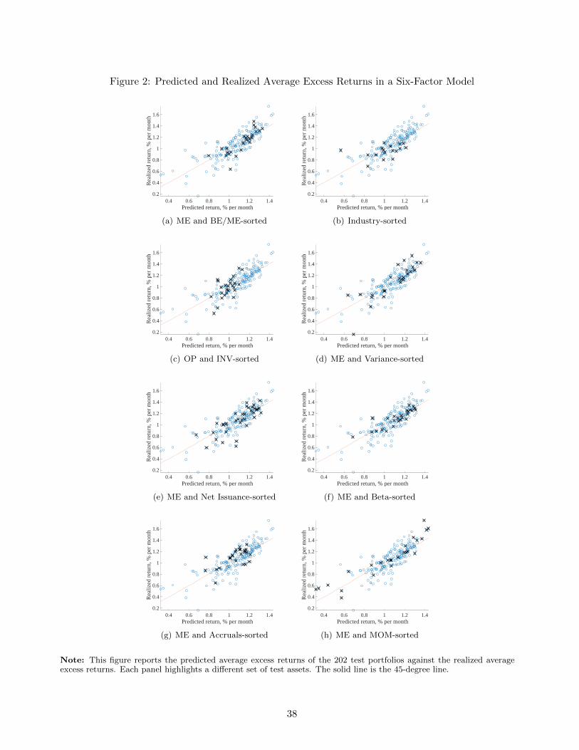
Figure 2: Predicted and Realized Average Excess Returns in a Six-Factor Model
0.4 0.6 0.8 1 1.2 1.4Predicted return, % per month
0.2
0.4
0.6
0.8
1
1.2
1.4
1.6
Rea
lized
ret
urn,
% p
er m
onth
(a) ME and BE/ME-sorted
0.4 0.6 0.8 1 1.2 1.4Predicted return, % per month
0.2
0.4
0.6
0.8
1
1.2
1.4
1.6
Rea
lized
ret
urn,
% p
er m
onth
(b) Industry-sorted
0.4 0.6 0.8 1 1.2 1.4Predicted return, % per month
0.2
0.4
0.6
0.8
1
1.2
1.4
1.6
Rea
lized
ret
urn,
% p
er m
onth
(c) OP and INV-sorted
0.4 0.6 0.8 1 1.2 1.4Predicted return, % per month
0.2
0.4
0.6
0.8
1
1.2
1.4
1.6
Rea
lized
ret
urn,
% p
er m
onth
(d) ME and Variance-sorted
0.4 0.6 0.8 1 1.2 1.4Predicted return, % per month
0.2
0.4
0.6
0.8
1
1.2
1.4
1.6
Rea
lized
ret
urn,
% p
er m
onth
(e) ME and Net Issuance-sorted
0.4 0.6 0.8 1 1.2 1.4Predicted return, % per month
0.2
0.4
0.6
0.8
1
1.2
1.4
1.6
Rea
lized
ret
urn,
% p
er m
onth
(f) ME and Beta-sorted
0.4 0.6 0.8 1 1.2 1.4Predicted return, % per month
0.2
0.4
0.6
0.8
1
1.2
1.4
1.6
Rea
lized
ret
urn,
% p
er m
onth
(g) ME and Accruals-sorted
0.4 0.6 0.8 1 1.2 1.4Predicted return, % per month
0.2
0.4
0.6
0.8
1
1.2
1.4
1.6
Rea
lized
ret
urn,
% p
er m
onth
(h) ME and MOM-sorted
Note: This figure reports the predicted average excess returns of the 202 test portfolios against the realized averageexcess returns. Each panel highlights a different set of test assets. The solid line is the 45-degree line.
38
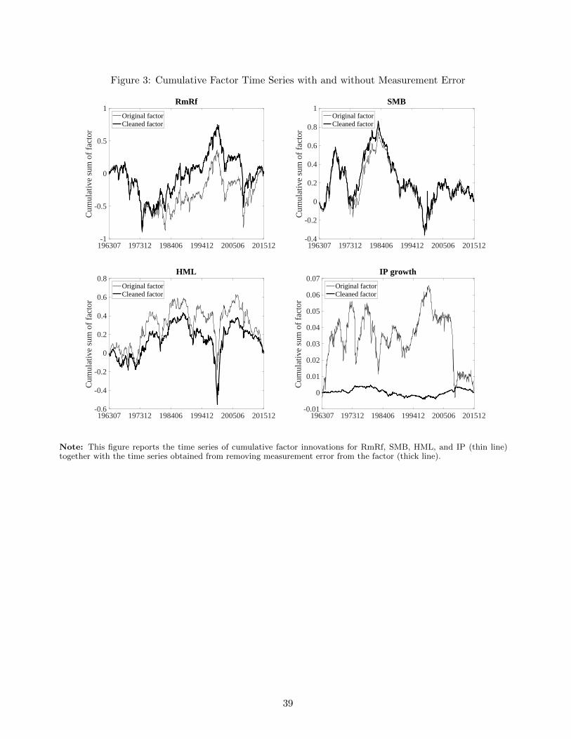
Figure 3: Cumulative Factor Time Series with and without Measurement Error
196307 197312 198406 199412 200506 201512-1
-0.5
0
0.5
1
Cum
ulat
ive
sum
of
fact
or
RmRf
Original factorCleaned factor
196307 197312 198406 199412 200506 201512-0.4
-0.2
0
0.2
0.4
0.6
0.8
1
Cum
ulat
ive
sum
of
fact
or
SMB
Original factorCleaned factor
196307 197312 198406 199412 200506 201512-0.6
-0.4
-0.2
0
0.2
0.4
0.6
0.8
Cum
ulat
ive
sum
of
fact
or
HML
Original factorCleaned factor
196307 197312 198406 199412 200506 201512-0.01
0
0.01
0.02
0.03
0.04
0.05
0.06
0.07
Cum
ulat
ive
sum
of
fact
or
IP growth
Original factorCleaned factor
Note: This figure reports the time series of cumulative factor innovations for RmRf, SMB, HML, and IP (thin line)together with the time series obtained from removing measurement error from the factor (thick line).
39
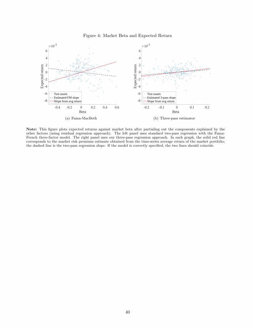
Figure 4: Market Beta and Expected Return
-0.4 -0.2 0 0.2 0.4 0.6Beta
-8
-6
-4
-2
0
2
4
6
Exp
ecte
d re
turn
10-3
Test assetsEstimated FM slopeSlope from avg return
(a) Fama-MacBeth
-0.2 -0.1 0 0.1 0.2Beta
-8
-6
-4
-2
0
2
4
6
Exp
ecte
d re
turn
10-3
Test assetsEstimated 3-pass slopeSlope from avg return
(b) Three-pass estimator
Note: This figure plots expected returns against market beta after partialing out the components explained by theother factors (using residual regression approach). The left panel uses standard two-pass regression with the Fama-French three-factor model. The right panel uses our three-pass regression approach. In each graph, the solid red linecorresponds to the market risk premium estimate obtained from the time-series average return of the market portfolio;the dashed line is the two-pass regression slope. If the model is correctly specified, the two lines should coincide.
40

Figure 5: Robustness to the Set of Test Portfolios: Resampling Exercise
-2 0 2 4 6 8 10
10-3
0
200
400
600
800RmRf
-2 0 2 4 6 8 10
10-3
0
500
1000
1500
2000
2500
3000SMBHML
-2 0 2 4 6 8 10
10-3
0
200
400
600
800
1000
1200MOM
-2 0 2 4 6 8 10
10-3
0
200
400
600
800
1000
1200ip growth
-2 0 2 4 6 8 10
10-3
0
100
200
300
400
500
600
700Liquidity
-2 0 2 4 6 8 10
10-3
0
200
400
600
800
1000
1200Intermediary (He et al.)Intermediary (Adrian et al.)
Note: This figure reports the histograms of risk premia estimated using the three-pass estimator across subsamples ofthe set of 202 test portfolios. We generate 10,000 subsamples by randomly drawing (without replacement) half of theportfolios from the baseline set of 202 portfolios. In each sample we estimate the risk premium of each factor using thethree-pass estimator, setting p = 6. The histogram reports the frequency of the risk premia estimates across samples.All figures report the same range for the risk premia, between -20bp and 100bp per month.
41

Figure 6: Robustness to the Time Period: Resampling Exercise
-2 0 2 4 6 8 10
10-3
0
100
200
300
400
500
600
700RmRf
-2 0 2 4 6 8 10
10-3
0
500
1000
1500
2000SMBHML
-2 0 2 4 6 8 10
10-3
0
100
200
300
400
500
600MOM
-2 0 2 4 6 8 10
10-3
0
200
400
600
800ip growth
-2 0 2 4 6 8 10
10-3
0
100
200
300
400
500
600
700Liquidity
-2 0 2 4 6 8 10
10-3
0
200
400
600
800
1000
1200
1400Intermediary (He et al.)Intermediary (Adrian et al.)
Note: This figure reports the histograms of risk premia estimated using the three-pass estimator across subsamplesof the time period. We generate 10,000 subsamples by randomly drawing (without replacement) half of the availabletime periods (using all of the portfolios available in the selected periods). In each sample we estimate the risk premiumof each factor using the three-pass estimator, setting p = 6. The histogram reports the frequency of the risk premiaestimates across samples. All figures report the same range for the risk premia, between -20bp and 100bp per month.
42

Tab
le1:
Th
ree-
Pas
sR
egre
ssio
n:
Em
pir
ical
Res
ult
sw
ith
Res
tric
ted
Zer
o-b
eta
Rat
e
two-p
ass
regre
ssio
ntw
o-p
ass
regre
ssio
ntw
o-p
ass
regre
ssio
nM
imic
kin
g-p
ort
f.M
imic
kin
g-p
ort
f.M
imic
kin
g-p
ort
f.th
ree-
pass
regre
ssio
n
no
contr
ols
w/R
mw
/F
F3
w/R
mw
/F
F3
w/
all
ass
ets
Fact
ors
Avg.
Ret
.γ
stder
rγ
stder
rγ
stder
rγ
stder
rγ
stder
rγ
stder
r
Mark
et0.5
00.5
9∗∗∗
(0.1
9)
0.5
9∗∗∗
(0.1
9)
0.4
9∗∗∗
(0.1
8)
0.5
0∗∗∗
(0.1
8)
0.5
0∗∗∗
(0.1
8)
0.5
2∗∗∗
(0.1
8)
0.5
1∗∗∗
(0.1
8)
SM
B0.2
30.6
3∗∗∗
(0.2
0)
0.1
6(0.1
3)
0.1
3(0.1
3)
0.1
1∗∗∗
(0.0
4)
0.2
3∗
(0.1
2)
0.2
5∗∗
(0.1
2)
0.2
4∗
(0.1
3)
HM
L0.3
4−
1.0
2∗∗∗
(0.3
7)
0.4
3∗∗∗
(0.1
4)
0.4
6∗∗∗
(0.1
3)
−0.1
0∗∗
(0.0
4)
0.3
4∗∗∗
(0.1
1)
0.3
4∗∗∗
(0.1
1)
0.2
1∗∗
(0.1
1)
MO
M0.7
1−
1.7
8∗∗∗
(0.6
5)
0.6
9∗∗∗
(0.1
8)
0.9
0∗∗∗
(0.1
7)
−0.0
6∗
(0.0
4)
−0.2
0∗∗∗
(0.0
7)
0.7
1∗∗∗
(0.1
7)
0.7
7∗∗∗
(0.1
7)
RM
W0.2
5−
0.1
6(0.1
4)
−0.0
4(0.1
4)
0.3
2∗∗∗
(0.1
0)
−0.0
5∗∗
(0.0
2)
−0.0
9∗∗
(0.0
4)
0.2
9∗∗∗
(0.0
9)
0.1
5∗∗
(0.0
6)
CM
A0.3
0−
0.4
7∗∗∗
(0.1
8)
0.3
8∗∗∗
(0.1
1)
0.4
9∗∗∗
(0.1
0)
−0.0
9∗∗∗
(0.0
3)
0.1
1∗
(0.0
6)
0.2
7∗∗∗
(0.0
8)
0.1
3∗
(0.0
8)
BA
B0.8
4−
0.6
7(0.5
1)
1.1
1∗∗∗
(0.1
9)
1.3
9∗∗∗
(0.1
9)
−0.0
3(0.0
3)
0.1
6∗∗
(0.0
6)
0.6
5∗∗∗
(0.1
4)
0.5
9∗∗∗
(0.1
0)
QM
J0.3
5−
0.4
5∗∗∗
(0.1
5)
−0.0
2(0.1
3)
0.3
7∗∗∗
(0.1
1)
−0.1
4∗∗∗
(0.0
5)
−0.2
6∗∗∗
(0.0
7)
0.2
2∗∗
(0.1
0)
0.0
5(0.0
8)
Liq
uid
ity
2.1
0∗∗∗
(0.6
5)
4.5
4∗∗∗
(1.0
9)
2.1
6∗∗∗
(0.6
4)
0.2
1∗∗
(0.0
8)
0.2
4∗∗
(0.1
0)
0.2
3(0.2
9)
0.3
3∗∗∗
(0.1
1)
Inte
rm.
(He)
0.7
3∗
(0.4
3)
−0.1
8(0.5
7)
0.1
0(0.5
1)
0.5
2∗∗
(0.2
3)
0.7
4∗∗∗
(0.2
4)
0.5
9∗
(0.3
3)
0.5
0∗∗
(0.2
5)
Inte
rm.
(Adri
an)
1.6
7∗∗∗
(0.2
4)
1.6
8∗∗∗
(0.2
4)
1.7
9∗∗∗
(0.2
4)
0.1
2∗∗
(0.0
6)
0.6
5∗∗∗
(0.1
4)
0.9
5∗∗∗
(0.1
9)
0.8
9∗∗∗
(0.1
5)
NY
tem
p.
−450.7
8∗
(252.2
7)
382.2
7∗∗
(162.3
2)
−12.5
6(1
25.4
9)
−5.8
3(6.3
5)
1.5
4(9.5
2)
43.8
4(5
7.4
8)
−5.1
5(1
0.3
4)
Glo
bal
tem
p.
−5.4
7(4.8
0)
−3.5
2(4.9
1)
0.7
2(2.8
3)
−0.0
2(0.1
0)
0.0
0(0.1
5)
−0.0
3(0.9
9)
−0.1
0(0.1
6)
El
Nin
o73.8
6∗∗∗
(16.7
0)
14.2
2(1
0.6
4)
−23.0
1∗∗∗
(7.0
4)
0.4
4(0.3
5)
0.7
0(0.4
8)
−1.8
3(3.1
0)
0.3
2(0.5
8)
Sunsp
ots
170.3
8(7
27.8
5)
2690.5
1∗∗∗
(530.0
6)
2044.6
1∗∗∗
(484.8
9)
−21.7
0(2
0.2
8)
−12.7
9(2
5.1
2)
−210.6
2(1
60.6
9)
16.7
2(2
7.4
4)
IPgro
wth
−1.2
2∗∗∗
(0.3
5)
−0.2
9∗∗∗
(0.0
5)
−0.3
0∗∗∗
(0.0
5)
−0.0
0(0.0
0)
−0.0
0(0.0
0)
−0.0
2(0.0
1)
−0.0
1(0.0
0)
Macr
oP
C1
87.0
9∗∗∗
(21.1
1)
73.8
3∗∗∗
(19.8
6)
19.2
2(1
4.3
5)
0.8
8(0.5
5)
2.1
7∗∗
(1.0
9)
4.5
6(5.2
2)
2.3
3∗
(1.2
3)
Macr
oP
C2
−17.9
6(1
6.9
8)
−15.2
5(1
9.4
9)
−20.8
6∗
(10.7
0)
−0.7
9∗
(0.4
8)
−1.3
1∗
(0.7
7)
3.3
0(3.6
6)
−1.5
7(0.9
9)
Macr
oP
C3
20.2
1(1
4.0
4)
25.8
6∗∗
(10.5
0)
6.6
5(9.5
0)
−0.5
8(0.4
0)
−0.1
3(0.7
6)
−4.2
1(3.4
7)
−0.1
5(1.0
4)
Cons.
gro
wth
0.4
4∗∗∗
(0.1
6)
0.1
0(0.1
0)
0.0
7(0.0
7)
0.0
0(0.0
0)
0.0
1(0.0
1)
0.0
1(0.0
3)
0.0
1(0.0
1)
Sto
ckhold
erco
ns.
7.3
6∗∗∗
(2.4
0)
4.1
1∗∗∗
(1.3
2)
2.5
8∗∗∗
(0.7
2)
0.0
5(0.0
4)
0.0
3(0.0
6)
−0.1
3(0.3
4)
0.1
2∗∗∗
(0.0
5)
Note
:F
or
each
fact
or,
the
table
rep
ort
sth
eri
skpre
mia
esti
mate
susi
ng
diff
eren
tm
ethods,
wit
hth
ere
stri
ctio
nth
at
the
zero
-bet
ara
teis
equal
toth
eobse
rved
T-b
ill
rate
:“A
vg.
Ret
.”,
the
tim
e-se
ries
aver
age
retu
rnof
the
fact
or,
available
when
the
fact
or
istr
adable
;th
ree
ver
sions
of
the
two-p
ass
cross
-sec
tional
regre
ssio
n,
usi
ng
no
contr
ol
fact
ors
inth
em
odel
,usi
ng
the
mark
et,
and
usi
ng
the
Fam
a-F
rench
thre
efa
ctors
,re
spec
tivel
y;
thre
ever
sions
of
the
mim
ickin
g-
port
folio
esti
mato
r,pro
ject
ing
fact
ors
onto
the
mark
etp
ort
folio,
the
Fam
a-F
rench
thre
efa
ctors
,and
onto
all
202
test
ass
ets,
resp
ecti
vel
y;
and
the
thre
e-pass
esti
mato
rw
epro
pose
inth
ispap
er.
43

Tab
le2:
Th
ree-
Pas
sR
egre
ssio
n:
Em
pir
ical
Res
ult
sw
ith
Unre
stri
cted
Zer
o-b
eta
Rat
e
two-p
ass
regre
ssio
ntw
o-p
ass
regre
ssio
ntw
o-p
ass
regre
ssio
nth
ree-
pass
regre
ssio
nth
ree-
pass
regre
ssio
nth
ree-
pass
regre
ssio
np-v
alu
efo
rno
contr
ols
w/Rm
w/
FF
3p
=4
p=
5p
=6
gw
eak
null
Fact
ors
Avg.
Ret
.γ
stder
rγ
stder
rγ
stder
rγ
stder
rR
2 gγ
stder
rR
2 gγ
stder
rR
2 g
Mark
et0.5
0−
0.2
0(0.2
8)
−0.2
0(0.2
8)
−0.5
7∗∗
(0.2
5)
0.3
7∗
(0.2
0)
98.1
80.3
7∗
(0.2
1)
98.9
30.3
5(0.2
2)
99.0
80.0
0
SM
B0.2
30.1
1(0.1
3)
0.1
9(0.1
3)
0.1
7(0.1
3)
0.2
3∗
(0.1
3)
93.9
00.2
3∗
(0.1
3)
94.8
80.2
3∗
(0.1
3)
97.1
90.0
0
HM
L0.3
40.2
3(0.1
6)
0.2
7∗∗
(0.1
3)
0.2
3∗
(0.1
3)
0.2
1∗
(0.1
1)
66.8
60.2
1∗
(0.1
1)
67.9
00.2
0∗
(0.1
1)
75.3
70.0
0
MO
M0.7
10.6
4∗∗∗
(0.1
9)
0.6
4∗∗∗
(0.1
8)
0.8
1∗∗∗
(0.1
7)
0.7
5∗∗∗
(0.1
8)
91.1
80.7
5∗∗∗
(0.1
8)
91.5
20.7
4∗∗∗
(0.1
8)
92.1
90.0
0
RM
W0.2
5−
0.1
3(0.1
4)
−0.0
9(0.1
4)
0.3
0∗∗∗
(0.1
0)
0.1
3∗∗
(0.0
6)
33.9
30.1
3∗∗
(0.0
7)
37.4
20.1
3∗
(0.0
7)
45.8
10.0
0C
MA
0.3
00.2
8∗∗∗
(0.1
0)
0.3
4∗∗∗
(0.1
1)
0.3
7∗∗∗
(0.0
9)
0.1
4∗
(0.0
8)
44.5
80.1
4∗
(0.0
8)
45.6
80.1
3(0.0
8)
55.3
80.0
0
BA
B0.8
40.5
5∗∗
(0.2
4)
1.2
9∗∗∗
(0.2
8)
1.2
7∗∗∗
(0.2
3)
0.5
5∗∗∗
(0.1
1)
45.4
00.5
5∗∗∗
(0.1
1)
45.8
50.5
4∗∗∗
(0.1
2)
49.0
00.0
0
QM
J0.3
50.0
3(0.1
3)
−0.0
2(0.1
3)
0.3
9∗∗∗
(0.1
1)
0.0
7(0.0
8)
59.6
30.0
7(0.0
8)
63.1
30.0
7(0.0
9)
70.4
30.0
0
Liq
uid
ity
0.0
2(0.9
7)
3.5
8∗∗∗
(1.1
7)
0.9
8(0.6
4)
0.2
6∗∗
(0.1
2)
11.9
90.2
6∗∗
(0.1
2)
12.0
20.2
5∗∗
(0.1
2)
12.0
20.0
0
Inte
rm.
(He)
0.0
2(0.6
4)
−0.7
7(0.5
4)
−0.2
2(0.5
1)
0.3
0(0.2
7)
60.1
00.2
9(0.2
9)
62.0
80.2
8(0.3
0)
62.1
30.0
0In
term
.(A
dri
an)
1.2
5∗∗∗
(0.3
2)
1.3
0∗∗∗
(0.3
3)
1.3
2∗∗∗
(0.2
5)
0.7
9∗∗∗
(0.1
6)
49.2
80.7
8∗∗∗
(0.1
7)
49.2
80.7
7∗∗∗
(0.1
7)
51.5
80.0
0
NY
tem
p.
316.1
1(2
09.0
9)
160.1
7(1
56.7
2)
−31.3
8(1
26.1
4)−
1.3
4(1
0.6
1)
0.5
0−
2.1
3(1
1.5
3)
0.5
0−
1.5
3(1
0.5
4)
0.5
10.8
7G
lobal
tem
p.
2.6
5(4.9
2)
3.4
1(4.6
6)
−3.5
5(2.7
5)
−0.0
7(0.1
7)
1.7
4−
0.0
8(0.1
8)
1.8
5−
0.0
4(0.1
8)
1.8
70.0
3E
lN
ino
−6.3
8(9.4
6)
0.2
9(9.7
5)
−1.9
2(5.9
1)
0.0
1(0.5
9)
0.9
70.0
9(0.6
5)
1.0
10.0
1(0.6
0)
1.0
10.6
6Sunsp
ots
1867.7
0∗∗∗
(668.0
6)
1285.3
1∗∗∗
(448.6
3)
1074.2
0∗∗∗
(409.7
4)
25.1
2(2
7.7
4)
0.7
123.1
7(3
0.4
1)
0.7
320.5
4(2
7.3
3)
0.8
70.5
7
IPgro
wth
−0.1
6∗∗∗
(0.0
5)
−0.1
6∗∗∗
(0.0
5)
−0.1
5∗∗∗
(0.0
4)
−0.0
0(0.0
0)
0.3
0−
0.0
0(0.0
0)
0.3
4−
0.0
0(0.0
0)
0.5
20.8
0
Macr
oP
C1
32.6
5∗
(18.3
6)
47.7
1∗∗
(19.8
5)
−21.3
3(1
3.2
0)
2.0
4(1.2
5)
1.4
01.9
9(1.2
5)
1.6
31.9
0(1.2
4)
1.6
40.1
0M
acr
oP
C2
−21.1
4(1
6.2
3)
−37.0
6∗∗
(17.3
8)
20.8
4∗∗
(10.2
3)
−1.2
9(0.9
9)
1.9
8−
1.2
7(1.0
0)
2.0
0−
1.2
1(0.9
9)
2.0
20.0
6M
acr
oP
C3
29.2
5∗∗
(12.4
2)
10.1
1(1
0.7
5)
−13.8
6(9.5
6)
−0.2
3(1.0
6)
1.9
4−
0.2
5(1.0
6)
3.2
9−
0.1
5(1.1
2)
4.4
20.0
0
Cons.
gro
wth
0.1
1(0.1
0)
0.2
8∗∗∗
(0.1
0)
0.1
2∗
(0.0
7)
0.0
1(0.0
1)
3.1
00.0
1(0.0
1)
3.1
20.0
1(0.0
1)
3.6
00.0
0
Sto
ckhold
erco
ns.
0.5
8(1.4
0)
−0.2
3(1.0
9)
0.4
5(0.6
2)
0.0
4(0.0
5)
1.3
30.0
7(0.0
6)
2.6
40.0
6(0.0
6)
2.6
60.2
2
Note
:F
or
each
fact
or,
the
table
rep
ort
sth
eri
skpre
mia
esti
mate
susi
ng
diff
eren
tm
ethods,
wit
hunre
stri
cted
zero
-bet
ara
te(e
stim
ate
dbut
not
rep
ort
edin
the
table
for
reaso
ns
of
space
):“A
vg.
Ret
.”,
the
tim
e-se
ries
aver
age
retu
rnof
the
fact
or,
available
when
the
fact
or
istr
adable
;th
ree
ver
sions
of
the
two-p
ass
cross
-sec
tional
regre
ssio
n,
usi
ng
no
contr
ol
fact
ors
inth
em
odel
,usi
ng
the
mark
et,
and
usi
ng
the
Fam
a-F
rench
thre
efa
ctors
,re
spec
tivel
y;
and
thre
ever
sions
of
the
thre
e-pass
esti
mato
rw
epro
pose
inth
ispap
er,
usi
ng
4,
5,
and
6pri
nci
pal
com
ponen
ts,
resp
ecti
vel
y.T
he
thre
e-pass
resu
lts
rep
ort
,in
addit
ion
toth
ees
tim
ate
of
the
risk
pre
miu
mand
the
standard
erro
r,th
eR
2of
the
tim
e-se
ries
regre
ssio
nof
the
fact
or
onto
the
PC
s.T
he
table
does
not
rep
ort
resu
lts
wit
hth
em
imic
kin
g-p
ort
folio
appro
ach
bec
ause
itdoes
not
allow
for
unre
stri
cted
zero
-bet
ara
te.
The
last
colu
mn
inth
eta
ble
rep
ort
sth
ep-v
alu
eof
aW
ald
test
for
the
null
that
the
obse
rvable
fact
org t
isw
eak,
usi
ngp
=6.
44

Table 3: Loading of Observable Factors onto Latent Factors (% of Variation Explained)
Factors Factor 1 Factor 2 Factor 3 Factor 4 Factor 5 Factor 6
Market 91.0 6.3 1.7 0.1 0.8 0.2
SMB 31.0 64.0 0.6 0.9 1.0 2.4
HML 7.0 1.3 75.5 4.9 1.4 9.9
MOM 3.1 0.3 2.0 93.5 0.4 0.7
RMW 17.2 37.4 15.4 4.1 7.6 18.3CMA 19.8 0.0 60.6 0.1 2.0 17.5
BAB 0.9 3.6 72.7 15.4 0.9 6.4
QMJ 57.3 15.9 2.4 9.0 5.0 10.4
Liquidity 95.0 2.8 1.8 0.2 0.2 0.0
Interm. (He et al) 81.2 12.5 0.1 2.9 3.2 0.1Interm. (Adrian et al) 20.3 6.8 52.0 16.4 0.0 4.5
NY temp. 21.7 8.6 46.5 19.7 1.1 2.4Global temp. 0.5 85.9 5.8 0.9 5.4 1.4El Nino 58.8 2.0 9.0 25.8 4.1 0.3Sunspots 41.9 2.4 2.4 34.8 2.5 16.0
IP growth 11.9 3.5 2.3 39.4 8.2 34.7
Macro PC 1 58.0 2.9 24.4 0.0 13.9 0.8Macro PC 2 81.9 13.0 2.3 0.6 1.0 1.2Macro PC 3 23.7 1.0 16.3 3.0 30.4 25.6
Cons. growth 26.5 54.4 5.0 0.1 0.5 13.5
Stockholder cons. 17.9 23.2 2.6 6.5 49.2 0.6
Note: The table reports the decomposition of the variance of the observable factors gt explained by the six latentfactors. Each row adds up to 100%.
45

Table 4: Risk Premia across Asset Classes
202 equity FF25 + 100 non-equity 100 non-equity
Factors Avg ret γ stderr R2g γ stderr R2
g γ stderr R2g
Market 0.47 0.26 (0.24) 98.85 0.73∗∗∗ (0.23) 89.84 0.68∗∗∗ (0.22) 52.37
SMB 0.18 0.17 (0.14) 94.71 0.22∗ (0.12) 31.13 0.15∗∗ (0.06) 2.08
HML 0.41 0.25∗ (0.13) 74.33 0.16∗∗ (0.07) 10.43 0.07 (0.07) 4.44
MOM 0.67 0.59∗∗∗ (0.20) 79.32 −0.30 (0.18) 6.49 −0.27 (0.18) 6.55
RMW 0.29 0.15∗ (0.08) 48.06 −0.17∗∗∗ (0.05) 11.27 −0.16∗∗∗ (0.05) 7.10
CMA 0.40 0.17∗ (0.09) 49.03 −0.04 (0.06) 14.17 −0.10 (0.06) 9.35
BAB 0.87 0.55∗∗∗ (0.12) 43.90 0.22∗∗ (0.09) 7.05 0.16 (0.12) 9.68
QMJ 0.38 0.09 (0.10) 68.82 −0.44∗∗∗ (0.11) 45.15 −0.41∗∗∗ (0.11) 26.95
Liquidity 0.21 (0.13) 11.76 0.24 (0.18) 11.45 0.21 (0.18) 5.88
Interm. (He et al) 0.25 (0.28) 62.21 1.03∗∗∗ (0.30) 52.14 0.94∗∗∗ (0.31) 34.95
Interm. (Adrian et al) 0.69∗∗∗ (0.16) 46.42 0.50∗∗∗ (0.11) 14.91 0.35∗∗∗ (0.09) 6.93
NY temp. 0.11 (10.81) 0.63 6.84 (22.41) 1.26 −2.39 (23.40) 1.91
Global temp. −0.04 (0.17) 1.92 −0.18 (0.37) 0.58 −0.19 (0.42) 0.59
El Nino 0.02 (0.64) 1.48 1.75 (1.18) 1.14 1.79 (1.21) 0.95
Sunspots 26.37 (29.80) 0.90 −10.38 (46.08) 0.86 −6.54 (48.91) 0.88
IP growth −0.00 (0.00) 0.79 0.00 (0.01) 0.96 −0.01 (0.01) 3.43
Macro PC 1 1.66 (1.27) 1.57 0.02 (2.82) 2.24 0.84 (2.69) 1.92
Macro PC 2 −0.81 (0.90) 1.49 −1.95 (1.69) 2.64 −1.70 (1.79) 2.32
Macro PC 3 −0.55 (1.14) 4.96 −3.80∗∗ (1.55) 7.36 −3.68∗∗ (1.87) 7.09
Cons. growth 0.00 (0.01) 3.30 0.03 (0.03) 3.69 0.04∗ (0.03) 2.31
Stockholder cons. 0.05 (0.06) 2.46 0.12 (0.20) 2.50 0.13 (0.23) 3.11
Note: The table reports the results of risk premia estimation for various models using our three-pass procedure. Theleft side of the panel uses 202 equity portfolios as test assets. The center panel uses the 25 Fama-French portfoliosplus 100 non-equity assets. The right panel uses only the 100 non-equity assets. Sample period covers 1970-2012. Thenumber of factors p used is 5 for the left and middle panel and 6 for the right panel.
46

Table 5: Alternative Objective Function for Latent Factor Estimation
PCA (w = 0) CK (w = 1)
Factors p = 4 p = 5 p = 6 p = 4 p = 5 p = 6
Market 0.51 0.52 0.52 0.51 0.52 0.52
SMB 0.24 0.23 0.23 0.24 0.24 0.23
HML 0.21 0.21 0.22 0.22 0.22 0.22
MOM 0.77 0.76 0.76 0.81 0.80 0.81
RMW 0.15 0.15 0.15 0.15 0.16 0.15
CMA 0.13 0.13 0.13 0.14 0.14 0.14
BAB 0.59 0.60 0.60 0.61 0.62 0.62
QMJ 0.05 0.06 0.05 0.06 0.07 0.06
Liquidity 0.33 0.33 0.33 0.34 0.34 0.34
Interm. (He et al) 0.50 0.51 0.51 0.49 0.51 0.51
Interm. (Adrian et al) 0.89 0.89 0.90 0.92 0.92 0.93
NY temp. -5.15 -5.66 -5.70 -5.07 -5.53 -5.58
Global temp. -0.10 -0.05 -0.05 -0.09 -0.05 -0.05
El Nino 0.32 0.39 0.39 0.31 0.38 0.38
Sunspots 16.72 13.74 13.29 18.31 15.16 14.72
IP growth -0.01 -0.01 -0.01 -0.01 -0.01 -0.01
Macro PC 1 2.33 2.38 2.38 2.37 2.42 2.42
Macro PC 2 -1.57 -1.58 -1.58 -1.59 -1.60 -1.60
Macro PC 3 -0.15 -0.07 -0.06 -0.13 -0.05 -0.05
Cons. growth 0.01 0.01 0.01 0.01 0.01 0.01
Stockholder cons. 0.12 0.17 0.17 0.13 0.18 0.18
Note: The table reports the results of risk premia estimation for various models using our three-pass procedure, usingdifferent penalty functions to extract the latent factors. We report results for p = 4, 5, 6. The left panel uses standardPCA as in our baseline case. The right panel extracts factors using the Connor and Korajczyk (1986, 1988) approach,which gives weight to the cross-sectional R2. Following Connor and Korajczyk (1986, 1988), the zero-beta rate is imposedto be equal to the risk-free rate. Sample period covers 1970-2012.
47

Appendix
A Assumptions and Technical Details
We need more notation. We use λj(A), λmin(A), and λmax(A) to denote the jth, the minimum, and
the maximum eigenvalues of a matrix A. By convention, λ1(A) = λmax(A). In addition, we use ‖A‖1,
‖A‖∞, ‖A‖, and ‖A‖F to denote the L1 norm, the L∞ norm, the operator norm (or L2 norm), and
the Frobenius norm of a matrix A = (aij), that is, maxj∑
i |aij |, maxi∑
j |aij |,√λmax(AᵀA), and√
Tr(AᵀA), respectively. We also use ‖A‖MAX = maxi,j |aij | to denote the L∞ norm of A on the vector
space.
Let (P,Ω,F) be the probability space. K is a generic constant that may change from line to line.
We say a sequence of centered multivariate random variables ytt≥1 satisfy the exponential-type tail
condition, if there exist some constants a and b, such that P (|yit| > y) ≤ exp−(y/b)a, for all i and
t. We say a sequence of random variables satisfy the strong mixing condition if the mixing coefficients
satisfy αm ≤ exp(−Kmc), for m = 1, 2, . . ., and some constants c > 0 and K > 0.
For clarity, we restate the assumptions on the dynamics of returns and factors, i.e., (1) and (2),
introduced in the main text:
Assumption A.1. Suppose that ft is a p × 1 vector of asset pricing factors, and that rt denotes an
n× 1 vector of excess returns of the testing assets. The pricing model satisfies:
rt = βγ + βvt + ut, ft = µ+ vt, E(vt) = E(ut) = 0, and Cov(ut, vt) = 0,
where vt is a p× 1 vector of innovations of ft, ut is a n× 1 vector of idiosyncratic components, β is an
n× p factor loading matrix, and γ is the p× 1 risk premia vector.
Assumption A.2. There is an observable d× 1 vector, gt, of factor proxies, which satisfies:
gt = ξ + ηvt + zt, E(zt) = 0, and Cov(zt, vt) = 0,
where η, the loading of g on v, is a d×p matrix, ξ is a d×1 constant, and zt is a d×1 measurement-error
vector.
Next, we impose some restrictive assumptions, which are only used in Proposition 1 and Section
3.4 to illustrate the intuition of our result and the connection between the two-pass cross-sectionals
regression and the factor mimicking portfolios. Our asymptotic analysis below does not rely on this
assumption.
Assumption A.3. Suppose that vt, zt, and ut in (1) are stationary time series independent of β,
respectively, and that the weights of the spanning portfolios, rt, are given by the n × p matrix w with
p ≥ p. The covariance matrices of vt and ut, i.e., Σv and Σu, and the loading of zt on ut := wᵀrt, i.e.,
βz,u, satisfy the following conditions: λ−1min(Σv) = Op(1),
∥∥∥βz,uβ∥∥∥MAX
= Op(1), λ−1min(βᵀβ) = Op(1),
λmax(Σu) = Op(snn−1), where β := wᵀβ, sn = op(n).
48
The condition on λmin(Σv) requires the set of factors in (1) to have a full rank covariance matrix;
the second condition on βz,uβ restricts the exposure of gt to the idiosyncratic errors ut; the condition
on βᵀβ resembles the usual pervasiveness assumption that guarantees nontrivial exposure of spanning
portfolios to factors; the last restriction on Σu ensures that the idiosyncratic errors are diversifiable.
These conditions turn out sufficient for the difference between the risk premium of gt and that of its
factor-mimicking portfolios to diminish as shown in Proposition 1.
There are two notable choices of w that are relevant for our study. The first case sets w = n−1/2In,
that is, gt is projected onto the entire set of test assets rt. In this case, the conditions in Assumption
A.3 are similar to the identification conditions of the approximate factor models. In particular, the
last condition is more general than the bounded eigenvalue assumption introduced in Chamberlain and
Rothschild (1983). The second choice sets w = n−1βH, for any invertible matrix H. That is, the base
portfolios are constructed using weights proportional to the exposure of the test assets. Because β is
unknown, this case is not feasible. However, it is precisely what motivates the (feasible) construction
of the three-pass estimator: w = β(βᵀβ)−1.
The following assumptions are more general, which we rely on to derive the asymptotic results in
the paper. These high-level assumptions can be justified using stronger and more primitive conditions
such as those in Assumption A.3.
We proceed with the idiosyncratic component ut, and define, for any t, t′ ≤ T :
γn,tt′ = E
(n−1
n∑i=1
uituit′
).
Assumption A.4. There exists a positive constant K, such that for all n and T ,
(i) T−1T∑t=1
T∑t′=1
|γn,tt′ | ≤ K, max1≤t≤T
γn,tt ≤ K.
(ii) T−2T∑s=1
T∑t=1
E
n∑j=1
(ujsujt − E(ujsujt))
2
≤ Kn.
Assumption A.4 is similar to part of Assumption C in Bai (2003), which imposes restrictions on the
cross-sectional dependence and heteroskedasticity of ut.
Assumption A.5. The factor innovation V satisfies:
‖v‖MAX = Op(T−1/2),
∥∥T−1V V ᵀ − Σv∥∥
MAX= Op(T
−1/2),
where Σv is a p× p positive-definite matrix and 0 < K1 < λmin(Σv) ≤ λmax(Σv) < K2 <∞.
Assumption A.5 imposes rather weak conditions on the time series behavior of the factors. It
certainly holds if factors are stationary and satisfy the exponential-type tail condition and the strong
mixing condition, see, Fan et al. (2013).
49

Assumption A.6. The factor loadings matrix β satisfies∥∥∥n−1βᵀβ − Σβ∥∥∥ = op(1), as n→∞,
where Σβ is a p× p positive-definite matrix and 0 < K1 < λmin(Σβ) ≤ λmax(Σβ) < K2 <∞.
This is the key identifying assumption that imposes all factors to be pervasive and hence excludes
weaker ones. Onatski (2012) develops the inference methodology in a framework that allows for weak
factors using a Pitman-drift-like asymptotic device.
Assumption A.7. The factor loadings matrix β and the idiosyncratic error ut satisfy the following
moment conditions, for all 1 ≤ j ≤ p and for all n and T :
(i) E
T∑t=1
(n∑i=1
βijuit
)2
≤ KnT.
(ii) E
(T∑t=1
n∑i=1
βijuit
)2
≤ KnT.
This assumption can be shown from the stronger cross-sectional independence assumption between
β and ut as well as some moment conditions on β, which are imposed by Bai (2003).
Assumption A.8. The residual innovation Z satisfies:
‖z‖MAX = Op(T−1/2),
∥∥T−1ZZᵀ − Σz∥∥
MAX= Op(T
−1/2),
where Σz is positive-definite and 0 < K1 < λmin(Σz) ≤ λmax(Σz) < K2 <∞. In addition,
‖ZV ᵀ‖MAX = Op(T1/2).
Similar to Assumption A.5, Assumption A.8 holds if zt is stationary, and satisfies the exponential-
type tail condition and some strong mixing condition. It is more general than the i.i.d. assumption on
zt, which also applies to non-tradable factor proxies in the empirical applications.
Assumption A.9. For all n and T , and i, j ≤ p, l ≤ d, the following moment conditions hold:
(i) E
n∑k=1
(T∑t=1
vjtukt
)2
≤ KnT.
(ii) E
(T∑t=1
n∑k=1
vituktβkj
)2
≤ KnT.
Assumption A.9 resembles Assumption D in Bai (2003). The variables in each summation have zero
means, so that the required rate can be justified under more primitive assumptions. In fact, it holds
trivially if vt and ut are independent.
50
Assumption A.10. For all n and T , and l ≤ d, j ≤ p, the following moment conditions hold:
(i) E
n∑k=1
(T∑t=1
zltukt
)2
≤ KnT.
(ii) E
(T∑t=1
n∑k=1
zltuktβkj
)2
≤ KnT.
Similar to Assumption A.9, Assumption A.10 restricts the dependence between the idiosyncratic
component ut and the projection residual zt. If zt, ut, and β are independent, (i) - (ii) are easy to
verify. For a tradable portfolio factor in gt, we can interpret its corresponding zt as certain undiversified
idiosyncratic risk, since zt is a portfolio of ut as implied from Assumptions A.1 and A.2. It is thereby
reasonable to allow for dependence between zt and ut. For non-tradable factors, zts can also be correlated
with ut in general.
Assumption A.11. As T →∞, the following joint central limit theorem holds:
T 1/2
(T−1vec(ZV ᵀ)
v
)L−→ N
((0
0
),
(Π11 Π12
Πᵀ12 Π22
)),
where Π11, Π12, and Π22 are dp× dp, dp× p, and p× p matrices, respectively, defined as:
Π11 = limT→∞
1
TE (vec(ZV ᵀ)vec(ZV ᵀ)ᵀ) ,
Π12 = limT→∞
1
TE(vec(ZV ᵀ)ιᵀTV
ᵀ) ,Π22 = lim
T→∞
1
TE(V ιT ι
ᵀTV
ᵀ) .Assumption A.11 describes the joint asymptotic distribution of ZV ᵀ and V ιT . Because the dimen-
sions of these random processes are finite, this assumption is a fairly standard result of some central
limit theorem for mixing processes, (e.g., Theorem 5.20 of White (2000)). Needless to say, it is stronger
than Assumption A.5, which is sufficient for identification and consistency.
Assumption A.12 restates the assumptions on the dynamics of (12) in the main text.
Assumption A.12. Suppose the cross-section of asset returns rt follows
rt = α+ ιnγ0 + βγ + βvt + ut,
where the cross-sectional pricing error α is i.i.d., independent of β, u and v, with mean 0, standard
deviation σα > 0, and a finite fourth moment.
Assumption A.13. There exists a p× 1 vector β0, such that∥∥n−1βᵀιn − β0
∥∥MAX
= op(1). Moreover,
the matrix (1 βᵀ0β0 Σβ
)is of full rank.
51
This assumption is imposed only in the case when we allow for and estimate the zero-beta rate. The
rank condition ensures that in the limit the factor loadings and ιn are not perfectly correlated in the
cross section, and in particular, that the zero-beta rate γ0 is identifiable.
Assumption A.14. Define, for any i, i′ ≤ n, t, t′ ≤ T ,
E(uitui′t) = σii′,t, and E(uitui′t′) = σii′,tt′ .
The following moment conditions hold, for all n and T , and i, j ≤ p, l ≤ d,
(i) max1≤t≤T
|σii′,t| ≤ |σii′ |, for some σii′ . In addition, n−1n∑i=1
n∑i′=1
|σii′ | ≤ K.
(ii) n−1T−1n∑i=1
n∑i′=1
T∑t=1
T∑t′=1
|σii′,tt′ | ≤ K.
(iii) E
(T∑t=1
n∑k=1
vjtukt
)2
≤ KnT.
Assumption A.14 imposes restrictions on the time series dependence of ut. Stationarity of ut is
not required. Eigenvalues of the residual covariance matrices E(utuᵀt ) are not necessarily bounded.
Assumption A.14 is similar to part of Assumption C in Bai (2003). We only need it when we allow for
a zero-beta rate.
Assumption A.15. The following conditions hold:
(i)T∑t′=1
|γn,tt′ | ≤ K, for all t.
(ii)n∑
i′=1
|σii′ | ≤ K, for all i.
This assumption is identical to Assumption E in Bai (2003). It restricts the eigenvalues of E(utuᵀt )
and E(uᵀtut) to be bounded as the dimension increases, because the L∞-norm is stronger than the
operator norm for symmetric matrices. We need this to bound the estimation error of factors uniformly
over t, which in turn leads to the consistency of the asymptotic variance estimation.
For the same reason, we also need Assumption A.16, which Fan et al. (2011) and Fan et al. (2015)
also adopt:
Assumption A.16. The sequence of ut, vt, ztt≥1 is jointly strong mixing, and satisfies the exponential-
type tail condition. Moreover, for all t′, t ≤ T ,
E (uᵀtut′ − Euᵀtut′)4 ≤ Kn2, E ‖βᵀut‖4 ≤ Kn2.
52

B Additional Results
B.1 Mimicking Portfolios
Proposition 1. Suppose Assumptions A.1 - A.3 hold. The risk premium of the mimicking portfolio
that is maximally correlated with gt, γMPg , satisfies: γMP
g − ηγ = op(1), as n→∞.
B.2 Limiting Distribution of the Denoised Factors
As discussed above, our framework allows for measurement error in the observable factor proxies g.
Theorem 4 in the main text indicates that we can separate the error from the factors using the extracted
PCs. Moreover, we can conduct inference on gt, provided an additional assumption:
Assumption B.17. For each t, as n→∞,
n−1/2βᵀutL−→ N (0,Ωt) ,
where, writing β = (β1 : β2 : . . . : βn)ᵀ,
Ωt = limn→∞
1
n
n∑i=1
n∑i′=1
βiβᵀi′E(uitui′t). (B.1)
Assumption B.17 is identical to Assumption F3 in Bai (2003), which is used to describe the asymp-
totic distribution of the estimated factors at each point in time.
Theorem 8. Under Assumptions A.2, and A.4 –A.12, A.15, A.16, and B.17, and suppose that pp−→ p,
then as n, T →∞, we have
Ψ−1/2t (gt − ηvt)
L−→N (0, Id),
where Ψt = T−1Ψ1t + n−1Ψ2t,
Ψ1t =(
vᵀt (Σv)−1 ⊗ Id)
Π11
((Σv)−1 vt ⊗ Id
)−(vᵀt (Σv)−1 ⊗ Id
)Π12η
ᵀ
− ηΠᵀ12
((Σv)−1 vt ⊗ Id
)+ ηΠ22η
ᵀ, and
Ψ2t =η(
Σβ)−1
Ωt
(Σβ)−1
ηᵀ.
In Bai (2003), the latent factors can be estimated at the n−1/2-rate, provided that n1/2T−1 → 0. In
our setting, the estimation error consists of the errors in estimating η and vt. Because η is estimated
up to a T−1/2-rate error which dominates T−1 terms, the convergence rate of gt does not rely on any
relationship between n and T .
53

B.3 Asymptotic Covariance Matrix
To estimate the asymptotic covariance matrices Ψ1t and Ψ2t in Theorem 8, we can simply replace vt,
Σv, Π11, Π12, Π22, η, Σβ by their sample analogues, vt, Σv, Π11, Π12, Π22, η, Σβ, in the Ψ1t and Ψ2t
constructions. With respect to Ωt, we need an additional assumption:
Assumption B.18. The innovation uit is stationary, and its covariance matrix Σu is sparse, i.e., there
exists some h ∈ [0, 1/2), with ωT = (log n)1/2T−1/2 + n−1/2, such that
sn = max1≤i≤n
n∑i′=1
|Σuii′ |h, where sn = op
((ω1−hT + n−1 + T−1
)−1).
Given this assumption, (B.1) and its estimator can be rewritten as
Ω = limn→∞
1
nβᵀΣuβ, and Ωt = Ω =
1
nβᵀΣuβ, (B.2)
where, for 1 ≤ i, i′ ≤ n,
Σuii′ =
Σuii, i = i′
sii′(Σuii′), i 6= i′
, Σu =1
T
T∑t=1
utuᵀt ,
and sii′(z) : R→ R is a general thresholding function with an entry dependent threshold τii′ such that
(i) sii′(z) = 0 if |z| < τii′ ; (ii) |sii′(z) − z| ≤ τii′ ; and (iii) |sii′(z) − z| ≤ aτ2ii′ , if |z| > bτii′ , with some
a > 0 and b > 1. τii′ can be chosen as:
τii′ = c(ΣiiΣi′i′)1/2ωT , for some constant c > 0.
Bai and Liao (2013) adopt a similar estimator of Σu for efficient estimation of factor models.
With estimators of their components constructed, our estimators for Ψ1t and Ψ2t are defined as:
Ψ1t =T−1(
vᵀt (Σv)−1 ⊗ Id)
Π11
((Σv)−1vt ⊗ Id
)−(vᵀt (Σv)−1 ⊗ Id
)Π12η
ᵀ − ηΠᵀ12
((Σv)−1vt ⊗ Id
)+ ηΠ22η
ᵀ,
Ψ2t =n−1η(
Σβ)−1
Ωt
(Σβ)−1
ηᵀ,
where Ωt is given by (B.2). The next theorem establishes the desired consistency of Ψ1t and Ψ2t:
Theorem 9. Under Assumptions A.2, A.3 – A.16, B.17, B.18, we have
Ψ1t −Ψ1tp−→ 0, and Ψ2t −Ψ2t
p−→ 0.
54

C Simulations
In this section, we study the finite sample performance of our inference procedure using Monte Carlo
simulations. We consider a five-factor data-generating process, where the latent factors are calibrated to
match the de-noised five Fama-French factors (RmRf, SMB, HML, RMW, CMA, see Fama and French
(2015)) from our empirical study. Suppose that we do not observe all five factors, but instead some
noisy version of the three Fama-French factors (RmRf, SMB, HML, see Fama and French (1993)), plus a
potentially spurious macro factor calibrated to industrial production growth (IP) in our empirical study.
Our simulations, therefore, include both the issue of omitted factors and that of a spurious factor. We
calibrate the parameters γ0, γ, η, Σv, Σz, Σu, (σα)2, β0, and Σβ to exactly match their counterparts in
the data (in our estimation of the Fama-French five-factor model). We then generate the realizations
of vt, zt, ut, α, and β from a multivariate normal using the calibrated means and covariances.
We report in Tables C1, C2, and C3 the bias and the root-mean-square error of the estimates using
standard two-pass regressions and our three-pass approach. We choose different numbers of factors to
estimate the model, p = 4, 5, and 6, whereas the true value is 5. The five rows in each panel provide
the results for the zero-beta rate, RmRf, SMB, HML, and IP, respectively. Throughout these tables,
we find that the three-pass estimators with p = 5 or 6 outperform the other estimators, in particular
when n and T are large. By comparison, the two-pass estimates have substantial biases. Moreover, the
biases for the market factor premium are substantial and negative even when n and T are large. The
three-pass estimator with p = 4 has an obvious bias, compared to the cases with p = 5 and 6, because
an omitted-factor problem still affects it (4 factors do not span the entire factor space).
We then plot in Figure C1 the histograms of the standardized risk premia estimates using Fama-
MacBeth standard errors for the two-pass estimator (right column) and the estimated asymptotic stan-
dard errors for the three-pass method with p = 5 (left column).19 The histograms on the right deviate
substantially from the standard normal distribution, whereas those on the left match the normal dis-
tribution very well, which verifies our central limit results despite a small sample size T = 240 and a
moderate dimension n = 200. There exist some small higher order biases for γ0, which would disappear
with a larger n and T in simulations not included here.
Next, we report in Table C4 the estimated number of factors. We choose φ(n, T ) = K(log n +
log T )(n−1/2 + T−1/2), where K = 0.5× λ, λ is the median of the first pmax eigenvalues of n−1T−1RᵀR.
The median eigenvalue helps adjust the magnitude of the penalty function for better finite sample
accuracy. Although the estimator is consistent, it cannot give the true number of factors without error,
in particular when n or T is small, potentially due to the ad-hoc choice of tuning parameters.20 In the
empirical study, we apply this estimator of p and select slightly more factors to ensure the robustness
of the estimates, as suggested by Theorem 5.
Then we evaluate the size and power properties of the proposed test in Section 4.7. To check the size
19We have also implemented the standard errors of the two-pass estimators using the formula given by Bai and Zhou(2015), which provides desirable performance when both n and T are large. However, we do not find substantial differencescompared to the Fama-MacBeth method, so we omit those histograms.
20The eigenvalue ratio-based test by Ahn and Horenstein (2013) does not work well in our simulation setting becausethe first eigenvalue dominates the rest by a wide margin, so that their test often suggests 1 factor.
55

control, we create a purely noisy factor with η = 0 and variance calibrated to be the average variance
of the four factors we consider. The top panel of Table C5 reports the rejection probabilities of the test
statistic under the null. In spite of slight over-rejection, the size control is acceptable given the moderate
sizes of n and T . To evaluate the power, we report on the lower panel the average rejection probabilities
when the null is false (η 6= 0). We test for factors with a variety of the signal-to-noise strength measured
by R2g. These factors only load on the market factor, and share the same total variance calibrated to
be the average variance as above, with R2gs being 2.5%, 5%, and 10%, respectively. As expected, we
observe the rejection probability elevates to 100% as R2g increases.
Finally, we compare the performance of these estimators with the mimicking portfolio estimators
under more restrictive dynamics in which γ0 is known and α = 0. So we estimate the model using (8)
and excess returns. We consider two sets of mimicking portfolios: one set (MP3) uses three portfolios
as spanning assets to project factors, where portfolio weights are exactly proportional to the market,
SMB, and HML beta. Using three base assets clearly leads to an omitted variable problem because
these three assets cannot span the space of five factors. The second set of mimicking portfolios (MP)
uses all assets as basis assets for projection. There is no omitted variable bias in this case as we prove
in Proposition 1, but these estimators are not as efficient as the three-pass estimators. They become
infeasible when n > T . Figure C2 verifies these statements. Indeed, the deviation from normality is
clearly visible for all estimators but ours. MP3 and two-pass estimates show visible biases whereas MP
estimates display distortion due to the curse of dimensionality (n is of a similar scale to T ). Tables C6 -
C8 further illustrate that the RMSEs of the mimicking portfolio estimators are often larger than those
of the three-pass estimators, due to large biases of MP3 and large variances of MP.
Overall, the three-pass estimator outperforms the two-pass and mimicking portfolio estimators by
a large margin in almost all cases. The MP estimator using all assets ranks the second, despite being
infeasible when n is greater than T . The biases in the two-pass and MP3 are substantial, yet they are
unfortunately the most common choices in the empirical literature.
56

Table C1: Simulation Results for n = 50
Two-Pass Estimator Three-Pass Estimatorsp = 4 p = 5 p = 6
T Param True Bias RMSE Bias RMSE Bias RMSE Bias RMSE
γ0 0.546 0.252 0.339 0.028 0.210 0.019 0.206 0.042 0.206RmRf 0.372 -0.230 0.514 0.020 0.425 0.019 0.425 -0.016 0.425
120 SMB 0.229 -0.037 0.305 -0.024 0.275 -0.020 0.276 -0.012 0.276HML 0.209 0.010 0.349 -0.111 0.227 -0.088 0.221 -0.071 0.217IP -0.003 -0.015 0.116 0.000 0.009 0.000 0.010 0.000 0.010
γ0 0.546 0.265 0.324 0.085 0.191 0.060 0.177 0.048 0.173RmRf 0.372 -0.214 0.396 -0.033 0.319 -0.029 0.318 -0.020 0.317
240 SMB 0.229 -0.129 0.250 -0.052 0.199 -0.037 0.196 -0.035 0.196HML 0.209 0.082 0.278 -0.074 0.168 -0.049 0.159 -0.043 0.158IP -0.003 -0.024 0.136 0.001 0.006 0.001 0.006 0.001 0.007
γ0 0.546 0.348 0.380 0.051 0.173 0.008 0.146 -0.001 0.145RmRf 0.372 -0.333 0.415 -0.047 0.252 -0.006 0.237 0.003 0.237
480 SMB 0.229 -0.165 0.231 -0.067 0.158 -0.038 0.146 -0.036 0.146HML 0.209 0.211 0.296 -0.008 0.115 -0.022 0.115 -0.020 0.116IP -0.003 -0.040 0.159 0.001 0.004 0.000 0.005 0.000 0.005
Note: In this table, we report the bias (Column “Bias”) and the root-mean-square error (Column “RMSE”) of thezero-beta rate and risk premia estimates using two-pass and three-pass estimators with p = 4, 5, and 6, for n = 50,and T = 120, 240, and 480, respectively. The true data-generating process has five factors, and the parameters arecalibrated based on the de-noised five Fama-French factors (RmRf, SMB, HML, RMW, and CMA). The true zero-betarate is 0.546, and the true risk premia of four noisy yet observed factors (RmRf, SMB, HML, and IP) are provided inthe “True” column. All numbers are in percentages.
Table C2: Simulation Results for n = 100
Two-Pass Estimator Three-Pass Estimatorsp = 4 p = 5 p = 6
T Param True Bias RMSE Bias RMSE Bias RMSE Bias RMSE
γ0 0.546 0.434 0.482 0.102 0.191 0.083 0.167 0.076 0.163RmRf 0.372 -0.422 0.612 -0.088 0.421 -0.069 0.414 -0.063 0.414
120 SMB 0.229 -0.087 0.305 -0.021 0.269 -0.018 0.269 -0.017 0.269HML 0.209 0.138 0.356 -0.023 0.202 -0.026 0.208 -0.023 0.209IP -0.003 -0.011 0.100 0.000 0.010 0.000 0.010 0.000 0.011
γ0 0.546 0.425 0.453 0.095 0.167 0.038 0.121 0.035 0.120RmRf 0.372 -0.431 0.538 -0.103 0.322 -0.041 0.298 -0.037 0.297
240 SMB 0.229 -0.144 0.256 -0.043 0.197 -0.018 0.192 -0.018 0.192HML 0.209 0.312 0.399 0.058 0.165 0.009 0.153 0.006 0.153IP -0.003 -0.020 0.107 0.000 0.006 0.000 0.007 0.000 0.007
γ0 0.546 0.371 0.391 0.067 0.125 0.025 0.102 0.020 0.101RmRf 0.372 -0.374 0.439 -0.069 0.228 -0.022 0.216 -0.019 0.216
480 SMB 0.229 -0.028 0.155 0.003 0.139 -0.001 0.140 0.002 0.140HML 0.209 0.033 0.203 -0.025 0.115 -0.019 0.114 -0.015 0.113IP -0.003 -0.043 0.170 0.001 0.005 0.000 0.005 0.000 0.005
Note: In this table, we report the bias (Column “Bias”) and the root-mean-square error (Column “RMSE”) of thezero-beta rate and risk premia estimates using two-pass and three-pass estimators with p = 4, 5, and 6, for n = 100,and T = 120, 240, and 480, respectively. The true data-generating process has five factors, and the parameters arecalibrated based on the de-noised five Fama-French factors (RmRf, SMB, HML, RMW, and CMA). The true zero-betarate is 0.546, and the true risk premia of four noisy yet observed factors (RmRf, SMB, HML, and IP) are provided inthe “True” column. All numbers are in percentages.
57
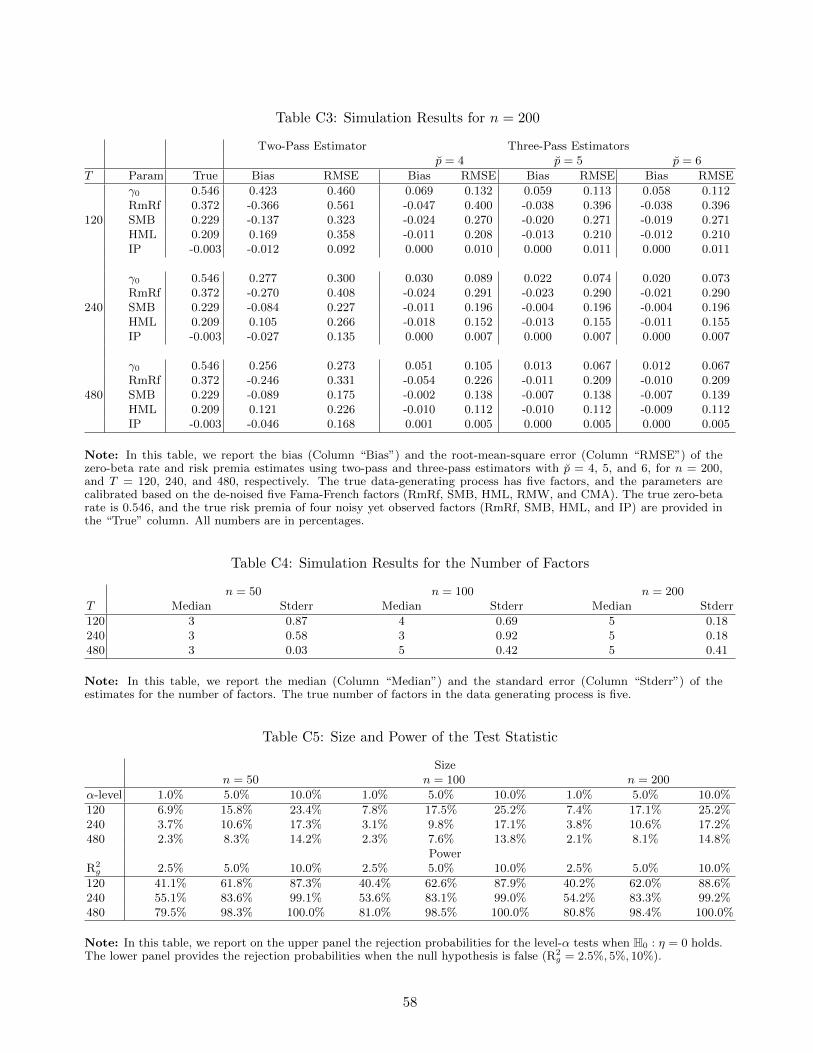
Table C3: Simulation Results for n = 200
Two-Pass Estimator Three-Pass Estimatorsp = 4 p = 5 p = 6
T Param True Bias RMSE Bias RMSE Bias RMSE Bias RMSE
γ0 0.546 0.423 0.460 0.069 0.132 0.059 0.113 0.058 0.112RmRf 0.372 -0.366 0.561 -0.047 0.400 -0.038 0.396 -0.038 0.396
120 SMB 0.229 -0.137 0.323 -0.024 0.270 -0.020 0.271 -0.019 0.271HML 0.209 0.169 0.358 -0.011 0.208 -0.013 0.210 -0.012 0.210IP -0.003 -0.012 0.092 0.000 0.010 0.000 0.011 0.000 0.011
γ0 0.546 0.277 0.300 0.030 0.089 0.022 0.074 0.020 0.073RmRf 0.372 -0.270 0.408 -0.024 0.291 -0.023 0.290 -0.021 0.290
240 SMB 0.229 -0.084 0.227 -0.011 0.196 -0.004 0.196 -0.004 0.196HML 0.209 0.105 0.266 -0.018 0.152 -0.013 0.155 -0.011 0.155IP -0.003 -0.027 0.135 0.000 0.007 0.000 0.007 0.000 0.007
γ0 0.546 0.256 0.273 0.051 0.105 0.013 0.067 0.012 0.067RmRf 0.372 -0.246 0.331 -0.054 0.226 -0.011 0.209 -0.010 0.209
480 SMB 0.229 -0.089 0.175 -0.002 0.138 -0.007 0.138 -0.007 0.139HML 0.209 0.121 0.226 -0.010 0.112 -0.010 0.112 -0.009 0.112IP -0.003 -0.046 0.168 0.001 0.005 0.000 0.005 0.000 0.005
Note: In this table, we report the bias (Column “Bias”) and the root-mean-square error (Column “RMSE”) of thezero-beta rate and risk premia estimates using two-pass and three-pass estimators with p = 4, 5, and 6, for n = 200,and T = 120, 240, and 480, respectively. The true data-generating process has five factors, and the parameters arecalibrated based on the de-noised five Fama-French factors (RmRf, SMB, HML, RMW, and CMA). The true zero-betarate is 0.546, and the true risk premia of four noisy yet observed factors (RmRf, SMB, HML, and IP) are provided inthe “True” column. All numbers are in percentages.
Table C4: Simulation Results for the Number of Factors
n = 50 n = 100 n = 200T Median Stderr Median Stderr Median Stderr
120 3 0.87 4 0.69 5 0.18240 3 0.58 3 0.92 5 0.18480 3 0.03 5 0.42 5 0.41
Note: In this table, we report the median (Column “Median”) and the standard error (Column “Stderr”) of theestimates for the number of factors. The true number of factors in the data generating process is five.
Table C5: Size and Power of the Test Statistic
Sizen = 50 n = 100 n = 200
α-level 1.0% 5.0% 10.0% 1.0% 5.0% 10.0% 1.0% 5.0% 10.0%
120 6.9% 15.8% 23.4% 7.8% 17.5% 25.2% 7.4% 17.1% 25.2%240 3.7% 10.6% 17.3% 3.1% 9.8% 17.1% 3.8% 10.6% 17.2%480 2.3% 8.3% 14.2% 2.3% 7.6% 13.8% 2.1% 8.1% 14.8%
PowerR2
g 2.5% 5.0% 10.0% 2.5% 5.0% 10.0% 2.5% 5.0% 10.0%
120 41.1% 61.8% 87.3% 40.4% 62.6% 87.9% 40.2% 62.0% 88.6%240 55.1% 83.6% 99.1% 53.6% 83.1% 99.0% 54.2% 83.3% 99.2%480 79.5% 98.3% 100.0% 81.0% 98.5% 100.0% 80.8% 98.4% 100.0%
Note: In this table, we report on the upper panel the rejection probabilities for the level-α tests when H0 : η = 0 holds.The lower panel provides the rejection probabilities when the null hypothesis is false (R2
g = 2.5%, 5%, 10%).
58
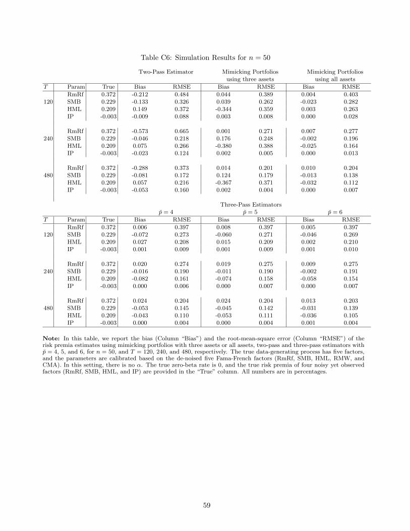
Table C6: Simulation Results for n = 50
Two-Pass Estimator Mimicking Portfolios Mimicking Portfoliosusing three assets using all assets
T Param True Bias RMSE Bias RMSE Bias RMSE
RmRf 0.372 -0.212 0.484 0.044 0.389 0.004 0.403120 SMB 0.229 -0.133 0.326 0.039 0.262 -0.023 0.282
HML 0.209 0.149 0.372 -0.344 0.359 0.003 0.263IP -0.003 -0.009 0.088 0.003 0.008 0.000 0.028
RmRf 0.372 -0.573 0.665 0.001 0.271 0.007 0.277240 SMB 0.229 -0.046 0.218 0.176 0.248 -0.002 0.196
HML 0.209 0.075 0.266 -0.380 0.388 -0.025 0.164IP -0.003 -0.023 0.124 0.002 0.005 0.000 0.013
RmRf 0.372 -0.288 0.373 0.014 0.201 0.010 0.204480 SMB 0.229 -0.081 0.172 0.124 0.179 -0.013 0.138
HML 0.209 0.057 0.216 -0.367 0.371 -0.032 0.112IP -0.003 -0.053 0.160 0.002 0.004 0.000 0.007
Three-Pass Estimatorsp = 4 p = 5 p = 6
T Param True Bias RMSE Bias RMSE Bias RMSE
RmRf 0.372 0.006 0.397 0.008 0.397 0.005 0.397120 SMB 0.229 -0.072 0.273 -0.060 0.271 -0.046 0.269
HML 0.209 0.027 0.208 0.015 0.209 0.002 0.210IP -0.003 0.001 0.009 0.001 0.009 0.001 0.010
RmRf 0.372 0.020 0.274 0.019 0.275 0.009 0.275240 SMB 0.229 -0.016 0.190 -0.011 0.190 -0.002 0.191
HML 0.209 -0.082 0.161 -0.074 0.158 -0.058 0.154IP -0.003 0.000 0.006 0.000 0.007 0.000 0.007
RmRf 0.372 0.024 0.204 0.024 0.204 0.013 0.203480 SMB 0.229 -0.053 0.145 -0.045 0.142 -0.031 0.139
HML 0.209 -0.043 0.110 -0.053 0.111 -0.036 0.105IP -0.003 0.000 0.004 0.000 0.004 0.001 0.004
Note: In this table, we report the bias (Column “Bias”) and the root-mean-square error (Column “RMSE”) of therisk premia estimates using mimicking portfolios with three assets or all assets, two-pass and three-pass estimators withp = 4, 5, and 6, for n = 50, and T = 120, 240, and 480, respectively. The true data-generating process has five factors,and the parameters are calibrated based on the de-noised five Fama-French factors (RmRf, SMB, HML, RMW, andCMA). In this setting, there is no α. The true zero-beta rate is 0, and the true risk premia of four noisy yet observedfactors (RmRf, SMB, HML, and IP) are provided in the “True” column. All numbers are in percentages.
59

Table C7: Simulation Results for n = 100
Two-Pass Estimator Mimicking Portfolios Mimicking Portfoliosusing three assets using all assets
T Param True Bias RMSE Bias RMSE Bias RMSE
RmRf 0.372 -0.228 0.478 0.047 0.395 0.015 0.417120 SMB 0.229 -0.114 0.315 0.070 0.272 -0.008 0.321
HML 0.209 0.109 0.347 -0.417 0.433 0.004 0.439IP -0.003 -0.010 0.098 0.002 0.008 0.000 0.073
RmRf 0.372 -0.223 0.377 0.043 0.283 -0.002 0.287240 SMB 0.229 -0.141 0.255 0.117 0.222 -0.010 0.202
HML 0.209 0.220 0.328 -0.348 0.353 -0.001 0.181IP -0.003 -0.024 0.114 0.002 0.006 0.000 0.020
RmRf 0.372 -0.301 0.373 0.030 0.202 0.001 0.205480 SMB 0.229 -0.095 0.177 0.083 0.156 -0.006 0.139
HML 0.209 0.173 0.252 -0.389 0.393 -0.002 0.117IP -0.003 -0.049 0.147 0.002 0.004 0.000 0.009
Three-Pass Estimatorsp = 4 p = 5 p = 6
T Param True Bias RMSE Bias RMSE Bias RMSE
RmRf 0.372 0.009 0.396 0.019 0.397 0.017 0.397120 SMB 0.229 -0.016 0.268 -0.018 0.269 -0.016 0.269
HML 0.209 0.000 0.208 -0.013 0.211 -0.012 0.212IP -0.003 0.000 0.010 0.000 0.011 0.000 0.011
RmRf 0.372 0.007 0.285 -0.005 0.285 -0.002 0.285240 SMB 0.229 -0.034 0.198 -0.018 0.196 -0.016 0.196
HML 0.209 0.003 0.148 0.003 0.149 -0.003 0.149IP -0.003 0.000 0.007 0.000 0.007 0.000 0.007
RmRf 0.372 0.008 0.204 0.004 0.204 0.001 0.204480 SMB 0.229 -0.030 0.140 -0.016 0.138 -0.012 0.138
HML 0.209 -0.003 0.107 -0.004 0.108 -0.004 0.108IP -0.003 0.000 0.004 0.000 0.005 0.000 0.005
Note: In this table, we report the bias (Column “Bias”) and the root-mean-square error (Column “RMSE”) of therisk premia estimates using mimicking portfolios with three assets or all assets, two-pass and three-pass estimators withp = 4, 5, and 6, for n = 100, and T = 120, 240, and 480, respectively. The true data-generating process has five factors,and the parameters are calibrated based on the de-noised five Fama-French factors (RmRf, SMB, HML, RMW, andCMA). In this setting, there is no α. The true zero-beta rate is 0, and the true risk premia of four noisy yet observedfactors (RmRf, SMB, HML, and IP) are provided in the “True” column. All numbers are in percentages.
60

Table C8: Simulation Results for n = 200
Two-Pass Estimator Mimicking Portfolios Mimicking Portfoliosusing three assets using all assets
T Param True Bias RMSE Bias RMSE Bias RMSE
RmRf 0.372 -0.357 0.554 0.022 0.396 NA NA120 SMB 0.229 -0.074 0.302 0.088 0.280 NA NA
HML 0.209 0.083 0.327 -0.386 0.400 NA NAIP -0.003 -0.009 0.087 0.003 0.008 NA NA
RmRf 0.372 -0.344 0.459 0.059 0.285 0.000 0.293240 SMB 0.229 -0.095 0.229 0.033 0.191 -0.003 0.227
HML 0.209 0.122 0.266 -0.382 0.388 -0.008 0.297IP -0.003 -0.026 0.130 0.002 0.006 0.002 0.051
RmRf 0.372 -0.276 0.351 0.030 0.201 0.000 0.202480 SMB 0.229 -0.097 0.180 0.088 0.158 -0.005 0.142
HML 0.209 0.068 0.201 -0.419 0.422 -0.003 0.127IP -0.003 -0.060 0.188 0.002 0.004 0.000 0.014
Three-Pass Estimatorsp = 4 p = 5 p = 6
T Param True Bias RMSE Bias RMSE Bias RMSE
RmRf 0.372 -0.017 0.401 -0.005 0.402 -0.005 0.402120 SMB 0.229 -0.005 0.273 -0.008 0.274 -0.008 0.274
HML 0.209 0.003 0.212 -0.012 0.214 -0.012 0.214IP -0.003 0.001 0.010 0.000 0.011 0.000 0.011
RmRf 0.372 0.001 0.284 0.001 0.284 0.001 0.284240 SMB 0.229 -0.010 0.193 -0.008 0.194 -0.008 0.194
HML 0.209 -0.009 0.149 -0.010 0.150 -0.010 0.151IP -0.003 0.000 0.007 0.000 0.007 0.000 0.007
RmRf 0.372 0.024 0.203 0.002 0.201 0.001 0.201480 SMB 0.229 -0.031 0.141 -0.008 0.138 -0.008 0.139
HML 0.209 -0.032 0.110 -0.009 0.107 -0.009 0.107IP -0.003 0.000 0.005 0.000 0.005 0.000 0.005
Note: In this table, we report the bias (Column “Bias”) and the root-mean-square error (Column “RMSE”) of therisk premia estimates using mimicking portfolios with three assets or all assets, two-pass and three-pass estimators withp = 4, 5, and 6, for n = 200, and T = 120, 240, and 480, respectively. The true data-generating process has five factors,and the parameters are calibrated based on the de-noised five Fama-French factors (RmRf, SMB, HML, RMW, andCMA). In this setting, there is no α. The true zero-beta rate is 0, and the true risk premia of four noisy yet observedfactors (RmRf, SMB, HML, and IP) are provided in the “True” column. All numbers are in percentages. NA meansthe estimators are “infeasible.”
61
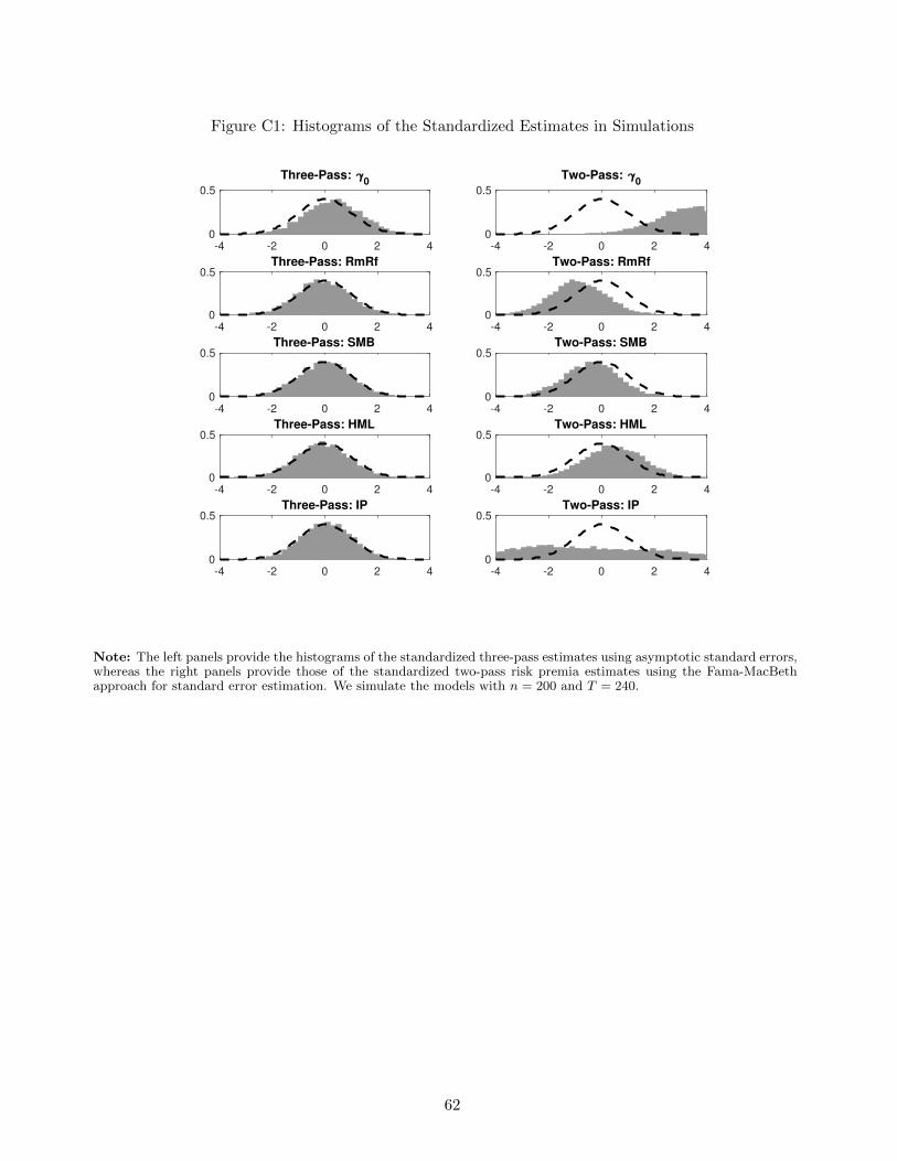
Figure C1: Histograms of the Standardized Estimates in Simulations
-4 -2 0 2 4
0
0.5
Three-Pass: 0
-4 -2 0 2 4
0
0.5
Three-Pass: RmRf
-4 -2 0 2 4
0
0.5
Three-Pass: SMB
-4 -2 0 2 4
0
0.5
Three-Pass: HML
-4 -2 0 2 4
0
0.5
Three-Pass: IP
-4 -2 0 2 4
0
0.5
Two-Pass: 0
-4 -2 0 2 4
0
0.5
Two-Pass: RmRf
-4 -2 0 2 4
0
0.5
Two-Pass: SMB
-4 -2 0 2 4
0
0.5
Two-Pass: HML
-4 -2 0 2 4
0
0.5
Two-Pass: IP
Note: The left panels provide the histograms of the standardized three-pass estimates using asymptotic standard errors,whereas the right panels provide those of the standardized two-pass risk premia estimates using the Fama-MacBethapproach for standard error estimation. We simulate the models with n = 200 and T = 240.
62

Figure C2: Histograms of the Standardized Estimates in Simulations
-4 -2 0 2 4
0
0.5
Three-Pass: RmRf
-4 -2 0 2 4
0
0.5
Three-Pass: SMB
-4 -2 0 2 4
0
0.5
Three-Pass: HML
-4 -2 0 2 4
0
0.5
Three-Pass: IP
-4 -2 0 2 4
0
0.5
Two-Pass: RmRf
-4 -2 0 2 4
0
0.5
Two-Pass: SMB
-4 -2 0 2 4
0
0.5
Two-Pass: HML
-4 -2 0 2 4
0
0.5
Two-Pass: IP
-4 -2 0 2 4
0
0.5
MP: RmRf
-4 -2 0 2 4
0
0.5
MP: SMB
-4 -2 0 2 4
0
0.5
MP: HML
-4 -2 0 2 4
0
0.5
MP: IP
-4 -2 0 2 4
0
0.5
MP3: RmRf
-4 -2 0 2 4
0
0.5
MP3: SMB
-4 -2 0 2 4
0
0.5
MP3: HML
-4 -2 0 2 4
0
0.5
MP3: IP
Note: The top panel plots the histograms of the standardized estimates using the three-pass estimator (top left) and thetwo-pass estimator (top right), respectively, for four parameters. The bottom panels provide those of the standardizedmimicking portfolio estimators, using three (bottom left) or all assets (bottom right), respectively. We simulate themodels with n = 200 and T = 240.
63

D Mathematical Proofs
D.1 Proofs of Main Theorems
Proof of Proposition 1. Given the weights of the mimicking portfolios, and by Assumptions A.1 and
A.2, these portfolio returns, i.e., rt = wᵀrt, satisfy the following factor model:
rt = βγ + βvt + ut, (D.3)
where β = wᵀβ, ut = wᵀut. Conditioning on β, the bias of the factor mimicking-portfolio estimator is:
γMPg − ηγ = ηΣvβᵀ(Σr)−1βγ − ηγ + Σz,u(Σr)−1βγ,
where Σz,u = Σz,uw and Σr = wᵀΣrw.
Because of (D.3), we have Σr = βΣvβᵀ + Σu, so that by Woodbury matrix identity
(Σr)−1 =(Σu)−1 − (Σu)−1β(βᵀ(Σu)−1β + (Σv)−1
)−1βᵀ(Σu)−1,
βᵀ(Σr)−1β =βᵀ(Σu)−1β − βᵀ(Σu)−1β(βᵀ(Σu)−1β + (Σv)−1
)−1βᵀ(Σu)−1β.
This further implies that (βᵀ(Σr)−1β
)−1=(βᵀ(Σu)−1β
)−1+ Σv,
where we use the fact that p ≥ p.Using this equation and by direct calculations, we obtain that
ηΣvβᵀ(Σr)−1βγ − ηγ =η
((Ip +
(βᵀ(Σu)−1β
)−1(Σv)−1
)−1
− Ip
)γ = −η (Ip +A)−1Aγ,
where A =(βᵀ(Σu)−1β
)−1(Σv)−1. We can then show that the maximum eigenvalue of A goes to zero
as n→∞, so the bias disappears asymptotically.
In fact, under Assumption A.3, λmax(Σu) = Op(snn−1), then
λmax(A) = λ−1min(Σvβᵀ(Σu)−1β) ≤ λ−1
min(Σv)λ−1min(βᵀβ)λmax(Σu) = Op(snn
−1).
By Weyl’s inequality, for any fixed ε > 0, with probability approaching 1
λmin(Ip +A) ≥ λmin(Ip) + λmin(A) > 1− ε.
It then follows that
‖ηΣvβᵀ(Σr)−1βγ − ηγ‖ ≤ ‖η‖‖γ‖λmax(A)λ−1min(Ip +A) = Op(snn
−1).
64
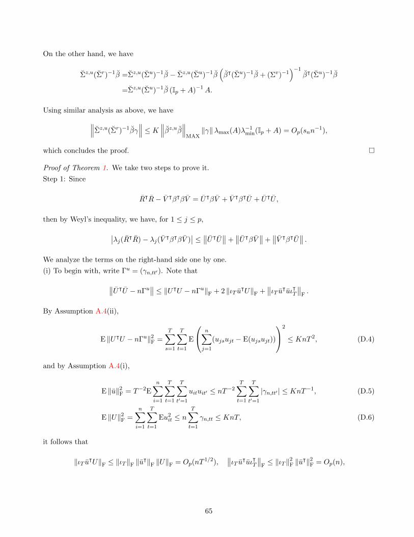
On the other hand, we have
Σz,u(Σr)−1β =Σz,u(Σu)−1β − Σz,u(Σu)−1β(βᵀ(Σu)−1β + (Σv)−1
)−1βᵀ(Σu)−1β
=Σz,u(Σu)−1β (Ip +A)−1A.
Using similar analysis as above, we have∥∥∥Σz,u(Σr)−1βγ∥∥∥ ≤ K ∥∥∥βz,uβ∥∥∥
MAX‖γ‖λmax(A)λ−1
min(Ip +A) = Op(snn−1),
which concludes the proof.
Proof of Theorem 1. We take two steps to prove it.
Step 1: Since
RᵀR− V ᵀβᵀβV = UᵀβV + V ᵀβᵀU + UᵀU ,
then by Weyl’s inequality, we have, for 1 ≤ j ≤ p,
∣∣λj(RᵀR)− λj(V ᵀβᵀβV )∣∣ ≤ ∥∥UᵀU
∥∥+∥∥UᵀβV
∥∥+∥∥V ᵀβᵀU
∥∥ .We analyze the terms on the right-hand side one by one.
(i) To begin with, write Γu = (γn,tt′). Note that
∥∥UᵀU − nΓu∥∥ ≤ ‖UᵀU − nΓu‖F + 2 ‖ιT uᵀU‖F +
∥∥ιT uᵀuιᵀT∥∥F.
By Assumption A.4(ii),
E ‖UᵀU − nΓu‖2F =T∑s=1
T∑t=1
E
n∑j=1
(ujsujt − E(ujsujt))
2
≤ KnT 2, (D.4)
and by Assumption A.4(i),
E ‖u‖2F = T−2E
n∑i=1
T∑t=1
T∑t′=1
uituit′ ≤ nT−2T∑t=1
T∑t′=1
|γn,tt′ | ≤ KnT−1, (D.5)
E ‖U‖2F =
n∑i=1
T∑t=1
Eu2it ≤ n
T∑t=1
γn,tt ≤ KnT, (D.6)
it follows that
‖ιT uᵀU‖F ≤ ‖ιT ‖F ‖uᵀ‖F ‖U‖F = Op(nT
1/2),∥∥ιT uᵀuιᵀT∥∥F
≤ ‖ιT ‖2F ‖uᵀ‖2F = Op(n),
65
and hence that
∥∥UᵀU − nΓu∥∥ = Op(n
1/2T ) +Op(nT1/2). (D.7)
Next, writing ρn,st = γn,st/√γn,ssγn,tt, by Assumption A.4(i) and the fact that |ρn,st| ≤ 1,
‖Γu‖2F =
T∑s=1
T∑t=1
γ2n,st =
T∑s=1
T∑t=1
γn,ssγn,ttρ2n,st
≤KT∑s=1
T∑t=1
|γn,ssγn,tt|1/2|ρn,st| ≤ KT∑s=1
T∑t=1
|γn,st| ≤ KT, (D.8)
so we have n ‖Γu‖ = Op(nT1/2). Therefore, we obtain
∥∥UᵀU∥∥ ≤ ∥∥UᵀU − nΓu
∥∥+ n ‖Γu‖ = Op(nT1/2) +Op(n
1/2T ). (D.9)
(ii) By Assumption A.7, we have
E ‖Uᵀβ‖2F =E
p∑j=1
T∑t=1
(n∑i=1
βijuit
)2
≤ KnT, (D.10)
E ‖uᵀβ‖2F =E
p∑k=1
(n∑i=1
uiβik
)2
≤ KnT−1, (D.11)
it follows that
∥∥Uᵀβ∥∥
F≤ ‖Uᵀβ‖F + ‖ιT ‖F ‖u
ᵀβ‖F = Op(n1/2T 1/2). (D.12)
Also, by Assumption A.5,
T−1∥∥V V ᵀ
∥∥MAX
≤∥∥T−1V V ᵀ − Σv
∥∥MAX
+ ‖Σv‖MAX + ‖vvᵀ‖MAX ≤ K, (D.13)
we have
∥∥V ∥∥ ≤ ∥∥V V ᵀ∥∥1/2 ≤ K
∥∥V V ᵀ∥∥1/2
MAX= Op(T
1/2). (D.14)
Therefore, we have
∥∥V ᵀβᵀU∥∥ =
∥∥UᵀβV∥∥ ≤ ∥∥Uᵀβ
∥∥F
∥∥V ∥∥ = Op(n1/2T ).
Combining (i) and (ii), we have for 1 ≤ j ≤ p,
n−1T−1∣∣λj(RᵀR)− λj(V ᵀβᵀβV )
∣∣ = Op(n−1/2 + T−1/2) = op(1). (D.15)
66
(iii) Moreover, by Assumption A.6, (D.14), and Weyl’s inequality again,∣∣∣n−1T−1λj(VᵀβᵀβV )− T−1λj(V
ᵀΣβV )∣∣∣ ≤ ∥∥∥n−1βᵀβ − Σβ
∥∥∥T−1∥∥V ᵀ
∥∥∥∥V ∥∥ = op(1),
and combined with Assumption A.5, and the fact that ‖v‖ ≤ K ‖v‖MAX = Op(T−1/2),∣∣∣∣T−1λj(V
ᵀΣβV )− λj((
Σβ)1/2
Σv(
Σβ)1/2
)∣∣∣∣≤∥∥T−1V V ᵀ − Σv
∥∥∥∥∥Σβ∥∥∥ ≤ (∥∥T−1V V ᵀ − Σv
∥∥+ ‖vvᵀ‖) ∥∥∥Σβ
∥∥∥ = op(1),
where we also use the fact that the non-zero eigenvalues of V ᵀΣβV are identical to the non-zero eigen-
values of(Σβ)1/2
V V ᵀ(Σβ)1/2
. Therefore, for 1 ≤ j ≤ p,∣∣∣∣n−1T−1λj(RᵀR)− λj
((Σβ)1/2
Σv(
Σβ)1/2
)∣∣∣∣ = op(1). (D.16)
Step 2: By Assumptions A.5 and A.6, there exists 0 < K1,K2 <∞, such that
K1 < λmin(Σv)λmin(Σβ) ≤ λmin(ΣvΣβ) ≤ λmax(ΣvΣβ) ≤ λmax(Σv)λmax(Σβ) < K2.
Therefore the eigenvalues of (Σβ)1/2Σv(Σβ)1/2 are bounded away from 0 and ∞, we have by (D.16), for
1 ≤ j ≤ p,
K1 < n−1T−1λj(RᵀR) < K2. (D.17)
On the other hand, we can write
RRᵀ = βV V ᵀβᵀ + U(IT − V ᵀ(V V ᵀ)−1V
)Uᵀ, (D.18)
where β = β+UV ᵀ(V V ᵀ)−1. By (4.3.2a) of Theorem 4.3.1 and (4.3.14) of Corollary 4.3.12 in Horn and
Johnson (2013), for p+ 1 ≤ j ≤ n, we have
λj(RRᵀ) ≤ λj−p
(U(IT − V ᵀ(V V ᵀ)−1V )Uᵀ)+ λp+1(βV V ᵀβ) ≤ λj−p(U Uᵀ) ≤ λ1(U Uᵀ).
Moreover, by (D.9), we have
λ1(U Uᵀ) =∥∥UᵀU
∥∥ = Op(nT1/2) +Op(n
1/2T ),
hence for p+ 1 ≤ j ≤ n, there exists some K > 0, such that
n−1T−1λj(RᵀR) ≤ K(n−1/2 + T−1/2). (D.19)
67

Now we define, for 1 ≤ j ≤ n,
f(j) = n−1T−1λj(RᵀR) + j × φ(n, T ).
(D.17) and (D.19) together imply that for 1 ≤ j ≤ p,
f(j)− f(p+ 1) =n−1T−1(λj(R
ᵀR)− λp+1(RᵀR))
+ (j − p− 1)φ(n, T )
>λj
((Σβ)1/2
Σv(
Σβ)1/2
)+ op(1) > K,
for some K > 0; and for p+ 1 < j ≤ n, we have
P(f(j) < f(p+ 1)) = P((j − p− 1)φ(n, T ) < n−1T−1
(λp+1(RᵀR)− λj(RᵀR)
))→ 0.
Therefore, p+ 1 = arg min1≤j≤p f(j) holds with probability approaching 1, and hence pp−→ p.
Proof of Theorem 2. Let Λ be the p × p diagonal matrix of the p largest eigenvalues of n−1T−1RᵀR.
We define a p× p matrix:
H = n−1T−1Λ−1V V ᵀβᵀβ. (D.20)
We have the following decomposition:
γ −Hγ =(βᵀβ
)−1βᵀ((β − βH
)γ + βv + u
)=Hv + n
(βᵀβ
)−1n−1
(H−ᵀβᵀu+H−ᵀβᵀ(β − βH)γ
+(β − βH−1)ᵀu+H−ᵀβᵀ(β − βH)v + (βᵀ −H−ᵀβᵀ)(β − βH)(γ + v)).
On the one hand, by Lemmas 4(b) and 4(e) we have
n−1∥∥∥βᵀβ −H−ᵀβᵀβH−1
∥∥∥MAX
≤∥∥∥n−1
(βᵀ −H−ᵀβᵀ
)(β − βH−1
)∥∥∥MAX
+ n−1∥∥∥H−ᵀβᵀ (β − βH−1
)∥∥∥MAX
+ n−1∥∥∥(β − βH−1
)ᵀβH−1
∥∥∥MAX
=Op(n−1 + T−1). (D.21)
Therefore, by Assumption A.6 and Lemma 4(a), (c), and (d), we have
γ −Hγ =Hv +Op(n−1 + T−1). (D.22)
On the other hand, we note that
η − ηH−1 = ηH−1(HV − V
)V ᵀ(V V ᵀ)−1 + ZV ᵀ(V V ᵀ)−1,
68

and by Lemma 5(a) and (b), we have
η − ηH−1 = T−1ZV ᵀHᵀ +Op(n−1 + T−1). (D.23)
Moreover, by Lemma 5(c), it follows that
∥∥η − ηH−1∥∥ = Op(n
−1 + T−1/2). (D.24)
Combining (D.22), (D.23), and Lemma 2, we obtain
γg − ηγ = ηv + T−1ZV ᵀ(Σv)−1γ +Op(n−1 + T−1).
Since
vec(T−1ZV ᵀ (Σv)−1 γ
)=(γᵀ (Σv)−1 ⊗ Id
) (vec(T−1ZV ᵀ) + vec(zvᵀ)
)=(γᵀ (Σv)−1 ⊗ Id
)vec(T−1ZV ᵀ) +Op(T
−1),
it follows from Assumption A.11 that
T 1/2
(T−1ZV ᵀ (Σv)−1 γ
ηv
)
L−→N
((0
0
),
( (γᵀ (Σv)−1 ⊗ Id
)Π11
((Σv)−1 γ ⊗ Id
) (γᵀ (Σv)−1 ⊗ Id
)Π12η
ᵀ
· ηΠ22ηᵀ
)).
Therefore, by the Delta method, and imposing T 1/2n−1 → 0, we obtain:
T 1/2(T−1ZV ᵀ (Σv)−1 γ + ηv
)L−→ N (0,Φ) ,
where Φ is given in the main text. This concludes the proof.
Proof of Theorem 3. We summarize the parameters of interest in Γ = (γ0 : (ηγ)ᵀ)ᵀ, and denote
Γ := (γ0, γᵀ)ᵀ =
((ιn : β)ᵀ(ιn : β)
)−1(ιn : β)ᵀr, Γ :=
(γ0
γg
):=
(1 0
0 η
)Γ =
(γ0
ηγ
).
Because β and η only rely on R and G, which do not depend on γ0ιn and α, we can recycle the estimates
derived in Lemmas 1 – 5, despite that the DGP is given by Assumption A.12 instead of Assumption
A.1.
We use the following decomposition:
Γ−
(γ0
Hγ
)
69
=(
(ιn : β)ᵀ(ιn : β))−1
(ιn : β)ᵀ((β − βH
)γ + βv + α+ u
)=
(0
Hv
)+
1
n
(ιᵀnιn ιᵀnβ
βᵀιn βᵀβ
)−11
n
(ιᵀnα
H−ᵀβᵀα
)+
1
n
(ιᵀnu+ ιᵀn(β − βH)γ
H−ᵀβᵀu+H−ᵀβᵀ(β − βH)γ
)
+1
n
(ιᵀn(β − βH)v
(β − βH−1)ᵀ(α+ u) +H−ᵀβᵀ(β − βH)v + (βᵀ −H−ᵀβᵀ)(β − βH)(γ + v)
). (D.25)
By Lemma 6(b), we have
n−1∥∥∥ιᵀn(β − βH−1)
∥∥∥MAX
= Op(n−1 + T−1).
Therefore, we have
1
n
(ιᵀnιn ιᵀnβ
βᵀιn βᵀβ
)=
1
n
(ιᵀnιn ιᵀnβH−1
H−ᵀβᵀιn H−ᵀβᵀβH−1
)+Op(n
−1 + T−1). (D.26)
Using this, and by Lemmas 2, 4, 5, 6, and 7, we have
Γ−
(γ0
ηγ
)=
(0
T−1ZV ᵀ(Σv)−1γ + ηv
)
+
(1 0
0 η
)1
n
(ιᵀnιn ιᵀnβ
βᵀιn βᵀβ
)+ op(1)
−1
×
1
n
(ιᵀnα
βᵀα
)+ op(n
−1/2 + T−1/2)
.
Moreover, by Cramer-Wold theorem and Lyapunov’s central limit theorem, we can obtain
n−1/2
(ιᵀnα
βᵀα
)L−→ N
((0
0
),
(1 βᵀ0β0 Σβ
)(σα)2
), (D.27)
where we use∥∥n−1βᵀιn − β0
∥∥MAX
= o(1) and∥∥n−1βᵀβ − Σβ
∥∥MAX
= o(1). Also, Assumptions A.6 and
A.13 ensure that (1− βᵀ0(Σβ)−1β0) and (Σβ − β0βᵀ0) are invertible. Therefore, by the Delta method, we
have
n1/2 (γ0 − γ0)L−→ N
(0,(
1− βᵀ0(Σβ)−1β0
)−1(σα)2
),
Similarly, we have
n1/2(
0 η) 1
n
(ιᵀnιn ιᵀnβ
βᵀιn βᵀβ
)+ op(1)
−1
× 1
n
(ιᵀnα
βᵀα
)L−→ N (0,Υ) ,
where
Υ = (σα)2η(
Σβ − β0βᵀ0
)−1ηᵀ.
70

By the same asymptotic independence argument as in the proof of Theorem 3 in Bai (2003), we establish
the desired result:
(T−1Φ + n−1Υ
)−1/2(γg − ηγ)
L−→ N (0, Id).
Proof of Theorem 4. By Assumptions A.5, A.6, and A.13, Lemma 4, (D.11), and (D.27), we have
n−1ιᵀnr = γ0 + βᵀ0γ +Op(n−1/2 + T−1/2),
n−1rᵀr = γᵀΣβγ + γ20 + (σα)2 + γᵀβ0γ0 + βᵀ0γγ0 +Op(n
−1/2 + T−1/2),
it then follows that
n−1rᵀMιn r = n−1rᵀr − (n−1ιᵀnr)2 = γᵀ(Σβ − β0β
ᵀ0)γ + (σα)2 + op(1).
On the other hand, by Assumption A.5, Lemma 3, (D.5), we have
n−1∥∥∥HᵀβᵀMιn r − βᵀMιn r
∥∥∥MAX
=∥∥∥(Hᵀβᵀ − βᵀ)Mιn(α+ βγ + βv + u)
∥∥∥MAX
≤n−1∥∥∥Hᵀβᵀ − βᵀ
∥∥∥F‖α+ βγ + βv + u‖F = Op(n
−1/2 + T−1/2).
Similarly, we have
n−1βᵀMιn r =(
Σβ − β0βᵀ0
)γ + op(1),
n−1βᵀMιnβ = Σβ − β0βᵀ0 + op(1),
therefore, we obtain
(n−1βᵀMιn r)ᵀ (n−1βᵀMιnβ
)−1 (n−1βᵀMιn r
)= γᵀ
(Σβ − β0β
ᵀ0
)γ + op(1),
which establishes R2v
p−→ R2v.
By Lemma 2, (D.48), (D.24) and the fact that ‖η‖MAX ≤ K, we have∥∥∥T−1ηV V ᵀηᵀ − ηΣvηᵀ∥∥∥
MAX
≤∥∥(η − ηH−1)(η − ηH−1)ᵀ
∥∥MAX
+∥∥(η − ηH−1)H−ᵀηᵀ
∥∥MAX
+∥∥ηH−1(η − ηH−1)ᵀ
∥∥MAX
+∥∥η(H−1H−ᵀ − Σv)ηᵀ
∥∥MAX
=Op(n−1/2 + T−1/2).
Also, by Assumptions A.5, A.8, and A.11, we have
T−1GGᵀ = T−1(ηV + Z)(ηV + Z)ᵀp−→ ηΣvηᵀ + Σz,
71

hence it follows that R2g
p−→ R2g.
Proof of Theorem 5. We denote the estimators of V and β based on p as V and β respectively. Without
loss of generality, we can assume p = p.
Consider the singular value decomposition of n−1/2T−1/2R by scaling (D.63), we have
n−1/2T−1/2ςᵀp+1:pR = Λ1/2p+1:pξ
ᵀp+1:p and n−1/2T−1/2Rξp+1:p = ςp+1:pΛ
1/2p+1:p, (D.28)
where Λp+1:p is a (p−p)×(p−p) diagonal matrix with the ith entry on the diagonal being n−1T−1λi(RᵀR),
ξp+1:p = (ξp+1 : ξp+2 : · · · : ξp) is T × (p− p), and ςp+1:p = (ςp+1 : ςp+2 : . . . : ςp) is n× (p− p). It is also
easy to observe that
V ᵀ =(V ᵀ : T 1/2ξp+1:p
), β =
(β : n1/2ςp+1:pΛ
1/2p+1:p
), V ξp+1:p = 0, and ςᵀp+1:pβ = 0.
Using the formula of block-diagonal matrix inversion, we can decompose
Γ− Γ =
(1
η
)1
n
(ιᵀnιn ιᵀnβ
βᵀιn βᵀβ
)−1
×
(−n−1ιᵀnςp+1:pΛ
1/2p+1:p∆
−1Λ1/2p+1:pς
ᵀp+1:p
(In − ιn(ιᵀnMβ
ιn)−1ιᵀnMβ
)r
0
)
+
(0
T−1/2n−1/2Gξp+1:p∆−1Λ
1/2p+1:pς
ᵀp+1:p
(In − ιn(ιᵀnMβ
ιn)−1ιᵀnMβ
)r
),
where ∆ = Λ1/2p+1:p
(Ip−p − ςᵀp+1:pιn(ιᵀnMβ
ιn)−1ιᵀnςp+1:p
)Λ
1/2p+1:p.
We analyze the right-hand side terms in the following. First, since Mββ = 0 and ςᵀp+1:pβ = 0, we
have
ςᵀp+1:p
(In − ιn(ιᵀnMβ
ιn)−1ιᵀnMβ
)r = ςᵀp+1:p
(In − ιn(ιᵀnMβ
ιn)−1ιᵀnMβ
)(α+ (β − βH)(v + γ) + u).
Since α is independent of ςp+1:p, we have
E∥∥∥ςᵀp+1:pα
∥∥∥2
F=
p−p∑j=1
E
(n∑i=1
ςp+1:p,ijαi
)2
= E ‖ςp+1:p‖2F (σα)2 ≤ K,
hence∥∥∥ςᵀp+1:pα
∥∥∥F
= Op(1). By Lemma 3(b) and (D.5), we have
∥∥∥ςᵀp+1:p(β − βH)∥∥∥ = Op(1 + n1/2T−1/2),
∥∥∥ςᵀp+1:pu∥∥∥ = Op(n
1/2T−1/2).
On the other hand, since by Lemma 7, (D.26), and (D.27), we have∥∥∥ιᵀnMβα∥∥∥ = Op(n
1/2), (ιᵀnMβιn)−1 = Op(n
−1).
72
By Lemmas 4 and 6, we have∥∥∥ιᵀnMβu∥∥∥ = Op(1 + nT−1),
∥∥∥ιᵀnMβ(β − βH)
∥∥∥ = Op(1 + nT−1).
Combined with Lemma 8, it implies that∥∥∥ςᵀp+1:pιn(ιᵀnMβιn)−1
(ιᵀnMβ
(α+ (β − βH)(v + γ) + u))∥∥∥ = op(1 + n1/2T−1).
With the above estimates, we obtain∥∥∥ςᵀp+1:p
(In − ιn(ιᵀnMβ
ιn)−1ιᵀnMβ
)r∥∥∥
≤∥∥∥ςᵀp+1:p(α+ (β − βH)(v + γ) + u)
∥∥∥+∥∥∥ςᵀp+1:pιn(ιᵀnMβ
ιn)−1(ιᵀnMβ
(α+ (β − βH)(v + γ) + u))∥∥∥
=Op(1 + n1/2T−1/2). (D.29)
Next, by Sherman-Morrison-Woodbury formula, we have∥∥∥Λ1/2p+1:p∆
−1Λ1/2p+1:p
∥∥∥ =
∥∥∥∥Ip−p + ςᵀp+1:pιnιᵀnςp+1:p
(ιᵀnMβ
ιn − ιᵀnςp+1:pςᵀp+1:pιn
)−1∥∥∥∥
=
∥∥∥∥Ip−p + n−1ςᵀp+1:pιnιᵀnςp+1:p
(1− n−1ιᵀnς1:pς
ᵀ1:pιn
)−1∥∥∥∥ ,
where we use the fact that
n−1ιᵀnMβιn = 1− n−1ιᵀnβ(βᵀβ)−1βᵀιn = 1− n−1ιᵀnς1:pς
ᵀ1:pιn.
By Lemma 8, for any p ≤ K, we have(1− n−1ιᵀnς1:pς
ᵀ1:pιn
)−1=(
1− n−1ιᵀnς1:pςᵀ1:pιn + op(1)
)−1=(
1− βᵀ0(Σβ)−1β0
)−1+ op(1).
Also,∥∥∥n−1ςᵀp+1:pιnι
ᵀnςp+1:p
∥∥∥ = op(1), which in turn leads to
∥∥∥Λ1/2p+1:p∆
−1Λ1/2p+1:p
∥∥∥ = Op(1). (D.30)
Combining (D.29), (D.30), and using Lemma 8 again, we have∥∥∥n−1ιᵀnςp+1:pΛ1/2p+1:p∆
−1Λ1/2p+1:pς
ᵀp+1:p
(In − ιn(ιᵀnMβ
ιn)−1ιᵀnMβ
)r∥∥∥ = op(n
−1/2 + T−1/2).
Next, by Lemmas 1 and 2,
∥∥ηV ξp+1:p
∥∥ =∥∥∥η(V −H−1V )ξp+1:p
∥∥∥ = Op(1 + n−1/2T 1/2).
By the independence of Z and ξp+1:p, we also have∥∥Zξp+1:p
∥∥ = Op(1). On the other hand, it follows
73

from (D.18) that
RRᵀ + U V ᵀ(V V ᵀ)−1V Uᵀ = U Uᵀ + βV V ᵀβᵀ,
where β = β + UV ᵀ(V V ᵀ)−1. By (4.3.2a) and (4.3.2b) of Theorem 4.3.1 in Horn and Johnson (2013),
for p+ 1 ≤ j ≤ p,
λj+p(U Uᵀ) + λn−1(βV V ᵀβᵀ) ≤ λj+p(RRᵀ + U V ᵀ(V V ᵀ)−1V Uᵀ) ≤ λj(RRᵀ) + λp+1(U V ᵀ(V V ᵀ)−1V Uᵀ).
Since rank(βV V ᵀβᵀ) ≤ p and rank(U V ᵀ(V V ᵀ)−1V Uᵀ) ≤ p, we obtain,
λp+p(U Uᵀ) ≤ λj+p(U Uᵀ) ≤ λj(RRᵀ) ≤ λj−p(U Uᵀ) ≤ λ1(U Uᵀ).
Since the empirical distribution of eigenvalues of T−1U Uᵀ follows the Marcenko-Pastur law (see, e.g.,
Theorem 3.6 in Bai and Silverstein (2009)), as n/T → c ∈ (0,∞), and this limiting law has a bounded
support, then there exist upper and lower bounds for finitely many largest eigenvalues
0 < K ′ ≤ T−1λj(RRᵀ) ≤ K, p+ 1 ≤ j ≤ p,
so that∥∥∥Λ−1/2p+1:p
∥∥∥ = Op(n1/2). We therefore obtain that
∥∥∥T−1/2n−1/2Gξp+1:p∆−1Λ
1/2p+1:pς
ᵀp+1:p
(In − ιn(ιᵀnMβ
ιn)−1ιᵀnMβ
)r∥∥∥
≤∥∥∥T−1/2n−1/2Gξp+1:p
∥∥∥∥∥∥Λ−1/2p+1:p
∥∥∥∥∥∥Λ1/2p+1:p∆
−1Λ1/2p+1:p
∥∥∥∥∥∥ςᵀp+1:p
(In − ιn(ιᵀnMβ
ιn)−1ιᵀnMβ
)r∥∥∥
=Op(n−1/2),
which concludes the proof.
Proof of Theorem 6. Again, we assume p = p. To prove the consistency of Φ, without loss of generality,
we focus on the case of Π12, and show that
(γᵀ ⊗ Id) Π12ηᵀ p−→
(γᵀ (Σv)−1 ⊗ Id
)Π12η
ᵀ. (D.31)
The proof for the other two terms in Φ is similar and hence is omitted.
Note that by (D.56), Lemma 2, Lemma 3(a), and Assumption A.5, we have∥∥∥T−1H−1V V ᵀH−ᵀ − Σv∥∥∥
MAX
=∥∥∥T−1H−1(V −HV )V ᵀH−ᵀ + T−1V (V ᵀ − V ᵀHᵀ)H−ᵀ + T−1V V ᵀ − Σv − vvᵀ
∥∥∥MAX
=Op(n−1 + T−1/2).
74

By (D.24), Lemma 2, and the proof of Theorem 2, we have
‖ηH − η‖MAX = Op(n−1 + T−1/2),
∥∥H−1γ − γ∥∥
MAX= Op(n
−1/2 + T−1/2). (D.32)
Therefore, to prove (D.31), we only need to show that
Π12 := (H−1 ⊗ Id)Π12H−ᵀ p−→ Π12, (D.33)
with which, and by the continuous mapping theorem, we have(γᵀ(
Σv)−1⊗ Id
)Π12η
ᵀ =
((H−1γ)ᵀ
(H−1ΣvH−ᵀ
)−1⊗ Id
)(H−1 ⊗ Id)Π12H
−ᵀ(ηH)ᵀ
p−→(γᵀ (Σv)−1 ⊗ Id
)Π12η
ᵀ.
Writing V = H−1V , we have
Π12,(i−1)d+j,i′ = vec(ejeᵀi )
ᵀ(H−1 ⊗ Id)Π12H−ᵀei′ = vec(eje
ᵀiH−1)ᵀΠ12H
−ᵀei′ = T−1T∑t=1
T∑s=1
zjtvitQtsvi′s,
where Qst =(
1− |s−t|q+1
)1|s−t|≤q.
In fact, to show (D.33), by Lemma 2 we only need to prove for any fixed 1 ≤ i, i′ ≤ p, and
1 ≤ j, j′ ≤ d,
Π12,(i−1)d+j,i′ − T−1T∑t=1
T∑s=1
zjtvitQtsvi′sp−→ 0, (D.34)
since by the identical proof of Theorem 2 in Newey and West (1987), we have
T−1T∑t=1
T∑s=1
zjtvitQtsvi′s −Π12,(i−1)d+j,i′p−→ 0.
Note that
the left-hand side of (D.34)
=T−1T∑t=1
T∑s=1
(zjt − zjt)(vit − vit)Qts(vi′s − vi′s) + (zjt − zjt)(vit − vit)Qtsvi′s
+ (zjt − zjt)vitQtsvi′s + zjt(vit − vit)Qtsvi′s + zjtvitQts(vi′s − vi′s).
We analyze these terms one by one. Since we have
Z − Z = ηV − ηV = (ηH−1 − η)HV − (η − ηH−1)(V −HV )− ηH−1(V −HV ), (D.35)
75

it follows from (D.24), (D.44), and Lemmas 1 and 2 that
T−1∥∥∥Z − Z∥∥∥
F
≤KT−1(∥∥ηH−1 − η
∥∥MAX
‖H‖∥∥V ∥∥
F+∥∥η − ηH−1
∥∥F
∥∥∥V −HV ∥∥∥F
+∥∥ηH−1
∥∥∥∥∥V −HV ∥∥∥F
)=Op(n
−1/2T−1/2 + T−1).
Moreover, by Lemma 9, Assumption A.16, (D.35), and (D.32), we have∥∥∥Z − Z∥∥∥MAX
≤∥∥ηH−1 − η
∥∥MAX
‖H‖∥∥V ∥∥
MAX+∥∥η − ηH−1
∥∥MAX
∥∥∥V −HV ∥∥∥MAX
+∥∥ηH−1
∥∥∥∥∥V −HV ∥∥∥MAX
=Op((log T )1/aT−1/2 + n−1/2T 1/4).
By Cauchy-Schwartz inequality, Lemmas 1, 9, and using the fact that |Qts| ≤ 1|t−s|≤q and∥∥vιᵀT∥∥F
=
‖v‖F∥∥ιᵀT∥∥F
≤ KT 1/2 ‖v‖MAX = Op(1), we have∣∣∣∣∣T−1T∑t=1
T∑s=1
(zjt − zjt)(vit − vit)Qts(vi′s − vi′s)
∣∣∣∣∣≤KqT−1
(∥∥∥V − V ∥∥∥MAX
+∥∥vιᵀT∥∥MAX
)(∥∥∥V − V ∥∥∥F
+∥∥vιᵀT∥∥F
)(∥∥∥Z − Z∥∥∥F
+∥∥zιᵀT∥∥F
)=Op
(q(T−1 + n−1)(T 1/4n−1/2 + T−1)
).
Similarly, because of∥∥∥V ∥∥∥
F≤ Op(T
1/2) implied by (D.45), ‖Z‖MAX = Op((log T )1/a) by Assumption
A.16 and Lemma 2, and by Assumptions A.5 and A.8, we have∣∣∣∣∣T−1T∑t=1
T∑s=1
(zjt − zjt)(vit − vit)Qtsvi′s
∣∣∣∣∣≤KqT−1 ‖V ‖MAX
(∥∥∥V − V ∥∥∥F
+∥∥vιᵀT∥∥F
)(∥∥∥Z − Z∥∥∥F
+∥∥zιᵀT∥∥F
)= Op
(q(log T )1/a(n−1 + T−1)
),∣∣∣∣∣T−1
T∑t=1
T∑s=1
(zjt − zjt)vitQtsvi′s
∣∣∣∣∣≤KqT−1 ‖V ‖MAX
∥∥∥V ∥∥∥F
(∥∥∥Z − Z∥∥∥F
+∥∥zιᵀT∥∥F
)= Op
(q(log T )1/a
(n−1/2 + T−1/2
)),∣∣∣∣∣T−1
T∑t=1
T∑s=1
zjt(vit − vit)Qtsvi′s
∣∣∣∣∣≤KqT−1 ‖Z‖MAX
∥∥∥V ∥∥∥F
(∥∥∥H−1V − V∥∥∥
F+∥∥vιᵀT∥∥F
)= Op
(q(log T )1/a
(n−1/2 + T−1/2
)),∣∣∣∣∣T−1
T∑t=1
T∑s=1
zjtvitQts(vi′s − vi′s)
∣∣∣∣∣≤KqT−1 ‖Z‖MAX
∥∥∥V ∥∥∥F
(∥∥∥H−1V − V∥∥∥
F+∥∥vιᵀT∥∥F
)= Op
(q(log T )1/a
(n−1/2 + T−1/2
)).
76
All the above terms converge to 0, as T, n → ∞, with qT−1/4 + qn−1/4 → 0 and n−3T → 0, which
establishes (D.34).
Finally, to show the consistency of Υ, we first note∥∥∥Hᵀ(
Σβ − β0βᵀ0
)H −
(Σβ − β0β
ᵀ0
)∥∥∥MAX
≤∥∥∥HᵀΣβH − Σβ
∥∥∥MAX
+∥∥∥Hᵀβ0β
ᵀ0H − β0β
ᵀ0
∥∥∥MAX
.
By Lemmas 2, 4(b), (e), and Assumption A.6,∥∥∥HᵀΣβH − Σβ∥∥∥
MAX
≤∥∥∥n−1HᵀβᵀβH − n−1βᵀβ
∥∥∥MAX
+∥∥∥n−1βᵀβ − Σβ
∥∥∥MAX
≤∥∥∥n−1
(Hᵀβᵀ − βᵀ
)(βH − β) + n−1
(Hᵀβᵀ − βᵀ
)β − n−1βᵀ(β − βH)
∥∥∥MAX
+ op(1)
=op(1). (D.36)∥∥∥Hᵀβ0βᵀ0H − β0β
ᵀ0
∥∥∥MAX
≤∥∥∥(Hᵀβ0 − β0
)(βᵀ0H − β
ᵀ0
)+ β0
(βᵀ0H − β
ᵀ0
)+(Hᵀβ0 − β0
)βᵀ0
∥∥∥MAX
=op(1),
where we also use Lemma 6(b):∥∥∥Hᵀβ0 − β0
∥∥∥MAX
= n−1∥∥∥(Hᵀβᵀ − βᵀ
)ιn
∥∥∥MAX
= op(1).
Next, by Lemma 3(b) and (D.32), we have
σα2 − (σα)2 =n−1
∥∥∥r − ιnγ0 − βγ∥∥∥2
F− (σα)2
=n−1∥∥∥ιn(γ0 − γ0) + βγ − βγ + βv + u
∥∥∥2
F+ n−1 ‖α‖2F − (σα)2
≤n−1 ‖ιn‖2F ‖γ0 − γ0‖2F + n−1 ‖β‖2F ‖v‖2F + n−1 ‖u‖2F + n−1
∥∥∥(βH − β)γ∥∥∥2
F
+ n−1∥∥∥(βH − β)(H−1γ − γ)
∥∥∥2
F+ n−1
∥∥β(H−1γ − γ)∥∥2
F+ op(1).
Therefore, by (D.24) and the continuous mapping theorem,
σα2ηHH−1
(Σβ − β0β
ᵀ0
)−1H−ᵀHᵀηᵀ
p−→ Υ,
which concludes the proof.
Proof of Theorem 7. By the conditioning argument, we assume p = p. By (D.23), we have
η − ηH−1 = T−1ZV ᵀHᵀ +Op(n−1 + T−1).
77

Therefore, when n−2T = o(1), we can rewrite:
W = T(ηH−1 + T−1ZV ᵀHᵀ) (Σ−1
v Π11Σ−1v
)−1 (ηH−1 + T−1ZV ᵀHᵀ)ᵀ + op(1).
Under H0 : η = 0, we have
W =(T−1/2ZV ᵀ
)(H−1Σ−1
v Π11Σ−1v H−ᵀ
)−1 (T−1/2ZV ᵀ
)ᵀ+ op(1).
By Assumption A.11, to show WL−→ χ2
p under H0, it is sufficient to establish that
H−1Σ−1v Π11Σ−1
v H−ᵀp−→ Π11.
By the same argument as in the proof of (D.33) and the fact that Σv = Id, we have
H−1Π11H−ᵀ p−→ Π11,
which leads to the first claim. The second claim is straightforward because H is invertible with proba-
bility approaching 1, ‖H‖ = Op(1) by Lemma 2, and T−1ZV ᵀ = Op(T−1/2) by Assumption A.8.
Proof of Theorem 8. For any 1 ≤ t ≤ T , we have
gt − ηvt = (η − ηH−1)(vt −Hvt) + (η − ηH−1)Hvt + ηH−1(vt −Hvt)− ηv (D.37)
By (D.43), we have
vt −Hvt =n−1T−1Λ−1(V −HV )(Uᵀβvt + Uᵀut
)+ n−1T−1Λ−1
(HV Uᵀβvt +HV Uᵀut
)+ n−1T−1Λ−1V V ᵀβᵀut. (D.38)
By Assumption B.17, we have ‖βᵀut‖ = Op(n1/2), so that using (D.11),
‖βᵀut‖F ≤ ‖βᵀut‖F + ‖βᵀu‖F = Op(n
1/2). (D.39)
By Assumption A.4(i), Assumptions A.15 and A.16, using the fact that |ρn,st| ≤ 1, we have
E ‖Uᵀut‖2F =E
T∑s=1
(nγn,st +
n∑k=1
(uksukt − E(uksukt))
)2
≤Kn2T∑s=1
γ2n,st +KnT ≤ n2
T∑s=1
|γn,st|+KnT = Kn2 +KnT,
E ‖ut‖2F ≤n∑k=1
Eu2kt ≤
n∑k=1
|σkk′ | ≤ K. (D.40)
78

Then from (D.5) and (D.57), it follows that
∥∥Uᵀut∥∥
F≤∥∥Uᵀu
∥∥F
+ ‖Uᵀut‖F + ‖ιT ‖F ‖uᵀ‖F ‖ut‖F = Op(n+ n1/2T 1/2).
The above estimates, along with (D.12), Lemma 1, and ‖vt‖ = Op(1), lead to∥∥∥n−1T−1Λ−1(V −HV )(Uᵀβvt + Uᵀut
)∥∥∥MAX
≤n−1T−1∥∥∥Λ−1
∥∥∥MAX
∥∥∥V −HV ∥∥∥F
(∥∥Uᵀβ∥∥
F‖vt‖+
∥∥Uᵀut∥∥
F
)= Op(n
−1 + T−1).
Moreover, it follows from (D.5), (D.50), and (D.55) that∥∥∥n−1T−1Λ−1(HV Uᵀβvt +HV Uᵀut
)∥∥∥MAX
≤Kn−1T−1∥∥∥Λ−1
∥∥∥MAX
‖H‖(∥∥V Uᵀβ
∥∥MAX
‖vt‖+∥∥V Uᵀ
∥∥F
(‖ut‖F + ‖u‖F))
=Op(n−1/2T−1/2 + T−1).
We thereby focus on the remaining term, which by Lemma 1, (D.14) and (D.39), satisfies
n−1T−1∥∥∥Λ−1V V ᵀβᵀut
∥∥∥MAX
≤ Kn−1T−1∥∥∥Λ−1
∥∥∥MAX
∥∥∥V ∥∥∥F
∥∥V ᵀ∥∥
F‖βᵀut‖MAX = Op(n
−1/2).
Therefore, we have
‖vt −Hvt‖MAX = Op(n−1/2 + T−1). (D.41)
Then by (D.37), (D.38), and (D.23), we have∥∥∥gt − ηvt − (T−1ZV ᵀHᵀHvt + n−1T−1ηH−1Λ−1V V ᵀβᵀut − ηv)∥∥∥
MAX= op(n
−1/2 + T−1/2).
Next, we note that by Assumption A.11 and Lemma 2,
T 1/2
(T−1vec
(ZV ᵀHᵀHvt
)ηv
)= T 1/2
((vᵀtH
ᵀH ⊗ Id)vec(ZV ᵀ)
ηv
)
L−→N
(0,
( (vᵀt (Σv)−1 ⊗ Id
)Π11
((Σv)−1 vt ⊗ Id
) (vᵀt (Σv)−1 ⊗ Id
)Π12η
ᵀ
· ηΠ22ηᵀ
)).
By (D.20) and Assumptions A.6 and B.17, we have
n−1/2T−1ηH−1Λ−1V V ᵀβᵀut =n1/2η(βᵀβ)−1βᵀutL−→ N
(0, η
(Σβ)−1
Ωt
(Σβ)−1
ηᵀ).
The desired result follows from the same asymptotic independence argument as in Bai (2003).
Proof of Theorem 9. For Ψ1t, we can follow exactly the same proof as that of Theorem 6, since, similar
79

to (D.32) for γ, we have the same estimate for vt by (D.41).
As to Ψ2t, similarly, we only need to show∥∥∥HᵀΩH − Ω∥∥∥
MAX= op(1).
Then by the continuous mapping theorem, along with (D.32) and (D.36), we have
Ψ2t = ηH(HᵀΣβH
)−1HᵀΩtH
(HᵀΣβH
)−1Hᵀηᵀ
p−→ Ψ2t.
Note that by Fan et al. (2013), we have∥∥∥Σu − Σu∥∥∥ = Op(snω
1−hT ). (D.42)
Then by (D.42) and Lemmas 3(b), 4(b), and using the fact that ‖β‖F = Op(n1/2) and ‖Σu‖ ≤ ‖Σu‖1 =
Op(sn), writing β = βH, we have
1
n
∥∥∥(β − β)ᵀ(Σu − Σu)(β − β)∥∥∥
MAX≤ 1
n
∥∥∥β − β∥∥∥2
F
∥∥∥Σu − Σu∥∥∥ = Op
(snω
1−hT (n−1 + T−1)
),
1
n
∥∥∥(β − β)ᵀΣu(β − β)∥∥∥
MAX≤ 1
n
∥∥∥β − β∥∥∥2
F‖Σu‖ = Op
(sn(n−1 + T−1)
),
1
n
∥∥∥βᵀ(Σu − Σu)β∥∥∥
MAX≤ 1
n‖β‖2F
∥∥∥Σu − Σu∥∥∥ = Op
(snω
1−hT
),
1
n
∥∥∥βᵀ(Σu − Σu)(β − β)∥∥∥
MAX≤ 1
n
∥∥∥(Σu − Σu)(β − β)βᵀ∥∥∥ ≤ 1
n
∥∥∥Σu − Σu∥∥∥∥∥∥βᵀ(β − β)
∥∥∥≤Kn
∥∥∥βᵀ(β − β)∥∥∥
MAX
∥∥∥Σu − Σu∥∥∥ = Op
(snω
1−hT (n−1 + T−1)
),
1
n
∥∥∥βᵀΣu(β − β)∥∥∥
MAX≤Kn
∥∥∥βᵀ(β − β)∥∥∥
MAX‖Σu‖ = Op
(sn(n−1 + T−1)
).
Therefore,∥∥∥HᵀΩH − Ω∥∥∥
MAX=
1
n
∥∥∥HᵀβᵀΣuβH − βᵀΣuβ∥∥∥
MAX
≤ 1
n
∥∥∥(β − β)ᵀ(Σu − Σu)(β − β) + (β − β)ᵀΣu(β − β)∥∥∥
MAX+
1
n
∥∥∥βᵀ(Σu − Σu)β∥∥∥
MAX
+1
n
∥∥∥βᵀ(Σu − Σu)(β − β) + (β − β)ᵀ(Σu − Σu)β∥∥∥
MAX+
1
n
∥∥∥βᵀΣu(β − β) + (β − β)ᵀΣuβ∥∥∥
MAX
=Op
(sn
(ω1−hT + n−1 + T−1
))= op(1),
which concludes the proof.
80

D.2 Technical Lemmas and Their Proofs
To prove the main theorems of the paper, we need the following lemmas:
Lemma 1. Under Assumptions A.1, A.2, A.4, A.5, A.6, and A.7, and suppose that p = p, we have∥∥∥V −HV ∥∥∥F
= Op(n−1/2T 1/2 + 1).
Proof. We make use of the following decomposition:
V −HV = n−1T−1(
Λ−1V RᵀR− Λ−1V V ᵀβᵀβV)
= n−1T−1Λ−1V(UᵀβV + V ᵀβᵀU + UᵀU
). (D.43)
Note that by (D.14), we have
∥∥V ∥∥F≤ K
∥∥V ∥∥ = Op(T1/2). (D.44)
Also, we have ∥∥∥V ∥∥∥ ≤ ∥∥∥V ∥∥∥F≤∥∥∥V V ᵀ
∥∥∥1/2
F= T 1/2. (D.45)
Using (D.17), we have ∥∥∥Λ∥∥∥
MAX= Op(1), and
∥∥∥Λ−1∥∥∥
MAX= Op(1). (D.46)
Combining these estimates with (D.12), we obtain
n−1T−1∥∥∥Λ−1V UᵀβV
∥∥∥F≤ Kn−1T−1
∥∥∥Λ−1∥∥∥
MAX
∥∥∥V ∥∥∥∥∥V Uᵀβ∥∥ = Op(n
−1/2T 1/2).
The same bound holds for another term:
n−1T−1∥∥∥Λ−1V V ᵀβᵀU
∥∥∥F
= Op(n−1/2T 1/2).
Using (D.9), (D.45), and (D.46), we obtain
n−1T−1∥∥∥Λ−1V UᵀU
∥∥∥F≤Kn−1T−1
∥∥∥Λ−1V UᵀU∥∥∥ ≤ K (n−1/2T 1/2 + 1
),
which concludes the proof.
Lemma 2. Under Assumptions A.1, A.2, A.4, A.5, A.6, and A.7, and suppose that p = p, if follows
that H is invertible with probability approaching 1. Moreover, ‖H‖ = Op(1),∥∥H−1
∥∥ = Op(1), and∥∥∥HᵀH − (Σv)−1∥∥∥ = Op(n
−1/2 + T−1/2).
81

Proof. Note that
∥∥V ∥∥ = Op(T1/2),
∥∥∥V ∥∥∥ ≤ ∥∥∥V ∥∥∥F
= T 1/2, n−1 ‖βᵀβ‖ ≤∥∥∥n−1βᵀβ − Σβ
∥∥∥+∥∥∥Σβ
∥∥∥ ≤ Op(1),
it follows from (D.20) that
‖H‖ ≤ n−1T−1∥∥∥V ∥∥∥∥∥V ∥∥ ‖βᵀβ‖∥∥∥Λ−1
∥∥∥ = Op(1).
Moreover, by triangle inequalities, Assumption A.5, and Lemma 1, we have
‖HΣvHᵀ − Ip‖ ≤∥∥HΣvHᵀ − T−1HV V ᵀHᵀ
∥∥+∥∥T−1HV V ᵀHᵀ − Ip
∥∥≤‖H‖2
(∥∥Σv − T−1V V ᵀ∥∥+ ‖vvᵀ‖
)+ T−1
∥∥∥V −HV ∥∥∥F
∥∥HV ∥∥+ T−1∥∥∥V ∥∥∥∥∥∥V −HV ∥∥∥
F
=Op(n−1/2 + T−1/2). (D.47)
By Weyl’s inequality, we have λmin(HΣvHᵀ) > 1/2 with probability approaching 1. This implies
that H(Σv)1/2 is invertible with probability approaching 1, so is H. Moreover, since λmin(HΣvHᵀ) ≤λmax(Σv) ‖H‖2, there exists ε > 0 such that ‖H‖ ≥ ε with probability approaching 1, and hence∥∥H−1
∥∥ = Op(1).
Multiplying H−1 and H−ᵀ from each side of (D.47) respectively, we obtain
∥∥Σv −H−1H−ᵀ∥∥ = Op(n
−1/2 + T−1/2), (D.48)
so that multiplying (Σv)−1 from the right hand side gives∥∥∥Ip −H−1H−ᵀ (Σv)−1∥∥∥ = Op(n
−1/2 + T−1/2).
Finally, multiplying HᵀH from the left gives the desired result.
Lemma 3. Under Assumptions A.1, A.2, A.4, A.5, A.6, A.7, A.8, A.9, and p = p, we have
(a) T−1∥∥∥(HV − V ) V ᵀ
∥∥∥MAX
= Op(n−1 + T−1).
(b)∥∥∥β − βH∥∥∥
F= Op(1 + n1/2T−1/2).
Proof. (a) By (D.43) and (D.46), we have∥∥∥(HV − V ) V ᵀ∥∥∥
MAX≤Kn−1T−1
∥∥∥V UᵀβV V ᵀ + V V ᵀβᵀU V ᵀ + V UᵀU V ᵀ∥∥∥
MAX.
(i) To bound the first term, we note that∥∥∥V Uᵀβ∥∥∥
MAX≤K
∥∥∥V −HV ∥∥∥F
∥∥Uᵀβ∥∥
F+K ‖H‖MAX
∥∥V Uᵀβ∥∥
MAX.
82

Since ‖v‖MAX = Op(T−1/2), it follows from (D.11) that
‖vuᵀβ‖MAX ≤ K ‖v‖MAX ‖uᵀβ‖MAX = Op(n
1/2T−1). (D.49)
Combining with Assumption A.9(ii), we have
∥∥V Uᵀβ∥∥
MAX≤ ‖V Uᵀβ‖MAX + T ‖vuᵀβ‖MAX = Op(n
1/2T 1/2). (D.50)
By Lemmas 1 and 2, (D.12), and (D.50), we obtain∥∥∥V Uᵀβ∥∥∥
MAX= Op(T + n1/2T 1/2). (D.51)
Therefore, by (D.13), we have∥∥∥V UᵀβV V ᵀ∥∥∥
MAX≤ K
∥∥∥V Uᵀβ∥∥∥
MAX
∥∥V V ᵀ∥∥
MAX= Op(T
2 + n1/2T 3/2).
(ii) To bound the second term, by Weyl’s inequalities and Assumption A.6,∣∣∣∣λmin
(1
nβᵀβ
)− λmin
(Σβ)∣∣∣∣ ≤∥∥∥∥ 1
nβᵀβ − Σβ
∥∥∥∥ = op(1).
Therefore, there exists some 0 < ε < λmin(Σβ), such that
λmin(βᵀβ) ≥ n(λmin(Σβ)− ε
),
which establishes that
∥∥(n−1βᵀβ)−1∥∥ = nλ−1
min(βᵀβ) = Op(1), (D.52)
so that∥∥∥V V ᵀ∥∥∥
MAX= nT
∥∥∥ΛH(βᵀβ)−1∥∥∥
MAX≤ KnT
∥∥∥Λ∥∥∥
MAX‖H‖MAX
∥∥(βᵀβ)−1∥∥ = Op(T ). (D.53)
Using (D.50) we have∥∥∥V V ᵀβᵀU V ᵀ∥∥∥
MAX≤ K
∥∥∥V V ᵀ∥∥∥
MAX
∥∥βᵀU V ᵀ∥∥
MAX= Op(n
1/2T 3/2).
(iii) Finally, we have∥∥∥V UᵀU V ᵀ∥∥∥
MAX≤∥∥∥(V −HV )UᵀU V ᵀ
∥∥∥MAX
+∥∥HV UᵀU V ᵀ
∥∥MAX
.
On the one hand, note that∥∥∥(V −HV )UᵀU V ᵀ∥∥∥
MAX≤ K
∥∥∥V −HV ∥∥∥F
∥∥UᵀU∥∥∥∥V ᵀ
∥∥83

Combining with (D.14), (D.9), and Lemma 1, we have∥∥∥(V −HV )UᵀU V ᵀ∥∥∥
MAX= Op(T
2 + nT ). (D.54)
On the other hand, we have
∥∥U V ᵀ∥∥
F≤ ‖UV ᵀ‖F + T ‖uvᵀ‖F .
By Assumption A.9(i):
E ‖UV ᵀ‖2F ≤p∑i=1
n∑j=1
E
(T∑t=1
vitujt
)2
≤ KnT.
Also, by Assumption A.5 and Equation (D.5),
‖v‖F ≤ p1/2 ‖v‖MAX = Op(T
−1/2), ‖u‖F = Op(n1/2T−1/2),
so that T ‖uvᵀ‖F = Op(n1/2), hence we obtain that
∥∥U V ᵀ∥∥
F= Op(n
1/2T 1/2), (D.55)
and that
∥∥HV UᵀU V ᵀ∥∥
MAX≤ K ‖H‖MAX
∥∥U V ᵀ∥∥2
F= Op(nT ).
Therefore, we obtain ∥∥∥V UᵀU V ᵀ∥∥∥
MAX= Op
(T 2 + nT
).
Combining (i), (ii), and (iii), we have
T−1∥∥∥(HV − V ) V ᵀ
∥∥∥MAX
= Op(n−1 + T−1).
To prove (b), using the following decomposition,
β − βH =− T−1(βH−1(HV − V )V ᵀH + U
(V ᵀ − V ᵀHᵀ
)H + U V ᵀHᵀH
),
it follows from Lemmas 1 and 2, (D.5), (D.6), (D.45), (D.55), and ‖β‖F ≤ p1/2 ‖β‖ = Op(n1/2), that
n−1∥∥∥β − βH∥∥∥
F≤Kn−1T−1 ‖β‖F
∥∥H−1∥∥
MAX
∥∥∥HV − V ∥∥∥F
∥∥∥V ᵀ∥∥∥
F‖H‖MAX
+Kn−1T−1∥∥U∥∥
F
∥∥∥V ᵀ − V ᵀHᵀ∥∥∥
F‖H‖MAX +Kn−1T−1
∥∥U V ᵀ∥∥
F‖H‖2MAX
=Op(n−1 + n−1/2T−1/2).
84

Lemma 4. Under Assumptions A.1, A.2, A.4, A.5, A.6, A.7, A.8, A.9, and p = p, we have
(a) n−1∥∥H−ᵀβᵀu∥∥
MAX= Op
(n−1/2T−1/2
).
(b) n−1∥∥∥H−ᵀβᵀ(β − βH)
∥∥∥MAX
= Op(n−1 + T−1
).
(c) n−1∥∥∥(β − βH−1
)ᵀu∥∥∥
MAX= Op(n
−1 + T−1).
(d) n−1∥∥∥H−ᵀβᵀ(β − βH)v
∥∥∥MAX
= Op(n−1T−1/2 + T−3/2).
(e) n−1∥∥∥(βᵀ −H−ᵀβᵀ)(β − βH)
∥∥∥MAX
= Op(n−1 + T−1).
Proof. For (a), by (D.11), we have
n−1∥∥H−ᵀβᵀu∥∥
MAX≤ Kn−1
∥∥H−1∥∥
MAX‖βᵀu‖F = Op
(n−1/2T−1/2
).
As to (b), we have
n−1H−ᵀβᵀ(β − βH)
=− n−1T−1(H−ᵀβᵀβH−1(HV − V )V ᵀH +H−ᵀβᵀU
(V ᵀ − V ᵀHᵀ
)H +H−ᵀβᵀU V ᵀHᵀH
).
(i) We need the following result, which can be shown by Lemmas 1 and 3:
T−1∥∥∥(HV − V )V ᵀ
∥∥∥MAX
≤T−1∥∥∥(HV − V )
(V ᵀ − V ᵀHᵀ
)∥∥∥MAX
+ T−1∥∥∥(HV − V )V ᵀHᵀ
∥∥∥MAX
≤KT−1∥∥∥V −HV ∥∥∥2
F+KT−1
∥∥∥(HV − V ) V ᵀ∥∥∥
MAX‖H‖MAX
=Op(n−1 + T−1). (D.56)
Combined with that ‖βᵀβ‖ = Op(n), we obtain
n−1T−1∥∥∥H−ᵀβᵀβH−1(HV − V )V ᵀH
∥∥∥ ≤ Kn−1 ‖βᵀβ‖T−1∥∥∥(HV − V )V ᵀ
∥∥∥MAX
= Op(n−1 + T−1).
(ii) It immediately follows from (D.12) and Lemma 2 that
∥∥H−ᵀβᵀU∥∥F
= Op(n1/2T 1/2).
Using this and Lemma 1, we have
n−1T−1∥∥∥H−ᵀβᵀU (V ᵀ − V ᵀHᵀ
)H∥∥∥
MAX≤n−1T−1
∥∥H−1βᵀU∥∥
F
∥∥∥V ᵀ − V ᵀHᵀ∥∥∥
F‖H‖F
=Op(n−1 + n−1/2T−1/2).
85

(iii) By (D.50) and Lemma 2, we have
n−1T−1∥∥H−ᵀβᵀU V ᵀHᵀH
∥∥MAX
≤ Kn−1T−1∥∥H−1
∥∥MAX
‖H‖2MAX
∥∥V Uᵀβ∥∥
MAX= Op(n
−1/2T−1/2).
(i), (ii), and (iii) yield (b).
To show (c), note that
n−1uᵀ(β − βH−1) =− n−1uᵀ(β − βH)H−1
=n−1T−1(uᵀβH−1(HV − V )V ᵀ + uᵀU
(V ᵀ − V ᵀHᵀ
)+ uᵀU V ᵀHᵀ
).
(iv) By (D.11), we have
‖uᵀβ‖F = Op(n1/2T−1/2).
Combined with (D.56), we have
n−1T−1∥∥∥uᵀβH−1(HV − V )V ᵀ
∥∥∥MAX
≤n−1T−1 ‖uᵀβ‖F∥∥H−1
∥∥MAX
∥∥∥(HV − V )V ᵀ∥∥∥
MAX
=Op
(n−3/2T−1/2 + n−1/2T−3/2
).
(v) Next, note that by (D.9)
∥∥uᵀU∥∥F
=T−1∥∥ιᵀTUᵀU
∥∥F
+ ‖ιT uᵀu‖F ≤ KT−1 ‖ιT ‖ ‖UᵀU‖+ ‖ιT ‖F ‖u
ᵀu‖MAX
=Op(n1/2T 1/2 + n). (D.57)
With this, we obtain
n−1T−1∥∥∥uᵀU (V ᵀ − V ᵀHᵀ
)∥∥∥MAX
≤n−1T−1∥∥uᵀU∥∥
F
∥∥∥V ᵀ − V ᵀHᵀ∥∥∥
F= Op
(n−1 + T−1
).
(vi) By (D.55), we have
n−1T−1∥∥uᵀU V ᵀ
∥∥MAX
≤ n−1T−1 ‖u‖F∥∥U V ᵀ
∥∥F
= Op(T−1).
(iv), (v), and (vi) yield (c).
As to (d), by Assumption A.5, Lemmas 2 and 4(b), we have
n−1∥∥∥H−ᵀβᵀ(β − βH)v
∥∥∥MAX
≤Kn−1∥∥∥H−ᵀβᵀ(β − βH)
∥∥∥MAX
‖v‖MAX = Op(n−1T−1/2 + T−3/2).
For (e), we use Lemmas 2 and 3(b):∥∥∥n−1(βᵀ −H−ᵀβᵀ)(β − βH)∥∥∥
MAX≤ n−1
∥∥∥β − βH∥∥∥2
F
∥∥H−1∥∥ = Op(n
−1 + T−1),
which concludes the proof.
86

Lemma 5. Under Assumptions A.1, A.2, A.4, A.5, A.6, A.7, A.8, A.9, A.10, and p = p, we have
(a)∥∥∥ηH−1
(HV − V
)V ᵀ(V V ᵀ)−1
∥∥∥MAX
= Op(n−1 + T−1).
(b) T−1∥∥∥(HV − V ) Zᵀ
∥∥∥MAX
= Op(n−1 + T−1).
(c)∥∥∥ZV ᵀHᵀ(V V ᵀ)−1
∥∥∥MAX
= Op(T−1/2).
Proof. To show (a), by (D.56) and the fact that T−1V V ᵀ = Ip, we have∥∥∥ηH−1(HV − V
)V ᵀ(V V ᵀ)−1
∥∥∥MAX
≤‖η‖MAX ‖H‖MAX
∥∥∥T−1(HV − V
)V ᵀ∥∥∥
MAX
=Op(n−1 + T−1).
For (b) we use the following decomposition∥∥∥(HV − V ) Zᵀ∥∥∥
MAX≤Kn−1T−1
∥∥∥V UᵀβV Zᵀ + V V ᵀβᵀU Zᵀ + V UᵀU Zᵀ∥∥∥
MAX.
(i) By Assumption A.8 and (D.51), we have∥∥∥V UᵀβV Zᵀ∥∥∥
MAX≤ K
∥∥∥V Uᵀβ∥∥∥
MAX(‖V Zᵀ‖MAX + T ‖v‖MAX ‖z‖MAX) = Op(T
3/2 + n1/2T ).
(ii) Next, since ‖z‖MAX = Op(T−1/2), it follows from (D.11) that
‖βᵀuzᵀ‖MAX ≤ ‖βᵀu‖MAX ‖z
ᵀ‖MAX = Op(n1/2T−1).
By Assumption A.10(ii), we have
E ‖βᵀUZᵀ‖2MAX ≤Kd∑l=1
p∑j=1
E
(T∑s=1
n∑k=1
zlsuksβkj
)2
= Op(nT ),
and hence
∥∥βᵀU Zᵀ∥∥
MAX≤ ‖βᵀUZᵀ‖MAX + T ‖βᵀuzᵀ‖MAX = Op(n
1/2T 1/2).
Therefore, we obtain∥∥∥V V ᵀβᵀU Zᵀ∥∥∥
MAX≤ K
∥∥∥V V ᵀ∥∥∥
MAX
∥∥βᵀU Zᵀ∥∥
MAX= Op(n
1/2T 3/2).
(iii) Finally, we note that∥∥∥V UᵀU Zᵀ∥∥∥
MAX≤∥∥∥(V −HV )UᵀU Zᵀ
∥∥∥MAX
+∥∥HV UᵀU Zᵀ
∥∥MAX
.
87
On the one hand, using the same argument as in the proof of (D.54) and∥∥Z∥∥ = Op(T
1/2), we obtain∥∥∥(V −HV )UᵀU Zᵀ∥∥∥
MAX= Op(T
2 + nT ). (D.58)
On the other hand, we have
∥∥U Zᵀ∥∥
F≤ ‖UZᵀ‖F + T ‖uzᵀ‖F .
By Assumption A.10(i):
E ‖UZᵀ‖2F ≤ Kd∑i=1
n∑j=1
E
(T∑t=1
zitujt
)2
= Op(nT ).
Also, by Assumption A.8 and Equation (D.5),
‖z‖F ≤ p1/2 ‖z‖MAX = Op(T
−1/2), ‖u‖F = Op(n1/2T−1/2),
so that T ‖uzᵀ‖F = Op(n1/2), hence we obtain
∥∥U Zᵀ∥∥
F= Op(n
1/2T 1/2). (D.59)
Combined with (D.55), we have
∥∥HV UᵀU Zᵀ∥∥
MAX≤ K ‖H‖MAX
∥∥U V ᵀ∥∥
F
∥∥U Zᵀ∥∥
F= Op(nT ).
Therefore, we obtain ∥∥∥V UᵀU Zᵀ∥∥∥
MAX= Op
(T 2 + nT
).
Combining (i), (ii), and (iii), we have
T−1∥∥∥(HV − V ) Zᵀ
∥∥∥MAX
= Op(n−1 + T−1).
For (c), by Lemma 2, Assumptions A.5 and A.8,∥∥∥ZV ᵀHᵀ(V V ᵀ)−1∥∥∥
MAX=∥∥T−1ZV ᵀHᵀ
∥∥MAX
≤∥∥T−1ZV ᵀHᵀ
∥∥MAX
+ ‖zvᵀHᵀ‖MAX = Op(T−1/2).
Lemma 6. Under Assumptions A.2, A.4, A.5, A.6, A.7, A.8, A.9, A.12, A.13, A.14, and p = p, we
have
(a) n−1 ‖ιᵀnu‖MAX = Op
(n−1/2T−1/2
).
88

(b) n−1∥∥∥ιᵀn(β − βH)
∥∥∥MAX
= Op(n−1 + T−1
).
(c)∥∥∥n−1ιᵀn(β − βH)v
∥∥∥MAX
= Op(n−1T−1/2 + T−3/2).
Proof. To show (a), we note that by Assumption A.14(ii),
E ‖ιᵀnUιT ‖2 ≤
T∑s=1
T∑s′=1
n∑i=1
n∑i′=1
|σii′,ss′ | ≤ KnT, (D.60)
so that
n−1 ‖ιᵀnu‖MAX = n−1T−1 ‖ιᵀnUιT ‖MAX = Op
(n−1/2T−1/2
).
To show (b), we start from the following decomposition:
n−1ιᵀn(β − βH) =− n−1T−1(ιᵀnβH
−1(HV − V )V ᵀH + ιᵀnU(V ᵀ − V ᵀHᵀ
)H + ιᵀnU V
ᵀHᵀH).
(i) By Assumption A.13, n−1 ‖ιᵀnβ‖∞ = Op(1). By Lemmas 1, 2, and 3, we have
n−1T−1∥∥∥ιᵀnβH−1(HV − V )V ᵀH
∥∥∥MAX
≤n−1T−1∥∥∥ιᵀnβH−1(HV − V )
(V ᵀ − V ᵀHᵀ
)H∥∥∥
MAX+ n−1T−1
∥∥∥ιᵀnβH−1(HV − V )V ᵀHᵀH∥∥∥
MAX
≤Kn−1T−1 ‖ιᵀnβ‖∞∥∥H−1
∥∥MAX
‖H‖MAX
∥∥∥V −HV ∥∥∥2
F
+Kn−1T−1 ‖ιᵀnβ‖∞∥∥H−1
∥∥MAX
∥∥∥(HV − V ) V ᵀ∥∥∥
MAX‖H‖2MAX
=Op(n−1 + T−1).
(ii) We note that
∥∥ιᵀnU∥∥F≤ ‖ιᵀnU‖F +
∥∥ιᵀnuιᵀT∥∥F,
and that by Assumption A.14(i),
E ‖ιᵀnU‖2F = E
T∑t=1
(n∑i=1
uit
)2
≤ KT∑t=1
n∑i=1
n∑i′=1
|σii′,t| ≤ KnT,
and that by Assumption A.14(ii) again,
E∥∥ιᵀnuιᵀT∥∥2
F≤ KT−1
n∑i=1
n∑i′=1
T∑t=1
T∑t′=1
|σii′,tt′ | ≤ Kn,
89

so that by Lemma 1 again, we obtain
n−1T−1∥∥∥ιᵀnU (V ᵀ − V ᵀHᵀ
)H∥∥∥
MAX≤ n−1T−1
∥∥ιᵀnU∥∥F
∥∥∥V ᵀ − V ᵀHᵀ∥∥∥
F‖H‖F
= Op(n−1 + n−1/2T−1/2).
(iii) By Assumption A.14(iii), we have
‖ιᵀnUV ᵀ‖MAX = Op
(n1/2T 1/2
). (D.61)
Moreover, it follows from (D.60) that
‖ιᵀnUιT vᵀ‖MAX ≤ ‖ιᵀnUιT ‖ ‖v‖MAX = Op(n
1/2), (D.62)
and hence that
∥∥ιᵀnU V ᵀ∥∥
MAX=∥∥ιᵀnUV ᵀ
∥∥MAX
≤ ‖ιᵀnUV ᵀ‖MAX + ‖ιᵀnUιT vᵀ‖MAX = Op(n1/2T 1/2).
Therefore, we have
n−1T−1∥∥ιᵀnU V ᵀHᵀH
∥∥MAX
= Op(n−1/2T−1/2).
Combining (i), (ii), and (iii) leads to (b).
To show (c), by Assumption A.5 and Lemma 6(b), we have
n−1∥∥∥ιᵀn(β − βH)v
∥∥∥MAX
≤ Kn−1∥∥∥ιᵀn(β − βH)
∥∥∥MAX
‖v‖MAX = Op(n−1T−1/2 + T−3/2),
which concludes the proof.
Lemma 7. Under Assumptions A.2, A.4, A.5, A.6, A.7, A.8, A.9, A.12, and p = p, we have
n−1∥∥∥(β − βH−1)ᵀα
∥∥∥MAX
= Op(n−1 + n−1/2T−1/2).
Proof. Note that
n−1αᵀ(β − βH−1) =− n−1αᵀ(β − βH)H−1
=n−1T−1(αᵀβH−1(HV − V )V ᵀ + αᵀU
(V ᵀ − V ᵀHᵀ
)+ αᵀU V ᵀHᵀ
).
Since α is i.i.d., and α and β are independent, we have
E ‖αᵀβ‖2F = E
p∑k=1
n∑j=1
αjβjk
2
≤ KE ‖β‖2F ≤ Kn,
90
and by (D.56), we obtain
n−1T−1∥∥∥αᵀβH−1(HV − V )V ᵀ
∥∥∥MAX
≤Kn−1T−1 ‖αᵀβ‖F∥∥H−1
∥∥MAX
∥∥∥(HV − V )V ᵀ∥∥∥
MAX
=Op(n−3/2 + n−1/2T−1).
Moreover, by Assumption A.12, we have
E ‖αᵀU‖2F =ET∑t=1
(n∑k=1
αkukt
)2
≤T∑t=1
n∑k=1
Eα2kEu
2kt ≤ KnT,
E ‖α‖2F ≤En∑k=1
α2k ≤ Kn.
Therefore, we obtain
∥∥αᵀuιᵀT∥∥
F≤‖α‖F ‖u‖F ‖ιT ‖F = Op(n).
These imply that
n−1T−1∥∥∥αᵀU
(V ᵀ − V ᵀHᵀ
)∥∥∥MAX
≤n−1T−1(‖αᵀU‖F +
∥∥αᵀuιᵀT∥∥
F
) ∥∥∥V ᵀ − V ᵀHᵀ∥∥∥
F
=Op(n−1 + n−1/2T−1/2).
Finally, by Assumption A.9(i), we have
E ‖αᵀUV ᵀ‖2F =n∑j=1
E(α2j )
p∑i=1
E
(T∑t=1
ujtvit
)2
≤ KnT.
Using the fact that
T ‖αᵀuvᵀ‖F ≤T ‖α‖F ‖u‖F ‖v‖F = Op(n),
we obtain
n−1T−1∥∥αᵀU V ᵀHᵀ
∥∥MAX
≤ n−1T−1 (‖αᵀUV ᵀ‖F + T ‖αᵀuvᵀ‖F) ‖H‖MAX = Op(n−1/2T−1/2).
Lemma 8. Under assumptions in the statement of Theorem 5, it holds that n−1/2ιᵀnςi+p = op(1), where
ςi+p is the ith left-singular vector of R, for i = 1, 2, . . . ,K, and K is finite.
Proof. Consider the singular value decomposition of R:
R =
min(n,T−1)∑i=1
λi(RᵀR)1/2ςiξ
ᵀi , (D.63)
91
where ςi and ξi are n× 1 and T × 1 singular vectors, respectively. Similarly, we have the singular value
decomposition of MβUMV ᵀ :
MβUMV ᵀ =
min(n,T−1)−p∑i=1
λi(MβUMV ᵀUᵀMβ)1/2ςiξᵀi .
Because Mβ
= Mς1:p and MV ᵀ = Mξᵀ1:p
, where we use the notation a1:p = (a1 : a2 : . . . : ap), it implies
that
MβRM
V ᵀ =
min(n,T−1)−p∑i=1
λi+p(RᵀR)1/2ςi+pξ
ᵀi+p, (D.64)
that is, for i = 1, 2, . . . ,min(n, T − 1) − p, the (i + p)th singular vectors and singular value of R are
identical to the ith singular vectors and singular values of MβRM
V ᵀ . Note that by simple calculations,
we have
MβUMV ᵀ = MβUMιTMV ᵀ = MβUM[ιT :V ᵀ].
Moreover, since Mβ and M[ιT :V ᵀ] are idempotent matrices with ranks being n − p and T − p − 1,
respectively, there exist n× (n− p) and T × (T − p− 1) matrices O1 and O2 such that
Mβ = O1Oᵀ1 , M[ιT :V ᵀ] = O2O
ᵀ2 , Oᵀ
1O1 = In−p, Oᵀ2O2 = IT−p−1.
Because vec(U) is an nT -dimensional vector of i.i.d. Gaussian variables independent of O1 and O2,
vec (Oᵀ1UO2) = (Oᵀ
2⊗Oᵀ1)vec(U) is an (n−p)(T −p−1)-dimensional vector of i.i.d. Gaussian variables.
Writing U = Oᵀ1UO2, the singular value decomposition of U is
U =
min(n,T−1)−p∑i=1
λ1/2i (U Uᵀ)ςiξ
ᵀi ,
it follows from Properties 1 and 4 of Bai and Silverstein (2009) that ςi and ξi are distributed uniformly
on n− p and T − p− 1 dimensional spheres, respectively. Using their Gaussian representation it follows
that
ςid=
Zn−p‖Zn−p‖
, and ξid=
ZT−p−1
‖ZT−p−1‖,
where Zk denotes standard Gaussian vectors of length k and “d=” means “equal in distribution.” Because
MβUMV ᵀ = O1UOᵀ2 , it follows that conditional on β,
ςi =O1ςid=O1Zn−p‖Zn−p‖
d=
O1Zn−p‖O1Zn−p‖
d=
MβZn‖MβZn‖
.
92

Because (n − p)−1/2 ‖MβZn‖a.s.−→ 1 and Var(ιᵀnMβZn) = E (ιᵀnMβιn) = O(n), it yields that for i =
1, 2, . . . ,min(n, T − 1)− p,
n−1/2ιᵀnςid= n−1/2 ι
ᵀnMβZn‖MβZn‖
= op(1).
Finally, by the same argument in the proof of Theorem 3.2 of Moon and Weidner (2015), we have for i =
1, 2, . . . ,K, ‖ςi+p − ςi‖ = op(1). This concludes the proof because n−1/2 ‖ιᵀn(ςi+p − ςi)‖ ≤ ‖ςi+p − ςi‖ =
op(1).
Lemma 9. Under Assumptions A.2, A.4, A.5, A.6, A.7, A.8, A.9, A.12, A.15, A.16, and p = p, we
have ∥∥∥V −HV ∥∥∥MAX
= Op
(n−1/2T 1/4 + T−1/2
).
Proof. By (D.43)
V −HV = n−1T−1Λ−1V(UᵀβV + V ᵀβᵀU + UᵀU
).
We bound each term on the right-hand side. First, note that by the exponential-tail condition,∥∥V ∥∥MAX
= Op((log T )1/a). Along with (D.51), we obtain∥∥∥V UᵀβV∥∥∥
MAX≤ K
∥∥∥V Uᵀβ∥∥∥
MAX
∥∥V ∥∥MAX
= Op
(T (log T )1/a + n1/2T 1/2(log T )1/a
).
Next, by Assumption A.16 and Bonferroni and Markov inequalities,
P(maxt≤T‖βᵀut‖ > x) ≤ T max
t≤TP(‖βᵀut‖ > x) ≤ Tx−4 max
t≤TE ‖βᵀut‖4 ≤ KTx−4n2,
which implies that
maxt≤T‖βᵀut‖ = Op(T
1/4n1/2).
Then by (D.11) and (D.53), we have∥∥βᵀuιᵀT∥∥MAX
= ‖βᵀu‖MAX = Op(n1/2T−1/2), and hence
∥∥∥V V ᵀβᵀU∥∥∥
MAX≤ K
∥∥∥V V ᵀ∥∥∥
MAX
(maxt≤T‖βᵀut‖+
∥∥βᵀuιᵀT∥∥MAX
)= Op
(n1/2T 5/4
).
Finally, by Cauchy-Schwartz inequality,
E ‖Uᵀut − E(Uᵀut)‖4F = E
(T∑s=1
(uᵀsut − E(uᵀsut))2
)2
≤ TT∑s=1
E(uᵀsut − E(uᵀsut))4 ≤ Kn2T 2,
93

therefore, by Bonferroni and Markov inequalities again, we have
P
(maxt≤T‖Uᵀut − E(Uᵀut)‖F > x
)≤ T max
t≤TP (‖Uᵀut − E(Uᵀut)‖F > x) ≤ KT 3x−4n2,
which implies that
maxt≤T‖Uᵀut − E(Uᵀut)‖F = Op(n
1/2T 3/4).
Also, by Assumption A.15 and the fact that |ρn,tt′ | ≤ 1, we obtain
maxt≤T‖E(Uᵀut)‖F = max
t≤T
(T∑t′=1
(E(uᵀtut′))2
)1/2
= nmaxt≤T
(T∑s=1
γ2n,tt′
)1/2
≤ Kn.
Since by (D.5), (D.57), and (D.40), we have
maxt≤T
∥∥Uᵀut∥∥
F≤∥∥Uᵀu
∥∥F
+ maxt≤T‖ιT ‖F ‖u
ᵀ‖F ‖ut‖F + maxt≤T‖Uᵀut − E(Uᵀut)‖F + max
t≤T‖E(Uᵀut)‖F
=Op(n1/2T 3/4 + n),
it follows that∥∥∥V UᵀU∥∥∥
MAX≤ K max
t≤T
∥∥∥V Uᵀut
∥∥∥ ≤ K ∥∥∥V ∥∥∥F
maxt≤T
∥∥Uᵀut∥∥
F= Op(n
1/2T 5/4 + nT 1/2).
This concludes the proof.
94