637

Asset Strategy for Defined Benefit Pension Schemes

Jon JWey and Shyam Mehta

Abstract Part one of this paper presents a brief review and critique of traditional actuarial approaches to pension fund asset liability strategy work. A first principles approach is adopted.

The second part of this paper asks and answers questions such as:

0 What factors influence optimal investment strategy? 0 How do shareholder and trustee viewpoints differ? 0 Do the minimum funding requirement (“MFR”) rules reduce the

attractiveness of equity investment?

In the third part of this paper, a mathematical model is presented to determine optimal investment in risky assets according to key inputs such as initial funding level, bankruptcy risk of the sponsor and the relationship between MFR and final salary liabilities. This should not be viewed as a definitive model as there are other influences such as tax and liquidity, also discussed in the paper, which have not been allowed for. However, the authors hope that this will provide a basis for the construction of new and better asset/liability models in the future. Section 9 presents a non mathematical summary of key results.

Part four summarises our conclusions.

Dans une premiere partie ce papier presente un court examen et une critique des approches actuarielles traditionelles utilisees pour detinir une allocation d ‘actifs en fonction du passif. L’approche des premiers principes est adopt&e.

Dans la seconde partie des questions sont posees avec les reponses, ainsi:

638

0 Quels sont les facteurs qui influencent une strategic d ‘investissement optimale?

0 Y-a-t-ils des conflits entre le point de vue de 1 ‘actionnaire et du “trustee”? 0 Les nouvelles dispositions en mat&e de financement minimum (MFR)

reduissent-elles 1 ‘attrait des placements en actions?

Nous presentons en troisitme partie, un modele mathematique pour determiner 1 ‘investissement optimal en actifs risques selon des facteurs clefs comme le montant initial de la contribution, le risque d’insolvabilid de sponsor et le lien entre le financement minimum et les salaires a verser en fin de pkiode. Ce modele ne doit pas &tre consider6 comme definitif car il existe d ‘awes influences mentionnks aussi darts le papier, comme la fkalite et la liquiditk qui n’ont pas etd pris en compte. Les auteurs espkrent neanmoins, qu’il constitutera une base pour l’elaboration d’un meilleur modele de determination d’une allocation d’actifs optimale dans l’avenir. La neuvitme section prtsente un sommaire non mathematique des principaux resultats.

La quatrieme partie resume nos conclusions.

Keywords

Pension, asset/liability-models, investment strategy.

Contact: Jon Exley, William M. Mercer, Wellington Plaza, 31 Wellington Street, Leeds LSl 4DL (United Kingdom); Tel: + 44-113-243 6671, Fax: + 44-113-244 9452.

639

Part I: A Critique of Current Actuarial Approaches

1. 1.1

2. 2.1

2.2

Introduction This part of our paper considers some of the foundations underlying most modem actuarial analyses of optimal ‘long term’ investment strategies, in relation to the conclusions reached by financial economic (and more traditional actuarial) theory.

The Time Diversification Effect Lockyer (1990), Clark (1992), Thorley (1995), amongst others, suggest that the risk of equity investment declines as the holding period increases, and that the ‘optimal’ level of equity investment is therefore an increasing function of time horizon. However, the validity of this risk reduction over time, which we will refer to as the ‘time diversification effect’, is by no means obvious, nor is it universally accepted.

The case in favour of the time diversification effect appears to rest on intuitive arguments such as:

(1) The Central Limit Theorem allows us to approximate terminal portfolio value (VT) using the normal distribution for logs of asset prices. The average outcome under this distribution increases in direct proportion to time t, while the standard deviation increases only with d(r).

(2) Equities exhibit high short term but lower long term volatility. It has been suggested that equities typically bounce back after a fall and that they tend towards some long term value. These effects are commonly referred to as mean reversion.

(3) Investors are thought to behave as if they believe in the effect.

Clearly, (3) ignores the possibility that observed behaviour can be attributed more rationally to alternative explanations (see Samuelson 1963). Part three of this paper discusses in detail one such alternative explanation.

Many studies have attempted to assess the second effect, mean reversion. The evidence for mean reversion and the twin concept of the predictability of dividend yields is mixed. For example, one recent study found no evidence to support (Goetzmann & Jorion (1995)) of long term returns in the UK and concluded that if anything the data was more consistent with a hypothesis of mean aversion. Other recent studies examined US data and could not reject the null hypothesis of no predictability (Nelson & Kim (1993) and Goetzmann & Jorion (1993)). Anecdotal evidence also casts some doubt on the validity of mean reversion. For some crises of confidence (the UK in 1974) markets recovered. In other cases (Germany during the first and second world wars), markets did not recover. It should perhaps be mentioned here that many actuarial models, including the Wilkie model incorporate equity mean reversion effects. For a fuller discussion of mean reversion and market

640

efficiency the reader is referred to Exley, Mehta and Smith (1996).

2.3 It would appear that the main case for time diversification is assertion (1). The argument can be illustrated by using a log normal process for the value V, of an equity portfolio at time f relative to the value of an investment in cash:

V, = Vgxp( p.t + a.d(t).Z ), where Z = N(O,l)

However, two very different conclusions can be drawn from this equation

(a) We can first choose a percentile probability p’ arbitrarily close to 100% and then show that for any V” we can find T, such that;

Prob( VT > v’ ) > p’.

(b) We can first choose an arbitrarily long time horizon T and then demonstrate that there always exists some v” such that;

Prob{ Vr<v”]>Prob( V,iV”],foranyr<T.

The first ordering suggests that the risk of failing to achieve any given target portfolio value (v’) reduces over time; the second ordering suggests that there is always some ‘catastrophic’ value (v”) for which the probability of this outcome is highest for the longest choice of holding period. Although essentially the basis of assertion (1) above, decision making based on conclusion (a) would ignore the value of large losses and focus only on their frequency.

2.4 Given that investors are risk averse, they are likely generally to place significant weight on the risk of catastrophic loss. The use of a given risk of ruin, or of a subjective choice of acceptable loss probabilities, has no regard to the amount of loss. For many applications both the amount of loss, and degree of risk aversion, are very important. It is therefore by no means clear whether (a) or (b) has the most significant effect on portfolio choice. This can be demonstrated by using some common utility functions. For example, Merton & Samuelson (1973) show that the frequently used utility function, - W” (l-x), exhibits no time diversification benefit.

2.5 Bodie (1995) adds to this argument by invoking option pricing (both empirical and theoretical). He observes that, if time diversification applied to the choice between equity or risk free investment, European put option prices (for a strike price equal to the initial stock price plus interest at the risk free rate) would decrease as the time horizon increased. In practice, observed option prices increase with the length of the time horizon (contradicting assertion (3)). This argument is also quite powerful from a theoretical perspective, since the mathematical arguments presented in favour of time diversification would, at first sight, appear to apply within a Black & Scholes (1973) environment, and yet clearly they do not. Further, as Bodie points out, the

2.6

3. 3.1

3.2

3.3

3.4

3.5

641

Black & Scholes approach applies for a range of mean reversion effects (contradicting assertion (2)).

These conclusions have profound implications for modem actuarial advice on portfolio selection and for choice of actuarial valuation basis. Conventional wisdom appears to be spurious. A main focus of this paper is to explore the rationale for pension fund equity investment in the absence of time diversification benefits.

The Cost Implications of Alternative Investment Strategies We consider here the argument that switching pension fund assets from equities to low risk assets such as fixed and index linked Government securities results in a measurable and substantial increase in the cost of pension provision equal to the equity risk premium, generally estimated in this context to be ‘realistically’ of the order of 1%-3% pa (see for example Wilkie, (1995) and Thornton & Wilson, (1992)).

The risk premium quoted above would in fact be regarded as a conservative estimate relative to empirical studies (Barclays de Zoete Wedd, (1995) and Ibbotson & Sinquefield, (1989)). which generally reveal a premium of the order of 6% pa or 8% pa relative to cash returns. There must be a suspicion that the actuarial estimate of this premium contains some subjective margin for ‘prudence’, or implicit risk adjustment.

However, such debate, while highlighting the difficulty of establishing ‘realistic’ estimates, maybe of no real consequence. As discussed by Smith (1996) the Modigliani-Miller theorem (1958) states that (in the absence of transaction costs) the value of a firm cannot be altered by reallocating the financial assets held. In other words, whatever the choice of risk premium, the risk adjusted ‘benefit’ of equity investment to shareholders is nil: the additional return achieved on equities is offset by the additional risk.

In the context of pension fund investment, this result can be verified by analogy with an investor holding a short position in a corporate bond, which we equate with a pension liability. It cannot be argued that the value of this short position (superficially similar to the market cost of the liability) can be reduced or increased by the investor reallocating his portfolio of assets to or from equities. If assets are traded at market value then, (absent transaction costs), portfolio value at any point in time (immediately before and after the trade) must be the same, regardless of the choice of allocation.

As suggested by Smith (1996), in order to establish costs and benefits associated with equity investment, we need to look more closely at ‘transaction costs’. This is confirmed by Leland (1994) who suggests the existence of an optimal capital structure for firms facing taxation and bankruptcy costs (two examples from the general heading of transaction effects).

3.6 These costs and benefits are likely to be of a significantly lower order of

4. 4.1

4.2

4.3

4.4

4.5

4.6

642

magnitude than the equity risk premium quoted above. However from first principles they are more likely candidates for influencing optimal pension fund investment strategies than conventional considerations of expected risk premium. We therefore discuss in detail in part three more subtle issues which arise when the above investor is also the issuer of the bond and his assets in part act as security against bankruptcy default.

Influence Of Actuarial Bases It is, important to examine whether the use of ‘actuarial’ rather than market values also gives rise to spurious effects and distorts asset/liability management.

By way of example of such effects, we can pursue our example of an investor with a short position in a corporate bond. The ‘matched’ position is a back to back position in the same bond. However, applying the concept of an ‘equity backed’ closed fund suggested for the Minimum Funding Requirement (MFR) introduced for UK pension funds (UK Pensions Act, 1995), we might value this bond at the fixed discount rate (8% pa) also suggested under MPR, and take equities at an actuarially calculated value.

In the real world, holding an equity against a short bond position would be subject to a significant degree of financial risk. However, on the actuarial basis, equity investment may appear to provide a close ‘short term’ match for this bond position, because actuarial values are less volatile in the short term. The risks associated with the mismatch will only be revealed by an analysis of the longer term development of the portfolio.

Since off-market actuarial bases are arbitrary accounting conventions (akin to book value accounting), longer term analysis using such bases should come to exactly the same conclusion as the use of market-related bases from the outset (that is, we should be able to ‘look through’ to the underlying economic value). This is because, for a sufficiently long time horizon, the effect of the actual cash flows generated by the assets and liabilities dominates over the choice of valuation accounting basis. There are however significant difficulties in assessing ‘long term’ risks when using off-market actuarial bases and conventional actuarial models. In particular:

(1) such risks can be seriously understated if the asset model is stationary and is itself centred on the fixed valuation basis; and

(2) longer term analysis may be prone to spurious time diversification effects as discussed in section 2.

There is therefore a danger that the effect of off-market bases may give the appearance of spurious return enhancement or risk reduction for certain strategies, in violation of the reality which we would see if we looked through to the underlying economic position on the market value-related basis.

Such complications do not apply if we can approximate assets and liabilities from the outset with reulicatine oortfolios of traded assets (as in our coroorate

5. 5.1

5.2

5.3

5.4

5.5

5.6

643

bond example), for which we generally only need to consider the effect of risk over successive short time intervals. Examples of this step by step approach to matching include Black & &holes (1973) and Redington (1952).

Static Versus Dynamic Modelling Linked to the issue of breaking down time into small steps is the issue of dynamism in the investment policy, since, conditional on the outcome of each step, this policy should be allowed to adapt over time rather than remaining static throughout the whole projection period. This is discussed in general terms by Sherris (1992), while Smith (1996) gives a practical example. The importance of this procedure is that it re-introduces a finite time horizon into the mathematics, because we need to know what we might want to do at time t + dr before we can decide on optimal policy at time t.

As a consequence it is usually necessary to start at the ultimate time horizon (7) and work backwards to find optimal policy at time 0, even though the latter may only be optimal over the first short interval. Failure to recognise dynamic effects can lead to misspecification of true risks and misunderstanding of the forward progress of time (an elementary example being the fallacy that a tail is more likely after tossing three heads).

The inconsistency of assuming a non dynamic strategy to meet liability-related objectives can be seen given that an initially optimal strategy, based on a given initial funding level, will be non optimal a year later if the funding level has changed (and it is likely to have done so unless the strategy is matched).

This has particularly important consequences for issues such as the equity ‘backing’ of pension liabilities in a closed fund, rather than matching with gilts, if a risk of ruin approach is used. It may not be much comfort if the fund is found to be probably solvent in the long run but in the meantime has a much higher probability of insolvency. In a dynamic framework it would be recognised that this probability of ruin is itself contingent on the level of the fund (z,) as well as the time horizon and the probability is therefore not constant but a function of the stochastic variable z,.

These considerations are particularly important to shareholders who are concerned with the decision to hold, buy or sell the stock (at market value), a decision which they may wish to take at any time t, not at some fixed long term horizon T.

It must also be recognised that certain types of pension scheme benefit (such as Limited Price Indexation) have option like characteristics whose price must be embedded in the liability calculation. Although valuation applications fall beyond the scope of this paper it is clear that dynamic investment policies must then be considered. Dynamic solutions are however, invariably complex and we will attempt in part three to construct a simple model which, whilst not violating these principles, does not require a dynamic solution.

644

Part II: Determinants of an Optimal Investment Strategy

1 Why Provide Pensions? 1.1

1.2

1.3

1.4

1.5

I&try employees, if given a choice, prefer cash today rather than the promise of a pension. In these circumstances it would seem that companies could save on pension scheme contributions by increasing flexibility in the total remuneration package and restricting scheme membership to those who prefer it. This question is important because it has a bearing on the degree of risk which is acceptable within a pension scheme. Thus, if there is some reason why companies prefer employees to have an element of remuneration in the form of future pension, this may limit the desirability of strategies which increase risk and reduce the likelihood that the pension will in fact be paid.

The anomaly between employee and employer preferences appears sufftciently large to warrant asking whether there are any agency issues to be addressed. For example, could the final salary vehicle be manipulated by senior executives for personal gain or to limit the attractiveness of corporate takeover? To illustrate this, the former might result if managers could influence each other’s salary just prior to retirement, and the latter might hold true if the granting of over generous benefit commitments restricted the synergies that could be obtained in the event of a takeover.

In practice, with a defined benefit scheme, contributions are not earmarked for specific employees and the cost implications of a final salary related promise are typically much smaller for younger employees than for members approaching retirement. The degree of wastage (employers paying contributions which are not appreciated by employees) resulting from not catering to preferences for cash over future pension may therefore be relatively small. This is because those employees with the strongest cash preferences could well be the younger members of the scheme, for whom the funding costs are relatively small. Clearly, legislation to impose vesting, and legislation which directly or indirectly encourages defined contribution arrangements, will increase the mismatch and result in inefficiency (that is, a loss of opportunities and lack of flexibility for employees and employers to make their preferred choices).

There may be some tax or expense efficiency advantages to the corporate rather than personal provision of a pension. Arguably, employees may prefer having a pension which increases in line with their pay and only a final salary vehicle is able to achieve this. Finally, the granting of a pension promise may be optimal if employers could expect that, in the absence of such a promise, there would be social or other pressures on them to provide for former employees.

Overall, the analyses set out in sections 1.1 to 1.4, although not quantitative in nature, help to explain why employers often provide final salary related

645

benefits.

2 Pension Funds and Risk 2.1 In the absence of a fund, the decision to pay a part of an employee’s

remuneration in the form of future pension creates risk to the employee, and a benefit to employers - the firm could ultimately default on its promise. A natural mechanism to reduce this risk is to create a special purpose vehicle to hold assets broadly corresponding to the value of the liabilities being created. Employees might then be insulated from the possibility that the firm will go bankrupt.

2.2 Despite the creation of the pension fund the ultimate liability to meet employee benefits continues to reside with the employer. If the pension fund assets fall in value, the employer will need to make additional contributions to make up the shortfall. If the assets increase in value, the employer gains because future contribution can be reduced. Asset returns used to fund benefit improvements also represent an employer gain if other elements of employee remuneration can be adjusted to compensate (this may not be possible in large mature schemes with significant non-employee membership). In this sense the pension fund assets and liabilities are generally off balance sheet items of value and liability to the firm’s shareholders.

3 Asset Class Preferences 3.1 From the member’s view, if them is indeed only a small degree of linkage,

between pension fund asset performance and the level of benefits, investment policy has only a limited impact. A high risk strategy could be detrimental in some circumstances since the joint event of corporate bankruptcy and a pension fund shortfall could result in some reduction in benefits. The loss in benefit would be all the more serious for current employees since corporate bankruptcy could also trigger redundancies, and a loss of employment income not fully compensated by redundancy benefits. Clearly, the likelihood of corporate bankruptcy is generally small and the preference for a low risk investment strategy is therefore not likely to be particularly marked. Furthermore, to the extent that schemes do provide some investment linkage so that members benefit from favourable investment returns, some may prefer a higher risk/higher expected return strategy despite the increased risk of loss in other circumstances.

3.2 From the above analysis, it can be seen that shareholders bear most, and possibly all, of investment risk arising within a pension fund, but also benefit from a large proportion of favourable investment performance. In shareholder value terms, in the absence of ‘leakage’ of benefits to non-employees the effect is much the same as if the assets and liabilities were directly held on the balance sheet, or taking the analysis a step further, held directly by the shareholders of the company. In other words, as a first approximation shareholders of the company have three broadly equivalent ways to gain any given level of equity exposure: to manage their directly held assets, to achieve this by changing the balance sheet of their company, or to modify pension fund asset strategy. Leaving aside tax, bankruptcy and other such ‘second

646

3.3

4. 4.1

4.2

4.3

4.4

5. 5.1

5.2

order’ considerations there is therefore no specific reason to suppose that one asset class is preferred for the pension fund over any other. For example, any shareholder who prefers equities to gilts could sell gilts within his overall portfolio and purchase equities until the overall mix is at the desired level. For this reason, for any individual pension fund or company there may be no optimal asset mix and a low risk/return (100% cash or index linked) strategy would be just as good as a high risk/return (100% equity) strategy.

In practice, there are second order effects, set out in Section 4, which mean that it may be optimal to approximately match assets and liabilities, some reasons, set out in Sections 6 and 7, which might suggest departure from a matched position. Section 5 examines specific asset categories in the context of determining a matching strategy.

Matching of Pension Fund Assets and Liabilities Departure from a matched position may result in an increase in the variability of a company’s value, giving rise to risk that outside events will divert management effort away from value enhancing strategies and that costly remedial action may be required.

In the financial literature, one of the reasons put forward in favour of a high corporate gearing ratio is to facilitate “monitoring” of managers. A company which has a high level of gearing will have high calls on internally generated cash and will therefore need to obtain external financing, via the securities markets or through the banks, to finance its capita1 investments. The extra discipline this imposes raises firm value, unless the level of debt is very high. The tax advantage to borrowing relative to use of equity capital acts in the same direction, of encouraging the use of debt.

In the context of pension fund investment policy, closer matching could reduce the volatility of corporate earnings, increase a company’s ability to raise debt, and therefore enhance company value.

Company management may take the opposite view and prefer equity investment since this could enhance their ability to fund investment opportunities internally, without the need for opportunities to be tested if external finance is used.

Comparisons Between Asset and Liability Characteristics There is little likelihood that substantial pension payments will need to be made unexpectedly early. The yield on cash instruments may reflect in part their characteristic of providing liquidity, and therefore be depressed relative to other asset classes. Investing in cash would result in a superfluous level of liquidity within the portfolio and result in an unnecessary loss of return.

Index-linked gilts form a relatively modest component of the total gilt market (some 15%) and it could be argued that the lack of supply has depressed yields. Indeed, the same argument could be used in relation to all gilts, since the much lower return which has been achieved on this asset class than on

647

equities could be taken as evidence of a restricted supply of gilts. The risk/return equation may then favour other asset classes even given the natural matching characteristics exhibited by index-linked gilts and, to a lesser extent, by conventional gilts.

5.3 More importantly, some asset classes may be more likely to experience severe loss in the event of an economy wide collapse. For example, this may be the case for an equity portfolio compared with investments in gilts or in cash. Equities could be priced to provide a higher expected return as a result. If, in practice, companies would not need to make up any pension fund shortfall in an economic collapse, shareholders would benefit from the lower expected contributions resulting from investment in equities.

5.4 The characteristics of final salary pension liabilities are clearly somewhat similar to those of index-linked gilts. However, there are also components of overlap with other asset classes. For example, wages and pensions exhibit some ‘stickiness’ and may have an effective floor of zero for year-on-year increases. These features corresponds to characteristics of conventional gilts. 5.5 To the extent that expected salary growth is correlated with equity

earnings expectations, investment in equities could also provide some degree of matching. For example, after a 1930’s style market decline, it may have been appropriate to reduce real salary growth expectations. Further, there may be some correlation between member redundancy withdrawal rates and equity market levels. The amount of profit which arises on withdrawal is, a complex function of funding basis and market level although, arguably a rise in withdrawal expectations represent a form of ‘default’ on the final salary (versus price indexed) promise given to some employees.

5.6 Assessment of the asset mix to most closely match the liabilities requires an empirical investigation of the linkages, for example between expected inflation rates, wages and equity earnings, and is beyond the scope of this paper. The next few sections explore factors which could lead to a preference for departure from this matching strategy.

6. Relative Tax Treatment 6.1 The question addressed in this section is the relative attractiveness, from an

after-tax risk and return standpoint, of holding different assets through a pension fund vehicle.

6.2 Consider a company shareholder, and for the sake of illustration, three separate asset class choices for the company pension fund: cash, index-linked gilts and equities. Also for the sake of illustration, the company contributes 100 into the pension fund today and liquidates this investment (that is pays a lower contribution) in one years’ time.

648

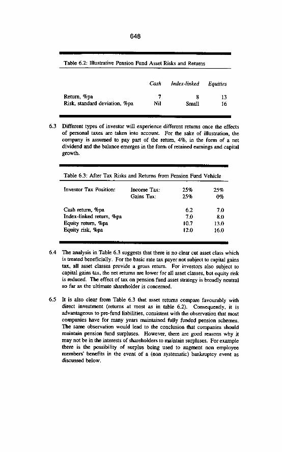
Table 6.2: Illustrative Pension Fund Asset Risks and Returns

Return, %pa Risk, standard deviation, %pa

Cash Index-linked Equities

7 8 13 Nil Small 16

6.3 Different types of investor will experience different returns once the effects of personal taxes are taken into account. For the sake of illustration, the company is assumed to pay part of the return, 4%, in the form of a net dividend and the balance emerges in the form of retained earnings and capital growth.

Table 6.3: After Tax Risks and Returns from Pension Fund Vehicle

Investor Tax Position: Income Tax: Gains Tax:

-

25% 25% 25% 0%

Cash return, %pa 6.2 7.0 Index-linked return, %pa 1.0 8.0 Equity return, Ipa 10.7 13.0 Equity risk, %pa 12.0 16.0

6.4 The analysis in Table 6.3 suggests that there is no clear cut asset class which is treated beneficially. For the basic rate tax payer not subject to capital gains tax, all asset classes provide a gross return. For investors also subject to capital gains tax, the net returns are lower for all asset classes, but equity risk is reduced. The effect of tax on pension fund asset strategy is broadly neutral so far as the ultimate shareholder is concerned.

6.5 It is also clear from Table 6.3 that asset returns compare favourably with direct investment (returns at most as in table 6.2). Consequently, it is advantageous to pre-fund liabilities, consistent with the observation that most companies have for many years maintained fully funded pension schemes. The same observation would lead to the conclusion that companies should maintain pension fund surpluses. However, there are good reasons why it may not be in the interests of shareholders to maintain surpluses. For example there is the possibility of surplus being used to augment non employee members’ benefits in the event of a (non systematic) bankruptcy event as discussed below.

7 7.1

1.2

1.3

1.4

649

Effects of Bankruptcy Risk and MFR Having granted final salary benefit promises, the use of a low risk investment strategy combined with full funding within a pension fund ensures that employers will meet the full cost of providing these benefits. However, if a high risk investment strategy is used, there is a small chance that there will be a windfall gain to shareholders, in the event of corporate bankruptcy accompanied by a pension fund shortfall arising from a fall in asset prices (that is a systematic bankruptcy event). The gain arises if the deficit is not made up from the remaining assets of the company.

The introduction of MFR can result in a cash call on companies at a time of a decline in equity markets, when companies experience difficulty in raising funds, and trigger corporate bankruptcy. It is perhaps stating the obvious that costs associated with such bankruptcy can be very high. Besides direct costs such as redundancy costs and legal and accountancy fees, goodwill value associated with the possibilities for profitable trading in the future can be lost. Also, it must be borne in mind that any additional funding arising from the MFR might be exposed to non systematic bankruptcy risk if future discontinuance surplus accrues to members ahead of shareholders.

In the past, a pension fund shortfall had few adverse consequences (other than the need to make good the shortfall) since companies could make up the amount over a period of many years. Furthermore, companies were generally able to choose the pace of funding (having regard to taxation, bankruptcy and other issues discussed here). The effect of MFR is potentially to dramatically shorten the timescales over which deficits need to be covered and to trigger bankruptcy where a company is unable to access internal or external funds within the period. The effect is lessened if, as currently envisaged, the imposition of MFR is suspended during an extreme market crash. Further, scheme trustees may decide not to insist that the shortfall be made up, in the event that this would lead to bankruptcy.

Part three of this paper develops a model to reflect the implications for investment policy of bankruptcy risk and MFR.

Part III: A New Methodology 1. Introduction 1.1 In this part the additional returns expected from equity investment are

assumed to be offset by additional risk, relative to investment in the portfolio of assets most closely corresponding to the characteristics of the pension liabilities. Equity markets are assumed to follow a normal diffusion (random walk) process combined with a Poisson jump to encapsulate sudden unexpected shocks. Negative jumps lead to a small frequency of corporate insolvencies which in turn lead to transfers of wealth between shareholders and members depending on the funding position of the pension scheme at the time of insolvency. Section 5 determines the optimal asset mix, and Section 6 assesses optimal funding strategy, from a shareholder standpoint, based on

650

the assumption that members do not participate in pension fund surpluses. Section 7 extends the analysis to the case where there is some sharing of favourable investment performance. Sections 8 examines the issues from a members’ and trustees’ viewpoint whilst Section 9 considers the position from both a shareholder and trustee perspective. The Appendix summarises the notation used in the model and sets out certain proofs.

2. Process For The Market Portfolio 2.1 The market portfolio value P, is assumed to follow the stochastic process;

P, = PO exp ([otMO)

where dM = w.df + B.&I + aq; dn is a standard diffusion process and q = N(O,l), with probability Ldr

0, otherwise.

2.2 The process results in total overall market volatility of approximately 17.5% pa, based on the following parameter settings:

0 = 15% pa, 0 = 20% pa, h = 20% pa.

2.3 The diffusion process is intended to reflect ‘normal’ market fluctuations, while the Poisson jump (which occurs on average once in every five years) is intended to represent sudden unexpected changes in the corporate environment, such as the oil shocks in the early 1970’s, the rapid increase in interest rates imposed by the Government in the early 1980’s and again in the late 1980’s (all negative shocks), or the relaxation of credit controls and reductions in taxation in the mid 1980’s, and the exit of the UK from the ill- conceived European exchange rate mechanism in 1992, etc (positive shocks).

3. Mathematical Representation of the Process for Corporate Bankruptcy 3.1 For simplicity we will assume that systematic bankruptcy risk arises only from

the Poisson jump terms in the above process.

3.2 We assume that the value V of a firm follows the following stochastic process, in the absence of pension fund risk (that is, assuming that the pension fund follows a matched strategy):

dV = p.V.( exp( udt + dM ) - 1 ), where

u compensates for systematic bankruptcy risk and j3, represents systematic market risk, that is sensitivity to market returns.

3.3 Bankruptcy of the firm is triggered by the value (V) falling below a ‘floor’ value (V,,,,). That is, if b is bankruptcy risk:

651

b = 1, if dV < V,,, - V and b = 0, otherwise.

If the asset value falls by less than V,,,, - V (that is, the value remains above the floor), then for simplicity we will assume that shareholders can immediately recapitalise the firm back to V. Likewise if the asset value rises above V we assume immediate distribution of the excess to shareholders. This assumption simplifies V to a constant (thereby removing the requirement for our optimal solution to be dependent on this state variable), and is also consistent with systematic bankruptcy risk being triggered only by jump events, since any injections arising from the diffusion process will be of order ddt.

4. Effect of Introducing Pension Fund Mismatch Risk 4.1 We now consider the pension fund, which we initially assume to be. 100%

funded on our market basis. We then assume that this fund follows the process:

dz = s.z.( exp(dM) - 1 ) where z is the initial fund value and s is the allocation to risky assets.

4.2 Again, in order to simplify this model, we assume that the shareholder will recapitalise the fund back to z ‘almost immediately’. However, we make this process rather fuzzy by assuming that only the shortfall below z,,” (some statutory minimum funding level) contributes to the calculation of bankruptcy risk and although the shareholder will return the fund back to z quickly, the flexibility in this process allows him to do so at times when bankruptcy is not a danger (that is, in between shocks).

4.3 Without this final assumption there is need for a dynamic solution. However, by transferring the dynamism to the funding policy we can side step this issue here for the time being (that is, we effectively assume that z is broadly constant just before any jump through dynamic funding, rather than through a riskless investment strategy).

4.4 With this assumption, the condition for bankruptcy becomes:

b = 1, if (dV<: V,,,, - Vand dz > zmin - z). b = I, if (dV + dz + z - z,,, < V,,,,, - V and dz < z,,,, - z],

b = 0, otherwise. 5. Optimal Pension Fund Strategy from a Shareholder Perspective 5.1 We now consider the choice of an optimal strategy from a shareholder’s

perspective, defined as the strategy which minimises his loss on bankruptcy, or equivalently, maximises the amount of pension liabilities on which the firm can default.

652

5.2 This benefit can be extracted by the shareholder if he holds a short position, outside the firm, of s.z in the market portfolio. Applying the ‘look through’ principle, the value of this combined position is -b(dM).s.z.(exp(&f) - l), a non negative quantity that is monotonic in s (it is zero if no bankruptcy occurs).

5.3 The pension fund mismatch will not increase the risk of the firm (and therefore corporate bankruptcy results in a risk free gain to the shareholder at the expense of scheme members), unless the overall risk of bankruptcy is increased as a consequence of the requirement to fund shortfalls below z,,,,“.

5.4 Now, in the absence of pension fund risk (SO), if bankruptcy occurs for a poisson jump of q’ (or less) then:

q’ = (l/cr).log(l+(v,,-v~/@.v),

It is trivial to show (see Appendix A) that this risk of bankruptcy is not increased by the addition of pension fund risk provided that we choose s to ensure that:

q’ > (l/0).log(l+(z,,-z)Io).

Hence, assuming that the utility placed on loss arising from an increase in overall bankruptcy risk of the firm always exceeds the marginal advantage from further default on pension liabilities, the optimal strategy S* satisfies:

s* = I(z-z,,.)~zl.fP. wv-v,,,)1

5.5 Under this simple model it is optimal for the shareholder to choose s’ so as to ensure that the pension fund assets fall below z,,,, coincident with the firm value (excluding pension fund) falling below Vnh and triggering corporate insolvency, (the loss of value resulting from the latter event is assumed to be very large). This can be verified intuitively since, if the firm goes bankrupt when q = q’ with z still above zminr the firm has been unnecessarily cautious in its choice of s, which can be increased without increasing bankruptcy risk. On the other hand, if z is below z* when q = q’ then the trigger point for bankruptcy is above q’ and bankruptcy risk can be reduced by reducing S.

5.6 To illustrate this, consider a systematic bankruptcy risk of 0.1 %pa for a large firm, 0.5% pa for a medium sized firm, both with beta of one, and 1.5% p.a. for a small firm with a beta of two. The following table shows the implied bankruptcy floors and optimal strategies, assuming a z,~, value of 75% of the final salary liabilities:

653

Table 5.6: Expected bankruptcy gain for large, medium and small firm.

Large Medium StPUlll

Systematic bankruptcy risk Beta Implied bankruptcy floor Optimal equity allocation Expected gain (% pension liabilities)

0.1% pa 1.0

60.0% 62.5%

0.03% pa

0.5% pa 1.0

67.6% 77.2%

0.16% pa

1.5% pa 2.0

50.0% 100.0%

0.50% pa

5.7

5.8

5.9

In the table, the expected gain (G) is calculated as:

~[GJ=ls*.z.~Jl -exp(oq)).&dq

where ‘$ is the normal density function.

In practice, the expected gains arise when markets have fallen sharply and therefore provide significant diversification benefits. The expected utility of the gain is therefore likely to be high for most investors.

These results may appear strange or counter intuitive at first sight. However, from a shareholders perspective they are quite rational. A shareholder investing in the small firm is exposed to significant bankruptcy risk even in the absence of pension fund risk, since (by contrast with the larger firm) the firm will go bankrupt for relatively small jumps. It is therefore not worthwhile for him to insure. the pension fund (at a level above z,,,,) for very extreme jumps, since the firm will already be bankrupt. On the other hand, a shareholder in a larger firm has a different perspective. He expects the firm to go bankrupt only under very extreme market movements and it is therefore important that the pension fund does not fall below zmin under less extreme systematic events, since this would serve to increase bankruptcy risk.

The result can also be verified in the limit as bankruptcy risk declines to nil. For such a firm, current and deferred pension obligations are equivalent to the issue of very secure bonds. Absent any opportunity to default (and ignoring any tax advantages), there is no reason, using this model, for shareholders to prefer equities over government bonds.

The model also appears realistic in a more general dynamic setting. For example, if a shock occurred and the bankruptcy risk of a firm increased, the shareholder would allow the risk of pension shortfall to increase. The shareholder would become more ‘fatalistic’. As a consequence the optimal equity allocation may not be perturbed. By contrast, if the shareholder became less risk tolerant (or risk tolerance remained constant) as bankruptcy

654

risk increased, the shock would trigger a reduction in equity exposure and a potential portfolio insurance spiral. This ‘system stability’ supports the idea that the equation is the ‘right way round despite at first sight being counter intuitive.

5.10 The result has interesting implications for the valuation of pension scheme liabilities from the shareholder’s perspective, where the margin in the discount rate to reflect the benefits of equity investment should be a function of the expected gains shown above (it would be appropriate to weight these gains to reflect the fact that the payout occurs in times of distress). Accordingly the results in the table suggest using higher discount rates to value the liabilities of smaller, less secure, firms. This seems intuitively correct. In the limiting case of a Government backed scheme, index linked pension liabilities would be valued identically with equivalent index linked gilts (although, other implicit margins may need to be included in the real salary and withdrawal assumptions for active liabilities). The conclusion does, however, conflict with the basis proposed for MFR, which is weaker for larger schemes.

6. 6.1

6.2

6.3

Optimal Funding Policy So far we have assumed that the liabilities are 100% funded (say z = z,,.J. However, our analysis suggests that the optimal level of equity investment (and the bankruptcy gain from this) increases as the ratio of the fund (z) to minimum liabilities (z,,,) increases. In this and the following section we analyse whether it is possible to establish an optimal investment and funding policy to maximise bankruptcy gain.

Consider the injection of an additional amount (z - z,,.J, which is lost on bankruptcy, and the associated ‘bankruptcy gain’ from this policy. If a Poisson jump occurs, for any 4 < q’, this gain G(z) is;

G Czl = (2,&J - z) + z.s’. (I - exp (aq)),

it is zero otherwise.

It is trivial to show (see Appendix A) that for q < q*, this is a monotonically increasing function of z, so we are again in the position (from a shareholders’ perspective) of simply adopting the highest funding policy possible. It should be noted here that the benefits are assumed fixed so that there is no leakage towards increased benefit levels in the event of favourable investment performance. This aspect is considered in Section 7, as are other reasons why lower funding may be appropriate.

In the absence of other practical (eg taxation) constraints, this policy of maximising the funding level is constrained only by the associated optimal s*, which will increase also without limit. Although such leveraged solutions are valid from a shareholder’s perspective, they involve the pension fund adopting an increasingly geared equity exposure and the firm defaulting not only on pension liabilities but on the fund’s borrowings. It is unlikely that any counter party would accept this without some premium. Accordingly we

655

regard the optimal funding level (2’) (ignoring taxation effects) as the policy which yields a 100% exposure to risky assets, that is

z I- - Gn,, / (1 - w-v,,,)4Pv))

6.4 However, this would generally result in a funding level well in excess of those observed in the UK (for example, for our large firm it suggest an optimal funding level of 167%). In the next section we complete our analysis of the shareholders’s optimal policy, by investigating reasons why lower funding may be optimal.

7. Leakage 7.1 Distribution of surplus to scheme members (through benefit improvements or

members’ contribution reductions) represents ‘leakage’ of gains from a shareholder’s perspective. Furthermore, a second leakage effect arises if a firm increases the funding level through an increase in contributions. Shareholders are then worse off in the event that the firm subsequently goes into bankruptcy and there is a pension fund surplus which cannot be recovered. Such losses arising as a result of non-systematic bankruptcy risk, not included in the model, would lead to leakage and a reduction in optimal funding. For the sake of brevity these non systematic effects are not considered further in this paper, although they can be modelled approximately by applying a constant (generally small) force of discount to the shareholders’ pay off from the fund.

7.2 Instead, we will simply assume that scheme members do participate (immediately) in a proportion t+r of any surplus above a threshold funding level a-. The loss to the shareholder is:

L(z) = y.[sz.(exp (09) - 1) - fz,, - z)l

for q > (I/a). log (l+(z,, - z)/(sz)) = q**

(Under our model this is felt immediately by the shareholder as an uncovered short position outside the fund).

7.3 In general, as suggested in part two, member participation in surplus will take the form of discretionary increases (possibly backdated) to pensions already in payment (the cost of such increases, since the increased amount will also be paid in future years, being capitalised as an annuity value). Hence, r+r may be a function of a conventional measure of maturity, such as the overall proportion of pensioner liabilities. In addition, the rate at which the firm can extract surplus may be constrained by the maximum rate of a full contribution holiday. Although not easily incorporated explicitly into this simple model, such a constraint would also tend to have the effect of reducing z,,, in schemes where the new accrual of benefits is small in relation to total liabilities (another common, ‘cashflow’, measure of maturity).

7.4 We have been fortunate so far in deriving optimal policies using only the principle that the shareholder prefers more to less (apart from our reasonable

656

assumption that it is never worthwhile to increase the bankruptcy risk of the firm). However, this leakage effect requires us to trade-off the utility of loss for some q events against the profit in other q events. In order to proceed further we introduce, for illustration purposes only, a simple utility function, u (x,q), dependent on the state of the world q:

u f&q) = xifqc0 = o.xifq>O

7.5 With this simple utility function we now seek the optimal funding policy to maximise:

E W(z)1 = h 1’1 G(z) $ dq - h.w /;,.(1 L(z) 4 4

Since it is crucial to the mathematics which follows, we emphasise that the upper limit of the first integral, q’ is a constant, while the lower limit of the second q” is a function of s. Differentiating this with respect to s is slightly more complex than it may appear at first sight.

7.6 Figures 2a, 2b and 2c below show the values of E[U(z)] and associated s* (z), for a range of values of z, for our large, medium and small firms using the following parameter settings:

Glax = 150 0 = 0.25 v = 0.50

Figure la Expected Utility and Optimal Equity Allocation : Large Firm

657

Figure lb Expected Utility and Optimal Equity Allocation : Medium Firm

Figure lc Expected Utility and Optimal Equity Allocation : Small Firm

7.7 It may appear surprising that (subject to the possibility of weighting more heavily the pay offs in adverse conditions) the overall benefit from equity investment with both an optimal investment policy and funding policy is so small for our large firm (the maximum being of the order of 3 basis points per annum). However, it should be noted that this applies to a ‘large’ firm with a systematic bankruptcy risk of only 0.1% pa. In other words, investing in the debt of such ‘blue chip’ firms is almost the same as investing in government bonds (apart from liquidity considerations). Accordingly, it should not be surprising that from a purely financial perspective the benefit from equity investment is marginal. What is more important in this context is that there is some marginal benefit and this is additional to the other factors discussed in Part II (not quantified here) which also serve to support such investment. The benefit is of a much greater order of magnitude (of order 50 basis points per annum) for our small firm.

658

8. Optimal Strategy from a Trustee Perspective 8.1 Finally we consider optimal strategy from the opposite perspective, that of the

trustee.

8.2 If we make the assumptions that:

(1) leverage (that is, borrowing is again disallowed, (2) it is not in the members’ interests to increase the bankruptcy risk of the

firm (this would be a questionable assumption for a closed fund comprising mainly pensioners and deferred pensioners with no direct interest in the survival of the firm),

(3) the utility placed on payouts during positive or negative jumps is broadly the same as that of the shareholder (ie more benefit is derived from a positive payout in adverse states of the world than in benign states), and

(4) the members benefit fully from any surplus funds in the event that the pension scheme is wound up on corporate bankruptcy,

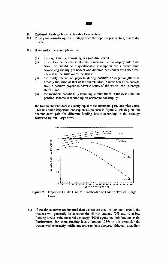
the loss to shareholders is exactly equal to the members’ gain, and vice versa. This has some important consequences, as seen in figure 2, which plots the shareholders’ gain for different funding levels according to the strategy followed by our large firm.

Figure 2 Expected Utility Gain to Shareholder or Loss to Trustee: Large Firm

8.3 If the above curves are inverted then we can see that the maximum gain to the trustees will generally lie at either the nil risk strategy (0% equity) at low funding levels or the most risky strategy (100% equity) at high funding levels. Furthermore, for some funding levels (around 123% in this example) the trustee will be broadly indifferent between these choices, (although, a medium

659

risk strategy will represent the worst of all worlds!) For the medium firm this point of indifference between the nil and high equity strategies (but aversion to intermediate risk) is attained at a much higher funding level (148%). For the small firm the preference is for low risk strategies at all funding levels.

9. The Balance between Shareholders and Trustees 9.1 In the absence of mutual ‘insurance’ synergies (which would occur, for

example, if trustees placed more utility weight on surplus participation than bankruptcy loss, while shareholders held opposite preferences), the above model essentially describes a zero-sum-game between shareholders and trustees. Whilst such insurance effects cannot be dismissed entirely (for example, if trustees place more emphasis on the interests of current pensioners, and give them priority on scheme assets ahead of active and deferred members), investment policy under this model generally acts merely as a mechanism for transferring benefit between shareholders and scheme members in different scenarios, with one party gaining only at the expense of the other. The only exception to this rule is at low ‘solvency’ levels, where both parties are assumed to be averse to any increase in the overall bankruptcy risk, so that both parties agree on a low risk approach.

9.2 This construction makes for a rather adversarial conflict between the two interested parties, (that is, shareholders do not necessarily always prefer the more risky approach, nor do trustees necessarily prefer the more prudent strategy).

9.3 This is not an encouraging result for those seeking a consensus between trustees and shareholders. However, it would appear unreasonable to expect any model to suggest that a firm can rearrange its assets not only to increase shareholder value but also to increase the value of obligations given to creditors (whether corporate bond holders or pension scheme members)! Accordingly, the conclusion again appears intuitively correct.

9.4 In this context it is therefore interesting to ask not only why high equity strategies might be optimal for some funds (which we have now addressed) but why such high equity strategies are adopted almost universally, apparently regardless of maturity (‘leakage’), level of funding or size of firm. If we assume that this represents rational behaviour then this could be explained by variations in the dominance of shareholder versus trustee (or other ‘stakeholder’) interests according to firm size.

9.5 For example, if we consider a large firm (low bankruptcy risk) with a mature fund (high leakage) then it is likely to be in the trustees interests to pursue a high risk strategy and in the shareholder’s interest to follow a low risk strategy. Furthermore, if the non-employee membership is high, it may even be worthwhile for the trustees to pursue a strategy which increases the overall bankruptcy risk of the firm. Accordingly, a high equity strategy in this example would be indicative of trustee interests dominating, which may not be an unreasonable conclusion for some large institutional&d firms.

660

9.6 At the opposite extreme, if we consider a small firm (high bankruptcy risk) with an immature fund (low leakage) then it is likely to be in shareholders interests to pursue a high equity strategy, provided that the solvency level is sufficient to support this without increasing overall bankruptcy risk. Accordingly a high equity allocation would be indicative of shareholder dominance. Again this may not be unreasonable in such a firm, where there is likely to be a more ‘active’ influence from shareholders.

9.7 In this context, the equity backed element of the UK minimum funding basis, may prove to be something of a double edged sword. Certainly, this should have the effect of significantly weakening the standard in times of corporate distress, the concession for large schemes weakening the basis more for larger firms. However, by supporting equity investment (indeed creating an artificial risk of not investing in equities) the choice of basis may act in the interests of trustees rather than shareholders of large firms.

Part IV: Conclusions The principal conclusions emerging from the analyses contained in the first part of this paper are:

. The suggestion that equity risk declines with time horizon is of very doubtful validity (1.2).

. The additional return expected from investing in equities is offset by extra risk, so that equities are not a superior asset simply because of their higher expected return (1.3).

. The use of actuarial discounted cash flow values rather than market values will render conclusions from traditional asset/liability studies invalid (1.4).

. Asset/liability analysis should by dynamic. The more usual state framework, can result in a misspeciftcation true risks.

Part two of this paper:

. Sets out an economic rationale for the provision of final salary related benefits (11.1) and for the use of a separate funding vehicle (11.2).

n Highlights three broadly equivalent ways a shareholder can gain equity exposure, directly held assets, gearing of the balance sheet or through pension fund strategy (11.3).

. Argues that a matching strategy, including substantial investment in index linked and conventional gilts provides significant benefits (11.4), although there are a number of reasons why investment in other asset classes, may also be optimal (11.5).

661

. Shows that the effect of a corporate insolvency, combined with a high risk investment strategy, may be to provide a windfall gain to shareholders in the event that there is a pension fund shortfall (11.6). However, that the resulting preference for equity investment reduces upon the introduction of MFR. since cash calls at a time of a decline in equity markets could trigger bankruptcy, and additional funding may be lost on company specific bankruptcy events (11.7).

The mathematical models developed in part three of the paper show that:

The bankruptcy and MFR effects noted in II.6 and II.7 result in an optimal level of equity investment (111.5) and an optimal funding policy (III.6).

This optimal policy is significantly modified if members participate in surpluses (III.7).

From a trustee perspective, optimal strategy is nil risk (100% matching) if companies follow a low funding policy and have high bankruptcy risk, or high risk (100% equity) for strongly funded schemes of creditworthy companies (111.8)

There is some conflict between the interests of shareholders and members except, post MFR. where a pension fund shortfall could lead to corporate bankruptcy (111.9).

We consider that the arguments presented in support of adopting an asset strategy broadly matching the liability payments are very powerful from a shareholder’s perspective. This would not preclude some element of equity investment.

The bankruptcy and leakage effects suggest that there are some benefits to departure from a matching strategy to trustees or to shareholders (but not both).

The results also have significant implications for pension fund valuation methods and assumptions which merit further consideration.

References

Barclays de Zoete Wedd (1995). Equity gilts study. Black, F & &holes, M (1973). The pricing of options and corporate liabilities. Journal of Political Economy, 81, 637-654. Bodie, Z (1995). On the risk of stocks in the long run. Financial Analysts Journal, May/June 18-22. Clark, G (1992). Asset and liability modelling - the way ahead. Staple Inn Actuarial Society. Exley, CJ, Mehta, SJB and Smith AD (1996). Market efficiency. 1996 Investment Conference. Goetzmann, WN & Jorion, P (1993). Testing the predictive power of dividend yields. The Journal of Finance, Vol XIV111 No 2. Goetzmann, WN & Jorion, P (1993). A longer look at dividend yields. Journal of

662

Business, Vol 68 No 4. Ibbotson, RG & Sinquefield, RA (1989). Stocks, bonds, bills and inflation: historical returns (1926-1987). The Research Foundation of the Institute of Chartered Financial Analysts, Charlottesville, Virginia. Leland (1994). Corporate debt value, bond covenants and optimal capital structure. Journal of Finance, 1213-1252. Lockyer, PR (1990). Further applications of stochastic investment models. Staple Inn Actuarial Society. Merton, RC & Samuelson, P (1974). Fallacy of the log-normal approximation to optimal portfolio decision-making over many periods. Journal of Financial Economics 1, 67-94, North Holland. Modigliani, F & Miller, MH (1958). The cost of capital, corporation finance and the theory of investment. American Economic Review, 48: 261-297. Nelson, CR & Kim, MJ (1993). Predictable stock returns. The Role of Small Sample Bias. The Journal of finance Vol VIII, No 2. Redington, FM (1952). Review of the principles of life office valuation, JIA 78, 286-315. Samuelson, P (1969). Lifetime portfolio selection by dynamic stochastic programming. The Review of Economics and Statistics LI, 239-246. Sherris, M (1992). Portfolio Selection and Matching: a synthesis. JIA 119, 87- 105. Smith, AD (1996). How actuaries can use financial economics. BAJ. Thorley, SR (1995). The Time-Diversification Controversy. Financial Analysts Journal. Thornton, PN & Wilson, AF (1992). A realistic approach to pension funding. JIA 119, 229-312. Wilkie, AD (1995). More on a stochastic asset model for actuarial use. BAJ 1, 777-964.

663

APPENDIX

1 Some terminology

V Value of a firm (excludes pension assets and liabilities), dV=PV(exp (udt + dM)-1) M dM

2 S

Zmin S*

q*

G

Z* 0 v L

I* q

Fundamental factors driving the market portfolio P = wdt + 9dn + oq, with probability Mt, q is N(O,l) = wdt + Odn, otherwise, where dn is a standard diffusion process Company beta ratio Compensates investors for systematic bankruptcy risk = 1 if dV <Vmin - V, bankruptcy arises if firm value declines below a floor Vmin = 0 otherwise (see also 111.4.4) Fund, dz=sz (exp (dM) -1) Allocation to risky assets Statutory minimum funding level p (Z - Zmin)V/(zK), optimal allocation to risky assets, k = V-Vmin Poisson jump above which bankruptcy risk is not increased by non discretionary additional contributions Annual gain to shareholders, being pension liabilities not paid on corporate bankruptcy, proportion of liabilities Optimal funding level weight placed on payout for q>o member participation in surplus for z> z,, Annual leakage to members arising from benefit increases (less to shareholders) Poisson jump above which leakage occur

664

2 Maximum s(z) for which bankruptcy risk is minimised

We will apply repeatedly the simple algebraic result that for c&O, if b/d >(a+b)l(c+d),

then (a+b)/(c+d) > a/c

If we define the set Q as

Q = (q : b(dm) = l),

then, for s > (z-z&/z we have:

Q = (4 : ql < q < e) U 1 9 : q < min (qdbll

where:

91 =

42 =

9 3 = and

l/O log [l + (z’-z)/(sz)];

l/a log [l + (V’-V)/@V)];

l/a log [l + (V’-V+Z’-z)/@v+sz)];

Q = (q : q < qr) otherwise

First note that, if s < (z - z,,)/z, then supQ = e (constant)

Also, q,, and qr are both monotonic increasing functions of s if =ztin and k-v,,.

Our objective is then to find the maximum s such that sup Q = 92. Now, if q, > e then by our simple algebraic result q, > e, and so:

Q = (q : q < ~1, where q3 > e

By similar reasoning, if q, < q, then:

Q = (4 : q < ~1, where q, > q3 > q1

It follows that the desired maximum S* satisfies:

q, = e = q,, or:

(z,,-ZMSZ) = cv,.-vYcP

3 Bankruptcy gain G(z) is a monotonic increasing function of z

We wish to prove that for all q < q’,

G (2) = z.s(z).((l-exp(oq))) - z

is an increasing function of z, where

s(z) = [(z-z’)/z] [pv/(v-V’)]

and q’ = (I/a) log [ 1 + (V’-V)@V)]

Taking the derivative with respect to z:

G’ (z) = [s(z) + zs’ (z)] (I-exp(oq)) - 1

= [(z-z’)/z pV/(V-V’) + (z-/z) pV/(V-V*)] (1-exp(oq)) -1

= [pV/(V-V’)] (1-exp(oq)) - 1 > 0 if q<q’.