associate professor mariano gonzÁlez sÁnchez, … - mariano g. sanchez,(t).pdfequilibrium exchange...
TRANSCRIPT

Associate Professor Mariano GONZÁLEZ SÁNCHEZ, PhD
Email: [email protected]
Business and Economics Department. CEU Cardenal Herrera University
Professor Juan M. NAVE PINEDA, PhD
Email: [email protected]
Finance and Economic Analysis Department
Castilla La Mancha University
COMMON STOCHASTIC TRENDS AND EFFICIENCY IN THE
FOREIGN EXCHANGE MARKET
Abstract. Within the traditional financial literature about efficient markets there
are two interpretations on empirical results, some works find evidence of the
predictive superiority of the martingale (martingale hypothesis); while others provide
evidence supporting a hypothesis of cointegration among exchange rates. In this
context, we analyze triangular arbitrage cointegration relationship, among Dollar-US,
Euro and others 20 currencies, to test efficiency market of exchange rates. For this, we
consider implicit transaction costs in daily Ask-Bid cointegration relationships with
heteroskedasticity covariance matrix, and using alternative methods: cointegration
relations with and without heteroskedasticity, and dynamic factorial analysis. We do
not find empirical evidence of the lack of arbitrage opportunities, so the results
support efficiency of the exchange markets.
Key words: efficient market, cointegration, opportunities arbitrage, transaction
cost, BEKK.
JEL Classification: C32, F31, G14.
1. Introduction
As world trade needs to know what the equilibrium exchange rates in the long
term, with the disadvantage that fluctuations in the short-term market exchange rate
could not be full explained by macro variables, in the financial literature arise works
on the foreign exchange market efficiency. This question has been studied from three
perspectives.
This work was supported by the research project of the Spanish Government (MEYC ECO 2012-36685) and
Generalitat Valenciana (PROMETEO-II/2013/015).

Mariano Gonzalez , Juan Nave
First, to study when exchange rates have been in a state of equilibrium respect
interest rates and price levels. These works estimate a time-varying behavioural
equilibrium exchange rate testing differences theories as Purchasing Power Parity
(PPP), Covered Interest Parity (CIP), Expectations Theory (ET), Uncovered Interest
Parity (UIP) and Fisher Effect (FE) hypothesis (among others: Caporale et al., 2001). Second, to research if the forward exchange rate is an unbiased predictor of
future spot exchange rates, i.e., forward rate unbiasedness hypothesis (see: Baillie and
Bollerslev, 1989).
Third, our study matter, to test the spot exchange market efficiency (see:
Diebold et al., 1994; Crowder, 1994). For this goal, the empirical works use
cointegration techniques to analysis the triangular arbitrage relation. The results have
two possible interpretations:
— If there is not cointegration relationship, the foreign exchange market is
efficient, that is, changes in exchange rates are unpredictable. In other
words, if one could forecast a exchange rate on the basis of other one in the
cointegrated system, then hypothesis martingale would be violated (Diebold
et al., 1994).
— Efficiency and cointegration are not opposite, as argue Crowder (1994),
among others. Thus, a market is efficient when there are no risk-free returns
above opportunity cost.
The initial empirical studies on triangular arbitrage used monthly or weekly
data. Dutt and Ghosh (1999) for weekly data from the New York Money Market and
International Financial Statistics Monthly, from January 1973 to April-1994, rejected
that markets are efficient. Since the market operations are becoming increasingly
automated, the most recent studies analyze daily or high frequency data.
In this context, Martens and Kofman (1998), contrasting data from the Reuters
platform FXFX high frequency (1-3 minutes) with the currency forward prices on the
Chicago Mercantile Exchange, found apparent arbitrage opportunities against the
forward-spot price Reuters, concluding that the use of different data sources could lead
to conflicting results. Kollias and Metaxas (2001) used data tick to tick, concluding
that arbitrage opportunities have very short duration and, cannot be regarded as market
inefficiencies, but to an effect of slippages of currency market quotes. Marshall and
Treepongkaruna (2008), with high frequency data (less than 5 minutes) from the EBS
platform, found evidence of small triangular arbitrage opportunities, which increasing
the observation time of the data disappear. Fong et al. (2008) found evidence of
arbitrage opportunities in high frequency data for spot and forward exchange rate of
US-Dollar and Hong Kong- Dollar, but they noted that the theoretical benefits occur in
low market liquidity and likely, transaction costs would offset it mostly. Fenn et al.
(2009) found arbitrage opportunities in the spot market exchange rate by triangular
arbitrage operations in high-frequency observations obtained by Reuters to refresh 5
Common Stochastic Trends and Efficiency in the Foreign Exchange Market
minutes, concluding that the market is not efficient, but these opportunities are more
than 94% of cases of a magnitude less than 1 b.p. (basic point) and with a duration of
less than 1 second, further such opportunities are manifested in extreme hours from
GMT (Greenwich Mean Time). Moore and Payne (2011) show that the volume of the
operation and size of the operator are two significant variables of arbitrage
opportunities, and in the case of cross-exchange market, they find that the cross-traders
are the group operators with better information, so one might conclude that the
arbitrage opportunities, if any, are limited by the size and time. Kozhan and Tham
(2012), found evidence of triangular arbitrage opportunities are not exploited
immediately, so they conclude those either are not optimal either not financially
compensate the operators. Chung and Hrazdil (2012) show that price adjustments to
new information do not occur instantly.
Additionally, for high frequency data arise the synchronization problem among
the prices of different financial assets. Akram et al. (2008) found evidence of arbitrage
opportunities in high frequency data, but to solve the problem of synchronization,
chose to work with the last price offered in each case (stale quotes), without
considering further that to close an operation in a market, operators require a minimum
time. Gagnon and Karolyi (2010) show that using illiquidity and stale quotes could
lead to erroneous conclusions because of the intrinsic problems of the original data,
resulting in spurious arbitrage opportunities.
Besides above problems, as the literature has progressed, it has moved from
considering only price bid, to analyze the prices adjusted to the reality of trading in the
foreign exchange market. As we know the market-makers must give orders to ask and
bid prices simultaneously (two-way or round-trip quotes1). However, the
methodological approach of many papers does not analyze jointly the behavior of both
prices, operating with the spread or both prices separately. For example Fenn et al.
(2009) estimated separately ask and bid price and then, compare theses prices to
contrast arbitrage opportunities, so they obviate the multivariate distribution of the 6
variables (2 prices, ask-bid for 3 currencies). Others, as Choi (2011), uses a theoretical
average spread, resulting from the observed spread and unobserved weighting, also left
aside the long-term relationship or equilibrium among the exchange rate variables (not
stationary), since operates with relative variation rates (stationary).
In summary, we observe recurrent problems in the studies about arbitrage
opportunities on high frequency data: the minimum margin, the short duration, in
extreme hours from GMT, the low liquidity for potential arbitrage opportunities, the
stale quotes and the failure to consider the bid-ask spread.
1 Round-trip and one-way arbitrage conditions differ in that violations of the latter do not necessarily prove the
existence of riskless profits, so one-way requires an excess supply or demand of fund, while round-trip not. As consequence, one-way arbitrage opportunities only indicate quote differentials that are due to different practices and
market segmentation
Mariano Gonzalez , Juan Nave
Therefore, the aim of this paper is to study if cointegration and efficiency are
possible simultaneously in foreign exchange market, or if there are arbitrage
opportunities. For that, we identify the structure of Vector Error Correction Model
(VECM) of triangular arbitrage among 20 daily spot prices against Dollar-USA (USD)
and Euro (EUR) from a single platform (Reuters), thus avoiding the problems
synchronization, and using Ask and Bid exchange rate, this allows to reply more
exactly hedged portfolio and to include the implicit transaction costs.
The remainder of this paper is organised as follows. Section 2 reviews the
financial relations of the model. Section 3 shows the econometric methodology used.
In Section 4 we present the data. The results are in Section 5. Finally, the conclusions
are in Section 6.
2. The Triangular Arbitrage
The cross exchange or triangular arbitrage is defined as:
(𝐶𝑖
𝐶𝑗)
𝑡
≡ (𝐶𝑖
𝐶ℎ)
𝑡× (
𝐶ℎ
𝐶𝑗)
𝑡
(1)
Where (Ci, Cj, Ch) are three currencies for a day t and its three possible spot
exchange rates are expressed as a ratio.
So, if we operate with three currencies and their respective bid and ask prices,
there are six triangular relations among them: three relationships of ask type and other
three bid type. Among them, two are usually studied in isolation from the rest:
Forward Arbitrage (bid = ask x ask) and Reverse Arbitrage (ask = bid x bid).
In a frictionless market, taking logarithms in (1) to obtain a linear triangular
arbitrage relationship, results:
𝑙𝑛 [(𝐶𝑖
𝐶𝑗)
𝑡
] = 𝑙𝑛 [(𝐶𝑖
𝐶ℎ)
𝑡] + 𝑙𝑛 [(
𝐶ℎ
𝐶𝑗)
𝑡
] (2)
When we consider frictions, then implicit transaction costs suppose that there
are two simultaneous exchange rates (Ask and Bid prices) and the relation (2) is:
𝑙𝑛 [(𝐶𝑖
𝐶𝑗)
𝑡,𝜓
] = 𝑙𝑛 [(𝐶𝑖
𝐶ℎ)
𝑡,𝜓] + 𝑙𝑛 [(
𝐶ℎ
𝐶𝑗)
𝑡,𝜓
] 𝜓 = 𝑎, 𝑏 (3)
Where a is Ask price and b Bid price.
In order to obtain triangular arbitrage relations considering both market sides
(offer and demand), we include the implicit transaction cost rate (𝜇𝑖,𝑗). So, implicit
transaction cost is: 𝑒𝑥𝑝 [(𝐶𝑖 𝐶𝑗⁄ )
𝑡,𝑏
(𝐶𝑖 𝐶𝑗⁄ )𝑡,𝑎
].
Then, we express the Ask-Bid relation between two currencies as follow:
Common Stochastic Trends and Efficiency in the Foreign Exchange Market
𝑙𝑛 [(𝐶𝑖
𝐶𝑗)
𝑡,𝑏
] = 𝜇𝑖,𝑗,𝑡 + 𝑙𝑛 [(𝐶𝑖
𝐶𝑗)
𝑡,𝑎
] (4)
The expected value of transaction cost rate is (𝜇𝑖,𝑗 > 0), because dealers buy
cheap and sell expensive.
3. Econometric Methodology
As our aim is testing exchange rate market efficiency, we contrast if there are
arbitrage opportunities in the long-run triangular arbitrage relation. For this, the
general expression for arbitrage strategies (3) becomes the following econometric
model:
𝑙𝑛 [(
𝐶𝑖
𝐶𝑗)
𝑡,𝜓
] = 𝛿𝑖,𝑗𝜓
+ 𝜆𝑖,ℎ𝜓
𝑙𝑛 [(𝐶𝑖
𝐶ℎ)
𝑡,𝜓] + 𝜆ℎ,𝑗
𝜓𝑙𝑛 [(
𝐶ℎ
𝐶𝑗)
𝑡,𝜓
] + 𝑢𝑖,𝑗,𝑡𝜓
𝑢𝑖,𝑗,𝑡𝜓
~𝑖𝑖𝑑(0, 𝜛𝑖,𝑗2 ) ∀𝑖 ≠ 𝑗 ≠ ℎ 𝜓 = 𝑎, 𝑏
(5)
Where 𝛿𝑖,𝑗𝜓
is the long-run result of triangular arbitrage for currency i with 𝜓
price. The parameters 𝜆𝑖,ℎ𝜓
and 𝜆ℎ,𝑗𝜓
are the weights in reply portfolio of currencies h
and j, respectively and, its expected value according to (3) is |𝜆∗,ℎ𝜓
| = 1.
In the same way, Ask-Bid relation (4) becomes:
𝑙𝑛 [(𝐶𝑖
𝐶𝑗)
𝑡,𝑏
] = 𝜇𝑖,𝑗 + 𝑖,𝑗
𝑙𝑛 [(𝐶𝑖
𝐶ℎ)
𝑡,𝑎] + 𝑖,𝑗,𝑡 𝑖,𝑗,𝑡~𝑖𝑖𝑑(0, 𝜎𝑖,𝑗
2 ) (6)
Where expected value according to (4) is𝑖,𝑗
= 1.
In presence of transaction cost, we have Bid and Ask prices at the same time,
and if we trade on both sides of the market, as occur in the trading arbitrage strategies,
the no arbitrage condition with transaction costs implies: 𝜇𝑖,𝑗 > 0, 𝛿𝑖,𝑗𝜓
≠ 0 and
𝜇𝑖,𝑗 − 𝛿𝑖,𝑗𝜓
= 0. That is, if there are not arbitrages opportunities, the transaction costs of
both sides would be netting.
In this context, the no arbitrage condition implies the existence of a
cointegration relationship among exchange rate of (Ci, Cj, Ch) currencies. To verify
this it is sufficient to analyze the relationship among the error terms of (5) and (6):
𝑖,𝑗,𝑡 = −𝑢𝑖,ℎ,𝑡𝑎 + 𝑢ℎ,𝑗,𝑡
𝑏 = 𝑢𝑖,ℎ,𝑡𝑏 − 𝑢ℎ,𝑗,𝑡
𝑎
𝑖,ℎ,𝑡 = −(𝑢𝑖,𝑗,𝑡𝑎 + 𝑢ℎ,𝑗,𝑡
𝑎 ) = 𝑢𝑖,𝑗,𝑡𝑏 + 𝑢ℎ,𝑗,𝑡
𝑏
ℎ,𝑗,𝑡 = −(𝑢𝑖,𝑗,𝑡𝑎 + 𝑢𝑖,ℎ,𝑡
𝑎 ) = 𝑢𝑖,𝑗,𝑡𝑏 + 𝑢𝑖,ℎ,𝑡
𝑏
(7)
Mariano Gonzalez , Juan Nave
In practice, this result is employed to test market efficiency. For so doing, we
express the problem of efficiency in VECM form as:
∆𝑡 = · 𝑡−1 + ∑ 𝛿𝑑 · ∆𝑡−𝑑𝑘𝑑=1 + 𝑡 (8)
Where X is a vector (with dimension: 6 rows and 1 column) of the logarithms
exchange rate Ask and Bid for three currencies (Ci, Cj, Ch). (∆) is the first difference
operator, and () is a matrix whose rank (r) indicates the number of cointegration
relationship. The decomposition of the matrix is: = 𝛼 · 𝛽′, where 𝛼 is the
adjustment coefficients matrix and 𝛽 is the coefficient matrix of the cointegration
relationship.
The interpretations of k and r in (8) are the usual in cointegration context:
— If k=1 and r=0 then, the exchange rate is a pure martingale.
— If k>1 and r=0 then, the exchange rate has a dynamic behaviour.
— If k>1 and r>0 then, there are (r) stationary relations and the process is long
memory. For this case, we study if efficiency and cointegration are opposite or not.
The expression (8) could be estimated by applying the methodology of Johansen
(1988) and using AIC (Akaike Information Criterion) and SIC (Schwartz Information
Criterion) to select the optimal lags (k).
Cheung and Lai (1993) showed that robustness of Johansen´s LR tests (log-
likelihood ratio) depends on a suitable selection of lags, and when data is moving-
average, the information criterions perform poorly in selecting the optimal lag.
Additionally, Johansen’s LR test assumes homoskedasticity innovations, but the
stylized facts of high frequency financial data in exchange rate (Bos et al., 2000) show
non-Gaussian innovations and heteroskedasticity. For these cases, Cavaliere et al.
(2010), from the previous work of Swensen (2006), propose a pseudo-LR test that,
using wild bootstrap technique, allows contrasting cointegration rank for a VAR-
MGARCH process.
As mentioned above, we expect to find two cointegration relationships (forward
and reverse) among each set of six exchange rates, then we define the next VAR(k)-
BEKK GARCH(1,1) to guarantee that variance is always positive definite:

Common Stochastic Trends and Efficiency in the Foreign Exchange Market
∆𝑡 = · 𝑡−1 + ∑ 𝛿𝑑 · ∆𝑡−𝑑𝑘𝑑=1 + 𝑡 =
= [
𝛼1,1 𝛼1,2
⋮ ⋮𝛼6,1 𝛼6,2
] · [𝛽0,1 ⋯ 𝛽6,1
𝛽0,2 ⋯ 𝛽6,2] · [
1⋮
𝑋6,𝑡−1
] + ∑ 𝛿𝑑 · ∆𝑡−𝑑𝑘𝑑=1 + 𝑡
𝑡,6×1 = 𝜉𝑡,6×1 · Ω𝑡,6×6
12 𝜉𝑡,6×1~𝑖𝑖𝑑(0,1)
Ω𝑡,6×6 = [
𝜎1,1,𝑡 ⋯ 𝜎1,6,𝑡
⋮ ⋱ ⋮𝜎6,1,𝑡 ⋯ 𝜎6,6,𝑡
] = 𝐶0,6×6 · 𝐶0,6×6′ + 𝐴1,6×6 · 휀𝑡−1,6×1
′ · 𝐴1,6×6′ + 𝐵1,6×6 · Ω𝑡−1,6×6 · 𝐵1,6×6
′
(9)
In (9) for each currency i and at instant t: ∆𝑡 is a vector of daily returns or first
difference of the exchange rates logarithms (6 rows and 1 column, i.e. the exchange
rate ask and bid for USD/EUR, for each currency/USD and for each currency/EUR);
𝛼∗,𝑟 shows the adjustment by r cointegration relationship on variations in exchange
rate i; 𝑋𝑡−1 is log-exchange rate at instant t-1, the participation of this exchange rate in
each cointegration relationship (ask or bid) is defined by parameters with known
values [-1, 0, 1] depending on rate type and how it was expressed in (3), so VAR-
BEKK with constraints is:
𝛽 = [𝛽0,1
𝛽0,2 10
−10
−10
0
−1 01
01
] (10)
Also, the parameters 𝛽0,1 and 𝛽0,2 are transaction cost rates, then the null
hypothesis of the lack of arbitrage opportunities is: (𝛽0,1 − 𝛽0,2 = 0).
Additionally, MGARCH matrix are:
𝐶0 = [
𝑐1,1 ⋯ 0
⋮ ⋱ ⋮𝑐6,1 ⋯ 𝑐6,6
] 𝐴1 = [
𝑎1,1 ⋯ 𝑎1,6
⋮ ⋱ ⋮𝑎6,1 ⋯ 𝑎6,6
] 𝐵1 = [
𝑏1,1 ⋯ 𝑏1,6
⋮ ⋱ ⋮𝑏6,1 ⋯ 𝑏6,6
] (11)
Now, following Cavaliere et al. (2010), we define:
𝑍0 = ∆𝑋𝑡 𝑍𝑟 = 𝑋𝑟,𝑡−1 𝑍𝑘 = ∆𝑋𝑡−𝑘
𝑀𝑖,𝑗 =1
𝑇∑ 𝑍𝑖 · 𝑍𝑗
′𝑇𝑡=1 𝑖, 𝑗 = 0, 𝑟, 𝑘
𝑆𝑖,𝑗 = 𝑀𝑖,𝑗−𝑀𝑖,𝑘 · 𝑀𝑘,𝑘−1 · 𝑀𝑘,𝑗 𝑖, 𝑗 = 0, 𝑟
(12)
Then, LR test for cointegration rank is from log-likehood function:
ℓ(𝑟) = −𝑇
2[𝑙𝑛|𝑆0,0| + ∑ 𝑙𝑛(1 − 𝜆𝑖)𝑟
𝑖=1 ] = −6𝑇
2𝑙𝑛(2𝜋) −
1
2∑ 𝑙𝑛|Ω𝑡|𝑇
𝑡=1 + −1
2∑ 휀𝑡
′ · Ω𝑡−1 · 휀𝑡
𝑇𝑡=1
𝐿𝑅 𝑡𝑒𝑠𝑡(𝑟) = −2 · [ℓ(𝑟) − ℓ(6)] = −𝑇 · ∑ 𝑙𝑛(1 − 𝜆𝑖)𝑁𝑖=𝑟+1 ∀ 𝑟 ≤ 5 = 6 − 1
(13)
Where ℓ(𝑟) is the maximized log-likelihood under a cointegration rank-r, and λ
are the eigenvalue solving:
|𝜆 · 𝑆𝑟,𝑟 − 𝑆𝑟,0 · 𝑆0,0−1 · 𝑆0,𝑟| = 0 𝜆1 > 𝜆2 > ⋯ > 𝜆𝑟 > ⋯ > 𝜆6 (14)
So, bootstrap algorithm steps are:
Mariano Gonzalez , Juan Nave
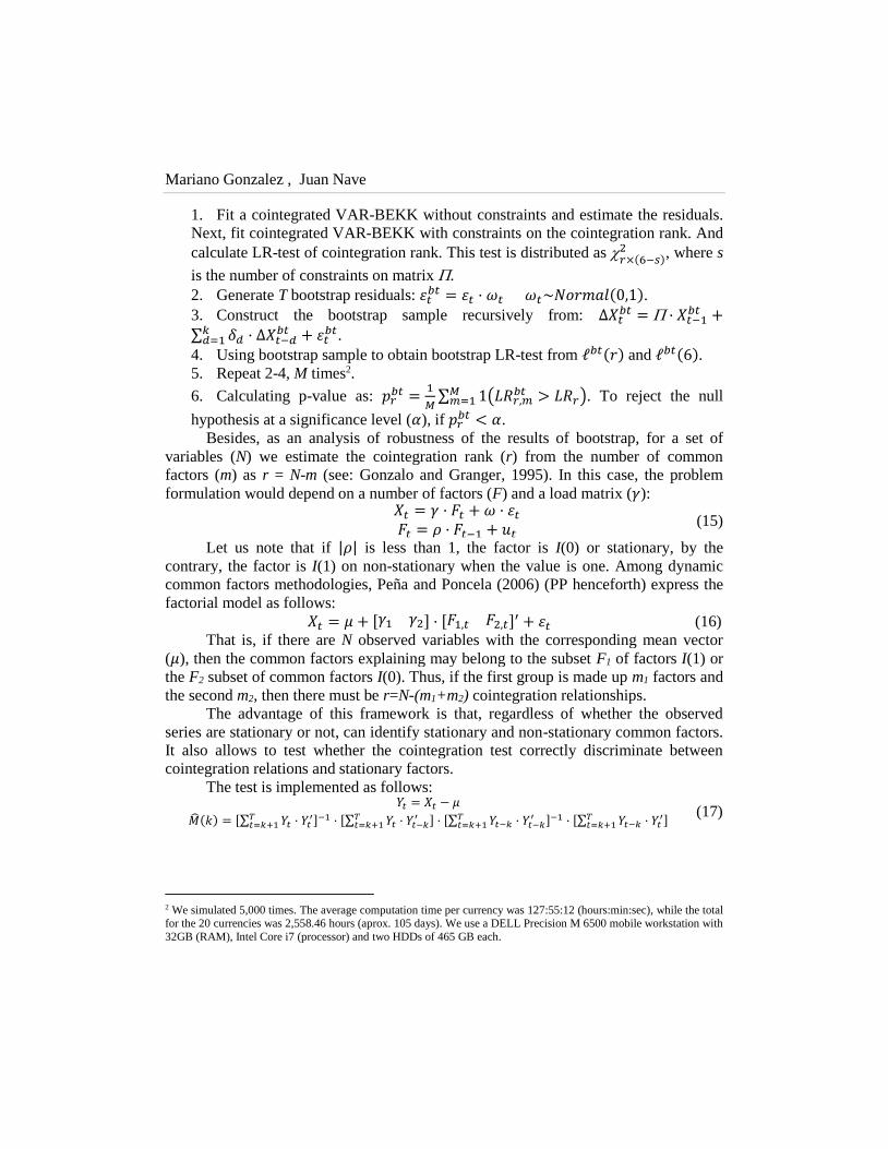
1. Fit a cointegrated VAR-BEKK without constraints and estimate the residuals.
Next, fit cointegrated VAR-BEKK with constraints on the cointegration rank. And
calculate LR-test of cointegration rank. This test is distributed as𝑟×(6−𝑠)2 , where s
is the number of constraints on matrix .
2. Generate T bootstrap residuals: 휀𝑡𝑏𝑡 = 휀𝑡 · 𝜔𝑡 𝜔𝑡~𝑁𝑜𝑟𝑚𝑎𝑙(0,1).
3. Construct the bootstrap sample recursively from: ∆𝑋𝑡𝑏𝑡 = · 𝑋𝑡−1
𝑏𝑡 +∑ 𝛿𝑑 · ∆𝑋𝑡−𝑑
𝑏𝑡𝑘𝑑=1 + 휀𝑡
𝑏𝑡.
4. Using bootstrap sample to obtain bootstrap LR-test from ℓ𝑏𝑡(𝑟) and ℓ𝑏𝑡(6).
5. Repeat 2-4, M times2.
6. Calculating p-value as: 𝑝𝑟𝑏𝑡 =
1
𝑀∑ 1(𝐿𝑅𝑟,𝑚
𝑏𝑡 > 𝐿𝑅𝑟)𝑀𝑚=1 . To reject the null
hypothesis at a significance level (𝛼), if 𝑝𝑟𝑏𝑡 < 𝛼.
Besides, as an analysis of robustness of the results of bootstrap, for a set of
variables (N) we estimate the cointegration rank (r) from the number of common
factors (m) as r = N-m (see: Gonzalo and Granger, 1995). In this case, the problem
formulation would depend on a number of factors (F) and a load matrix (𝛾):
𝑋𝑡 = 𝛾 · 𝐹𝑡 + 𝜔 · 휀𝑡
𝐹𝑡 = 𝜌 · 𝐹𝑡−1 + 𝑢𝑡 (15)
Let us note that if |𝜌| is less than 1, the factor is I(0) or stationary, by the
contrary, the factor is I(1) on non-stationary when the value is one. Among dynamic
common factors methodologies, Peña and Poncela (2006) (PP henceforth) express the
factorial model as follows:
𝑋𝑡 = 𝜇 + [𝛾1 𝛾2] · [𝐹1,𝑡 𝐹2,𝑡]′ + 휀𝑡 (16)
That is, if there are N observed variables with the corresponding mean vector
(𝜇), then the common factors explaining may belong to the subset F1 of factors I(1) or
the F2 subset of common factors I(0). Thus, if the first group is made up m1 factors and
the second m2, then there must be r=N-(m1+m2) cointegration relationships.
The advantage of this framework is that, regardless of whether the observed
series are stationary or not, can identify stationary and non-stationary common factors.
It also allows to test whether the cointegration test correctly discriminate between
cointegration relations and stationary factors.
The test is implemented as follows:
𝑌𝑡 = 𝑋𝑡 − 𝜇
(𝑘) = [∑ 𝑌𝑡 · 𝑌𝑡′𝑇
𝑡=𝑘+1 ]−1 · [∑ 𝑌𝑡 · 𝑌𝑡−𝑘′𝑇
𝑡=𝑘+1 ] · [∑ 𝑌𝑡−𝑘 · 𝑌𝑡−𝑘′𝑇
𝑡=𝑘+1 ]−1 · [∑ 𝑌𝑡−𝑘 · 𝑌𝑡′𝑇
𝑡=𝑘+1 ] (17)
2 We simulated 5,000 times. The average computation time per currency was 127:55:12 (hours:min:sec), while the total for the 20 currencies was 2,558.46 hours (aprox. 105 days). We use a DELL Precision M 6500 mobile workstation with
32GB (RAM), Intel Core i7 (processor) and two HDDs of 465 GB each.

Common Stochastic Trends and Efficiency in the Foreign Exchange Market
According to Peña and Poncela (2006) Theorem-3, the matrix (𝑘) has N-
(m1+m2) eigenvalue which converge in probability to zero as the sample size (T) tends
to infinity and the number of lags (k) increase such that k/T tends to zero.
In this way, the test is to sort the eigenvalue (𝜆) of the matrix (𝑘), and obtain
their sum as follows:
𝑆𝑚=𝑚1+𝑚2= (𝑇 − 𝑘) ∑ 𝑙𝑛(1 − 𝜆𝑗)𝑁−𝑚
𝑗=1 (18)
This sum behaves asymptotically as 𝑁−𝑚2 distribution, in our case N=6 and the
expected value of m is four.
4. Data
We use daily close Bid and Ask prices data on the exchange rate of the 20
currencies against USD and EUR (direct price3), from 1-july-2002 to 30-december-
2011 (2,478 observations per series from Reuters-3000 XTRA 4.5 platform of inter-
dealer market). As we consider Ask and Bid price, the number of series is 82. The Bid
price is the last reported offer price for a money instrument at 21:50 GMT, which is
part of bid/ask pair in a market maker driven market. While the Ask price is the last
(and best) reported buy price from a market maker at 21:50 GMT. The difference
between the Bid and Ask is known as the spread.
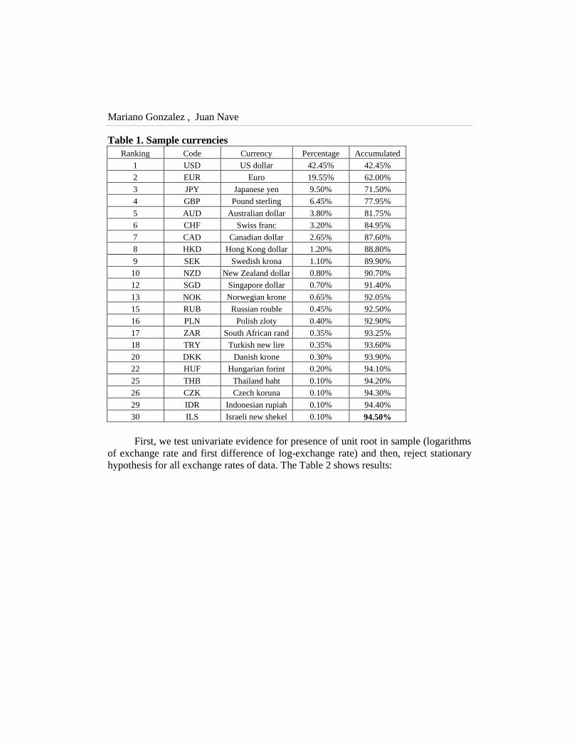
In Table-1 we show the sample currencies. It was selected of Triennial Central
Bank Survey, Foreign exchange and derivatives market activity in 2010 issued by
Bank for International Settlement (BIS, 2010, in Table 3, page 9]. We attempted at
percentage importance level, and the currencies are not traded directly against EUR are
excluded4:
3 We use those data to avoid the problems pointed out by Pasquariello (2001) when we work on indicative quotes. 4 In Reuters, some exchange rates against EUR are equals to triangular arbitrage prices and then, opportunities
arbitrages are not possible. These currencies are: Korean won, Taiwan dollar, Brazilian real, Chilean peso and Mexican
peso, because there is only a direct price of Mexican peso against EUR from 17-feb-2006.
Mariano Gonzalez , Juan Nave
Table 1. Sample currencies
Ranking Code Currency Percentage Accumulated
1 USD US dollar 42.45% 42.45%
2 EUR Euro 19.55% 62.00%
3 JPY Japanese yen 9.50% 71.50%
4 GBP Pound sterling 6.45% 77.95%
5 AUD Australian dollar 3.80% 81.75%
6 CHF Swiss franc 3.20% 84.95%
7 CAD Canadian dollar 2.65% 87.60%
8 HKD Hong Kong dollar 1.20% 88.80%
9 SEK Swedish krona 1.10% 89.90%
10 NZD New Zealand dollar 0.80% 90.70%
12 SGD Singapore dollar 0.70% 91.40%
13 NOK Norwegian krone 0.65% 92.05%
15 RUB Russian rouble 0.45% 92.50%
16 PLN Polish zloty 0.40% 92.90%
17 ZAR South African rand 0.35% 93.25%
18 TRY Turkish new lire 0.35% 93.60%
20 DKK Danish krone 0.30% 93.90%
22 HUF Hungarian forint 0.20% 94.10%
25 THB Thailand baht 0.10% 94.20%
26 CZK Czech koruna 0.10% 94.30%
29 IDR Indonesian rupiah 0.10% 94.40%
30 ILS Israeli new shekel 0.10% 94.50%
First, we test univariate evidence for presence of unit root in sample (logarithms
of exchange rate and first difference of log-exchange rate) and then, reject stationary
hypothesis for all exchange rates of data. The Table 2 shows results:

Common Stochastic Trends and Efficiency in the Foreign Exchange Market
Table 2. Stationarity Tests
Currencies
ADF test of LN(exchange rate) ADF test First difference of LN(exchange rate)
Ask_USD Bid_USD Ask_EUR Bid_EUR Ask_USD Bid_USD Ask_EUR Bid_EUR
EUR -2.563 [0] -2.56 [0] -- -- -50.09 [0] -50.14 [0] -- --
JPY -0.11 [16] -0.11 [16] -0.68 [30] -0.68 [30] -13.07 [15] -13.07 [15] -9.45 [29] -9.44 [29]
GBP -1.67 [1] -1.67 [1] -1.27 [4] -1.26 [4] -47.72 [0] -47.75 [0] -25.18 [3] -25.19 [3]
AUD -1.80 [13] -1.80 [13] -0.23 [22] -0.23 [22] -13.34 [12] -13.35 [12] -12.69 [21] -12.68 [21]
CHF -1.43 [24] -1.42 [24] 0.77 [35] 0.77 [35] -10.51 [23] -10.52 [23] -10.89 [34] -10.89 [34]
CAD -2.11 [34] -2.11 [34] -1.97 [0] -1.96 [0] -8.28 [33] -8.27 [33] -49.11 [0] -48.88 [0]
HKD -2.57 [19] -2.73 [18] -2.56 [0] -2.57 [0] -11.01 [18] -10.95 [18] -50.23 [0] -50.27 [0]
SEK -2.64 [9] -2.71 [8] -1.66 [49] -1.64 [49] -16.48 [8] -16.95 [7] -6.89 [48] -6.99 [48]
NZD -2.40 [4] -2.41 [4] -1.87 [3] -1.87 [3] -24.81 [3] -24.78 [3] -29.81[2] -29.84 [2]
SGD -0.59 [21] -0.59 [21] -1.31 [3] -1.31 [3] -12.08 [20] -12.15 [20] -31.07 [2] -31.09 [2]
NOK -2.42 [0] -2.42 [0] -2.55 [18] -2.55 [18] -36.68 [1] -36.75 [1] -12.08 [17] -12.09 [17]
RUB -2.05 [19] -2.05 [19] -1.75 [0] -1.74 [1] -9.06 [18] -9.06 [18] -51.46 [0] -51.54 [0]
PLN -2.13 [26] -2.04 [15] -1.45 [6] -1.45 [6] -9.61 [25] -9.69 [25] -23.89 [5] -23.90 [5]
ZAR -2.53 [15] -2.63 [11] -1.66 [0] -1.64 [0] -13.47 [14] -15.26 [10] -50.54 [0] -30.04 [2]
TRY -1.71 [4] -1.68 [4] -1.38 [1] -1.32 [3] -24.68 [3] -24.61 [3] -53.36 [0] -30.29 [2]
DKK -2.58 [0] -2.58 [0] -2.81 [5] -2.80 [5] -50.34 [0] -50.39 [0] -20.46 [5] -21.68 [4]
HUF -2.54 [0] -2.51 [0] -1.20 [6] -1.23 [6] -49.95 [0] -49.69 [0] -23.28 [5] -23.17 [5]
THB -1.12 [49] -1.16 [49] -2.26 [17] -2.08 [0] -7.40 [48] -7.16 [48] -10.63 [16] -51.18 [0]
CZK -1.72 [9] -1.70 [0] -1.15 [33] -1.13 [33] -16.35 [8] -11.17 [15] -8.82 [32] -8.78 [32]
IDR -2.26 [31] -2.24 [31] -2.37 [1] -2.39 [1] -9.57 [30] -9.59 [30] -57.97 [0] -59.43 [0]
ILS -1.61 [1] -1.49 [7] -2.72 [3] -2.72 [3] -47.01 [0] -19.78 [6] -31.58 [2] -31.67 [2]
Note: ADF tests are estimated with constant and a [number of lags] by information criteria AIC. Critical
values of rejection non-stationary are -2.86 and -3.44, at confidence levels of 5% and 1%, respectively.
We observe that the logarithm of exchange rates are non-stationary, while the
first difference of log (returns) is stationary, therefore, all data series in logarithms
have a unit root. Besides, it should be noted that the currencies of the Euro-zone have
higher lags against the euro to the dollar, while for the rest happens on the contrary,
except for NZD. In addition, except for the exchanges rates THB/EUR and ZAR/USD,
the bid prices showed more lags than ask. The exchange rates showing highest
difference in the number of lags between the bid and ask prices are: IDR/USD and
RUB/EUR.
In short, data show heteroskedasticity and autocorrelation, which fully justifies
the analysis of cointegration relations not only to lags that indicate the information test
(AIC), but also from significant lags (F-test), incorporating multivariate
heteroskedasticity (bootstrap BEKK) and by a supplementary dynamic factorial
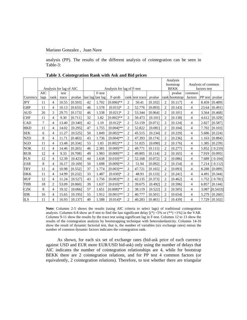
Mariano Gonzalez , Juan Nave
analysis (PP). The results of the different analysis of cointegration can be seen in
Table-3:
Table 3. Cointegration Rank with Ask and Bid prices
Currency
Analysis for lag of AIC Analysis for lag of F-test
Analysis
bootstrap
BEKK
Analysis of common
factors test
AIC
lags rank
test
trace pvalue last lag
F-test
last lag F-prob rank test trace pvalue rank
pvalue
bootstrap
common
factors PP test pvalue
JPY 11 4 10.55 [0.593] 42 1.702 [0.006]** 2 50.41 [0.102] 2 [0.117] 4 8.459 [0.489]
GBP 11 4 10.13 [0.633] 46 1.578 [0.015]* 2 52.776 [0.093] 2 [0.143] 4 23.64 [0.491]
AUD 26 3 29.75 [0.173] 46 1.538 [0.021]* 2 53.344 [0.064] 2 [0.101] 4 3.564 [0.468]
CHF 11 4 9.30 [0.711] 32 1.82 [0.002]** 2 50.473 [0.101] 2 [0.138] 4 4.612 [0.329]
CAD 7 4 13.40 [0.340] 42 1.19 [0.012]* 2 53.159 [0.071] 2 [0.124] 4 2.827 [0.587]
HKD 11 4 14.02 [0.295] 47 1.755 [0.004]** 2 52.822 [0.081] 2 [0.104] 4 7.702 [0.103]
SEK 6 4 11.27 [0.525] 50 1.849 [0.002]** 2 45.515 [0.234] 2 [0.229] 4 5.686 [0.224]
NZD 8 4 11.71 [0.483] 43 1.736 [0.004]** 2 47.393 [0.174] 2 [0.236] 4 1.163 [0.884]
SGD 11 4 13.48 [0.334] 53 1.83 [0.002]** 2 51.025 [0.090] 2 [0.176] 4 1.385 [0.239]
NOK 11 4 14.46 [0.265] 46 2.381 [0.000]** 2 49.771 [0.115] 2 [0.277] 4 5.852 [ 0.210]
RUB 12 4 9.33 [0.708] 49 1.983 [0.000]** 2 49.805 [0.114] 2 [0.165] 4 7.919 [0.095]
PLN 12 4 12.39 [0.423] 44 1.638 [0.010]** 2 52.168 [0.072] 2 [0.086] 4 7.689 [ 0.104]
ZAR 8 4 16.17 [0.169] 50 1.698 [0.009]** 2 51.94 [0.092] 2 [0.154] 4 7.214 [ 0.112]
TRY 11 4 10.98 [0.552] 37 1.774 [0.003]** 2 47.721 [0.165] 2 [0.093] 4 8.288 [0.089]
DKK 11 4 14.99 [0.232] 33 1.487 [0.030]* 2 48.93 [0.133] 2 [0.241] 4 4.491 [0.344]
HUF 12 4 11.24 [0.527] 43 1.756 [0.003]** 2 42.135 [0.373] 2 [0.462] 4 1.752 [ 0.781]
THB 18 2 53.09 [0.060] 39 1.637 [0.010]** 2 39.675 [0.492] 2 [0.596] 4 6.857 [0.144]
CZK 8 4 19.32 [0.066] 57 1.651 [0.008]** 2 38.119 [0.522] 2 [0.505] 4 3.087 [0.5433]
IDR 16 4 15.65 [0.195] 55 1.912 [0.001]** 2 40.777 [0.501] 2 [0.654] 4 5.279 [0.260]
ILS 11 4 16.93 [0.137] 40 1.588 [0.014]* 2 40.283 [0.461] 2 [0.439] 4 7.729 [0.102]
Note: Columns 2-5 shows the results (using AIC criteria to select lags) of traditional cointegration
analysis. Columns 6-8 show an F-test to find the last significant delay [(*) <5% or (**) <1%] in the VAR.
Columns 9-11 show the results by the trace test using significant lag in F-test. Columns 12 to 13 show the
results of the cointegration analysis by bootstrapping technique with heteroskedasticity. Columns 14-16
show the result of dynamic factorial test, that is, the number of variables (six exchange rates) minus the
number of common dynamic factors indicates the cointegration rank.
As shown, for each six set of exchange rates (bid-ask price of each currency
against USD and EUR more EUR/USD bid-ask) only using the number of delays that
AIC indicates the number of cointegration relationships are 4, while for bootstrap
BEKK there are 2 cointegration relations, and for PP test 4 common factors (or
equivalently, 2 cointegration relations). Therefore, to test whether there are triangular

Common Stochastic Trends and Efficiency in the Foreign Exchange Market
arbitrage opportunities, we consider that there are two cointegration relations, one for
the bid price and the other to ask.
5. Results
The null hypothesis of the lack of arbitrage opportunities is: (𝛽0,1 − 𝛽0,2) = 0.
In Table-4, we show LR-test on this hypothesis:
Table 4. LR test on constraints of arbitrage opportunities
Currency Beta constraint Chi^2(8) Beta+cost constraint Chi^2(9) Beta vs. Beta+cost Chi^2(1)
JPY 3.28 [0.916] 6.1 [0.73] 2.82 [0.093]
GBP 5.76 [0.674] 9.2 [0.419] 3.43 [0.064]
AUD 6.66 [0.574] 8.6 [0.475] 1.94 [0.164]
CHF 4.47 [0.812] 6.86 [0.651] 2.39 [0.122]
CAD 10.94 [0.205] 13.21 [0.153] 2.27 [0.132]
HKD 1.26 [0.996] 4.32 [0.889] 3.06 [0.081]
SEK 8.83 [0.357] 11.93 [0.218] 3.1 [0.078]
NZD 10.46 [0.234] 11.51 [0.242] 1.05 [0.306]
SGD 9.17 [0.328] 11.42 [0.248] 2.24 [0.134]
NOK 9.91 [0.272] 12.07 [0.21] 2.16 [0.142]
RUB 11.04 [0.199] 13.73 [0.132] 2.69 [0.101]
PLN 7.97 [0.437] 10.81 [0.289] 2.85 [0.092]
ZAR 4.04 [0.853] 5.6 [0.78] 1.55 [0.213]
TRY 12.85 [0.117] 15.89 [0.069] 3.04 [0.081]
DKK 8.24 [0.41] 11.5 [0.243] 3.26 [0.071]
HUF 7.57 [0.477] 11.27 [0.258] 3.7 [0.059]
THB 11.73 [0.164] 14.97 [0.092] 3.24 [0.072]
CZK 11.05 [0.199] 13.96 [0.124] 2.91 [0.088]
IDR 11.82 [0.16] 15.4 [0.081] 3.58 [0.058]
ILS 8.51 [0.385] 11.76 [0.227] 3.25 [0.072]
Note: This test is defined as: 𝐿𝑅 = −2 · [𝑙𝑜𝑔𝑙𝑖𝑘𝑟 − 𝑙𝑜𝑔𝑙𝑖𝑘𝑁]~𝑑𝑓2 , where loglik is log-likelihood for
general model (N) and model with r constraints; df is degree freedom. First column shows LR-test
between expression (9) and this general expression modified with beta constraint (10). Second column is
LR-test between expression (9) and modified model with beta and constant (cost) constraints. Third
column shows LR-test between modified expression with beta constraint, but with different and equal
constants (cost). The hypothesis null is rejected at 5% (*) or at 1% (**).
The results show that both price cointegration relationships (ask-bid) are defined
and that the assumption of arbitrage opportunities is rejected for all currencies.
Table-5 shows the daily rate of transaction costs estimated for each case:

Mariano Gonzalez , Juan Nave
Table 5. Daily rate of transaction cost
Currency
without restrictions beta restrictions cost equal
BID t-value ASK t-value BID tvalue ASK t-value CONSTANT t-value
JPY 0.02% 0.87 0.02% 0.92 0.02% 10.43** 0.02% 10.46** 0.02% 9.53**
GBP 0.02% 0.53 0.02% 0.26 0.02% 23.52** 0.02% 36.43** 0.02% 4.68**
AUD 0.04% 1.52 0.04% 2.57** 0.04% 28.94** 0.04% 41.34** 0.04% 9.28**
CHF 0.03% 6.15** 0.03% 6.16** 0.03% 2.37* 0.03% 2.38* 0.03% 2.82**
CAD 0.05% 13.84** 0.06% 13.76** 0.04% 0.03 0.04% 0.03 0.04% 5.40**
HKD 0.01% 11.43** 0.01% 11.49** 0.01% 11.07** 0.02% 11.07** 0.01% 9.58**
SEK 0.07% 16.40** 0.07% 16.22** 0.07% 5.52** 0.07% 5.55** 0.07% 5.57**
NZD 0.03% 3.92** 0.03% 4.13** 0.03% 41.01** 0.03% 38.02** 0.03% 6.31**
SGD 0.05% 17.13** 0.05% 17.14** 0.05% 11.84** 0.05% 11.86** 0.05% 5.16**
NOK 0.05% 2.67** 0.05% 2.67** 0.04% 3.12* 0.05% 3.14** 0.04% 3.08**
RUB 0.03% 4.30** 0.04% 4.24** 0.03% 15.45** 0.03% 15.42** 0.03% 14.02**
PLN 0.10% 0.17 0.10% 0.15 0.10% 7.04** 0.10% 11.92** 0.10% 10.97**
ZAR 0.16% 3.34** 0.16% 4.46** 0.17% 4.08** 0.17% 4.72** 0.17% 2.43*
TRY 0.16% 20.91** 0.16% 20.95** 0.15% 2.00* 0.15% 2.00* 0.15% 8.26**
DKK 0.02% 10.66** 0.02% 10.82** 0.02% 4.64** 0.02% 4.67** 0.02% 2.88**
HUF 0.11% 24.14** 0.11% 24.04** 0.12% 13.97** 0.12% 14.23** 0.12% 7.33**
THB 0.14% 0.93 0.14% 3.47** 0.13% 14.80** 0.13% 15.46** 0.13% 7.77**
CZK 0.10% 0.59 0.10% 0.6 0.10% 25.97** 0.01% 39.85** 0.11% 6.95**
IDR 0.14% 12.50** 0.14% 13.31** 0.13% 13.79** 0.14% 13.17** 0.13% 8.13**
ILS 0.14% 25.59** 0.14% 25.49** 0.14% 2.81** 0.14% 2.82** 0.14% 15.00**
Note: First column shows the rates of transaction cost to expression (9). The rate in second column are
estimated with expression (9) and the constraints of expression (10). Third column shows the estimated
rates under expression (9), (10) and an additional restriction on equality of transaction cost of ask and bid
prices, i.e. 𝛽0,1 = 𝛽0,2.The null hypothesis on transaction cost is rejected at 5% (*) or at 1% (**).
We observe that the model with a cost equal to the ask and bid ratio is
significant in all cases, and the cost is higher when the currency has less weight in the
global market.
6. Conclusions
This paper studies the foreign exchange market efficiency testing for the long-
run triangular arbitrage relationship among the spot exchange rate. The results show
evidence of no arbitrage opportunities. For doing this test, in opposite of others
authors, on the one hand, we have considered the micro-structure of spot exchange
market (daily bid and ask prices), i.e. the implicit transaction costs; and on the other
hand, using a unique database that represents more at 94% of total currency market
(USD, EUR and others 20 currencies).
Common Stochastic Trends and Efficiency in the Foreign Exchange Market
To overcome the problems arising from the use of high frequency data in
traditional cointegration test, we have employed a cointegrated VAR with a covariance
matrix heteroskedastic (BEKK) and we test the hypothesis according to a bootstrap
methodology and validate the results by a test of dynamic factors.
Our results lend empirical support to authors with respect to cointegration
relationship among exchange rates. But, contrary of others, we conclude that the null
hypothesis of non-arbitrage opportunities cannot be rejected. In conclusion, the spot
currency markets are cointegrated and so long-run arbitrage free, and as consequence
that, efficient.
REFERENCES
[1] Akram, Q., Rime, D. and Sarno, L. (2008), Arbitrage in Foreign Exchange
Market: Turning on the Microscope. Journal of International Economics, 76,
237-253;
[2] Baillie, R. T. and Bollerslev, T. (1989), Common Stochastic Trends in a
System of Exchange Rates. Journal of Finance, 44(1), 167-181;
[3] Bank for International Settlement (2010), Triennial Central Bank Survey.
Foreign Exchange and Derivatives Market activity in 2010. Available at:
http://www. bis.org/publ/rpfx10.pdf.
[4] Bos, C., Mahieu, R. and Van Dijk, H. (2000), Daily Exchange Rate
Behavior and Hedging of Currency Risk. Journal of Applied Econometrics,
156, 671-696;
[5] Caporale, G. M., Kalyvitis, S. and Pittis, N. (2001), Testing for PPP and
UIP in an FIML Framework: Some Evidence for Germany and Japan.
Journal of Policy Modelling, 23, 637-650;
[6] Cavaliere, G., Rahbek, A. and Taylor, R. (2010), Co-integration Rank
Testing under Conditional Heteroskedasticity. Journal of Econometric, 1581,
7-24;
[7] Cheung, Y. W. and Lai, K. S. (1993), Finite-sample Sizes of Johansen´s
Likelihood Ratio Tests for Cointegration. Oxford Bulletin of Economics, 553,
313-328;
[8] Choi, M. (2011), Monetary Exchange Rate Locked in a Triangular
Mechanism of International Currency. Applied Economics, 43(16), 2079-
2087.
[9] Chung, D.Y. and Hrazdil, K. (2012), Speed of Convergence to Market
Efficiency: The Role of ECNs. Journal of Empirical Finance, 19, 702-720;
[10] Crowder, W. J. (1994), Foreign Exchange Market Efficiency and Common
Stochastic Trends. Journal of International Money and Finance, 135, 551-
564;
Mariano Gonzalez , Juan Nave
[11] Diebold, F. X., Gardeazabal, J. and Yilmaz, K. (1994), On Cointegration
and Exchange Rate Dynamics. Journal of Finance, 49(2), 727-735;
[12] Dutt, S. and Ghosh, D. (1999), A Note on the Foreign Exchange Market
Efficiency Hypothesis. Journal of Economics and Finance, 232, 157-161;
[13] Fenn, D., Howison, S., McDonald, M., Williams, S. and Johnson, N.
(2009), The Mirage of Triangular Arbitrage in the Spot Foreign Exchange
Market. International Journal of Theoretical and Applied Finance, 128,
1105-1123;
[14] Fong, W., Valente, G. and Fung J. (2008), FX Arbitrage and Market
Liquidity: Statistical Significance and Economic Value. Working paper
08/2008, Hong Kong Institute for Monetary Research;
[15] Gagnon, L. and Karolyi, G. (2010), Multi-market Trading and Arbitrage.
Journal of Financial Economics, 971, 53-80;
[16] Gonzalo, J. and Granger, C.W.J. (1995), Estimation of Common Long-
memory Components in Cointegrated Systems. Journal of Business and
Economic Statistics, 13, 27-35;
[17] Johansen, S. (1988), Statistical Analysis of Cointegration Vectors. Journal of
Economic Dynamics and Control, 12, 231-254;
[18] Kollias, C. and Metaxas, K. (2001), How Efficient are FX Markets?
Empirical Evidence of Arbitrage Opportunities Using High-frequency Data.
Applied Financial Economics, 11, 435-444;
[19] Kozhan, R. and Tham, W. (2012), Execution Risk in High Frequency
Arbitrage. Management Science, 58(11), 2131-2149.
[20] Marshall, B. and Treepongkaruna, S. (2008), Exploitable Arbitrage
Opportunities Exist in the Foreign Exchange Market; Annual Meeting of
American Financial Association, New Orleans, 4-January;
[21] Martens, M. and Kofman, P. (1998),The Inefficiency of Reuters Foreign
Exchange Quotes. Journal of Banking & Finance, 22, 347-366;
[22] Moore, M. and Payne, R. (2011), On the Sources of Private Information in
FX Markets. Journal of Banking & Finance, 35(5), 1250-1262;
[23] Pasquariello, P. (2001), The Microstructure of Currency Markets: An
Empirical Model of Intra-day Return and Bid-ask Spread Behaviour.
Working paper, Stern School of Business, New York University;
[24] Peña, D. and Poncela, P. (2006), Nonstationary Dynamic Factor Analysis.
Journal of Statistical Planning and Inference, 1364, 1237-1257.
[25] Swensen, A. R. (2006), Bootstrap algorithms for testing and determining
the cointegration rank in VAR models. Econometrica, 74, 1699-1714.