astron. astrophys. 334, 953–968 (1998) astronomy …aa.springer.de/papers/8334003/2300953.pdf3...

Astron. Astrophys. 334, 953–968 (1998) ASTRONOMYAND

ASTROPHYSICS

Full spectrum of turbulence convective mixing:I. theoretical main sequences and turn-off for 0.6÷ 15 M�

Paolo Ventura1, Anna Zeppieri2, Italo Mazzitelli 1 and Francesca D’Antona3

1 Istituto di Astrofisica Spaziale C.N.R., Via del Fosso del Cavaliere, I-00133 Roma, Italy2 Collegio Leoniano, Anagni, Italy3 Osservatorio Astronomico di Roma, I-00040 Monteporzio, Italy

Received 12 December 1997 / Accepted 6 March 1998

Abstract. We present the results of extensive evolutionarycomputations from the Zero Age Main Sequence to the RedGiants, for stars in the range0.6 ÷ 15M� and with chemistry(Y , Z) = (0.274, 0.017). The novelty of these computations isin the general treatment of convection, namely:

1. convection as a whole is addressed in the Full Spectrumof Turbulence model (billions of eddy scales are considered)with the appropriate convective fluxes distribution, as opposedto the one-eddy Mixing Length Theory;

2. local chemical evolution also in the presence of convec-tion is separately evaluated for each element, as a result of a pro-cess in which nuclear evolution and turbulent transport are fullycoupled by means of a diffusive scheme (coupled-diffusion);

3. convective overshooting (when considered) is also ad-dressed in the above coupled-diffusive scheme, assuming thatthe turbulent velocity exponentially vanishes outside the for-mally convective region according to an e-folding free parame-ter ζ, tuned to fit observations.

After some tests on the small solar convective core in earlymain sequence, we discuss the effects of coupled-diffusion inthe cores of larger mass stars, where the nuclear lifetimes ofsome (p–p and) CNO elements can be comparable to the mix-ing times. We also compute a full grid of tracks with a smallamount of overshooting, finding thata unique free parametercan be suitable for the whole range of mass considered (solarand below solar included). Theoretical tracks are discussed, andisochrones are compared to the observational HR diagram forthe Pleiades, finding an age>∼ 120 Myr, consistent with thatobtained from the candidate brown dwarf PPL 15. An age isalso derived for the young clusterα Persei, for which a datationfrom the detection of lithium in brown dwarf candidates shouldbe soon available. For completeness, and to facilitate compar-isons with results by other authors, we also describe in detailstheATON 2.0 code used for the present computations.

Key words: stars: evolution of – convection – numerical meth-ods

Send offprint requests to: I. Mazzitelli

1. Introduction

In the vast majority of the stellar evolutionary computations uptoday, turbulent convection has been described as alocal mech-anism (in spite of its intrinsicnon-local character) accordingto the Mixing Length Theory (MLT). In the local approxima-tion, at the Schwarzschild boundary both velocity and acceler-ation go to zero together with the buoyancy forces acting on theconvective elements, and nothing can be known about the tur-bulent velocity profiles outside formally convective regions. Inaddition, in convective and overshooting regions instantaneouschemical mixing decoupled from nuclear evolution is generallyassumed in stellar modeling, with the only noticeable exceptionof Sackmann et al. (1995) for the external layers of AsymptoticGiant Branch (AGB) stars, where coupling nuclear evolutionand mixing is the only correct way of describing the surfacelithium evolution.

And yet, both overshooting and chemical evolution in tur-bulent regions do affect the behavior of stars. Let us first con-sider overshooting alone. Some attempts have been made topredict – very often according tonon-localcorrections to theMLT – the amount of mixed matter (Shaviv & Salpeter 1973;Roxburgh 1978, Xiong 1985, Grossman 1996 etc.); many suchmodels have been reviewd and criticized on theoretical groundsby Canuto (1992, 1996). When constructing stellar models,all the above approaches predict large overshooting distances(∼ 1.4 ÷ 1.8Hp, beingHp the pressure scale heigth) whichshould lead to dramatic – and not observed – consequences atleast on the evolution of massive stars in young open clusters(Maeder 1990).

Computations with a bare parametric approach to the prob-lem have been then also tried, allowing instantaneous mixingbeyond the formal convective borders up to a fraction ofHp (e.g.Maeder & Meynet 1987; Stothers & Chin 1992). According toMaeder & Meynet (1991), the main sequences of young clus-ters are reasonably fit with an instantaneous overshooting fromthe convective corelov ∼ 0.25Hp; for older clusters (Turn Off(TO) masses< 1.6M�) the temporal evolution of the convec-tive cores is more tricky, depending on details of the chemicaland physical inputs (Maeder & Meynet 1987). An analogous

954 P. Ventura et al.: Full spectrum of turbulence convective mixing: I.

upper value to overshooting (lov ∼ 0.20Hp) has been also sug-gested by Stothers & Chin (1992).

As for non-instantaneousmixing (and overshooting), Denget al. (1996a,b, always in an MLT framework) suggested that itis more physically realistic to expect smooth chemical profilesoutside the convective boundaries, consistent with a diffusivedescription of the process. In the present paper we adopt a dif-fusive approach too, with considerable conceptual differenceswith respect to all the previous studies to be discussed in detailsin the following.

As for the effects of coupling nuclear evolution to non-instantaneous mixing, we only found sparse references in theliterature to the problem as a whole, and to possible rough so-lutions with complete mixing if nuclear lifetimes are longerthan mixing times, locally frozen compositions in the oppositecase. In the best of our knowledge, the present computationsare the first ones in which the problem has been consistentlyand extensively addressed, apart from the already quoted caseby Sackmann et al. (1995) in AGB. Full Spectrum of Turbu-lence (FST) convection model, and coupling between nuclearevolution and diffusive mixing, are then the main differencesbetween the present paper and all the preceding literature.

2. The convective model

2.1. Convection as a whole

A short discussion on the convective model adopted in thepresent computations is unavoidable, since the results obtainedwith diffusive mixing depend on the convective velocities andscale lengths.

Convection in stars is by far turbulent, the largest eddieshaving a size comparable to that of the entire convective region(∼ 109 ÷ 1012 cm). They break down pumping (downscat-ter) and getting back (backscatter) kinetic energy into smallereddies, until molecular viscosity takes over, and the kinetic en-ergy stored in the whirlpools is thermally dissipated; billions ofeddy scales are then present in stars. Navier–Stokes equationsdescribing this process from first principles are both non-linearand non-local (Xiong 1985, Canuto 1992, Grossman 1996), andtheir analytical or numerical solution for a general stellar case isnot yet available. In stellar modeling, we then still stick tolocalmodels to compute both the energy fluxes and the convectivescale lengths.

As for the fluxes, MLT (Prandtl 1925) – originally devel-opped for very viscous fluids – was first applied by Vitense(1953) to stellar modeling. In the MLT, the spectral distributionof eddies is mimicked by one “average” eddy only. More up-dated models provide now fluxes also for low-viscosity flows,in which the whole eddy spectrum is accounted for (Canuto &Mazzitelli 1991 and 1992, Canuto et al. 1996–CGM). Stothers& Chin (1995) defined Full Spectrum of Turbulence (FST) theselatter models, as opposed to the one-eddy spectrum MLT. In thepresent work we adopt the FST scheme with the CGM fluxes.

The scale lengthΛ was originally chosen, in the MLT, coin-cident with the distancez from the convective boundary, consis-tently with Von Karman law for incompressible fluids (Prandtl

1925). Since however the one-eddy flux distribution is verycrude, no realistic fit of the Sun could be obtained. It is thennow customary to apply the MLT withΛ = αHp, whereα isa free parameter tuned on the solar model; depending on themicro-physical inputs,1.5 ≤ α ≤ 2.2.

The more physically correct choiceΛ = z close to the con-vective boundaries is instead allowed in an FST framework.However, far from the boundaries, alsoΛ must, in a star, ap-proach the hydrostatic scale lengthHp. To match these require-ments, we consider both the upper and the lower convectiveboundary; we compute for each convective grid pointzup andzlow and assumez as their harmonic average. Close to theboundariesz ' zup or ' zlow, which is the required result.For deeper layers, let us recall that, in a polytropic structure ofindexn, z ≈ (1 + n)Hp (Lamb 1932). In convective regionsn ∼ 1.5, that is:z ∼ 2.5 · Hp. The harmonic average givesz ≡ zup/2 ≡ zlow/2 ∼ 1.25 · Hp, again close to the requiredvalue.

No perfecttheory of convection, however, still exists, andthe same is true for all other micro/macro-physical inputs. If wethen ask for anexactfit of the Sun, some tuning of the modelsis required. With the MLT,all the physical uncertainties areusually reset by means of thecompletelyfree parameterα. Atvariance, in an FST environment we recall thatΛ should alsoallow for overshooting (Λ = z + OV ), which is not yet knownfrom first principles. We can then parametrizeOV = βHtop

p

(or OV = βHbotp ), such thatβ can be seen as afine tuning

parameter, constrained by0 ≤ β ≤ 0.25 (Maeder & Meynet1991, Stothers & Chin 1992). Note that FST tuning affects onlylayers close to the boundaries since, for inner layers,z fastlygrows� OV . With CGM fluxes (Kolmogorov constant updatedto Ko = 1.7) the solar fit requiresβ ∼ 0.1, the value slightlydepending on the chemical abundance chosen. WithOV = 0one would get an underestimate of the solarTeff around 1.5%;too much for helioseismological purposes, but almost negligiblein the more general framework of stellar evolution. In the presentpaper we will always adopt

Λ = zup · zlow/(zup + zlow)

unless differently specified, wherezup is the distance from thetop of convection increased byβHtop

p , and analogously forzlow.

2.2. Diffusive mixing and overshooting

According to first principles, in the presence of both nuclearreactions and turbulent mixing, the local temporal variation oftheith element follows the diffusion equation (Cloutman & Eoll1976):(

dXi

dt

)=

(∂Xi

∂t

)nucl

+∂

∂mr

[(4πr2ρ)2D

∂Xi

∂mr

]. (1)

stating mass conservation of elementi if molecular diffusionbe negligible with respect to turbulent diffusion (almost alwaystrue). The diffusion coefficient D is:

D = 16π2r4ρ2τ−1 (2)

P. Ventura et al.: Full spectrum of turbulence convective mixing: I. 955

whereτ , the turbulent diffusion timescale, is related to the one-point density-radial velocity correlation

< ρ′iu

′ >= −τ∂ρi/∂r (3)

Unfortunately, knowledge of the second order momentum inEq. (3) requires previous solution of the Navier-Stokes Eqs. fora compressible stellar fluid, not yet available in the huge varietyof cases of astrophysical interest. Also forD a local approxi-mation is then customarily used, that is:D = uld/3, whereuis the average turbulent velocity andld (= Λ in the formallyconvective region) is the convective scale length.

In an MLT framework, the above approximation is highlydisputable since experiments show that turbulent chemical mix-ing is more efficient at thesmallestscales, at variance with theunique (largest) MLT scale. More physically sound is the FSTdescription: the average velocity accounts also for the smallesteddies, and the scale length is always the more correct one. Inour case we then expect to get a better approximation to the“true” diffusion coefficient.

Turbulent velocityu is computed according to Eqs. (88),(89) and (90) by CGM. One problem arises because of the “lo-cality” of the FST model (u at the convective boundaries van-ishes). However,u sharply goes to zero only very close to theboundaries; a little deeper in the convective region, the velocityprofile approaches to a plateau. It is then possible to extrapolatea “reasonable” non-vanishing velocity at the formal boundary,and test computations starting from a pressure either 2%, 5%or 10% inside the boundary gave almost identical results. Wethen extrapolatelog u vs. log P to get the turbulent velocity atthe formal boundary starting from a pressure 5% inside.

As for diffusive overshooting (if any) we recall that, accord-ing to Xiong (1985), turbulent velocity exponentially vanishesoutside formally convective regions. We then write, in over-shooting regions:

u = ub exp±(

1ζfthick

lnP

Pb

)(4)

whereub andPb are respectively turbulent velocity and pressureat the convective boundary,P is the local pressure,ζ is a freeparameter to be tuned as discussed in the following, andfthick isthe thickness of the convective region in fractions ofHp (max-imum value offthick = 1), to maintain a non-locality flavor,sincefthick scales overshooting according to the thickness of theconvective region. While the diffusive scale length in formallyconvective regions is obviouslyld = Λ as in Sect. 2.1, in theovershooting regions we useld = βHp to maintain continuityof the diffusive coefficient D at the boundaries.

In a first approximation, then, our framework for diffusivemixing and overshooting shows similarities to the one by Denget al. (1996a,b). However:

a) use of FST instead of MLT, with different diffusive ve-locities and scale lengths, leads to different results, and:

b) the chemical evolutionary scheme is far different in ourcase, since we fully couple nuclear evolution and diffusive mix-ing (hereafter to: “coupled-diffusion”).

Of course,ATON 2.0 code also allows computations withinstantaneous mixing and overshooting (in this latter case, theovershooting distance is simplyνHp as usual). In the follow-ing, comparisons between results obtained with instantaneousmixing and coupled-diffusion will be presented.

2.3. Coupled mixing and nuclear evolution

When using Eq. (1) two alternatives choices could be made:a) numerically evaluate(∂Xi/∂t)nucl as a function of local

abundances and cross sections, substitute in Eq. (1) and onlythen apply the diffusive algorithm. The bonus of this choiceis that the problem is reduced to a “semi-local” one: no largematrices must be stored and computations are relatively fast.The drawback is that nuclear evolution is completely decoupledfrom mixing, and some mechanisms –like hot bottom burninglithium production in the envelopes of AGB stars (Sackmann etal. 1995), or effect of mixing on the CNO equilibria – cannoteven be addressed;

b) analytically expand(∂Xi/∂t)nucl as a function of lo-cal abundances and cross sections, and solve it together withthe diffusion matrix for the whole stellar structure. Ifchem isthe number of chemical species andgrid is the number of gridpoints, a matrix of rank(chem · grid) × (chem · grid) – typ-ically 100 ÷ 500 MB – must be stored and inverted. Methodb) severely threatens any workstation, but correctly couples nu-clear evolution to the contemporary change of composition dueto turbulent transport of matter (coupled-diffusion).

We then made choice b) which, after some algebraic manip-ulations fully described in Sect 9.4, can be reduced to the storageand inversion of a matrix of rank(3 · chem) × (chem · grid) –typically ∼ 1 ÷ 3 MB – well affordable according to safe andfast algorithms. For more details on the nuclear evolutionaryscheme as a whole, see Sect. 9.3.

3. Micro-physical inputs

Since comparisons with former results by different authors willturn out somehow elusive due to our previously untested evolu-tion/convection/mixing combination, we felt obliged to at leastsummarize and shortly describe the micro-physical inputs inATON 2.0. In the Appendix, also the main numerical featuresof the code will be addressed.

3.1. Thermodynamics

Thermodynamics tables are given as a function of temperatureand pressure. InATON 2.0 they are built, for any given metalabundanceZ, in three steps.

First, the tables by Magni & Mazzitelli (MM 1979, recentlyupdated in full ionization regime) are stored for the fiveH–abundances:X = 1.0 − Z; X = .8 − Z; X = .5 − Z; X =.2 − Z; X = 0.0. Since MM tables were computed forZ = 0,an “average” metal is interpolated from the pure-carbon tableby Graboske et al. (1973). This latter procedure satisfactorilymimicks an EOS with metals at least as long asZ ≤ Z�. A


former release of MM EOS has been however shown by Saumon(1994) somewhat biased in high-T, low–ρ regions, while theP = P (ρ, T ) relation performs fairly well in the low-T, high–ρnon-ideal gas regime.

A severe warning is here necessary: contrarily to some morerecent EOS’ for non-ideal gas (e.g. Saumon et al. 1995), MMthermodynamics has been computed not only forpureH or Hechemical compositions, but also forH/He mixtures. In spite ofits age, it is then still more physically updated than other EOS’in pressure dissociation and ionization domain, where interpo-lation (with the additive volumes law or any other such scheme)betweenpureelements is bound to give unreliable results, dueto thephysicalinfluence ofH-ions on theHe-bound states.

As a second step, the tables (covering theρ-T plane up todensities where the lattice ion quantum effects begin to showup) are partially overwritten by the Mihalas et al. (MHD, 1988)equation of state, for the chosen Z and in the range LogT ≤ 5;Log ρ ≤ −2. MHD EOS is in fact biased (Saumon 1994) atlarger densities, where the MM EOS is instead still quite good.With this second step, correct allowance forZ is obtained in thelow-T, nearly ideal gas region, but for the uniqueH/He ratiofor which the MHD EOS are provided.

Third and final step: the above tables are partially overwrit-ten by the OPAL EOS tables (Rogers et al. 1996) where available(3.7 ≤ LogT ≤ 8.7), for the same fiveH/He ratios as in MM.In this way, residual anomalies (if any) at high-T in the MMEOS are forgotten, and variableH/He ratios are restored in allthe cases of interest.

Lastly, one pure-carbon and one pure-oxygen table, com-puted in full ionization regime with an improved MM-likescheme, are addedd. Bicubic logaritmic interpolation on bothP and T are performed on the tables at fixed H-abundances,and linear interpolation on the chemical composition follows,to evaluate the various thermodynamical quantities.

3.2. Opacity

A procedure similar to the above one is performed also for theopacities. For each givenZ, OPAL opacities (Rogers & Igle-sias 1993), linearly extrapolated (log κ vs. log ρ) in the high–ρregion, and harmonically added to conductive opacities (Itoh &Kohyama, 1993), form the ground level.

At lower temperatures (T < 6000K), Alexander & Fer-guson’s (1994) molecular opacities (plus electron conductionwhen in full ionization) complete the tables, for the same 10H/He ratios as in OPAL’s case. At variance, Kurucz (1993)low temperatures (T < 6000K) opacities can be used, but foroneH/He ratio only.

For He/C/O mixtures, interpolation on fifteen out of the60 OPAL tables (plus conductive opacities) is performed. Com-parisons with the full set of 60 tables show that, with the presentreduced set, interpolation on the chemical composition alwaysgives agreement better than2% and, in the vast majority ofcases, better than1%. Bicubic logaritmic interpolation on bothρ andT are performed on the tables at a fixedH/He ratio, and

quadratic interpolation onH follows to get the final opacityvalue.

3.3. Nuclear network

It includes the 14 elements:1H, 2H, 3He, 4He, 7Li, 7Be, 12C,13C, 14N , 15N , 16O, 17O, 18O, 22Ne. We explicitly considerthe following 22 reactions:

p + p −→2 H + e+ + νp + p + e− −→2 H + ν2H + p −→3 He + γ3He +4 He −→ α + 2p3He +4 He −→7 Be + γ7Li + p −→ 2α7Be + p (−→8 B + γ −→8 Be) −→ 2α7Be + e− −→7 Li + γ12C + p (−→13 N + γ) −→13 C + e+ + ν13C + p −→14 N + γ14N + p (−→15 O + γ) −→15 N + e+ + ν15N + p −→ α +12 C15N + p −→16 O + γ16O + p (−→17 F + γ) −→17 O + e+ + ν17O + p −→ α +14 N17O + p (−→18 F + γ) −→18 O + e+ + ν18O + p −→15 N + α3α →12 C + γ12C + α →16 O + γ14N + α(→18 F + γ) −→18 O + e+ + ν12C +12 C → α/2 +22 Ne18O + α →22 Ne + γ

The reactions in parentheses are so fast that they are notexplicitated (in terms of mixing, the half-lifes of the elementsare so short that they are always inlocal equilibrium). The crosssections for the other reactions are from Caughlan & Fowler(1988); low, intermediate and strong screening coefficients arefrom Graboske et al. (1973). The12C +12 C reaction has beengiven a fictitious end inα/2 +22 Ne, sinceATON 2.0 codecan follow12C-ignition, but has not been set to deal with moreadvanced evolutionary phases.

Logaritmic nuclear cross sections are in tables with a verythin spacing in LogT , and are cubically interpolated.

3.4. Neutrinos

Pair, photo, bremsstrahlung and plasma neutrino have beentaken from Itoh et al. (1992). Recombination neutrinos havenot been included, since they are of interest only for more ad-vanced (pre-supernova) evolutionary phases, which presentlylie out of the domain ofATON 2.0.

Due to the computing time required to evaluate the variousneutrino fluxes with the fitting formulae in the literature, webuilt up logaritmic tables of neutrino rates for various elements.Bicubic logaritmic interpolation on bothρ andT are performedon the tables at a fixed chemistry, and linear interpolation on thechemistry follows to compute the neutrino emission.


3.5. 4He sedimentation

Also gravitational settling and chemical and thermal diffusionof 4He is optionally included inATON 2.0. To avoid confusionwith the termdiffusion, for which we prefer to maintain themeaning ofmixing due to turbulent convection, in the future,we will refer to all the processes leading to4He settling assedimentationtout court.

The following approximations are made, consistently withMuchmore (1984) and Paquette et al. (1986):

- radiative force can be neglected- all particles, including the electrons, have approximately

Maxwellian distribution- mean thermal velocities are much larger than the diffusion

velocities- magnetic fields are absent.

The sedimentation velocities then satisfy (Proffitt & Mi-chaud 1991; Paquette et al. 1986):

d pa

dt− ρa

ρ· d p

dr− naZaeE

=∑

j

Kaj(wa − wj) +nanj

na + njαT k

d T

dr(5)

wherepa, ρa, na, Za, wa are the partial pressure, mass density,number density, mean charge, and sedimentation velocity forspeciesa (in our case, respectively:1H, 4He and electrons),andE is the electric field induced by the gradients in ion densi-ties (Aller & Chapman 1960). The resistance coefficientsKaj

are taken from a fit (Iben & Mc Donald 1985) of the numeri-cal results by Fontaine & Michaud (1979), while for the totalthermal diffusion we adoptαT = 2.54Z2

2 − .804Z2 (Alcock &Illarianov 1980).

In terms of temperature gradient and number density, Eq. (5)may be rewritten as:

1na

∑j

Kaj(wa − wj) − ZaeE

= −AamHg − kTd lnT

dr+ αT

nj

na + njk

d T

dr− kT

d lnna

dr

whereAa is the molecular weight for theath species, whilemH

is the hydrogen mass.To complete the set of equations we apply the condition for

no net mass flow relative to the center of mass and no electricalcurrent. To proceed, we separate out the velocity thermwa as:

wa = wgta −

∑j

σajd lnnj

dr,

wherewgta is relative to the gravity components and temperature

gradient, while the summatory is relative to the components dueto gradients in number densities, that is:

wgt1 =

G + H

D; wgt

2 = −G + H

D· α1

α2

where all the symbols have the same meaning as in Iben & Mc-Donald (1985) but forH (due to thermal diffusion, not presentthere):

H = α2

[(n2β1 − n1β2) − αT · n1n2

n1 + n2(β1 − β2)

]k

dT

dr.

We then use these expressions in the continuity equation:

∂ na

∂t= − 1

r2

∂

∂r

r2

wgt

a −∑

j

σajd lnnj

dr

which can be solved by a conservative, semi-implicit finite dif-ference method of first-order in time and second-order in thespatial variabler, always following the procedure by Iben &Mc Donald (1985).

4. The solar model

4.1. The early convective core

We first computed a bunch solar evolutionary tracks with metalabundancesZ = 0.017 and Z = 0.020, bracketing the ac-tual value ofZ� (Grevesse 1984; Grevesse & Noels 1993). Westarted from homogeneous main sequence and followed evolu-tion up to an age of∼ 5 Gyr, slightly larger than the presentlyaccepted solar age of4.6 ± 0.1 Gyr. Pre-main sequence phaseswith deuterium burning were not accounted for; so we startedthe computations with no3He. The initial 4He abundanceY0was adjusted for each track to fit the observed solar luminosity,and the fit of the observed radius was achieved by fine tuningof the FST parameterβ.

In all, 20 tracks were computed as detailed in Table (1).In all theν > 0 cases, instantaneous mixing and overshooting(Λov = νHp) were present; whenζ > 0 coupled-diffusion plusovershooting (Eq. (4)) were adopted. Theν = ζ = 0 case canbe seen as representative of both instantaneous mixing and/orcoupled-diffusion, since for the small solar convective core inearly main sequence both treatments give almost exactly thesame results. For larger mass stars, when CNO burning in con-vective core dominates the structure, the case is different as wewill see later on.

Some of the main results are shown in Table (2), where alsothe thickness of the external convective envelope (in fractionsof the solar radius) and the present surface helium abundance(when sedimentation is active) are reported. Note en passantthat models with Z=0.020 and sedimentation seem to better fitthe helioseismologically “observed” thickness of the convectiveenvelopeRconv = .287 ± .003R� (Christensen–Dalsgaard etal. 1991). Conclusions about the solar metal abundance fromthese data would be however premature, since any further smallrevision of radiative opacities, or even an overshooting from thebottom of convection by a few thousand Km (smaller than theupper limit of ∼ 0.05Hp suggested by Basu & Antia, 1997)could still change the picture.

For completeness, we also show in Table 3 the neutrinofluxes in SNU predicted for all the solar models computed.


Fig. 1. Evolution of the initial solar convective core versus time, forvarious choiches of theζ (diffusive overshooting) orν (instantaneousovershooting) parameter. The larger is the extra-mixing, the longer theduration of the convective core

Table 1.Legend of the labels for the evolutionary sequences computed.For the ten choices of convection modeling and diffusion displayedwith the last digit, the two choices of metallicities are displayed by thepenultimate digit

Track νinst.ov. ζdiff.ov. sed.

SUNX0 0.0 0.000 NOSUNX1 0.05 0.000 NOSUNX2 0.1 0.000 NOSUNX3 0.2 0.000 NOSUNX4 0.0 0.010 NOSUNX5 0.0 0.020 NOSUNX6 0.0 0.040 NOSUNX7 0.0 0.010 YESSUNX8 0.0 0.020 YESSUNX9 0.0 0.040 YES

SUN0Y Z=0.017SUN1Y Z=0.020

Our results are largely consistent with those by Bahcall & Pin-sonneault (1992), both with and without helium sedimentation.Overshooting, even if slightly changing the central3He abun-dances as discussed in the following, does not substantially mod-ify the 7Be fluxes, also because the more than 80% of the solar3He is consumed via the3He +3 He channel.

Let us now discuss the behavior of the small, early solarconvective core, as depicted in Fig. 1 for the Z=0.017 case (theZ=0.020 case shows only small quantitative differences). Evenif the argument is not a strict novelty, it will help to elucidate

Table 2.Thickness of the convective envelope and4He abundance atthe surface of the models computed. The second and fifth columns givethe initial 4He abundance adopted to fit the present solar luminosity

Model Y0 Rc \ R� Ys Model Y0 Rc \ R� Ys

SUN00 0.269 0.273 SUN10 0.282 0.280SUN01 0.270 0.275 SUN11 0.282 0.285SUN02 0.270 0.278 SUN12 0.282 0.288SUN03 0.272 0.287 SUN13 0.284 0.296

SUN04 0.269 0.274 SUN14 0.282 0.280SUN05 0.269 0.274 SUN15 0.282 0.281SUN06 0.269 0.274 SUN16 0.282 0.280

SUN07 0.271 0.277 0.2602 SUN17 0.284 0.283 0.27313SUN08 0.271 0.276 0.2613 SUN18 0.284 0.283 0.27435SUN09 0.271 0.276 0.2629 SUN19 0.284 0.283 0.27595

the qualitative differences between instantaneous and diffusiveovershooting.

At the beginning of ZAMS, when LogTc ∼ 7.15, the ini-tial 12C abundance is quite large (12C/Z ∼ 0.18), and trans-formation of 12C into 14N is responsible for the generationof ∼ 10% of the total luminosity very close to the center(σ(12C + p) ∝ T 18, very stiff with T ). TheL/r2 ratio (andthe radiative gradient) is sufficiently large to keep alive a con-vective core.12C is then consumed and convection tends to diein ∼ 70 ÷ 80 Myr (test computations with initial12C = 0 donot show a very early convective core).

In the meantime,3He begins to be produced; its equilibriumconcentration reaches a maximum and, when12C is exhaustedandTc increases to allow thep − p chain to fully power thestar, also central3He decreases. Since(σ(3He+3 He) ∝ T 15,again quite stiff), a “large” abundance of3He could keep alive aconvective core too. Actually, central conditions in the Sun (andalso in stars of mass up to∼ 1.2M�) turn out such that, when thep − p chain takes over, the central equilibrium concentration of3He is just slightly smaller than that required to maintain centralconvection. At this very point the presence of overshooting canplay a role, as discussed in the next section.

4.2. Instantaneous vs. diffusive overshooting

In general solar conditions, the lower isT , the larger the equi-librium abundance of3He, which is then minimum at the centerof the star and increases outwards, reaching a peak abundancearound∼ 0.3 ÷ 0.4M�. Overshooting, then, mixes the corewith surrounding matter overabundant in3He with respect tothe central equilibrium concentration. This leads to overproduc-tion of luminosity, maintaining large the radiative gradient andconvection alive.12C is ineffective for this purpose since, onceburned, is not produced any more. Figure 2 shows the small dif-ference in3He abundance profiles with and without diffusiveovershooting, sufficient to make the difference between an earlydeath and a prolonged existence of a convective core.


Table 3. Computed neutrino fluxes. Results are expressed in SolarNeutrino Units (SNU)

Model φ(pp) φ(pep) φ(7Be)φ(8B) φ(13N) φ(15O) φ(17F )1010 108 109 106 108 108 106

SUN00 6.060 1.380 4.080 4.364 3.298 2.672 3.205SUN01 6.081 1.384 4.130 4.550 3.332 2.679 3.222SUN02 6.085 1.383 4.331 4.708 3.542 2.887 3.525SUN03 6.072 1.356 4.473 3.630 3.698 3.067 3.785SUN04 6.064 1.382 4.106 4.425 3.329 2.704 3.244SUN05 6.065 1.382 4.104 4.426 3.325 2.699 3.245SUN06 6.059 1.379 4.089 4.463 3.330 2.701 3.253SUN07 6.074 1.378 3.982 4.180 3.105 2.497 2.983SUN08 6.075 1.379 3.984 4.185 3.105 2.497 2.985SUN09 6.075 1.379 4.008 4.306 3.152 2.544 3.052SUN10 5.992 1.348 4.534 5.485 4.558 3.825 4.674SUN11 5.977 1.342 4.600 5.800 4.660 3.924 4.834SUN12 5.996 1.347 4.880 5.954 4.967 4.212 5.259SUN13 5.977 1.320 5.050 4.780 5.190 4.466 5.641SUN14 5.994 1.348 4.540 5.498 4.563 3.830 4.683SUN15 5.997 1.349 4.559 5.553 4.591 3.858 4.724SUN16 5.992 1.348 4.553 5.612 4.605 3.869 4.747SUN17 6.008 1.347 4.4314 5.252 4.268 3.560 4.333SUN18 6.007 1.347 4.447 5.270 4.264 3.555 4.330SUN19 6.007 1.347 4.449 5.366 4.311 3.604 4.401

Let us finally discuss the different behaviors of the con-vective core with either instantaneous or diffusive overshoot-ing. In the former case, the mixing boundary is plainly shiftedoutwards. According to the present results, instantaneous over-shooting of∼ 0.10Hp would suffice to give a steady convec-tive core for the Sun untilH-exhaustion and, in turn, to a de-tectable gap at the Turn-Off of old open clusters. Consistentlywith Maeder & Meynet (1987), we conclude that an overshoot-ing this large must be excluded for solar mass stars.

More tricky is the case of diffusive overshooting, where mix-ing is a somewhat slow process which is almost complete onlyclose to the Schwarzschild boundary, exponentially vanishing atlarge distances. For the Sun, diffusion withζ ∼ 0.02 is roughlysimilar to instantaneous mixing withν ∼ 0.05 (Fig. 1). And yet,no strictequivalencecan be established, since a detailed anal-ysis of the numerical results shows that, withζ ∼ 0.02, partialdiffusive mixing reaches farther than0.05Hp beyond the formalconvective boundary.

This test gives an hint about the profound differences be-tween the two parametersν and ζ: to get almost the sameamount of mixed matter, the numerical value of the latter mustbe lower than that of the former. Moreover, in the solar casefthick ≤ 0.25. According to Eq. (4) it is then likely that, formore massive stars with large convective cores (fthick = 1), in-stantaneous overshooting withν ∼ 0.2 should bealmost equiv-alent to diffusive overshooting withζ ∼ 0.02 as long as theamount of mixed matter is concerned. We then conclude that:

a) with diffusive overshooting,ζ ∼ 0.02 is a conservativeestimate which does not modify the overall framework of solar

Fig. 2.The3He abundance profile (in units of10−4) in the central partof the star at∼ 2× 108 yrs, without overshooting (solid line) and withtwo different values of the diffusive overshooting parameterζ = 0.020(dotted line) andζ = 0.040 (dashed line). The larger the mixed region,the larger is also the central3He abundance, with prolongued life ofthe convective core

evolution (also thanks to the “non-local” flavor arising fromfthick);

b) the same value ofζ is expected to mimick, for large massstars, an instantaneous overshooting around0.2Hp, which is a“reasonable” choice according to Maeder & Meynet (1991) andStothers & Chin (1992),

In the next of this paper, we will then compute evolutionarytracks and isochrones not only withζ = 0, but also withζ =0.02 and, in some cases, withν = 0.2. Comparisons amongtheoretical results and to observations will then help us decidingwhether or notζ = 0.02 is a sensible choice.

5. Evolutionary tracks

In this section we will present and discuss evolutionary tracksfor stars having chemical composition Y=0.274, Z=0.017 (thelower limit for the solar metal abundance) in the range0.6 ÷15M�, with and without diffusive overshooting. Tracks andisochrones for other compositions, mass ranges,ζ values etc.can be made available upon request, since both theATON 2.0and the isochrones codes are largely authomatized.

Let us first discuss the main differences in the evolution upto central12C +12C ignition for a star of15M�, if we allow foreither instantaneous mixing decoupled from nuclear evolution,or for coupled-diffusion (with and without overshooting), since– in the best of our knowledge – results with coupled diffusionhave never been compared to results with nuclearly uncoupleddiffusion or instantaneous mixing in MS.


Fig. 3. HR diagram for a15M� star, when treating mixing and over-shooting according to different schemes

5.1. Instantaneous mixing vs. coupled-diffusion

In the case of instantaneous mixing, all the chemical abundancesprofiles are obviously flat in the convective core. Not so forcoupled-diffusion. Let us focus our attention on this latter case,since it is by far the more interesting and physically sound one.

Among the nine CNO reactions explicitly accounted for(Sect. 3.3), the fastest one is by far15N + p −→ α +12 C; allthe others have cross sections at least two orders of magnitudelower. The average nuclear lifetime of15N is τ(15N) = ρσXH

whereρ is the density,σ the nuclear cross section of the reactionandXH the hydrogen abundance. This lifetime is to be com-pared to the turbulent diffusion time which, for the core of the15M� star in MS, is of the order of105s. For the p–p reactions(always contributing for less than 1% to the total luminosity),2D and7Li are the elements with shorter lifetimes.

At the beginning of MS, the central temperature (∼ 30 MK)is such that the lifetime of15N is still much larger than the mix-ing time; nearly complete mixing ensues both in the coupled-diffusive and in the instantaneous mixing case.2D and7Li life-times are instead short, and their central abundances are onlya fraction of the abundances at the boundary of the convectivecore, butp−p burning powers the star only for a minute fractionof the total. In the progress of evolution, however,Tc increasesup to∼ 50÷60 MK; the lifetime of15N decreases and also the15N profile shows a minimum, of a few parts in ten thousands,at the centre of the star where the most of burning occurs.

Since H-burning is linear with each nuclear species involved(apart from the starting reaction of the p–p chain), central un-derabundances represent a bottleneck. The structure settles on aslightly lower luminosity than in the instantaneous mixing case,hardly detectable on Fig. 3 during the MS phase up to the overallcontraction phase. The total duration on the MS phase is how-

Fig. 4.Evolution ofTeff from the end of MS up to12C +12 C burningfor a15M� star, when treating mixing and overshooting according todifferent schemes

ever somewhat increased. From Fig. 4, showing the behaviorof Teff vs. time in several mixing and overshooting cases, onecan see that the total duration of MS is, with coupled-diffusion,about 4% longer than with instantaneous mixing. This is not anymore a negligible difference in modern stellar modeling, sinceit is of the same order of magnitude of the differences presentlyfound when updating the main micro-physical inputs like ra-diative opacities etc. Coupled-diffusion can not be omitted anylonger in numerical computations of stellar evolution, if soundquantitative results are required.

After the overall contraction, the behaviors of the tracks withand without diffusion remain similar but not identical, due to thelarge sensitivity of the surface conditions on theL3α/LHshell

ratio, the larger being the ratio, the bluer appearing the star (cen-tral 3α reactions ignite soon after centralH-exhaustion). Thedelicate interplay among convective shells growing and merg-ing around the convective core during MS and beyond (usuallyaddressed to assemiconvection) is such that coupled-diffusionleads to slightly different chemical mixing and final chemistriesin the region where theH-burning shell occurs, showing upamplified in the HR diagram.

This is not the place to address the long standing problemof the existence or not of the blue loop as a whole (see Chiosi1997, and Salasnich et al. 1997 for a recent update). Suffice it tosay the both our 15M� models, with instantaneous mixing andcoupled-diffusion, show this feature for the chosen chemistry,and none of them reaches the red supergiant region before theend of centralHe-burning. From Fig. 4, one can see thatC-burning takes over as soon as the star reaches the Hayashi track.Even if we can not follow the details ofC-burning withATON2.0code, we can in any case claim that the “red” phase for our15M� star lasts for less than 1% of its total lifetime, leading to


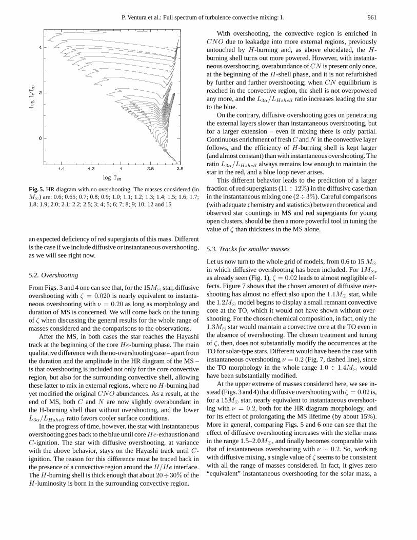
Fig. 5. HR diagram with no overshooting. The masses considered (inM�) are: 0.6; 0.65; 0.7; 0.8; 0.9; 1.0; 1.1; 1.2; 1.3; 1.4; 1.5; 1.6; 1.7;1.8; 1.9; 2.0; 2.1; 2.2; 2.5; 3; 4; 5; 6; 7; 8; 9; 10; 12 and 15

an expected deficiency of red supergiants of this mass. Differentis the case if we include diffusive or instantaneous overshooting,as we will see right now.

5.2. Overshooting

From Figs. 3 and 4 one can see that, for the 15M� star, diffusiveovershooting withζ = 0.020 is nearly equivalent to instanta-neous overshooting withν = 0.20 as long as morphology andduration of MS is concerned. We will come back on the tuningof ζ when discussing the general results for the whole range ofmasses considered and the comparisons to the observations.

After the MS, in both cases the star reaches the Hayashitrack at the beginning of the coreHe-burning phase. The mainqualitative difference with the no-overshooting case – apart fromthe duration and the amplitude in the HR diagram of the MS –is that overshooting is included not only for the core convectiveregion, but also for the surrounding convective shell, allowingthese latter to mix in external regions, where noH-burning hadyet modified the originalCNO abundances. As a result, at theend of MS, bothC andN are now slightly overabundant inthe H-burning shell than without overshooting, and the lowerL3α/LHshell ratio favors cooler surface conditions.

In the progress of time, however, the star with instantaneousovershooting goes back to the blue until coreHe-exhaustion andC-ignition. The star with diffusive overshooting, at variancewith the above behavior, stays on the Hayashi track untilC-ignition. The reason for this difference must be traced back inthe presence of a convective region around theH/He interface.TheH-burning shell is thick enough that about20÷30% of theH-luminosity is born in the surrounding convective region.

With overshooting, the convective region is enriched inCNO due to leakadge into more external regions, previouslyuntouched byH-burning and, as above elucidated, theH-burning shell turns out more powered. However, with instanta-neous overshooting, overabundance ofCN is present only once,at the beginning of theH-shell phase, and it is not refurbishedby further and further overshooting; whenCN equilibrium isreached in the convective region, the shell is not overpoweredany more, and theL3α/LHshell ratio increases leading the starto the blue.

On the contrary, diffusive overshooting goes on penetratingthe external layers slower than instantaneous overshooting, butfor a larger extension – even if mixing there is only partial.Continuous enrichment of freshC andN in the convective layerfollows, and the efficiency ofH-burning shell is kept larger(and almost constant) than with instantaneous overshooting. TheratioL3α/LHshell always remains low enough to maintain thestar in the red, and a blue loop never arises.

This different behavior leads to the prediction of a largerfraction of red supergiants (11÷12%) in the diffusive case thanin the instantaneous mixing one (2÷3%). Careful comparisons(with adequate chemistry and statistics) between theoretical andobserved star countings in MS and red supergiants for youngopen clusters, should be then a more powerful tool in tuning thevalue ofζ than thickness in the MS alone.

5.3. Tracks for smaller masses

Let us now turn to the whole grid of models, from 0.6 to 15M�in which diffusive overshooting has been included. For1M�,as already seen (Fig. 1),ζ = 0.02 leads to almost negligible ef-fects. Figure 7 shows that the chosen amount of diffusive over-shooting has almost no effect also upon the1.1M� star, whilethe1.2M� model begins to display a small remnant convectivecore at the TO, which it would not have shown without over-shooting. For the chosen chemical composition, in fact, only the1.3M� star would maintain a convective core at the TO even inthe absence of overshooting. The chosen treatment and tuningof ζ, then, does not substantially modify the occurrences at theTO for solar-type stars. Different would have been the case withinstantaneous overshootingν = 0.2 (Fig. 7, dashed line), sincethe TO morphology in the whole range1.0 ÷ 1.4M� wouldhave been substantially modified.

At the upper extreme of masses considered here, we see in-stead (Figs. 3 and 4) that diffusive overshooting withζ = 0.02 is,for a15M� star, nearly equivalent to instantaneous overshoot-ing with ν = 0.2, both for the HR diagram morphology, andfor its effect of prolongating the MS lifetime (by about 15%).More in general, comparing Figs. 5 and 6 one can see that theeffect of diffusive overshooting increases with the stellar massin the range 1.5–2.0M�, and finally becomes comparable withthat of instantaneous overshooting withν ∼ 0.2. So, workingwith diffusive mixing, a single value ofζ seems to be consistentwith all the range of masses considered. In fact, it gives zero“equivalent” instantaneous overshooting for the solar mass, a


Fig. 6. HR diagram with diffusive overshooting,ζ = 0.02

slowly increasing effect for larger masses up to∼ 2M�, afterwhich it mimicks∼ 0.2Hp of instantaneous overshooting.

The reason for this smooth growth of “equivalent” over-shooting is mainly in thenon-localflavor introduced in the mod-els thanks tofthick in Eq. (4). As already quoted in Sect. 4.2, forlow mass stars like the Sun the size of the initial convective coreis quite small, much less than the value ofHp at the convec-tive boundary, and also the value offthick is correspondinglylow. This gives rise to a stiff velocity profile in the overshootingregion, which in turn leads to very little mixing and fast fad-ing of the core. For larger masses, the size of the core growsand so alsofthick, until saturation or quite so. Including somenon-locality, even in a rough approximation, in the modelingof turbulent convection always gives more straightforward andphysically realistic results, as already found for the superadi-abatic temperature gradient thanks to the introduction ofz asconvective scale length (Sect. 2.1). In the present case, we do nothave to select different mass ranges with different tunings of theinstantaneous overshooting parameterν; we can simply applythe same tuning forζ to any mass range as a first, reasonableapproximation.

6. Comparisons with previous evolutionary tracks

Among the several authors having provided in the past evolu-tionary sets of intermediate mass stars, the more recent onesare Chin & Stothers 1990, 1991; Schaller et al. (1992), Bro-cato & Castellani (1993), Schaerer et al. (1993), Mowlavi etal. (1994), Deng et al. (1996a,b). It is worth comparing ourresults with previous models computed with analogously up-dated micro-physical inputs, although an FST coupled-diffusivemixing and overshooting has not yet used by other authors.We then excluded from our comparisons the models by Chin& Stothers (1990, 1991) and by Brocato & Castellani (1993),

Fig. 7. Blow-up of the theoretical HR diagram for stars in the range1.1÷1.3M�, with and without diffusive overshooting. The differencebetween the two cases is that, withζ = 0.02, also the star of1.2M�maintains a small convective core at the turn-off, while in the formercase the same occurrence was found for1.3M�

since they adopted radiative opacities quite different from theupdated OPAL ones present in our models. More reasonable arethe comparisons with the results by Schaller et al. (1992, here-after SSMM), Mowlavi & Forestini (1994, hereafter MF), Denget al. (1996a,b,, hereafter DBC), since their input micro-physicis much closer to the one inATON 2.0 code. Of course, all theabove quoted authors used the Mixing Length Theory (even ifDBC worked out some corrections to the plain MLT) to dealwith convection. In Fig. 8 we show the variation with mass ofthe hydrogen burning times computed by ourselves and by theauthors mentioned above.

Before performing more detailed comparisons, we evaluatedfirst–approximation transformations of luminosity andTeff toslightly different chemistries, to better compare our results tothe ones obtained in Zero Age Main Sequence (ZAMS) withdifferent (Y, Z) values. They turned out:

δ log L/L� ' 1.79δY − 3.83δZ

δ log Teff ' 0.42δY − 2.57δZ

First we considered the models by SSMM, for (Y , Z)=(0.30,0.020), in which instantaneous overshooting of0.2Hp is present.Given the chemistries, we must add to their ZAMS points thevaluesδ log L/L� ' −0.035 andδ log Teff ' −0.0032. TheZero Age Main Sequence locations turn out very similar; ourZAMS structures are in the average slightly more luminous andhotter, the maximum differences being however only∼ .05 inlog L/L� and∼ 0.015 in log Teff . This similiarity is not sur-prising, since the physical inputs are very close both in SSMMand in our models.


0 0.5 1

7

8

9

10

11

0 0.5 1

7

8

9

10

11

SSMMDBCIIMFDBCI

Fig. 8. Comparison of our results with those of other authors

This is not yet, however, a test on overshooting, which onlyaffects the width of the MS. For the range of mass1.5 ÷ 5M�,also the width is similar in the present models with diffusiveovershooting (ζ = 0.02) and in SSMM. The average discrep-ancy is again of0.01 ÷ 0.02 in log Teff . For larger masses(7÷15M�) the width of our MS band is slightly, sistematicallylarger (0.04÷0.05 in log Teff ). Closely related to the amplitudeof MS is also its duration. In Fig. 8 we see that the lifetimes ofstars in coreH-burning phase in SSMM models are very similarto ours up to∼ 4M�, while SSMM get fasterH-exhaustion forlarger masses. At15M�, our lifetime in MS is∼ 9% longerthan for SSMM. As already seen, half of the difference is dueto our coupled-diffusion (Sect. 4.1) evolutionary scheme; theremaining4 ÷ 5% can be attributed to the non exact identity ofdiffusive and instantaneous overshooting, and to residual differ-ences in the physical and chemical inputs between the two setsof models.

Analogous results are found when comparing our modelswith those by MF, where instantaneous mixing and overshootingwith ν =0.20 are applied to models withM =2.5, 5, 10, 15M�, and (Y, Z)=(.275,.020). Small differences in lifetime ofH-burning (2 ÷ 5%) are found; the width of our MS is slightlysmaller than in MF by0.002÷0.007 (that is: almost negligible)in log Teff for the whole range of masses considered. Also theMS lifetimes are very close in both cases.

Interesting comparison can be made also with the DBC mod-els, since they adopt a diffusive algorithm to deal with over-shooting. For completeness, in Fig. 8 we also plot their mod-els obtained with a classical instantaneous mixing scheme. Themost outstanding result when comparing models obtained withdiffusive overshooting is the similarity between our times ofhydrogen burning with theirs over the whole range of massesspanned, our lifetimes being larger than their at15M� just by3 ÷ 4%, that is: the difference due to coupled-diffusion evo-

Table 4.Lifetime H-burning (in unit of106 yr) DBC1 stands for clas-sical mixing, while DBC2 for diffusive process

MM� tH(noov) tH(ov) tH(PI) tH(MF ) tH(DBC1) tH(DBC2)

0.6 66630.0 66651.5 - - - -0.65 50498.7 50512.6 - - - -0.7 38598.5 38623.4 - - - -0.8 23683.2 23684.3 25027.9 - - -0.9 15079.6 15045.6 15500.3 - - -1.0 9728.1 9685.2 9961.7 - - -1.1 6517.3 6496.2 - - - -1.2 4343.3 4388.8 - - - -1.3 3381.5 3817.4 - - - -1.4 2623.3 3055.9 - - - -1.5 2097.0 2468.2 2694.7 - - -1.7 1455.7 1713.8 1827.3 - - -2.0 925.03 1086.1 1115.9 - - -2.5 506.92 580.79 584.92 628 - -3.0 312.33 355.43 352.50 - - -4.0 149.35 170.96 164.73 - - -5.0 87.620 99.849 94.459 101.6 81.58 101.276.0 57.925 65.961 - - - 67.997.0 41.727 47.825 43.188 - 40.42 48.728.0 31.851 36.453 - - - -9.0 24.832 29.029 26.389 - 24.93 28.5510.0 20.863 23.959 - 23.67 - -12.0 15.386 17.989 16.018 - 12.21 17.1715.0 11.177 12.758 11.584 12.74 10.90 12.31

lutionary scheme. We conclude then that, apart for this latterfeature, the two overshooting algorithms used by DBC and byourselves have almost the same effect, at least when dealingwith main sequence stars of intermediate mass.

In the end, we want to stress what we already claimed, thatis:

-this first test confirms that, on quantitative grounds, diffu-sive overshooting withζ = 0.02 gives results consistent withthose obtained with instantaneous overshooting,ν = 0.2, with-out having to care of setting overshooting to zero atM <1.5 ÷ 2.0M� and having a more physically sound descriptionof the occurrences at the convective boundaries;

-the differences due to the use of the coupled-diffusionscheme instead of the instantaneous mixing one are of the samemagnitude of other differences due to physical and chemicalinputs; they must be accounted for in updated generations ofstellar models.

7. Isochrones and the age of young open clusters

We have computed isochrones from our models and have trans-formed them into the observationalMv–B−V plane. The tracksare transformed by adopting Kurucz & Castelli (1996, privatecommunication) model atmosphere relations betweenTeff andB−V . The semiempirical transformations by Flower (1996) aresimilar, but provide bluer main sequence colors -by∼ 0.05 mag


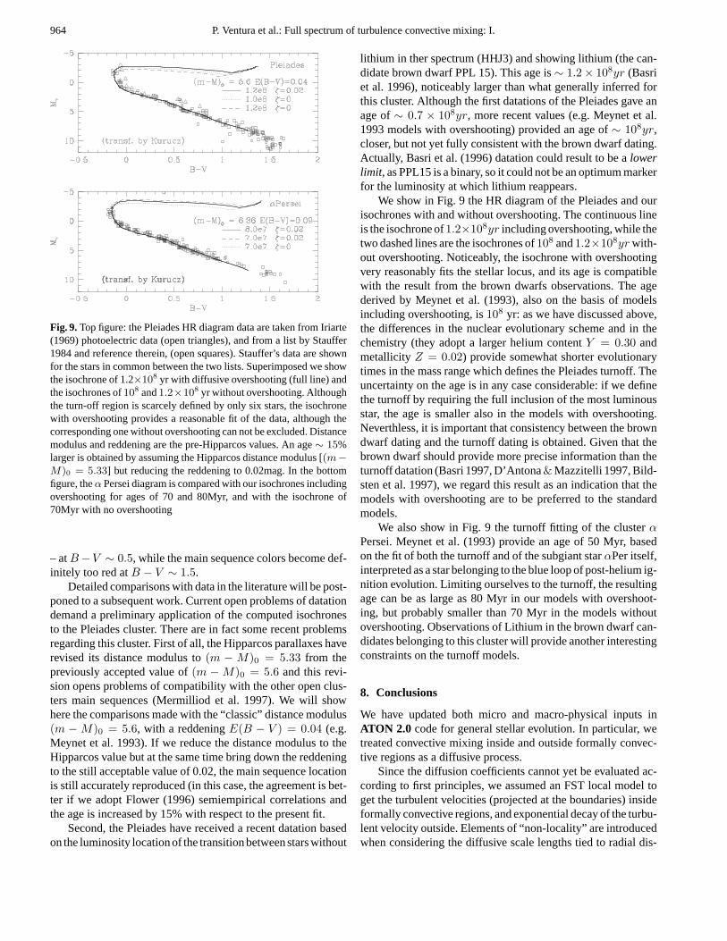
Fig. 9.Top figure: the Pleiades HR diagram data are taken from Iriarte(1969) photoelectric data (open triangles), and from a list by Stauffer1984 and reference therein, (open squares). Stauffer’s data are shownfor the stars in common between the two lists. Superimposed we showthe isochrone of 1.2×108 yr with diffusive overshooting (full line) andthe isochrones of108 and1.2×108 yr without overshooting. Althoughthe turn-off region is scarcely defined by only six stars, the isochronewith overshooting provides a reasonable fit of the data, although thecorresponding one without overshooting can not be excluded. Distancemodulus and reddening are the pre-Hipparcos values. An age∼ 15%larger is obtained by assuming the Hipparcos distance modulus [(m−M)0 = 5.33] but reducing the reddening to 0.02mag. In the bottomfigure, theα Persei diagram is compared with our isochrones includingovershooting for ages of 70 and 80Myr, and with the isochrone of70Myr with no overshooting

– atB −V ∼ 0.5, while the main sequence colors become def-initely too red atB − V ∼ 1.5.

Detailed comparisons with data in the literature will be post-poned to a subsequent work. Current open problems of datationdemand a preliminary application of the computed isochronesto the Pleiades cluster. There are in fact some recent problemsregarding this cluster. First of all, the Hipparcos parallaxes haverevised its distance modulus to(m − M)0 = 5.33 from thepreviously accepted value of(m − M)0 = 5.6 and this revi-sion opens problems of compatibility with the other open clus-ters main sequences (Mermilliod et al. 1997). We will showhere the comparisons made with the “classic” distance modulus(m − M)0 = 5.6, with a reddeningE(B − V ) = 0.04 (e.g.Meynet et al. 1993). If we reduce the distance modulus to theHipparcos value but at the same time bring down the reddeningto the still acceptable value of 0.02, the main sequence locationis still accurately reproduced (in this case, the agreement is bet-ter if we adopt Flower (1996) semiempirical correlations andthe age is increased by 15% with respect to the present fit.

Second, the Pleiades have received a recent datation basedon the luminosity location of the transition between stars without

lithium in ther spectrum (HHJ3) and showing lithium (the can-didate brown dwarf PPL 15). This age is∼ 1.2 × 108yr (Basriet al. 1996), noticeably larger than what generally inferred forthis cluster. Although the first datations of the Pleiades gave anage of∼ 0.7 × 108yr, more recent values (e.g. Meynet et al.1993 models with overshooting) provided an age of∼ 108yr,closer, but not yet fully consistent with the brown dwarf dating.Actually, Basri et al. (1996) datation could result to be alowerlimit, as PPL15 is a binary, so it could not be an optimum markerfor the luminosity at which lithium reappears.

We show in Fig. 9 the HR diagram of the Pleiades and ourisochrones with and without overshooting. The continuous lineis the isochrone of1.2×108yr including overshooting, while thetwo dashed lines are the isochrones of108 and1.2×108yr with-out overshooting. Noticeably, the isochrone with overshootingvery reasonably fits the stellar locus, and its age is compatiblewith the result from the brown dwarfs observations. The agederived by Meynet et al. (1993), also on the basis of modelsincluding overshooting, is108 yr: as we have discussed above,the differences in the nuclear evolutionary scheme and in thechemistry (they adopt a larger helium contentY = 0.30 andmetallicity Z = 0.02) provide somewhat shorter evolutionarytimes in the mass range which defines the Pleiades turnoff. Theuncertainty on the age is in any case considerable: if we definethe turnoff by requiring the full inclusion of the most luminousstar, the age is smaller also in the models with overshooting.Neverthless, it is important that consistency between the browndwarf dating and the turnoff dating is obtained. Given that thebrown dwarf should provide more precise information than theturnoff datation (Basri 1997, D’Antona& Mazzitelli 1997, Bild-sten et al. 1997), we regard this result as an indication that themodels with overshooting are to be preferred to the standardmodels.

We also show in Fig. 9 the turnoff fitting of the clusterαPersei. Meynet et al. (1993) provide an age of 50 Myr, basedon the fit of both the turnoff and of the subgiant starαPer itself,interpreted as a star belonging to the blue loop of post-helium ig-nition evolution. Limiting ourselves to the turnoff, the resultingage can be as large as 80 Myr in our models with overshoot-ing, but probably smaller than 70 Myr in the models withoutovershooting. Observations of Lithium in the brown dwarf can-didates belonging to this cluster will provide another interestingconstraints on the turnoff models.

8. Conclusions

We have updated both micro and macro-physical inputs inATON 2.0 code for general stellar evolution. In particular, wetreated convective mixing inside and outside formally convec-tive regions as a diffusive process.

Since the diffusion coefficients cannot yet be evaluated ac-cording to first principles, we assumed an FST local model toget the turbulent velocities (projected at the boundaries) insideformally convective regions, and exponential decay of the turbu-lent velocity outside. Elements of “non-locality” are introducedwhen considering the diffusive scale lengths tied to radial dis-


tances from convective boundaries. Full coupling between nu-clear chemical evolution and turbulent mixing is assumed.

One relevant result is that the CNO equilibria in the con-vective cores of large mass main sequence stars do require suchcoupling in the models computation. Instantaneous or diffusivemixing decoupled from nuclear evolution leads to discrepancesin the evaluation of evolutionary times.

As for overshooting, we chose a conservative value for thefree parameter of diffusionζ such that it should have a negligi-ble effect on the early convective core of the Sun, and mimickthe effect of an instantaneous overshooting of∼ 0.20Hp forintermediate to large mass stars. This tuning is obviously pre-liminary, and requires further tests and comparisons not only inmain sequence but also in other evolutionary phases. Next pa-pers on the subject will follow, with application of the presentdiffusive scheme mainly to horizontal branch and to thermallypulsating stars.

We also compared our results with the more recent ones inthe literature, finding satisfactory agreement so far as the differ-ent chemical compositions and mixing schemes could allow.

9. Appendix: the ATON 2.0 code

9.1. Generalities

In this appendix, we provide a synthetic but exhaustive descrip-tion of the numerical inputs of the codeATON 2.0, to comple-ment the elucidation in Sects. 2 and 3 of the main macro/micro-physical inputs. The choice of fully document the code will alsohelp us, in the future, to avoid useless debates about results ob-tained from codes having different and/or not fully documentedinputs.

ATON 2.0 describes spherically symmetric structures in hy-drostatic equilibrium. It has been conceived to follow the evo-lution of stellar objects from early pre-main sequence phasesprior to D-ignition, down to final brown or white dwarf cooling(apart from dynamical phases like full degenerate He-ignition)or to the onset and early developement of12C +12 C reactions.The ignition of16O +16 O and the following (pre-supernova)phases are not accounted for. In future papers, we will alwaysrefer to anATON N.M version of the code, whereN will keeptrack of the major macro-physical updates (e.g. rotation, nongrey atmospheres etc), andM of the micro-physical ones (ther-modynamics, opacities etc). In the same spirit above discussed,any change of release will be fully documented.

9.2. The numerical structure

The internal structure is integrated via the usual Newton–Raphson relaxation (Henyey) method, from the center to thebase of the optical atmosphere (τ = 2/3). The independent vari-able is the mass; the dependent ones are: 1) radius, 2) total lumi-nosity, 3) total pressure and 4) temperature. To avoid numericalprecision problems close to the surface, where∆M/Mtot canbe∼ 10−12 ÷ 10−18, the code rezones and performs numeri-cal derivatives directly on the∆M vector, and the local valueof mass at each grid point is obtained as a summation of∆M

from the center. This procedure, as opposed to the traditionalone of computing grids of subatmospheres – with pressure asindependent variable – down to a given fraction ofMtot, allowsstraightforward evaluation of the gravothermal energy genera-tion rate up to the stellar surface, especially when mass loss (e.g.in contact binaries) plays a dominant role on the structure.

Given theith grid point, and thejth dependent variableqj(i),the correctionsδqj(i) can be found from the solution of thesystem (in Einstein notation):

∂EQ(1 ÷ 4)∂qj(i)

δqj(i) +∂EQ(1 ÷ 4)∂qj(i + 1)

δqj(i + 1) + β(1 ÷ 4)

= 0 , (A.1)

whereEqs. (1÷4) are the four canonical differential equations,andβ(1 ÷ 4) are the residuals. Since only two boundary con-ditions are known at the center, the values ofδqj(i) cannot befound until the surface is reached. We then compute at each gridpoint the matrix elementsµ andν, and the vector elementsεsuch that

δqj(i) = µkj (i)δqk(i) + νk

j (i)δqk(i + 1) + εj(i) (A.2)

The only non-vanishing coefficients are:µ3

1; µ41; µ3

2; µ42; ν3

3 ; ν43 ; ν3

4 ; ν44 ; εj

Once reached the surface (base of the optical atmosphere)the system is closed by the integration of three optical atmo-spheres, with (L,R), (L+δL,R), (L,R+δR). Backward applica-tion of Eq. (A2) allows the evaluation of all theδqj(i)’s. Notethat, with the above choice,ν3

3 andν44 ∼ 1, and also all the

other coefficients do not depart from unity for too many ordersof magnitude, avoiding round-off and truncation errors. Also,during the iterations to convergency, the∆qj values are updatedas

∆qj(new)(i) = ∆qj(old)(i) + δqj(i + 1) − δqj(i)

and new values of∆qj are differentially computed only afterconvergency.

9.3. Internal zoning, time steps and nuclear evolution

Internal zoning of the structure is reassessed at each physicaltimestep, with particular care in the central and surface regions,in the vicinities of convective boundaries and H or He-burningshells, and close to the superadiabaticity peak. Tipically, pre-main sequence and main sequence structures are resolved in800 ÷ 1200 grid points; red giants in1200 ÷ 1500 grid points,∼ 400 of which in the thin H-burning shell; horizontal branchstructures contain1500 ÷ 2000 grid points and, during thermalpulses, up to∼ 3000 grid points are often reached.

The physical time step is evaluated according to experience,allowing maximum variations, both integral and local along thestructure, of several physical and chemical quantities. Amongthe integral quantities, total, CNO,3α and 12C +12 C lumi-nosities are considered; among the local ones, the four struc-tural quantities and the central chemical compositions. The fi-nal time step chosen is obviously the shortest one out of the∼


fifteen evaluated. For a solar-like star, evolution from pre-mainsequence to turn-off takes∼ 1000 physical time steps; He-flashis reached after15000 ÷ 20000 time steps (no shell projec-tion), in horizontal branch central He-exhaustion is reached in∼ 2000 ÷ 4000 time steps, and one fully developed thermalpulse cycle, from peak to peak takes∼ 3000÷5000 time steps.

So far we spoke of “physical” time steps. For the purposesof chemical evolution only, each physical time step is furtherdivided into at least 10 “chemical” time steps. Any mechanismleading to a variation of chemical composition, such as nuclearevolution, gravitational settling and convective mixing, is re-peatedly applied for the number of chemical time steps up tothe reaching of the physical time step, projecting pressure andtemperature to get also projected nuclear reaction rates. In thisway, the evolution up to the He-flash can require up to2 × 105

chemical time steps, and the advancement of an H-burning shellfrom step to step is only a tiny fraction of its thickness.

As for the chemical evolution, we adopt the implicit schemeby Arnett & Truran (1969). It can be assumed equivalent to afirst order Runge-Kutta, since it accounts for both the initial andthe final chemical composition in the evaluation of the reactionrates. The integration error is then proportional to(∆X)2. Thealternative approach to compute the rates for the initial abun-dances only can be instead assimilated to a zero order Runge-Kutta, and the integration error would be proportional to(∆X),being then much larger. To restore better integration precision inthis latter case, it is customary to divide eachphysicaltimestepin a large number ofchemicaltimesteps, decreasing in this way(∆X) for each step. Also in codeATON 2.0, however, thephysical timestep is divided in several chemical ones, as abovementioned, leading to almost vanishing numerical errors in thenuclear evolution integration.

If instantaneous mixing of convective regions is adopted(not recommended, since diffusive mixing is more physicallysound), the average chemistry and reaction rates over all theregion are evaluated, and the linearization procedure applied tothe whole region as a single grid point. The very small variationsof chemistry with time obtained in this way ensure enormouslybetter numerical precision of integration than the alternativeprocedure of locally evaluating the new chemistries and thenmixing.

9.4. Diffusive mixing

In the case of diffusive mixing, we must solve Eq. (1) to getthe new chemical abundancesY n+1

a,i at timetn+1 for each el-ementa at each mesh pointi. Nuclear evolution and mixingare strictly interwined, so that their simultaneous resolution isinvoked. We adopted a network of 22 nuclear reactions for 14elements (Sect. 3.3).

The equation describing the rate of change of abundance forthe nucleusa, having number densityNa, is:

∂Ya

∂t=

1r2ρ

∂

∂r

(r2ρD

∂a

∂r

)±∑l≥k

YlYk [lk]

whereYa = Na/ρNA (NA = Avogadro’s number).

Using a finite difference method based on a two-time leveland three-point scheme, Eq. (A1) can be approximated by

AaY n+1a,i

= AaY na,i + ∆t

{∑[p, q]n+1/2

×[Y np,iY

nq,i + (Y n+1

p,i − Y np,i)Y

nq,i + (Y n+1

q,i − Y nq,i)Y

np,i]

−∑

[a, j]n+1/2[Y na,iY

nj,i + (Y n+1

a,i − Y nj,i)Y

nj,i

+(Y n+1j,i − Y n

a,i)Yna,i] +

2Aa

mi+1 − mi−1

×[σ

n+1/2i+1/2

Y n+1a,i+1 − Y n+1

a,i

mi+1 − mi− σ

n+1/2i−1/2

Y n+1a,i+1 − Y n+1

a,i−1

mi − mi−1

]}(A2.a)

Y n+1a,base = Ya,base+1 (A2.b)

Y n+1a,surf = Ya,surf−1 (A2.c)

whereσn+1i±1/2 = 16π2r4ρ2D is computed at half-integer grid

points. The boundary conditions have the meaning of no con-vective flux at the boundaries of convective (plus overshooting– if any) region, since no mass exchange with the non turbulentregions of the star is allowed.

Equation (A2.a) can be rewritten as

∆t · B(a)j = −αa,iγiYn+1a,i−1 − αa,iβiY

n+1a,i+1

+∆t ·∑

k

A(a, k)iYn+1k,i + αa,i (γj + βi)Y n+1

a,i (A3)

whereαa,i = 2∆tAa

mi+1−mi−1; βi =

σn+1/2i+1/2

mi+1−mi; γi =

σn+1/2i−1/2

mi−mi−1

where A(a,k) stands for the coefficients of theY n+1k,i terms and

B(a) stands for terms relative to time steptn. Note that theabundance of each element at a given grid point is coupledto the abundances of all the other elements at the same gridpoint, and to its own abundance at adjacent grid points. Sincethe two boundary conditions are met at the base and at the topof convection, the problem can not be explicitly solved until thewhole convective region is addressed.

We now provide a description of the numerical methodadopted to solve the system (A3, A2.a, A2.b).

For each convective region ofTot grid points, we should inprinciple compute, store and invert a(14·Tot, 14·Tot)matrix. Acareful analysis of Eq. (A3) shows however that the storage of a(42, 14·Tot) matrix is sufficient, since only the matrix elementsclose to the diagonal are nonzero. Our problem has been reducedto solve a systemA · y = B, whereA = (42, 14 · Tot), whileB = (14 · Tot).

Were A a square matrix, it would be possible to save com-puter time by applying the usual L–U (lower-upper) triangulardecomposition (Crout’s algorithm) such thatL · U = A. Itera-tively evaluating L and U, and recalling that

A · y = (L · U) · y = L · (U · y) = Bone would get the vector x such thatL · x = B, and finally

the vector y so thatU · y = x.We adapted Crout’s algorithm to our matrix. Beinga andj

two generic chemical elements and i the spatial grid point (from


the base of the convective regioni = ibot, to the topi = itop)the algorithms used to determine L and U are as follows:

i = ibot ; 1 ≤ a ≤ NEC

U(NEC + a, a, i) = A(NEC + a, a, i)

L(a, a, i + 1) = A(a, a, i + 1)/U(NEC + a, a, i)

ibot ≤ i < itop ; 1 ≤ a ≤ NEC

U(2NEC + a, a, i) = A(2NEC + a, a, i)

ibot < i ≤ itop − 1 ; 1 ≤ a < NEC; a + 1 ≤ j ≤ NEC

U(2NEC + a, j, i)

= −NEC∑

j=a+1

j−1∑m=a

U(2NEC + a, m, i)L(NEC + m, j, i)

ibot ≤ i < itop ; 1 ≤ a ≤ NEC; 1 ≤ j ≤ a

U(NEC + a, j, i + 1) = A(NEC + a, j, i + 1)

−j−1∑m=1

L(NEC + m, j, i + 1)U(NEC + a, m, i + 1)

−NEC∑m=a

L(m, j, i + 1)U(2NEC + a, m, i)

ibot ≤ i < itop ; 1 ≤ a ≤ NEC; a + 1 ≤ j ≤ NEC

L (NEC + a, j, i + 1) =A(NEC + a, j, i + 1)U(NEC + a, a, i + 1)

−∑a−1

m=1 L(NEC + m, j, i + 1)U(NEC + a, m, i + 1)U(NEC + a, a, i + 1)

−∑NEC

m=j L(m, j, i + 1)U(2NEC + a, m, i)U(NEC + a, a, i + 1)

ibot ≤ i < itop − 1 ; 1 < a ≤ NEC; 1 ≤ j < a

L(a, j, i + 2)

= −∑a−1

m=j L(m, j, i + 2)U(NEC + a, m, i + 1)U(NEC + a, a, i + 1)

(A3)

i0 ≤ i < isurf − 1 ; 1 ≤ a ≤ NEC

L(a, a, i + 2) =A(a, a, i + 2)

U(NEC + a, a, i + 1)

Since the terms of the L and U matrices do not occupy thesame location, and since each element of matrix A is used justonce to evaluate the corrisponding ones of matrices L and U,these new elements can be stored in matrice A.

The iterative procedure to evaluate the vector x is:

ibot < i ≤ itop ; 1 ≤ a ≤ NEC

X(a, i) = B(a, i) −NEC∑m=a

A(m, a, i)X(m, i − 1)

−a−1∑m=1

A(NEC + m, a, i)Y (m, i)

Finally the new abundancesY (a, i) for each element can beobtained from the following:

i = itop ; a = NEC

Y (a, i) =X(a, i)

A(2a, a, i)

i = itop ; NEC < a ≤ 1

Y (a, i) =

[X(a, i) −∑NEC

m=a+1 A(NEC + m, a, i)X(m, i)]

A(NEC + a, a, i)

itop < i < ibot ; NEC ≤ a ≤ 1

Y (a, i) =X(a, i)

A(NEC + a, a, i)

−∑a

m=1 A(2NEC + m, a, i)X(m, i + 1)A(NEC + a, a, i)

−∑NEC

m=a+1 A(NEC + m, a, i)X(m, i)A(NEC + a, a, i)

i = itop ; a = NEC

Y (a, i) = −A(2NEC + a, a, i)X(a, i + 1)A(NEC + a, a, i)

To further reduce storage allocation, it is again possible tostore each new element Y(a,i) in the corrisponding location ofX(a,i).

References

Alcock C., Illarionov A. 1980, ApJ 235, 541Alexander D.R., Ferguson J.W. 1994, ApJ 437, 879Aller L.H., Chapman S. 1960, ApJ 132, 461Arnett W.D., Truran J.W. 1969, ApJ 157, 359Bahcall J.N., Pinsonneault M.H. 1992, Rev. Mod. Phys. 64, 885Basri G. 1997 in “Cool Stars in Clusters ans Associations” eds. R.

Pallavicini & G. Micela, Mem.S.A.It., 68, n.4Basri G., Marcy G., Graham J.R. 1996, ApJ 458, 600Basu S., Antia H.M., 1997, MNRAS 287, 189Bildsten L., Brown E.F., Matzener C.D., Ushomirski G. 1997, ApJ 482,

442Brocato E., Castellani V. 1993, ApJ 410, 99Canuto V.M. 1992, ApJ 392, 218Canuto V.M., Mazzitelli I. 1992, ApJ 389, 724Canuto V.M., Goldman I., Mazzitelli I. 1996, ApJ 473, 550Caughlan G.R., Fowler W.A. 1988, Atomic Data Nucl. Tab. 40, 283Chin C.W., Stothers R.B. 1990, ApJS 73, 821Chin C.W., Stothers R.B. 1991, ApJS 77, 299Chiosi C. 1997, in “Stellar Astrophysics for the Local Group: a first

step to the Universe”, eds. A.J. Aparicio & A. Herrero, CambridgeUniversity Press, in press


Christensen - Dalsgaard J., Gough D.O., Thompson M.J. 1991, ApJ,378, 413

Cloutman L.D., Eoll J.G. 1976, ApJ 206, 548D’Antona F., Mazzitelli I. 1997, in “Cool Stars in Clusters and Asso-

ciations”, eds. R. Pallavicini & G.Micela, Mem.S.A.It., 68, n.4Deng L., Bressan A., Chiosi C. 1996a, A&A 313, 145Deng L., Bressan A., Chiosi C. 1996b, A&A 313, 159Flower P.J., 1996, ApJ, 469, 335Fontaine G., Michaud G. 1979, in IAU Colloquium 53,White dwarfs

and variable degenerate stars, ed. H. M. Van Horn and V. Weide-mann (Rochester, N.Y.: University of Rochester), 192

Fontaine G., Graboske H.C. Jr., Van Horn H.M. 1977, ApJ Suppl. 35n. 3, 293

Graboske H.C., De Witt H.E., Grossman A.S., Cooper M.S. 1973, ApJ181, 457

Grevesse N., 1984, Phys. Scr., T8, 49Grevesse N., Noels A. 1993, inOrigin and evolution of the Elements,

ed. N. Prantzos, E. Vangioni - Flam, and M. Casse (Cambridge:Cambridge University Press), 14

Grossman S.A. 1996, MNRAS 279, 305Iben I., MacDonald J. 1985, ApJ 296, 540Iriarte A. 1969, Boll. Obs. Tonantzintla y Tacubaya 5, 89Itoh N., Kohyama, Y. 1993, ApJ 404,268Itoh N., Mutoh H., Hikita A., Kohyama Y. 1992, ApJ 395, 622Lamb H., 1932, Hydrodynamics (Cambridge: Cambridge University

press)Kurucz R.L. 1993, CD-ROM 13 and CD-ROM 14Maeder A. 1990, A&AS 84, 139

Maeder A., Meynet G. 1987, A&A 182, 243Maeder A., Meynet G. 1991, A&AS 89, 451Magni G., Mazzitelli I. 1979, A&A 72, 134Mermilliod J.C., Turon C., Robichon N., Arenou F., Lebreton Y., 1997,

in “Hipparcos Venice ’97”, ESA SP-402, p.643Meynet G., Mermilliod J.C., Maeder A., 1993, A&AS 98, 477Mihalas D., Dappen W., Hummer D.G. 1988, ApJ 331, 815Mowlavi N., Forestini M. 1994, A&A 282, 843Muchmore D. 1984, ApJ, 278, 769Paquette C., Pelletier C., Fontaine G., Michaud G. 1986, ApJS 61, 1977Prandtl L. 1925, Zs. Angew. Math. Mech. 5, 136Profitt C.R., Michaud G. 1991, ApJ, 371, 584Rogers F.J., Iglesias C.A. 1993, ApJ 412, 572Rogers F.J., Swenson F.J., Iglesias C.A. 1996, ApJ 456, 902Roxburgh W. 1978, A&A 65, 281Sackmann J., Boothroyd A.I. 1995, Mem. Soc. Astr. It. 66, n.2, 403Salasnich B., Bressan A., Chiosi C. 1997, A&A, submittedSaumon D. 1994, inThe equation of state in Astrophysics, ed. G.

Chabrier and E. Shatzmann (Cambridge: Cambridge UniversityPress), 306

Saumon D., Chabrier G., Van Horn H.M., 1995, ApJS 99, 713Schaerer D., Meynet G., Maeder A., Schaller G. 1993, A&AS 98, 523Schaller G., Schaerer D., Meynet G., Maeder A. 1992, A&AS 96, 269Shaviv G., Salpeter E.E. 1973, ApJ 184, 191Stauffer J. 1984, ApJ 280, 189Stothers R.B., Chin C.W. 1992, ApJ 390, 136Vitense E., 1953, Zs. Ap. 32, 135Xiong D.R. 1985, A&A 150, 133

astron. astrophys. 334, 953–968 (1998) astronomy …aa.springer.de/papers/8334003/2300953.pdf3...

Documents