Astronomy 271B Lecture Notes, Spring 2016

c©Edward L. Wright, 2016

This is a course about the Fundamentals of Astrophysics: in particular electromagnetic

radiation. As astronomers we are limited to observing what happens in the Universe – we are

not able to reach out and touch something. Our observations are almost entirely done using

electromagnetic radiation. There are a very few exceptions: meteorites, charged cosmic rays

and neutrinos. Now that advanced LIGO has seen sources, we must add gravitational waves

to the list of observed radiation. But almost everything we know about the Universe comes

from light and non-visible EM radiation that reaches the Solar system.

I will try to get these LaTeX’d notes out in a timely fashion. They will not include all

the diagrams that I draw on the board, so you still need to take notes during class, but they

should help you remember what went on and also get the equations right.

A NOTE ABOUT UNITS: In this course we will use electrostatic cgs units because

most astrophysicists use them. Those of you who studied E&M in MKS units will suffer

the slings and arrows of outrageous unit conversion, but can probably fix a toaster. Just

remember that 1 picofarad is about 1 cm and that 1 gauss (that’s 10−4 Tesla) is the same

as 1 statvolt/cm which is 300 V/cm. All the best E&M books use cgs units: Purcell’s E&M

in the Berkeley Physics course, and Jackson in early editions.

The electrostatic force between two charges is F = k1q1q2/r2. The magnetic force

between two wires separated by distance r and carrying currents I1 and I2 per unit length λ

is dF/dλ = 2k2I1I2/r. Note that the speed of light is always given by c2 = k1/k2, the ratio

of electrostatic to magnetic force strengths. For MKS units k2 = 10−7 and thus k1 = 10−7c2,

while for electrostatic cgs units k1 = 1 and k2 = c−2. In the electrostatic cgs system ǫ = 1/4π

and µ = 4π/c2. The electrostatic cgs unit for charge is the electrostatic unit or esu, and 1

Coulomb is 2.99792458× 109 esu. That ratio is exactly c/10 cm/sec, and since the potential

energy is U = qV , the unit of electric potential in the cgs system is 299.792458 Volts which is

known as a statvolt. The unit of the electric field is statvolt/cm which is exactly the same as

the unit for the magnetic field which is the gauss. This fortunate coincidence arises because

the Lorentz force law, which is

F = q( ~E + ~v × ~B) (1)

in MKS units, is changed to

F = q( ~E + ~β × ~B) with β = v/c (2)

in cgs units, so ~E and ~B have the same units. Since we will be combining ~E and ~B into a single

electromagnetic field tensor Fµν it is very useful that ~E and ~B have the same units. The unit

for capacitance is esu/statvolt which is the centimeter so 1 Farad is (2.99792458)2×1011 cm.

Hence 1 cm is 1.1 pF. Since the RC time constant is still in seconds, (2.99792458)2 × 1011

Ohms is 1 sec/cm.

Since the resistance is given by R = ρL/A where ρ is the resistivity, L is the length and

A is the area, the units for the resistivity ρ are seconds. This is approximately the order

of magnitude for the length of time needed to discharge a spherical charge separation by

electrical conduction. For elongated objects like needles the discharge time is much longer

than the resistivity. To return to the toaster, the resistivity of nichrome is 110 × 10−8

Ohm-meters in MKS, or 110 µΩ-cm in the mixed units normally used. Since 1 Ohm is

1.1 × 10−12 sec/cm, the resistivity of nichrome is 1.2 × 10−16 sec. The discharge time is

significant for wavelengths λ ≈ 2πρc ≈ 0.2 µm for solid spheres and much longer wavelengths

for needle-shaped or porous dust grains.

1. Dust Absorption in the ISM

not in R&L

Typically in the ISM 1% of the mass is in dust. The heavy elements (C to U) make up

about 2% of the mass of the gas currently, but CO forms until one runs out of C or O, and

CO stays gaseous down to very low temperatures.

The “typical” dust grain has a radius a of about 0.1 µm = 10−5 cm. This value

is probably more set by λ/2π where λ is the wavelength of the light used to study the

dust. Because the dust grains are small, there is more absorption and scattering for short

wavelengths of light than for longer wavelengths. The sum of absorption and scattering is

known as extinction. The extinction vs. wavelength is denoted be Aλ. By comparing the

color of stars to the colors expected for the temperatures implies by their spectral types, the

color excess E can be determined. Most commonly one talks about E(B−V ) = AB−AV . If

the color excess, or reddening is known, one can determine the total extinction AV through

the ratio of total to selective extinction, R = AV /E(B−V ) ≈ 3.1. Note that if Aλ ∝ ν, then

R would be R = 0.55−1/(0.44−1 − 0.55−1) = 4 so the extinction curve is less steep than 1/λ

in the visible, but in the near infrared the extinction declines more rapidly than 1/λ with

increasing wavelength.

The typical dust grain has a mass mg = 4πa3ρ/3 ≈ 10−14 gm which corresponds to

about 1010 H atoms. Thus the number density of grains is about 10−12 of the number

density of hydrogen. In the typical ISM density nH = 1 cm−3, the distance between dust

grains is about 104 cm. Thus the ISM is very dilute and the dust grains act independently.

The dielectric constant of the ISM is given by ǫ = 1+4πχ where χ = P/E and P is the

2

dipole density. P is given by ngαgE where αg is the polarizability of the dust grain. Thus

ǫ = 1 + 4πngαg (3)

But what is the polarizability of a dust grain? It has the dimensions of (length)3 in cgs units.

For a perfectly conducting sphere, assume that there is a surface charge density σ = σ cos θ,

where θ is the angle between the incident E field and the point on the surface. This charge

density makes an E field at the center of the sphere given by

~Eind = z

∫

σ cos2 θdΩ =4πσ

3(4)

Thus, σ = 34πEext for the induced field to cancel the external field in the center of the sphere.

This surface charge density has a dipole moment given by

d =

∫

a cos θ(σ cos θa2)dΩ =4π

3a3σ = a3Eext (5)

so the polarizability of a conducting sphere is

αg = a3 (6)

For a dielectric sphere, the dipole density P inside the sphere is constant, as is the total

electric field E. The surface charge density is σ = P cos θ. Thus the induced field is

~Eind = −4π

3~P (7)

But the dipole density is given by

~P =(ǫg − 1) ~E

4π(8)

and the interior electric field is given by

~E = ~Eext + ~Eind (9)

Since all the electric fields are along the z axis and the direction of the induced field is

opposite to the applied field, we can find the magnitude of the induced field by solving

3

4πEind =

(ǫg − 1)

4π(Eext −Eind) (10)

so

Eind

(

3

4π+

(ǫg − 1)

4π

)

=(ǫg − 1)

4πEext (11)

and finally

Eind =ǫg − 1

ǫg + 2Eext (12)

3

The dipole moment is obviously

d =4π

3a3P = a3Eind =

ǫg − 1

ǫg + 2a3Eext (13)

and the polarizability of a dielectric sphere is

αg =ǫg − 1

ǫg + 2a3 (14)

For a conductor, ǫ = 1 − ω2p/ω

2 → −∞ so αg = a3 as found earlier. These formula are

derived using electrostatics (ω → 0) but are OK for λ >> a.

The imaginary part of the wavevector k = ω√ǫ/c is given by

ℑ(k) =ω

c(1 + 2πngαg) (15)

Now ℑ(k)×D gives the fractional reduction in the amplitude of |E|, so the reduction in the

power is twice this great. But this reduction in power is also given by

D × ng × σext = 2× ℑ(k)×D (16)

Thus the extinction cross section of dust grain is given by

σext =4πωℑ(αg)

c(17)

For a sphere,

σext = 4πa3ω

cℑ(

ǫg − 1

ǫg + 2

)

(18)

1.1. Scattering

The oscillating dipole moment of the dust grain emits power given by

P =2e2a2

3c3=

2d2ω4

3c3(19)

The Poynting flux times the scattering cross-section equals this power so

σscat =8π

3

(ω

c

)4

a6

∣

∣

∣

∣

ǫg − 1

ǫg + 2

∣

∣

∣

∣

2

(20)

Since the scattering goes down like ω4, the long wavelength extinction is dominated by

absorption.

4

The Kramers-Kronig relation for dust grains gives:

αDC =1

4π3

∫ ∞

0

σextdλ (21)

Note that σ can’t approach a constant greater than zero as λ → ∞ because that would

require an infinite DC polarizability. An extinction going like 1/λ is also ruler out, although

only logarithmicly.

To have a large σext at long wavelengths, one needs to have a large αDC . But for spheres,

αDC is proportional to the volume, and we can’t have a large volume without requiring too

much mass in the dust grains. To get around this limit, we need to find grains with a large

ratio αDC/V where V is the volume.

This is possible for conducting needles. Consider a needle with length L and diameter

D in an external electric field oriented parallel to the long axis of the needle. A linear charge

density λ(z) will be induced on the needle. Assume that λ(z) ∝ z with the origin at the

middle of the needle. The voltage of a linear charge density is given by V = 2λ ln r. Taking

the potential drop between r = D/2 and r = L/2 and setting this equal to the external

voltage Ez gives

λ(z) =Ez

2 ln(L/D)(22)

so the dipole moment is

d =

∫

λ(z)zdz =E

2 ln(L/D)

∫ L/2

−L/2

z2dz =L3

24 ln(L/D)E (23)

Thus the polarizability is proportional to the (longest dimension)3 instead of the volume.

For these formula to work it is necessary that the induced voltage cancel the applied volt-

age, which will happen if the grain is made out of a conducting material. Thus elongated

conducting dust grains can be very efficient long wavelength absorbers.

The absorption cross-section can be found by comparing the ohmic loss in the grain to

the Poynting flux. The ohmic loss is

Power =

∫

jEdV =

∫

σeE2dV (24)

where σe is the electrical conductivity of the material. Thus the absorption cross-section is

given by

σabs =4πσeV

c(25)

Note that in cgs units the electrical conductivity σe has the units sec−1 and is equal to the

usual value in mho/cm multiplied by 2.997924582 × 1011. For a typical amorphous carbon

σe = 100 mho/cm = 9× 1013 sec−1, the absorption cross-section is about 30, 000 cm2/cc or

5

approximately 104 cm2/gm of dust and 100 cm2/gm of total ISM. The visual extinction of 1

per kpc is 200 cm2/gm of total ISM, so conducting needles can have absorptions as high as

the visual extinction extending into the far-IR and sub-mm. For randomly oriented needles,

these values should be divided by 3 since only 1 of the 3 axes is along the long axis of the

needle.

This absorption cross-section assumes that current is flowing freely in the incident field,

but for long wavelengths the dipole moment gets established and the net field goes to zero,

and so does the absorbed power. The time constant for setting up the dipole moment can

be estimated by calculating the resistance and capacitance of the needle. The resistance

R is R = L/(πD2σe/4) and has units of sec/cm. The capacitance can be estimated from

the voltage across the needle, V = 4λ(L/2) ln(L/D), and the charge on one “plate” of the

needle, Q =∫ L/2

0λ(z)dz = (L/4)λ(L/2). Thus C = Q/V = L/(16 ln(L/D)) and has units

of cm. The time constant is

τ = RC =(L/D)2

4π ln(L/D)σe(26)

For L/D = 100 and σe = 1014 sec−1, this is τ = 1.7× 10−12 sec. Thus the cutoff at ωτ = 1

occurs at ω = 6× 1011, ν = 9× 1010 Hz, or λ = 3 mm.

1.2. Fractal Dust Grains

Dust grains in the ISM are probably severely radiation damaged, so the crystal structure

will be very imperfect, and the shapes are likely to be extremely diverse. Neither spheres

nor needles offer much diversity, but fractal shapes produced by random aggregation offer

an example of possible shapes. Computing the absorption cross-sections of odd shapes can

be done using the discrete-dipole approximation (Purcell & Pennypacker, 1973, ApJ, 186,

705) which divides a grain into polarizable spheres, and computes their dipoles in the field

due to both the external field and their mutual interactions.

In Wright (1987, ApJ, 320, 818) the RC network theory for the absorption cross-section

of arbitrarily shaped dust grains in developed. This is a simplification of the DDA in the

limit applicable to the conducting needle considered earlier. In this theory, the potential

applied by the external electric field causes currents to flow, leading to V 2/R losses and

absorption. A dust grain is modeled by a collection of spheres of radius r which all interact

capacitively, along with resistive interactions between spheres in contact.

The applied field ~E generates a potential

V,i = ~E · ~ri (27)

on the ith sphere. The total potential depends on the charges on all the balls, Qi on the ith

6

Fig. 1.— Fractal shapes produced by random aggregation processes.

sphere. One gets

Vi =∑

GijQj + V,i (28)

where the Green’s function Gij is 1/r if i = j, or 1/rij if i 6= j. Note that G has units of

inverse capacitance.

The current flow between the spheres is given by

dQi

dt=∑

YijVj (29)

The matrix element Yij contains 1/R if there is a link with resistance R between the ith sphere

and the jth sphere, or 0 otherwise. The diagonal element are defined as Yii = −∑i6=j Yij, so

if Vi is constant there is no current flow. Y has units of inverse resistance, with SI unit the

siemens (used to be “mho”) and cgs units of cm/sec.

If we assume a exp(−iωt) time dependence, we get an equation for the charges on the

spheres:

−iωQ = YGQ + YV (30)

7

This has the solution

Q = −(iωI + YG)−1YV (31)

The power dissipated in the resistive links can be calculated as

P = −VT∗YV (32)

which is analogous to P = V 2/R. The minus sign comes from the definition of Y with a

negative diagonal. The voltage is

V = −iωY−1Q (33)

which gives the dissipated power as

P = −ω2VTY

(

ω2Y + YGYGY)−1

V

= −ω2VTY

(

ω2I + GYGY)−1

V (34)

Since G ∼ 1/C and Y ∼ 1/R, this formula is schematically P = (V 2/R)[(ωτ)2/(1 + (ωτ)2],

the dissipation in a series RC circuit. But with a complicated shape there are many different

time constants. The dissipated power is also given by the cross-section times the Poynting

flux, giving

P = σaS = σac ~E2

4π(35)

We can calculate the absorption cross-section in various orientations of the grain with respect

to the incident electric field. If the z axis is chosen to be axis of largest moment of inertia of

the grain, and σz is the absorption when ~E is along the z axis, then the average cross-section

is

σ = (σx + σy + σx) /3 (36)

and the polarization in perfect spinning alignment with all the spin axes aligned along z is

Polarization =σx + σy − 2σz

σx + σy + 2σz(37)

The absorption cross-section for fractal dust grains varies like σ ∝ ν2 for low ν, then

σ ∝ νβ for intermediate ν, and ν ∝ const for high ν. For a cluster aggregation (CL) fractal

construction method, β ≈ 0.6. The CL process gives a fractal dimension D ≈ 1.7. Grains

constructed by diffusion limited aggregation (DLA) have fractal dimension D ≈ 2.5 and give

β ≈ 1. The intermediate ν range corresponds to the range of time constants in a grain with

a complicated shape.

2. Fourier Transforms

The Fourier transform is defined by R&L as

f(ω) =1

2π

∫ +∞

−∞

f(t)eiωtdt (38)

8

Other authors put the “2π” in other places so be careful when mixing formulae from different

sources. We can easily find the FT of a normalized Gaussian:

g(t) =1

τ√

2πexp

(

−1

2

t2

τ 2

)

g(ω) =1

τ(2π)3/2

∫

exp

(

−1

2

t2

τ 2+ iωt

)

dt

=1

τ(2π)3/2

∫

exp

(

−1

2

[

t

τ− iωτ

]2

− 1

2ω2τ 2

)

dt

=1

2πexp

(

−1

2ω2τ 2

)

(39)

In the limit as τ → 0, g(t)→ δ(t) and clearly g(ω)→ (2π)−1.

We can use this result to find the FT of an unnormalized Gaussian:

h(t) = τ√

2πg(t) = exp

(

−1

2

t2

τ 2

)

h(ω) = τ√

2πg(ω) =τ√2π

exp

(

−1

2ω2τ 2

)

(40)

Note that h(ω) is a normalized Gaussian in ω space so its integral is unity for any τ . As

τ →∞, h(t)→ 1 and h(ω)→ δ(ω). This is a very important and useful result:

δ(x) =1

2π

∫

eixydy (41)

2.1. Inverse Fourier Transform

We can now prove the correctness of the inverse Fourier transform:

f(t) =

∫ +∞

−∞

f(ω)e−iωtdω (42)

We evaluate∫ +∞

−∞

f(ω)e−iωtdω =

∫

1

2π

∫

f(t′)eiωt′dt′e−iωtdω

=

∫

f(t′)

(

1

2π

∫

eiω(t′−t)dω

)

dt′

=

∫

f(t′)(

δ(t′ − t))

dt′ = f(t) (43)

9

2.2. Convolution Theorem

Now consider the convolution theorem: for

h(t) =

∫

f(t′)g(t− t′)dt′

=

∫ ∫

f(ω′)e−iω′t′dω′

∫

g(ω′′)e−iω′′(t−t′)dω′′dt′

h(ω) =1

2π

∫ ∫ ∫

f(ω′)e−iω′t′dω′

∫

g(ω′′)e−iω′′(t−t′)dω′′dt′eiωtdt

=1

2π

∫ ∫

f(ω′)g(ω′′)

(∫

ei(ω′′−ω′)t′dt′)[∫

ei(ω−ω′′)tdt

]

dω′dω′′

=1

2π

∫ ∫

f(ω′)g(ω′′)(

2πδ(ω′′ − ω′))[

2πδ(ω − ω′′)]

dω′dω′′

= 2πf(ω)g(ω) (44)

Thus the Fourier transform of the convolution of two functions is the product of the two

Fourier transforms.

2.3. Parseval’s Theorem

Now let g(t) = f(−t). Then g(ω) = f(ω)∗, the complex conjugate of f . This special

case of the convolution theorem gives

h(t) =

∫

f(t′)f(t′ − t)dt′

h(ω) = 2πf(ω)f(ω)∗ = 2π|f(ω)|2 (45)

The inverse Fourier transform of h(ω) evaluated at t = 0 then gives

∫

f(t′)f(t′)dt′ = 2π

∫

|f(ω)|2dω (46)

which is Parseval’s theorem.

2.4. Simple Properties of the Fourier Transform

1. Linearity: For h(t) = αf(t) + βg(t), h(ω) = αf(ω) + βg(ω)

2. For real f(t), f(−ω) = f(ω)∗.

3. For g(t) = f(αt), g(ω) = α−1f(α−1ω)

10

4. For g(t) = f(t+ T ), g(ω) = e−iωT f(ω)

The converse of the convolution theorem says that the Fourier transform of a product,

h(t) = f(t)g(t), is a convolution:

h(ω) =1

2π

∫

f(t)g(t)eiωtdt

=1

2π

∫(∫

f(ω′)e−iω′tdω′

)(∫

g(ω′′)e−iω′′tdω′′

)

eiωtdt

=1

2π

∫ ∫ ∫

exp(−iω′t− iω′′t+ iωt)dtf(ω′)g(ω′′)dω′dω′′

=

∫

δ(ω − ω′ − ω′′)f(ω′)g(ω′′)dω′dω′′

=

∫

f(ω − ω′′)g(ω′′)dω′′ (47)

2.5. Periodic Functions

The Fourier transform of a periodic function is a series of delta functions: Consider f(t)

such that f(t + T ) = f(t). Then f(t) − f(t + T ) = 0 and the Fourier transform of zero is

zero. Thus

0 =1

2π

∫

f(t)eiωtdt− 1

2π

∫

f(t+ T )eiωtdt

=1

2π

∫

f(t)eiωt(

1− e−iωT)

dt

= f(ω)(

1− e−iωT)

(48)

Therefore f(ω) = 0 unless ω = 2πn/T for integer n. Since f(ω) is non-zero only at discrete

points, the values at these must be infinite in order to have any affect, so f(ω) is a sequence

of delta functions at evenly spaced frequencies, ω = 2πn/T .

Conversely, if a function is a series of evenly spaced delta functions, it has a periodic

Fourier transform:

f(t) =∑

fnδ(t− nT )

f(ω) =1

2π

∑

fneiωnT

f(ω +2π

T) =

1

2π

∑

fneiωnT e2πni

= f(ω) (49)

11

2.6. Nyquist Sampling Theorem

A delta function comb, f(t) =∑

δ(t − nT ), is both a periodic function and a series

of delta functions. Thus its Fourier transform has to be both a series of delta functions

and periodic. The delta functions in f will be at ω = 2πn/T and will all have the same

amplitude. To find this amplitude we only have to integrate f from ω = −π/T to π/T :

∫ π/T

−π/T

f(ω)dω =

∫ π/T

−π/T

1

2π

∑

eiωnTdω (50)

For n 6= 0 the integral above vanishes, but for n = 0 it gives 1/T . Thus for f(t) =∑

δ(t−nT ),

we find the Fourier transform is f(ω) = T−1∑

δ(ω−2πn/T ). We can also show this directly

by writing

f(t) = limǫ→0

∑

(1− ǫ)|n|δ(t− nT )

f(ω) = limǫ→0

1

2π

[

1

1− (1− ǫ)eiωT+

1

1− (1− ǫ)e−iωT− 1

]

= limǫ→0

1

2π

2ǫ− ǫ2ǫ2 − 2(1− ǫ)(1− cos(ωT ))

= limǫ→0

1

2π

2ǫ− 1

1 + 4(1−ǫ)ǫ2

sin2(ωT/2)(51)

When sin(ωT/2) = 0 at ω = 2πn/T , the limit goes to infinity. Otherwise the limit goes to

zero. Near ω = 0 we can use the sin(ωT/2) ≈ ωT/2 to see that

f(ω) = limǫ→0

1

2π

2ǫ−1

1 + (ωT/ǫ)2= T−1δ(ω) for ω ≈ 0 (52)

Therefore f(ω) = T−1∑

δ(ω − 2πn/T ).

Now consider the effect of multiplying a function g(t) by the delta function comb. The

product will be zero except at t = nT , so this is equivalent to sampling the function g(t)

at discrete times. The Fourier transform of gs(t) = f(t)g(t) is given by the converse of the

convolution theorem:

gs(ω) =

∫

f(ω − ω′′)g(ω′′)dω′′ =1

T

∑

g

(

ω − 2πn

T

)

(53)

Thus the Fourier transform of the sampled function is an infinite sum of shifted copies of the

Fourier transform of the original function. But if the original function g(t) is band limited,

so g = 0 except for ω1 < ω < ω2, and the frequency range ω2 − ω1 < 2π/T , then the shifted

copies of g in the Fourier transform of gs do not overlap. In this case one can reconstruct

the Fourier transform of g from the Fourier transform of gs. For real functions, the negative

and positive frequencies must both be considered, so if spectrum of g extends up to ωmax

12

it also extends down to −ωmax. Therefore the maximum sampling interval that allows full

reconstruction of the input signal is

T <π

ωmax

(54)

One needs at least one sample every half-cycle of the highest frequency in the signal. This

is the Nyquist sampling rate.

2.7. Random Processes

Often in astrophysics the function f(t) is a random process. In this case, the power

spectrum, which is the magnitude squared of the Fourier transform of f , is given by the

Fourier transform of the autocorrelation of f . The autocorrelation A(τ) of a process f(t)

is the average value of f(t)f(t − τ). For a stationary random process, this only depends

on |τ |, and does not depend on t. We will do this average by averaging this quantity over

a time interval T . We do this by multiplying f(t), which typically extends over all times,

by a window function that is unity for |t| < T/2 and zero otherwise. Call this windowed

function fT (t). Note that using the average over time to get the average requires that

a random process be ergodic. The integral one performs to evaluate the autocorrelation

function as a time average is almost but not quite a convolution. The difference is that in a

convolution the time variable runs backward for one of the functions being convolved. But

the Fourier transform of a time-reversed real function is just the complex conjugate to the

Fourier transfrom of the function, so the convolution theorem can be used, giving:

hT (τ) =

∫

fT (t′)fT (t′ − τ)dt′ = T 〈f(t′)f(t′ − τ)〉 = TA(τ)

hT (ω) = 2πfT (ω)fT (ω)∗ = 2π|fT (ω)|2 =T

2π

∫

A(τ)eiωτdτ. (55)

Note that as T gets larger, hT (ω) gets larger. But hT (ω) is the distribution of pulse energy

over frequency, so if we divide by T we get the distribution of power over frequency. Thus

limT→∞

hT (ω)

T= (2π)−1

∫

A(τ)eiωτdτ = A(ω). (56)

This is the power spectrum of the process, and it is the Fourier transform of the autocorre-

lation function.

3. Impulse Response Function

Consider an atom or dust grain in an incident electric field. It polarizes and develops a

dipole moment given by d = αEin. The polarizability α depends on frequency: α(ω). Note

13

that the scattered power can be found using the Larmor formula by setting qa = d:

Pscat =2q2a2

3c3=

2d2

3c3=

2α(ω)2ω4

3c3E2

in (57)

Now for an arbitrary incident field Ein(t) with FT Ein(ω), the dipole moment’s FT is given

by d(ω) = α(ω)Ein(ω). This is the product of two Fourier transforms, so we can write d(t)

as a convolution using the convolution theorem:

d(t) =1

2π

∫

Ein(t′)α(t− t′)dt′ (58)

where α(t) =∫

α(ω)e−iωtdω. The 2π factor appears in a different place because we started

with α(ω). If the incident field is an impulse (a delta function δ(t)) then the dipole moment

is d(t) = (2π)−1α(t), so (2π)−1α(t) is called the impulse response function for this system.

By causality the dipole moment can not react to the electric field before the electric

field starts, so α(t) = 0 for t < 0. Since for t < 0 you can close the contour for the integral

α(t) =∫

α(ω)e−iωtdt through ω = +i∞, this means that α(ω) has no poles in the upper half

of the complex ω plane. For example, if

α(t) =

0, for t < 0

e−Γt, for t > 0(59)

then

α(ω) =i

2π

1

ω + iΓ(60)

which only has poles in the lower half plane.

3.1. Kramers-Kronig Relations

For functions without poles in upper half plane, one can deduce the imaginary part of

the function from the real part and vice-versa. Consider the integral

∫

P

f(ω′)

ω′ − ωdω′ = lim

ǫ→0

(

∫ ω−ǫ

−∞

f(ω′)

ω′ − ωdω′ +

∫ +∞

ω+ǫ

f(ω′)

ω′ − ωdω′

)

(61)

The “P” stands for principal value which is the value obtained using the given limit for the

this improper integral through a singularity.

If f(ω) has no poles in the upper half plane, then the principal value integral is the

average of two contour integrals: one taking a contour that detours above the pole at ω and

then closes through ω′ = +i∞, and a second contour that detours below the pole at ω but

14

is otherwise identical. The first contour integral gives zero because there are no poles within

the contour, while the second gives 2πif(ω). The average gives

πif(ω) =

∫

P

f(ω′)

ω′ − ωdω′ (62)

If we take the real part of this equation it gives

ℑ(f(ω)) = −1

π

∫

P

ℜ(f(ω′))

ω′ − ω dω′ (63)

while the imaginary part gives

ℜ(f(ω)) =1

π

∫

P

ℑ(f(ω′))

ω′ − ω dω′ (64)

The latter equation allows us to compute the dielectric constant of interstellar space from

the interstellar extinction curve, for example.

The dielectric constant of the ISM is given by ǫ = 1 + 4πχ where χ = P/E and P is

the dipole density. P is given by ngαgE where ng is the number density of dust grains and

αg is the polarizability of a dust grain. Thus

ǫ = 1 + 4πngαg (65)

The imaginary part of the wavevector k = ω√ǫ/c is given by

ℑ(k) =ω

cℑ([1 + 2πngαg]) (66)

Now ℑ(k)×D gives the fractional reduction in the amplitude of |E|, so the reduction in the

power is twice this great. But this reduction in power is also given by

D × ng × σext = 2× ℑ(k)×D (67)

Thus the extinction cross section of dust grain is given by

σext =4πωℑ(αg)

c. (68)

Because the impulse response function α(t) is real, we know that ℑ(α(ω)) must be an odd

function of ω. Therefore the extinction cross-section must go like ν2 for small enough fre-

quencies. Thus the usual far-IR fit of σ ∝ νβ with β ≈ 1.5 must break down for really long

wavelengths.

We can evaluate the DC polarizability of a dust grain using a knowledge of its extinction

curve and Equation 64 with ω = 0:

αDC = ℜ(α(0)) =1

π

∫

P

ℑ(α(ω′))

ω′dω′ =

1

π

∫ +∞

−∞

cσext

4πω′2dω′ (69)

15

and if we substitute 2πc/λ for ω we get

αDC =1

4π3

∫ ∞

0

σextdλ. (70)

This is useful because we can usually evaluate the DC polarizability of a particle from

elementary electrostatics, so this equation gives a useful integral constraint on the extinction

curve.

4. Blackbody Statistics

Each mode of the E&M field acts like a harmonic oscillator with energy levels 0, hν,

2hν, . . . . These correspond to states with 0, 1, 2, . . . photons in this mode. The probability

distribution of the states in a mode is determined by the Boltzmann distribution, so

p(n) ∝ e−E/kT (71)

but this needs to be normalized by dividing by the partition function

Z =∑

e−E/kT = 1 + e−hν/kT +(

e−hν/kT)2

+ . . . =1

1− e−hν/kT(72)

The mean energy per state can be found by taking the derivative of Z with respect to

β = 1/kT :

〈E〉 =

∑

Ee−βE

∑

e−βE= −Z−1∂Z

∂β(73)

This derivative is easily evaluated giving

〈E〉 = Z−1 hνe−hν/kT

(1− e−hν/kT )2 =

hν

ehν/kT − 1(74)

which is a well known part of the Planck function.

The number of nodes per unit frequency can be found by considering the number

of modes with frequencies less than νmax in a box of volume V . In a box with periodic

boundary conditions modes have to satisfy kxLx = 2πnx, kyLy = 2πny, and kzLz =

2πnz where nx etc. are integers and the wavenumber k is 2πν/c. Thus the volume per

mode in k space is (2π/Lx)(2π/Ly)(2π/Lz) = (2π)3/V . The volume in k-space with fre-

quency less than νmax is (4π/3)(2πνmax/c)3, so the number of modes is N(< νmax) =

g[(4π/3)(2πνmax/c)3]/[(2π)3/V ] = (4πgV/3)(νmax/c)

3 where the statistical weight g is 2

for the two possible polarizations of each E&M mode. Taking the derivative of this with

respect to ν/c gives the number of modes in a box of volume dV in a frequency range dν at

frequency ν:

2× 4π ×(ν

c

)2 dν

cdV (75)

16

where the initial factor of 2 is for polarizations, and the 4π integrates over all directions.

Thus the Planck energy density is

uν = 8πν2

c3hν

ehν/kT − 1(76)

This energy density is (4π/c) times the mean intensity Jν which equals the intensity Iνbecause the blackbody radiation field is isotropic. Thus the intensity in a blackbody is

Iν = Bν(T ) = 2ν2

c2hν

ehν/kT − 1(77)

This Planck function has two well-known limiting approximations. One is the Rayleigh-

Jeans approximation which applies when x = hν/kT << 1. It is Iν = 2kT (ν/c)2. This RJ

approximation rises continuously with frequency and gives an infinite total energy density,

an ultraviolet catastrophe that motivated the development of quantum physics. The approxi-

mation that works in the UV is the Wien approximation, Iν = 2hν(ν/c)2 exp(−hν/kT ). The

approximation has the wrong form at low freqencies, but it does have a peak and a finite

total energy density. The Wien displacement law gives the peak of the blackbody law as a

function of temperature. The peak of νnBν(T ) occurs at the maximum of xn+3/(ex − 1).

Setting the derivative with respect to x of the logarithm of this to zero gives

n + 3

x=

ex

ex − 1or xn = (n+ 3)(1− e−xn). (78)

The peak of Bν occurs at x0 = 2.82, the peak of νBν at x1 = 3.92, and the peak of

Bλ ∝ ν2Bν at x2 = 4.97. The scaling between T and λ is given by the second radiation

constant hc/k = (1.4387770± 0.0000013) K cm.

The integral of the Planck function is easily evaluated. The bolometric intensity is∫

Bν(T )dν =2h

c2

∫

ν3dν

ehν/kT − 1=

2k4T 4

h3c2

∫

x3dx

ex − 1∫

xndx

ex − 1=

∫

xn(e−x + e−2x + e−3x + . . .)dx = n!(1 + 2−(n+1) + 3−(n+1) + . . .)

= Γ(n+ 1)ζ(n+ 1)∫

Bν(T )dν =2Γ(4)ζ(4)k4

h3c2T 4 =

σSB

πT 4 (79)

Note the 1/π: the Stefan-Boltzmann constant σSB includes a factor of π steradians. Thus

σSB =2π5k4

15h3c2(80)

The energy density u is always 4π/c times the bolometric intensity so

u =4σSB

cT 4 = aT 4 (81)

17

with a = (7.565730 ± 0.000027) × 10−15 erg/cm3/K4. The Riemann zeta function ζ(s) =∑∞

1 n−s is the subject of the famous Riemann zeta hypothesis, that if ζ(s) = 0 then either

s = −2, −4, −6, . . . or ℜ(s) = 1/2. There is currently a $1,000,000 prize offered for a proof

of the Riemann zeta hypothesis. Useful values include ζ(2) = π2/6, ζ(3) = 1.2020569 . . . ,

and ζ(4) = π4/90.

A rule of thumb for evaluating∫

Fνdν is based of looking at the flux per logarithmic

frequency interval, νFν .∫

Fνdν =

∫

νFνd ln ν ≈ O(1)× (νFν)pk. (82)

For the Planck function, νBν ∝ x4/(ex−1) and peaks at x1 = 3.92, so [x4/(ex−1)]pk = 4.78

while∫

x3dx/(ex − 1) = π4/15 = 6.49 = 1.36[x4/(ex − 1)]pk, so in this case O(1) = 1.36.

4.1. Variance

Now let us ask the next statistical question: what is the variance of the number of

photons? Suppose we measure a brightness and detect N photons. What is the signal-to-

noise ratio (SNR) of this measurement? In optical (and IR) astronomy the SNR will be

approximately√N , where I have assumed that dark current and sky background are not a

problem. But in radio astronomy the Dicke radiometer equation:

σ(TA) =Tsys√Bt

(83)

is used, where B is the bandwidth observed in Hz or cycles per second. If we assume a

perfect system then all of the system temperature Tsys will be generated by signal and the

SNR will be√Bt. This result doesn’t seem to have anything to do with photons, but even

radio waves are made of photons.

To address this mystery we need to compute the variance of the energy per mode in

the blackbody, or the variance in the number of photons which is equivalent. The variance

of any random variable z is the expected value of z squared, 〈z2〉, minus the square of the

expected value of z, 〈z〉2. Thus the variance of the photon number n is 〈n2〉 − 〈n〉2. We

have already found 〈n〉 = 1/(ex − 1) with x = hν/kT . To find 〈n2〉 we need to take two

derivatives of Z =∑

e−nx with respect to x, obtaining

〈n2〉 = Z−1∂2Z

∂x2=

∑

n2e−nx

∑

e−nx

= (1− e−x)∂

∂x

( −e−x

(1− e−x)2

)

= (1− e−x)e−x(1− e−x) + 2e−2x

(1− e−x)3

18

=e−x(1 + e−x)

(1− e−x)2(84)

and the variance is

〈n2〉 − 〈n〉2 =e−x(1 + e−x)

(1− e−x)2− e−2x

(1− e−x)2=

e−x

(1− e−x)2= 〈n〉2 + 〈n〉 (85)

Thus the SNR for measuring the number of photons in a single mode is

SNR =〈n〉

√

var(n)=

〈n〉√

〈n〉2 + 〈n〉(86)

In the optical limit where 〈n〉 << 1 the n2 term is unimportant and the SNR is just√

〈n〉,the square root of the number of photons is one mode. We actually observe many modes. Let

m be the number of modes observed. Then the total number of photons seen is N = m〈n〉and the SNR on the measurement of N is

√

m〈n〉 =√N .

For a bolometer detector with area A, sensitive to radiation at angle θ in the projected

area A cos θ, the throughput AΩ = πA. The variance in the energy received in t seconds of

integration is

var(Er) = 2t (πA)

∫

(ν

c

)2

(hν)2 (〈n〉2 + 〈n〉)

dν

= 2tπAk5T 5

h3c2

∫

x4ex

(ex − 1)2dx (87)

We can do the integral by parts with q = (ex− 1)−1 so dq = −exdx/(ex− 1)2, and p = x4 so

dp = 4x3dx. Then

∫

x4ex

(ex − 1)2dx = 4

∫

x3

ex − 1dx = 4Γ(4)ζ(4) =

4π4

15(88)

Now the NEP, or Noise Equivalent Power, is the standard deviation of the power in 0.5

seconds, since by the Nyquist theorem 0.5 second sampling gives a 1 Hertz bandwidth. Now

the power is P = Er/t, so the NEP is given by

NEP =

[

16π5Ak5T 5

15h3c2

]1/2

=[

8AσSBkT5]1/2

(89)

Note that the units of NEP are Power/√Hz. The analysis above assumes the detectors is

not radiating any photons. If instead the bolometer is operating in thermal equilibrium,

there is an equivalent noise from the photons it emits, giving NEP =√

16AσSBkT 5.

In thermal equilibrium we can find the variance of the energy on a bolometer by con-

sidering dS = dE/T with the entropy S given by S = k ln Ω(E) where Ω is the number

19

of states. dS/dE = kd ln Ω/dE = 1/T and taking the second derivative gives d2S/dE2 =

kd2 ln Ω/dE2 = −T−2dT/dE. But dE/dT is the heat capacity of the detector C. Thus the

variance of the energy, which is determined by d2 lnΩ/dE2, is given by

var(E) =

(

−d2 lnΩ

dE2

)−1

= kCT 2 (90)

For a thermal conductance G the time constant τ is C/G, the power is given by P = E/τ ,

and the variance of the power is

var(P ) = kCT 2(G2/C2) = kGT 2/τ (91)

For a filter with an exponential time constant the response is τ−1 exp(−t/τ) for t ≥ 0 which

has a Fourier transform (2π)−1/(iωτ − 1). The response to power is the square of the

magnitude of this, giving a response ∝ (1 + (ωτ)2)−1. The integral of this from 0 to ∞ is12π/τ radians/second or (4τ)−1 Hertz. Thus the time constant corresponding to a 1 Hertz

bandwidth is τ = 1/4 seconds, so

NEP =√

4kGT 2 (92)

If radiative coupling is the only source of the thermal conductance then G = 4AσSBT3,

giving NEP =√

16AσSBkT 5 in accordance with the photon-based calculation.

4.2. Radio Astronomy

In the radio astronomy case we are in the Rayleigh-Jeans limit where 〈n〉 >> 1. In this

case the n1 term drops out and we get a SNR for the number of photons in one mode is

SNR =〈n〉

√

〈n〉2 + 〈n〉=

1√

1 + 〈n〉−1≈ 1 (93)

Thus the SNR for one mode is just unity, and the overall SNR for m modes is just√m.

But what is the number of modes observed by a radio telescope? The throughput dAdΩ is

equal to λ2 for a radio telescope, and only one polarization is observed. [The VLA has two

receivers per dish to observe both polarizations but we are only considering one receiver.]

The volume observed is ctdA where t is the integration time or length of the observation.

Thus the number of modes becomes

m = dΩ×(ν

c

)2 dν

cctdA = (dAdΩ)

(ν

c

)2

tdν (94)

Since dAdΩ = λ2 and (ν/c)2 = λ−2, the result is m = tdν = Bt. Thus the SNR for perfect

radio observations is√Bt just as given by the Dicke radiometer equation.

20

x

x2

P(x

2 )

Fig. 2.— Left: The wavefunction for the n = 11 state of an harmonic oscillator. Right: The

resulting probability density function for x2 which is analogous to the output of a square-law

detector following a coherent amplifier.

4.3. Quantum Noise Limit

But any coherent detection system is not quite perfect. There is a small amount of added

noise caused by measuring the electric field of the incoming signal instead of the number of

photons. The electric field does not commute with the density matrix of a thermal photon

field, so an additional uncertainty is added. The electric and magnetic fields in an E&M mode

are like a harmonic oscillator, so consider a simple harmonic oscillator with Hamiltonian

H =p2

2m+kq2

2(95)

with the oscillation frequency ω = 2πν =√

k/m. The usual way to work with quantum

harmonic oscillators is to form the raising and lowering operators

a† = (p/√

2m+ iq√

k/2)/√hν

and

a = (p/√

2m− iq√

k/2)/√hν.

Then

hν × (a†a) =p2

2m+kq2

2− i√

k/m[pq − qp]2

=p2

2m+kq2

2− hν

2(96)

Thus H = hν(a†a + 0.5), and n = a†a is the number operator that gives which level the

harmonic oscillator is in. The product taken the other way gives aa† = n + 1. The matrix

elements of a can easily be worked out: the only non-zero matrix elements are 〈n− 1|a|n〉 =√n. Of course you get the matrix elements of a† just by transposing the matrix and taking

the complex conjugate of the elements, so 〈n|a†|n− 1〉 =√n or 〈n+ 1|a†|n〉 =

√n+ 1

Finally we can represent the electric field as the displacement of our oscillator: ~E ∝ q.

But q ∝ i(a† − a), so the electric field is proportional to i(a† − a)/√

2 . The output of the

21

square-law detector in a coherent system is then given by the operator

N = −0.5(a† − a)2 = 0.5[−a†a† + a†a + aa† − aa] (97)

which is not the same as the photon number operator n = a†a. Figure 2 shows that even

when the system is in a definite state there will still be a range of measured E2’s. The

expected value of N in a thermal field with density matrix ρnn′ = δnn′pn is given by the

trace of the density matrix times the operator. Since the density matrix is diagonal and

the trace is just the sum of the diagonal elements, we only need to evaluate the diagonal

elements of N giving

N = Tr(N ρ) = n + 0.5 (98)

thus we estimate the photon number using n = N − 0.5. But we need the variance of N as

well, so we look at

N 2 = 0.25 [a†a†a†a† − a†a†a†a− a†a†aa† − a†a†aa−a†aa†a† + a†aa†a+ a†aaa† − a†aaa−aa†a†a† + aa†a†a+ aa†aa† − aa†aa+aaa†a† − aaa†a− aaaa† + aaaa] (99)

Only the underlined terms above are diagonal and thus contribute to the expected value of

N 2, giving

〈N 2〉 = Tr(N 2ρ) = Z−1∑

n

e−nx

(

3

2n2 +

3

2n +

3

4

)

=3

2n(1 + 2n) +

3

2n+

3

4(100)

Then the variance is given by

var(N ) = 〈N 2〉 − N 2= 2

(

n+1

2

)2

(101)

But the Nyquist theorem states that 2 samples per cycle are necessary and sufficient to

determine a band limited signal, and one can easily show for a Gaussian signal E(t) with

a power spectrum that is a boxcar of width B that samples of E(t)2 separated by 1/(2B)

seconds are independent. Therefore the effect of the E field not commuting with the thermal

density matrix is to increase the variance of the photon number measurement from n(1 +n)

to n(1 + n) + 0.25 = (n + 0.5)2. Thus the noise after t seconds of integration is given by

σ(n) = (n + 0.5)/√Bt. Since TA = hνn/k, this gives

σ(TA) =TA + hν/2k√

Bt(102)

so the appropriate system temperature to use in the Dicke radiometer equation is

Tsys = TA +hν

2k(103)

22

The second term above evaluates to 0.024 K/GHz and is the quantum limit for coherent

detection systems. It corresponds to one half photon per mode, which is the just the zero

point energy of the harmonic oscillators making up the E&M field.

Practical systems now achieve 0.3 K/GHz (for the Cosmic Background Imager) using

HEMT amplifiers, which corresponds to a photon number variance of (n + 7)2. Clearly

coherent detection systems will be disfavored when n << 1: in the Wien tail of the ambient

blackbody spectrum, or for λ < 48 µm at 300 K. Hence most optical and IR detectors are

incoherent, while most radio detectors are coherent.

4.4. Noise Equivalent Power

Practical incoherent detectors generate noise even when not being hit by photons. This

noise is usually specified in terms of the Noise Equivalent Power (NEP), which is the noise in

a 1 Hz post-detection bandwidth, or an 0.5 second integration time. Since the noise power

in a single mode system is given by σ(P ) = kBσ(TA), we can relate the system temperature

of a coherent system to an equivalent NEP:

NEP = kTsys

√2B (104)

For the state of the art HEMT with a 10 GHz bandwidth and 15 K amplifier noise at 30 GHz

one gets an NEP of 3.5× 10−17 W (Hz)−0.5 which has only been achievable with bolometers

for the last few years. Clearly for smaller bandwidths B the effective NEP of a coherent

system is lower.

5. Stimulated Emission

The transitions between different atomic levels are caused by a perturbation Hamiltonian

∆H = ~E · ~d where ~d is the transition dipole moment and ~E is the electric field. So absorption

and stimulated emission just correspond to time reversed version of the same interaction.

But why is there spontaneous emission? If there is no radiation, why isn’t ∆H = 0 giving

no transitions? The answer comes from our picture of the E&M field as a set of harmonic

oscillators. We can represent the electric field as the displacement of our oscillator: ~E ∝ q.

But q ∝ i(a† − a). The transition rate introduced by ∆H = ~E · ~d is proportional to |∆H|2,and the atomic physics part ~d does not depend on the number of photons in the mode. Thus

the rate from a state with n photons to a state with n′ photons is

rate ∝ |〈n′|(a† − a)|n〉|2 =

n+ 1 for n′ = n + 1;

n for n′ = n− 1.(105)

Therefore the downward transitions of the atom proceed with a rate proportional to n + 1,

where n is the initial number of photons in the mode. This gives an explanation for the

23

existence of spontaneous emission, and shows that the Einstein Aul coefficient for spontaneous

emission is equal to the Einstein Bul coefficient for stimulated emission when the intensity

is measured in units of photons per mode.

The Einstein Blu coefficient for absorption differs from Bul only by a factor of statistical

weights: the rates are proportional to the number of “target states” for the transition, since

the rates to each sublevel in the final state must be summed to get the final rate. Thus when

intensities are measured in units of photons/mode,

Aul = Bul

Bul

Blu=

gl

gu(106)

5.1. Correction for Stimulated Emission

Note that for an intensity of 1 photon per mode, the number of absorptions per second

per atom due to σlu is∫

σlu(ν)8π(ν/c)2dν = Blu =gu

glAul (107)

so∫

σ(ν)dν =λ2

8π

gu

glAul (108)

Integrating R&L 1.74 gives∫

ανdν = n1λ2

8π

g2

g1A21 (109)

after substituting B12 = (g2/g1)B21 = (g2/g1)(c2/2hν3)A21 which is consistent with the

previous equation. [I use B for the Einstein B’s scaled to cgs intensity units used by R&L.]

Thus one can use any set of intensity units to define the Einstein B’s but one has to be

consistent. The Einstein A’s always have units of s−1.

Because stimulated emission is equivalent to negative absorption, a naive calculation of

the optical depth using

τ = Nlσlu, (110)

with Nl being the column density in the lower level and σlu being the absorption cross-section

from the lower to the upper level, will give the wrong answer. The corrected result is

τ = σlu

(

Nl −NuBul

Blu

)

= Nlσlu

(

1− Nu/gu

Nl/gl

)

. (111)

This ratio of populations defines the excitation temperature Tex for the transition, so

Nu/gu

Nl/gl= exp

(−(Eu −El)

kTex

)

(112)

24

exp [-hν/kT]

Abs

. or

Stim

. Em

.

0 1

0

1

Fig. 3.— Absorption and stimulated emission in the 0-1 transition of a harmonic oscillator

[red], the 1-2 transition [blue], and the 2-3 transition [green], as a function of exp(−hν/kT ).

and the correction for stimulated emission is a factor of(

1− exp

(−hνkTex

))

(113)

Figure 3 shows the absorption and stimulated emission (negative absorption) in different

transitions of a harmonic oscillator.

An common example in astrophysics where stimulated emission is crucial is the 21 cm

line of neutral hydrogen, with λ = 21.10614 cm, ν = 1.420406 GHz, andAul = 2.87E−15 s−1.

Because hν/k = 0.07 K is so small compared to the actual temperatures even in the cold

interstellar medium, the atoms will be distributed among states according to the statistical

weight, with gl = 1 and gu = 3. Thus 34

of the atoms will be in the upper state, and the

total emission from a column density NH of neutral hydrogen will be

∫ ∫

jνdνds = 34hνAulNH/4π = 1.61× 10−33NH erg/sec/cm2/sr (114)

25

For an optically thin column this gives the observed intensity, so∫

Iνdν = 1.61×10−33NH erg/sec/cm2/sr.

A Rayleigh-Jeans brightness temperature of 1 K over a bandwidth of 1 km/sec gives∫

Iνdν =

2k(ν/c)2(1 km/sec/c)ν = 2.94 × 10−15 erg/sec/cm2/sr and is thus equivalent to a neutral

hydrogen column density of 2.94× 10−15/1.61× 10−33 = 1.822× 1018 atoms/cm2.

Now the integrated absorption cross-section is∫

σ(ν)dν =λ2

8π

gu

glAul (115)

and the integrated intensity without any stimulated emission corrections would be∫

Iνdν = NH

∫

σ(ν)Bν(T )dν = 14NH(4π)−1gu

glAulhν/(exp(hν/kT )− 1) (116)

this differs from the previous result by a factor of kT/hν ≈ 1− exp(−hν/kT ).

5.2. No Stimulated Emission Correction for Dust

Since all atomic absorption calculations should include the correction for stimulated

emission, why does it not apply to dust? The absorptions in dust grains are due to optically

active lattice vibrations. Each vibrational mode can be treated as a harmonic oscillator,

and the excitation level n = 0, 1, . . . of the mode can be called the number of phonons in

the mode, just as the energy level of a mode of the E&M field gives the the number of

photons in the mode. The dipole transition matrix element ~d discussed before is due to the

displacement of charges during the oscillation, and is thus proportional to the displacement

q of the harmonic oscillator. Thus the matrix element for the transition from a state with

n phonons to the next lower state with n − 1 phonons is proportional to√n, and thus

the Einstein A which goes like the square of the matrix element (times a frequency factor

which is constant because all the allowed transitions in a harmonic oscillator have the same

frequency) varies like n. Thus the Einstein A’s satisfy A21 = 2A10, A32 = 3A10, etc. Since

the statistical weights are all unity we also have B12 = B21 = 2B01, B23 = B32 = 3B01. If we

now compute the net absorptions from dust grains with column densities N0, N1, N2 . . . in

the various levels we get

net = N0B01 +N1(B12 −B10) +N2(B23 −B21) + . . .

= N0B01 +N1(2B01 − B01) +N2(3B01 − 2B01) + . . .

= NtotB01 (117)

Thus the net absorptions in a dust grain are just proportional to the total column density

(not the ground state column density) times the ground state absorption cross-section. This

cancellation of the stimulated emission correction for dust is a consequence of the infinite

ladder of states in a harmonic oscillator which all absorb at the same frequency. Figure 4

shows the total net absorption obtained by summing all the net absorptions up to a given

transition for a harmonic oscillator.

26

exp [-hν/kT]

Tot

al a

bsor

ptio

n

0 10

1

Fig. 4.— Absorption minus stimulated emission in the 0-1 transition of a harmonic oscillator

[red], sum of the 0-1 and 1-2 transitions [blue], sum of the 0-1 to 2-3 transitions [green], sum

of the 0-1 to 10-11 transitions [gray], and sum of the 0-1 to 100-101 transitions [green], as a

function of exp(−hν/kT ).

6. Solving Radiative Transfer Problems

The formal solution to the equation of radiative transfer

∂Iνκνρds

= −Iν + Sν (118)

is trivial when the source functions is known:

Iν(τ) =

∫ τ

0

S(τ ′) exp(τ ′ − τ)dτ ′ + exp(−τ)Iν(0) (119)

with dτ = κνρds taken along the direction the ray has come from, not the direction it is

going toward. In R&L κ is taken to be in units of cm2/gm, and the absorption coefficient α

is taken to have unit cm−1 so α = κρ.

27

But the source function in almost never specified except in problem sets. Instead one has

various integral constraints like radiative equilibrium, which requires that radiation transport

not lead to net sinks or sources of energy, so the energy density at each point in a model

remains constant. This constraint is a non-linear function of the temperature, and it ties

together the equations for light rays traveling in different directions. The simplest example

of this is for a grey atmosphere. The power per unit volume absorbed by material is 4παJ ,

where J is the bolometric mean intensity. The power emitted is 4παS, and radiative equilib-

rium then gives the equation S = J . The simplest geometry is a plane-parallel atmosphere

or semi-infinite slab, and in this geometry we have

µ∂I

∂τ= I − S = I − J (120)

where τ is the optical depth measured vertically into the slab, and µ is the cosine of the

angle of the vertical. The ray coming straight out of the slab has µ = 1 while a ray going

straight down has µ = −1.

This linear integro-differential equation can be profitably attacked using two different

methods. These are the moment expansion method and the discrete ordinate method.

6.1. Moment Expansion

For the moment method, we multiply the equation by µn, and then average over µ. The

result for n = 0 is1

2

∫ +1

−1

µ∂I

∂τdµ =

1

2

∫ +1

−1

(I − S)dµ (121)

If we define H = 12

∫

µIdµ = 14πF this gives

dH

dτ= J − S = 0 (122)

For the n = 1 case we define the radiation pressure, K = 12

∫

µ2Idµ. The moment equation

is1

2

∫ +1

−1

µ2 ∂I

∂τdµ =

dK

dτ=

1

2

∫ +1

−1

µ(I − S)dµ = H (123)

If we try the n = 2 case we find we need another moment 12

∫

µ3Idµ so the process leads to

an infinite number of ordinary differential equations. To truncate this series we assume that

I(µ) = a+ bµ which then gives K = 13J . Thus we get the equations

dJ

dτ= 3H

dH

dτ= J − S = 0 (124)

28

Note that if we don’t assume J = S from radiative equilibrium, we have a second order

equation for J :d2J

dτ 2= 3(J − S) (125)

which will be useful later. But if we assume radiative equilibrium, then d2J/dτ 2 = 0 so

J = a + bτ . Now we need to set some boundary conditions to determine a and b. We want

the flux to be F = σT 4e so H = σT 4

e /4π and thus b = dJ/dτ = 3H = (3σT 4e /4π).

At the surface we want the downward intensity to be zero for all µ < 0. If we assume

the upward intensity is some constant value I for all µ > 0 then we find J = I/2 and

H = I/4. Thus we get the boundary condition J = 2H at the surface. Thus we find that

J = H(2 + 3τ) =σT 4

e

π

(

1

2+

3

4τ

)

(126)

But J = σT 4/π so the final approximate solution for a grey plane-parallel atmosphere is

T 4 =

(

1

2+

3

4τ

)

T 4e (127)

These approximations: truncating the moment series by assuming K = J/3 and the surface

boundary condition J = 2H = (2/3)dJ/dτ are known as the Eddington approximation (see

Eqn 226 · 3 in The Internal Constitution of the Stars by A. S. Eddington).

6.2. Discrete Ordinates

The second useful method for converting the radiative transfer equation into a set of

ordinary differential equations that can be solved is the discrete ordinate method. Choose a

set of µ’s and solve for I at these discrete values of µ, and then use this small set of values to

evaluate the integrals over µ that are needed. The weights wn used to approximate integrals

as∫

f(µ)dµ ≈∑

wnf(µn) (128)

are also needed. With two µ’s the natural choice for the knots (points where I is evaluated)

are the knots for Gaussian quadrature with 2 points: µn = ±1/√

3 with weights wn = 1.

This gives a set of equations

1√3

dI+

dτ= I+ − 1

2

(

I+ + I−)

− 1√3

dI−

dτ= I− − 1

2

(

I+ + I−)

(129)

29

We can transform these into

dI+

dτ=

√3

2

(

I+ − I−)

dI−

dτ=

√3

2

(

I+ − I−)

(130)

Subtracting these two equations shows us that (I+ − I−) is a constant, and since

H =1

2

∫

µIdµ =1

2√

3

(

I+ − I−)

(131)

we see that dI+/dτ = 3H and dI−/dτ = 3H , so J = a + 3Hτ as before. The boundary

condition at the surface is I− = 0 giving J = I+/2, H = I+/2√

3, so J =√

3H at τ = 0.

Hence J = (√

3 + 3τ)H and the 2-ordinate method (or two-stream method) gives

T 4 =

(√3

4+

3

4τ

)

T 4e (132)

Except for the small change in the constant term, this answer is identical to the Eddington

approximation. Which is correct? Actually neither answer is correct, but both are reasonable

approximations. Using 8 discrete ordinates Chandrasekhar (in Radiative Transfer, Dover)

finds

T 4 =

(

0.5302− 0.0629e−1.1032τ − 0.0271e−1.5918τ − 0.0071e−4.4581τ +3

4τ

)

T 4e (133)

The plot in Figure 5 shows the flux as function of optical depth for the Eddington, the two

stream, and the eight stream approximations.

My own feeling is the the eight stream method is a lot of work for a rather small

improvement.

6.3. Integral Operators

One can also use integral operators to represent radiative transfer, and then solving

radiative transfer problems is equivalent to finding a particular eigenfunction of the operator.

For example, the mean intensity in a grey semi-infinite slab can be found using

J(τ) = 0.5

∫ ∞

0

E1(|τ ′ − τ |)S(τ ′)dτ ′ (134)

where En(z) =∫∞

1[exp(−zt)/tn]dt is an exponential integral. We can show this by finding

the contribution of an optical depth element at τ ′ to the intensity I(τ, µ), which is dI =

exp(|τ ′ − τ |/µ)S(τ ′)dτ ′/µ which contributes dJ = 0.5 exp(|τ ′ − τ |/µ)S(τ ′)dτ ′dµ/µ to the

30

0 1 2 3 4 5.92

.94

.96

.98

1

1.02

Fig. 5.— Ratio of the actual flux to the desired flux for three approximations: two-stream

(solid), Eddington (short dash), and 8 stream (long dash).

mean intensity. Changing variables to t = |µ|−1 gives dJ = 0.5E1(|τ ′ − τ |)S(τ ′)dτ ′. Note

that for τ ′ > τ , only upgoing rays with µ > 0 contribute, while for τ ′ < τ , only downgoing

rays with µ < 0 contribute.

This relation can be written as a functional equation J = ΛS. Finding radiative equilib-

rium solutions then reduces to finding eigenfunctions of Λ with unit eigenvalue. There are an

infinite number of these corresponding to different values of the flux. Generally if S is close

to a radiative equilibrium solution, then the series ΛS, Λ2S, . . . will converge to a radiative

equilibrium solution, a process known as Λ-iteration. Regions where J is greater than S will

absorb more energy than they emit, so they will heat up, leading to a higher value of S.

Λ-iteration is a simple computational implementation of this approach to equilibrium.

We can also write the flux as

H(τ) = 0.5

[∫ ∞

τ

E2(τ′ − τ)S(τ ′)dτ ′ −

∫ τ

0

E2(τ − τ ′)S(τ ′)dτ ′]

(135)

or H = ΦS. If the optical depth range is discretized so that S and H are vectors and Φ is a

31

-1 -.8 -.6 -.4 -.2 0 .2 .4 .6 .8 1-2

-1.5

-1

-.5

0

.5

1

Fig. 6.— Plot of the surface flux for an atmosphere with κ ∝ ν (heavy solid line) compared

to a blackbody at Te (light solid line) and a greybody 1.52Bν(0.887Te) (dashed line).

matrix, then the source function S which gives a constant flux H is given by S = Φ−1H .

6.4. Non-grey Problems

What if the opacity is not a constant? Then a reasonable first guess is to use

T 4 =

(

1

2+

3

4τR

)

T 4e (136)

where τR is the Rosseland mean optical depth. The Rosseland mean absorption coefficient

is a harmonic mean (so 1/α is averaged instead of α) that is weighted by the derivative of

the Planck function with respect to temperature:

1

αR=

∫

α−1ν

∂B∂Tdν

∫

∂B∂Tdν

(137)

The relationship between τR and the real depth in the slab has to be determined by

32

integrating the differential equation

dτR = κRρdz = αRdz (138)

For a simple example, let us consider a situation where κνρ = Aν. We know that ∂B/∂T ∝T−1x4ex/(ex − 1)2 with x = hν/kT so we need to find

〈x〉R =

[∫

x−1x4exdx/(ex − 1)2

∫

x4exdx/(ex − 1)2

]−1

(139)

These integrals can be done by parts, using dq = exdx/(ex − 1)2 = d[−1/(ex − 1)], so∫

xnexdx/(ex − 1)2 =∫

nxn−1dx/(ex − 1) = Γ(n+ 1)ζ(n). Thus for α ∝ ν we get

〈x〉R = 4ζ(4)/ζ(3) = 3.60 (140)

so κRρ = 3.6A(kT/h). Thus

dτR = κRρdz = (3.6AkTe/h)

(

1

2+

3

4τR

)1/4

dz (141)

ordτR

(

12

+ 34τR)1/4

= (3.6AkTe/h)dz (142)

This has the solution

16

9

[

(

1

2+

3

4τR

)3/4

−(

1

2

)3/4]

= (3.6AkTe/h)z (143)

which can be rewritten as

T = Te

(

2.03(AkTe/h)z +

(

1

2

)3/4)1/3

(144)

If we now want to evaluate the surface flux Fν , we go back to the formal solution of the RT

equation, since with T (z) known we have specified the source function. If τ is the optical

depth at ν along a ray with direction µ, the actual depth is

z =τµ

κρ=τµ

Aν(145)

Thus

T = Te

(

2.03(kTe/hν)τµ+

(

1

2

)3/4)1/3

(146)

and the flux is

Fν = 2π

∫ 1

0

∫ ∞

0

e−τBν(T )dτµdµ (147)

33

The integral over µ can be eased by letting y = µ2, and the infinite integral over τ can be

simplified by letting w = exp(−τ). Then

Fν = π

∫ 1

0

∫ 1

0

Bν(T )dwdy (148)

A FORTRAN program to evaluate this is given below. Note that it takes h = k = c = Te = 1,

and drops the π in the definition of the flux:

C to compute flux from semi-infinite slab with tau \propto nu

C units: NU and T in units of T_e

C note that kappa_Ross = 3.6*T

REAL NU,NU3,MU

C13 = 1./3.

C1234 = 0.5**0.75

OPEN (UNIT=1,CARRIAGECONTROL=’LIST’,STATUS=’NEW’)

DO K=1,21

NU = 0.1*10.**(0.1*(K-1))

NU3 = NU**3

SUM = 0.

DO J=1,100

Y = 0.01*(J-0.5)

MU = SQRT(Y)

DO I=1,100

W = 0.01*(I-0.5)

TAU = -ALOG(W)

T = (2.025*MU*TAU/NU + C1234)**C13

SUM = SUM + NU3/(EXP(NU/T)-1.)

ENDDO

ENDDO

SUM = SUM/100**2

B = NU3/(EXP(NU)-1.)

WRITE (1,FMT=’(F8.5,2F12.8)’) NU,B,SUM

ENDDO

STOP

END

Figure 6 shows the surface flux computed by this program along with a blackbody at

Te and a cooler greybody with T = 0.887Te and emissivity ǫ = 1.52. Because the opacity

is less at small frequencies, more radiation escapes at low frequencies, making the spectrum

appear colder. But the total flux remains the same, so the emissivity needed to match the

observed spectrum is greater than unity. If this were a brown dwarf with radius 0.1 R⊙ and

34

0 1 2 3 40

10

20

Flu

x

zFig. 7.— The bolometric flux versus depth in a non-grey semi-infinite slab with αν = ν,

h = 1, k = 1, Te = 1, and T = (0.5 + 0.75τR)0.25.

Te = 1000 K, a blackbody fit would give T = 887 K and R = 0.123 R⊙. The flux versus

depth is shown in Figure 7. The peak error in the flux is about 5% which is no worse than

the two stream approximation to the grey problem.

7. Non-LTE

In some circumstances the approximation that the source function is equal to the Planck

function at the local temperature breaks down. One common example of this involves line

formation in a resonance line. A resonance line is the lowest energy line connected to the

ground state of a species. As a result, an ion excited to the upper level of the line will usually

decay back down to the ground state by emitting another line photon. Thus the opacity in

the line is dominated by scattering, while the continuum is dominated by absorption.

35

0.4 1 10 30x

Ene

rgy/

octa

ve

z = 0.0

z = 0.2

z = 0.8

z = 3.2

J, B, F

Fig. 8.— Plots of νJν , νBν , and νFν versus ν for several depths in a non-grey semi-infinite

slab with αν = ν, h = 1, k = 1, Te = 1, and T = (0.5 + 0.75τR)0.25. Note how the condition

J = B expected in radiative equilibrium is very quickly established, and how the isotropic

part of the radiation field (J) becomes much greater than the anisotropic part (F ) as the

depth increases.

36

7.1. Two Level Atom

Consider a medium filled with idealized two level atoms, with two levels separated by

E = hν. Let the collisional de-excitation rate be C, while the radiative de-excitation rate

is the Einstein coefficient Aul. Since there are only two levels, the subscripts on A are not

needed and I will drop them. If electrons are responsible for the collisional de-excitations,

then

C = ne〈σv〉ul (149)

In thermal equilibrium the rate of collisional excitations nlne〈σv〉lu has to equal the rate of

collisional de-excitations nune〈σv〉ul by the principle of detailed balance. In thermal equilib-

riumnu

nl=gu

glexp(−hν/kT ) (150)

so one gets〈σv〉lu〈σv〉ul

=nu

nl=gu

glexp(−hν/kT ) (151)

In addition to collisional processes one also has spontaneous and stimulated radiative de-

excitation, and radiative excitation. The total equation for the time derivative of nu is

∂nu

∂t= nlne〈σv〉lu − nune〈σv〉ul − Aulnu − BulJnu +BluJnl (152)

Using Blu = (gu/gl)Bul and Bul = Aul/J1 (where J1 = 2hν(ν/c)2 is the intensity for 1 photon

per mode), this becomes

∂nu

∂t= nl(gu/gl)e

−hν/kTC − nuC + nl(gu/gl)AJ/J1 − nuA− nuAJ/J1 (153)

Assuming dnu/dt = 0 gives statistical equilibrium and a population ratio

nu/gu

nl/gl

=e−hν/kTC + AJ/J1

C + A+ AJ/J1

(154)

The source function is found from j/α. The emissivity is

j =nuAhν

4π∆ν(155)

where the power in spontaneous emission has been spread into 4π steradians and a bandwidth

∆ν which is just used to give the correct units and cancels out in the end. The absorption

coefficient α comes from the absorption cross-section

σν =hνBlu

4π∆ν=

(gu/gl)Ahν

4πJ1∆ν(156)

and with the correction for stimulated emission we get

αν = σνnl

(

1− nu/gu

nl/gl

)

(157)

37

Fig. 9.— The residual intensity in the solar K line. Notice that the line profile is close to an

absolute value function.

Taking the ratio gives the source function:

S =j

α= J1

nu/gu

nl/gl

/

(

1− nu/gu

nl/gl

)

=J1

nl/gl

nu/gu− 1

(158)

If LTE holds then (nl/gl)/(nu/gu) = ehν/kT and

S =J1

ehν/kT − 1= Bν(T ) (159)

But LTE does not hold so we substitute the level ratio from statistical equilibrium giving

S = J1/

(

C + A(1 + J/J1)

e−xC + AJ/J1

− 1

)

=J1e

−xC + AJ

(1− e−x)C + A(160)

If we define

ǫ =(1− e−x)C

(1− e−x)C + A(161)

we get

S = ǫBν + (1− ǫ)Jν (162)

For cases where collisional rates are much less than the radiative rates (strong lines and low

densities), ǫ can be very small.

7.2. Mixture of Scattering and Absorption

The source function in a pure scattering case is Sν = Jν , while in a pure absorption case

it is Bν . For a mixture of scattering and absorption we have

Sν = ǫνBν + (1− ǫν)Jν (163)

38

sqrt(epsilon)

1-R

efle

ctan

ce

0.0 0.1 0.2 0.3 0.4 0.5 0.6 0.7 0.8 0.9 1.00.00.10.20.30.40.50.60.70.80.91.0

Fig. 10.— One minus the reflectivity vs. the fraction ǫ of absorptions in an isotropic scattering

semi-infinite plane-parallel slab from the Monte Carlo code. The red curve is the prediction

from Eqn 170.

where ǫ is the ratio of absorption to total extinction:

ǫν =αν

αν + σν(164)

This form for the source function is the same as that derived for the two level atom, but for

a mixture of scattering and absorption the scatterers and absorbers can be different species

instead of different de-excitation mechanisms.

If the line is strong, the optical depth in the line will be much larger than the optical

depth in the continuum, so if the temperature follows T 4 = T 4e (0.5 + 0.75τcont), the Planck

function will be effectively constant over the line formation region. If the line opacity were

true absorption, then the residual intensity in the line would be ≈ Bν(0.50.25Te)/Bν(Te)

which is fairly large. But many resonance lines have residual intensities which approach

zero. This is caused by the line opacity being dominated by scattering.

Let us solve the equation of radiative transfer with constant B. The equation is

d2J

dτ 2= 3(J − S) = 3(J − (ǫB + (1− ǫ)J)) = 3ǫ(J − B) (165)

39

This has the solution

J = B + A exp(−√

3ǫτ) + C exp(+√

3ǫτ) (166)

Clearly the coefficient C = 0 to prevent the solution from blowing up at large depth. The

coefficient A must be set to satisfy the boundary condition J = 2H = (2/3)dJ/dτ . This

gives

B + A = −(2/3)√

3ǫA (167)

so the solution is

A = − B

1 + (2/3)√

3ǫ(168)

The outgoing flux is

H =1

3

dJ

dτ=

B√

3ǫ

3 + 2√

3ǫ(169)

Taking the value for ǫ = 1 as the continuum in this model gives the residual intensity is

R =

√ǫ(3 + 2

√3)

(3 + 2√

3ǫ)(170)

which goes to zero as ǫ goes to zero. In fact, for a strong line with a Lorentz line profile, σν =

Aαc/(1 + (∆ν/w)2), we have ǫ ∝ (∆ν)2, and the residual intensity is R ∝√

(∆ν)2 ∝ |∆ν|.Just this kind of triangular line profile is seen in the solar H and K lines. Figure 9 shows

the actual solar K line along with the R given above using a line center σν that is A = 1250

times larger than the continuum opacity, and a HWHM (Half Width at Half Maximum) for

the scattering of w = 0.046 nm. This is a pretty good fit for such a simple model.

Why is the residual intensity of a scattering line so low? In the line, the atmosphere

becomes a good reflector with a high albedo. An incident photon will scatter many times

before being absorbed, and it has a high probability of escaping back into space. An object

with a high albedo has a very low emissivity, so the the radiation from the star in the line is

very low. To see how this works out with the equations, consider a cold scattering slab with

an incident flux F in the straight down direction. This flux gives a direct contribution to

the mean intensity of

J =Fe

−τ

4π(171)

There will also be a diffuse scattered radiation field Js. The source function is

S = ǫB + (1− ǫ)J = (1− ǫ)Js + (1− ǫ)Fe−τ

4π(172)

where the Planck function has been set to zero since the slab is cold. The Eddington

approximation givesd2Js

dτ 2= 3(Js − S) = 3ǫJs − 3(1− ǫ)Fe

−τ

4π(173)

40

This has a solution of the form Js = C exp(−τ) + A exp(−√

3ǫτ) and the coefficient C is

given by

C =−3(1− ǫ)

1− 3ǫ

F

4π(174)

The Eddington boundary condition J = 2H = (2/3)dJ/dτ gives A+C = (2/3)[−C−√

3ǫA],

so

A =−(5/3)C

1 + (2/3)√

3ǫ=

5(1− ǫ)(1− 3ǫ)[1 + (2/3)

√3ǫ]

F

4π(175)

and the surface mean intensity is

J(τ = 0) = A+ C =(2− 2

√3ǫ)

(1− 3ǫ)[1 + (2/3)√

3ǫ]

F

4π=

2F/4π

(1 +√

3ǫ)[1 + (2/3)√

3ǫ]= 2H(τ = 0)

(176)

Since the reflected flux F is 4πH , the reflectivity is

4πH

F=

1

(1 +√

3ǫ)[1 + (2/3)√

3ǫ](177)

and it goes to unity as ǫ→ 0.

7.3. Monte Carlo Calculation

It is easy to do a Monte Carlo calculation of the reflection from a scattering atmosphere.

The pseudocode would be:

Repeat many times for statistics:

Start a ray at z = 0 with µ =√

U(0, 1)

Step: compute path length s = − ln[U(0, 1)]; z ← z + sµ

If z < 0 then REFLECTED

If U(0, 1) < ǫ then ABSORBED

µ = 2U(0, 1)− 1; go to Step

U(0, 1) is a uniform random number generator for the interval 0..1. The ray starting

procedure generates p(µ)dµ = 2µdµ using the square root.

An actual Monte Carlo code in FORTRAN follows:

C MC-scat.f

REAL MU

REAL ABST(14)/.001,.002,.005,.01,.02,.035,.05,.07,.1,.15,.2,.35,.5,.7/

EXTERNAL RAN

41

CALL RANDOMIZE

DO 60 IABS=1,14

AB = ABST(IABS)

NREF = 0

DO 40 IMC=1,10000000

Z = 0 ! start ray at surface with random down direction

MU = SQRT(RAN(IR,JR))

20 U = RAN(IR,JR) ! find new scattering position

IF (U.LE.0.) GO TO 20

S = -ALOG(U)

Z = Z+S*MU

IF (Z.LT.0.) GO TO 30 ! REFLECTED

IF (RAN(IR,JR).LT.AB) GO TO 40 ! ABSORBED

MU = 2*RAN(IR,JR)-1 ! pick new direction and loop

NSCAT = NSCAT+1

GO TO 20

30 NREF = NREF+1

40 CONTINUE

60 WRITE (*,FMT=’(F5.3,F8.5,2H P)’) AB,(1.E-7*NREF)

STOP

END

Figure 10 plots the output of this code compared to Eqn 170. The agreement is quite

good.

8. Atomic Structure

Chapter 10 of R&L

In this chapter the semi-classical theory of atomic transitions is worked out. The E&M

field is treated classically while the atom is treated as a quantum system. Since a classical

field has no zero-point motion, the semi-classical theory can not be used to compute spon-

taneous emission directly. Instead we calculate the rate of induced transitions which give

the Einstein B coefficients, and then use the standard relationship between the Einstein B’s

and the Einstein A to get the spontaneous rate.

42

8.1. Electric Dipole Transitions

R&L take a roundabout way to reach the electric dipole approximation to the interaction

Hamiltonian. But if we assume the wavelengths are much longer than the size of an atom,

and that the electrons are moving much slower than c, it is clear that the energy shift caused

by an incident traveling E&M wave is just

H1 =∑

qφ =∑

q~r · ~E(t) = ~d · ~E(t) (178)

The time dependent Schrodinger equation is

i~∂Ψ

∂t= HΨ (179)

We work in the basis of stationary states of the atom in which the unperturbed Hamiltonian

is diagonal. Each of these stationary states has a time dependence of e−iEnt/~. If we start

in state 1 and look for transitions to state 2, then we see that the probability amplitude,

evaluated as a first-order perturbation, is

〈2|Ψ〉 =1

i~

∫ T

0

〈2|H1|1〉dt =1

i~

∫ T

0

〈2|~d|1〉 · ~E(t)dt (180)

Let l be the direction of the polarization of the electric field. Then the probability of a

transition, which is the square of the complex magnitude of the amplitude, is

Prob(1→ 2) =|〈2|~d|1〉 · l|2

~2

∣

∣

∣

∣

∫

eiωtE(t)dt

∣

∣

∣

∣

2

(181)

where the frequency is given by ~ω = E2 − E1. The integral of the electric field times eiωt

over time is the Fourier transform of the field:

E(ω) =1

2π

∫

eiωtE(t)dt (182)

We can also write this probability as

Prob(1→ 2) =

∫ T

0

B12Jνdt (183)

where B12 is the Einstein B and Jν is the mean intensity. The total fluence in the E&M

pulse is∫ T

0

∫

4πJνdνdt =

∫ T

0

Sdt =c

4π

∫ T

0

E(t)2dt = c

∫ ∞

0

|E(ω)|2dω (184)

where S is the Poyntyng vector. We see that

|E(ω)|2 =2

c

∫ T

0

Jνdt (185)

43

since dω = 2πdν and thus

Prob(1→ 2) =

∫ T

0

B12Jνdt

=|〈2|~d|1〉 · l|2

~2

∣

∣

∣2πE(ω)

∣

∣

∣

2

=8π2

~2c|〈2|~d|1〉 · l|2

∫ T

0

Jνdt (186)

Thus the Einstein B is

B12 =8π2

~2c|〈2|~d|1〉 · l|2 (187)

Since the dipole moment and the polarization are usually randomly oriented, and the spher-

ical average of cos2 θ is 1/3, we get finally

B12 =8π2

3~2c|〈2|~d|1〉|2 (188)

which agrees with R&L Eqn(10.27). This is the correct value when the levels are not degen-

erate. If there are several degenerate levels then the formula becomes

B12 =8π2

3~2c

1

g1

g1∑

n=1

g2∑

m=1

|〈2m|~d|1n〉|2 (189)

where we have averaged over the initial states and summed over final states. If we evaluate

this for the reverse transition from 2 → 1, we have the same sum of degenerate levels but

divide by g2 instead of g1, so we get

g1B12 = g2B21 (190)

So far it hasn’t mattered which level has higher energy but for spontaneous emission it does.

Assuming that level 2 has higher energy, we get

A21 = 2hν(ν

c

)2

B21 =64π4ν3

3hc31

g2

g1∑

n=1

g2∑

m=1

|〈2m|~d|1n〉|2 (191)

8.2. Permanent Molecular Dipoles

For most atomic transitions the radial integral changes drastically between different

angular momentum values, but for molecules with a permanent dipole moment µ the only

things that change in the pure rotational series are the J and m of the rotational states. In

this case there are some simple regularities. The overall transition rate between J,m and

44

J ′, m′ is given by

BJm,J ′m′ =8π2µ2

3~2c

[

(∫

Y ∗Jm cos θ YJ ′m′dΩ

)2

+

(∫

Y ∗Jm sin θ cosφ YJ ′m′dΩ

)2

+

(∫

Y ∗Jm sin θ sin φ YJ ′m′dΩ

)2]

(192)

The quantity within the brackets is always a rational number with denominator (2J+1)(2J ′+

1), and it vanishes unless J ′ = J + 1 or J ′ = J − 1 and m′ = m − 1, m or m + 1. Table

1 shows the values of this transition strength for the individual subtransitions. The values

have been multiplied by 105 to clear the denominators. Notice that the matrix is symmetric

and that each row and column sums to unity (the J = 3 rows are incomplete because the

transitions to J = 4 have not been included).

J 0 1 1 1 2 2 2 2 2 3 3 3 3 3 3 3

m 0 -1 0 1 -2 -1 0 1 2 -3 -2 -1 0 1 2 3

J ′ m′

0 0 0 35 35 35 0 0 0 0 0 0 0 0 0 0 0 0

1 -1 35 0 0 0 42 21 7 0 0 0 0 0 0 0 0 0

1 0 35 0 0 0 0 21 28 21 0 0 0 0 0 0 0 0

1 1 35 0 0 0 0 0 7 21 42 0 0 0 0 0 0 0

2 -2 0 42 0 0 0 0 0 0 0 45 15 3 0 0 0 0

2 -1 0 21 21 0 0 0 0 0 0 0 30 24 9 0 0 0

2 0 0 7 28 7 0 0 0 0 0 0 0 18 27 18 0 0

2 1 0 0 21 21 0 0 0 0 0 0 0 0 9 24 30 0

2 2 0 0 0 42 0 0 0 0 0 0 0 0 0 3 15 45

3 -3 0 0 0 0 45 0 0 0 0 0 0 0 0 0 0 0

3 -2 0 0 0 0 15 30 0 0 0 0 0 0 0 0 0 0

3 -1 0 0 0 0 3 24 18 0 0 0 0 0 0 0 0 0

3 0 0 0 0 0 0 9 27 9 0 0 0 0 0 0 0 0

3 1 0 0 0 0 0 0 18 24 3 0 0 0 0 0 0 0

3 2 0 0 0 0 0 0 0 30 15 0 0 0 0 0 0 0

3 3 0 0 0 0 0 0 0 0 45 0 0 0 0 0 0 0

Table 1: 105 times the value of 〈Jm| sin θ cosφ|J ′m′〉2 + 〈Jm| sin θ sinφ|J ′m′〉2 +

〈Jm| cos θ|J ′m′〉2.

If we do the summation over all the m’s and m′’s of the value in the [ ]’s in Eqn(192)

we get max(J, J ′). When we evaluate the Einstein A we average over the initial states so we

divide by 2Ju + 1. This gives us

AJ+1,J =64π4ν3µ2

3hc3J + 1

2J + 3(193)

45

If we write the radiated power instead we get

Prad = hνA =64π4hν4µ2

3hc3J + 1

2J + 3=

4ω4µ2

3c3J + 1

2J + 3(194)

In the classical limit this should agree with the Larmor formula:

Prad =2

3

q2a2

c3=

2

3

µ2

c3=

2

3

ω4µ2

c3(195)

The classical limit would be as J →∞ so (J + 1)/(2J + 3)→ 1/2 and our result does agree

with the Larmor formula.

The energy of pure rotational states is given by BJ(J + 1) plus centrifugal distortion

terms. Then the frequency of the J + 1 → J transition is 2B(J + 1)/h. Thus the Einstein

A’s are given by

AJ+1,J =3A10(J + 1)4

2J + 3(196)

This formula is pretty accurate for CO, and it says that A43 is 85.3 times higher than A10.

For this reason the excitation of the high-J lines in CO is generally considered to be an

indication of high density which leads to high collision rates which can compete with the

rapid radiative de-excitation.

The dipole moment of CO is 0.122 Debye, or 0.122×10−18 esu-cm. One electron charge

at 1 A radius would be a dipole of 4.8 Debye, so CO has a rather small dipole moment. This

gives an Einstein A10 = 8.8×10−8 sec−1. The cyanogen radical CN has a much larger dipole

moment, µ = 1.45 Debye, or 1.45× 10−18 esu-cm. This gives an A10 = 1.2× 10−5 sec−1, for

a radiative life-time less than a day. Thus the excitation temperature of the 1-0 transition

in interstellar CN is mainly determined by the temperture of the CMB.

8.3. Harmonic Oscillator

If we consider a three dimensional harmonic oscillator with spring constant k, mass m

and charge e, then we have ω =√

k/m. The raising and lowering operators

a†x = (px/√

2m+ ix√

k/2)/√hν

and

ax = (px/√

2m− ix√

k/2)/√hν

(and similarly for y and z) allow us to find the matrix elements of the dipole moment. If

we denote states by nxnynz then there are three states |100〉, |010〉 and |001〉 with energy

hν above the ground state. Linear combinations of these states form a J = 1 triplet. The x

component of the dipole operator is dx = −ie√

hν/(2k)(a†x− ax). This gives 〈000|dx|100〉 =

46

ie√

hν/(2k) because 〈n|a|n + 1〉 =√n+ 1. The other matrix elements of dx are zero:

〈000|dx|010〉 = 〈000|dx|001〉 = 0. The dy matrix connects the |010〉 state to the ground

state, and the dz matrix connects the |001〉 state to the ground state. Thus

g1∑

n=1

g2∑

m=1

|〈2m|~d|1n〉|2 =e2hν

2k× 3 (197)

and the Einstein A is

A10 =64π4ν3

3hc31

g1

g0∑

n=1

g1∑

m=1

|〈1m|~d|0n〉|2 =64π4ν3

3hc3e2hν

2k=

2ω4e2

3kc3=

2ω2e2

3mc3(198)

where I have changed the 2m notation to 1m and 1n to 0n because the levels are the 0th and

1st levels. A classical oscillator with energy E = kx2max/2 has an average squared acceleration

of 〈a2〉 = ω4x2max/2 so the radiated power by the Larmor formula is P = (2e2〈a2〉/3c3) and

the rate of decay of the energy is

P

E=

2e2ω4

3kc3= A10 (199)

Note that the oscillator strength of this system, defined (see R&L Eq(10.29a)) via

f01 =hνmc

4π2e2B01 =

8π2hνmc

4π2e23~2c

1

g0

g0∑

n=1

g1∑

m=1

|〈1m|~d|0n〉|2 =8π2hνmc

4π2e23~2c

e2hν

2k× 3 = 1 (200)

This is the origin of the term oscillator strength.

The integral of the absorption cross-section for the oscillator is given by∫

σ(ν)dν =λ2

8π

gu

glA10 =

λ2

8π

gu

gl

2e2ω2

3mc3=

πe2

3mc

gu

gl(201)

The higher levels have higher Einstein A’s with An,n−1 = nA10. We discussed this

for a one dimensional oscillator in §5.2 but we can also work it out for a three dimensional

oscillator. There are six states that have E = 2hν: these are |200〉, |110〉, |101〉, |020〉, |011〉and |002〉. The matrix element of x between any two states is non zero only if n′

x = nx ± 1

and n′y = ny and n′

z = nz. The squares of the non-zero elements of are given by the larger

of nx and n′x. Then the individual sublevel line strengths are given by

|200〉 |110〉 |101〉 |020〉 |011〉 |002〉|100〉 2 1 1 0 0 0

|010〉 0 1 0 2 1 0

|001〉 0 0 1 0 1 2

and the sum over all sublevels is 12 for the 2-1 transition as opposed to 3 for the 1-0 transition.

But the statistical weight for the n = 2 level is g2 = 6 as opposed to g1 = 3 so the Einstein

A which is ∝ [∑∑ |〈2m|~d|1n〉|2]/g2 is exactly A21 = (12/6)[A10/(3/3)] = 2A10.

47

8.4. Line Broadening

Atomic and molecular lines have three kinds of broadening: the natural line width,

collisional broadening, and Doppler broadening. The natural line width can be computed

by considering the radiated field from an excited atom as a function of time. This will be

given by

E(t) ∝ exp(−iωt) exp(−At/2) (202)

The At/2 term, when squared, gives an exponential decay in the power with a rate given by

A. The Fourier transform of this wavetrain is

E(ω) ∝ [i(ω − ω)− A/2]−1 (203)

so the power goes like

|E(ω)|2 ∝ 1

∆ω2 + (A/2)2(204)

and the FWHM in rad/sec is A and the FWHM in Hertz is A/2π.

In general a state can decay by many different lines, and the exponential decay of the

E field will depend on the sum all the Einstein A’s. Thus we should compute

γu =∑

l

Aul (205)

where the sum goes over all lower levels l. Thus the line profile goes like

φ(ν) ∝ 1

∆ν2 + (γu/4π)2(206)

.

Of course the lower level will also have a width given by γl. This will also broaden the

lines. In order to allow for this broadening we need to convolve two Lorentzians. The Fourier

transform of 1/(x2 + a2) is ∝ exp(−|k|a), and the FT of 1/(x2 + b2) is ∝ exp(−|k|b), so the

product of the FTs is ∝ exp(−|k|(a+ b)), which is the FT of the convolution and obviously

just another Lorentzian with a width given by a+ b. Hence the natural broadening of a line

gives a Lorentzian profile with a FWHM in Hz of (γu + γl)/2π.

For collisional broadening one has a random process where the phase of the exp(−iωt)

term is reset randomly with a mean time between resets of τc. One or more phase resets

guarantee at zero expection value between E(t)∗ and E(t− τ). The probability of no resets

before τ is exp(−τ/τc) so the auto-correlation function is

A(τ) ∝ exp(−τ/τc) (207)

The power spectrum is the Fourier transform of the autocorrelation function, so this will

give another Lorentzian. The net result is a Lorentzian profile with a FWHM in Hz of

48

(γu + γl + 2/τc)/2π. For the Lyman-α line, the lifetime of the excited state is 1.6 ns, so

γu = 6× 108 sec−1. This leads to a FWHM of 108 Hz.

Doppler broadening due to thermal and turbulent motions will lead to a Gaussian

broadening profile. The velocity distribution in a Maxwellian is

p(vx) ∝ exp(−12mv2/kT ) (208)

Thus the standard deviation of the radial velocity is σ =√

kT/m. For hydrogen at 104 K this

is 9 km/sec. The FWHM of Lyman-α caused by this dispersion is ∆ν = 2.36ν√

kT/mc2 =

1.8× 1011 Hz. While this is much wider than the FWHM of the Lorentzian, the line profile

will still be dominated by the Lorentzian in the wings. Even though the convolution of two

Lorentzians with widths a and b is another Lorentzian with width a+b, and the convolution of

two Gaussians with widths a and b is another Gaussian with width√a2 + b2, the convolution

of a Gaussian and a Lorentzian is a new kind of function called a Voigt profile.

The Voigt function is given by

V (x; σ, γ) =

∫

G(x′; σ)L(x− x′; γ)dx′ (209)

with G = exp(−12(x/σ)2)/(σ

√2π) and L = γ/(π(x2 + γ2)). The Gaussian has a FWHM

fG = σ√

8 ln 2 ≈ 2.36σ, and the Lorentzian has a FWHM fL = 2γ, and the FWHM of the

Voigt is approximately fV = 0.5346fL +√

0.2166f 2L + f 2

G. When fG >> fL, as is usually the

case in astronomical lines, the FWHM is determined by the Doppler broadening. But the

far wings will still be dominated by the Lorentzian, with V (x) ≈ L(x) for |x| >> σ.

For Lyman-α, with A = 6 × 108 sec−1, the integral∫

σdν = 0.011 cm2Hz, and the

Lorentzian HWHM is γ = 5× 107 Hz. Thus

σ =0.011× 5× 107

π(∆ν2 + (5× 107)2)(210)

This cross-section is 7×10−11 cm2 at line center, which is huge, and it is σ ≈ 1.75×105/∆ν2

in the wings. For a column density of NH = 1020 cm−2, optical depth unity will be reached

at ∆ν = 4.2× 1012 Hz, which is 2.1 A off-center. The integral∫

(1− exp(−1/x2))dx = 3.345

so the equivalent width of the absorption line produced by NH = 1020 cm−2 will be 7 A.

The curve-of-growth describes how the equivalent width of a line grows as a function

of the column density of a line. This will depend on the line formation circumstances: an

intervening interstellar cloud will have a different curve-of-growth than a stellar atmosphere.

For the interstellar cloud, either absorption or scattering will remove a photon from the

transmitted flux. In a stellar atmosphere, a scattered photon has a good chance of eventually

escaping from the star. In the interstellar case, the equivalent width is given by

Wν =

∫

(1− exp(−τ))dτ ≈ Nl

∫

σ(ν)dν −O(τ 2) + . . . (211)

49

Now∫

σ(ν)dν =λ2

8π

gu

glAul =

λ2

8π

2hν

λ2Blu =

2hν

8π

4π2e2

hνmcflu =

πe2

mcflu (212)

Now Nl is given by Nl = Ngl exp(−El/kT )/Z so the equivalent width scales with Ngf for

low τ .

Once the line becomes optically thick in the center, the curve-of-growth starts to satu-

rate. The linear growth of W with Ngf turns over toward a√Ngf form when the damping

wings are optically thick. When the central optical depth is small for a Lorentzian line with

HWHM = γ the equivalent width is πγτc. When τc >> 1, the damping wings reach τ = 1 at

∆ν = γ√τc so the equivalent width is 3.345γ

√τc since

∫

(1− exp(−1/x2))dx = 3.345. These

two branches are equal when πτc = 3.345√τc or τc = (3.345/π)2 = 1.13. When Doppler

broadening is added in, the central optical depth is lower, and the linear part of the curve-

of-growth stays on the same line but continues to a higher value before the line center gets

optically thick. There is then a “flat” part of the curve-of-growth until the square root part

is reached. The flat part is not completely flat, but only grows logarithmically with Ngf

so it is nearly flat. The damping wings are not affected by the Doppler broadening, so the

square root part of the curve is not affected.

When discussing line shapes, the width of the Doppler broadening Gaussian is usually

specified by a b parameter, which is the half-width at 1/e in the Gaussian. Thus b =√

2σ.

This difference between b and σ is related to an alternate definition of the Voigt function,

H(a, u) =a

π

∫

exp(−y2)dy

a2 + (u− y)2(213)

given in R&L Eqn(10.77). In terms of this function the line profile is

φ(ν) =H(a, u)√π∆νD

(214)

with a = Γ/(4π∆νD) and u = (ν − ν)/∆νD.

9. Diatomic Molecules

Chapter 11 in R&L.

The Born-Oppenheimer approximation calculates the electronic energy for various states

with the nuclei in a molecule at a fixed separation r. Since the electrostatic potential is not

spherically symmetric, the total angular momentum is not a good quantum number. But

the potential is axially symmetric, so the component of the angular momentum along the

internuclear separation axis is conserved. The orbital momentum along this axis is called Λ.

If Λ = 0, 1, 2, 3, . . . the states are called Σ, Π, ∆, Φ, . . ..

50

For the nth electronic state, this gives an effective potential energy Vn(r). For a bound

state, there will be a minimum of this effective potential at some rn. This will lead to a

moment of inertia In = µr2n, where the reduced mass is µ = M1M2/(M1+M2). The rotational

energy will be E = ~2K(K + 1)/2I where K is the rotational quantum number. This is

usually written as Erot = BK(K +1) with B = ~2/2I. The allowed lines with ∆K = 1 have

photon energies hνK+1,K = B[(K + 1)(K + 2)−K(K + 1)] = 2B(K + 1).

There will be a ladder of vibrational states that are close to equally spaced as in a

harmonic oscillator. The spring constant in the nth electronic state is kn = ∂2Vn(r)/∂r2

evaluated at rn. The vibrational spacing is then ∆Ev = ~√

kn/µ. The same spring constant

controls the centrifugal distortion of the rotational energies. The kinetic energy due trnas-

verse velocities is L2/(2µr2) which leads to a centrifugal pseudo-force L2/(µr3). This then

gives the stretch of the internuclear separation,

kn∆r =L2

µr3(215)

This gives a change in the moment of inertia,

∆I

I= 2

∆r

r=

2L2

knµr4=

2µ~2K(K + 1)

knI2(216)

In addition, the stretching of the bond gives an energy change of

∆E =1

2kn∆r2 =

L4

2knµ2r6(217)

The rotational energy is

Erot =L2

2I=

L2

2I(1 + ∆I/I)=L2

2I− L2

2I

2L2

knµr4=L2

2I− L4

knµ2r6(218)

The stretching energy plus the rotational energy becomes

E(L) =L2

2I− L4

2knµ2r6

=~

2K(K + 1)

2I− ~

4K2(K + 1)2

2knµ2r6

= BK(K + 1)−DK2(K + 1)2 + . . . (219)

where B = ~2/2I and the correction term for rotational distortion D is

D =~

4

2knµ2r6=

~4µ

2kn(µr2)3= 4

(

~2

2µr2

)3(µ

~2kn

)

=4B3

(~ωv)2(220)

For CO, with B = 1.9225 cm−1 and ~ωv = 2169.756 cm−1, one estimates D = 0.00000604

cm−1 compared to the measured 0.00000612 cm−1. For H2, with B = 60.853 and ~ωv =

51

4401.121, both in cm−1, the estimated D is 0.0465 cm−1 compared to the measured 0.0471

cm−1. The agreement of Eqn(219) with the empirical data is quite good, but note that

Eqn(11.29) in R&L gives a distortion correction (the K2(K + 1)2 term) that is a factor two

too large because they did not include the energy due to stretching the bond.

The frequencies of the K + 1→ K lines are given by

hνK+1,K = B(K + 1)(K + 2)− BK(K + 1)−D(K + 1)2(K + 2)2 +DK2(K + 1)2

= 2B(K + 1)− 4D(K + 1)3 (221)

The selection rules for pure rotational lines are

1. d 6= 0

2. ∆K = ±1

9.1. Vibrational-Rotational Bands

If the vibrational level changes during a transition, the selection rules are:

1. d(d)/dr|r=r 6= 0

2. ∆v = ±1

3. ∆K = ±1 for Λ = 0

∆K = 0,±1 for Λ 6= 0

The energy of the lines are

hν = ~ωv′v +Bv′K′(K ′ + 1)− BvK(K + 1) (222)

where ~ωv′v is the difference in energy between the v′ and v vibrational levels. If K ′ = K−1,

one has the “R” branch. This has frequencies

hν = ~ωv′v +Bv′(K2 −K)−Bv(K

2 +K) = ~ωv′v − (Bv′ +Bv)K + (Bv′ −Bv)K2 (223)

If K ′ = K, one has the “Q” branch. This has frequencies

hν = ~ωv′v + (Bv′ − Bv)K(K + 1) (224)

If K ′ = K + 1, one has the “P” branch. This has frequencies

hν = ~ωv′v +Bv′(K2+3K+2)−Bv(K

2+K) = ~ωv′v +(Bv′ +Bv)(K+1)+(Bv′−Bv)(K+1)2

(225)

52

Because of the K2 terms, the line frequencies can become stationary at some value of K in

the P or R branch. This causes a pile up of lines at the stationary frequency, creating a band

head. The band head will occur at 2(K + 1) = −((Bv′ +Bv)/(Bv′ −Bv)) in the P branch if

this is positive, or at 2K = ((Bv′ +Bv)/(Bv′ − Bv)) in the R branch if this is positive. One

of these quantities will always be positive, so band heads are a universal phenomenon.

Usually in vibrational transitions, the mean radius and hence the rotational constant B

do not change much, so the band head may occur at such a high value of K that it is not

very prominent.

9.2. Electronic Transitions

If there is a non-zero dipole moment matrix element between two electronic states, there

will be a series of vibrational rotational bands associated with transitions between the two

electronic states. In the case of electronic transitions, the mean separation of the nuclei is

usually quite different between the upper and lower states, so the B values are quite different,

and the band heads are very obvious.

10. Ionization Loss

Consider a particle of charge Ze moving with Lorentz factor γ through a medium with

free electrons. Let the particle have an impact parameter b relative to an electron. We will

assume the motion of the electron is negligible during the passage of the ion, so the force can

be calculated without following the motion of the electron. The force gives the acceleration

which we integrate to get the final velocity imparted to the electron. The field seen at the

initial position of the electron is

~E(t) =−γZe(vt, b, 0)

(b2 + (γvt)2)3/2(226)

Note that the ion is at y = b so the the electron is at y = −b relative to the ion, and this

gives the minus sign above. Thus the acceleration of the electron is

~a(t) =γZe2

me

(vt, b, 0)

(b2 + (γvt)2)3/2(227)

the integrated velocity change is all in the y direction:

∆vy =γZe2

me

∫

bdt

(b2 + (γvt)2)3/2=

Ze2

mebv

∫

dx

(1 + x2)3/2(228)

53

with x = γvt/b. Setting x = tan θ gives dx = sec2 θdθ = (1 + x2)dθ so

∫

dx

(1 + x2)3/2=

∫ π/2

−π/2

cos θdθ = 2 (229)

Thus the velocity change of the electron is

∆~v =2Ze2

mebv(230)

Then the kinetic energy of the electron after the passage of the ion is

KE =1

2mev

2 =2Z2e4

meb2v2(231)

This energy is lost by the ion. The total energy loss is obtained by integrating over the

number of collisions with impact parameter b that occur while the ion travels a distance dx.

This number of collisions is 2πb db dx ne, giving

−dEdx

=4πZ2e4ne

mev2

∫

db

b(232)

This logarithmically divergent integral is very common is problems involving the Coulomb

interaction. We need to identify the minimum and maximum impact parameters that are

relevant. For a solid material the electrons can only be treated as free if the effective frequency

of the electric field pulse of the ion is greater than the ionization threshold of the material.

The effective frequency is ω ≈ γv/b. Setting ~ω > I gives

bmax =~γv

I(233)

where I is the effective ionization energy for the material. The minimum impact parameter

is set by the larger of two limits: the classical limit where ∆v = v which gives

bCmin =2Ze2

mev2(234)

or the quantum limit where the orbital angular momentum of the electron in the ion’s rest

frame, γmevb, is ~:

bQmin =~

γmev(235)

We need to use the larger of these limits. If we set them equal we get

2Ze2

mv2=

~

γmv

v

c= 2γZ

e2

~c=

2γZ

137(236)

54

Usually the velocities are greater than c/137 so the quantum limit is used. Then we get

−dEdx

=4πZ2e4ne

mev2ln

(

γ2mev2

I

)

(237)

Typically mev2 is a few hundred keV and I is a few tens of electron volts so the logarithm

is about 10 + 2 ln γ. For practical purposes dE/dx is usually converted into energy loss per

mass column density using ne = Zmρ/AmmH where Zm and Am are the material atomic

number and atomic weight, and ρ is the material density. This gives

− dEρdx

=4πZ2e4

mHmev2

Zm

Amln

(

γ2mev2

I

)

(238)

For almost all materials Zm/Am ≈ 0.5, so we can write

− dEρdx

≈ 2πZ2e4

mHmec2β−22Zm

Am

(

10 + 2 ln γ)

=3

4

8πe4

3m2ec

4

mec2

mH

2Zm

Am

Z2

β2

(

10 + 2 ln γ)

≈ 7.5σTmec2

mH

2Zm

Am

Z2

β2

(

1 + 0.2 ln γ)

= 1.52Zm

Am

Z2

β2

(

1 + 0.2 ln γ)

MeV/(gm/cm2) (239)

The minimum value of (1 + 0.2 ln γ)/β2 is 1.36 at β = 0.96, so the minimum ionization loss

is about 2Z2 MeV/(gm/cm2).

11. Bremsstrahlung

When the electron is moving instead of the ion, then the electron loses energy by radi-

ation. This radiation is called bremsstrahlung which is German for braking radiation. It is

also called free-free emission because the electron goes from one unbound orbit around the

ion to another unbound orbit. But since the Larmor formula only applies in the electron’s

rest frame, we will analyze exactly the same collision that we considered for ionization loss.

Thus

~a(t) =γZe2

me

(vt, b, 0)

(b2 + (γvt)2)3/2(240)

and the power radiated is P = (2/3)e2a2/c3. Since the collision has an effective duration of

b/γv, the total energy radiated is approximately

W =

∫

Pdt ≈ b

γv

2γ2Z2e6

3m2eb

4c3≈ 2γZ2e6

3m2eb

3c3v(241)

55

ay(t)

ax(t)

vt/b

Fig. 11.— x and y axis acceleration vs time.

If we integrate this over the distribution of impact parameters, we find that the integral goes

like∫

b−2db and is dominated by close encounters. Since we have not treated the orbits in a

self-consistent way, and since the closest encounters need a quantum treatment, we cannot

accurately evaluate the total radiated power.

We can do much better with the power per unit frequency, however. By Parseval’s

Theorem∫ ∞

−∞

a(t)2dt = 2π

∫ ∞

−∞

|a(ω)|2dω = 4π

∫ ∞

0

|a(ω)|2dω (242)

where a(ω) = (2π)−1∫

eiωta(t)dt. Since the total power can be written several ways:

W =2e2

3c3

∫

a(t)2dt =8πe2

3c3

∫ ∞

0

|a(ω)|2dω =

∫ ∞

0

dW

dωdω (243)

we can identify the power per unit frequency as

dW

dω=

8πe2

3c3|a(ω)|2 (244)

56

0 1 2 3 4 5ωb/v

ya ( )ωxa ( )ωi

Fig. 12.— Fourier transforms of the x and y axis accelerations.

Thus we only need to find the Fourier transforms of the acceleration components:

ay(ω) =1

2π

γZe2

meb2

∫

exp(iωt)dt

(1 + (γvt/b)2)3/2

ax(ω) =1

2π

Ze2

meb2

∫

(γvt/b) exp(iωt)dt

(1 + (γvt/b)2)3/2

=v

ib

day(ω)

dω(245)

We can easily see that the singularity closest to the real t axis in the upper half of the

complex t plane is at t = ib/γv. Since this is the start of a branch cut, we cannot use

contour integration to easily evaluate the integral, but we can predict that the large ω

behaviour of the integrals will go like exp(−|ω|b/γv). The low ω limit can be found as well:

for the x-component ax(0) = 0 because the function being integrated is odd, while for the

y-component we get

ay(ω) =1

2π

Ze2

mebv

∫

dx

(1 + x2)3/2=

Ze2

πmebv(246)

By looking in the NBS Mathematical Functions book we find an integral representation

of a modified Bessel function of the second kind, giving

2kK1(k) =

∫

eikxdx

(1 + x2)3/2(247)

Since K1(x) ≈ x−1 for small x, and K1(x) ≈√

π/2xe−x for large x, we find that our simple

determinations of the limiting behaviour of ay(ω) are correct.

57

Now we can evaluate dW/dω at low frequencies, which is produced only by ay. This

givesdW

dω=

8πe2

3c3

∣

∣

∣

∣

Ze2

πmebv

∣

∣

∣

∣

2

=8Z2e6

3πm2eb

2c3v2(248)

The energy radiated per Hertz is given by

dW

dν= 2π

dW

dω=

16Z2e6

3m2eb

2c3v2(249)

Now we have to integrate this result over the number of collisions per second. In the

lab frame, with the ions at rest, the collisions go as 2π ni b db vdt. In the electron’s frame,

there is an extra factor of γ. This factor of γ can be viewed as coming from the Lorentz

contraction of the x-sepeartion of the ions or it can be viewed as coming from time dilation:

1 second of the electron’s clock is γ seconds in the lab frame. This gives the energy per unit

time per unit frequency in the electron’s rest frame as

dW

dνdt=

32πγZ2e6ni

3m2ec

3v

∫

db

b(250)

We need to define the limits of the logarithmically divergent integral over b. The outer

limit is set not by the ionization potential of the material but rather by the frequency being

observed: we need the argument of the exp() function in the power, 2|ω|b/γv, to be < 1 or

b < bmax =γv

2|ω| (251)

The quantum inner limit is

bQmin =~

γmev(252)

so∫

db

b= ln

(

bmax

bmin

)

= ln

(

γ2mev2

2~ω

)

= ln Λ (253)

Note that in the non-relativistic limit this automatically gives a cutoff when ~ω = mev2/2

which is very reasonable since an electron cannot radiate a photon with more energy than

it starts with.

11.1. Thermal Bremsstrahlung

Thermal bremsstrahlung occurs from non-relativistic plasmas where the electrons have

a Maxwellian velocity distribution. We need to average the radiation as a function of velocity

over this distribution. First let us write the radiated power per unit volume:

dW

dωdV dt=

16e6neniZ2

3m2ec

3vln

(

bmax

bmin

)

(254)

58

The Gaunt factor g is defined as

gff (v, ω) =

√3

πln

(

bmax

bmin

)

(255)

so we getdW

dωdV dt=

16πe6

3√

3m2ec

3

neniZ2

vgff (v, ω) (256)

Now we need the normalized integral of 1/v over the Maxwellian for velocities such that the

kinetic energy of the electron is greater than ~ω. The Maxwellian is v2 exp(−mv2/(2kT ))dv

so we want∫ ∞

v(min)

v−1v2 exp

(−mv2

2kT

)

dv =kT

me

∫ ∞

mv(min)2/2kT

e−xdx =kT

meexp

(−hνkT

)

(257)

with x = mv2/(2kT ). The normalization we need is given by

∫ ∞

0

v2 exp

(−mv2

2kT

)

dv =

√

2kT

m

kT

m

∫ ∞

0

√xe−xdx (258)

This integral∫ ∞

0

√xe−xdx = Γ(1.5) = (0.5)! =

√π

2(259)

Therefore the normalized integral of 1/v over the Maxwellian is∫∞

v(min)ve−xdv

∫∞

0v2e−xdv

=

√

2m

πkTexp

(−hνkT

)

(260)

Thus we get

dW

dωdV dt=

16πe6

3√

3m2ec

3neniZ

2

√

2m

πkTexp

(−hνkT

)

gff (261)

or in terms of ν:

dW

dνdV dt=

32√

2π3/2e6

3√

3m3/2e k1/2c3

neniZ2T−1/2 exp

(−hνkT

)

gff = 4πjν(ff) (262)

A practical formula is

4πjν(ff) = (6.8× 10−38 erg/sec/cm3/Hz)neniZ2T−1/2 exp

(−hνkT

)

gff (263)

where T is in Kelvin. Note that the Gaunt factor gff(T, ν) is the average of the Gaunt factor

gff(v, ν):

gff (T, ν) =

∫∞

v(minve−xgff(v, ν)dv

∫∞

v(minve−xdv

(264)

For 10−4 < hν/kT < a few, the range of the Gaunt factor is 1 < gff(T, ν) < 5. It shows a

slow logarithmic increase toward low frequencies due to the ω−1 dependence of bmax/bmin,

and this causes the freqeuncy dependence of jν(ff) to be close to ν−0.1 instead of ν0.

59

11.2. Total Free-free Cooling Power

The total power radiated by thermal bremsstrahlung is given by

dW

dt dV=

∫ ∞

0

dW

dνdV dtdν =

kT

h

32√

2π3/2e6

3√

3m3/2e k1/2c3

neniZ2T−1/2gB

= (1.4× 10−27 erg/sec/cm3)neniZ2T 1/2gB (265)

where T is in Levin. The bolometric Gaunt factor is in the range 1.1 < gB < 1.5.

11.3. Free-free Absorption

Kirchoff’s Law gives us

jν(ff) = αν(ff)Bν(T ) =1

4π

dW

dνdV dt(266)

Therefore

αν(ff) =4e6

3mhc

√

2π

3kmT−1/2neniZ

2ν−3(1− e−hν/kT )gff (267)

Thus

αν(ff) ∝ neniZ2gff

ν−2T−3/2 for hν << kT

ν−3T−1/2 for hν >> kT(268)

The Rosseland mean opacity is needed when deep inside a star. This is roughly the opacity

at hν = 4kT for a smoothly varying opacity. This means that exp(hν/kT ) is large, so

αR(ff) ∝ T−1/2(kT/h)−3neniZ2 ∝ n2T−7/2 (269)

In practical units this is

αR(ff) = (1.7× 10−25 cm−1) T−7/2Z2nenigR (270)

If air with n = 3 × 1019 cm−3 were singly ionized at T = 104 K, this opacity would be

αR(ff) = 1.7 cm−1: so you would not be able to see the end of your nose!

When the opacity is given in terms of κ in cm2/gm then since κρ = α ∝ ρ2, we have

κ ∝ ρ/T 7/2 (271)

This is known as Kramer’s law for opacity.

60

11.4. Relativistic Bremsstrahlung

When γ > 1 we have to transform dW/dνdt from the electron’s rest frame in which

we have evaluated it into the lab frame. The radiation in the rest frame has zero net 3-

momentum, so the total power is the same in all frames. But the maximum frequency in the

lab frame is ν ′max = γνmax in the rest frame. Thus the power per unit frequency in the lab

frame is reduced by a factor of γ−1, but there was a factor of γ+1 in the collision rate due

to the Lorentz contraction of the ion distribution. Thus the power radiated per electron per

unit frequency in the lab frame is

(

dW

dω

)′

=16Z2e6ni

3m2evc

3ln

(

bmax

bmin

)

(272)

As we did in the non-relativistic case, we set bmax = γv/2ω. We set bmin so that the logarithm

goes to zero when ~ω = γmec2. This gives bmin = ~/mec, the reduced Compton wavelength

of the electron. We get the total energy loss by integrating dW/dω from 0 to E/~, giving

−dEdt

=16Z2e6niE

3m2ec

4~

⟨

ln

(

bmax

bmin

)⟩

(273)

It is more common to express this energy loss per unit mass column density instead of per

unit time. Then ni = ρ/AmH and dx = cdt, so

− dEρdx

=16

3

(

Z2

A

)

e6

mHm2e~c

5E

⟨

ln

(

bmax

bmin

)⟩

=

[

2

π

e2

~c

σT

mH

(

Z2

A

)⟨

ln

(

bmax

bmin

)⟩]

E = E/ξ (274)

The quantity ξ is known as the radiation length. It is 36.5 gm/cm2 for air, 58 gm/cm2

for hydrogen, and 5.8 gm/cm2 for lead. The short radiation length for lead means that a

given mass column density of lead is more effective at stopping relativistic electrons (and

γ-rays with E > 1 MeV) than the same mass column density of other materials. A practical

formula for the radiation length is

ξ =716A gm/cm2

Z(Z + 1.3)[

ln(

183Z1/3

)

+ 18

] (275)

11.5. Pair Production

The relativistic bremsstrahlung reaction e− + Z → Z + e− + γ and the pair production

reaction γ + Z → Z + e− + e+ are identical under the crossing symmetry where a particle

is replaced by its time-reversed anti-particle. A photon is its own anti-particle. This means

that the ratio of pair production to relativistic bremsstrahlung is the same as the ratio of the

61

Blackbodyy = 0.15, 1st Ordery = 0.15, Exact

1 10

1000

100

10

I ν [M

Jy/s

r]

ν [1/cm]

Fig. 13.— An input blackbody, and an S-Z distortion for y = 0.15 computed incorrectly

using the 1st order result outside of its range of validity (in red), and the correct result using

the convolution with a Gaussian in s in blue.

phase space available for the outgoing particles. As long as the γ-ray energy is >> 1 MeV,

there are two relativistic particles in each final state, so the rates are the same. This means

that the radiation length is also the mean distance for pair production by high energy γ-rays.

12. Sunyaev-Zel’dovich Effect

The Sunyaev-Zel’dovich effect is the distortion of an input spectrum by scattering off

moving electrons. The CMB spectrum is the usual input spectrum, and the electrons are

usually taken to be non-relativistic, giving restrictions

hν << kT << mec2 (276)

These lead to substantial simplifications. When a photon collides with a stationary electron,

its wavelength gets longer due to the original flavor Compton shift, increasing by an amount

62

of order the Compton wavelength, λc = h/mc = 2.4× 10−10 cm. If the photon wavelengths

are much longer than this, the wavelength shifts are all due to Doppler shifts, and just

multiply the input frequency by a factor that is independent of the input wavelength. If kT

is much less than mec2, then non-relativistic Maxwellian velocity distributions and Doppler

shifts can be used. In a typical application of the SZ effect, CMB photons with energies

hν ≈ 1 meV are scattered by an electron population with kT ≈ 10 keV, so hν is 5 × 108

times smaller than mec2, but a typical electron has an energy only 25 times smaller than

mec2. Thus the kT << mec

2 restriction is more likely to be violated.

Consider an electron moving with β = v/c through an isotropic distribution of photons

with frequency ν.

A photon approaching with angles π − θ to the electron’s velocity has 4-momentum

pµ =hν

c(1;− cos θ,− sin θ, 0) (277)

if we make the x axis the electron’s velocity vector and put the photon direction in the xy

plane. Then the photon momentum in the electron’s rest frame is

pµ′ =hν

c(γ(1 + βµ);−γ(β + µ),− sin θ, 0) (278)

Now let the photon scatter off the electron, leaving with angle θ′ to the x axis. For now

we ignore the true Compton shift, so the energy of the outgoing photon is hν ′′ = hν ′ =

(γ(1 + βµ))hν. Note that θ′ = 0 corresponds to a photon traveling in the same direction as

the electron, while θ = 0 corresponds to a photon traveling in the opposite direction as the

electron. The 4 momentum after scattering is

pµ′′ =hν ′′

c(1; cos θ′, sin θ′, 0) (279)

Now let µ′ = cos θ′. Then the 4 momentum after scattering back in the lab frame is

pµ′′′ =hν ′′

c(γ(1 + βµ′); γ(β + µ′), sin θ′, 0) (280)

We finally get the ratio of the lab frame energy after scattering to the lab frame energy

before scattering:ν ′′′

ν= γ2(1 + βµ)(1 + βµ′) (281)

We want to find the average value of this ratio, which will tell us the total energy transfer

from the electron to the photons, and also the typical frequency of the output photons. In

order to find the average, we need to know the probability distributions for the scattering

angles µ and µ′.

A first guess would be that p(µ) should be a uniform distribution since this corresponds

to an isotropic initial photon field because dΩ = 2πdµ. But head-on collisions (µ = 1)

63

will happen more frequently than stern chase collisions (µ = −1). In fact, the rate of

photon collisions has exactly the same Doppler shift factor as the photon frequency, so

p(µ) ∝ γ(1 + βµ). Normalizing this in the range −1 < µ < 1 gives the probability density

function (pdf):

p(µ) =1 + βµ

2(282)

Note the function you integrate to find probabilities in a given distribution is called the

probability density function and should not be confused with the distribution. Rybicki &

Lightman approximate the distribution of µ′ with a uniform distribution, corresponding to

isotropic scattering. This gives a pdf

p′R&L(µ′) =1

2(283)

With this approximation we can easily find the average ratio:⟨

ν ′′′

ν

⟩

=

∫ ∫

γ2(1 + βµ)(1 + βµ′)p(µ)p′(µ′)dµdµ′

= γ2

∫

(1 + βµ)2

2dµ

∫

1

2(1 + βµ′)dµ′

= γ2

(

1 +β2

3

)

(284)

The ultrarelativistic limit is (4/3)γ2.

However, electrons do not scatter isotropically. If the actual scattering angle is ψ, the

scattering rate is proportional to (1 + cos2 ψ). We can write cosψ as

cosψ = −(

µµ′ +√

1− µ2√

1− µ′2 cosφ)

(285)

where φ is the dihedral angle between the plane defined by the x axis and the incoming

photon and the plane defined by the x axis and the outgoing photon. The rate of scattering

into µ′ will be proportional to the average of (1 + cos2 ψ) over all φ’s. Thus the true pdf

p′(µ′) for Rayleigh scattering electrons is given by

p′(µ′;µ) =3

8

∫ 2π

0

(1 + cos2 ψ)dφ

2π

=3

8

∫ 2π

0

[

1 + µ2µ′2 + 2µµ′√

1− µ2√

1− µ′2 cosφ+ (1− µ2)(1− µ′2) cos2 φ] dφ

2π

=3

8

[

1 + µ2µ′2 +1

2(1− µ2)(1− µ′2)

]

=3

8

[

3

2(1 + µ2µ′2)− 1

2(µ2 + µ′2)

]

=3

8

[

µ2

(

3

2µ′2 − 1

2

)

+3

2− 1

2µ′2

]

=

[

1

4P2(µ)P2(µ

′) +1

2

]

(286)

64

where P2(x) = 32x2 − 1

2is the 2nd order Legendre polynomial. The (3/8) factor normalizes

the pdf:∫

p′(µ′;µ)dµ′ =3

8

[

3 + µ2 − µ2 − 1

3

]

= 1 (287)

for any value of µ. Note that the distribution of µ′ does depend on µ, but is this dependence

is not the probability density function for µ. By writing µ following a semicolon, we mean

that µ is a parameter that modifies the µ′ distribution. The joint pdf for µ and µ′ is given

by

p(µ, µ′) = p(µ)p′(µ′;µ) (288)

But the pre-scattering angle we need is not really µ, which is measured in the lab frame,

but rather the pre-scattering angle in the electron’s rest frame, whose cosine is given by

(β + µ)/(1 + βµ). We can now find the average ratio:

⟨

ν ′′′

ν

⟩

=

∫ ∫

γ2(1 + βµ)(1 + βµ′)p(µ)p′(µ′; (β + µ)/(1 + βµ))dµdµ′

= γ2

∫

(1 + βµ)2

2dµ

×∫

3

8

[

3

2

(

1 +

[

β + µ

1 + βµ

]2

µ′2

)

− 1

2

(

[

β + µ

1 + βµ

]2

+ µ′2

)]

(1 + βµ′)dµ′

= γ2

(

1 +β2

3

)

(289)

To get the last line of this result, note that p′(µ′) is always an even function of µ′, so∫

βµ′p′(µ′)dµ′ = 0 and the integral∫

(1 + βµ′)p′(µ′)dµ′ = 1 Thus the average is exactly the

same as the result calculated in the isotropic scattering approximation used by Rybicki &

Lightman.

12.1. Variance

The mean shift is quadratic in β, while the typical Doppler shift is ±β. The square of

±β will interact with the second derivative of the input spectrum to produce a contribution

quadratic in β, and thus of the same order as the mean shift. Therefore we need to know the

variance of the frequency shift as well as the mean shift to compute the effects of electron

scattering to the leading order in β. The maximum possible output:input ratio is γ2(1+β)2,

but since γ2 = (1 − β2)−1 = (1 + β)−1(1 − β)−1, the maximum energy can be written as

(1 + β)/(1− β), which is the square of the relativistic Doppler shift formula. The minimum

possible output to input ratio is γ2(1− β)2 which can be written as (1− β)/(1 + β). Note

that this is just one over the maximum ratio.

65

Let R = ν ′′′/ν be the output:input ratio. Then we can find the pdf for R using

pR(R) =

∫ ∫

δ(R− γ2(1 + βµ)(1 + βµ′))p(µ)p′(µ′; (β + µ)/(1 + βµ))dµdµ′

=

∫ ∫

δ(R− γ2(1 + βµ)(1 + βµ′))1 + βµ

2

[

1

4P2(µ

′)P2

(

β + µ

1 + βµ

)

+1

2

]

dµdµ′

(290)

In the isotropic approximation this is easy to evaluate: do the integral over µ′ first, so the

delta function integrates to [γ2β(1 + βµ)]−1. This cancels the µ dependence of p(µ), so the

result for pR(R) is proportional to the amount of the µ range that is compatible with a given

R. This is all of it for R = 1, and from µ = β−1[(1 − β)R − 1] to 1 for R > 1. Thus

pR(R) declines as a linear function of R from a maximum at R = 1 to zero at R = Rmax =

(1 + β)/(1 − β). For R < 1 the range in µ is from -1 to µ = β−1[(1 + β)R − 1], so again

pR(R) declines linearly from the maximum at R = 1 to zero at R = Rmin = (1− β)/(1 + β).

Finally we can calculate the mean squared output:input ratio which will give the vari-

ance. In the isotropic approximation used by R&L, this quantity is

⟨

(

ν ′′′

ν

)2⟩

=

∫ ∫

γ4(1 + βµ)2(1 + βµ′)2p(µ)p′(µ′; (β + µ)/(1 + βµ))dµdµ′

= γ4

∫

(1 + βµ)3

2

∫

(1 + βµ′)2

2dµ′dµ

= γ4

∫

(1 + βµ)3

2

[

1 +β2

3

]

dµ

= γ4[

1 + β2]

[

1 +β2

3

]

= γ4

[

1 +4

3β2 +

1

3β4

]

(291)

This differs from the exact result only in the β4 term which is sub-dominant for kT << mec2.

12.2. Effect on an Input Blackbody

The Planck function is a fairly broad input. In terms of a logarithmic frequency variable,

s = ln(hν/kT), with T being the temperature of the input blackbody, the number of

photons per unit of s is ∝ Bν ∝ e3s/(exp(es) − 1). The peak of Bν is when x = hν/kT =

2.82 or s = 1.04. The second derivative of the Planck function at the peak is given by

d2 ln(Bν)/d2s = −2.46. This is −1/σ2 where σ is the standard deviation of a Gaussian that

osculates the Planck function in the s-ln(Iν) plane at the peak, so the effective “standard

deviation” of the Planck function in terms of ln ν is σ = 0.64. Another way to estimate an

66

effective standard deviation is to use∫

G(x)dx =√

2πσGpk for a Gaussian G(x). This gives

σ ≈∫

Bsds√2πBpk

=2.40411

2.5066× 1.42144= 0.67474 (292)

This is quite wide, and it can hide a number of details of the scatterings in the S-Z process.

In particular, only the things that add like the mean shift and the variance of the shift are

important in lowest order.

In terms of ∆s = ln(R) ≈ (R− 1)− 12(R− 1)2 + . . . the mean shift and the variance of

the shift are given to lowest order in β by

〈∆s〉 = 〈R− 1〉 − 〈12(R2 − 2R + 1)〉+ . . . ≈ 4

3β2 − 1

2

(

10

3− 8

3

)

β2 = β2 + . . . (293)

and

var(∆s) = 〈(R− 1)2〉 =2

3β2 + . . . (294)

Now the standard deviation of v for any one component of ~v is√

kT/me, so the mean of

the squared magnitude of β is 〈β2〉 = 3kT/mec2. The mean number of scattering events is

given by τ , and the overall spectral shift and variance will both scale like y = (kT/mec2)τ

with the mean shift being 3y and the variance of the shift being 2y. Hence the distorted

spectrum will be a convolution of a Gaussian having mean 3y and σ =√

2y with the input

spectrum:

Is(y) =

∫

Is+s′(y = 0)ps(−s′)ds′

=

∫

Is+s′(y = 0)exp(−(s′ + 3y)2/4y)√

4πyds′ (295)

Here Is is Iν at s = ln(ν/ν) where ν can be chosen for convenience if the input spectrum

is a blackbody using hν/kT = 1. The first above line can be used for kT ∼ mec2 if the

correct form is used for ps(s), while the second line used a Gaussian approximation to ps(s)

that is good for kT << mec2. If we expand Is+s′ ≈ Is + s′(∂I/∂s)+ 1

2s′2(∂2I/∂s2)+ . . . then

we get a partial differential equation that approximates the integral equation above:

∂I

∂y= −3

∂I

∂s+∂2I

∂s2(296)

Note that this vanishes for either a constant Iν or for a constant number of photons/mode,

Iν ∝ ν3 ∝ e3s. If Iν follows the Rayleigh-Jeans law with Iν ∝ e2s, then ∂I/∂y = −2I.

We can transform this into an equation in terms of n, the number of photons per mode,

by letting I = e3sn, which gives

∂I

∂s= 3I + e3s∂n

∂s

67

∂2I

∂s2= 3

∂I

∂s+ 3e3s∂n

∂s+ e3s∂

2n

∂s2

e3s∂n

∂y= 3e3s∂n

∂s+ e3s∂

2n

∂s2

∂n

∂y= 3

∂n

∂s+∂2n

∂s2(297)

Finally we can write this in terms of x = es as

∂n

∂y=

1

x2

∂

∂x

(

x4∂n

∂x

)

=1

x3

∂

∂s

(

x3∂n

∂s

)

=1

x3

(

3x3∂n

∂s+ x3∂

2n

∂s2

)

= 3∂n

∂s+∂2n

∂s2(298)

This is thus one part of the Kompane’ets (1957, Sov. Phys. JETP, 4, 730) equation,

∂n

∂y=

1

x2

∂

∂x

[

x4

(

n+ n2 +∂n

∂x

)]

(299)

Since x = hν/kTe, when hν << kTe both x and dx are very small, so the ∂n/∂x term is much

bigger than the n + n2 terms. Without the n + n2 terms the equation is homogeneous in x

so there is no tendency to drive the photons into equilibrium with the electron temperature.

This is an adequate approximation when hν << kTe.

Note that the energy density of the photon field, U ∝∫

nx3dx, grows in a simple way

with y:

∂

∂y

∫

nx3dx =

∫

∂n

∂yx3dx =

∫

x∂

∂x

(

x4∂n

∂x

)

dx

= −∫(

x4∂n

∂x

)

dx =

∫

4x3ndx (300)

where the last line above involves integrating by parts twice. We see that ∂U/∂y = 4U .

There is a simple solution to the Kompane’ets equation with non-zero ∂n/∂y which

gives the Sunyaev-Zel’dovich (1969, Ap. & Sp. Sci., 4, 301) or y spectral distortion. For a

blackbody n = 1/(ex − 1), and neglecting the n+ n2 terms in the Kompane’ets equation we

get

∂n

∂y= x−2 ∂

∂xx4∂n

∂x

= −x−2 ∂

∂x

x4ex

(ex − 1)2

68

= x−2 2x4e2x − (ex − 1)(4x3ex + x4ex)

(ex − 1)3

=x2e2x − 4xe2x + 4xex + x2ex

(ex − 1)3

= ex x2(ex + 1)− 4x(ex − 1)

(ex − 1)3

=xex

(ex − 1)2

(

xex + 1

ex − 1− 4

)

(301)

Thus the change in intensity due to y is (to first order)

∂Iν∂y

=2hν3

c2xex

(ex − 1)2

(

xex + 1

ex − 1− 4

)

with x = hν/kT (302)

The derivative of the Planck function with respect to T is given by

T∂Bν(T )

∂T=

2hν3

c2xex

(ex − 1)2(303)

so ∂Iν/∂y can be described as a changed Planck brightness temperature:

Tν = T

[

1 + y

(

xex + 1

ex − 1− 4

)

+ . . .

]

. (304)

These formulae all assume the initial spectrum is a blackbody, and that y << 1, but there are

many figures in the literature that are inaccurate because they used these first-order formulae

for y ≈ 0.15 and the higher order terms are already quite important. Figure 4 in Sunyaev &

Zel’dovich (1980, ARAA, 18, 537) and Figure 1 in Carlstrom, Holder & Reese (2002, ARAA,

40, 643) are examples of these inaccurate figures. Figure 13 shows the inaccurate result in

red and the correct result in blue.

12.3. High Temperature Corrections

If the temperature violates the kT << mec2 restriction one can still use the first line of

Eqn(295) with the correct ps(s) but the Gaussian approximation to ps(s) becomes inaccurate.

When a single scattering can cause a shift equal to the “standard deviation” of the blackbody,

σs ≈ 0.64, one expects to see deviations from the Gaussian approximation. This happens

for (1 + β)/(1 − β) = e0.64, so β = (e0.64 − 1)/(e0.64 + 1) = 0.31, or for a kinetic energy of

26 keV. The median electron energy is higher than this value for kTe = 22 keV. This is not

that much higher than the temperatures of X-ray emitting clusters of galaxies, so one can

expect corrections at the 10% level to be common. Since the corrections are produced by

scatterings that produce the biggest shifts, and these are enhanced by the effects of non-

isotropic scattering, we need to work with the full p′(µ′;µ) instead of the R&L isotropic

approximation.

69

0.0 0.1 0.2 0.3 0.4 0.5 0.6 0.7 0.8 0.9 1.00

1

2

3p β(β

)

β

kTe = 25.6 keV

Fig. 14.— Probability distribution for electron speed β when kTe = 0.05mec2 = 25.6 keV.

The median β = 0.334.

Note that one does not need to modify the Thomson scattering cross-section unless hν

in the rest frame is comparable to mec2. Since the CMB photon energy is about 3 meV this

is not necessary. Even for a very high electron energy with β = 0.9 the photon energy in

the electron rest frame is less than 20 meV which is <<<< mcc2 so the Thomson scattering

cross-section applies.

To find ps(s) one can modify Eqn(290):

ps(s; β) =

∫ ∫

δ(s− ln[γ2(1 + βµ)(1 + βµ′)])p(µ)p′(µ′;β + µ

1 + βµ)dµdµ′ (305)

The integral over µ′ can be performed (see Wright 1979, ApJ, 232, 348) giving

ps(s; β) =

∫(

1 + βµ′

β

)(

1 + βµ

2

)[

1

2+

1

4P2(µ

′)P2

(

β + µ

1 + βµ

)]

dµ (306)

with

µ′ = β−1

[

es

γ2(1 + βµ)− 1

]

and with the range in µ running from µmin = β−1[(1− β)es − 1] to 1 for s > 0. For s < 0,

one can use the fact that ps(−s) = e−3sps(s).

70

s-1.0 -0.5 0.0 0.5 1.0 1.50

1

2p s(s

;T)

kTe = 25.6 keV

y = 0.05

Fig. 15.— The probability density function for the frequency shift s in a single scattering

by an electron gas with kTe = 0.05mec2 = 25.6 keV. Also shown in red is the Gaussian

approximation for y = 0.05.

Once ps(s; β) is found, the integral over the relativistic Maxwellian is needed. The

momentum of an electron is p = mγβc. Phase space goes like p2dp, and dp = mcγ3dβ, so

the probability of an electron having a given beta is

pβ(β;T )dβ ∝ γ5β2 exp

(−(γ − 1)mec2

kTe

)

dβ (307)

The final single scattering probability density function for s is then

ps(s;T ) =

∫

ps(s; β)pβ(β;T )dβ (308)

Figure 15 shows this function for kTe/mec2 = 0.05 along with the Gaussian approximation

for y = 0.05. While these functions are similar in centroid and width, the differences are

easily seen.

But the single scattering probability density function is not the final answer, since even

with τ = 1 there will be some photons that are never scattered, and some photons that are

scattered twice. The probability density function for unscattered photons is δ(s), while the

pdf for twice-scattered photons is ps(s;T ) ⋆ ps(s;T ), where ⋆ denotes a convolution. The

71

s-1.0 -0.5 0.0 0.5 1.0 1.50

1

2

3

4

p s(s;T

,τ)

τ=1, kTe = 25.6 keV

y = 0.05

s-1.0 -0.5 0.0 0.5 1.0 1.50

1

2

3

4

5

6

p s(s;T

,τ)

τ=0.1, kTe=25.6 keV

y = 0.005

Fig. 16.— Left: The frequency shift probability density function for τ = 1 and kTe =

0.05mec2 = 25.6 keV compared to the Gaussian approximation for y = 0.05. The grey bar

has the correct area for the delta function representing unscattered photons. Right: the

same for τ = 0.1 and y = 0.005.

72

y = 0.0005

KompaneetskT = 5.1 keVkT = 15.3 keVkT = 25.5 keV<kT> = 125 keV F&P IGM

1 10-1

0

1∆I

ν [M

Jy/s

r]

ν [1/cm]

y = 0.0005

KompaneetskT = 5.1 keVkT = 15.3 keVkT = 25.5 keV<kT>=125 keV F&P IGM

-3

0

3

6

0 5 10 15 20

∆TC

MB [m

K]

ν [1/cm]

Fig. 17.— Left: Intensity change caused by y = 0.0005 for several different fixed tempera-

tures and the hot intergalactic medium proposed by Field & Perrenod (1977, ApJ, 215, 717).

The crossover frequency clearly goes up as the temperature goes up. Right: the intensity

changes converted into ∆TCMB.

resulting pdf for s after an optical depth of τ is given by

ps(s;T, τ) = e−τ

[

δ(s) +τ 1

1!ps(s;T ) +

τ 2

2!ps(s;T ) ⋆ ps(s;T ) + . . .

]

(309)

Figure 16 shows this density function compared to the Gaussian approximation with the

same y = 0.05. There are clear differences between the densities.

One can compute the intensity change produced by a small τ by convolving the input

Planck function with ps(s;T ) and then subtracting the input Planck function:

kTe

mec2∂Iν∂y

=∂Iν∂τ

= ps(s;T ) ⋆Bνes(T)− Bν(T) (310)

Figure 17 shows the distortion produced for y = 0.0005 at several temperatures using this

first order equation. The frequency at which the effect goes from negative to positive depends

on the temperature ashνc

kT= xc ≈ 3.83 + 4.345

kTe

mec2(311)

The slope of the T vs. ν curve through the cross-over also changes significantly with kTe/mec2.

This dependence can be fit fairly well as

∂2 ln(T )

∂x∂y

∣

∣

∣

∣

x=xc

=

(

1.149 + 9.5kTe

mec2

)−1

(312)

as shown in Figure 18. Finally the sensitivity of observations at 30.3 GHz as done by the

Combined ARray for Millimeter-wave Astronomy (CARMA) goes down slightly as Te goes

73

3.8

3.9

4.0

4.1

4.2

4.3

4.4

4.5

0.0 0.02 0.04 0.06 0.08 0.1 0.12 0.14kT/mc2

hνc/k

T0

0.4

0.5

0.6

0.7

0.8

0.9

0.0 0.02 0.04 0.06 0.08 0.1 0.12 0.14kT/mc2

Slo

pe a

t cro

ss-o

ver

Fig. 18.— Left: Crossover frequency vs. electron temperature using the the exact ps(s;T, τ)

formulation. The point at zero temperature is the crossover for the usual S-Z formula. The

line shown in red is a fit xc = 3.83 + 4.345(kTe/mec2). Right: the slope, ∂2 ln(T )/∂x∂y, at

the crossover frequency vs. Te. The red curve is ∂2 ln(T )/∂x∂y = 1/(1.149+9.5(kTe/mec2)).

up, being 8% down from the standard low frequency result of ∆T/T = −2y at kTe = 15

keV, as shown in Figure 19. An approximation to the plotted results is

∆T

T

∣

∣

∣

∣

ν=30.3 GHz=

−y0.512 + 0.998(kTe/mcc2)

(313)

12.4. Kinematic S-Z Effect

The electrons in a cluster of galaxies will also distort the spectrum of the CMB if there

is net radial velocity of the cluster relative to the CMB rest frame. The change in tempera-

ture for the scattered photons is given by ∆T = −(vrad/c)T since a positive radial velocity

corresponds to a redshift. The change after passing through a cluster with optical depth τ

is ∆T/T = −τvrad/c. This shift raises or lowers the crossover frequency, but since the tem-

perature distortion near the crossover depends on three parameters, τ, kTe/mec2, & vrad/c,

and measuring the crossover frequency and slope only provides two independent data values,

one will definitely need other information like an X-ray measurement of Te to be able to find

vrad.

Ignoring all the changes to the cross-over frequency and slope with Te, one still needs

to know Te in order to convert the measured y into an optical depth. Assume one has found

the cross-over frequency xc, so

∆T

T≈ −τvrad

c+ 0.87(xc − 3.83)τ

kTe

mec2= 0 (314)

Thenvrad

c= 0.87(xc − 3.83)

kTe

mec2(315)

74

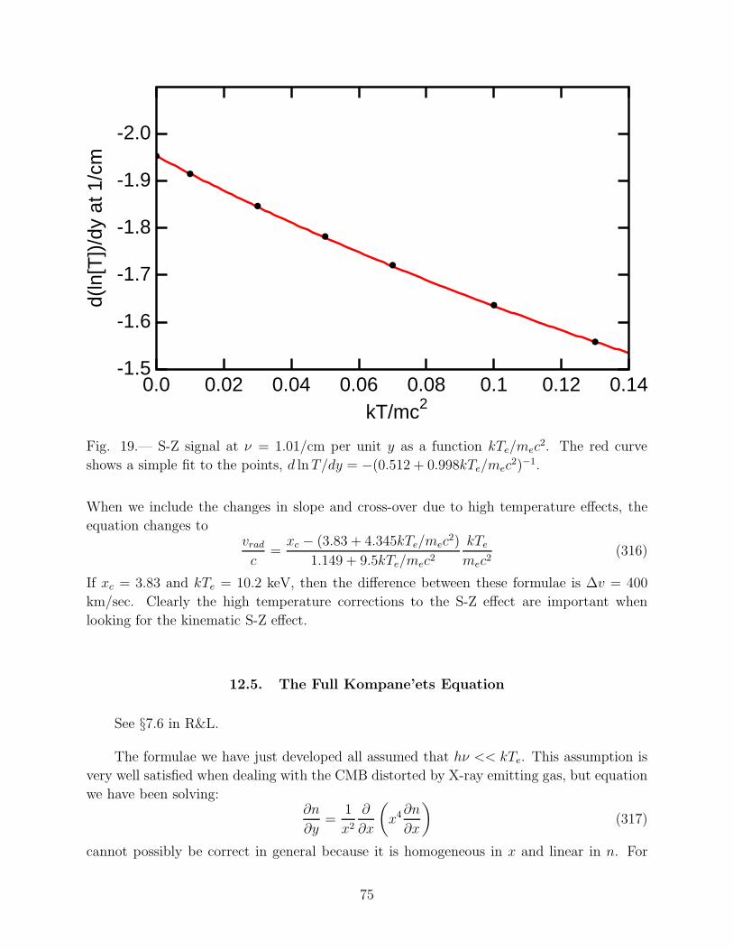
-2.0

-1.9

-1.8

-1.7

-1.6

-1.50.0 0.02 0.04 0.06 0.08 0.1 0.12 0.14

kT/mc2

d(ln

[T])

/dy

at 1

/cm

Fig. 19.— S-Z signal at ν = 1.01/cm per unit y as a function kTe/mec2. The red curve

shows a simple fit to the points, d lnT/dy = −(0.512 + 0.998kTe/mec2)−1.

When we include the changes in slope and cross-over due to high temperature effects, the

equation changes tovrad

c=xc − (3.83 + 4.345kTe/mec

2)

1.149 + 9.5kTe/mec2kTe

mec2(316)

If xc = 3.83 and kTe = 10.2 keV, then the difference between these formulae is ∆v = 400

km/sec. Clearly the high temperature corrections to the S-Z effect are important when

looking for the kinematic S-Z effect.

12.5. The Full Kompane’ets Equation

See §7.6 in R&L.

The formulae we have just developed all assumed that hν << kTe. This assumption is

very well satisfied when dealing with the CMB distorted by X-ray emitting gas, but equation

we have been solving:∂n

∂y=

1

x2

∂

∂x

(

x4∂n

∂x

)

(317)

cannot possibly be correct in general because it is homogeneous in x and linear in n. For

75

any solution f(x, y) to Eqn(317), the function Af(Bx, y) is also a solution. This makes our

convolution analysis possible, but does not have the property that a blackbody at Te will not

be affected by electron scattering. Since twice a blackbody is not a blackbody, the complete

equation must be non-linear. It also must have terms which make a blackbody a stationary

point, so something must be added to ∂n/∂x to cancel this term for a blackbody at the

electron temperature, n = 1/(ex − 1). This form gives

∂n

∂x=

d

dx

(

1

ex − 1

)

=−ex

(ex − 1)2= −(n+ n2) (318)

so the completed equation has to be

∂n

∂y=

1

x2

∂

∂x

(

x4

[

n+ n2 +∂n

∂x

])

(319)

which is the Kompane’ets equation.

Since the Kompane’ets equation is describing electron scattering, which preserves the

number of photons, one finds that the y derivative of the photon density

N = 8π(kTe)3/(hc)3

∫

nx2dx vanishes:

∂N

∂y∝

∫

x2∂n

∂ydx

=

∫

∂

∂x

[

x4

(

n+ n2 +∂n

∂x

)]

dx

=

[

x4

(

n+ n2 +∂n

∂x

)]∣

∣

∣

∣

∞

0

= 0 (320)

since the x4 factor vanishes at zero and n and dn/dx both vanish at infinity.

The stationary solutions of the equation ∂n/∂y = 0 are the photon distributions in

thermal equilibrium with the electrons. Since photons are conserved, the photon number

density does not have to agree with the photon number density in a blackbody at the

electron temperature. Thus a more general Bose-Einstein thermal distribution is allowed:

n = 1/(exp(x+ µ)− 1). This gives

∂n

∂x=

− exp(x+ µ)

(exp(x+ µ)− 1)2= −(n+ n2) (321)

Therefore ∂n/∂y = 0 for all µ.

Note that without the n2 term we would find that n+ dn/dx = 0 implies n = exp(−x)which gives a Wien distribution instead of a Planck distribution. This is also what we

saw for thermal equilibrium when ignoring stimulated emission. Thus the derivation of the

Kompane’ets equation will involve stimulated Compton scattering.

76

12.6. Derivation of the Kompane’ets Equation

If we ignore relativistic effects, the Doppler shift in scattering through an angle θ is

easily described by considering the electron velocity component along the bisector of the

scattering angle. Call this component x, so the shift is

∆ν = νvx

c2 cos(θ/2) (322)

The mean squared value of this is

var

(

∆ν

ν

)

= 4〈cos2(θ/2)〉〈v2x〉c2

= 4× 1

2× kTe

mec2= 2kTe/mec

2 (323)

This agrees with var(s) = 2y.

The mean shift corresponds to an energy transfer from the electron to the photons. This

is due to photon drag. In the electrons rest frame the intensity is anisotropic with

I(θ) = I

(

1 +4v

ccos θ

)

(324)

The scattered photons have zero net momentum so the total momentum transfer is

〈px〉 =1

4π

∫(

hν

c

)(

1 +4v

ccos θ

)

cos θdΩ =4

3

vx

c

(

hν

c

)

(325)

per scattering. The work done is

W = pxvx + pyvy + pzvz =4

3

(

hν

c

)

~v2

c= 4hν

kTe

mec2(326)

In addition to the photon drag, there is also energy transfer from the photons to the

electrons due to the Compton shift. Scattering through angle θ gives a momentum transfer

of

∆p =hν

c2 cos(θ/2) (327)

This gives a net energy transfer of

⟨

∆p2

2m

⟩

=(hν)2

mec2(328)

Thus the total energy change per scattering is

〈h∆ν〉 = hν4kT − hνmec2

(329)

77

The overall rate equation is

∂n(ν)

∂t=

(

scatterings

second

)

×∫

[P (ν1 → ν)n(ν1)(1 + n(ν))− P (ν → ν1)n(ν)(1 + n(ν1))] dν1

(330)

Now consider the electron distribution in phase space, fe(p). Consider p1 + ν1 ↔ p + ν.

Given ~p, ν, ν1 and the scattering angle Ω we know ~p1. Then

∂n(ν)

∂t= nec

∫

d3pdσ

dΩ[fe(p1)n(ν1)(1 + n(ν))− fe(p)n(ν)(1 + n(ν1))] dν1 (331)

Now we expand in powers of ν1 − ν = ∆. We now that fe(p1) = fe(p) exp(h∆/kTe) since if

ν1 has higher energy then p1 has lower energy.

Note that this assumes the electrons are not degenerate. Do not use the Kompane’ets

equation in a white dwarf.

Use x = E/kTe as the energy variable, and write hν/kTe = x

Now expand n(ν1) in powers of ∆ giving

∂n(ν)

∂t= nec

∫

d3pdσ

dΩfe(p)

[

(1 + ∆ + 12∆2)(n+ n′∆ + 1

2n′′∆2)(1 + n)

− n(1 + n+ n′∆ + 12n′′∆2)

]

d∆ (332)

The 0th order in ∆ cancels.

The 1st order in ∆ gives

n(1 + n) + n′(1 + n)− nn′.

The 2nd order in ∆ gives

12n(1 + n) + n′(1 + n) + 1

2n′′(1 + n)− 1

2n′′n.

Thus

∂n

∂t= necσT

[

(n′ + n+ n2)〈∆〉+ (12n′′ + n′(1 + n) + 1

2n(1 + n))〈∆2〉

]

(333)

But 〈∆〉 = x(4− x)(kTe/mec2) and 〈∆2〉 = 2x2(kTe/mec

2). Therefore

∂n

∂t= necσT

kTe

mec2[

x2(n′′ + 2n′ + 2nn′ + n+ n2) + x(4− x)(n′ + n + n2)]

= necσTkTe

mec2[

x2(n′′ + 2n′ + 2nn′ + n+ n2 − n′ − n− n2) + 4x(n′ + n+ n2)]

= necσTkTe

mec2[

4x(n′ + n + n2) + x2(n′′ + n′ + 2nn′)]

(334)

78

Now dy = necσT (kTe/mec2)dt and

∂

∂x

(

x4[n′ + n + n2])

= 4x3[n′ + n+ n2] + x4[n′′ + n′ + 2nn′] (335)

so the equation becomes∂n

∂y=

1

x2

∂

∂x

(

x4

[

∂n

∂x+ n + n2

])

(336)

which is the Kompane’ets equation.

The Kompane’ets equation can easily handle situations where hν ≈ kTe and it includes

the Compton shift, but its derivation used the small shift approximations requiring that

kTe <<< mec2. I do not know of any easy way to handle situations where both hν ≈ kTe

and kTe ≈ mec2. Monte Carlo simulations are simple to program except for the stimulated

scattering effect though.

13. Synchrotron Radiation

13.1. Power

Consider an electron moving in a magnetic field. The plasma in space is a good electrical

conductor so we expect zero electric field in the lab frame. Let the B field be aligned along

the z-axis. The 4 momentum of the electron will be

pµ = mc(γ; γβ sin φ cos θ, γβ sin φ sin θ, γβ cosφ) (337)

where φ is the pitch angle which remains constant, while θ is the angle around the electron’s

circular orbit and varies like dθ/dt = Ω with

Ω =eB

γmc(338)

For non-relativistic electrons the frequency is the electron cyclotron frequency: ωc = eB/mc,

or νc = (2.8 MHz/gauss)B.

If we do a Lorentz boost along the z-axis into the guiding center frame, the electron is

moving perpendicular to the magnetic field:

pµ′ = mc(γ′; γ′β ′ cos θ, γ′β ′ sin θ, 0)

B′ = B (339)

Note that while θ is unchanged in this transformation, t does change, so the new dθ/dt′ =

Ω′ = eB/γ′mc.

79

Finally do a boost along the x-axis into a frame moving at the same speed as the electron

when θ = 0. This is an inertial frame, known as the momentarily comoving inertial frame or

MCIF, while the electron’s rest frame is an accelerating frame. Usually when we talk about

the electron’s “rest frame” we mean the MCIF. In this frame we have

pµ′′ = mc(1; 0)

B′′ = γ′B

E ′′ = γ′β ′B = γβ sin φB (340)

In this frame only the electric field causes accelerations, so

a′′ =γβ sinφ eB

m(341)

and the Larmor formula gives the radiated power as

P ′′ =2

3

e2(a′′)2

c3=

2

3

e4

m2c3γ2β2 sin2 φB2 (342)

But this power is radiated in a dipole pattern in the MCIF, so the radiated power has no net

3 momentum. Thus the radiated energy-momentum is parallel to the electron’s 4 velocity,

and therefore the power dErad/dt, which is the ratio of the time components of two parallel 4

vectors, will be the same in all frames. Thus the lab power equals the MCIF power: P = P ′′.

If the pitch angles are isotropically distributed, then the average value of sin2 φ is

〈sin2 φ〉 = 2/3, giving an average synchrotron power per electron of

P =4

9

e4

m2c3γ2β2B2 =

4

3γ2σT cuB (343)

with the magnetic field energy density being uB = B2/8π and the Thomson scattering

cross-section being σT = 8πe4/3m2c4.

13.2. Spectrum

The electron’s motion is periodic with frequency Ω, but in the lab frame the received

radiated pulse is far from sinusoidal. The dipole pattern radiated by the electron has nulls

along the direction of acceleration, which are along the y′′-axis in our example. When

transformed into the guiding center frame, momentum of a photon along the y′′ axis becomes:

pµ′′ = (hν ′′/c)(1; 0, 1, 0)

→pµ′ = (hν ′′/c)(γ′; γ′β ′, 1, 0) (344)

80

E(t)

Fig. 20.— The pulse shape by an observer on the plane of the electron’s synchrotron orbit.

Ticks every mc/(2γ2eB) on the t-axis.

Thus the peak to null angle is sin−1(1/γ′). For γ >> 1 we can use small angle approximations.

Therefore the electron only turns through an angle ∆θ ≈ 1/γ′ during the pulse. Turning

through this angle takes ∆t′ = ∆θ/Ω′ = mc/eB. But the pulse as received by an observer

in front of the electron is seen in a time given by

∆trec = (1− β ′)∆t′ ≈ mc

2(γ′)2eB(345)

Thus a typical frequency for synchrotron radiation will be

ω′ =1

∆trec=

2(γ′)2eB

mc(346)

In the lab frame instead of the guiding center frame, γ′ = γ sin φ but there is a Doppler shift

factor 1/ sinφ, so this becomes

ωcrit ∝ γ2 eB

mcsin φ (347)

We can calculate the exact shape of the pulse seen by an observer situated on the plane

of the electron’s orbit in the guiding center frame. For simplicity I will drop the primes

81

on γ and β in this frame. The acceleration in the MCIF is a′ = γβeB so the radiated

electric field in the MCIF is E ′rad ∝ γβeB cos θ′. The 4 momentum of a photon in the MCIF,

(hν ′/c)(1; cos θ′, sin θ′, 0) becomes (hν ′/c)(γ(1+β cos θ′); γ(cos θ′+β), sin θ′, 0) in the guiding

center frame. Thus the Doppler shift factor is

ν

ν ′= γ(1 + β cos θ′) (348)

and the angle in the guiding center frame is given by

sin θ =py

|p| =sin θ′

γ(1 + β cos θ′)(349)

Now the radiated field transforms like the Doppler shift factor squared to keep the number

of photons per mode invariant. Hence

Erad ∝ eBγ3β(1 + β cos θ′)2 cos θ′ (350)

Now we need to calculate the received time, trec = t − x/c. We know that x = R sin Ωt =

R sin θ. Let’s let

y =sin θ′

1 + β cos θ′(351)

Then

trec =θ

Ω− R

csin θ

=1

Ωsin−1

(

y

γ

)

− R

c

y

γ

=γmc

eB

(

y

γ+

1

6

(

y

γ

)3

+ . . .

)

− γβmc

eB

y

γ

=mc

eB

[

(1− β)y +y3

6γ2+ . . .

]

=mc

2γ2eB

[

y +y3

3

]

(352)

We have already assumed β ≈ 1 in 1− β = 1/(2γ2), so continuing to use β ≈ 1 gives us

y2 =sin2 θ′

(1 + cos θ′)2=

1− cos2 θ′

(1 + cos θ′)2=

1− cos θ′

1 + cos θ′(353)

Hence

cos θ′ =1− y2

1 + y2(354)

and

1 + cos θ′ =2

1 + y2(355)

82

Thus we get

Erad(trec) ∝ eBγ3 1− y2

(1 + y2)3(356)

at

trec =mc

2γ2eB

[

y +y3

3

]

(357)

We can of course find the spectrum by Fourier transforming this pulse, giving

E(ω) ∝∫

1− y2

(1 + y2)3eiωtdt (358)

Inverting the equation for y as a function of t introduces branch cuts but we can still find

the dominant high frequency behaviour by locating the pole closest to the real t-axis in the

upper half of the complex t plane. This is at y = +i which gives

tpole =mc

2γ2eB

(

i− i

3

)

=imc

3γ2eB(359)

The high frequency cutoff in E(ω) thus goes like

E(ω) ∝ exp

[

− mc

3γ2eBω

]

|E(ω)|2 ∝ exp

[

− 2mc

3γ2eBω

]

= exp

[

− ω

ωcrit

]

(360)

with a critical frequency that is just 1.5γ2 times the cyclotron frequency:

ωcrit =3

2

eB

mcγ2

νcrit =ωcrit

2π= (4.2 MHz/gauss)B (361)

The integral for E(ω) can be done exactly by changing the variable of integration to y

with dt = (1 + y2)dy, giving

E(ω) ∝∫

1− y2

(1 + y2)2exp

[

iωmc

2γ2eB

(

y +y3

3

)]

dy (362)

Integrate by parts (∫

pdq = pq −∫

qdp) using q = y/(1 + y2) so dq = (1 − y2)dy/(1 + y2)2,

and p = exp[. . .] so dp = (iωmc/(2γ2eB))(1 + y2) exp[. . .], giving

E(ω) ∝ ω

∫

y exp

[

iωmc

2γ2eB

(

y +y3

3

)]

dy ∝ ωK2/3(ω/(3γ2eB/mc)) (363)

83

which has the exponential high frequency cutoff we found earlier and behaves like ω1/3 for low

frequency. This would give a power going like ω2/3 but the total power radiated, integrated

over all angles instead of just for an observer in the plane of the orbit, is given by

P (ω) ∝ F

(

ω

ωcrit

)

F (x) = x

∫ ∞

x

K5/3(y)dy (364)

which goes likes ω1/3 for low frequencies.

As discussed earlier, the critical frequency varies with pitch angle as sinφ. For a tangled

magnetic field and an isotropic pitch angle distribution, we observe a power ∝ sin2 φ with

critical frequency 1.5 sinφ γ2eB/mc. The power weighted mean of sinφ is∫

sin3 φ dΩ∫

sin2 φ dΩ=

2π∫

sin4 φ dφ

8π/3=

3

4

∫ π

0

[(1− cos(2φ))/2]2dφ =9π

32(365)

Thus the power weighted mean critical frequency is

3

2× 9π

32× eB

mcγ2 = 1.325

eB

mcγ2 (366)

I recommend remembering this factor 1.325 as 4/3.

13.3. Power Law Distributions

In most astrophysical sources the relativistic electrons producing synchrotron radiation

have γ’s that cover a wide range: usually a few decades or more. Because of this, the

synchrotron radiation spans several decades, but the exact spectral function F (x) is not so

wide. It is therefore appropriate to ignore the width of F (x) and to approximate it by a

delta function! We will assume the following very simple form for the power emitted by

mono-energetic electrons with random pitch angles in a tangled magnetic field:

P (ν) =4

3γ2cσTuBδ

(

ν − 4

3

γ2eB

2πmc

)

(367)

With this approximation it is easy to compute the synchrotron power generated by a popu-

lation N(γ) of electrons per unit γ. With 2πν = (4eB)/(3mc) we get

Lν =

∫

4

3γ2cσTuBδ(ν − νγ2)N(γ)dγ =

2γN(γ)cσTuB

3ν

∣

∣

∣

∣

γ=√

ν/ν

(368)

An easier way to remember this is

νLν =

(

γN(γ)

2

)(

4

3γ2cσTuB

)

(369)

84

which is (power/octave) = (electrons/half-octave) times (power/electron). Only a half-

octave in the electron distribution is used because the quadratic dependence of ν on γ

means that a half-octave in γ covers a full octave in ν.

For a power law N(γ) ∝ γ−β, we get a power law spectrum. From

Lν ∝ γN(γ) ∝√

ν/νN(

√

ν/ν

)

∝ ν(1−β)/2 (370)

we see that the power index in Lν ∝ ν−α is

α =β − 1

2(371)

Thus the power law index β = 2.5 seen in the cosmic rays translates into α = 0.75 which is

a typical spectral index for a non-thermal radio source.

13.4. Energy in Relativistic Particles

The relation between synchrotron emission and the number of electrons with γ’s close

to√

ν/ν allows us to compute the total energy in relativistic electrons in a radio source

from its synchrotron spectrum. We can write

Epart =

∫

N(γ)γmc2dγ (372)

and

γN(γ) =3νLν

2cσT uB

(373)

But dγ = γdν/(2ν) so

Epart =

∫

3νγmc2Lν

4cσT uB

dν

ν=

∫

3√ννmc

2Lν

4cσT uB

dν

ν(374)

which becomes

Epart =

√24πemc

σT

B−3/2

∫ √νLνd ln ν = 1.5× 1012B−3/2

∫ √νLνd ln ν (375)

in cgs units. Thus if we know the magnetic field, we can compute the energy in relativistic

electrons needed to produce the observed synchrotron radiation.

In the local ISM the cosmic ray energy density approximately equals the magnetic field

energy density. Since the cosmic rays are only held to the galaxy by the magnetic field, if

the magnetic field energy density was less than the cosmic ray energy density the cosmic

rays would rapidly escape. And apparently if the cosmic ray energy density is less than

85

the magnetic field energy density Alfven turbulence accelerates cosmic rays until the energy

densities are comparable. If we assume the energy density in relativistic electrons equals

the magnetic field energy density, we derive the equipartition magnetic field strength for a

radio source. As seen above, the particle energy is Epart = AB−3/2 where is A depends on

observed quantities and constants. The magnetic field energy is Emag = B2V/8π where V is

the volume of the source. Setting these equal gives

Beq =

(

8πA

V

)2/7

(376)

We can also find the B that minimizes the total energy needed to produce the observed

synchrotron emission,

BME =

(

6πA

V

)2/7

(377)

The difference between these is an insignificant factor of 0.752/7 = 0.92.

A more significant problem is the protons. In the local cosmic rays, we see about

dN/dE = 1× E−2.5 protons/cm2/sec/sr/GeV and 0.01× E−2.5 electrons/cm2/sec/sr/GeV.

So it might be reasonable to assume that Epart should be multiplied by 100 to allow for

relativistic protons which we cannot see because they don’t radiate synchrotron emission.

This would increase Beq by a factor of 1002/7 = 3.7. But if we compute N(γ) at γ = 2000

for the protons we find 6.1 × 10−9 while for electrons we find N(γ = 2000) = 4.8 × 10−6.

Thus while electrons of a given energy are 100 times less common that protons of the same

energy, electrons of a given γ are 800 times more numerous than protons of the same γ. As

a result, we don’t know whether to apply the proton correction to Beq.

13.5. Synchrotron Self-Absorption

A population of relativistic electrons produces a synchrotron emissivity of

4πjν =2γn(γ)cσTuB

3ν

∣

∣

∣

∣

γ=√

ν/ν

(378)

where n(γ) is the number density of electrons per unit γ. If there were no corresponding

absorption process, then a line of sight with a very long path length through a synchrotron

source would have an intensity that grew without limit as the path length increased. But

there is a synchrotron absorption process, and we can calculate its magnitude using Kirchoff’s

law: Bν(Tex) = jν/αν . But what is the excitation temperature Tex for the transitions involved

in synchrotron emission? What are the quantum levels?

The orbits of electrons around the magnetic field lines are actually quantized with

angular momenta in units of ~. The angular momentum is pR and R = pc/eB so the quantum

86

number is n = p2c/~eB = γ2β2m2c3/~eB. We can write this as n = γ2β2Bcrit/B where

Bcrit = 5 × 1013 gauss is the magnetic field that makes the cyclotron frequency equivalent

to the electron rest mass. For a typical γ = 104 and B = 10−4 gauss, n = 5 × 1021, so a

purely classical description of synchrotron emission is appropriate. The typical transition in

synchrotron emission is not ∆n = 1, but rather ∆n ≈ γ3, so both n and ∆n can be taken

to be continuous variables. This gives

kTex =∆E

ln(n1/g1)− ln(n2/g2)⇒ kTex = −

(

∂ ln(n/g)

∂E

)−1

(379)

Now we need to know the statistical weight g for states in a unit range of γ. This is given

by phase space volume in units of h3, g = gsd3pd3x/h3, where gs = 2 is the statistical weight

for spins. The volume factor dx3 cancels out, and for the ultrarelativistic limit, γ >> 1, we

have d3p ∝ γ2dγ. Therefore, when n(γ) ∝ γ−β, the excitation temperature is

kTex = −(

∂ ln(γ−(β+2))

mc2∂γ

)−1

=γmc2

β + 2(380)

Since γ =√

ν/ν, and since kTex is always much greater than the energy of the photons

seen from synchrotron sources, when a source is optically thick to synchrotron emission its

surface brightness varies like Iν ∝ ν2.5.

Thus observing the surface brightness of an optically thick sychrotron source gives the

γ factor, and γ plus ν together give the magnetic field. Since the surface brightness is very

high, with brightness temperatures >> mc2/k = 6 × 109 K, optically thick synchrotron

sources always have very small angular sizes and can only be resolved by Very Long Baseline

Interferometry (VLBI). A source with brightness temperature of 1012 K at 5 GHz with an

angular size of 0.001′′ has a flux of Fν = 2kT (ν/c)2Ω ≈ 20 Jy.

14. Inverse Compton Scattering

Consider an electron moving relativistically through an isotropic distribution of photons

with energy hν. A photon approaching with angles π − θ to the electron’s velocity (θ = 0

for a head-on collision) has 4-momentum

pµ =hν

c(1;− cos θ,− sin θ, 0) (381)

if we make the x axis the electron’s velocity vector and put the photon direction in the xy

plane. Let µ = cos θ. Then the photon momentum in the electron’s rest frame is

pµ′ =hν

c(γ(1 + βµ);−γ(β + µ),− sin θ, 0) (382)

87

Now let the photon scatter off the electron, leaving with angle θ′ to the x axis. For now

we ignore the true Compton shift, so the energy of the outgoing photon is hν ′′ = hν ′ =

(γ(1 + βµ))hν. Note that θ′ = 0 corresponds to a photon traveling in the same direction as

the electron, while θ = 0 corresponds to a photon traveling in the opposite direction as the

electron. The 4 momentum after scattering is

pµ′′ =hν ′′

c(1; cos θ′, sin θ′, 0) (383)

Now let µ′ = cos θ′. Then the 4 momentum after scattering back in the lab frame is

pµ′′′ =hν ′′

c(γ(1 + βµ′); γ(β + µ′), sin θ′, 0) (384)

We finally get the ratio of the lab frame energy after scattering to the lab frame energy

before scattering:ν ′′′

ν= γ2(1 + βµ)(1 + βµ′) (385)

We want to find the average value of this ratio, which will tell us the total energy transfer

from the electron to the photons, and also the typical frequency of the output photons. In

order to find the average, we need to know the probability distributions for the scattering

angles µ and µ′.

A first guess would be that p(µ) should be a uniform distribution since this corresponds

to an isotropic initial photon field because dΩ = 2πdµ. But head-on collisions (µ = 1)

will happen more frequently than stern chase collisions (µ = −1). In fact, the rate of

photon collisions has exactly the same Doppler shift factor as the photon frequency, so

p(µ) ∝ γ(1 + βµ). Normalizing this in the range −1 < µ < 1 gives the probability density

function (pdf):

p(µ) =1 + βµ

2(386)

Note the function you integrate to find probabilities in a given distribution is called the

probability density function and should not be confused with the distribution. Rybicki &

Lightman approximate the distribution of µ′ with a uniform distribution, corresponding to

isotropic scattering. This gives a pdf

p′R&L(µ′) =1

2(387)

With this approximation we can easily find the average ratio:⟨

ν ′′′

ν

⟩

=

∫ ∫

γ2(1 + βµ)(1 + βµ′)p(µ)p′(µ′)dµdµ′

= γ2

∫

(1 + βµ)2

2dµ

∫

1

2(1 + βµ′)dµ′

= γ2

(

1 +β2

3

)

(388)

88

The ultrarelativistic limit is (4/3)γ2.

However, electrons do not scatter isotropically. If the actual scattering angle is ψ, the

scattering rate is proportional to (1 + cos2 ψ). We can write cosψ as

cosψ = −(

µµ′ +√

1− µ2√

1− µ′2 cosφ)

(389)

where φ is the dihedral angle between the plane defined by the x axis and the incoming

photon and the plane defined by the x axis and the outgoing photon. The rate of scattering

into µ′ will be proportional to the average of (1 + cos2 ψ) over all φ’s. Thus the true pdf

p′(µ′) for Rayleigh scattering electrons is given by

p′(µ′;µ) =3

8

∫ 2π

0

(1 + cos2 ψ)dφ

2π

=3

8

∫ 2π

0

[

1 + µ2µ′2 + 2µµ′√

1− µ2√

1− µ′2 cosφ+ (1− µ2)(1− µ′2) cos2 φ] dφ

2π

=3

8

[

1 + µ2µ′2 +1

2(1− µ2)(1− µ′2)

]

=3

8

[

3

2(1 + µ2µ′2)− 1

2(µ2 + µ′2)

]

(390)

The (3/8) factor normalizes the pdf:

∫

p′(µ′;µ)dµ′ =3

8

[

3 + µ2 − µ2 − 1

3

]

= 1 (391)

for any value of µ. Note that the distribution of µ′ does depend on µ, but is this dependence

is not the probability density function for µ. By writing µ following a semicolon, we mean

that µ is a parameter that modifies the µ′ distribution. The joint pdf for µ and µ′ is given

by

p(µ, µ′) = p(µ)p′(µ′;µ) (392)

But the pre-scattering angle we need is not really µ, which is measured in the lab frame,

but rather the pre-scattering angle in the electron’s rest frame, whose cosine is given by

(β + µ)/(1 + βµ). We can now find the average ratio:

⟨

ν ′′′

ν

⟩

=

∫ ∫

γ2(1 + βµ)(1 + βµ′)p(µ)p′(µ′; (β + µ)/(1 + βµ))dµdµ′

= γ2

∫

(1 + βµ)2

2dµ

×∫

3

8

[

3

2

(

1 +

[

β + µ

1 + βµ

]2

µ′2

)

− 1

2

(

[

β + µ

1 + βµ

]2

+ µ′2

)]

(1 + βµ′)dµ′

= γ2

(

1 +β2

3

)

(393)

89

To get the last line of this result, note that p′(µ′) is always an even function of µ′, so∫

βµ′p′(µ′)dµ′ = 0 and the integral∫

(1 + βµ′)p′(µ′)dµ′ = 1 Thus the average is exactly the

same as the result calculated in the isotropic scattering approximation used by Rybicki &

Lightman.

14.1. Power Law Sources

Using the mean energy increase factor, we find that an ultrarelativistic electron loses

energy by the inverse Compton process at a rate

PIC =4

3γ2c σT uph (394)

where uph is the energy density of the photons the electron is colliding with. The typical

output frequency is

νIC =4

3γ2νin (395)

where νin is the typical frequency of the photons the electron is colliding with. Thus a dis-

tribution of relativistic electrons N(γ) produces an inverse Compton source with luminosity

νLν =

(

γN(γ)

2

4

3γ2cσTuph

)∣

∣

∣

∣

γ=√

ν/ν1

(396)

with ν1 = (4/3)νin. The relationship between N(γ) and the spectrum is exactly same for

inverse Compton sources and synchrotron sources. The the shapes of the spectra on a log-log

plot will be identical, but the scaling in luminosity and in frequency will be different.

But what are the typical sources of input photons? Three are important: the cosmic

background radiation, starlight, and a source’s own synchrotron radiation for compact radio

sources. The CMBR is universal, so we will concentrate on it. The energy density is

uCMBR = aT 4 =

4σ

cT 4 = 4× 10−13 erg/cm3 (397)

This is equivalent to the magnetic field energy density from a field of B = 3.3 µG. The

typical frequency is ≈ 3kT/h = 1.7 × 1011 Hz. Thus if both the IC off the CMBR and

synchrotron emission from a source are detected, the magnetic field can be determined from

both the ratio of νLν ’s and from the ratio of frequencies. The relations to use are:

(νLν)IC

(νLν)S

=

(

3.3 µG

B

)2

(398)

andνIC

νS=

6× 104 G

B(399)

90

Thus for a typical radio source the IC luminosity is much less than the synchrotron luminosity

but it peaks at a much higher frequency. Typically the IC flux is in X-rays or γ-rays. An

upper limit on the X-ray or γ-ray flux from a radio source gives a lower limit on the magnetic

field.

When a radio source is very compact the synchrotron flux it emits can have an energy

density larger than the CMBR. This energy density of synchrotron photons can then be

scattered by relativistic electrons, producing X-rays by what is called the synchrotron-self-

Compton process. The fraction of synchrotron photons scattered is about τ , where τ is

the optical depth to electron scattering from the relativistic electrons. The energy of the

scattered photons is boosted by a factor of (4/3)γ2. If the product (4/3)γ2τ is greater than

one, then the IC photons will have a larger energy density than the synchrotron photons,

and one will get second-order IC emission. This process continues until the energy in the

electron’s rest frame is comparable to mc2. The IC photons produced in this step have

energy γmc2 – which is all of the electron’s energy. This cascading of the IC process puts out

energy in the γ-ray region of the spectrum, instead of the radio region. Since some quasars

are compact radio sources, the IC cascade has been called “the Compton catastrophe” in

quasar models. But since quasars are also γ-ray sources, it isn’t all bad.

14.2. Details

We already have the most important results: the mean energy increase factor. But the

distribution of output energies is also good to know. The maximum possible output:input

ratio is γ2(1+β)2, but since γ2 = (1−β2)−1 = (1+β)−1(1−β)−1, the maximum energy can be

written as (1 + β)/(1− β), which is the square of the relativistic Doppler shift formula. The

minimum possible output to input ratio is γ2(1−β)2 which can be written as (1−β)/(1+β).

Note that this is just one over the maximum ratio.

Let R = ν ′′′/ν be the output:input ratio. Then we can find the pdf for R using

pR(R) =

∫ ∫

δ(R− γ2(1 + βµ)(1 + βµ′))p(µ)p′(µ′;µ)dµdµ′ (400)

In the isotropic approximation this is easy to evaluate: do the integral over µ′ first, so the

delta function integrates to [γ2β(1 + βµ)]−1. This cancels the µ dependence of p(µ), so the

result for pR(R) is proportional to the amount of the µ range that is compatible with a given

R. This is all of it for R = 1, and from µ = β−1[(1 − β)R − 1] to 1 for R > 1. Thus

pR(R) declines as a linear function of R from a maximum at R = 1 to zero at R = Rmax =

(1 + β)/(1 − β). For R < 1 the range in µ is from -1 to µ = β−1[(1 + β)R − 1], so again

pR(R) declines linearly from the maximum at R = 1 to zero at R = Rmin = (1− β)/(1 + β).

Finally we should calculate the mean squared output:input ratio. In the isotropic ap-

91

proximation used by R&L, this quantity is⟨

(

ν ′′′

ν

)2⟩

=

∫ ∫

γ4(1 + βµ)2(1 + βµ′)2p(µ)p′(µ′;µ)dµdµ′

= γ4

∫

(1 + βµ)3

2

∫

(1 + βµ′)2

2dµ′dµ

= γ4

∫

(1 + βµ)3

2

[

1 +β2

3

]

dµ

= γ4[

1 + β2]

[

1 +β2

3

]

= γ4

[

1 +4

3β2 +

1

3β4

]

(401)

This differs from the exact result only in the β4 term.

15. Plasma Effects

Chapter 8 of R&L

15.1. Dispersion

Assume that the electrons in the plasma are moving with β << 1. An electromagnetic

wave has | ~E| ≈ | ~B| (exactly equal in a vacuum of course) which means that the force due to

the wave’s magnetic field can be neglected. However, there can be a static magnetic field in

the plasma, ~B. For a wave with time dependence ∝ e−iωt, we get

−imω~v = −e( ~E + c−1~v × ~B) (402)

We need to calculate the dielectric constant of the medium, ǫ, in order to calculate the phase

velocity of the wave, vp = c/√ǫµ, since µ = 1.

Now the dielectric constant is

ǫ = 1 + 4πχ (403)

where the permittivity χ is the ratio of the dipole density to the applied electric field. The

dipole density is −enex = −ene~v/(−iω). Since both the electric field and the dipole density

are vectors, χ is a tensor. In order to simplify the analysis, take the magnetic field to be

along the z-axis. Then an electric field along the z-axis generates velocities along the z-axis,

which give zero cross product with B, so the z behavior separates out, giving:

vz =−ieEz

mω(404)

92

Since x = v/(−iω) and the dipole density is −neex, one has

χzz =−e2ne

mω2(405)

ǫ = 1− 4πe2ne

mω2= 1−

(ωp

ω

)2

(406)

where the plasma frequency is ωp =√

4πe2ne/m.

The index of refraction is n =√ǫ. Because of variations in the electron density, rays are

bent as they travel through the interstellar medium. This leads to interstellar scintillation

for point-like radio sources. The equation for ray paths in refraction is

d(nk)

ds= ~∇n (407)

following Eqn (8.18) in R&L. Since n is less than one, convex concentrations of electrons

yield diverging lenses.

The intensity I is not then conserved along a ray, but rather I/n2.

Phase vs. group velocity

Note that for ω < ωp, the dielectric constant is negative, which gives an imaginary phase

velocity. Thus the wave vector k = ω/vp is also imaginary, so the spatial propagation ∝ eikx

gives a decaying exponential instead of a propagating wave. Thus waves below the plasma

frequency are absorbed. The relationship between k and ω, known as the dispersion relation,

is

c2k2 = (ω2 − ω2p) (408)

For ω > ωp the dielectric constant is positive but less than unity. This implies a phase

speed that is faster than the speed of light. How can this be if no thing can travel faster

than the speed of light? The wave crests in a pulse don’t correspond to signals, but the peak

of the amplitude of a pulse composed of several frequencies does correspond to a photon or

signal. Consider a propagating pulse with complex amplitude A(ω). Then the electric field

will be

E(x, t) =

∫

A(ω) exp(ikx− iωt)dω (409)

The amplitude of this pulse will be maximized at the x where the phase of the integrand is

constant near the peak of |A|. Let A = |A|eiφ and assume that dφ/dω = 0 at the peak of

|A|. This corresponds to the pulse peaking at x = 0 when t = 0. At a later time t > 0, the

location of the peak of the pulse is found by setting

d[φ+ kx− ωt]/dω = 0 = dφ/dω + xdk/dω − t = 0 (410)

93

Thus the peak is at x = (dω/dk)t and the group velocity which describes the motion of the

peak is

vg =dω

dk(411)

The value of the group velocity can be found using

vpvg =ωdω

kdk=d(ω2)

d(k2)= c2 (412)

since the dispersion relation gives a linear relation between k2 and ω2 with a slope of c2.

Thus the group velocity of the wave with an electric field parallel to the static magnetic

field is

vg = c

√

1−(ωp

ω

)2

(413)

If a broadband pulse is emitted simultaneously at all frequencies, then it will be received

first at high frequencies, then later and later at lower and lower frequencies. This turns the

pulse into a falling chirp instead of a click. The time it takes for a given frequency to arrive

is given by

tν =

∫

ds

vg≈∫

(1 +ν2

p

2ν2)ds

c=

∫

ds

c+

e2

2πmcν2

∫

neds (414)

With the dispersion measure DM being∫

neds in units of cm−3pc, the delay for frequency

ν is

∆tν = 0.415 DM

(

100 MHz

ν

)2

sec (415)

For pulsars the difference in delay times between two different frequencies is easily

measured, giving a determination of DM . For a few pulsars distances can be estimated,

and the typical ratio of DM to distance is the mean electron density in the ISM, 〈ne〉 =

0.03 cm−3. For other pulsars distances can be estimated from the dispersion measure: dis-

tance ≈ DM/〈ne〉.

15.2. Rotation Measure

The components of the velocity perpendicular to the magnetic field get coupled by the

cross product, so the equations for vx and vy are:

−imωvx = −e(Ex + c−1vyBz)

−imωvy = −e(Ey − c−1vxBz) (416)

If we consider v+ = vx + ivy we get an equation

vx + ivy = −i(e/mω)(Ex + iEy + c−1Bz(vy − ivx)) (417)

94

or

v+ = −i e

mωE+ −

eBz

mcωv+ (418)

with E+ being Ex + iEy, a circularly polarized wave. Thus

v+ = −i e

m(ω + ωB)E+ (419)

where ωB is the cyclotron frequency eB/mc. For the opposite sense for circular polarization,

it is clear that

v− = −i e

m(ω − ωB)E− (420)

The displacement x is still x = v/(−iω), so the dielectric constants for the two circular

polarizations are

ǫR,L = 1− ω2p

ω(ω ± ωB)(421)

Over a path, the accumulated phase is

φR,L ≈∫(

ω − ω2p

2(ω ± ωB)

)

ds

c(422)

Thus the phase difference between the right and left circularly polarized waves is

φR − φL = ∆φ ≈∫

ω2pωB

ω2

ds

c(423)

The rotation of a plane-polarized wave is ∆θ = ∆φ/2, so

∆θ =

∫

ω2pωB

2ω2

ds

c(424)

which for a constant B is just ∆θ = ωB∆tν . The average magnetic field along the line of

sight, weighted by electron density, is found using

〈B||〉 =

∫

ne~B · ~ds

∫

neds=mc∆θ

e∆tν(425)

In general we don’t know the original angle of polarization (or the time of emission), but

we can measure the change in polarization angle between two frequencies and compare it

to the change in arrival time between the same two frequencies for pulsars, giving a well

determined 〈B||〉. In the ISM this field is 2.5 µG. In typical synchrotron sources the emission

is polarized so∫

ne~B · ~ds can be found, but without pulses one needs to assume an ne to get

a magnetic field estimate.

95

10-23

10-22

10-21

10-20

10-19

10-18

10-17

10-16

10-15

10-14

10-13

10-12

10-11

10-10

0.001 0.01 0.1 1 10Period [sec]

|dP

/dt|

10 7 G

10 10 G

10 13 G

104 yr

108 yr

1012 yr

Death

Line

Fig. 21.— The distribution of 1743 known pulsars in the P -P plane. The orange dots have

negative P , probably due to gravitational acceleration in the galaxy or a globular cluster.

The magenta dots are recently discovered occasional pulsars that only emit a pulse several

times per day, even though their rotation periods are a few seconds (astro-ph/0511587). The

green dots are γ-ray only pulsars from Pletsch et al.(arXiv:1111.0523). The red dots are the

components of the double pulsar, J0737-3039. The blue dashed line shows the empirical

“death line” for radio pulsars, with P ∝ P 3. The few points in the far upper right are

the so-called “magnetars” or anomalous X-ray pulsars. The main clump of points are the

“young” pulsars. The points in the lower left are the “recycled” pulsars that were spun up

by accretion in a binary system.

96

16. Pulsar Emission

One of the most interesting astrophysical E&M emissions are pulses from pulsars. This

is also one of the least well understood processes, but a few basic ideas can be easily stated.

Pulsars are rapidly rotating neutron stars with very large magnetic fields. The energy that

drives the emission is coming from the rotational kinetic energy for radio pulsars. Therefore

the pulse rate is slowing down. One can define a spindown or characteristic age using the

pulse period P and the spindown rate P . A characteristic time is P/P . The moment of

inertia of a neutron star is about 1045 gmcm2, and the rotational kinetic energy is E =

0.5 Iω2 ≈ 1048(140 ms/P )2 ergs. For a rapidly spinning pulsar like the Crab pulsar this

kinetic energy is larger that the total light output of a supernova, 1049 ergs. The spindown

luminosity is

L = −Iωω = 4π2IP /P 3. (426)

This luminosity is usually assumed to be magnetic dipole radiation. An electric dipole with

a charge −q at the origin and a charge q at z << R has a dipole moment of µe = qz and a

field at the pole z = R of Ep = 2qz/R3. Therefore µe = 0.5EpR3. Thus the magnetic dipole

moment of a neutron star with polar surface field of Bp and radius R is µm = 0.5BpR3. The

power radiated by a spinning electric dipole is P = (2µ2eω

4/3c3) and the power radiated by

a spinning magnetic dipole is P = (2µ2mω

4/3c3) due to the nice symmetry between electric

and magnetic quantities in cgs units. Setting this equal to the spindown luminosity gives

B2p R

6 ω4

6c3= −Iωω (427)

so an estimate for the surface magnetic field is given by

Bp =

(

6c3I

4π2R6

)0.5√

PP = 2× 1012 gauss

(

I

1045

)0.5(R

10 km

)−3(

P

1 sec

P

10−15

)0.5

(428)

The equatorial magnetic field is half this, so Beq = 3.2×1019√

PP G. Note that this assumes

an oblique rotator where there is an angle θ = π/2 between the dipole axis and the spin axis.

For general θ the luminosity goes like sin2 θ. Because ω ∝ −ω3 if B is constant, we find that

∆ω−2 ∝ ∆t or P ∝ t1/2. Therefore the characteristic age of a pulsar is taken to be

τ =P

2P. (429)

For the Crab nebula pulsar the characteristic age is 1240 years while the actual age is 960

years. The Crab nebula pulsar emits about 1030.5 erg/sec in the radio and 1035 erg/sec

at IR through γ-ray wavelengths, but the spin down luminosity is 1038.4 erg/sec which is

much larger. Clearly 99.9% of the spindown luminosity must go into accelerating relativistic

particles which power the Crab nebula itself.

The “death line” is the observed boundary of the pulsar distribution, as shown in Figure

21. It has been described as B/P 2 = 0.17 × 1012 Gauss/sec2 which would give P ∝ P 3

97

(Faucher-Giguere & Kaspi, astro-ph/0512585, heareafter F-G&K). This corresponds to a

spin-down luminosity of −E = 1030.1 erg/sec. F-G&K find that the radio luminosity of a

pulsar is on average proportional to the square root of the spin-down luminosity.

F-G&K find that pulsars are born with a broad range of periods, Pbirth = 300±150 mil-

liseconds.

Pulsar positions can be measured very accurately by timing. The motion of the Earth

produces a ±500 cosβ second variation of pulse arrival times with a one year period whose

phase gives the ecliptic longitude. β is the ecliptic latitude. Since pulse arrival times can be

measured to µsec accuracy the angular position can be found to milli-arcsecond accuracy.

Proper motions and occasionally parallaxes can also be measured. The studies of proper

motions show that pulsars are typically born with a “kick” velocity broadly distributed

around a mean of 380 km/sec.

The interstellar plasma causes a dispersion of pulses into chirps with low frequencies

arriving later, and this dispersion measure can be used to estimate distances to pulsars.

Since pulsar pulses are quite narrow in rotational longitude, it is expected that the beam

is also narrow in latitude. Then only a small fraction of pulsars will be observable from the

Earth. Using a model which gives a 10% average for this beaming fraction, F-G&K get a

pulsar birth rate of 2.8/century in the Milky Way.

Pulsar radio emission mechanisms are not well understood. But it is clear that coherent

emission by a large number of charges moving together must be involved. For a flux of 1

Jy at a frequency of 100 MHz from a source of radius 10 km at a distance of 1 kpc the

brightness temperature is

Te =Iν

2k(ν/c)2=

10−23 × 90000× (3.08× 1021)2

2× π × (106)2 × 1.38× 10−16= 1028 K (430)

which is too high to come from single electron processes. In order to produce a large number

of charges it is thought that γ-ray photons produced by curvature radiation must have enough

energy to allow pair production by colliding with the virtual photons of the pulsar magnetic

field. The cyclotron frequency in a Teragauss field is 11 keV so 25 MeV γ-rays are needed.

Radiating 25 MeV photons by synchrotron radiation in a field with a cyclotron frequency

of 11 keV requires electrons with γ = 50. An electron with this energy has a synchrotron

lifetime of 10−17 sec in a magnetic field of 1012 gauss so the pitch angles will rapidly decay

to zero. Then the radiation is caused by curvature radiation, where the radius is determined

by the curvature of the field line instead of pc/eB.

The field lines in a dipole field are in fact circles, but even for more general shapes we only

need to look at the local radius of curvature. If we calculate an effective magnetic field that

would give the same radius as the curvature of the field line we get γβmc2 = eBeffR. Then

98

the critical energy for curvature radiation can be found using the formulae for synchrotron

radiation in this field. We should not average over pitch angles in this calculation. This

gives

ωc = 1.5γ2 eBeff

mc= 1.5γ3β

c

R(431)

For this to reach 25 MeV requires that γ = 106. We can calculate the power radiated just

from the motion of the electron around a circle, with an acceleration a = v2/R which is

increased by a factor of γ2 in the MCIF. The power per electron radiated by curvature

radiation is then

P =2e2a2

3c3=

2γ4β4e2c

3R2(432)

For γ = 106 this is 4600 erg/sec for R = 10 km. Thus an electric field of E = P/ec is needed

to keep the electrons going fast enough to emit 25 MeV γ-rays. Converting the power into

eV/sec and then dividing by c gives an electric field of E = 105 Volt/cm. In cgs units this

is 300 statvolts/cm which is 3 billion times smaller than the magnetic field.

16.1. γ-ray Pulsars

Many radio pulsars have been seen in pulsed γ-rays, but with the Fermi Gamma-ray

Space Telescope the γ-ray observations are sensitive enough to find pulsars that cannot be

seen in radio observations. Pletsch et al.(arXiv:1111.0523) found 9 γ-ray pulsars but only

one could be seen in radio emission.

17. Magnetic Dipole Emission

As discussed for pulsars, a time-varying magnetic dipole produces the same radiated

power as a time-varying delectric dipole because in cgs units the magnetic field has the units

as the electric filed, and a magnetic dipole has the same units as an electric dipole. But

magnetic dipole transitions are considered to be forbidden transitions. Why is this so?

Consider an electron orbiting around with an orbit radius of a = 0.53 A, with velocity

v. If there is an applied magnetic field B in the plane of the orbit, the electron feels a force

F = e(v/c)B cos θ with a lever arm a cos θ, where θ is the angle around the orbit, so the

torque obtained by averaging around the orbit is T = 0.5e(v/c)aB and the magnetic dipole

is µorb = 0.5e(v/c)a. Typically (v/c) = α = 1/137 so the magnetic dipole is more than 100

times smaller than a typical electric dipole of O(ea).

Note that ~2/(2mea

2) = 0.5e2/a giving a = ~

2/(mee2), vt = ~/(mea) = e2/~ = αc.

Thus µorb = 0.5e(e2/~c)(~2/(mee2)) = 0.5e~/mec = µB, the Bohr magneton.

99

Thus magnetic dipole transitions typically have Einstein A values that are α2 or O(104)

times smaller than electric dipole transitions.

18. Molecular Hydrogen Emission

The most common molecule in the Universe is H2, but because it is homo-nuclear it has

no permanent dipole moment. As a result, the vibrational-rotational emission from H2 is

“forbidden”, and occurs through the weak channel of electric quadrupole radiation.

For a typical quadrupole moment of Q = ea2 compared to a typical dipole moment

of µ = ea, the electric quadrupole interaction energy which goes like ~∇ ~EQ is ka times

smaller than the dipole interaction energy µ · ~E. Since the wavenumer k is about 105/cm

for electronic transitions and 103/cm for infrared transitions, the electric quadrupole lines

will be 106 to 1010 times weaker than electric dipole lines. If an electric dipole line at 82,300

cm−1 has an Einstein A = 6×108 sec−1 like Lyman-α, at 354 cm− one would expect A ≈ 48

sec−1 since A ∝ ν3 for dipole transitions. The actual Einstein A for the 2-0 rotational line

of H2 is 1012 times smaller than this.

Consider two charges q at positions given by z = ±[z + ∆z cosωt], along with a sta-

tionary charge −2q at z = 0. Each charge produces a radiated field given by

Erad =−qa(t− r/c) sin θ

c2rt (433)

where θ is the angle to the z-axis, a is the acceleration −ω2∆z, t is a unit vector perpendicular

to ~r in the plane defined by ~a and ~r. The two accelerating charges are accelerating in opposite

directions so the radiated field will cancel out except for the differences in r, θ and the phase

produced by the displacements ±z.

We want to evaluate the radiated power in the limit that λ >> z. Also the oscillatory

motion ∆z << z. And finally r >> z.

Difference in θ are O(z/r), so the field difference is O(z/r2) and does not lead to a

radiated field which has to go like O(1/r). The same happens for differences in the 1/r

factor. The only difference that leads to a radiated field is the r in the retarded time. The

resultant field is

Erad =(2qz∆z)ω

3

c3rsin θ cos θ sin(ω(t− r/c)) (434)

We obtain the radiated power by integrating cE2rad/4π over the area of a sphere at radius r.

The average of sin2 θ cos2 θ over 4π is∫ 1

0(1−µ2)µ2dµ = 1/3− 1/5 = 2/15. The time average

of sin2 ωt is (1/2). This gives

P =4q2z2

∆z2ω6

15c5(435)

100

The quadrupole moment tensor is

Qαβ =∑

i

qi(3xαxβ − r2δαβ) (436)

which for this model is diagonal with Qzz = 4qz2 and Qxx = Qyy = −2qz2

. The third time

derivative of this is

d3Q

dt3= (−4qz∆z,−4qz∆z, 8qz∆z) sin(ω(t− r/c)) (437)

The summed squared amplitude of the third time derivative of Q is

∑

αβ

∣

∣

∣

∣

d3Qαβ

dt3

∣

∣

∣

∣

2

= 96q2z2∆z

2ω6 sin2(ω(t− r/c)) (438)

So in terms of the time averaged squared third derivative,

P =1

180c5

∑

αβ

⟨

∣

∣

∣

∣

d3Qαβ

dt3

∣

∣

∣

∣

2⟩

(439)

The Einstein A’s for the 2 − 0, 3 − 1, 4 − 2, 5 − 3 & 6 − 4 lines of H2 are A =

2.9×10−11, 4.7×10−10, 2.7×10−9, 9.8×10−9 & 2.6×10−8 sec−1. The quadrupole moment is

〈0, J |Q|0, J+2〉 ≈ 0.98ea2 = 1.32×10−26 esu-cm2 where a is the Bohr radius 5.29×10−9 cm.

This is the component along the inter-nuclear axis. Note that the electrons spend more time

between the nuclei, leading to a net positive charge at larger radius. Call this component Q

and represent the molecule as two charges of +e at position x = ±√

Q/4e ≈ ±0.5a. Then as

the molecule rotates at frequency ω, the quadrupole tensor is Qxx = Q[0.75 cos(2ωt)+ 0.25],

Qyy = Q[−0.75 cos(2ωt) + 0.25], Qzz = −0.5Q, and Qxy = Qyx = Q[0.75 sin(2ωt)]. The

power radiated at wavenumber ν = 2ω/2πc is

P =64ω6Q2

180c5

(

1

2

)(

4× 9

16

)

=64π6ν6cQ2

180× 9

8=

2π6ν6cQ2

5(440)

The Einstein A is P/hν so this classical calculation gives

A ≈ 2π6ν6cQ2

5hν=

2π6ν5Q2

5h(441)

The quantum Einstein A is given by

A(v′J ′v′′J ′′) = 1.4258× 104(Ev′J ′ −Ev′′J ′′)5|〈v′J ′|Q|v′′J ′′〉|2f(J ′J ′′) sec−1 (442)

where E is in atomic units of e2/a = 27.2 eV, and Q is in units of ea2 = 1.344 × 10−26

esu-cm2 (Jean Turner, Kirby-Docken & Dalgarno, 1977, ApJS, 35, 281). The f(J ′J ′′) factor

are the Clebsch-Gordon coefficents, given by:

f(J ′J ′′) =

3(J ′+1)(J ′+2)2(2J ′+1)(2J ′+3)

for J ′′ = J ′ + 2J ′(J ′+1)

(2J ′−1)(2J ′+3)for J ′′ = J ′

3J ′(J ′−1)2(2J ′−1)(2J ′+1)

for J ′′ = J ′ − 2

(443)

101

0 2 4 6 8 100

1

2

R [a0]

Q [e

a 02 ]

Fig. 22.— The electric quadrupole moment of the hydrogen molecule in its ground electronic

state as a function of the internuclear separation. Atomic units in terms of a = 0.539 A for

distances and ea2 for the quadrupole are used. Based on Figure 1 of Dalgarno, Allison &

Browne (1969, JAtS, 26, 946).

For J ′′ = 0 and J ′ = 2, f = 1/5. The 28 µm line of H2 has E = 0.00162 atomic units

so the A20 = 2.9 × 10−11 sec−1 implies 〈0, 0|Q|0, 2〉 = 0.96 ea2. The quadrupole moment

is taken from Dalgarno, Allison & Browne (1969, J.Atm.Sci., 26, 946) and is defined as

Q(R) = R2 − 2〈φ|3z2 − r2|φ〉. The R2 term is 3z2 − r2 for two protons each at z = ±R/2.

The formula in Eqn(441) gives A = 3.16× 10−8 for the 6-4 line for Q = 1.00 ea2 which

is appropriate for this transition because the Q(R) curve for H2 reaches a maximum at R

about 1.5 times the ground state separation. The actual A64 is 82% of this so the formulae

work well. The last line of Eqn(443) gives f = 0.315 which is 84% of the asymptotic J →∞limit of 3/8.

18.1. Excitation Mechanisms

Molecular hydrogen has a very small moment-of-inertia, so the rotational B constant

is large. In addition, the lowest allowed transition is the 2-0 quadrupole line, which has an

102

0 500 1000 15000

5

1010

24A

/ν5

νFig. 23.— Einstein A values, normalized by ν5, for molecular hydrogen. The black dots are

the 2-0, 3-1, 4-2, 5-3 and 6-4 lines, while the red horizontal line is the classical prediction.

The red curve shows the quantum prediction for a constant value of Q which is nearly correct.

excitation energy equivalent to 512 K. Thus most molecular clouds in the ISM do not radiate

much H2 emission at all.

The protons in H2 have spin 12, so they can combine to make a total nuclear spin of 0

or 1. In the K = 0 state the rotational wavefunction is symmetric between the two nuclei

so the protons have to have spins in different directions, leading to a total nucelar spin of 0.

This also applies to all even K. For odd K, the rotational wavefunction is anti-symmetric so

the total nuclear spin has to be 1. The interaction between the nuclear magnetic moments

of the protons is very tiny, so the radiative transition between K = 1 and K = 0 by nuclear

magnetic dipole radiation has a lifetime much longer than the age of the Universe. As a

result, H2 is divided into two species: para-H2 with even K, and ortho-H2 with odd K. The

staitstical weight of even K states are 2K+1, while the odd K states have weights 3(2K+1).

At high temperatures one gets an ortho:para ratio of 3:1.

In the laboratory when preparing solid hydrogen, used for cooling WISE among other

things, it is important to make sure that all the hydrogen is converted to the para form. In

the lab this is done using a catalyst made of powdered iron which interacts well with the

nuclear magnetic moments. But even though iron filings are not present in the interstellar

103

-50

0

50

100

0 1 2 3R [Angstroms]

Ene

rgy

[100

0/cm

]

Fig. 24.— Morse potentials fitted to the X1Σ+g ground electronic state of H2 and the B1Σ+

u

upper state of the Lyman bands. The vibrational levels in the Morse potential are shown as

thin blue lines. The red line on the left shows the ultraviolet absorption at about 104 nm

from the ground state to the v = 5 state in the upper levels that gives the largest overlap

integral. About half the time the decay to the ground state occurs via the right red line into

the v ≈ 12 level in the ground state.

medium, the ortho:para ratio of H2 in the ISM is usually close to the equilibrium value. The

reaction which enables this equilibrium is the proton exchange process: H2 + p → p + H2.

In a cold cloud, this will happen much more often when the final state is the lowest energy

K = 0 para state, leading to an ortho-para ratio is thermal equilibrium with the kinetic

temperature of the medium.

Even though thermal excitation of H2 requires high temperatures, rotational-vibrational

lines from highly excited H2 molecules are seen from photo-dissociation regions (PDRs),

where UV light from hot young stars is absorbed by a molecular cloud. The mechanism

which produces the excited H2 is shown in Figure 24. A UV photon excites the molecule

into an excited vibrational level in an excited electronic state. The vibrational frequency is

about 3 × 1013 Hz, so the molecule makes a large number of the vibrations in the 10 ns or

so that it takes to decay electronically. The most likely decay is then where the vibrating

molecule spends most of its time, which is out at about 2.2 A separation, so when it decays

104

to the electronic ground state it is most likely to decay into the v = 11 or 12 state. A

cascade of vibrational transitions then occurs, each one adding or subtracting 2 units of

angular momentum from the rotational state. By the time the v = 0 state is reached, a large

fraction of the molecules are in states as high at K = 10 or more, even though the K = 10

level is about 104 K above the ground state.

Note that a direct dissociation, by an electronic transition into the vibrational continuum

of B1Σ requires a photon with energy greater than 13.6 eV which are very rare in the ISM.

It only takes 5 eV to excite H2 into the vibrational continuum of the ground state, but this

transition is forbidden since it is a quadrupole transition. The most common dissociation

channel parallels the fluorescence process but the electronic decay goes into the vibrational

continuum of the ground state. 11% of the decays lead to dissociations.

19. Gravitational Radiation

Gravitational waves also come from time varying mass quadrupoles. The formula for

radiation from a binary star is

−dEdt

=32G4M2

1M22 (M1 +M2)

5c5a5

1 + 7324e2 − 37

96e4

(1− e2)1/2(444)

Taking e = 0 for simplicity this can written in terms of the quadrupole moment Qij =∑

M(3xixj − δijr2). This is 3 times a traceless version of the moment of inertia tensor. For

convenience put the stars along the x1 axis, with M1 at x1 = aM2/(M1 + M2) and M2 at

x2 = −aM1/(M1 +M2), then

Q11 = 2(

a2(M1M22 +M2M

21 )/(M1 +M2)

2)

= 2(

a2M1M2/(M1 +M2))

Q22 = Q33 = −12Q11 (445)

and the non-diagonal terms are zero. When the binary is rotated by 45 we get Q12 =32(a2M1M2/(M1 +M2)). The square of the third time derivative of the quadrupole moment

gives the radiated power. As the binary rotates (in the x1 − x2 plane Q11, Q12 = Q21 and

Q22 vary with frequency twice the binary angular frequency given by ω2 = G(M1 +M2)/a3

and amplitude 32(a2M1M2/(M1 +M2)). Thus

⟨

∑

|d3Qij/dt3|2⟩

= (4× 12× 64ω6 × 9

4)

(

a2M1M2

M1 +M2

)2

= 9× 32ω6

(

a2M1M2

M1 +M2

)2

(446)

where 〈〉 is a time average over the period. Therefore

−dEdt

=G

45c5

⟨

∑

∣

∣

∣

∣

d3Qij

dt3

∣

∣

∣

∣

2⟩

. (447)

105

This is the gravitational wave equivalent of the Larmor formula for electric dipole radiation.

Identifying Gm2 with q2 this power is 4 times larger than the electromagnetic analog in

Eqn(439). The actual frequency of the radiated waves is 2ω since the quadrupole goes

through two cycles per orbit. Gravitational radiation causes the period of the orbit to

decrease and if this effect can be detected it will allow one to find M1 and M2.

Note that dE/dt ∝ a−5 ∝ E5, so E−4 ∝ t where t is the time before merger. Thus a

system with binary period Pb ∝ |E|3/2 and binary period derivative Pb will merge in a time

given by τ = |E|/4 ˙|E| = P2/3b /4(2/3)P

−1/3b Pb = 3

8Pb/|Pb|.

The flux carried by gravitational waves can be estimated by considering the force on a

mass which is F = 12mc2~∇h00. Here h is the difference between the metric and the Minkowski

metric, hµν = gµν − ηµν . If we make this equivalent to F = qE with the charge given by

q =√Gm, we get an equivalence for E as 1

2c2~∇h/

√G. Thus the flux given by cE2/4π

becomes c5k2h2/16πG. Note that since the Planck mass is Mpl =√

~c/G = 22 µg and the

Planck time is tpl = ~/Mplc2 = 5.3 × 10−43 sec, the Planck luminosity is Lpl = Mplc

2/tpl =

c5/G = 3.6× 1059 erg/sec. This gives

Flux =c3

16πGω2(h2

+ + h2×) (448)

which is the correct formula for the gravitational wave flux. This flux was first measured by

advanced LIGO on 14 Sep 2015.

The flux formula basically says that for h = 1 the flux is the Planck luminosity in an

area of about a square wavelength, since√

16π ≈ 2π. Since the Planck luminosity is so large,

any reasonable flux corresponds to a very small strain amplitude h.

Note that the actual definition of h+ and h× used above are for a metric with a different

“gauge” than the Newtonian gauge used for the estimate above. The actual metric is

gµν =

1 0 0 0

0 −1 + h+ h× 0

0 h× −1− h+ 0

0 0 0 −1

(449)

for a wave traveling in the z direction with both h+ and h× varying like exp(ikz−iωt). In this

metric stationary objects like the end mirrors of LIGO do not move, but the speed of light is

modulated by h. In the x-direction, c2dt2−(1−h+)dx2 = 0 for light, so dx/dt = c/√

1− h+.

In the y-direction dy/dt = c/√

1 + h+. Thus in an “L” shaped interferometer like LIGO,

with arm lengths L, the path length difference from the wave is hL. The h× term affects an

“L” turned by 45.

The real accelerations produced by gravitational wave are tidal effects with a time

varying gradient in the acceleration of gravity. This is not like an electric field, so the

analogy used above is only an approximate guide.

106

If we consider an example with two neutron stars orbiting with a period of 60 seconds,

each having a mass of 1.4 M⊙, then the separation is a = [G(M1+M2)P2/(4π2)]1/3 = 3.2×109

cm and the orbital velocity of each NS is 1700 km/sec. The energy is 12GM1M2/a = 1.6×1050

ergs. The gravitational wave luminosity is 5.2 × 1039 erg/sec. The time before merger is

τ = 1.6 × 1050/(4 × 5.2 × 1039) = 7.7 × 109 seconds or 240 years. At a distance of 10 kpc,

the flux will be 4.3×10−7 erg/cm2/sec. The gravitational waves have a period of 30 seconds

so ω = 0.2 and h = 1.1× 10−21. LISA would have been able to detect this signal easily, but

LISA is being reorganized.

If we put the neutron stars only 32 km apart, or 1000 times closer than before, the

velocity is now 50,000 km/sec and the period is 2 msec. The luminosity is 1015 times higher,

the time before merger is 1012 times shorter or 8 msec, the frequency of the waves is 1000 Hz,

and h = 1.2× 10−18. aLIGO could detect this signal from a NS-NS merger out to 10 Mpc.

The best sensitivity of advanced LIGO, which started in 2015, is a strain h ≈ 5× 10−23 at

100 Hz. Since the arm lengths of LIGO are 4 km, this corresponds to a path length difference

of 2×10−17 cm, which is about 104 times smaller than the diameter of a proton. This strain

corresponds to a flux of 8× 10−3 erg/cm2/sec.

20. Polarization

Consider an electromagnetic wave traveling in the z direction with a transverse electric

field given~E = ℜ

(

[xE1 + yE2]e−iωt)

. (450)

Resolve the complex amplitudes E1 and E2 into magnitudes and phases, Ej = |Ej|eiφj .

Then the x-component is a sinusoid with amplitude |E1| and the y-component is a

sinusoid with amplitude |E2|. The total power in the wave is given by

S =c

4π

⟨

| ~E|2⟩

=c

8π(|E1|2 + |E2|2). (451)

This can be related to the parameter I in the set of Stokes parameters:

I = |E1|2 + |E2|2

Q = |E1|2 − |E2|2

U = 2|E1||E2| cos(φ1 − φ2)

V = 2|E1||E2| sin(φ1 − φ2). (452)

The parameter I is the total intensity, Q is the difference in the x-polarized intensity and

the y-polarized intensity, U is the linearly polarized intensity along an axis at 45 to the

xy-axes, and V is the circular polarization which has the x and y components of the field

90 out of phase.

107

Note that for this single sinusoidal wave, there is an identity:

I2 = Q2 + U2 + V 2 (453)

so a single sinusoid is always 100% polarized in some combination of linear and circular

polarization.

The more general case involves many sinusoids. We need to come up with a more general

way of measuring the Stokes parameters. In addition, the definitions above are far from how

one would actually measure the polarization. To measure polarization one uses a polarizer

turned to various angles to isolate a given axis. Let this angle be θ with θ = 0 for the x-axis

and θ = 90 for the y-axis. Then if P (θ) is the power measured at angle θ, one gets

I = P (0) + P (90) = P (45) + P (135)

Q = P (0)− P (90)

U = P (45)− P (135). (454)

But what about the circular polarization V ? This requires correlating the x field delayed by

0.25 cycles with the y-field. The delay can be accomplished using a quarter-wave plate which

delays one axis relative to the other by λ/4. The correlation can be accomplished using a

polarizer at θ = 45. Thus

V = P (45)− P (135) after passing through a λ/4-plate (455)

A quarter-wave plate is made using an appropriate thickness of a bi-refringent crystal.

Bi-refringence is having different indices of refraction for light polarized in different directions.

Calcite is an example of a bi-refringent crystal, with ordinary and extraordinary refractive

indices of 1.658 and 1.486 at λ = 590 nm, and light entering a calcite block at an angle will

split into two beams. Light entering calcite at 45 to the ordinary axis will resolve into two

beams with wavelengths λvac/no and λvac/ne, so in the thickness L there will be a phase

shift of (no− ne)L/λvac waves between the two beams. A calcite layer 860 nm thick will act

as a quarter-wave plate for 590 nm light. Since a quarter-wave plate is a fairly narrow-band

device, the Stokes parameters apply to quasi-monochromatic light.

Given the definition of the Stokes parameters in terms of powers observed through

polarizers at various angles, it is clear that the Stokes parameters are additive when several

different signals are combined, as long as there are no correlations between the phases of the

different signals. When the phases are uncorrelated, powers add, so IQU&V add as well.

While for a single sinusoid I2 = Q2 + U2 + V 2, when several signals are combined one

gets

I2 ≥ Q2 + U2 + V 2 (456)

108

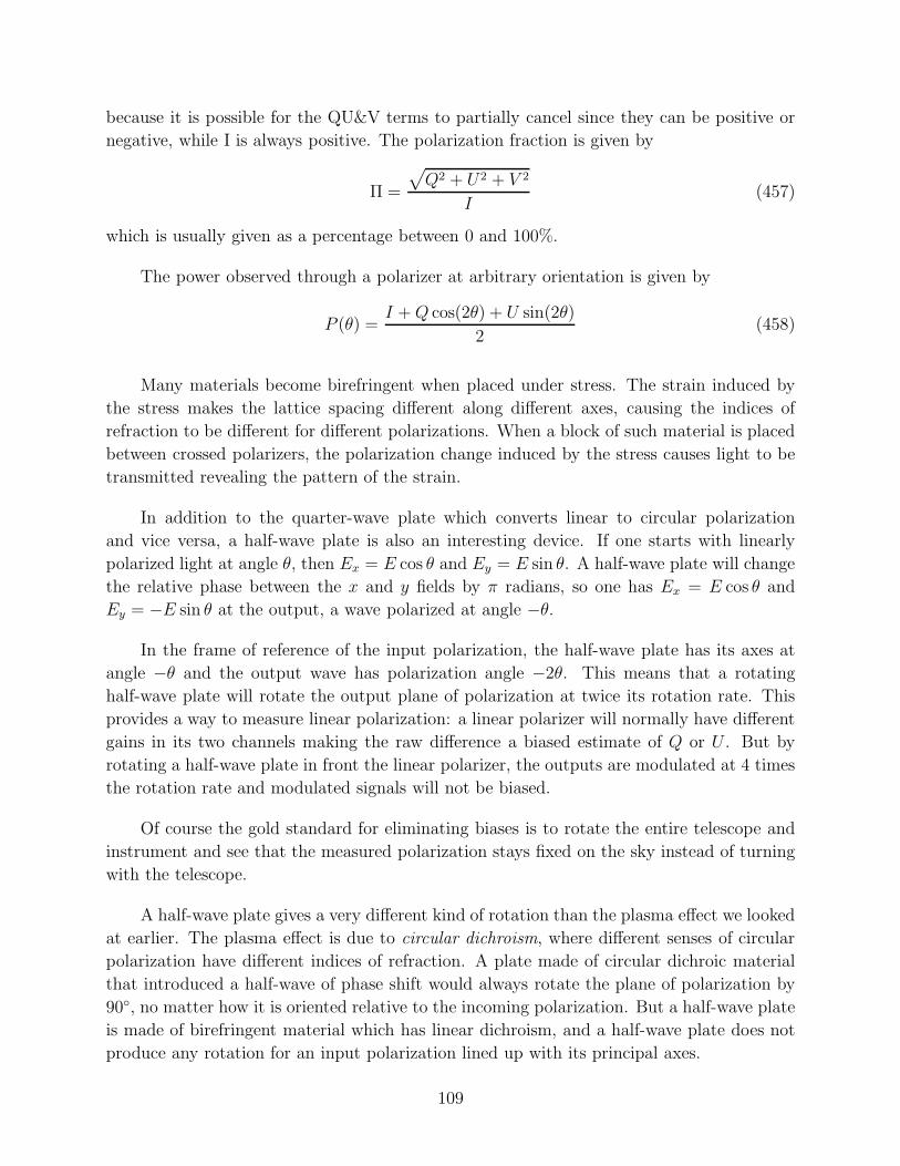
because it is possible for the QU&V terms to partially cancel since they can be positive or

negative, while I is always positive. The polarization fraction is given by

Π =

√

Q2 + U2 + V 2

I(457)

which is usually given as a percentage between 0 and 100%.

The power observed through a polarizer at arbitrary orientation is given by

P (θ) =I +Q cos(2θ) + U sin(2θ)

2(458)

Many materials become birefringent when placed under stress. The strain induced by

the stress makes the lattice spacing different along different axes, causing the indices of

refraction to be different for different polarizations. When a block of such material is placed

between crossed polarizers, the polarization change induced by the stress causes light to be

transmitted revealing the pattern of the strain.

In addition to the quarter-wave plate which converts linear to circular polarization

and vice versa, a half-wave plate is also an interesting device. If one starts with linearly

polarized light at angle θ, then Ex = E cos θ and Ey = E sin θ. A half-wave plate will change

the relative phase between the x and y fields by π radians, so one has Ex = E cos θ and

Ey = −E sin θ at the output, a wave polarized at angle −θ.

In the frame of reference of the input polarization, the half-wave plate has its axes at

angle −θ and the output wave has polarization angle −2θ. This means that a rotating

half-wave plate will rotate the output plane of polarization at twice its rotation rate. This

provides a way to measure linear polarization: a linear polarizer will normally have different

gains in its two channels making the raw difference a biased estimate of Q or U . But by

rotating a half-wave plate in front the linear polarizer, the outputs are modulated at 4 times

the rotation rate and modulated signals will not be biased.

Of course the gold standard for eliminating biases is to rotate the entire telescope and

instrument and see that the measured polarization stays fixed on the sky instead of turning

with the telescope.

A half-wave plate gives a very different kind of rotation than the plasma effect we looked

at earlier. The plasma effect is due to circular dichroism, where different senses of circular

polarization have different indices of refraction. A plate made of circular dichroic material

that introduced a half-wave of phase shift would always rotate the plane of polarization by

90, no matter how it is oriented relative to the incoming polarization. But a half-wave plate

is made of birefringent material which has linear dichroism, and a half-wave plate does not

produce any rotation for an input polarization lined up with its principal axes.

109

Polarizing devices can be used to make some very useful instruments. The FIRAS

spectrometer on COBE, which measured the spectrum of the sky over a factor of 100 in

frequency, used a polarizing Michelson interferometer. The wavelength range was 1 cm to

100 µm, so the polarizers were made using wire grids having a 25 µm spacing and wires 12.5

µm in diameter. These wires were wound over a support frame on a lathe, and then were

soldered to the frame. This gave two layers of wires, so one was cut away, leaving a free

standing wire grid polarizer.

FIRAS used input polarizers to make a polarized beam, then used another polarizer

tilted at 45 to make a 50:50 beamsplitter that worked over a 100:1 range in frequency.

Radiation that reflected off the beamsplitter, went to the end mirror, returned to the beam-

splitter, and then needed to be transmitted. This requires a 90 change in the orientation of

the polarization. This could not be achieved with with a half-wave plate or a circular dichroic

plate because of the very wide range of wavelengths. But a clever arrangement of mirrors

could do the job. When horizontally polarized radiation hits a mirror, the reflected waves

are horizontally polarized. For vertically polarized waves, the reflected waves are vertically

polarized. So a simple mirror will not work. But a two mirror arrangement called a dihedral

will work. This has two mirrors joined at a 90 angle along a vertical axis. A wave polarized

at 45 that hits the dihedral on the right side will hit the top right side of the dihedral,

bounce over to the top left side of the dihedral, and come back polarized at 135. This is

not a rotation, but rather a flip of the polarization angle around the axis of the dihedral.

So in FIRAS, radiation polarized at 45 is transmitted at the beamsplitter, goes down

arm 1, is reflected and flipped in polarization by the dihedral, comes back to the beamsplitter

and is now reflected. Meanwhile radiation polarized at −45 is reflected at the beamsplitter,

goes down arm 2, is reflected and flipped in polarization by the dihedral, comes back to the

beamsplitter and is now transmitted. All the radiation is recombined but with a variable

phase shift of 2(L1 − L2)/λ waves, where L1 and L2 are the lengths of the two arms, so

the FIRAS interferometer is basically a variable wave plate. When the phase shift is an

integral number of waves the linearly polarized input is unchanged at the output. When the

phase shift is a quarter-wave plus an integer the vertically polarized input becomes circularly

polarized at the output. When the phase shift is a half-wave plus an integer the linearly

polarized input is rotated 90 at the output. So the radiation that gets through an output

polarizer is 100%, 50%, 0%, 50% & 100% as the path length difference is changed from 0 to

λ/4, λ/2, 3λ/4 & λ.

Radar astronomers usually transmit circular polarization to avoid problems with the

rotation measure of the Earth’s ionosphere. When circularly polarized radiation is reflected

by a mirror, the rotation of the electric field is still the same but the direction of propagation

is reversed. As a result, the sense of the circular polarization is reversed, so left circular po-

larization becomes right circular polarization and vice versa. But if the radiation is reflected

by needles, the reflected power will be linearly polarized, corresponding to an equal mix of

110

µ0.0 0.2 0.4 0.6 0.8 1.0

0.0

0.1

0.2

0.3

0.4

0.5

0.6

0.7πI

/Flu

x

Ir [horizontal]

Il [vertical]

Fig. 25.— The limb darkening curves in orthogonal polarizations for an electron scatter-

ing plane-parallel atmosphere in radiative equilibirum, from Chandrasekhar (1960, Radiate

Transfer, Dover).

left and right circular polarization. Thus the ratio of circular polarizations in the received

echo is another way to study the nature of the reflecting body. This is called the SC/OC

ratio, for the “same circular” to “opposite circular” ratio. Note that a mirror or specular

reflection gives SC/OC << 1, randomly oriented needles (“chaff”) will give SC/OC = 1,

and a dihedral mirror will give SC/OC > 1.

Note that radar astronomy is limited by the 1/R4 dependence of its signal to noise ratio.

One get an inverse square law for the outgoing pulse and another inverse square law for the

received pulse.

21. Polarized Radiative Transfer

Because the Stokes parameters are additive, it is mathematically reasonable to take

derivatives of the (IQUV ) vector and to operate on this vector with a matrix. Let I represent

the vector of IQUV . Scattering usually produces a polarization, while true absorption and

emission does not. The source function has to be a four-dimensional vector in the Stokes

111

parameter space. There will be a phase matrix P(n, n′) describing how the input polarization

is transformed into the output polarization. Thus

dI(n)

ds= n

∫

dσ

dΩP(n, n′)I(n′)dΩ(n′) + αB − (σ + α)I(n) (459)

where α is the true absorption per unit length, B is the Planck function, and σ is the

scattering per unit length but dσ/dΩ is the differential cross-section.

In a plane-parallel atmosphere, it seems easiest to work out the phase matrix P for a

polarization basis Il and Ir, where Il is polarization in the plane containing the vertical and

the line-of-sight, while Ir is perpendicular to that plane.

The net result for electron scattering is an equation

µ∂

∂τ

(

Il(µ)

Ir(µ)

)

=

(

Il(µ)

Ir(µ)

)

− 38

∫(

2(1− µ2)(1− µ′2) + µ2µ′2 µ2

µ′2 1

)(

Il(µ′)

Ir(µ′)

)

dµ′ (460)

taken from Chandrasekhar (1960, Radiative Transfer, Dover)

Chandrasekhar also solves these equation for the case of a constant flux F coming

from below and no incident radiation. This would be a star in radiative equilibrium with

an electron scattering atmosphere. Figure 25 show the limb darkening curves in the two

polarizations. The fractional polarization is zero at µ = 0 as it must be by symmetry, and

rises to 11.7% at the limb. But the radiation is primarily moving outward at the surface,

the light scattered toward the horizon is primarily horizontally polarized.

22. Albedo and Asteroids

When dealing with planets the albedo or reflectivity is often needed. Two different kinds

of albedo are defined.

The geometric albedo (pV for the V band) is the ratio of the reflected light at phase angle

α = 0 to the light reflected by a white Lambertian disk of the same size. A Lambertian disk

has the same surface brightness at all angles, but because the observed surface area goes

like cosα the amount of reflected light goes down as α increases. Because a Lambertian

disk scatters into several steradians, it is possible to have an object that reflects more light

straight back to the source giving a pV > 1 A cat’s eye is an example of this, or a corner

cube. Bicycle front and rear reflectors do it, as does Scotchlite tape.

The Bond albedo A is the ratio of total reflected light to the total incident light. To get

the total reflected light we need to integrate over phase angles. If the phase function φ(α) is

112

normalized to unity at α = 0 then for a Lambertian disk the integral

∫

φ(α)dΩ = 2π

∫ 1

0

µdµ = π (461)

The phase integral q is defined as

q =1

π

∫

φ(α)dΩ (462)

so it is normalized to unity for a Lambertian disk. The Bond albedo is defined as

A = pq (463)

For a white Lambertian sphere the geometric albedo is given by

p =

∫ π/2

0cos θd(sin2 θ)

∫ π/2

0d(sin2 θ)

=

∫ π/2

02 cos2 θ sin θdθ

1=

∫ 1

0

2µ2dµ =2

3(464)

Note that the projected radius on the sky goes like sin θ where θ is the angle from the sub-

solar point, so d(sin2 θ) is d(Area). Since this is still a white object that reflects all the

incident light, the phase integral for a Lambertian sphere is q = 3/2 so the Bond albedo is

still A = 1. For the white disk, φ(90) = 0, but for the white sphere

φ(90) =2∫ 1

0

√1− x2 xdx

(2/3)π=

∫ 1

0

√1− y dy

(2/3)π=

1

π(465)

The larger φ(90) explains why q = 1.5 > 1 for the white sphere.

The absolute magnitude of an object that is seen by reflected sunlight is defined as the

magnitude it would have if it were 1 AU from the Sun, and 1 AU from the observer, and at

a phase angle α = 0. This is an unlikely situation since it implies the observer is located at

the Sun, but it gives a well-defined geometry. This absolute magnitude is called H , which

should not be confused with the 1.6 µm Johnson magnitude H .

The Minor Planet Center uses a particular parameterized model for the phase function to

convert observed magnitudes into absolute magnitudes. This phase function is parameterized

by a “slope parameter” G:

φ(α) = (1−G)φ1(α) +Gφ2(α)

φ1(α) = exp[−3.33 tan(α/2)0.63]

φ2(α) = exp[−1.87 tan(α/2)1.22] (466)

(467)

Since φ2 declines less steeply with α than φ1, a large G means a shallower slope for the phase

function. The default value for the phase function is G = 0.15. The value for the phase

113

integral is q = 0.29 + 0.684G and the value of the phase function at 90 is φ(α = 90) =

0.0358 + 0.1185G. For the default slope parameter G = 0.15, the phase integral is q = 0.384

and φ(α = 90) = 0.0535. Note that the white Lambertian sphere has a much shallower

phase function (and hence a larger phase integral) than that given by any reasonable value

of G in the range 0 to 1.

With these definitions the absolute magnitude H is related to the observed magnitude

V by

H = V − 5 log10(r∆) + 2.5 log10[φ(α)] (468)

where r is the distance from the Sun, and ∆ is the distance from the observer. The relation-

ship between H and the diameter D of the asteroid is given by

D = (1329 km)10−0.2H/√pV . (469)

For example, the threshold for potentially hazardous asteroids, H < 22, corresponds to

D > 0.14 km for pV = (1329/0.14)210−0.4H = 0.143.

22.1. Thermal Models

Asteroids are generally too small to resolve with a telescope unless the telescope is

the HST and the asteroid is one of the largest. Thus to determine the diameter one must

either assume an albedo or obtain some other data about the asteroid. Observations of the

thermal infrared radiation emitted by the asteroid are very useful for albedo determinations

because the fraction (1−A) of the sunlight that is not scattered is absorbed and reradiated

in the thermal infrared. If one could observe an asteroid from all directions and compute its

“luminosity” in scattered light and infrared reradiation, Lopt and LIR, then the Bond albedo

is determined fromA

1− A =Lopt

LIR. (470)

The diameter would also be well-determined, since

Lopt + LIR = π(D/2)2 L⊙

4πr2. (471)

Of course one usually only observes the asteroid from one angle, and one needs to know the

optical and infrared phase functions to extrapolate from one phase angle to the integral over

all phase angles. Knowing the infrared phase function involves modelling the temperature

distribution on the surface of the asteroid, and several different models are commonly used.

Clearly the simplest possible thermal model is an isothermal asteroid with the same

temperature at all points on the surface. This has a constant infrared phase function, φ = 1

114

for all angles, and thus a phase integral of 4. If the surface of the asteroid radiates like a

greybody with emissivity ǫ then the temperature is given by

ǫσSBT4[4π(D/2)2] =

(1− A)π(D/2)2L⊙

4πr2. (472)

For ǫ = 1 and A = 0, this is T = 279[r/(1 AU)]−1/2 K. The isothermal model is reasonable

for very small asteroids, rapidly spinning asteroids, and for planets with atmospheres which

have a large thermal inertia like the Earth, which explains why 279 K is such a pleasant

temperature. A more detailed model of the Earth would include the albedo, A ≈ 0.24,

which makes the temperature colder, and also the warming due to the greenhouse effect in

the atmosphere, again giving a pleasant surface temperature.

For asteroids larger than tens of meters, conduction is inefficient at transferring heat,

so there is a large temperature gradient around the surface. This is often modelled using the

Near Earth Asteroid Thermal Model (NEATM, Harris, A. W. 1998, Icarus, 131, 291-301),

which assumes that the surface temperature at an angle θ away from the sub-solar point is

given by T (θ) = Tss max(0, cos θ)1/4 where the sub-solar temperature is given by

ǫησSBT4ss =

(1−A)L⊙

4πr2. (473)

The “beaming parameter” η is a fudge factor that can be adjusted to make the model

spectrum match the observed spectrum. The model spectrum for a given phase angle is

obtained by integrating ǫBν(T (θ)) over the observed disk of the asteroid. Note that the

integrated, or bolometric, infrared phase curve of the NEATM is exactly the same as the

phase function of the perfectly diffusing Lambertian sphere. Thus the phase integral is 1.5.

For wavelengths shorter than the peak of the IR spectrum the phase curve will be steeper

and the phase integral smaller, while the reverse is true for wavelengths longer than the

peak.

The NEATM with η 6= 1 does not satisfy radiative equilibrium. Thus the derived value

of η has to vary with viewing angle. When viewing the morning side of a rotating asteroid,

the temperature of the visible parts of the asteroid will be cooler than equilibrium giving a

high η, while in the afternoon the temperature will be warmer leading to a low η. These

variations are due to physical effects that are not included in the NEATM, such as heat

conducted into the surface during the day that is radiated later at night. Thermophysical

models do include such effects.

Another commonly used simple thermal model is the Fast Rotating Model, or FRM. In

this model the Sun is over the equator of a rapidly spinning asteroid. Then the heat input

depends on the latitude θ and local hour angle of the Sun as

F (LHA) = cos θmax[0, cos(LHA)](1−A)L⊙

4πr2(474)

115

which averaged over LHA gives

〈F 〉 =cos θ

π

(1−A)L⊙

4πr2(475)

This leads to a temperature on the equator that corresponds to the sub-solar temperature

of the NEATM with η = π. But the phase function for the FRM is a constant when the

observer is over the equator. This is the usual assumption. When the observer is over the

pole at α = 90 the phase function is smaller. The phase integral integrated over solid angle

is high so the FRM is in radiative equilibrium. The day side is cooler, but the night side is

just as hot as the day side.

All of these simple models assume a spherical asteroid. The infrared flux is found by

integrating over the observed disk of the asteroid. For the NEATM at 0 phase angle the

flux is

Fν =(D/2)2

∆2ǫ

∫ 1

0

Bν(Tss[1− x2]1/8)2πxdx (476)

where x is the normalized radius on the observed disk, which is sin θ if θ is the angle from

the sub-solar point.

For the NEATM at 90 phase angle, the flux is

Fν =(D/2)2

∆2ǫ

∫ 1

0

Bν(Tssx1/4)4√

1− x2dx (477)

where now x = cos θ is the normalized x coordinate on the disk.

For the FRM seen equator-on, the flux for any phase angle is

Fν =(D/2)2

∆2ǫ

∫ 1

0

Bν(Tss[1− y2]1/8)4√

1− y2dy (478)

where y is the sine of the latitude.

Finally for the FRM seen pole-on, at 90 phase angle with a particular clock angle, the

flux is

Fν =(D/2)2

∆2ǫ

∫ 1

0

Bν(Tssx1/4)2πxdx (479)

where x is now the cosine of the latitude which is the normalized radius on the disk.

c©Edward L. Wright, 2016

116