Astronomy 480 - IRAF Tutorial 1 Starting IRAF. This is a short exercise that should help acquaint you with the basics of IRAF. The first step is to get IRAF running properly, with appropriate auxiliary windows. 1.cd to your IRAF home directory. 2.Start a new window by typing xgterm & at the Linux prompt on your machine. 3.Start up an DS9 window by typing ds9 & in the xgterm window. 4.Now start up IRAF by typing cl Hint: It is important that you initiate IRAF like this, from within an xgterm window. If you find at some stage that a stream of unintelligible garbage is spewing at your IRAF session, you probably started IRAF from a regular xterm/KDE shell window. Also, be sure you start IRAF from the directory that contains the IRAF initialization file, login.cl. The xgterm is set up to interpret graphical information, and to open up a graphical (i.e. plot) window as appropriate. This will give you the IRAF prompt cl>. In this, as in forthcoming exercises, the boldface commands after the prompt (either % or cl>) are meant to be typed by the user; the #-sign indicates a comment. You can pass commands on to the Linux operating system by prefacing them with a “!”, for example try this cl> !more login.cl which will run the Linux process “more” on the file called login.cl. You can move down by hitting the spacebar, just as in Linux. Notice that there are a number of initialization parameters that take effect when you start up IRAF. IRAF’s heritage is complicated, and much of the syntax was initially like an antique operating system called VMS. There are many instances, however, when the intrinsic IRAF command is identical to the Linux one. For example cl> !ls and cl>ls have the same effect, but you should think of the former as being passed up to the Linux operating system while the second is being carried out within IRAF. File Transfer for this Exercise – (You should already have the images in a directory called exercise1. We are going to move these files to your image directory, and do it within IRAF.) In order to speed transfer over a network and minimize disk space, image files are often stored in a compressed format, that preserves all the information but reduces the file size. From within IRAF, let’s move your test images into a working directory and uncompress them. A typical suffix for compressed files is .gz. Hint: Since images proliferate rapidly, it’s important to use the directory structure to help with organization and bookkeeping. Here’s one way to accomplish a move of images. Don’t do this example, there is a better way (if you’ve been following directions all along! This one is just for added information. cl>cd imdir # move to your images directory cl>ls #list the contents cl>!mkdir exercise1 #create a directory for this exercise within your images subdirectory cl> cd exercise1 # this works as an IRAF command too. cl>!mv ../../exercise1/*.gz . # copy compressed images to the current directory Your files probably resided in /net/projects/Astro_480/spring-05/yourusername/exercise1/ and you should now be in /net/projects/Astro_480/spring-05/yourusername/images/exercise1/ -- make sure you understand the movement between directories in a relative sense! Having said this, there is a much more efficient way to do the same exact thing.

THIS IS THE ONE YOU DO! You should be the same directory in which you started IRAF for this transfer of files (saving you many key strokes at the start): /net/projects/Astro_480/spring-05/yourusername/ Now, type the following from within IRAF: cl>pwd ; ls #check where you are and list the directory contents cl>mv exercise1 images #create a directory for this exercise within your images subdirectory cl>cd images # this works as an IRAF command too. cl>ls # see the subdirectory exercise1? Wondering if the files actually # were transferred as well? You can do either of the following: cl>ls exercise1 or cl>cd exercise1 ; ls -l cl>!gunzip *.gz #uncompress the image files with the “gunzip” utility cl>ls –l > after cl> page after #is the listing of the uncompressed files there? There should be some images called photo1.fits, photo2.fits and photo3.fits in your images directory. If they aren’t there, copy the file photos.tar.gz over from /net/projects/Astro_480/spring-05/larson/images/exercise1/ and extract them. Image Headers The next step is to familiarize yourself a bit with some of the basic operations of IRAF. Tasks with similar/related functionality are grouped together in “packages”. Tasks, and sometimes packages, have parameter files that control their operation. Your login.cl file determines which packages are loaded when IRAF starts. Others must be invoked by loading them as needed. Hint: If you type a favorite IRAF command that it does not recognize, the package is probably not loaded. The image data files we will be using contain both “header” information and digital data. The header information in FITS format files is stored as ASCII characters at the top of the file. You can actually peek at the header of a FITS file in Linux using the “head” command, but it’s not recommended. IRAF has a suite of tools to look at and edit header information. Try this to get started: cl> package # show what packages are currently loaded cl> help images # help for the package "images" cl> phelp imheader # help for task "imheader" - is the proper package loaded for its execution? phelp in IRAF acts like “more” in Linux: <space bar> # go to next page of help b # go back one page ? # view options q # quit the help for this task LPAR (list parameters) Tasks in IRAF usually use parameters that modify the actions taken. These parameters are stored in parameter files in your uparm directory (a subdirectory off your IRAF home directory). To list the values of the parameters you use the utility lpar. It’s common to modify the values of these parameters when running IRAF. In order to revert to the default parameter set, you use the task unlearn. To list the settings of the set of parameters for the task imheader, you would type cl> lpar imheader # list task parameters - task names

Parameters need only enough characters specified to be identifiable, so try cl> lpar imhea cl> lpar imh # this is not unique, more than one task name starts this way….so again do cl> lpar imheader # note query and hidden parameters - query parameters are listed #first with hidden parameters following in parentheses cl> unlearn imhead # unlearn parameters - go back to defaults cl> imhead *.fits # short header listing - what does it tell you? cl> imhead *.fits > shortheads # redirection works! Useful! cl> page shortheads # the “page” task is the IRAF equivalent of “more” in Linux., as in “phelp” above. cl> lpar imhead # this lists the parameters of the task “imhead”… How do you change them? cl> epar imhead # modify the task so it always types the long header listing – Move using the arrow keys, # and then type yes over the parameter entry for "longheader" followed by a #return. It replaces previous text. :wq or <ctrl-D> # exit eparam mode and "save" the new parameters [exiting with <crtl-C> or ZZ does NOT update the parameter file} cl> lpar imhead # was the edited parameter saved? cl> imhead *.fits | page # you should get a long listing by default, now. This last command uses the “pipe” command, “|”, which sends the output stream to another task, as opposed to “>” , the redirection symbol that is used to send the output stream to a file. Be sure you understand the difference. The settings of the IRAF task parameters are stored in the “uparm” directory, off your IRAF home directory. The names are concatenations of the package name, and the task name. Don’t worry, there is a way to always return to the default parameters for any given task: cl> unlearn imhead # go back to the default parameter setting Do a quick self-review about parameters. How do you revert to the default parameters for a given task? What is the uparm directory? Do you understand the different syntaxes that we have been using in task executions? If you have questions see the Beginner's Guide mentioned below in the References section. Besides the course CD, you can access it from the course web site, http://www.astro.washington.edu/astro480. History IRAF can redirect terminal output to a file, as well as pipe output from one task into the input of another task. There is also a history and recall mechanism. cl> history # prints history tree cl> ^ # recall and execute last command, can also include number to execute any task in tree cl> ehis lpar # recall last lpar command - allows you to edit command line before executing with "return" - # use the arrow keys to move cursor, delete or insert to the left of the cursor cl> e (=ehis) # recall last command - use up/down arrows to go up/down history tree, and edit, executed just #like in Linux shell cl> history 100 # look at last 100 commands cl> history 100 > hfile # redirect output to a file cl> page hfile # page the file cl> history 100 | page # alternate method avoiding intermediate file Note the difference between ">" and "|".

Some Applications The images that now reside in /net/projects/Astro_480/spring-05/yourusername/images/exercise1/ are frames obtained in testing candidate replacement detectors for a mosaic CCD camera. Let’s take a look and then display one of them. cl> ls *.fits cl> imstat *.fits #prints out summary table with useful info. Try listing its parameters. cl> unlearn display cl> set stdimage=imt6 # configures image display to accept large format images; temporarily overrides # the default we typed into login.cl file. cl> lpar display # look at the parameters for the display task cl> display test-f1 1 # load the first image into the image display You should see a rectangular CCD image on the ximtool display, as well a smaller image with the full image shown in the upper right corner of the ximtool window. DS9 – An image display tool. Let us digress for a moment. This is probably a good time to acquaint yourself with DS9. This utility allows you to view image data as a greyscale image. The correspondence between the raw data values and the shading on the screen can be controlled, to bring up features near the background level for example. You can also “zoom” in on regions of interest. DS9 will handle a stack of images at once, placing each one in a distinct “buffer” that is referenced by numbers. You should already have DS9 running, and you should learn how to zoom, pan, window, and blink between multiple images. All these options can be done with the mouse. Notice the pull down menus at the top of the window. Pull each menu down and review the selections - use the left mouse button to activate and pull down the menus. Take some time to browse the help pages for DS9, although they’re somewhat terse! You can access the reference manual through the button in the top right corner of the window. The greyscale lookup table can be modified by moving the cursor up and down in the window (contrast) or left and right (brightness) while holding down the right mouse button. The bar across the bottom of the DS9 window shows how the digital data values are mapped onto the displayed greyscale. If the bar across the bottom shows only the far right end as white, and the rest as black, then only the highest data values will be displayed as white, and the rest black. Alternatively, if the entire bar across the bottom is the same grey color, then all pixel data values will show up as that same grey (contrast = 0). Watch the brightness and contrast values in the Control Panel box as you hold down the right mouse button and move the cursor around the frame.

See if you can find a greyscale setting that brings out the texture in the main image section of the frame (i.e. not the overscan).

Panning and zooming are done with the middle mouse button. Move the cursor to an interesting part of the image - click twice with the middle mouse button without moving the cursor. Click again without moving the cursor. If you move the cursor and then click, the region under the cursor is moved to the center of the window (panning). If you click without moving the cursor then the region is zoomed. Play with this until you understand how it works. Go back to the unzoomed image when you are finished.

We want to blink this field and that of test-f1. So we will need to load the second image into the second frame buffer - you have 4 frame buffers available for images. Let’s load an image into buffer #2:

cl> display test-f2 2 Blink between the two frames by pressing the “Frame” and then "Blink" buttons – you can adjust the blink rate if you wish, by using the drop down “Frame” menu. These two routes, oferring simple and more complex options respectively apply to most controls in DS9. Do you see small differences between the frame? You may have to zoom in on a small region to see the subtle differences in pixel values. Play a bit with DS9 until you feel comfortable with it.

Now, let’s display some different images:

cl> display photo2 3 cl> disp photo3 4

Scroll through the 4 frames using the “Frame” button options (i.e. next/previous) . Notice that the name of the image changes, at the top of the window, as you change what is displayed. Imexamine Recall that a FITS file contains the header information, and a 2-dimensional (usually, anyway) array of intensity values corresponding to the amount of light detected at each pixel. With an image displayed on the DS9 window, you can use one of IRAF’s most powerful interactive utilities to explore the pixel data. In the IRAF window, type cl> imexamine This provides access to a toolkit that will take some time to explore. The cursor appears as a small round doughnut. Keystrokes initiate a number of tasks that occur centered on the cursor. Here is a list of some imexamine tasks you should try out: ? lists imexamine options z prints out pixel values in a region around the cursor m computes statistics on pixels near the cursor s makes a surface plot of the region around the cursor e makes a contour plot of the region around the cursor l makes a plot of the pixel values of the line containing the cursor c makes a plot of the pixel values down the column that contains the cursor q quits out of imexamine task, control returns to IRAF xgterm window Try these out and see what happens. Place the cursor over a stellar image in the photo2.fits image, and try z, s, e, and r in imexamine. Refer to the on-line phelp facility for imexamine, as needed. While you’re running imexamine you can change how IRAF interprets keyboard and mouse inputs. You can switch between the original IRAF session, the DS9 window and the graphics window (the one that displays graphs). The table below describes how to change the input mode between the IRAF xgterm, the “graphics” window (the gterm with the plots) and the “image” window (DS9). If you close the graphics window while running imexamine, you will not be able to reopen it without restarting imexamine.

To go to Type IRAF window q

Image cursor i

Graphics cursor g Table I. Keystrokes to switch input streams in imexamine

Make sure you feel comfortable with imexamine. We will use it almost every day for the rest of the quarter. With the image test-f2.fits displayed on the DS9 window, use imexamine and the graphical and image display windows to roam around the frame. In this image the output amplifier is at the lower left corner of the picture, at pixel 1,1. cl> display test-f2.fits 1 #puts image into DS9 buffer 1 cl> imexamine

Now execute the following keystrokes, with the cursor positioned somewhere in the middle of the image: l #the letter ‘l’ produces a plot of the line under the cursor g #changes cursor over to the graphics window. Move the mouse over that frame :y 200 3000 #rescales the y-axis of the plot to range only between 200 and 5000 :x 1020 1050 #zooms in on columns towards the right edge of the detector Can you tell where the overscan pixels begin? Hint: You can generate a hardcopy printout of whatever is in the graphics window by first entering the graphics cursor mode, then hitting the (equal) key. The line on the bottom of the graphics window will say “.snap - done”. The plot will appear on your default printer (probably Goddess in UAI-B356!). You can generate a postscript file printable with the usual Linux lpr command. First, epar stdplot, and change “devices” to “epsl”. Then from the graphics window issue the command :write plotname. Lastly run stdplot plotname and a file with .eps should appear in the directory- the postcript file. You should now be able to work through the appended worksheet. Refer to the online “phelp” facility and this document before asking for help. If those don’t work, then by all means ask your instructor or one of your fellow students. When you’ve filled out the appended worksheet, hand it in and exit IRAF by typing cl> logout References A Beginner's Guide to Using IRAF, by Jeannette Barnes, August 1993. On-line IRAF tutorial materials, on which this is based.

Name:__________________________________________________________________ Date:______________ Due: IRAF – EXERCISE 1 These questions refer to the image /exercise1/test-f2.fits -- be sure that is the image you have displayed! Part I 1. Where was this image taken, with what size of a telescope, and with what instrument and detector? 2. On what date was the observation made? How long was the exposure? 3.How many rows are there in the image? ____________ How many rows are there in the frame? ____________ 4.How many columns are there in the image? ____________ How many columns are there in the frame? ____________ 5.What is the first pixel that is read out? Which is the last pixel? (Look at the DS9 cursor information! Use imexmaine’s “z”

option, perhaps…?) The convention is to label pixels by [column (x), row (y)] coordinates. First one read out: ___________ Last one read out: ___________ 4. How many pixels are there in the entire image? This is inconsistent with what you saw for Npix in “imstat” earlier. Why? 5 There are “overscan” pixels in this frame, which were never exposed to light during the exposure. How many overscan pixels are at the end of each row? How many overscan rows occupy the top of the image? Overscan pixels per row: __________ Overscan rows: __________ Part II 6.Hmm….The electronics for this camera uses a 16 bit Analog to Digital converter. If 216=65,536 then why does imstat

report the highest pixel value as being 65,535? 7.Is there a region on this detector where the charge is “smeared” out due to poor charge transfer efficiency? If so, what

general region is afflicted the worst? 8.Use the “m” facility in imexamine to measure the standard deviation that characterizes the overscan region. Poke around

and estimate a value to 2 significant figures. This is a reasonable first estimate of the “noise” that competes with the measurement of small amounts of charge.

a. Is the noise the same in the overscan on the edge and across the top of the frame? How do the noise levels compare? b. What are the units attached to this noise figure?

9.The average value in the overscan region is called the ‘bias” level. Use the “c” and “l” utilities in imexamine to determine

how much the bias value varies in the overscan region. Do you think it could be subtracted as a simple scalar value from the entire array, or should it be determined and subtracted row by row? Explain.

10.You can get a sense of the charge transfer efficiency (CTE) by looking at how rapidly the intensity falls in the overscan

region. On this particular detector, is the parallel (between rows) or serial (between columns) CTE better? Why?

ASTRO 480- IRAF TUTORIAL 2

Quick-look Photometry with Imexamine Introduction One of the most basic astronomical measurements involves determining the flux from an object, over a particular range in wavelength (“passband”), that is intercepted by the detector. The process of extracting flux measurements from images is called photometry. As you will see below, photometry is by no means trivial. Two of the major challenges are 1) compensating for the absorption of light by the atmosphere (extinction) and 2) eliminating unwanted light from sources other than the object of interest. Magnitudes By convention, astronomical fluxes are measured in magnitudes. We need to first distinguish between “absolute” and “apparent” magnitudes. Apparent magnitudes are simply a measure of how much light gets to the Earth from a celestial object, and are represented with a lower-case letter, such as m = 12. This is determined both by the object’s intrinsic luminosity, by how far away it is, and how much stuff may be in between us and it that could block some of the light. The “absolute” magnitude of an object, on the other hand, refers only to its intrinsic luminosity, and is usually represented with an upper-case letter, M = 8 , for example. This is usually tough to determine since you need a reliable way to establish the object’s distance. The measurement of line-of-sight distance is the one of the biggest challenges that astronomers face. Magnitudes are a logarithmic scale. Two objects that differ in measured flux by a factor of 100 are defined as having 5 magnitudes difference. The fainter of the two objects is assigned the larger magnitude value, i.e. an object of 18th magnitude is 100 times fainter than an object of 13th magnitude. The apparent magnitude difference between 2 objects is then given by

!

m1 "m2 = "2.5log10f1

f2

#

$ %

&

' ( ,

where m1 and m2 the magnitudes, and f1 and f2 are the observed photon fluxes. With the determination of the slope of the magnitude scale given by the definition above, there is an arbitrary constant that determines the “zeropoint” of any given photometric system. Traditionally, this has been defined by using the star Vega as the definition of 0th magnitude. This traces it roots to early attempts by the Greeks to classify stars according to their apparent brightness. First magnitude stars were supposed to be twice as bright as second magnitude stars, etc. The human eye is close to a logarithmic detector, and the contemporary magnitude scale still retains much of its historical heritage. Given the wide range in brightness spanned by astronomical objects, a logarithmic scale makes a lot of sense. The apparent magnitude of the Sun is about –27, the full moon is –12.5, and you can barely pick out stars as faint as 6th magnitude with the naked eye. The faintest objects observed with HST or ground-based telescopes are at around 30th magnitude. For any given telescope, filter and detector system, the apparent brightness of an object, expressed in apparent magnitudes, is given by

!

m = "2.5log10( f ) + m0 where the constant m0 (the “zeropoint”) is determined by measuring the flux for “standard” stars that serve as calibrators. This zeropoint in magnitude is the single scaling factor for an astronomical

imaging system. You can measure the flux in A/D converter units (“ADUs”) per second, plug those values into the formula above, and sweep all the calibration factors into the system’s zeropoint. If done this way, the zeropoint represents the magnitude of an object that would produce a detected signal accumulation of 1 ADU per second. Astronomers often refer to “instrumental magnitudes,” where the value of m0 is not tied to a well-defined set of standards. This is perfectly fine as long as one is only interested in relative fluxes between measured objects. It’s important to make clear, however, whether one is referring to instrumental or calibrated magnitudes. Atmospheric Extinction The magnitude scale is defined as flux that is incident at the top of the atmosphere, as if the measurements were being carried out by an ideal telescope in orbit above the Earth. This will require that we correct for the (wavelength-dependent) absorption of light by the atmosphere. The determination of these extinction corrections requires taking a set of observations that are specifically used to establish the values of the extinction correction parameters. One way to do this is to measure the apparent flux from a stable star at a variety of zenith angles, and make a plot of the flux vs. the amount of atmosphere along the line of sight. You then determine the flux extrapolated to zero atmospheres, i.e. an airmass of zero. Since the determination of atmospheric extinction requires a succession of measurements over time, the properties of the atmosphere must remain stable over that period. When the atmosphere is stable and flux depends only on airmass (and not on time) the conditions are considered to be “photometric,” i.e. adequate for making photometric measurements. In contrast, when it’s partially cloudy astronomers call the conditions “spectroscopic.” In practice, establishing whether the conditions are photometric is not trivial, since it’s pretty hard to see clouds at night, especially high cirrus (the bain of observational astronomers)! There are 3 ways (that we know of) that are used to determine whether conditions are photometric: 1.Check for any clouds at sunset and sunrise. If none are seen then assume it was clear all night. 2.Check to see if the photometry results have scatter that is consistent with Poisson noise, with no

excess scatter. 3.Use an infrared camera to monitor the sky. Clouds are nicely visible at a wavelength of 10 microns. This last technique is very effective. There is a 10 micron all-sky cloud camera in use at the Apache Point Observatory, and you can look at the results by going to the APO web site, http://www.apo.nmsu.edu, and moving to the link labeled “weather conditions.” Sky Subtraction One complication in doing photometry is that the object of interest is superimposed on flux from the sky. This light comes from a variety of sources, including unresolved stars and galaxies, sunlight scattered into the beam (particularly from the moon!), stray light bouncing around in the telescope, and light from manmade sources. A simple model for the sky is to assume it’s uniform, at least in the immediate vicinity of the object of interest. The sky brightness is then given in magnitudes per square arc second. The sky brightness depends on the wavelength under consideration, as well as the phase of the moon. Typical values at a dark site are ~20th mag per square arc second. The flux from the sky is

then equal to what you would see if a 20th magnitude star were placed in each square arcsecond of the sky, except of course the sky flux is uniform. If you think of the flux from the object of interest as sitting on top of flux from the sky, then clearly we’d like to move away from the star, measure the sky background, and then subtract the sky level from the pixels that contain the object’s flux. This process is called “sky subtraction.” In very crowded fields it is often hard to get a good measure of the sky brightness, and this is a major source of systematic error. A common technique for determining the sky level is to specify an annulus around the star, and compute the mode or median (debates rage!) of the intensity in the annulus. This value is then subtracted from the pixels that contain the object of interest. A slightly more sophisticated mechanism uses a tilted plane model for the sky, fitting to the I(x,y) intensity values in the sky annulus, and uses this model to subtract the sky. This allows for first order gradients in the sky brightness. It is usually best to determine the sky value locally for each object of interest, rather than applying a single value to an entire frame. PSF-Fitting vs. Aperture Photometry When the light from an astronomical point source is brought to a focus at the focal plane of a telescope, ideally we would see a diffraction-limited image, with Airy rings. In reality both the atmosphere and the telescope optics (especially poor focus) degrade the image, to something that is more like a 2-dimensional Gaussian profile. The 2-d function that describes the light distribution in the focal plane that comes from a point source is called the Point Spread Function, or PSF. Clearly, the integral of the flux “under” the PSF is proportional to the flux received from the source. There are two common techniques to measure the flux of an object of interest; PSF-fitting and aperture photometry. Aperture photometry is the simplest to understand: just place a circular aperture around the star of interest and add up the flux from the object that is within the aperture. This works well if the stars are well separated, so that only the flux from a single object appears in the aperture. The choice of aperture size depends on the objective of the program. If you’re just interested in the relative fluxes of objects in the image, then (as long as the stellar images are the same everywhere) the result is independent of aperture size. On the other hand, if you’re interested in doing an absolute measurement (i.e. count every photon!) then the typical approach is to do aperture photometry for a sequence of apertures, and fit the (increasing) measured flux as a function of aperture size. The asymptotic value at Raperature = ∞ is the best estimate of the total flux from the object. This is called a “curve of growth” analysis. For crowded fields aperture photometry does not work very well. The stellar images blend together, and any given pixel might contain flux from multiple objects. In this case we try to first establish the shape of the stellar image, or Point Spread Function (PSF) from a bright, isolated star. The flux in an object of interest is then determined by fitting the image data to a model of the PSF. Even in PSF-fitting photometry, there are choices to be made. Should the stars be fitted individually, or simultaneously? Is it better to use a mathematical model of the PSF, or to retain the details of the empirical PSF? There are two programs that are in common usage to perform PSF-fitting photometry: DAOphot (which is bundled within IRAF) and DoPhot (a standalone program).

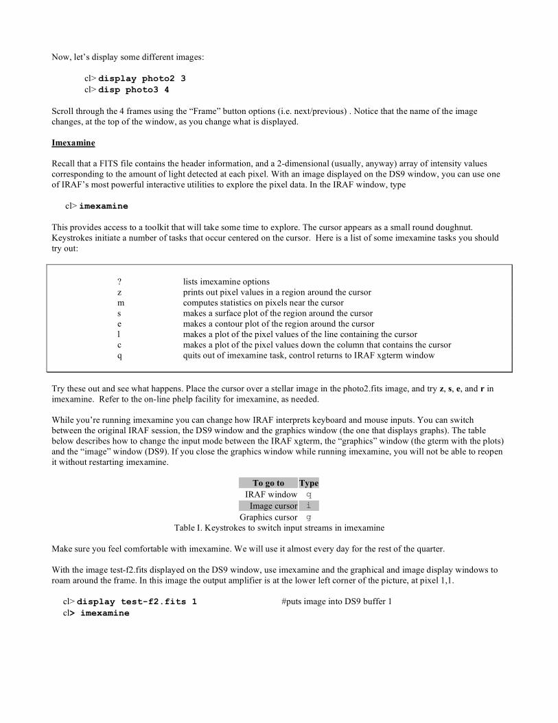
Imexamine photometry, and sky subtraction It is often useful to do quick-look photometry while taking data. The IRAF task imexamine is a very powerful way to do this. You can do sky-subtracted radial fits to stars, using parameters that you can set as desired, and IRAF will make initial estimates of the flux using radial integrals. I strongly suggest you use phelp imexamine to learn how the sky subtraction and quick-look photometry functions work. Concentrate on the sections that deal with the “a” and “r” commands. Notice that the “r” task does aperture photometry, and also plots PSF fits using either Gaussian or Moffat models. The images you’ll need for this exercise are in /net/projects/Astro_480/spring-05/larson/images/exercise2. You should make a subdirectory within the images directory titled (appropriately) exercise2. Go ahead and copy m92.tar.gz over into your image/exercise2 subdirectory, /net/projects/Astro_480/spring-05/username/images/exercise2. Gunzip this file and extract the individual files from the tarball. The IRAF task imexmaine can be also used to illustrate the issue of background (or sky) subtraction. Bring up one of the images of m92 in IRAF, using ds9. Choose two stars that are well separated from any others, and use imexamine to investigate them. First use “s” to make a surface plot of the light distribution: cl> display m920004.fits 1 cl> imexamine cl> s #This shows a picture of the PSF of the star. Now use the “r” function to make a radial plot of the object. This task will also compute the FWHM, the radial integral of the flux, and a sky value. The “r” task produces a number of interesting quantities that pertain to the object of interest. Notice that the pixel values of the centroid of the object appear in the title section of the graphics window, with a resolution much better than an integer pixel value. Also, along the bottom of the graphics window, in the yellow band, appears a line of numbers. These are all described in the on-line help documentation for the imexamine task. If you look at the section around line 630 in the imexamine documentation (do phelp imexamine) you can see the quantities that are produced. (The “r” task in imexamine does nearly the same thing as the “a” task.) Along the top of the graphics window are the centroid x and y (in pixels). Across the bottom of the graphics widow it gives: The object radius used for aperture photometry The object’s magnitude The total flux, in A/D units The mean sky background, in A/D units The peak value of the PSF fit The ellipticity of the object (round has e= 0) The “position angle” of the ellipse, i.e. its orientation, in degrees (aligned with x axis =0) If a Moffatt function is used to describe the PSF, a parameter Beta of that function is given next Then come 3 different estimates of the FWHM (Full Width at Half Maximum) of the PSF. The last one of these is probably the best one to use, as it uses the data alone and does not depend on model fitting.

Do “r” for a few stars, in the m920004 frame. Compare the task’s output with the listing given above. Are the centroids sensible? Is the FWHM sensible (the units are pixels)? Now quit imexamine (for the moment) and list the parameters you’ve been using, with cl> lpar rimexam cl> epar rimexam The sky background is determined from 3 parameters, “radius,” “buffer” and “width.” You should think of 3 concentric circles, centered on the star. The parameter “object radius” is the radius of the first circle, which is used to compute the object flux, with aperture photometry. Then comes an annular buffer with a radius given by “Background buffer width,” followed by an annular region in which the sky value will be computed. The radial size of the background region is given by “Background width.” These parameters can all be modified, with epar rimexam. We’ll do this in a moment. Imexamine is a little too clever for us, though. It will automatically modify the radii it uses, based on the FWHM of the stellar image, unless we insist that it not do so. This is controlled by the “iterations” parameter. Modify the values for rimexam so they match the following list: (banner = yes) Standard banner (title = ) Title (xlabel = Radius) X-axis label (ylabel = Pixel Value) Y-axis label (fitplot= yes) Overplot profile fit? (fittype= moffat) Profile type to fit (center = yes) Center object in aperture? (backgro= yes) Fit and subtract background? (radius = 2.) Object radius (buffer = 0.) Background buffer width (width = 1.) Background width (iterati= 1) Number of radius adjustment iterations (xorder = 0) Background x order (yorder = 0) Background y order (magzero= 25.) Magnitude zero point (beta = INDEF) Moffat beta parameter (rplot = 8.) Plotting radius (x1 = INDEF) X-axis window limit Change the values of the radius and sky subtraction parameters and see how they affect the photometry of the two stars you’ve chosen. The radius is also the aperture used for this implementation of aperture photometry. In particular, try setting the radius equal to one half of the FWHM, with buffer=0. This will then compute sky from a “contaminated” region, and using “r” will show a sky baseline that is clearly wrong. Play around with this some, enough to get the sense for the process of sky subtraction. Note that you can store the results of imexmaine in a logfile. Do “epar imexamine” to turn on the logging feature. Take a look at some other frames and get a feel for the imexamine tool.

References On-line help within IRAF Howell, Handbook of CCD Astronomy, Chapter 5.

A User’s Guide to Stellar CCD Photometry with IRAF, by Philip Massey and Lindsey E. Davis, April 1992.

A User’s Guide to the IRAF Apphot Package, by Lindsey Elspeth Davis, May 1989. Specifications for the Aperture Photometry Package, Lindsey Davis, October 1987.

An aside- Distance Modulus Although the notion of the magnitude scale takes some getting used to, it is in fact a very useful and practical scheme for expressing fluxes. Magnitude differences are a logarithmic expression of flux ratios. The difference of magnitudes in different optical passbands is then a measure of the spectral energy distribution of objects. Magnitudes are also used as a way to express distances. The absolute magnitude of an object is defined as the apparent magnitude you’d see if it were a distance of 10 parsecs way. The distances to more remote objects can then be given as a “distance modulus,” which is simply an expression of how much a stable star’s apparent magnitude would change if it were translated from a distance of 10 pc to the location of the object in question.. For example, the Large Magellanic Cloud, one of our near neighbor galaxies, lies at a distance modulus of D = 18.5 mag. If an object with an absolute magnitude of 3 were moved from a distance of 10 pc away to the LMC, it would have an apparent magnitude of 3 + 18.5 = 21.5. In general, since flux scales like 1/r2, the distance modulus is given by

!

m "M = "2.5log10

f (r)

f (10 pc)

#

$ %

&

' ( = "2.5log10

r

10 pc

#

$ %

&

' (

"2

= 5log10

r

10 pc

#

$ %

&

' ( .

Name:____________________________________________ Date:____________

IRAF Exercise 2, Worksheet.

There is an image called “spicamfocus.fits.gz” in the directory /net/projects/Astro_480/spring-05/larson/images/exercise2/, which you should copy over. It’s a typical focus frame, taken with an instrument called SPIcam on the Apache Point 3.5 meter telescope. Each pixel in the image spans 0.28 arcseconds on the sky. The picture contains multiple images of each star, each at a different focus setting. This is accomplished by doing 5 iterations of 1) open the shutter for 10 sec, 2) close the shutter, 3) shift the charge on the detector down by a few rows, 4) change the telescope focus, 5) repeat. The CCD is then read out. To keep track of things there is a double-skip in the charge transfer on the last iteration. For this frame, assume the focus was set to (1100, 1200, 1300, 1400, 1500) microns with the 1500 micron setting corresponding to the images that are “double-spaced.” 1) By how many rows is the image shifted between focus settings? (The single-space shift) ________ 2) When the telescope has its best focus, the images should be axisymmetric (ellipticity = 0), smallest (min FWHM), and highest peak intensity (peak at a max). Ideally these would all occur at the same focus setting, but that is not always the case. Check out the faint star whose 3rd image is at (693, 470). Notice that the 3rd image seems better than the rest. This is a clue that the best focus setting will likely be around 1300 microns, but let’s do it quantitatively. Edit the “rimexam” parameter file so that the object radius=4, background buffer width=2 and background width=1. Now choose two well-behaved (unsaturated and isolated) stars and fill in the tables below. Star 1 Double-skip centroid: x= y= (pixels)

Focus Setting Peak Flux Ellipticity FWHM (pixels) FWHM (arcsec) 1100 1200 1300 1400 1500

Star 2 Double-skip centroid: x= y= (pixels)

Focus Setting Peak Flux Ellipticity FWHM (pixels) FWHM (arcsec) 1100 1200 1300 1400 1500

3) What would you choose as the best focus setting for the telescope? On what basis? Which FWHM value did you use?

4) Just using the ds9 pixel readout (accessed from the Analysis menu), what would you estimate as the background sky value for this image, in A/D units? ______________ 5) Let’s investigate how the rimexam parameters affect the results you obtain.for aperture photometry. The settings of the object radius, buffer width, and background width will affect the determination of the sky values and object flux. Edit the rimexam parameter file and set rplot=15 (note – this is not the aperture radius), buffer=1, width=1. For the values of Object radius given, fill in the table below. As you fill in the Table, notice how the sky value in the radial plot varies. Use the isolated star at (523,497) that is in focus. (radius = 1.) Object radius #change this value

For Object at x= 523 y= 497

Object radius Magnitude Flux Sky Peak FWHM 1 2 3 4 8 12 16

6) From your data in the table above, explain how the sky, peak and FWHM values depend on the object radius. Roughly graph the magnitude and FWHM vs radius values in the table below (use different colors or symbols). Do they tend to asymptotic values as the object radius gets larger? Explain. 7) If the “right” answer is obtained with a very large object radius, what disadvantages might dissuade you from using an object radius of, say, 25 pixels?

4_ 3_ 2_ 1_ 0_

1/ 2/ 3/ 4/ 8/ 12/ 16/

_12 _13 _14 _15 _16

ASTRO 480- IRAF TUTORIAL Exercise 3. Image Processing: Bias Frames and Flatfielding

An Introduction to Flatfielding Although CCDs have revolutionized astronomy, they aren’t perfect. Each individual pixel in a CCD array can be thought of as a device that linearly converts light to charge, q, so that for an integration time t,

q A t I QE d B D ti i i i i i= + +! ( ) ( )" " "

where Ai and Bi are the “gain” and “offset” parameters that characterize the pixel i , Ii(λ) is the incident light flux and QEi(λ) is the pixel’s efficiency, integrated over some passband that is usually defined by an optical filter. There is also some thermally generated “dark current” Dit that accumulates during this interval. (Note that measuring the total charge only provides an integral constraint on the flux across the passband) You should think of a CCD as an array of pixels, each with their own individual gain and offset values. The values of Ai and Bi vary from pixel to pixel across the CCD array, and we need to correct for this. As Craig Mackay, one of the grand practitioners of CCD astronomy, once said “The only uniform CCD is a dead CCD.” In addition, the electronics used to read out the detector also introduces a nonzero “bias” value that is added after the signal is converted to an analog voltage, so that the measured voltage associated with pixel i is V q Bias ti i= + ( ). This bias structure can be quite complex. Sometimes the bias level changes steadily during the course of the detector being read out. In other cases the bias structure changes along a row as the pixels are read out, and there is a constant bias “vector” that needs to be subtracted from each row. These effects arise because of non-idealities in the readout electronics, due to loading effects and temporal and thermal instabilities in the electronics. (You should have some sympathy for the challenge of maintaining microvolt stability over the environmental variations that occur in a telescope dome.) If we illuminated the entire CCD with a uniform (“flat”) intensity distribution, we could correct for the variations in pixel sensitivity, for the pixel-to-pixel differences in offset values, as well as for the dark current and the bias structure. In addition, the telescope and instrument that lie between the detector and the light source can also introduce both spatial (“vignetting”) and wavelength-dependent variations in overall system sensitivity, which must also be compensated for. The process of manipulating the raw CCD data file to correct for these effects is called “flatfielding.” This involves compensating for both additive and multiplicative non-idealities. Flatfielding is something of an art. You might think that the task of overcoming sensitivity variations would be simple- just take a frame of a uniformly illuminated field, use the image to determine the pixel-to-pixel variations, and divide all data frames by the appropriately normalized “sensitivity flat.” This is certainly the basic approach we take, but the practical challenges include: • How do you generate a genuinely uniform flux incident upon the system? • Is the spectral energy distribution of the calibration source the same as the science targets? • How do you disentangle the effects of the detector, the instrument, the optics, the filters, the telescope and the

atmosphere? • How can you best compensate for changes in sensitivity that depend on telescope orientation? Dome Flats vs. Sky Flats There are two common ways that astronomers attempt to generate uniform illumination for characterizing CCD instruments: 1) Dome flats and 2) Sky flats. Regardless of the technique used, it is essential that you obtain flats for every filter used. One set of bias frames will work for all filters, though, as that part is λ-independent.

Dome flats use a reflective screen painted on the inside of the telescope dome, with appropriate illumination, and point the telescope at it for calibration frames. Dome flats are often taken in the afternoon before an observing run. It’s a good time to characterize and understand the detector and instrument for an unfamiliar setup. The dome flats can also be reduced before the sun sets, allowing for near real-time preliminary reductions of frames as they are being acquired. This has, in my experience, often proven very useful in maximizing the use of telescope time. There are some major disadvantages to dome flats, though. For one thing, there is often a lot of stray and scattered light that simply isn’t present during night-time observing conditions. Also, the spectral energy distribution of the light from the flat-field screen is seldom much like the light from astronomical objects, so the integral across the passbands isn’t a good match to that of the data frames. It’s still worth obtaining dome flats if possible, since it provides a consistency check and, as noted above, they are often good enough for mountaintop reductions. Sky flats use the brightness of the sky itself for obtaining flatfield calibration data. There are even two kinds of sky flats: twilight flats and blank sky flats. Twilight sky flats are taken while the sky is too bright for taking science data; typically the detector is halfway to saturation in just a few seconds. It is important to offset the telescope between successive sky flats to suppress the effects of bright stars in the field of view. It’s also important that the telescope be close to nominal focus, or the light path through the instrument won’t mimic operating conditions. Twilight is often the most hectic time during an observing run. The sky brightness is changing exponentially with time, and getting the right exposure level in a succession of frames and in multiple filters takes practice! An advantage to twilight sky flats is that you can make use of otherwise unproductive time on the telescope. A downside is that the twilight is somewhat polarized (since it’s reflected sunlight) and this can be a complication. Also there are gradients in surface brightness across the sky that you need to look out for if you’re using a wide field system. Blank sky flats, on the other hand, are often generated from the night’s science images! If the science program involves multiple exposures of largely uncrowded fields, these can be averaged together (well, strictly speaking, a median is better) to generate an overall flat field. There are significant advantages to this approach: • Most astronomical objects of interest are fainter than the sky, so most of the flux hitting a pixel has the spectral

character of the sky. • This method makes maximum use of telescope time, as the calibration and science data are taken at the same time. A downside is that it is often hard to get enough total counts to make a high signal-to-noise blank sky flat. This is particularly true for narrow-band filters, or other systems where the optical throughput is low. The approach also does not work if, for example, you spend the whole observing run looking at large bright spiral galaxies. The method relies on the assumption that on average the flux distribution across the field of view is uniform, which would not be true in the last example. A hybrid approach is to use the high flux in the dome flats to determine the small scale pixel-to-pixel sensitivity variations, and to use the sky flats to make an “illumination correction” to compensate for the non-uniform illumination that is common in dome flats. This is a little beyond the scope of our course . Bias Frames Similarly, the determination of the “bias” or “offset” structure turns out to be a little more complex than you might think. By taking “dark” frames at different exposure times, the contribution of the dark current can, in principle, be isolated from the other sources of structure on the CCD array. Even this is sometimes non-trivial, as light leakage and light emission from the detector itself (yes, really!) can complicate matters. For most instances where a liquid nitrogen cooled detector is used, the dark current is negligible. [Only for very high dispersion spectroscopy, where only a few photons strike each pixel, is this a concern. We will not encounter this case in Astronomy 480.] When using an instrument for the first time, you should nevertheless verify that dark current is small by taking a long (300 seconds or more) dark frame and comparing the imaging region with the overscan. You may find the imaging region to have a few ADUs due to spurious charge generation during the charge transfer process, but this will be independent of the exposure time and can be considered as part of the offset structure.

The assessment of a CCD detector and the acquisition of appropriate calibration images are discussed in the article “CCDs, the good, the bad and the ugly” by Jacoby et al. A flowchart that describes one typical trajectory through flatfielding is shown in Figure 1 below.

Flatfielding CCD Data

Make Gain Correction

by Multiplying by QE frame

Mask Out Bad Pixels

Subtract Dark and Offset Frames as needed

Crop Image to size of imaging region

Subtract Bias as appropriate

Determine Bias from Overscan Region

Figure 1. Flatfielding Flowchart

It is difficult to make measurements of flux with CCDs below fractional uncertainties of around 1%. This is the level where flatfielding inadequacies typically become the main systematic limitation. For example, how do you distinguish non-uniform illumination in calibration images from genuine detector sensitivity variations? Make sure you understand how to best correct for the detector artifacts in your own data.

Image Arithmetic in IRAF Obviously, for the flatfielding manipulations we’ll be undertaking we’ll need to perform additive and multiplicative operations on images. Also, as you’ll see soon, a variety of averaging procedures (average, median, mode…) are also useful. IRAF provides nice utilities for these operations, which we’ll try out next. The exercises below assume that you have the images m92000[1-6].fits available. If you don’t, then go back to the appropriate exercise where we grabbed those images, and follow the directions. There should now be some IRAF images in this directory called m92*.fits. There should be a bias frame as well as two flat fields and four images all taken through either V or B filters. The image headers will identify which is which.

Assume we have two frames, im010 and s011, that we want to average. Copy two of the images in your exercise2 directory to play with:

cl> imcopy m920006 im010

cl> imcopy m920007 s011

Now let’s do the averaging in two ways.

cl> unlearn imsum imarith a. cl> lpar imsum cl> imsum im010,s011 aver1 pixt=r calct=r option=average v+ <or try "epar imsum", modify all of the parameters, and then type ":go" > [Note the concern here about the pixel type, both for the calculation and for the output image.]

b. cl> lpar imarith cl> imarith im010 + s011 aver2 pixt=r calct=r v+ <try "epar imarith", edit all parameters, type ":go"> cl> imarith aver2 / 2.0 aver3 # notice you can use scalars too! c. [Hopefully the results are the same for both operations.] cl> unlearn imstatistics cl> lpar imstat cl> imstat aver* Notice that when you change hidden parameters on the command line that they are NOT “learn”ed! How do you “learn” parameters?

An aside on data representation You probably noted that in the above examples the data were to be specified as “real” rather than “ushort” numbers. This idea is probably familiar to people who have programmed in computing languages that allow you to specify the “type” of number held in a variable. There is a tradeoff between storage space and the dynamic range that can be accommodated in a number. Although CCD data are usually taken with 16 bit A/D converters, it is useful to change the data type of an image to a “real” early in the reduction process. This admittedly doubles the storage space needed for the images, but disks are getting cheaper with each passing day! The benefit of minimizing roundoff and truncation errors more than makes up for the extra storage space. The “imhead” task is a quick way to see the data type in an image. Subarrays It is often useful to be able to specify subregions within an image. IRAF does this using the column and row values to designate any given pixel. The first pixel in the image “foo.fits” is designated by foo[1,1]. A region between rows R1 and R2, and columns C1 and C2 is designated as foo[C1:C2,R1:R2]. The syntax with commas and colon is important. For example, the first 100 rows and columns of the image “testframe” would be designated “testframe[1:100,1:100].” Try this out- for example you can compute the statistics on a region of an image by typing cl> imstat m920001[200:300,300:400] Flatfielding in IRAF The rest of this exercise is designed to show you how IRAF deals with the preliminary reductions of CCD data, including the overscan subtraction, the bias or zero level subtraction, the dark subtraction, and the flat fielding. The images for this exercise are direct imaging data taken at the Kitt Peak National Observatory by Dr. George Jacoby. This exercise assumes that you have worked through IRAF Exercises 1 and 2 and feel comfortable with the basics of IRAF.

We will approach this exercise from two different paths. The first path is the “long” approach to the problem, but will allow you to step through this process one task at a time. The second path is the preferable way to do these preliminary reductions but for the first time user the actual steps may not be obvious. The second method takes full advantage of keywords in the FITS image header that distinguish between bias frames, flats and science images. This works very well, as long as you keep the header keywords current when you’re taking the calibration data. Even if you forget, there are ways to edit the image header within IRAF to groom a stack of images for the streamlined processing pipeline.

We will assume that you are logged into IRAF in an xgterm window. It will be helpful to display images using the DS9 window for this exercise.

Now, assuming you’re in the exercise2 subdirectory; cl> ls cl> unlearn imhead cl> imhead m92*.fits The bias frame is an average of 25 frames. This is done to minimize the noise. Each flat is an average of 5 frames to improve the signal to noise. Notice that the pixel type is “short” or 16-bit data.

PATH 1. – Step by Step Flatfielding The first step would be to average the bias frames. This can be done with the task IMCOMBINE in the IMAGES.IMMATCH package. We would then do the same for the flats. Some type of pixel rejection could be used during this step to eliminate bad pixels or cosmic rays. Since these steps have already been done for us we can continue on to the overscan subtraction. We’ll go through the processing of flats and bias frames later.

We need to determine two things at this point: the overscan region to subtract and the trimming parameters to determine the output image size. For this chip the overscan region is 32 columns wide but we often do not use all of the columns. The overscan region and any bad rows or columns along the edges of the frame are then trimmed from the image to produce our output image. [The columns and rows at the edge of the CCD often contain excess charge that diffuses in from the bulk silicon around the pixel array. It is often advisable to crop these out of the image.] We determine these parameters with IMPLOT, using one of the flat field frames. IMPLOT uses the graphics window and keyboard commands to draw useful plots, especially cross-sections of images. The big advantage of IMPLOT over IMEXAMINE is its ability to average over rows and columns. It’s useful to have the actual image itself displayed in the DS9 window while doing this.

cl> display m92006 1 cl> implot m920006 # this is an interactive plotting task that is useful for inspecting 2-d images - type "?" - note the cursor commands (small letters and : commands) - these will differ from task to task (if they are interactive) - they are NOT global Spend some time becoming familiar with "implot" – you will use it often - try the global keys as well. Notice that when the implot screen first comes up, you can move the cursor around the graph and hit “l” or “c” to produce a line or column plot at the location in the image that corresponds to the cursor location in the graphics window. This takes a little getting used to. You can also specify a set of rows or columns to average over, as shown below. :c - column plot, column read from cursor position :l 100 - plot line 100 :c 150 200 - plot average of columns 150-200 How can you expand the plot other than with “Z”? look at the “e” key - put the cursor at the lower left corner of a box defining the region you wish to zoom, press “e”, then move the cursor to the upper right corner of the box and press “e” again :l 100 - to get the full plot size back q # exit You can change the range of the x axis of the plot by typing

:x 100 500

and recover the default by typing

:x

The same trick can be used for the y axis as well. Be sure you understand the distinction between setting the scaling for the plot and averaging over rows and columns in the image.

Determine the columns in image “m920006” to use for the overscan. I found using e, :l n m, :c n m, and C to be very helpful. Try to avoid using the sloping part of the overscan. You will need to expand the plot around the overscan region. Once you have determined the columns to use for the overscan, plot the average of these columns. What columns did you decide to use? I like columns 335-350; are yours close to those values? Write down your column numbers on the worksheet for this Exercise.

Use the worksheet for the sections that follow.

Now decide what columns and rows will be included in our output image. Plot several rows and columns and see what these values should be. Again you will need to expand the plot. Look at the rows first - do you see any bad columns at the left edge - what about the right edge? We certainly want to trim off the overscan plus a bad column or two on the right edge of the plot. Then look at some columns. There appear to be some bad rows there as well.

Expand each edge and determine the usable range of rows.

The values that I determined for the trimming parameters are 1-318 for the columns, and 2-510 for the rows. Do you agree?

Once we have this information we are ready to do the overscan subtraction and trimming. Load the packages. And then edit the task COLBIAS to reflect the values that we determined. cl> noao no> imred im> bias im> phelp colbias im> unlearn colbias # what does this do? im> epar colbias # do you remember that you can save the changes with :q? Edit as needed so that running LPAR on COLBIAS shows parameters similar to the following: im> lpar colbias input = "m92*.fits" Input images output = "%m%tr%92*.fits" Output images (bias = "[335:350,2:510]") Bias section (trim = "[1:318,2:510]") Trim section (median = no) Use median instead of average in column bias? (interactive = yes) Interactive? (function = "chebyshev") Fitting function (order = 1) Order of fitting function (low_reject = 3.) Low sigma rejection factor (high_reject = 3.) High sigma rejection factor (niterate = 1) Number of rejection iterations (logfiles = "") Log files (graphics = "stdgraph") Graphics output device (cursor = "") Graphics cursor input (mode = "ql") Notice that the overscan and trim values are entered as “image sections”, the x-range and y-range in square brackets. The trim section is that part of the image we wish to keep.

Do you understand the output image names? Try the following to see what the actual names on output will be. The task SECTIONS can be used to test image templates. In this case, the % sign brackets that part of the image name we wish to replace (m) and what we wish to replace it with (tr).

im> sections %m%tr%92*.fits So, I think we are ready to execute COLBIAS - this task will subtract the overscan from each image and then trim the image according to our specifications. Since the task is being run interactively we will first see a plot of the average of the overscan vector; we could modify the fitting parameters at this time but we like to use a straight line for these data - notice the fitting parameters at the top of the plot. A return is sufficient for the task queries - type q in plot mode to continue.

cl> colbias cl> ls -l cl> imhead tr*.fits # notice the new size of these images cl> display tr920007 1 # check your trimming

The next step is to subtract the bias or zero frame from each of the images. This is best done with IMARITH. Let us first create a file with a list of the images to process; we will use this as input and output to IMARITH, overwriting our input data. This will use the abilities of IRAF to batch process images, a real time-saver.

Before you start subtracting the bias frame (m920001), take a look at it. Is there structure in the bias image that is consistent from row to row?

There is a philosophical decision you need to make at this point, namely whether to overwrite the original images or not. There are two schools of thought on whether intermediate steps in data reduction should be stored. Both schools agree that you should always save at least 2 copies of the original raw data, in different places/machines. Let’s proceed with the idea that we’ll overwrite the trimmed images generated above. There is an IRAF safety parameter that determines whether it will allow you to overwrite an existing file or not. It’s set in your login.cl file in the “safe” mode, so the first step is to allow existing files to be overwritten (“clobbered”).

im> set clobber = yes #allows files to be overwritten im> files tr*.fits > zlist # redirected output makes a nice list im> edit zlist # delete bias frame (tr920001) from list im> imhead @zlist # this is IRAF’s syntax for redirected input im> unlearn imarith im> epar imarith Now edit your IMARITH parameter file so it looks like the following, which will subtract the trimmed averaged bias frame from each of the images specified in zlist. operand1 = "@zlist" Operand image or numerical constant op = "-" Operator operand2 = "tr920001" Operand image or numerical constant result = "@zlist" Resultant image (title = "") Title for resultant image (divzero = 0.) Replacement value for division by zero (hparams = "") List of header parameters (pixtype = "") Pixel type for resultant image (calctype = "") Calculation data type (verbose = yes) Print operations? (noact = no) Print operations without performing them? (mode = "ql") Execute IMARITH. im> imarith Notice that as IRAF is plowing through these tasks, the image’s header information is updated, keeping some track of the operations that have been performed. You can see this by typing: im> imhead tr*.fits lo+ | page and looking at the entry “IRAF – TLM”, for example. At this stage, the images have been bias-corrected and cropped. This is the point where any dark subtraction would be done. That would be done using the task DARKSUB in the NOAO.IMRED.GENERIC package. The frames need to be scaled by exposure time before the subtraction is done, so this information would need to be in the header. This is usually not needed so we will skip the dark current subtraction step.

We finally arrive at the quantum efficiency correction stage. We have two flats and they need to be normalized before we divide them into our object frames. We will use IMSTATISTICS to determine the normalization value for each flat, and then use IMARITH to create the normalized flats. You can use imhead to see that frames tr920002 and tr920003 are the averages of B and V flats, respectively.

We want to normalize the flats so that the typical pixel is unchanged. By computing the mode of the values in the flatfield images,

cl> phelp imstatistics cl> imstat tr920002,tr920003 fields="image,mode" cl> imarith tr920002 / 1313.0 Bflat #normalizes the frame to unity cl> imarith tr920003 / 1468.0 Vflat #normalizes this frame too cl> implot Bflat # also check Vflat cl> display Bflat 1 # also look at Vflat Take a look at the two bias frames, using DS9. You can see quite a number of “features”, including bad columns, dust spots (which appear as donuts), and “fringing”, the swirling patterns of varying QE.

Now we can divide each of the object frames by the appropriate flat. It is your responsibility to substitute in the correct image names for the ????. Note that each passband has a different flat. Why does it require two executions of IMARITH?

cl> imhead tr* cl> imarith tr920004 / Vflat n920004 Also do the appropriate steps for images tr920005 – tr920007. PAY ATTENTION TO THE PASSBANDS AND BE SURE YOU USE THE RIGHT FLAT! Be sure you change the name of the imarith result images as appropriate, too. Once this is done you should have a set of 4 trimmed, bias-subtracted and QE-corrected images. cl> imhead n92* Look at these final images with DISPLAY and/or IMPLOT. Check to see if the sky is flat across the image. Sometimes the dome flats are not sufficient for flattening images - additional sky flats may need to be used. See the task MKSKYFLAT in the CCDRED package.

At this point we may want to delete the results since we are going to reprocess the raw data again, but using the other path.

cl> imdelete tr*,n92*,Bflat,Vflat ver+ cl> del zlist cl> imhead m92* PATH 2. – CCDPROC There is a very slick package in IRAF that can be used to batch process bias frames, flats, and science images. The CCDRED package contains CCDPROC, which is a very powerful utility. Let’s check to see what files are in our directory.

cl> imhead m92*.fits We want to use the tasks in the CCDRED package now to reduce these same data. This is a much more streamlined technique. Check to see what packages are loaded..

cl> package Now load the necessary packages - CCDRED is in NOAO.IMRED. You should know how to do this by now. The CCDRED package will process our data in the same way as we did previously. However, the steps are combined into one task; and we can use the information in the headers of the images to drive the task. The CCDRED package looks for certain keywords and values in the header. If the keywords and values have different names than those expected by the package then a “translation” file can be used. The package expects the keywords IMAGETYP (with values “object”, “flat”, “zero”, among others), EXPTIME (for dark subtraction), SUBSET (to define the filters), just to mention the ones we will be using.

The task CCDLIST can be used as a check to be sure the package is picking up the header information correctly.

cl> imheader m920005 lo+ # look for imagetyp, exptime, subset cl> unlearn ccdred # what does this do? cl> lpar ccdlist cl> ccdlist m92*.fits # not much there - it should recognize # imagetype and subset, but doesn't cl> ccdlist m92*.fits lo+ # what does this tell us? Since this is KPNO data we already have a translation file set up so let's use it and see what happens. cl> setinstrument # specify the translation file ? direct [now we are automatically put into EPAR mode for the package parameters for CCDRED - set the "verbose" parameter to "yes" - type :q.] [now we are automatically put into EPAR mode for the task parameters for CCDPROC - the task that does all of the work. Look at these parameters and see the similarity with the processing steps in PATH 1.] [we do not want to do anything more here for now, so type :q.] cl> ccdlist m92*.fits # do you see a difference? cl> type subsets # subsets was created by ccdlist cl> dir ccddb$kpno # kpno translation files cl> type ccddb$kpno/direct.dat cl> lpar ccdred The above steps used a parameter file for the instrument used to collect the data, to distinguish between the different filters used and to use a designated section for the overscan subtraction.

Now the CCDRED package knows about the headers. Notice that the package takes care of our pixel type for us as well. Remember that our pixel type is “short” but the “pixeltype” parameter will let us control both the calculation type and output type during processing. During the actual processing the input images are overwritten; the “backup” parameter would let us make copies of the original data first if we wanted.

Biases and flat frames can be combined using the tasks ZEROCOMBINE and FLATCOMBINE. But we will skip these steps since we have data that have already been combined. We are now ready to set up the parameters for CCDPROC. Notice the two parameters called “biassec” and “trimsec.” These are currently set to “image” - if these keywords have the correct value in the image header then we need to do nothing. But closer inspection will show that the values that we computed earlier are different from the ones listed in the image headers. Run EPAR and modify the parameters.

cl> imhead m920005 lo+ cl> epar ccdproc cl> lpar ccdproc This is what I used (continued on the next page): cl> lpar ccdproc images = "m92*.fits" List of CCD images to correct (ccdtype = "object") CCD image type to correct (max_cache = 0) Maximum image caching memory (in Mbytes) (noproc = no) List processing steps only?\n (fixpix = no) Fix bad CCD lines and columns? (overscan = yes) Apply overscan strip correction? (trim = yes) Trim the image?

(zerocor = yes) Apply zero level correction? (darkcor = no) Apply dark count correction? (flatcor = yes) Apply flat field correction? (illumcor = no) Apply illumination correction? (fringecor = no) Apply fringe correction? (readcor = no) Convert zero level image to readout correction? (scancor = no) Convert flat field image to scan correction?\n (readaxis = "line") Read out axis (column|line) (fixfile = "") File describing the bad lines and columns (biassec = "[335:350,2:510]") Overscan strip image section (trimsec = "[1:318,2:510]") Trim data section (zero = "") Zero level calibration image (dark = "") Dark count calibration image (flat = "") Flat field images (illum = "") Illumination correction images (fringe = "") Fringe correction images (minreplace = 1.) Minimum flat field value (scantype = "shortscan") Scan type (shortscan|longscan) (nscan = 1) Number of short scan lines\n (interactive = yes) Fit overscan interactively? (function = "chebyshev") Fitting function (order = 1) Number of polynomial terms or spline pieces (sample = "*") Sample points to fit (naverage = 1) Number of sample points to combine (niterate = 1) Number of rejection iterations (low_reject = 3.) Low sigma rejection factor (high_reject = 3.) High sigma rejection factor (grow = 0.) Rejection growing radius (mode = "ql") Since the "zero" and "flat" images are in the input list it is not necessary to specify them. Try running the task and see what happens. cl> ccdproc cl> page logfile cl> imhead m92*.fits cl> imhead lo+ | page # notice the processing flags in the headers Do not delete these images since they may be used in a later exercise. The CCDPROC task is a very useful way to reduce a large batch of data in an efficient way. If you have some time left, then you might find it fun to run through a demo that is built into the IMRED.CCDRED.CCDTEST package. References Type "help ccdred" to see a list of the tasks in this package. Each task has an online help page. Also see the list of "Additional Help Topics". A User's Guide to CCD Reductions with IRAF, by Phil Massey, February 1997. CCDs, the Good the Bad and the Ugly, G. Jacoby et al, ASP Conference Series xxxxx.

IRAF Exercise 3, Worksheet

Name:_______________________________________ Date:_____________________ 1) Use phelp imarith to see what operations are available under this task, and list them here. 2) Use imstat to determine the following quantities: the maximum pixel value in m920003.fits the minimum pixel value in the region [100:200,100:200] of m920003.fits 3) What is the useful imaging region (rows and columns) for this detector? 4) What is a sensible overscan region to use for bias level determination? 5) Looking at m920001.fits, is the “bias” value constant over the entire imaging region? How big (in A/D units) is the variation across a row? (Implot might be helpful here…) 6) Why do you need to do two distinct division operations for the sensitivity correction for the two passbands? 7) How would you make a frame that shows the ratio (fractional variation) of the detector sensitivity in V to its sensitivity in B? 8) Very roughly, what is the ratio in the chip’s sensitivity between B and V? It might be easiest to use the Bflat and Vflat frames, which are already normalized to unity. 9) Show your results from CCDPROC to your instructor and have him/her initial here: ________

IRAF4.doc 5/27/05 1

ASTRO 480ASTRO 480-- IRAF TUTORIAL 4 IRAF TUTORIAL 4 –– Aperture Photometry in IRAF Aperture Photometry in IRAF Aperture Photometry Exercises This exercise will lead you through some basic steps dealing with the measurement of instrumental magnitudes for a few stars and then the calibration of that data to a standard photometric system. We will use tasks in the DIGIPHOT and APPHOT packages. We will be using the data that was processed in exercise 2.; these were the M92 images, provided courtesy of Dr. George Jacoby. These images should have been reduced using the CCDPROC task as part of that exercise and should now be ready for doing photometry. [NOTE: If you chose not to clobber the original images in the last IRAF exercise and have your images named something other than m920004, m920005, etc., then you may need to choose among 1) redoing CCDPROC and clobbering original images, 2) moving the newly-named, processed images to m92????.fits, or 3) changing every reference below to m92*, etc. to whatever your new file names were.] If you still have m92.tar file in your exercise2 directory, it may be a good idea to move or delete it.

We will assume that you are logged into IRAF in an xgterm window, with DS9 running as well, then get to the directory where the m92 processed images are. We will make photometric measurements on the four images of M92, two through the V filter and two through the B filter. Check to be sure the frames have been processed - do you remember how to check that? cl> dir cl> imhead m92* lo+ | page # what do you want to look for here? Patching image headers The first thing we want to do is fix up our image headers. There are several bits of information that we will be using during the photometry phase of the reductions and we should check to be sure our headers are prepared properly. We will need the exposure time, the filter identification, and the airmass. The airmass is effectively the number of atmospheres through which the image was taken. An image taken straight overhead has an airmass of 1.0, and the airmass increases as the telescope is pointed towards the horizon.

Inspect one the headers you got listed just above that should still be displayed on your screen. Is there any reference to airmass?

We see an EXPTIME keyword and a FILTERS keyword, but there does not appear to be any reference to airmass. Let us first set the AIRMASS keyword in our headers. We can use the task SETAIRMASS in the ASTUTIL package to do this. The information required by this task to compute the effective airmass for the exposures is in the image headers. cl> astutil # load the package as> phelp setairmass # get in the habit of learning # what each task totally does as> unlearn setairmass # always a good idea when starting # a new task. as> lpar setairmass # see what’s there as> setairmass m92* update- # type kpno when you are prompted for the observatory as> setairmass m92* # this actually carries out the operation

2

Knowledge Check: What are the values for the airmass? ___________ ____________ _____________ ____________ Do these airmass values look reasonable? _______ What value for airmass is actually used? ___________ The changes in airmass for the images taken through the blue filter are greater than those through the visual filter because the exposure times for the blue images are twice as long as the visual ones. List two reasons why the blue images would need a longer exposure time to reach a similar flux level as the visual ones. as> imhead m920006 lo+ | page # notice the new keywords added as> bye # unload the last package loaded Aperture Photometry Now we are ready to proceed with the aperture photometry measurements. Load the DIGIPHOT and then the APPHOT packages. cl> digiphot di> apphot We need to decide the size of our aperture radius for doing the photometry. This radius will depend on the FWHM of the stars. We can measure the FWHM with IMEXAMINE. ap> display m920004 1 ap> imexamine # put the cursor on a bright star r # three values of the FWHM are printed at the end of the status ine on the bottom of the plot -each value was computed using a slightly different algorithm A good rule of thumb is that the photometry aperture radius should be 4 or 5 times the size of the FWHM, to insure that we measure all of the light. Since our FWHM is about 3.0 pixels that would indicate that we should use ~15 pixels for our aperture radius. The tradeoff is that the 15 pixel radius would include a lot of sky background photons. Since our stars are relatively faint we may want to consider using an aperture radius of 10 pixels. Since we want to simplify things and use the same radius for all frames, let’s verify that the FWHM is about the same for the other frames and that we will get “all” of the light through the 10 pixel aperture, continuing with our use of IMEXAMINE started just above move your cursor to the image window (ds9): d # display m920005 in buffer 2 r # measure a couple of stars d # display m920006 in buffer 3 r # measure a couple of stars d # display m920007 in buffer 4 r # measure a couple of stars q # quit

3

We will use the task QPHOT, in interactive mode, to measure some stars in the first field. Run EPAR on the task and edit the parameters until they look like those below (some left blank on purpose). ap> unlearn apphot # get into habit when starting NEW task ap> epar qphot ap> lpar qphot image = "m920004" Input image cbox = 5. Centering box width in pixels annulus = Inner radius of sky annulus in pixels dannulus = Width of the sky annulus in pixels aperture = "10" List of photometry apertures (coords = "") Coordinate list (output = "default") Results file (plotfile = "") Plot metacode file (zmag = 25.) Zero point of magnitude scale (exposure = "exptime") Exposure time image header keyword (airmass = "airmass") Airmass image header keyword (filter = "filters") Filter image header keyword (obstime = "ut") Time of observation image header keyword (epadu = 14.) Instrument gain (interactive = yes) Interactive mode (radplots = “yes”) Plot the radial profiles in interactive mode (verbose = no) Print messages (graphics = "stdgraph") Graphics device (display = "stdimage") Display device (icommands = "") Image cursor: [x y wcs] key [cmd] (gcommands = "") Graphics cursor: [x y wcs] key [cmd] (mode = "ql") Did you notice that the order of a couple of the parameters is slightly different than listed here? Now let’s execute QPHOT. We will determine the query parameters interactively so it is not critical how we respond to them at this time. Let’s set cbox=5, annulus=15, dannulus=10, apertures=10 for now. The annulus is the radius of the inner sky annulus, and dannulus is the width. A “finding chart” of the field is appended to this tutorial. It is from the file m92.ps in the ~larson/exercise2/ directory [this file could also be viewed with a PostScript previewer (e.g. ghostview)] - we will only measure a few of the more isolated stars.

The numbers given here for stars refer to the m92.ps image shown in minature at the right.

Side note: While you are in interactive cursor mode you must initiate commands from the active window - there is only one active window at a time although you may be interacting with three windows during one task execution: the text window, the plot window, and the image display window. If the image cursor is blinking then it is the active window. If the text window has dumped some information to the screen and is waiting for a pagination command or a “q”, then it is the active window. It may require a bit of practice to acquire the “feel” of this, and you may experience some “hang-ups.”

4

If you have a graphics (plot) window currently active (or even shrunk to an icon), delete it by clicking on the “X” in the top right corner of the window. Now we’ll run through an interactive session of aperture photometry. ap> display m920004 1 # You may already have it displayed! ap> qphot m920004 in response to the questions, pick: Centering box width = 5 Inner radius of sky annulus = 15 Width of sky annulus = 10 List of Photometry apertures = 10 (You’ll get a warning about graphics overlay not available, that’s OK. Ignore it.) Type: ? # list cursor options

Skim the options. Name an option that might be helpful if you were doing photometry on 1000’s of stars: _______________ q # to quit the help listing line the circle up on star 6 as defined by the finding chart, then enter the “interactive” photometry mode by typing i #enters interactive photometry mode This will bring up a new graphics window, and it will prompt you (yellow strip at the bottom) for the radius of the extraction box. set the extraction box to 25, in the plot window You’ll get the typical “imexamine” radial plot for the star, except this time you’ll be able to set the aperture photometry parameters interactively, presumably based upon what you see in the radial plot… (in the graphics window) type v to select interactive setup mode You can now use the cursor to set the photometry parameters, by lining up the vertical line at the location of interest, and confirming the choice with a carriage return. You can type in a specific value, if you prefer, when prompted. In other words, you get two tries each time. [mark the centering box with the cursor (2.5 is ok), hit "return." Now you can modify it if you want, let's round it to 5.] [mark the inner sky radius; 15 is ok. Press "return"; round to 15.] [mark the outer sky radius at about 25; press "return"; round the width to 10.] [mark our aperture radius at 10; press "return"; press q (meaning there are no more apertures to evaluate); then round the aperture radius to 10.]

5

q # to exit this mode and return to image window Notice that photometric information is printed on your screen for this star - center (x and y), sky, magnitude, error (if any) Also, you get a nice radial plot that shows the photometry aperture, as well as the sky regions. Now we will measure our stars, looking at the radial profile plots for each star as we do the measurement. Place the cursor over the DS9 window and save the settings with w: w # save the parameters that we just computed # type this in the image window [measure, in order, stars 6, 9, 5, 8, 7, 23, 13, 20, 18 - point the cursor and press "space bar"] q (in image window –cursor jumps to text window– q in text window) NOTE: You may see an ‘err’ come out from a measurement. At this point, it is probably due to the centering of the star. The magnitudes that are calculated may be off by a bit. I found it helpful to zoom in on the star I was measuring, and then use the “close-up” window in the upper-right-hand-side of ds9 to center the star more accurately. If you do another measurement withing this qphot “session,” then that star will be counted twice. You may choose to just live with the error for now, or get other alternatives by asking me. All of your measurements should have been saved in a file – the image name plus .mag.1 appended. Do a ‘dir’ to check. Look at the m920004.mag.1 file, using the page command. There is a whole lot of information here!

Check Understanding

Each star gets 5 lines of data in the .mag file. Somehow, txdump knows how to find certain information and only that information. For star #6 (and, without using txdump yet), in its .mag file, find and list here the values for: XCENTER YCENTER SSKEW IFILTER OTIME.

Fortunately we can easily pull out selected information from this file with the TXDUMP command (if we know beforehand what to ask for!). We can also plot the errors in the magnitudes against the magnitudes themselves to see if there is any trend. Do the following: ap> lpar txdump ap> txdump m920004.mag.1 image,xcenter,ycenter,mag,msky,stdev yes ap> txdump m920004.mag.1 mag,merr yes | graph point+ That last command sequence should bring up a plot that shows the magnitude error (the y axis) vs. the magnitude of the objects you measured. Notice how the magnitude error increases as the stars get fainter. (Larger magnitudes correspond to fainter stars, remember?). A magnitude error of 0.1 mag corresponds to about a 10% uncertainty in the measured flux. We can run QPHOT on our other three fields using a coordinate list as input and not run the task interactively. But we need to look at one of the B fields first to be certain that there is not too large a shift between it and the V field that we just measured.

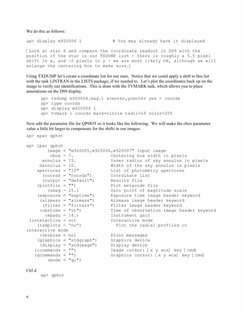
6

We do this as follows: ap> display m920006 1 # You may already have it displayed [Look at star 6 and compare the coordinate readout in DS9 with the position of the star in our TXDUMP list - there is roughly a 5.5 pixel shift in x, and ~2 pixels in y - we are most likely OK, although we will enlarge the centering box to make sure.] Using TXDUMP let’s create a coordinate list for our stars. Notice that we could apply a shift to this list with the task LINTRAN in the LISTS package, if we needed to. Let’s plot the coordinates back up on the image to verify our identifications. This is done with the TVMARK task, which allows you to place annotations on the DS9 display. ap> txdump m920004.mag.1 xcenter,ycenter yes > coords ap> type coords ap> display m920004 1 ap> tvmark 1 coords mark=circle radii=10 color=205 Now edit the parameter file for QPHOT so it looks like the following. We will make the cbox parameter value a little bit larger to compensate for the shifts in our images. ap> epar qphot ap> lpar qphot image = "m920005,m920006,m920007" Input image cbox = 7. Centering box width in pixels annulus = 15. Inner radius of sky annulus in pixels dannulus = 10. Width of the sky annulus in pixels apertures = "10" List of photometry apertures (coords = "coords") Coordinate list (output = "default") Results file (plotfile = "") Plot metacode file (zmag = 25.) Zero point of magnitude scale (exposure = "exptime") Exposure time image header keyword (airmass = "airmass") Airmass image header keyword (filter = "filters") Filter image header keyword (obstime = "ut") Time of observation image header keyword (epadu = 14.) Instrument gain (interactive = no) Interactive mode (radplots = “no”) Plot the radial profiles in interactive mode (verbose = no) Print messages (graphics = "stdgraph") Graphics device (display = "stdimage") Display device (icommands = "") Image cursor: [x y wcs] key [cmd] (gcommands = "") Graphics cursor: [x y wcs] key [cmd] (mode = "ql") Ctrl d ap> qphot

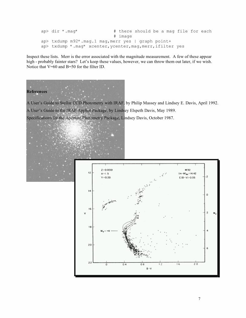
7

ap> dir *.mag* # there should be a mag file for each # image ap> txdump m92*.mag.1 mag,merr yes | graph point+ ap> txdump *.mag* xcenter,ycenter,mag,merr,ifilter yes Inspect these lists. Merr is the error associated with the magnitude measurement. A few of these appear high - probably fainter stars? Let’s keep these values, however, we can throw them out later, if we wish. Notice that V=60 and B=50 for the filter ID.

References A User’s Guide to Stellar CCD Photometry with IRAF, by Philip Massey and Lindsey E. Davis, April 1992.

A User’s Guide to the IRAF Apphot Package, by Lindsey Elspeth Davis, May 1989.

Specifications for the Aperture Photometry Package, Lindsey Davis, October 1987.

8

9

Name:___________________________________________________________ Date:_________________

IRAF Exercise 4 WorksheetIRAF Exercise 4 Worksheet

1. How can you tell, from the image header, whether CCDPROC has been run on a frame? 2. What’s one way to “patch” an image header, making sure it has information a task needs? 3. Does the way that QPHOT defines an aperture and sky region differ from what we saw when we used RIMEXAMINE in Exercise 2? Review both and explain briefly here. 4. How can you find out what quantities are listed in the m920004.mag.1 file? Specifically, which column in the file lists the magnitude error?

The qphot task can be used to determine aperture photometry values for a set of apertures, rather than a just one single one. Load the digiphot and apphot packages, then epar qphot so to set a list of multiple apertures:

image = "m920004" Input image cbox = 5. Centering box width in pixels annulus = 15 Inner radius of sky annulus in pixels dannulus = 10 Width of the sky annulus in pixels apertures = "1,2,3,4,5,10" List of photometry apertures (coords = "") Coordinate list (output = "default") Results file (plotfile = "") Plot metacode file (zmag = 25.) Zero point of magnitude scale (exposure = "exptime") Exposure time image header keyword (airmass = "airmass") Airmass image header keyword (filter = "filters") Filter image header keyword (obstime = "ut") Time of observation image header keyword (epadu = 14.) Instrument gain (interactive = yes) Interactive mode (radplots = yes) Plot radial profiles in interactive mode (verbose = no) Print messages (graphics = "stdgraph") Graphics device (display = "stdimage") Display device (icommands = "") Image cursor: [x y wcs] key [cmd] (gcommands = "") Graphics cursor: [x y wcs] key [cmd] (mode = "ql")

10

5. Now run qphot on m920004 again, but this time with multiple apertures. (It’s easiest to kill the graphics window each time before starting qphot). Concentrate on star #7, in the terminology of the finding chart. Place the cursor over the object and hit the space bar. Fill in Table I below, where Mag(i) refers to the magnitude obtained within a radius of i pixels. X Y Sky Mag(1) Mag(2) Mag(3) Mag(4) Mag(5) Mag(10)

Table I. Aperture Photometry data for Object 7 in m920004.fits 6. How much more flux (in ADU’s) fell within a 5 pixel radius, compared to the flux within a 2 pixel radius? Recall that Δmag= −2.5 log(F1/F2)! 7. Now repeat the multi-aperture qphot measurement, but for star #9, and fill in Table 2. All you need to do is place the cursor over the object and hit the space bar. X Y Sky Mag(1) Mag(2) Mag(3) Mag(4) Mag(5) Mag(10)

Table II. Aperture Photometry data for Object 9 in m920004.fits 8. By now you have (I hope!) realized that it requires a large aperture to actually integrate all the light from an object. In crowded regions, this is problematic, and also it folds in a lot of sky photons that add to the noise in the measurement. As long as the Point Spread Function (PSF) is constant across the image, you can make good relative measurements (i.e. differences in magnitudes between objects) with a small aperture. Use the results from tables I and II to complete table III, with Δmag=mag(object 7) – mag(object 9).

ΔMag(1) ΔMag(2) ΔMag(3) ΔMag(4) ΔMag(5) ΔMag(10)

Table III. Aperture Photometry comparison for Objects 7 and 9 in m920004.fits 9. Does the magnitude difference between objects 7 and 9 depend very strongly on the aperture chosen? How have you defined “very strongly”? What does this imply for differential photometry? 10. [For now, we are going to do this the long tedius way (unless you already know supermongo), and in a week or so (after we’ve all learned supermongo), we’ll do it the astrophysicists’ way: quick and easy!] Work with TXDUMP and just the m920004 and m920006 images. Extract the xcenter, ycenter, and magnitudes for the 9 stars, and put the information into a file. Making sure you’ve matched the data for each star between files, list the V magnitudes, B magnitudes, and B-V magnitudes (use Excel or another spreadsheet if you like). Plot V against B-V, making sure that the smallest V magnitude is at the top of the y-axis and the largest at the bottom. [This is actually quite easy to do in Excel by double clicking on the y-axis of the chart and checking under “scale”: values in reverse order, value (x) crosses at maximum value.] Although the magnitude offsets are wrong (we have no standard stars to guide us and an inaccurate sky magnitude), the two bluest stars are probably part of the horizontal branch, and the rest are on the red giant branch. Attach your plot to this worksheet.

5/5/05 IRAF5.doc 1

ASTRO 480ASTRO 480-- IRAF TUTORIAL : Introduction to DAOphotIRAF TUTORIAL : Introduction to DAOphot PSF fitting and DAOphot Some Advantages to PSF fitting The original motivation for psf fitting methods was for crowded field photometry, where often stellar images are blended and any reasonable-size aperture might include more than one star. DAOphot was developed by Peter Stetson at the Dominion Astrophysical Observatory, Victoria BC, for precise ground-based photometry in the crowded fields of globular clusters. It has since been incorporated into IRAF as the PSF fitting package there. If you want to know all the gory details see Stetson (1987). However, even for uncrowded environments, psf methods may still yield improved signal-to-noise of >10% compared to aperture photometry, since more of the available information is being used. The profiles of stars from the ground have been found to consist of an approximately Gaussian core, due to seeing (which may well vary), plus large wings decreasing only as an inverse square in intensity, largely a result of atmospheric scattering off dust and aerosols, plus dirt and scratches in the optical system. Use of profile-fitting techniques can remove most of the variations due to seeing changes, as well as enabling larger effective radii to be used. Procedure (in DAOphot) Here is a summary of the procedure one must follow: 1) Find all the stars on the frame above a user-set brightness threshold. The routine daofind in daophot convolves a Gaussian profile (of approximately the correct FWHM-psf) with each pixel, and can therefore discriminate between extended sources, stars, cosmic rays and CCD defects. 2) Run aperture photometry upon all the stars. 3) Deselect stars too close to the edge, or too faint and not within a group. Choose a set of bright, isolated stars spread across the frame – the “psf” stars. 4) Build a semi-empirical model psf. Each of the psf stars is scaled according to its aperture magnitude estimate, the weighted average is then fitted with a suitable analytic function, and a look-up table computed of the residuals (interpolating between the remainder value for each pixel). The analytic functions used are chosen from bivariate Gaussian, Moffat or Lorentz functions (or you can set the parameter to “auto” and it finds the best). An iterative procedure may be required to produce a `clean' psf in some cases, whereby psf modelling and fitting is performed, faint neighbors of psf stars are identified on a frame with the psf stars subtracted, fitted themselves and subtracted and the procedure repeated. 5) Using the centroid of a star as the profile center, and sky level as determined for aperture photometry, the PSF model is shifted and scaled to fit the observed stellar image by non-linear least-squares. The scaling yields the magnitude estimate. 6) To cope with the blending of stellar PSFs, the stars are grouped together before fitting if there is overlap, and each star in a group is fitted at the same time. Although the psf is modelled over a large radius (typically twice the FWHM), one may choose the central region over which the fitting is done: ~1x FWHMpsf works well; that is, we choose the same radius as was used for the preceding aperture photometry.

THINK:

Read over these 6 summaries and see if you can (mentally) translate them from “astrospeak” to “student-speak.” What does “FWHM” (full-width, half-max) refer to? Why might we expect ‘seeing’ to produce a Gaussian curve from the light produced by a point source?

2

Using DAOphot In this assignment you will be asked to log your data onto the worksheet attached at the end. Because the final results depend crucially on your answers at the beginning, make sure you check your parameters with your instructor. For clarity, here is a flowchart showing the various steps involved. Review these steps and consider whether they seem reasonable. We'll go through them (along with some intermediate steps) with the M92 dataset:

Generate coordinate list for all stars (daofind)

Perform aperture photometry (phot)

Select PSF template stars

(pstselect)

Generate model PSF (psf)

Perform PSF fitting photometry (allstar)

Figure 1. PSF fitting photometry flowchart

Throughout this handout, we will use “m920004” as the image you work on. However, this would just be a fully processed (i.e. bias- and dark-subtracted, and QE corrected image) image that you want to do photometry on – one with many, many stars in the field. Make sure you use only the processed M92 files. Generating the star coordinate list (you will do the next steps for both m920004 and m920006) First you need to set the characteristics of the CCD image data in the datapars file. daoedit is a useful task for this, providing you with information on the FWHM psf of stars, sky mean and sky sigma. cl> digiphot # load packages di> daophot # load package di> disp m920004 1 da> daoedit m920004 ? # list cursor options a # get stats such as FWHMpsf, sky mean and # sigma tabulated in command window. The cursor will jump automatically between windows! Repeat for a number of stars in this image, and determine representative values for these parameters. You may wish to calculate the means of the FWHMpsf, sky, and sigma to help you estimate the values to use. Now do Problem #1. We’re getting set up to determine parameter values for datapars. The values we set for these parameters are crucial to the success of DAOphot! After you determine your values, we’ll check them against those of your instructor to make sure that you aren’t too far off.

3

Now do Problem #2 – noting the values for additional critical parameters as follows: datamin #advise skymean – estimate roughly as (5 x sky sigma) datamax #with gain of 14, and assuming full well-depth #of 100,000 electrons, and at least 15 bit ADU's #estimate a reasonable value readnoise # 10 for this CCD epadu # 14 for these data exposure # for this and the remaining parameters, check the # image header for suitable keywords filter # keyword for filter obstime # keyword for time of observation After you have completed this section, compare your values to those on an instructor's copy of the datapars listing. COMPREHEND? What would happen with the number of stars selected if you set datamin too low? Too high? We will be working with images of a globular cluster taken through a visual and a blue filter. Would you expect the datamin (minimun detection threshold) would be greater or less in the visual filter than in the blue? For a given datamin, would you expect more stars to be selected in the visual image or the blue? Explain. Why would we want to even set a datamax value? What may happen within the program itself if we just set it at the saturation level? These questions will be important very shortly for you. Be sure you can answer them before going on. Ask your instructor if you are seeing these concepts through “cloudy skies.” Now, let’s set the program to work. da> daofind m920004 # the defaults should be okay; detection # threshold may require adjustment da> tvmark 1 m920004.coo.1 mar=cir rad=3 # mark ID'd stars on # image (THIS IS COOL!) da> txdump >> m920004.coo #generate ascii coordinate list m920004.coo.1 #answer prompt xc,yc #answer prompt xc>3 && xc<316 && yc>3 && yc<508 # optional exclusion of stars # too close to chip edges Note: I could not get this to work. da> tvmark 1 m920004.coo mar=cir rad=4 # check results In m920004.coo you now have a list of all stars upon which daophot thinks it can perform psf fitting.

4

Perform aperture photometry The routine phot uses a number of different parameter files: its very own photpars, the general CCD image one (datapars), one for centering (centerpars) and yet another for the sky fitting (fitskypars). You need to edit each of these. [Read through the list of parameters, leaving most of them at their default values, unless listed here. If you think a parameter is important, ask about it!] da> epar photpars apertures= ? # choose an appropriate aperture size # for “relatively faint” stars da> epar centerpars calgorithm = centroid cbox = 5.0 da> epar fitskypars salgorithm = mode annulus = # you choose sensible value! dannulus = # you choose sensible value! Now do Problem #3. After marking down your choices, compare them with those of a classmate and then your instructor before proceeding. da> lpar phot # what’s there? Do you see where it # “calls” the other tasks? da> phot m920004 m920004.coo # and use defaults, produces output # file m920004.mag.1 (same as qphot) You will find out (if you haven’t already) that if you ran qphot more than once, you got more than one “.mag” file for an image. The second file was named “.mag.2” – if you ran it again: “.mag.3” etc., because the program won’t overwrite a mag file if one already exists, it just automatically produces a new one with a different end number. Which mag file has the data you want? Meaning, which mag file is the one where the analysis went right? The one with the accurate data? When you see *.mag.1 referred to below, you may need to substitute a *.mag.2 or a *.mag.3 file instead. Keep track of what you are doing and where you are! [Sometimes easier said than done.] The same method of naming files happens with the .coo files as well, so BEWARE! Sel ect PSF template stars First you must set your psf parameters: da> epar daopars function = auto psfrad = # the radius within which the star’s # psf is defined; choose appropriate fitrad = # region in which fitting performed Then select your stars interactively: da> epar pstselect maxnpsf = 5 # 5 stars is a reasonable number of stars # to use to make a template. The fainter # they are, the more you need- all a interac = yes # matter of making a good model

5

Now run pstselect: da> pstselect m920004 ? # list the cursor commands. Select # suitable psf stars (i.e. bright and # isolated), saving each one as desired, # until you reach maxnpsf, save and quit) # breaks down to “a” in image, and “a” in # graph as you examine the 3-D profile. da> ls # directory should list m920004.pst.1 file Now, go back to the and do the steps once again for m920006. Think of whether or not you need to change some of the parameters when dealing with the blue image. Since we will be graphing the visual magnitude against the B-V color, what we want is the same stars to be in both lists. This may come at the expense of throwing some of the V stars out, or getting closer to the noise level in the B image. Right? Generate the model PSF da> ls m920004.fits m920006.fits >im.lis # generate list of images da> ls *.mag.1 >mag.lis # generate corresponding list of mag files # WATCH the ‘version’ numbers! da> ls *.pst.1 >pst.lis da> psf @im.lis @mag.lis @pst.lis interac- #run psf non-interactively Here, we ran the psf task two times, once for each filter. We could have done it a couple more times for the other two images (one more V, one more B), but you get the idea. What would we have done if we had 50 images instead! More time would have to be spent examining the images. What we want the program to do is maintain the same order of stars and IDs. If that happened, then we could list all of the images in a batch file, and let the computer go wild. In this case, there is too much of an x-y shift between the two images, and the number of stars selected uneven between filters to make this work well enough for us to try it. We are going to examine the model PSF (the “perfect” profile for stars in these images). Before you do so, see what seepsf does. What is input? What is output? Then, examine the model PSF. da> lpar seepsf da> seepsf m920004.fits.psf.1 m920004.fits.psf.1s da> seepsf m920006.fits.psf.1 m920006.fits.psf.1s da> disp m920004.fits.psf.1s # display in frame da> disp m920006.fits.psf.1s # display in frame da> imexam #use imexam to check that profile #looks like that of single star #NO EVIDENCE of contamination from #near neighbors for both images

Now do Problem #4.

6

Perform PSF fitting photometry

da> ls *psf.1.fits > psf.lis # generate list of psf files da> allstar @im.lis @mag.lis @psf.lis # finally psf fitting #photometry produces *.als.1 files Do something with your results: make a color-magnitude diagram 1. Extract the following information from both *.als.1 files: ID, XCENTER, YCENTER,MAG,MERR directing your output to two files. Find out how many stars had photometry done on them for each filter by giving the following Linux command (shown here as if you were still in IRAF) for each file: da>!wc –l yourfilename If there isn’t a huge difference in the number of stars (there will be 1 per line), then go with what you have. If there is a large difference, say 25% or so, then you can still continue with what you have, although the next step will be more tedious. 2. Load the data into a spreadsheet program 3. Calculate what the offset is between the V-image and the B-image. (I found this was easiest to do just using the images in ds9 and the cursor coordinates for a handful of stars.) 4. Within the spreadsheet, adjust the X & Y coordinates for one of the images so that they correspond to what they would be in the other image. (You are doing a “manual” shift.) 5. Match the stars in the two lists, getting rid of those stars that do not have a corresponding V or B component. 6. Calculate B-V and graph a color-magnitude diagram. This one will be turned in. We won’t need to have the tables of data, since your graph will say everything! References Stetson, Peter B , “DAOPHOT - A computer program for crowded-field stellar photometry”, 1987 PASP, 99, 191 A Reference Guide to the IRAF/DAOPHOT Package, Lindsey E. Davis, January 1994 \

7

Name:________________________________________________________________ Date:____________

IRAF EXERCISE 5 – Introduction to DAOPhot 1. Fill in the following table with the values for daoedit for the 10 stars listed.

V FILTER x y Sky Mean Sky sigma FWHMpsf Counts

B FILTER (you choose the stars)

x y Sky Mean Sky sigma FWHMpsf Counts

2. Edit datapars. What values did you choose for the following parameters?

V Filter B Filter fwhmpsf: fwhmpsf: sigma: sigma: datamin: datamin: datamax: datamax: readnoise: readnoise: epadu: epadu: 3. What values do you think are appropriate for: V Filter B Filter photpars.aperatures: fitskypars.annulus: fitskypars.dannulus: 4. What value for the FWHM did psf determine? V Filter _________ B Filter __________

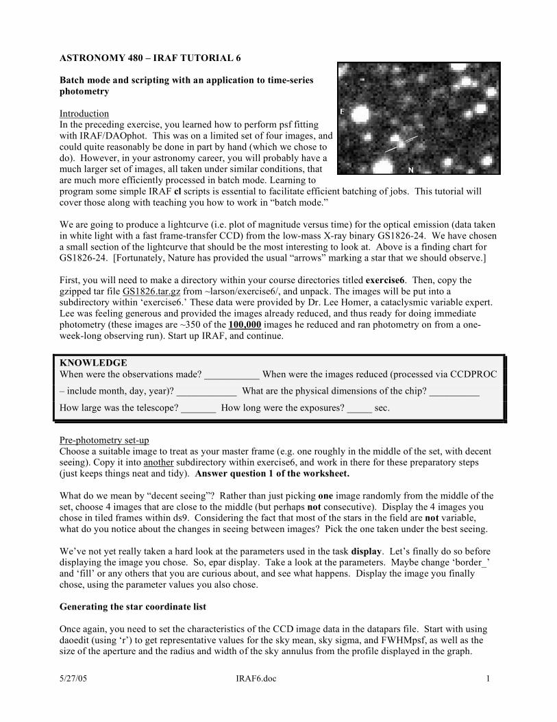
5/27/05 IRAF6.doc 1

ASTRONOMY 480 – IRAF TUTORIAL 6

Batch mode and scripting with an application to time-series photometry Introduction In the preceding exercise, you learned how to perform psf fitting with IRAF/DAOphot. This was on a limited set of four images, and could quite reasonably be done in part by hand (which we chose to do). However, in your astronomy career, you will probably have a much larger set of images, all taken under similar conditions, that are much more efficiently processed in batch mode. Learning to program some simple IRAF cl scripts is essential to facilitate efficient batching of jobs. This tutorial will cover those along with teaching you how to work in “batch mode.” We are going to produce a lightcurve (i.e. plot of magnitude versus time) for the optical emission (data taken in white light with a fast frame-transfer CCD) from the low-mass X-ray binary GS1826-24. We have chosen a small section of the lightcurve that should be the most interesting to look at. Above is a finding chart for GS1826-24. [Fortunately, Nature has provided the usual “arrows” marking a star that we should observe.] First, you will need to make a directory within your course directories titled exercise6. Then, copy the gzipped tar file GS1826.tar.gz from ~larson/exercise6/, and unpack. The images will be put into a subdirectory within ‘exercise6.’ These data were provided by Dr. Lee Homer, a cataclysmic variable expert. Lee was feeling generous and provided the images already reduced, and thus ready for doing immediate photometry (these images are ~350 of the 100,000 images he reduced and ran photometry on from a one-week-long observing run). Start up IRAF, and continue.

KNOWLEDGE When were the observations made? ___________ When were the images reduced (processed via CCDPROC

– include month, day, year)? ____________ What are the physical dimensions of the chip? __________

How large was the telescope? _______ How long were the exposures? _____ sec.

Pre-photometry set-up Choose a suitable image to treat as your master frame (e.g. one roughly in the middle of the set, with decent seeing). Copy it into another subdirectory within exercise6, and work in there for these preparatory steps (just keeps things neat and tidy). Answer question 1 of the worksheet. What do we mean by “decent seeing”? Rather than just picking one image randomly from the middle of the set, choose 4 images that are close to the middle (but perhaps not consecutive). Display the 4 images you chose in tiled frames within ds9. Considering the fact that most of the stars in the field are not variable, what do you notice about the changes in seeing between images? Pick the one taken under the best seeing. We’ve not yet really taken a hard look at the parameters used in the task display. Let’s finally do so before displaying the image you chose. So, epar display. Take a look at the parameters. Maybe change ‘border_’ and ‘fill’ or any others that you are curious about, and see what happens. Display the image you finally chose, using the parameter values you also chose. Generating the star coordinate list Once again, you need to set the characteristics of the CCD image data in the datapars file. Start with using daoedit (using ‘r’) to get representative values for the sky mean, sky sigma, and FWHMpsf, as well as the size of the aperture and the radius and width of the sky annulus from the profile displayed in the graph.

2

INSIGHT You are going to be changing parameters of DATAPARS. Do a phelp for datapars. How does the task use the value you set for fwhmpsf? What would happen if you set an enormously wrong value for the skysigma? How do the recommendations for datamin and datamax differ from what we did under IRAF5 – DAOphot? Take a look at question 2. Once you have the values for the sky, skysigma, and fwhmpsf, set them and the other critical parameters within datapars [epar datapars] datamax # with gain 2.5, full well-depth of 100,000 electrons, # and a 15 bit ADU estimate reasonable value [this # formula works here – what you WANT is not to go higher # than the linear part of the chip] – you can also use # INDEF readnoise # 10 for this CCD epadu # 2.5 for these data Now, answer Question 2 on the worksheet. [Don’t forget to review the other parameters and what datapars has for parameters to make sure all values or keywords are consistent with these images!] (You are still working in your special subdirectory.) Now create a star list with daofind, checking your results with tvmark. You may wish to do a phelp for daofind and tvmark, to make sure you understand what, exactly, it is they are doing and what they may be capable of doing beyond our use. You may find it helpful to actually epar tvmark to set the parameters. Check what daofind pulled out for stars. Did it “find” stars closely buried within the sky? Should you reset datamin? Datamax? Skysigma? FWHMpsf? This is where you gain experience making judgments and seeing the results. Make sure the parameters you set actually recover the target star. REVIEW You are going to run phot. Do an ‘lpar phot’ and list what other tasks it calls: You will need to make sure that ALL of the tasks that are called have the parameters set to appropriate values. How would you figure out what other tasks are called and which are just parameters?

5/27/05 IRAF6.doc 3

You may wish to ‘unlearn’ each task before epar’ing them. Now is a good time to review IRAF5. Start with where you did daoedit. What steps did you take after that? What parameters were changed? How will their values change for this exercise? Run phot. Check the results! Was the photometry successful or were there lots of errors? If there were lots of errors, what adjustments can/should you make? We actually need good photometry on just a few stars – the target star and a few comparison stars – but try to get good photometry on a half-dozen stars at this stage. Generating your psf star file (*.pst.1) With pstselect, select two or three bright, fairly isolated psf stars (there are only about that many suitable in this very small field). Remember to set the critical parameter file values for all the tasks that are called (note: this time we don't want any centroiding at any stage). Check your choices against ours, file linked from our home page. Rename your *.coo.? file to master.coo and the *.pst.1 file to master.pst.1, and copy both to the /exercise6/image/ directory. [Be sure to cd to that directory before going any further, otherwise, this becomes an extremely short, and incorrect exercise!] Running the photometry Double-check that all your parameter values are set as you wish. [Note: this time we will not centroid each time, since the tracking of the telescope was very good and the stars do not move significantly over this short interval. Use “none” where possible.] You’ve set the parameters in datapars, centerpars, fitskypars, photpars – all required under the task phot. Important: There is a possibility that different versions of IRAF have different orders for the parameters listed in the parameter files. When you see something like the following in an IRAF script psf (s1,'default',"master.pst.1",'default','default','default') the script is calling the task psf and giving the first 6 parameters the values given inside the parentheses. Within allphot.cl, you have the line phot (s1,"master.coo",'default') Do these values make sense for the first 3 parameters? If not, what’s wrong? What do you need to do? DO PROBLEMS 3 AND 4 before going to the next step. Allphot.cl needs an input list of all of the image files. This file is called “im.lis.” You need to generate this file. Do it, and then to run the script type: da> cl <allphot.cl ..and watch it do all the work!!

DON’T PANIC You may find that allphot.cl stops before it gets through the entire list of images. You may find that it stops more than once. What to do? Well, you have around 350 images, all within a few minutes of each other. Could you spare a couple by not doing photometry on them? How would you get allphot.cl to ignore these stars? Would you want allphot.cl to start from the beginning if you eliminated an image, or would you want it to start where it left off? Write down your decisions here:

4

Some points to note: For certain stages of this process (like the aperture photometry), you could simply have used IRAF's list input capability to get it to photometer all the images. However, as we ran across in IRAF5, when you come to tasks like psf and allstar, it becomes a real pain to make up some of the lists it needs. This script takes an image, and does everything for that image, generating requisite inputs/outputs as it goes along. Once, it finishes (it takes about 15 minutes for the ~350 images), you'll have the whole set of *.als.1 files. Browse through a few of these files to see what information is there. Also, the script is currently set to create *.sub.1.fits images which show visually how well the PSF fitting has worked.

UNDERSTAND Compare the results of a psf image to its original image by displaying both for one of the images in ds9 in “tile” format. What has happened?

Extracting, processing and displaying the data. Extraction In principle, you want to write a program that will extract the useful information from the *.als.1 files. The final goal here will be to create time-stamps for each data value, and then sort the data into lists for each star, comprising on each line ‘time, mag, merr’ (NOTE: The time quoted should be for the middle of the observation; however, since these are 2-second exposures, and we will be quoting each time as the number of seconds elapsed from the start of the time series, we won’t worry about confirming this here. ) In practice, we are going to use txdump to extract from each .als.1 file the “otime, id, xcenter, ycenter, mag, merr” for each image⊗ and put the information into individual files. Rather than run txdump over and over again, we’re going to practice writing a cl script. Allstar was set not to write a rejects file, and so you should find that each dump of magnitudes has all the stars in the same order, certainly the stars numbered the same, which should simplify matters. Eventually you will want a set of files called something like star01.dat, star02.dat, .... etc. We are going to accomplish this in two ways: 1) using the IRAF task MKSCRIPT, and 2) using a simple IRAF script written especially for this purpose. Answer question 5 before going on. 1) Using the IRAF task MKSCRIPT (see the next page): The instructions for making an IRAF script using MKSCRIPT are attached to this tutorial. You should also do a ‘phelp mkscript’ to get more information on how this works. You should also realize that making such scripts is not efficient if you are running a process only once (something we probably don’t need to tell you). However, once you have a script that works, you can use it time and time again – saving you LOTS of time in the future! In this step, we will leave the decision up to you as to how many stars you choose for extracting data. You really only need your target star and three standard stars – how about those stars you used to model the PSF? Answer question 6 before going on. ⊗ We also need id (how do we know which star is which); xcenter and ycenter can be used as a check to make SURE that the stars are all numbered identically among frames.

5/27/05 IRAF6.doc 5

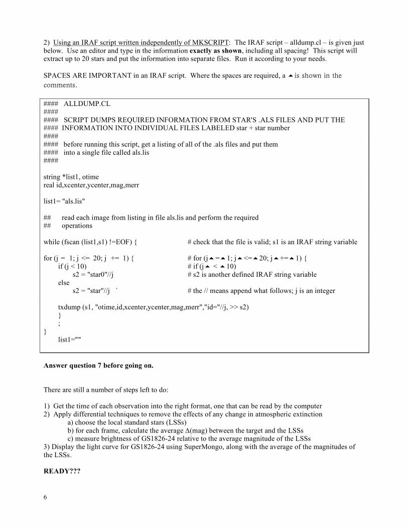
6

2) Using an IRAF script written independently of MKSCRIPT: The IRAF script – alldump.cl – is given just below. Use an editor and type in the information exactly as shown, including all spacing! This script will extract up to 20 stars and put the information into separate files. Run it according to your needs. SPACES ARE IMPORTANT in an IRAF script. Where the spaces are required, a is shown in the comments. #### ALLDUMP.CL #### #### SCRIPT DUMPS REQUIRED INFORMATION FROM STAR'S .ALS FILES AND PUT THE #### INFORMATION INTO INDIVIDUAL FILES LABELED star + star number #### #### before running this script, get a listing of all of the .als files and put them #### into a single file called als.lis #### string *list1, otime real id,xcenter,ycenter,mag,merr list1= "als.lis" ## read each image from listing in file als.lis and perform the required ## operations while (fscan (list1,s1) !=EOF) { # check that the file is valid; s1 is an IRAF string variable for (j = 1; j <= 20; j += 1) { # for (j=1; j<=20; j+=1) { if (j < 10) # if (j < 10) s2 = "star0"//j # s2 is another defined IRAF string variable else s2 = "star"//j ` # the // means append what follows; j is an integer txdump (s1, "otime,id,xcenter,ycenter,mag,merr","id="//j, >> s2) } ; } list1="" Answer question 7 before going on. There are still a number of steps left to do: 1) Get the time of each observation into the right format, one that can be read by the computer 2) Apply differential techniques to remove the effects of any change in atmospheric extinction a) choose the local standard stars (LSSs) b) for each frame, calculate the average ∆(mag) between the target and the LSSs c) measure brightness of GS1826-24 relative to the average magnitude of the LSSs 3) Display the light curve for GS1826-24 using SuperMongo, along with the average of the magnitudes of the LSSs. READY???

5/27/05 IRAF6.doc 7

Getting the time into the right format At this stage it is probably a good idea to change the UT times in hh:mm:ss into something more computer friendly; for the purposes of A480 and SM plotting, elapsed time in seconds from the start will be just fine.

UNDERSTANDING Assuming we have an computer program that will extract the hh mm ss from hh:mm:ss, what would your algorithm be for changing the UT to number of seconds from the start of the observations? Don’t peak at the computer program below! If we were going to plot every single star selected by ALLSTAR, we would want to replace any “INDEF” values with, for example, 99.0. Alternatively, you may wish to replace the INDEF with an interpolated magnitude and magnitude error value. We are going to use 3 stars as our standard stars (one of these should be of comparable magnitude to our target star). None of these should have any INDEF values for magnitudes. Check the files; make your decision. PERL script for manipulating columns in a file containing any number of columns – a computer language that is amazingly cryptic! Your file should have the .pl appended to its name. After you put this information into a file located in your images directory via vi or emacs (or textedit) and save it, you will need to do the following steps to run it successfully: 1) Make sure that you have extracted the data you need from the .als files. 2) Make this file executable by typing at the Linux command prompt chmod +x filename.pl In the way this is written, PERL needs to know what file has the data you want processed. Also, unless you want the information printed to the computer screen, you will need to tell PERL where you want the processed information to be put. Here is an example of what to type from the Linux command prompt: ]$ perl filename.pl file_with_star_data > name_of_output_file #!/usr/bin/perl –w # -w means ‘give warnings’ while (defined($line = <>)) # keep reading the lines until # EOF is reached (end of file) { chomp($line); # get rid of carriage return @list = split /\s+/, $line; # break line of data into individual columns # put data into an array @ut = split /:/, "$list[0]"; # split UT into usable numbers instead of # hh:mm:ss get hh mm ss in an array $t_hr = $ut[0] * 3600; # 1st element [0] has hour $t_min = $ut[1] * 60; # 2nd element [1] has min $t_sec = $ut[2]; # 3rd element [2] has seconds $t_obs = $t_hr + $t_min + $t_sec - 3920; # 3920 == UT at start print "$t_obs\t"; print "$list[4]\t"; # assumes col 5 has mag print "$list[5]\n"; # assumes col 6 has mag error }

8

Processing Next we want to apply differential techniques to remove the effects of any change in extinction; e.g., due to airmass changes (though for this short segment, that's insignificant), but certainly due to any passing clouds, or major seeing changes. Understanding In the next step, we are going to average the magnitudes for our LSS stars. Why would we prefer to use an average magnitude rather than the magnitude of just 1 star? Will this average magnitude be an average of the actual apparent magnitudes of the stars or an average of the instrumental magnitudes of the stars? Explain. We are using differential photometry. Here we subtract the average magnitude of the LSSs from the magnitude of the target star. Will this difference be an actual ∆(mag) or an average ∆(mag)? Explain. Choose, 1-3 bright stars (e.g. your PSF stars), which become your local standard stars (LSSs). Essentially one makes the assumption that these stars are constant (or at least do not vary over the time being analyzed). Therefore any change in their brightness will be due to systematic effects that will similarly affect your target star. What you are going to do is measure the brightness of GS1826-24 relative to the average magnitude of these bright stars. You will want to average the magnitude of the LSSs for each frame. Then, also for each frame, calculate the difference in magnitude ∆(mag) between the target and the LSSs average.

SUPERMONGO TO THE RESCUE! We could include this averaging of the LSSs magnitudes and calculations of average ∆(mag) between that average and the target star within our PERL script. However, SM will do it all for us, once we get the data read in from the various star data files produced by the PERL script. Write down the SM commands you would use to get the averages of the LSSs magnitudes and the ∆(mag): Displaying the lightcurve So finally, you should include in the work you turn in a plot having two panelsℵ: the top panel should show the differential lightcurve of the GS1826-24; the lower panel, on the same y scale and time interval, should show the plot of the average magnitude of the LSS stars. The reason for plotting the latter is to give you and the reader an empirical feel for the precision of your photometry, and indicate any times when the data deteriorated. ℵ Use the window command within SM.

5/27/05 IRAF6.doc 9

The lightcurve of GS1826-24 should be strikingly obvious: It shows an optical burst due to reprocessing in circumstellar material of an X-ray burst (an explosive runaway nuclear fusion event on the surface of the accreting neutron star). Be sure to get the magnitudes set up astronomically correct for the y-axes! References Stetson, Peter B , “DAOPHOT - A computer program for crowded-field stellar photometry”, 1987 PASP, 99, 191 A Reference Guide to the IRAF/DAOPHOT Package, Lindsey E. Davis, January 1994 http://iraf.noao.edu/iraf/docs/script.pdf :: An Introductory User’s Guide to IRAF Scripts

10

blank

5/27/05 IRAF6.doc 11

Name:_____________________________________ Date:_________

Astronomy 480 – IRAF Exercise VI -- Scripting 1. When we are observing a star with the goal of getting a long time series of data, optimally we would

choose to start early in the evening, on a date when the star transits at midnight, and end as late in the morning as possible. Considering this, when processing time series data, why is it important to pick a frame near the middle of the data set for choosing your PSF and comparison stars?

2. What values did you use for the following parameters in datapars?

fwhmpsf: datamax:

(sky) sigma: exposure (keyword):

datamin: obstime (keyword):

Check these with your instructor or with the parameter file linked from the course homepage (IRAF6_pars.pdf). The photometry for the stars in this image is slightly more sensitive to these values under DAOphot than was the photometry of the stars in M92. 3. In the space below, based upon the steps you did in IRAF5, draw a flowchart of how you think allphot.cl

should execute.

x y Sky Mean Sky sigma FWHMpsf

12

4. Now, decipher what allphot.cl actually does. To do this completely, you will need to find out what the task fscan and function access do. 5. Write down first how you think txdump would work if done the “long” way. What steps would you take? 6. Attach a copy of your cl script where you had IRAF do all of the work through the MKSCRIPT task. 7. Comment briefly on the result of using alldump.cl Must you use the data from all of the stars for which you have information, or would only the target star and a few standard stars do? (The way this is phrased, your answer should be obvious!) 8. Attach a copy of your sm macro, and light curves. Be sure your graph is complete – showing the data, having labeled axes, and identifying the stars for each of the curves. Include a suitable caption for the graph, one that tells the reader what you are displaying, giving enough information so that the graph stands on its own.

6/6/05 characterize_CCD.doc 1

Name __________________________________________

Astronomy 480 Characterizing a CCD [CCD Exercise I] Objectives In this exercise, you will characterize the following properties of the Kodak Enhanced KAF-0261E CCD that is part of the SBIG ST-9E or the Kodak KAF-1603E/ME that is part of the ST-8XEA camera:

• the detector gain and readnoise, • the detector linearity, • the detector dark current, and its dependence on temperature, and then • compare your results with the manufacturer specifications

Introduction The first charge coupled devices (CCDs) were produced just 30 years ago at Bell Labs in New Jersey. They have become the detector of choice for most astronomical observations in the UV and optical spectral regions, and are becoming increasingly popular for X-ray observations. There are a number of reasons for this popularity. The best CCDs have high quantum effciency (η ~ 90%), low readnoise (r ~ 2-3 e−), relatively uniform response, large dynamic range (D ≤ 100 dB) and excellent linearity. Virtually all large observatories maintain websites describing the characteristics of their CCDs, and it is important to know which detector is right for your observing program. It is also wise to measure and test these characteristics during the course of your observing run, rather than accept them as a matter of faith. I. Setting-Up the Camera and Computer Software See separate handout for instructions as the set up will depend on which camera you have and which computer you are using. Have your CD with manuals handy. Get your computer and camera ready to go. Play around a bit with the instrument and software to get familiar with them. You can set the number of automatic images that are taken, and how the images are numbered when saved. You can set the “title” of the image that will be placed in the image header. II. Detector Gain and Readnoise Every CCD relies on an amplifier to measure the electrons contained within the various detector pixels; readnoise is defined as the mean error contributed to a pixel by the amplifier. The amplifier signal is in turn digitized by an Analog-to-Digital (A-to-D) converter, and the gain is number of electrons per data unit produced in the conversion (i.e., e− per A-to-D conversion units, or ADUs). The lower the gain, the smaller the signal entering the A-to-D converter for a given number of electrons in the pixel (i.e., a low gain refers to a higher a value of e−/ADU).♣

♣ The signal coming from the amplifier is digitized by an analog-to-digital (A-to-D) converter and the gain is the number of electrons per data unit produced by the converter. This is inversely related to the gain of the amplifier (the terminology is a bit unfortunate). A lower gain for the amplifier means a smaller signal entering the A-to-D converter for a given number of electrons in the pixel and, thus, a large number of electrons per data unit. Conversely, a higher gain means fewer electrons per data unit.

2

It is possible to calculate the gain and readnoise by measuring the mean and standard deviations of pixel values in two pairs of images which have much different signal levels: i.e., a pair of bias images and a pair of flat-field images. In the bias images, the measured variation in the pixel values must arise solely from the readnoise of the amplifier for the simple reason that the image exposure time is zero seconds (i.e., the shutter never opens). The standard deviation of this variation is the readnoise. Given a bias image, it is a simple matter to calculate the readnoise in ADUs (Eqn. 1), but we are interested in its value in electrons. We will be taking 2 bias frames to form a difference image; you’ll find out why shortly.

!

"read

=Read Noise

Gain (1)

To convert from a readnoise measured in ADUs to one in electrons, we must also measure the amplifier gain. To measure the gain, we use exposures with much higher signal levels than the bias images, frequently dome or sky flat-field exposures. Once again, a pair of exposures is used to form a difference image, and the standard deviation is measured. In this case, though, the measured standard deviation contains a component from the pixel readnoise, and a random (Poisson) component due to the arrival time of the photons from the dome or sky. If the flatfield signal is strong enough, then the Poisson noise will be much greater than the read noise, and the standard deviation will be approximately:

!

"flat

=F #Gain

Gain (2)

The larger the gain, the larger the measured pixel-to-pixel deviation. We shall now follow Howell♦, p. 53. We will be taking 2 bias and 2 flatfield images. To find the gain:

!

Gain =F 1 + F 2( ) " B 1 + B 2( )# (F1"F2 )

2"# (B1"B2 )

2 , (3)

where the mean pixel values within each image are designated

!

F 1, F

2, and B

1, B

2, and the difference

images by

!

F1" F

2, and B

1" B

2.

Once we have the gain determined, we can calculate the read noise:

!

Read Noise =Gain"#

B1$B

2( )

2 (4)

Procedure for obtaining the images for read noise and gain calculations With the tube to the CCD totally covered, and the “save files” option on, take the bias frames. Getting decent flatfield images is going to be a challenge, since it is neither twilight nor are we in a dome. What we want is a diffuse source of light that will evenly expose the CCD and reveal any pixel-to-pixel variances. Try a white tissue, white cloth, or something similar.

♦ Howell, Steve B., Handbook of CCD Astronomy, 2000 (Cambridge University Press)

6/6/05 characterize_CCD.doc 3

Now, you may want to “uncheck” the save file box while we experiment with different exposure times. What we want from our flatfield is enough counts so that we are in the “shot noise” or Poisson noise regime, but not so many that we may introduce non-linearity concerns. Work with the exposure times until you get a maximum somewhere around 20,000 ADUs for the ST-9E and 15,000 for the ST-8XEA. Moving the cursor over the image will give you a reading. Once you’ve determined the exposure time, take a couple of flatfield images, making sure you save them to disk! III. Linearity of the CCD One the most appealing features of CCDs as astronomical detectors is their linearity, the degree to which the output signal is proportional to the incoming photons received by the detector. Examine the linearity of the CCD. Procedure for obtaining the images for the linearity determination Increase the exposure time of the flatfield until you get saturation. Then, expressing this exposure time as t, take a series of flatfield exposures of duration 1.00t, 0.80t, 0.60t, 0.40t, 0.20t, 0.10t, 0.05t, 0.025t, 0:0125t, 0:00625t, 0:003125t, and 0:0015625t. (There is, no doubt, a minimum exposure time for the camera – 0.12 sec.) Be sure to keep a record of your exposures. IV. Dark Current All CCDs contain a dark current caused by electrons which are boosted into the conduction band by thermal excitation. At room temperatures, this dark current will usually exceed most astrophysically interesting signals, but it can be suppressed by cooling the detector. The dark current should vary according to the empirical relation♦

!

DC = AT32 exp "

Eg

2kT

#

$ % &

' ( (5)

where A is a constant (must be something like ADUs per pixel per second per Kelvin3/2), Eg, is the the difference in energy between the Fermi level and the bottom of the conduction band for the semiconductor (the bandgap), and T is the detector temperature, in Kelvin. Temperature control for our CCDs is provided by a thermoelectric cooling system which produces a maximum reduction of around - 40 K below ambient. By measuring the dark current at different detector temperatures, clear up to room (ambient) temperature, it is possible to determine the values of A and Eg in equation (5). Procedure for obtaining the images for dependence on dark current with temperature With the CCD at its lowest temperature such that the load on the cooling system is not greater than 80% , take one dark frame of 20s, and save the frame. (A dark frame is an exposure in which the shutter does not open and the detector is not illuminated.) Record the CCD temperature. Now, turn off the cooling of the CCD until it reaches a temperature 5 degrees warmer than at the start. Let the CCD stabilize. Take a 20-sec exposure, making sure you save your data. Repeat until the CCD

♦ See also: http://www.kodak.com/global/plugins/acrobat/en/digital/ccd/applicationNotes/noiseSources.pdf

4

reaches room (ambient) temperature, probably 20 C. Once ambient temperature is reached, turn off the power, the camera and the computer controls, following the procedures in the user's manuals. V. Analysis [See IRAF steps on the last page when ready.] First, transfer the images from the data directory on your laptop or eMac to your course directory on an undergrad computer in B356. Close down the laptop or eMac properly. If there is time, go ahead and go to B356 and start your analysis even though the rest of the class and/or your instructor are still working getting images. Gain and Readnoise: Following the procedure described in II above, calculate the gain and readnoise of the CCD. Give the readnoise in both ADUs and electrons. In calculating the means and standard deviations, be sure to use the same region of the image (say, a subraster of 100 x 100 pixels) for both the biases and flat-fields. Try to avoid cosmetic defects such as bad columns, and regions which contain “hot" pixels or cosmic rays. Although the SBIG-9X CCD measures 512 x 512 pixels and the 8-XEA measures 1530 x 1020, be sure to avoid any ‘prescan’ or ‘overscan’ columns in your calculations. [Recall: The pixels in these regions do not really exist; they are generated by the readout electronics so that the zero level of the amplifier can be monitored.] Where are these regions? See the specifications for the CCD—there is just one column to the right of the image and one row at the top. You may wish to use either imstat in IRAF (where you will have to specify a subraster) or imexamine (that will take a subraster you specify in the parameters). For imstat, use the following format within IRAF (leave off the “.fits” and substitute the pixel ranges for the subraster in square brackets): cl> imstat filename[1:100, 1:100] Linearity: Using the series of exposures taken in III above, calculate the mean number of ADUs per pixel. Once again, try to avoid cosmetic defects, bad columns, cosmic rays, etc. Plot your mean counts in ADUs as a function of exposure time (see plotting instructions given on a separate sheet). Note that the actual exposure time may differ slightly from what you requested at the telescope; the actual time that the shutter was open is given in the image header under a keyword. Look for it. What is the best-fit linear relation? [See polyfit under IRAF.] What do you conclude about the linearity of the detector? Dark Current The dark current you are measuring is superimposed on a bias level which is non-zero. Use the overscan region of each CCD frame to calculate the net dark current in each exposure in ADUs per pixel per second (in other words, get rid of the bias level). Measure the mean pixel value, making sure not to include any bad columns or the overscan region. Before we determine the values of A and Eg which best fit the data, let’s take a closer look at the equation:

!

DC = AT32 exp "

Eg

2kT

#

$ % &

' ( .

What will DC converge to at high temperatures? What will determine the upper temperature limit? What will DC converge to at low temperatures? Plot the dark current as a function of temperature (see note that follows) and determine the value for the bandgap (and A, if possible). How does your derived value of Eg compare with the energy gap of

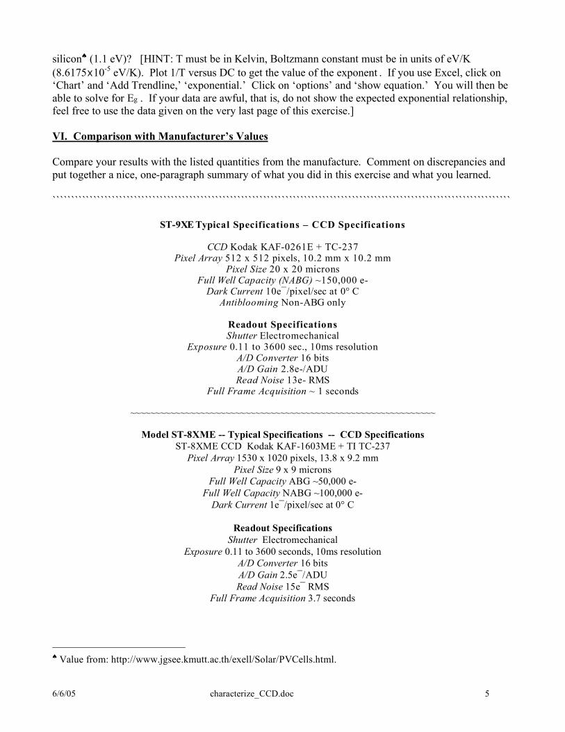
6/6/05 characterize_CCD.doc 5

silicon♠ (1.1 eV)? [HINT: T must be in Kelvin, Boltzmann constant must be in units of eV/K (8.6175x10-5 eV/K). Plot 1/T versus DC to get the value of the exponent . If you use Excel, click on ‘Chart’ and ‘Add Trendline,’ ‘exponential.’ Click on ‘options’ and ‘show equation.’ You will then be able to solve for Eg . If your data are awful, that is, do not show the expected exponential relationship, feel free to use the data given on the very last page of this exercise.] VI. Comparison with Manufacturer’s Values Compare your results with the listed quantities from the manufacture. Comment on discrepancies and put together a nice, one-paragraph summary of what you did in this exercise and what you learned. ````````````````````````````````````````````````````````````````````````````````````````````````````````````````````````````

ST-9XE Typical Specifications – CCD Specifications

CCD Kodak KAF-0261E + TC-237 Pixel Array 512 x 512 pixels, 10.2 mm x 10.2 mm

Pixel Size 20 x 20 microns Full Well Capacity (NABG) ~150,000 e-

Dark Current 10e¯/pixel/sec at 0° C Antiblooming Non-ABG only

Readout Specifications Shutter Electromechanical

Exposure 0.11 to 3600 sec., 10ms resolution A/D Converter 16 bits A/D Gain 2.8e-/ADU Read Noise 13e- RMS

Full Frame Acquisition ~ 1 seconds

~~~~~~~~~~~~~~~~~~~~~~~~~~~~~~~~~~~~~~~~~~~~~~~~~~~~~~~~~~~~~

Model ST-8XME -- Typical Specifications -- CCD Specifications ST-8XME CCD Kodak KAF-1603ME + TI TC-237

Pixel Array 1530 x 1020 pixels, 13.8 x 9.2 mm Pixel Size 9 x 9 microns

Full Well Capacity ABG ~50,000 e- Full Well Capacity NABG ~100,000 e-

Dark Current 1e¯/pixel/sec at 0° C

Readout Specifications Shutter Electromechanical

Exposure 0.11 to 3600 seconds, 10ms resolution A/D Converter 16 bits A/D Gain 2.5e¯/ADU Read Noise 15e¯ RMS

Full Frame Acquisition 3.7 seconds

♠ Value from: http://www.jgsee.kmutt.ac.th/exell/Solar/PVCells.html.

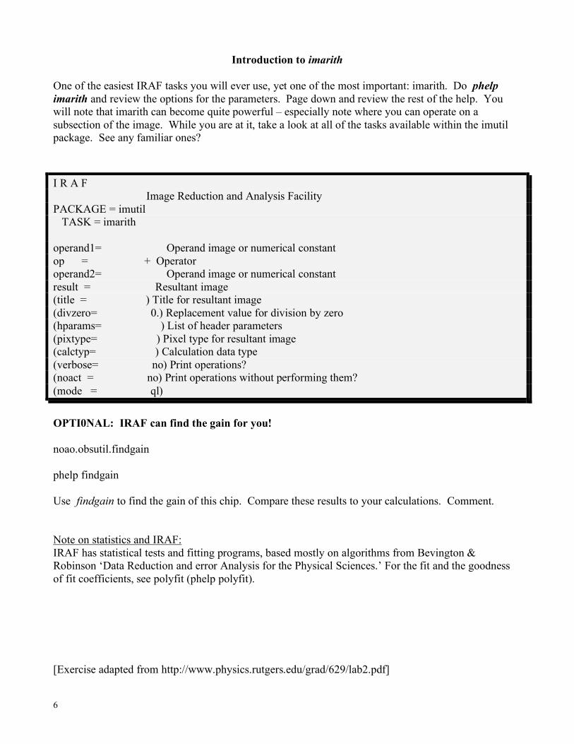
6

Introduction to imarith One of the easiest IRAF tasks you will ever use, yet one of the most important: imarith. Do phelp imarith and review the options for the parameters. Page down and review the rest of the help. You will note that imarith can become quite powerful – especially note where you can operate on a subsection of the image. While you are at it, take a look at all of the tasks available within the imutil package. See any familiar ones?

I R A F Image Reduction and Analysis Facility PACKAGE = imutil TASK = imarith operand1= Operand image or numerical constant op = + Operator operand2= Operand image or numerical constant result = Resultant image (title = ) Title for resultant image (divzero= 0.) Replacement value for division by zero (hparams= ) List of header parameters (pixtype= ) Pixel type for resultant image (calctyp= ) Calculation data type (verbose= no) Print operations? (noact = no) Print operations without performing them? (mode = ql)

OPTI0NAL: IRAF can find the gain for you! noao.obsutil.findgain phelp findgain Use findgain to find the gain of this chip. Compare these results to your calculations. Comment. Note on statistics and IRAF: IRAF has statistical tests and fitting programs, based mostly on algorithms from Bevington & Robinson ‘Data Reduction and error Analysis for the Physical Sciences.’ For the fit and the goodness of fit coefficients, see polyfit (phelp polyfit). [Exercise adapted from http://www.physics.rutgers.edu/grad/629/lab2.pdf]

6/6/05 characterize_CCD.doc 7

Using CCDSoft and MS Windows for This Exercise

One of the main goals for this exercise is to familiarize yourself with the software which controls the CCD that we use to take data from the sky. This program is called CCDSoft. It was written by the same company which built our ST-9E and ST-8XE CCDs, SBIG. Learning how to use your softare and hardware in the daylight is important! Only fools march up to a telescope in the middle of the night and think they can operate it! Before we begin with the software instructions, take a look at the CCD and the wires attached to it. See which wires are the power and which connects the camera to the computer. Look down the nozzle. You should see the chip itself. You should also create a subdirectory for your images. On the laptop, go to My Computer -> C:\ -> A480. Make a subdirectory there with your username. There is one absolutely mandatory thing you must remember about CCDSoft and the CCD itself. TURN OFF THE COOLING BEFORE YOU TURN OFF THE CCD!! Did you get that? Let's try again. TURN OFF THE COOLING BEFORE YOU TURN OFF THE CCD!! Okay. What do I mean by this? Remember that CCDs work best when cooled (we want those valence electrons to be cold, to minimize dark current). If you were to just turn off the CCD, you may send a power surge through the cooling electronics (it's just a thermocouple) which may fry the CCD chip. We consider this bad. Find the manual for CCD Soft onyour course CD! Have the pages on operating the SBIG camera at hand! With that said, let's talk about CCDSoft. CCDSoft is a windows based program which conforms to all the standard protocols of that OS. You will usually only need to deal with the “Camera” pulldown menu. CCDSoft has its own icon on the desktop. Once loaded, select “Camera -> Setup”. A new window should open (if it hasn't already) called “Camera Control”. Hit the Connect button to establish a link between the laptop and the CCD. Under Setup you can set the temperature of the chip. This is where you can also turn off the cooling! When setting the temperature you must try to balance keeping the chip as cool as possible, but not working the thermocouple too hard. In general you will want to keep the thermocouple at about 75%. So turn the cooling to on, and set the temperature (usually -10 to -15 is good). Watch the temperature display at the bottom of the Camera Control window. It will have some thermal momentum, but should, after about 5 minutes, settle down to a fairly constant value. From Camera Control you also take your images. There are many buttons and switches on this window, but we will, for the moment, only concern ourselves with the basics of taking an image. Select the “Take Image” tab (right next to the “Setup” tab). From this window we will set our exposure times, and decide how we want to deal with dark frames. Take the images as directed in the “procedure” part of this exercise, saving them as FITS files in your subdirectory. When finished, transfer these images to the USB memory stick. We will be transferring them over to one of the Apple computers, and then your account on one of the undergrad machines. [We've disconnected the Windows laptop from the internet. Why mess with viruses and updates when the Apples are so secure?] Shut Down Before you return to your computer to process the images, take a few minutes to explore CCDSoft. Open up the menus, and see what things are available. If you have any questions about these functions ask an instructor. Remember this is your one chance to prctice with the CCD before we use it for real. When you are done, TURN OFF THE COOLING. CHECK THE OPTIONS IN THE PROGRAM. DOES IT DO THIS AUTOMATICALLY FOR YOU?

Fig. 1 A picture of the ST-9E CCD. Light enters the nozzle on the left and lands on the chip located inside the housing. You attach the cables to the back and bottom.

8

BACK AT YOUR UNDERGRAD COMPUTER IN B356...... Notice that the images are saved with a .FIT extension. This annoyance is due to the fact that these images conform to Windows standards. However in our login.cl files we specify our images will be .fits. Therefore we must change these extensions. In ~larson/bin/ is a file called FIT2fits. This file changes the extension of every file in the directory from .FIT to .fits! This is just a Perlscript, so open it up and see if you understand how it works. Now that you have all of your files in your directory on your undergrad computer, continue with the Characterizing the CCD Exercise. We all know that biases and flatfields are quite boring, and here you’ve spent an afternoon working with NOISE, but so goes the early years of learning to be an astronomer. Besides, who knows when some interesting stuff will come out of the most mundane observations?

Using Equinox and Apple OS X for This Exercise

Equinox One of the main goals for this exercise is to familiarize yourself with the software which controls the CCD that we use to take data from the sky. This program, for the Apple iBook or eMac is called Equinox. It was not written by the same company which built our ST-9E and ST-8XE CCDs, SBIG, but rather a dedicated user who wanted the best in life. Learning how to use your softare and hardware in the daylight is important! Only fools march up to a telescope in the middle of the night and think they can operate it! Before we begin with the software instructions, take a look at the CCD and the wires attached to it. See which wires are the power and which connects the camera to the computer. Look down the nozzle. You should see the chip itself. You should also create a subdirectory for your images. On the laptop, go to Documents, Astro480, and make a subdirectory there with your username. There is one absolutely mandatory thing you must remember about the CCD itself. TURN OFF THE COOLING BEFORE YOU TURN OFF THE CCD!! Did you get that? Let's try again. TURN OFF THE COOLING BEFORE YOU TURN OFF THE CCD!! Okay. What do I mean by this? Remember that CCDs work best when cooled (we want those valence electrons to be cold, to minimize dark current). If you were to just turn off the CCD, you may send a power surge through the cooling electronics (it's just a thermocouple) which may fry the CCD chip. We consider this bad. Check the menus in Equinox. Is there a control switch that will prevent you from this horrendous end? Find the manual for Equinox onyour course CD! Have the pages on operating the SBIG camera at hand! Equinox is an OS X based program which conforms to all the standard protocols of that OS. You will usually only need to deal with the “Camera” pulldown menu. Equinox has its own icon on the desktop. Once loaded, select “Camera -> Setup”. A new window should open (if it hasn't already) called “Camera Control”. Hit the Connect button to establish a link between the laptop and the CCD. Under Setup you can set the temperature of the chip. This is where you can also turn off the cooling! When setting the temperature you must try to balance keeping the chip as cool as possible, but not working the thermocouple too hard. In general you will want to keep the thermocouple at about 75%. So turn the cooling to on, and set the temperature (usually -10 to -15 is good). Watch the temperature display at the bottom of the Camera Control window. It will have some thermal momentum, but should, after about 5 minutes, settle down to a fairly constant value.

Fig. 2 A picture of the ST-9E CCD. Light enters the nozzle on the left and lands on the chip located inside the housing. You attach the cables to the back and bottom.

6/6/05 characterize_CCD.doc 9

From Camera Control you also take your images. There are many buttons and switches on this window, but we will, for the moment, only concern ourselves with the basics of taking an image. Select the “Take Image” tab (right next to the “Setup” tab). From this window we will set our exposure times, and decide how we want to deal with dark frames. Take the images as directed in the “procedure” part of this exercise, saving them as FITS files in your subdirectory. When finished, transfer these images to the USB memory stick. We will be transferring them over to one of the Apple computers, and then your account on one of the undergrad machines. [We've disconnected the Windows laptop from the internet. Why mess with viruses and updates when the Apples are so secure?] Shut Down Before you return to your computer to process the images, take a few minutes to exploreEquinox. Open up the menus, and see what things are available. If you have any questions about these functions ask an instructor. Remember this is your one chance to prctice with the CCD before we use it for real. When you are done, TURN OFF THE COOLING. CHECK THE OPTIONS IN THE PROGRAM. DOES IT DO THIS AUTOMATICALLY FOR YOU? BACK AT YOUR UNDERGRAD COMPUTER IN B356...... Check to see what the extension is on the files that Equinox saves. Is it anything other than .fits? If it is, we will have to make an adjustment. Now that you have all of your files in your directory on your undergrad computer, continue with the Characterizing the CCD Exercise. We all know that biases and flatfields are quite boring, and here you’ve spent an afternoon working with NOISE, but so goes the early years of learning to be an astronomer. Some interesting stuff comes out of even the most mundane observations!

10

Data for Dark Current vs Temperature

(use if your data is awful)

Temperature (C)

Dark - Overscan (ADUs)

-10 60.12 -8 63.37 -7 91.56 -6 81.74 -5 86.0 -4 95.34 -3 105.7 -2 123.1 -1 133.7 0 140.5

Here is a more complete explanation of the relationship between dark current and temperature. The

value of the exponent is

!

"Eg

2kT .

http://www.kodak.com/global/plugins/acrobat/en/digital/ccd/applicationNotes/noiseSources.pdf