Astrophysical Black Holes: A Compact Pedagogical Review

Cosimo Bambi∗

Center for Field Theory and Particle Physics and Department of Physics, Fudan University, 200433 Shanghai, China andTheoretical Astrophysics, Eberhard-Karls Universitat Tubingen, 72076 Tubingen, Germany

(Dated: February 2, 2018)

Black holes are among the most extreme objects that can be found in the Universe and an ideallaboratory for testing fundamental physics. This article will briefly review the basic properties ofblack holes as expected from general relativity, the main astronomical observations, and the leadingastrophysical techniques to probe the strong gravity region of these objects. It is mainly intended toprovide a compact introductory overview on astrophysical black holes to new students entering thisresearch field, as well as to senior researchers working in general relativity and alternative theoriesof gravity and wishing to quickly learn the state of the art of astronomical observations of blackholes.

I. INTRODUCTION

A black hole is, roughly speaking, a region of the space-time in which gravity is so strong that nothing, nor evenlight, can escape. The event horizon is the boundary ofsuch a region. For a more rigorous definition, see e.g. [1]and references therein, but it will not be necessary forwhat follows.

The possibility of the existence of extremely compactobjects such that their strong gravitational field couldprevent the escape of light was first discussed by JohnMichell and Pierre-Simon Laplace at the end of the 18thcentury in the context of Newtonian mechanics. In thecorpuscular theory of light developed in the 17th century,light was made of small particles traveling with a finitevelocity c. Michell and Laplace noted that the escapevelocity from the surface of a body of mass M and radiusR exceeds c if R < Rcrit, where

Rcrit =2GNM

c2(1)

and GN is Newton’s gravitational constant. Such a com-pact body would not be able to emit radiation from itssurface and should thus look black.

The theory of general relativity was proposed by Al-bert Einstein at the end of 1915 [2]. The simplest blackhole solution was found immediately after, in 1916, byKarl Schwarzschild [3]. It described a non-rotating blackhole. However, its actual physical properties were onlyunderstood much later. David Finkelstein was the first,in 1958, to figure out that this solution had an eventhorizon causally separating the interior from the exteriorregion [4]. The solution for a rotating black hole in gen-eral relativity was found only in 1963, by Roy Kerr [5].

Even the astrophysical implications of such solutionswere initially not taken very seriously. Most people weremore inclined to believe that “some unknown mecha-nism” could prevent the complete collapse of a mas-sive body and the formation of a black hole in the Uni-

∗ E-mail: bambi@fudan.edu.cn

verse. In 1964, Yakov Zeldovich and, independently, Ed-win Salpeter proposed that quasars were powered by acentral supermassive black hole [6, 7]. In the early 1970s,Thomas Bolton and, independently, Louise Webster andPaul Murdin identified the X-ray source Cygnus X-1 asthe first stellar-mass black hole candidate [8, 9]. Sincethen, an increasing number of astronomical observationshave pointed out the existence of stellar-mass black holesin some X-ray binaries [10] and of supermassive blackholes at the center of many galaxies [11]. Thanks totechnological progresses and new observational facilities,in the past 10-20 years there have been substantial pro-gresses in the study of astrophysical black holes. InSeptember 2015, the LIGO experiment detected, for thefirst time, the gravitational waves emitted from the co-alescence of two black holes [12], opening a completelynew window for studying these objects.

It is curious that the term black hole is relatively re-cent. While it is not clear who used the term first, itappeared for the first time in a publication in the Jan-uary 18, 1964 issue of Science News Letter. It was on areport on a meeting of the American Association for theAdvancement of Science by journalist Ann Ewing. Theterm became quickly very popular after it was used byJohn Wheeler at a lecture in New York in 1967.

Black holes can potentially have any value of the mass,and the latter is the characteristic quantity setting thesize of the system. The gravitational radius of an objectof mass M is defined as

rg =GNM

c2= 14.77

(M

10 M�

)km . (2)

The associated characteristic time scale is

τ =rg

c= 49.23

(M

10 M�

)µs . (3)

It can be quite useful to have these two scales in mind.For M ∼ 106 M�, we find rg ∼ 106 km and τ ∼ 5 s. ForM ∼ 109 M�, we have rg ∼ 109 km and τ ∼ 1 hr.

When we discuss observations of astrophysical blackholes, an important concept is that of Eddington lumi-nosity. It is the maximum luminosity for a generic object,not necessarily a black hole. The Eddington luminosity

arX

iv:1

711.

1025

6v3

[gr

-qc]

31

Jan

2018

2

LEdd is reached when the pressure of the radiation lumi-nosity on the emitting material balances the gravitationalforce towards the object. If a normal star has a luminos-ity L > LEdd, the pressure of the radiation luminositydrives an outflow. If the luminosity of the accretion flowof a black hole exceeds LEdd, the pressure of the radiationluminosity stops the accretion process, reducing the lumi-nosity. Assuming that the emitting medium is a ionizedgas of protons and electrons, the Eddington luminosityof an object of mass M is

LEdd =4πGNMmpc

σTh

= 1.26 · 1038

(M

M�

)erg/s , (4)

where mp is the proton mass and σTh is the electronThomson cross section. For an accreting black hole, wecan define the Eddington mass accretion rate MEdd fromLEdd = ηrMEddc

2, where ηr ∼ 0.1 is the radiative effi-ciency of the accretion process, namely the fraction ofenergy of the accreting material emitted in the form ofelectromagnetic radiation.

II. BLACK HOLES IN GENERAL RELATIVITY

In 4-dimensional general relativity, black holes are rel-atively simple objects, in the sense they are completelycharacterized by a small number of parameters. This isthe result of the no-hair theorem, which holds under spe-cific assumptions [13–16]. The name no-hair is to indi-cate that black holes have only a small number of features(hairs). We have also a uniqueness theorem, according towhich black holes are only characterized by a family ofsolutions. Violations of these theorems are possible if werelax some of these assumptions or we consider theoriesbeyond general relativity.

A Schwarzschild black hole is a non-rotating and elec-trically uncharged black hole and is completely charac-terized by one parameter, the black hole mass M . AReissner-Nordstrom black hole is a non-rotating blackhole of mass M and electric charge Q. A Kerr blackhole is an uncharged black hole of mass M and spin an-gular momentum J . The general case is represented bya Kerr-Newman black hole, which has a mass M , a spinangular momentum J , and an electric charge Q.

In what follows, we will only consider Kerr black holes(which include the Schwarzschild case for vanishing spinangular momentum), because for astrophysical macro-scopic objects the possible non-vanishing electric chargeis extremely small and can be ignored [1]. Instead of Mand J , it is often convenient to use M and a∗, where a∗is the dimensionless spin parameter

a∗ =cJ

GNM2. (5)

Note that in Newtonian gravity the spin does not playany role; in Newton’s Universal Law of Gravitation we

0

2

4

6

8

10

0 0.2 0.4 0.6 0.8 1

r/rg

a*

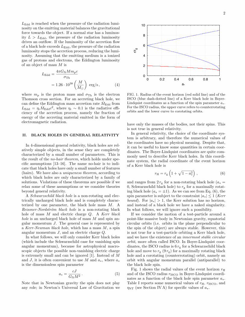
FIG. 1. Radius of the event horizon (red solid line) and of theISCO (blue dash-dotted line) of a Kerr black hole in Boyer-Lindquist coordinates as a function of the spin parameter a∗.For the ISCO radius, the upper curve refers to counterrotatingorbits and the lower curve to corotating orbits.

have only the masses of the bodies, not their spins. Thisis not true in general relativity.

In general relativity, the choice of the coordinate sys-tem is arbitrary, and therefore the numerical values ofthe coordinates have no physical meaning. Despite that,it can be useful to know some quantities in certain coor-dinates. The Boyer-Lindquist coordinates are quite com-monly used to describe Kerr black holes. In this coordi-nate system, the radial coordinate of the event horizonof a Kerr black hole is

rH = rg

(1 +

√1− a2

∗

), (6)

and ranges from 2 rg for a non-rotating black hole (a∗ =0, Schwarzschild black hole) to rg for a maximally rotat-ing black hole (a∗ = ±1). As we can see from Eq. (6), thespin parameter is subject to the constraint |a∗| ≤ 1 (Kerrbound). For |a∗| > 1, the Kerr solution has no horizon,and instead of a black hole we have a naked singularity.In what follows, we will ignore such a possibility.

If we consider the motion of a test-particle around apoint-like massive body in Newtonian gravity, equatorialcircular orbits (i.e. orbits in the plane perpendicular tothe spin of the object) are always stable. However, thisis not true for a test-particle orbiting a Kerr black hole,and we have the existence of an innermost stable circularorbit, more often called ISCO. In Boyer-Lindquist coor-dinates, the ISCO radius is 6 rg for a Schwarzschild blackhole and move to rg (9 rg) for a maximally rotating blackhole and a corotating (counterrotating) orbit, namely anorbit with angular momentum parallel (antiparallel) tothe black hole spin.

Fig. 1 shows the radial values of the event horizon rH

and of the ISCO radius rISCO in Boyer-Lindquist coordi-nates as a function of the black hole spin parameter a∗.Table I reports some numerical values of rH, rISCO, andηNT (see Section IV A) for specific values of a∗.

3

a∗ rH/rg rISCO/rg ηNT

-1 1 9 0.038

0 2 6 0.057

0.5 1.866 4.423 0.082

0.8 1.6 3.065 0.121

0.9 1.436 2.424 0.155

0.95 1.312 2.000 0.190

0.99 1.141 1.474 0.264

0.998 1.063 1.243 0.321

1 1 1 0.423

TABLE I. Properties of Kerr black holes. For every spinparameters a∗, the table shows the corresponding radius ofthe event horizon rH, the radius of the ISCO rISCO, and theradiative efficiency of a Novikov-Thorne disk ηNT [see Sec-tion IV A, where ηNT is defined in Eq. (8)]. rH and rISCO

in Boyer-Lindquist coordinates. a∗ > 0 (< 0) for corotating(counterrotating) orbits.

More details on black holes in general relativity can befound in [1, 17, 18].

III. ASTROPHYSICAL BLACK HOLES

From general relativity, there are no constraints on thevalue of the mass of a black hole, which can thus be arbi-trarily small as well as arbitrarily large. From astronom-ical observations, we have strong evidence of at least twoclasses of astrophysical black holes:

1. Stellar-mass black holes [10].

2. Supermassive black holes [11].

There is also some evidence of intermediate-mass blackholes, with a mass filling the gap between the stellar-mass and the supermassive ones [19]. Black holes shouldform from the complete gravitational collapse of a sys-tem, when there is no mechanics capable of balancingthe gravitational force and the system shrinks until theformation of the event horizon. The collapse of the coreof heavy stars is expected to produce black holes witha mass M >∼ 3 M� because for cores of lower mass thequantum pressure of neutrons should stop the collapseand the final product should be a neutron star [20–22].However, there are cosmological scenarios in which it ispossible to produce primordial black holes with any mass,even much lower than 3 M� [24]. Nevertheless, for themoment there is no evidence for the existence of suchobjects.

Note the different terminology employed in differentscientific communities. Among astronomers, it is com-mon to call “black hole” an astrophysical object that issupposed to be a black hole and for which there is adynamical measurement of its mass. The latter indeedguarantees that the object is (if it is compact) too heavy

for being a neutron star. “Black hole candidates” are in-stead astrophysical objects that are supposed to be blackholes but for which there is no dynamical measurementof their mass. In the theoretical physics community, ev-ery astrophysical object that is supposed to be a blackhole is called “black hole candidate” because it is onlypossible to put some constraints on the existence of theevent horizon, but it is impossible to get a proof.

A. Stellar-Mass Black Holes

From stellar evolution simulations, we expect that inour Galaxy there is a population of about 108−109 blackholes formed at the end of the evolution of heavystars [25, 26], and the same number can be expected insimilar galaxies. The initial mass of a stellar-mass blackhole should depend on the properties of the progenitorstar: on its mass, its evolution, and the supernova explo-sion mechanism [27]. A crucial quantity is the metallicityof the star, namely the fraction of mass of the star madeof elements heavier than helium.

The maximum mass of black hole remnants criticallydepends on the metallicity. The final mass of the rem-nant is indeed determined by the mass loss rate by stel-lar winds, which increases with the metallicity becauseheavier elements have a larger cross section than lighterones, and therefore they evaporate faster. For a low-metallicity star [28–30], there may be a mass gap in theremnant, roughly between 50 and 150 M�, namely themass of the black hole remnant can be M <∼ 50 M� orM >∼ 150 M�. As the metallicity increases, black holeswith M >∼ 150 M� disappear, mainly because of the in-creased mass loss rate. Note, however, that some modelsdo not find remnants with a mass above the gap, becausestars with M >∼ 150 M� may undergo a runaway ther-monuclear explosion that completely destroys the system,without leaving any black hole remnant [28, 29].

The lower bound may come from the maximum massfor a neutron star: the exact value is currently unknown,because it depends on the equation of state of matter atsuper-nuclear densities, but it should be around 2−3 M�.For bodies with a mass lower than this limit, the quantumneutron pressure can stop the collapse and the final prod-uct is a neutron stars. For bodies exceeding this limit, thefinal product is a black hole [20–22]. Note, however, thatthere may be a mass gap between the maximum neutronstar mass and the minimum black hole mass [23].

Stellar-mass black holes may thus have a mass in therange 3 − 100 M�. At the moment, all the knownstellar-mass black holes in X-ray binaries have a massM ≈ 3 − 20 M� [31]. Gravitational waves have shownthe existence of heavier stellar-mass black holes. In par-ticular, the event called GW150914 was associated to thecoalescence of two black holes with a mass M ≈ 30 M�that merged to form a black hole with M ≈ 60 M� [12].

While we expect a huge number of stellar-mass blackholes in the Galaxy, we only know about 20 objects with a

4

dynamical measurement of the mass and about 50 objectswithout a dynamical measurement of their mass (it isthus possible that some of them are not black holes butneutron stars). This is because their detection is verychallenging. The simplest case is when the black holeis in a binary system and has a companion star. Thepresence of a compact object can be discovered from theobservation of X-ray radiation emitted from the innerpart of the accretion disk (see Section IV for more detailsabout accretion). If we can study the orbital motion ofthe companion star, we may be able to measure the massfunction [31]

f(M) =K3

cPorb

2πGN=M sin3 i

(1 + q)2 , (7)

where Kc = vc sin i, vc is the velocity of the companionstar, i is the angle between the normal of the orbitalplane and our line of sight, Porb is the orbital period ofthe system, q = Mc/M , Mc is the mass of the companion,and M is the mass of the dark object. If we can somehowestimate i and Mc, we can infer M , and in this case wetalk about dynamical measurement of the mass. Thedark object is a black hole if M > 3 M� [20–22].

Black holes in X-ray binaries (black hole binaries1)are grouped into two classes: low-mass X-ray binaries(LMXBs) and high-mass X-ray binaries (HMXBs). Lowand high is referred to the stellar companion, not to theblack hole: in the case of LMXBs, the companion starhas normally a mass M < 3 M�, while for HMXBs thecompanion star has M > 10 M�. Observationally, wecan classify black hole binaries either as transient X-raysources or persistent X-ray sources. LMXBs are usuallytransient sources, because the mass transfer is not con-tinuos (for instance, at some point the surface of thecompanion star may expand and the black hole stripssome gas): the system may be bright for a period rang-ing from some days to a few months and then be in aquiescent state for months or even decades. We expect103 − 104 LMXBs in the Galaxy [32, 33] and every yearwe discover 1-2 new objects, when they pass from theirquiescent state to an outburst (see Section V A for moredetails). HMXBs are persistent sources: the mass trans-fer from the companion star to the black hole is a rel-atively regular process (typically it is due to the stellarwind of the companion) and the binary is a bright sourceat any time without quiescent periods.

Fig. 2 shows 22 X-ray binaries with a stellar-mass blackhole confirmed by dynamical measurements. To have anidea of the size of these systems, the figure also shows the

1 Generally speaking, a black hole binary is a binary system inwhich at least one of the two bodies is a black hole, and a binaryblack hole is a binary system of two black holes. In the contextof stellar-mass black holes, the term black hole binary is used toindicate a binary system of a black hole with a stellar companion.In the context of supermassive black holes, it is common to callblack hole binary a system of two supermassive black holes.

FIG. 2. Sketch of 22 X-ray binaries with a stellar-mass blackhole confirmed by dynamical measurements. For every sys-tem, the black hole accretion disk is on the left and the com-panion star is on the right. The color of the companionstar roughly indicates its surface temperature (from brownto white as the temperature increases). The orientation ofthe disks indicates the inclination angles of the binaries. Forcomparison, in the top left corner of the figure we see thesystem Sun-Mercury: the distance between the two bodiesis about 50 millions km and the radius of the Sun is about0.7 millions km. Figure courtesy of Jerome Orosz.

Sun (whose radius is 0.7 millions km) and the distanceSun-Mercury (about 50 millions km). The black holeshave a radius < 100 km and cannot be seen, but we canclearly see their accretion disks formed from the transferof material from the companion star. The latter mayhave a quite deformed shape (in particular, we can seesome cusps) due to the the tidal force produced by thegravitational field of the black hole. In Fig. 2, Cygnus X-1 (Cyg X-1 in Fig. 2), LMC X-1, LMC X-3, and M33 X-7are HMXBs, while all other systems are LMXBs. Amongthese HMXBs, only Cygnus X-1 is in our Galaxy. Amongthe LMXBs, there is GRS 1915+105, which is quite apeculiar source: since 1992, it is a bright X-ray sourcein the sky, so it can be considered a persistent sourceeven if it is a LMXB. This is probably because of itslarge accretion disk, which can provide enough materialat any time.

Black holes in compact binary systems (black hole-black hole or black hole-neutron star) can be detectedwith gravitational waves when the signal is sufficiently

5

strong, which means just before the merger (see Sec-tion VI E for more details). Fig. 3 shows the first de-tections by the LIGO/Virgo collaboration. The name ofthe event is classified as GW (gravitational wave event)and then there is the date: for example, GW150914 wasdetected on 14 September 2015. LVT151012 is not clas-sified as a gravitational wave event because it may havebeen caused by noise. For every event, the figure showsthe two original black holes as well as the final one aftermerger.

Isolated black holes are much more elusive. In princi-ple, they can be detected by observing the modulationof the light of background stars due to the gravitationallensing caused by the passage of a black hole along theline of sign of the observer [34].

B. Supermassive Black Holes

Astronomical observations show that at the center of alarge number of galaxies there is a large amount of massin a relatively small volume. The standard interpreta-tion is that these objects are supermassive black holeswith M ∼ 105 − 1010 M�. The strongest constraintscome from the center of our Galaxy2 and of NGC 4258by studying the motion of individual stars or of gas intheir nuclei. In the end, we can exclude the existence of acluster of compact non-luminous bodies like neutron starsand therefore we can conclude that these objects are su-permassive black holes [37]. In the case of other galaxies,

FIG. 3. Masses of the first black holes observed withgravitational waves, with the two initial objects merginginto a larger one, as shown by the arrows. Image Credit:LIGO/NSF/Caltech/SSU Aurore Simmonet.

2 The total mass of our Galaxy is estimated to be MMW ∼1012 M� [35]. The mass of the central supermassive black holeis M ≈ 4 · 106 M� [36].

it is not possible to put such constraints with the avail-able data, but it is thought that every middle-size (likeour Galaxy) or large galaxy has a supermassive black holeat its center3. For lighter galaxies, the situation is moreuncertain. Most models predict supermassive black holesat the center of lighter galaxies as well [39], but there arealso models predicting the existence of a population offaint low-mass galaxies with no supermassive black holeat their center [40, 41]. Observations suggest that somesmall galaxies have a supermassive black hole and othersmall galaxies do not [42, 43].

In the case of stellar-mass black holes, it is easy toargue that they are the final product of the evolutionof very heavy stars. In the case of supermassive blackholes, at the moment we do not know their exact origin.We observe supermassive objects in galactic nuclei witha mass M ∼ 105 − 1010 M�. More puzzlingly, we ob-serve objects with masses M ∼ 1010 M� even in verydistant galaxies [44], when the Universe was only 1 bil-lion years old, and we do not know how such objectswere created and were able to grow so fast in a relativelyshort time [39]. The Eddington accretion rate can be ex-ceeded in some accretion models, and this may indeed bea possible path to the rapid growth of supermassive blackholes [45]. The possibility of super-Eddington accretionis confirmed, for instance, by the observation of a neutronstar in the galaxy M82 with a luminosity exceeding itsEddington limit [46]. It is also possible that supermassiveblack holes formed from the collapse of heavy primordialclouds rather than of stars, or that they formed from themerger of several black holes [39].

C. Intermediate-Mass Black Holes

Intermediate-mass black holes are, by definition, blackholes with a mass between the stellar-mass and the su-permassive ones, say M ∼ 102−104 M�. At the moment,there is no dynamical measurement of the mass of theseobjects, and their actual nature is still controversial.

Some intermediate-mass black hole candidates are as-sociated to ultra luminous X-ray sources [47]. Theseobjects have an X-ray luminosity LX > 1039 erg/s,which exceeds the Eddington luminosity of a stellar-massobject, and they may thus have a mass in the range102−104 M�. However, we cannot exclude they are actu-ally stellar-mass black holes (or neutron stars [46]) withnon-isotropic emission and a moderate super-Eddingtonmass accretion rate [48].

The existence of intermediate-mass black holes is alsosuggested by the detection of some quasi-periodic oscil-lations (QPOs, see Section VI C) in some ultra-luminousX-ray sources. QPOs are currently not well understood,

3 Exceptions may be possible: the galaxy A2261-BCG has a verylarge mass but it might not have any supermassive black hole atits center [38].

6

but they are thought to be associated to the fundamentalfrequencies of the oscillation of a particle around a blackhole. Since the size of the system scales as the blackhole mass, QPOs should scale as 1/M , and some obser-vations may indicate the existence of compact objectswith masses in the range 102 − 104 M� [49].

Intermediate-mass black holes may be expected toform at the center of dense stellar clusters by merger.Several studies have tried to explore the possible exis-tence of these objects from the observations of the mo-tion of the stars in certain clusters. The presence of anintermediate-mass black hole at the center of the clus-ter should increase the velocity dispersion in the cluster.Some studies suggest that there are indeed intermediate-mass black holes at the center of certain globular clus-ter [50, 51], but there is not yet a common consensus.

IV. ACCRETION DISKS

A black hole itself cannot emit any radiation by def-inition. On the contrary, we can observe the radiationemitted by the gas in a possible accretion disk surround-ing the black hole. In the case of stellar-mass black holeswith a companion star, the disk is created by the masstransfer from the stellar companion to the black hole.In the case of supermassive black holes in galactic nu-clei, the disk forms from the material in the interstellarmedium [52] or as a result of galaxy merger [53, 54].

The accretion disk can have different shapes and dif-ferent properties, depending on its exact origin. Anaccretion disk is geometrically thin (thick) if h/r � 1(h/r ∼ 1), where h is the semi-thickness of the disk atthe radial coordinate r. The disk is optically thin (thick)if h� λ (h� λ), where λ is the photon mean free pathin the medium of the disk. If the disk is optically thick,we see the radiation emitted from the surface of the disk,like in the case of stars.

An important class of accretion disks is represented bythe geometrically thin and optically thick disks, which arecommonly described by the Novikov-Thorne model [55,56].

A. Novikov-Thorne Disks

The Novikov-Thorne model is the standard frameworkfor the description of geometrically thin and opticallythick accretion disks around black holes. The main as-sumptions of the model are:

1. The accretion disk is geometrically thin (h/r � 1).

2. The accretion disk is perpendicular to the blackhole spin.

3. The inner edge of the disk is at the ISCO radius.

4. The motion of the particle gas in the disk is deter-mined by the gravitational field of the black hole,while the impact of the gas pressure is ignored.

For the full list of assumptions and a detailed discussion,see e.g. [1, 56] and references therein. Here we just notethat the assumption 2 can be realized by the Bardeen-Petterson effect [57–59], which is the combination of therelativistic precession of the disk with its viscosity anddrags the innermost part of the disk to align the diskangular momentum with the black hole spin.

The accretion process in the Novikov-Thorne modelcan be summarized as follows. The particles of the ac-creting gas slowly fall onto the central black hole. Whenthey reach the ISCO radius, they quickly plunge onto theblack hole without emitting additional radiation. The to-tal power of the accretion process is Lacc = ηMc2, whereη = ηr + ηk is the total efficiency, ηr is the radiative effi-ciency, and ηk is the fraction of gravitational energy con-verted to kinetic energy of jets/outflows. The Novikov-Thorne model assumes that ηk can be ignored, and there-fore the radiative efficiency of a Novokov-Thorne accre-tion disk is

ηNT = 1− EISCO , (8)

where EISCO is the energy per unit rest-mass of the gasat the ISCO radius [1]. The fourth column in Table Ishows the Novikov-Thorne radiative efficiency for specificvalues of a∗. Note that the accretion process onto a blackhole is an extremely efficient mechanism to convert massinto energy. If we consider the nuclear reactions insidestars, their efficiency is less than 1%. In the case of theNovikov-Thorne accretion process, the efficiency is 5.7%for a Schwarzschild black hole, and increases for higherspins and corotating disks up to 42% for a maximallyrotating Kerr black hole.

B. Evolution of the spin parameter

An accreting black hole changes its mass M and spinangular momentum J as it swallows more and more ma-terial from its disk. In the case of a Novikov-Thorne disk,it is relatively easy to calculate the evolution of these pa-rameters. If we assume that the gas in the disk emits ra-diation until it reaches the ISCO radius and then quicklyplunges onto the black hole, the evolution of the spinparameter a∗ is governed by the following equation [60]

da∗d lnM

=c

rg

LISCO

EISCO− 2a∗ , (9)

where LISCO is the angular momentum per unit rest-mass of the gas at the ISCO radius. In the Kerr metric,assuming an initially non-rotating black hole of mass M0,the solution of Eq. (9) is

a∗ =

√

23M0

M

[4−

√18

M20

M2 − 2

]if M ≤

√6M0 ,

1 if M >√

6M0 .

(10)

7

The black hole spin parameter a∗ monotonically increasesfrom 0 to 1 and then remain constant. a∗ = 1 is theequilibrium spin parameter and is reached after the blackhole has increased its mass by the factor

√6 ≈ 2.4.

If we take into account the fact that the gas in theaccretion disk emits radiation and that a fraction of thisradiation is captured by the black hole, Eq. (9) becomes

da∗d lnM

=c

rg

LISCO + ζLEISCO + ζE

− 2a∗ , (11)

where ζL and ζE are related to the amount of photonscaptured by the black holes and must be computed nu-merically. Now the equilibrium value of the spin param-eter is not 1 but the so-called Thorne limit aTh

∗ ≈ 0.998(its exact numerical value depends on the emission prop-erties of the gas in the disk) [60].

In the case of stellar-mass black holes in X-ray bina-ries, the spin should not change much from its originalvalue [61]; see, however, [62]. If the black hole is in aLMXB, the mass of the companion is a small fractionwith respect to that of the black hole, and therefore theblack hole cannot substantially change its mass and spineven after swallowing the whole companion star. If theblack hole is in a HMXB, the stellar companion has a life-time too short to transfer enough material to the blackhole even assuming a mass accretion rate at the Edding-ton limit.

The situation is different in the case of supermassiveblack holes. In the case of prolonged disk accretion, theobject may indeed get a very high spin, possibly close tothe Thorne limit. However, there may be other events tochallenge it. For example, in the case of galaxy mergersthe black holes in their nuclei should merge too, and thefinal product is unlikely a black hole of high spin [63].Even accretion from randomly distributed bodies mayspin the black hole down [64, 65]. More details on thespin evolution of supermassive black holes can be found,for instance, in [66–69].

V. ELECTROMAGNETIC SPECTRUM

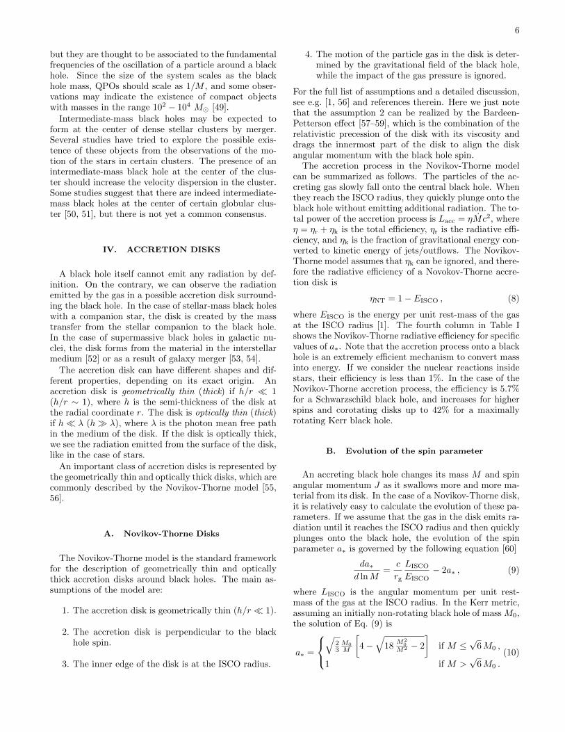
In the disk-corona model, a black hole accretes from ageometrically thin and optically thick accretion disk, seeFig. 4. The disk emits as a blackbody locally and as amulti-color blackbody when integrated radially4. For agiven radius of the disk, the temperature depends on theblack hole mass and the mass accretion rate. The peak

4 Every point in the accretion disk is in local thermal equilibrium,and therefore we can define an effective temperature Teff [in thecase of an axisymmetric system, Teff = Teff(r) depends only onthe radial coordinate]. Different points have a different tem-perature, and therefore we speak about “multi-color” or “multi-temperature” spectrum. The gas temperature increases as thegas particles fall into the gravitational potential of the black holeand transform potential energy into kinetic and internal energy.

Black HoleAccretion Disk

CoronaThermal

Component ReflectionComponent

Power-LawComponent

FIG. 4. Disk-corona model. The black hole is surroundedby a thin accretion disk with a multi-color blackbody spec-trum (red arrows). Some thermal photons from the disk haveinverse Compton scattering off free electrons in the corona,producing a power-law component (blue arrows). The latteralso illuminates the disk, generating a reflection component(green arrows).

temperature is reached near the inner edge of the diskand is in the soft X-ray band (0.1 − 1 keV) for stellar-mass black holes and in the optical/UV band (1−10 eV)for supermassive black holes. The thermal component ofthe accretion disk is indicated by the red arrows in Fig. 4.

The corona is a hotter (∼ 100 keV), usually opticallythin, cloud close to the black hole, but its exact geom-etry is currently unknown. In the lamppost geometry,the corona is a point-like source along the spin axis ofthe black hole [70]. In the sandwich geometry, it is theatmosphere above the accretion disk [71]. The inverseCompton scattering of the thermal photons from the ac-cretion disk off free electrons in the corona produces apower-law component (blue arrows in Fig. 4) with a cut-off energy that depends on the temperature of the corona(Ecut ∼ 100− 1000 keV).

The power-law component from the corona illuminatesalso the accretion disk, producing a reflection component(green arrows in Fig. 4) with some fluorescent emissionlines [72]. The strongest feature of the reflection compo-nent is usually the iron Kα line, which is at 6.4 keV inthe case of neutral or weakly ionized iron and shifts upto 6.97 keV for H-like iron ions.

A. Spectral States

An accreting black hole can be found in different “spec-tral states”, which are characterized by the luminosity ofthe source and by the relative contribution of its spec-tral components (thermal, power-law, reflection) [73, 74].The spectral state classification is purely phenomenologi-

8

cal, i.e. follows from the observed X-ray spectrum. How-ever, there should be a correlation (not completely un-derstood as of now) between spectral states and accretionflow configurations.

Let us start discussing the case of a stellar-mass blackhole in an X-ray transient. The object typically spendsmost of the time in a quiescent state with a very low ac-cretion luminosity (L/LEdd < 10−6). At a certain point,the source has an outburst and becomes a bright X-raysource in the sky (L/LEdd ∼ 10−3 − 1). The quiescentstate is determined by a very low mass accretion rate,namely a very low amount of material transfers from thecompanion star to the black hole. When there is a sud-den increase of the mass accretion rate (for instance, thecompanion star inflates and the black hole strips materialfrom the surface of the companion), there is the outburst.The object may be in a quiescent state for several monthsor even decades. An outburst typically lasts from somedays to a few months (roughly the time that the blackhole takes to swallow the material that produced the out-burst). During an outburst, the spectrum of the sourcechanges.

The hardness-intensity diagram (HID) [73, 74] is a use-ful tool for the description of an outburst, see Fig. 5. Thex-axis is for the hardness of the source, which is the ra-tio between its luminosity in the hard and soft X-raybands, for instance between the luminosity in the 6− 10and 2 − 6 keV bands, but other choices are also com-mon. The y-axis can be for the X-ray luminosity or thecount number of the instrument, but other choices arealso possible. The hardness-intensity diagram dependson the source (e.g. the interstellar absorption) and onthe instrument (e.g. its effective area at different ener-gies), but, despite that, it turns out to be very useful tostudy transient sources.

The relation between spectral states and accretion flowcan be understood noting that the intensity of the ther-mal component is mainly determined by the mass ac-cretion rate and the position of the inner edge of theaccretion disk, while the contributions of the power-lawand reflection components depend on the properties ofthe corona (its location, extension, geometry, etc.). Inparticular, the local flux of the disk’s thermal compo-nent is approximately proportional to the mass accre-tion rate and the inverse of the cube of the disk’s ra-dius, F(r) ∝ M/r3 [75]. When the mass accretion rateis low (high) and the inner edge of the disk is at large(small) radii, the thermal component is weak (strong).The power-law and the reflection components are strong(weak) when the corona is large (small) and close to (farfrom) the disk. The relative contribution of these threecomponents depends on the material around the blackhole, and, in turn, determines the spectral state.

Quiescent state — The source is initially in a quiescentstate: the mass accretion rate and the luminosity are verylow (the source may also be too faint to be detected) andthe spectrum is hard. The inner edge of the accretiondisk is truncated at a radius significantly larger than the

radius of the ISCO.Hard state — At the beginning of the outburst,

the spectrum is hard and the source becomes brighterand brighter because the mass accretion rate increases(L/LEdd starts from ∼ 10−3 and can reach values up to∼ 0.7 in some cases). The spectrum is dominated by thepower-law and reflection components. The thermal com-ponent is subdominant, and the temperature of the innerpart of the disk may be low, around 0.1 keV or even lower,but it increases as the luminosity of the source rises. Theinner edge of the disk is initially at a radius larger thanthe ISCO one, but it moves to the ISCO as the lumi-nosity increases (as shown in Fig. 5, where the disk is inblack), and it may be at the ISCO at the end of the hardstate. During the hard state, compact mildly relativisticsteady jets (in violet in Fig. 5) are common, but the exactmechanism producing these jets is currently unknown.Intermediate states — The power-law and the reflec-

tion components get weaker, probably because of a vari-ation in the geometry/properties of the corona. As aconsequence, the contribution of the thermal componentincreases and the source moves to the left part of theHID. We first have the hard-intermediate state and thenthe soft-intermediate state. As shown in Fig. 5, thereexists a jet line, not well understood for the moment, inthe HID: when the source crosses the jet line, we observetransient highly relativistic jets. Even in this case, themechanism responsible for the production of these jetsis unknown. If the hardness of the source oscillates nearthe jet line, we can observe several transient jets.Soft state — The thermal spectrum of the disk is the

dominant component in the spectrum and the inner partof the disk temperature is around 1 keV. If the luminosityof the source is between 5% to 30% of its Eddington

X-R

a y L

um

ino

sity

Quiescent State

Hardness

Hard State

Soft State

Hard-IntermediateState

Jet LineSoft-IntermediateState

Jet Line ?

FIG. 5. Evolution of the prototype of an outburst in thehardness-intensity diagram. The source is initially in a quies-cent state. At the beginning of the outburst, the source entersthe hard state, then moves to some intermediate states, to thesoft state, and eventually returns to a quiescent state. See thetext for more details.

9

luminosity, the inner edge of the disk should be at theISCO radius [76]. In the soft state, we do not observeany kind of jet5. However, strong winds and outflows arecommon (while they are absent in the hard state). Theluminosity of the source may somewhat decreases andchanges hardness, remaining on the left side of the HID.

At a certain point, the transfer of material decreases,leading to the end of the outburst. The contributionof the thermal spectrum of the disk decreases and, as aconsequence, the hardness of the source increases. Thesource re-enters the soft-intermediate state, the hard-intermediate state, then the hard state, and eventually,when the hardness is high, the luminosity drops downand the source returns to the quiescent state till the nextoutburst. Between the soft-intermediate and the hard-intermediate states, we may observe transient jets, butthe existence of a jet line is not clear here. Every sourcefollows the path shown in Fig. 5 counter-clockwise, butthere are differences among different sources and even forthe same source among different outbursts.

In the case of stellar-mass black holes in persistent X-ray sources, there is no outburst, but we can still use theHID. The most studied source is Cygnus X-1 (the otherpersistent sources are in nearby galaxies, so they arefainter and more difficult to study). This object spendsmost of the time in the hard state, but it occasionallymoves to a softer state, which is usually interpreted as asoft state. LMC X-1 is always in the soft state. LMC X-3is usually observed in the soft state, rarely in the hardstate, and there is no clear evidence that this source canbe in an intermediate state.

In the case of supermassive black holes, there are atleast two important differences. First, the size of thesystem, which scales as the mass. 1 day for a 10 M�black hole corresponds to 3,000 years for a 107 M� blackhole, which makes impossible the study of the evolutionof a specific system. Second, the temperature of the diskis in the optical/UV range for a supermassive black hole.Despite these two issues, stellar-mass and supermassiveblack holes have a similar behavior and we can employthe same spectral state classification (see, for instance,[73] and references therein).

VI. TECHNIQUES FOR PROBING THESTRONG GRAVITY REGION

The aim of this section is to describe the leading tech-niques to probe the strong gravity region around blackholes. The continuum-fitting method and X-ray reflec-tion spectroscopy are well-established electromagnetic

5 For instance, in the corona lamppost geometry, the corona maybe the base of the jet. This could explain why, in the soft state,we do not see jets and the power-law and reflection componentsare weak.

approaches. The measurement of quasi-periodic oscil-lations is not yet a mature technique, because severalmodels have been proposed but we do not know whichone, if any, is correct. Direct imaging of the accretionflow will be possible very soon for SgrA∗, the supermas-sive black hole at the center of our Galaxy. Gravitationalwaves are a recent new tool that promises a huge amountof completely new data in the next years.

A. Continuum-Fitting Method

Within the Novikov-Thorne model [55, 56], we can de-rive the time-averaged radial structure of the accretiondisk from the fundamental laws of the conservation ofrest-mass, energy, and angular momentum. The time-averaged energy flux emitted from the surface of the diskis

F(r) =Mc2

4πr2g

F (r) , (12)

where M = dM/dt is the time-averaged mass accretionrate, which is independent of the radial coordinate, andF (r) is a dimensionless function of the radial coordinatethat becomes roughly of order 1 at the disk inner edge(see [56] for more details). Assuming that the disk is inlocal thermal equilibrium, its emission is blackbody-likeand at any radius we can define an effective temperatureTeff(r) from the time-averaged energy flux as F = σT 4

eff ,where σ is the Stefan-Boltzmann constant.

Novikov-Thorne disks with the inner edge at the ISCOradius are realized when the accretion luminosity is be-tween 5% to 30% of the Eddington limit of the object [76],and this is confirmed by theoretical [77, 78] and obser-vational studies [79]. At lower luminosities, the disk ismore likely truncated. At higher luminosities, the gaspressure becomes important, the inner part of the diskis not thin any longer, and the inner edge might be at aradius smaller than the ISCO. Requiring M ∼ 0.1 MEdd

as the condition for Novikov-Thorne disks, we can get arough estimate of the effective temperature of the innerpart of the accretion disk

Teff ∼

(0.1 MEddc

2

4πσr2g

)1/4

∼(

10 M�

M

)1/4

keV , (13)

and we can see that the disk’s thermal spectrum is in thesoft X-ray band for stellar-mass black holes and in theoptical/UV band for the supermassive one.

The continuum-fitting method is the analysis of thethermal spectrum of geometrically thin and opticallythick accretion disks of black holes in order to measurethe black hole spin parameter a∗ [80–83]. The techniqueis normally used for stellar-mass black holes only, becausethe spectrum of supermassive black holes is in the opti-cal/UV band where dust absorption limits the capabilityof accurate measurements.

10

The model describing the thermal spectrum of an ac-cretion disk around a Kerr black holes depends on fiveparameters: the black hole mass M , the mass accretionrate M , the inclination angle of the disk i, the distance ofthe source from the observer D, and the black hole spinparameter a∗. It is not possible to infer all these parame-ters from the data of the spectrum of a thin disk, becausethere is a degeneracy. However, if we can get indepen-dent measurements of M , D, and i, usually from opticalobservations, it is possible to fit the thermal componentand measure a∗ and M . This is the continuum-fittingmethod. Currently, there are about ten stellar-massblack holes with a spin measurement from the continuum-fitting method, see Tab. II.

B. X-Ray Reflection Spectroscopy

X-ray reflection spectroscopy (or iron line method)refers to the study of the reflection component. Thistechnique can be applied to both stellar-mass and su-permassive black holes and is currently the only avail-able method to measure the spin of supermassive blackholes [112, 113].

The most prominent feature of the reflection spectrumis usually the iron Kα line. This is because the iron ismore abundant than other heavy elements (the iron-26nucleus is more tightly bound than lighter and heavierelements, so it is the final product of nuclear reactions)and the probability of fluorescent line emission is alsohigh. The iron Kα line is a very narrow feature in therest-frame of the emitter, while the one observed in thereflection spectrum of black holes can be very broad andskewed, as the result of relativistic effects occurring in thestrong gravity region of the object (gravitational redshift,Doppler boosting, light bending) [1, 112–114]. While theiron Kα line is usually the strongest feature, accuratemeasurements of black hole spins require to fit the wholereflection spectrum, not just the iron line.

Reflection models describing the reflection componentof accretion disks around Kerr black holes depend on sev-eral parameters: the black holes spin a∗, the inner edgeof the disk Rin (which may or may not be at the ISCO ra-dius, see the discussion in Section V A), the outer edge ofthe disk Rout, the inclination angle of the disk i, the ironabundance AFe, the ionization of the disk ξ, and someparameters related to the emissivity profile of the disk.The latter is quite a crucial ingredient and depends onthe geometry of the corona, which is currently unknown.Coronas with arbitrary geometries can be modeled witha power-law emissivity profile (the intensity on the diskis I ∝ 1/rq where q is the emissivity index) or with abroken power-law (I ∝ 1/rqin for r < Rbr, I ∝ 1/rqout

for r > Rbr, and we have three parameters: the inneremissivity index qin, the outer emissivity index qout, andthe breaking radius Rbr). In the case of supermassiveblack holes, it is often necessary to take the cosmologi-cal redshift z into account. For stellar-mass black holes,

their relative motion in the Galaxy is of order 100 km/sand their Doppler boosting can be ignored.

Note that spin measurements with the iron line methoddo not require independent measurements of the blackhole mass M , the distance D, and the inclination angleof the disk i, three quantities that are required in thecontinuum-fitting method, are usually difficult to mea-sure, and have large uncertainty. The reflection spectrumis independent of M and D, and can directly measure theinclination angle of the disk i.

Current spin measurements of stellar-mass black holeswith the iron line method are summarized in the thirdcolumn in Tab. II (see the corresponding references in thefourth column for more details). Note that some blackholes have their spin measured with both the continuum-fitting and the iron line methods. In general, the twomeasurements agree (GRS 1915+105, Cyg X-1, LMC X-1, XTE J1550-564). For GX 339-4 and GRO J1655-40,the two measurements are not consistent. The iron linemethod is usually applied when the source is in the hardstate, when the reflection spectrum is stronger but thedisk may be truncated at a radius larger than the ISCO.This would lead to underestimate the black hole spin,and therefore it cannot be the case of the spin mea-surements of GX 339-4 and GRO J1655-40, where theiron line method provides spin values higher than thecontinuum-fitting method. As pointed out before, thecontinuum-fitting method crucially depends on indepen-dent measurements of the black hole mass M , the dis-tance D, and the inclination angle of the disk i, threequantities that are usually difficult to measure and maybe affected by systematic effects. For example, in thecase of GRO J1655-40 there are a few mass measure-ments reported in the literature, but they are not consis-tent among them.

A summary of spin measurements of supermassiveblack holes with the iron line method is reported inTab. III (see the references in the last column for more de-tails and the lists of spin measurements in [112, 113, 130]for a few more sources with a constrained spin). Note thevery high spin of several objects. In part, this can be ex-plained noting that fast-rotating black holes are brighterand thus the spin measurement is easier. If these mea-surements are correct, they would point out that theseobjects have been spun up by prolonged disk accretionand therefore would provide information about galaxyevolutions (see the discussion in Section IV B). However,the very high spin measurements have to be taken withsome caution, as they may be affected by systematic ef-fects in the model employed to infer the black hole spin.More details on the possible interpretation of current spinmeasurements of supermassive black holes can be foundin [112].

11

BH Binary a∗ (Continuum) a∗ (Iron) Principal References

GRS 1915+105 > 0.98 0.98 ± 0.01 [76, 84]

Cyg X-1 > 0.98 0.97+0.014−0.02 [85–90]

GS 1354-645 – > 0.98 [91]

LMC X-1 0.92 ± 0.06 0.97+0.02−0.25 [92, 93]

GX 339-4 < 0.9 0.95 ± 0.03 [94–97]

MAXI J1836-194 — 0.88 ± 0.03 [98]

M33 X-7 0.84 ± 0.05 — [99]

4U 1543-47 0.80 ± 0.10? — [100]

IC10 X-1 >∼ 0.7 — [101]

Swift J1753.5 — 0.76+0.11−0.15 [102]

XTE J1650-500 — 0.84 ∼ 0.98 [103]

GRO J1655-40 0.70 ± 0.10? > 0.9 [100, 102]

GS 1124-683 0.63+0.16−0.19 — [104]

XTE J1752-223 — 0.52 ± 0.11 [105]

XTE J1652-453 — < 0.5 [106]

XTE J1550-564 0.34 ± 0.28 0.55+0.15−0.22 [107]

LMC X-3 0.25 ± 0.15 — [108]

H1743-322 0.2 ± 0.3 — [110]

A0620-00 0.12 ± 0.19 — [109]

XMMU J004243.6 < −0.2 — [111]

TABLE II. Summary of the continuum-fitting and iron line measurements of the spin parameter of stellar-mass black holes. Seethe references in the last column for more details. Note: ?These sources were studied in an early work of the continuum-fittingmethod, within a more simple model, and therefore the published 1-σ error estimates are doubled following [83].

C. Quasi-Periodic Oscillations

Quasi-periodic oscillations (QPOs) are a common fea-ture in the X-ray power density spectrum of neutron starsand stellar-mass black holes [131]. The power densityspectrum P (ν) is the square of the Fourier transform ofthe photon count rate C(t). If we use the Leahy normal-ization, we have

P (ν) =2

N

∣∣∣∣∣∫ T

0

C(t)e−2πiνtdt

∣∣∣∣∣ , (14)

where N is the total number of counts and T is the du-ration of the observation. QPOs are narrow features inthe X-ray power density spectrum of a source. Fig. 6shows the power density spectrum obtained from an ob-servation of the stellar-mass black hole XTE J11550-564,where we can see a QPO around 5 Hz, one at 13 Hz, andone at 183 Hz in the inset.

In the case of black hole binaries, QPOs can be groupedinto two classes: low-frequency QPOs (0.1− 30 Hz) andhigh-frequency QPOs (40−450 Hz). The exact nature ofthese QPOs is currently unknown, but there are severalproposals in literature. In most scenarios, the frequen-cies of the QPOs is somehow related to the fundamentalfrequencies of a particle orbiting the black hole [133–135]:

1. Orbital frequency νφ, which is the inverse of theorbital period.

2. Radial epicyclic frequency νr, which is the fre-quency of radial oscillations around the mean orbit.

3. Vertical epicyclic frequency νθ, which is the fre-quency of vertical oscillations around the mean or-bit.

In the Kerr metric, we have a compact analytic form

10−1 100 101

101

Pow

er s

pect

ral d

ensi

ty

Frequency (Hz)

100 400 10001.55

1.6

1.65

1.7

1.75

Pow

er s

pect

ral d

ensi

ty

Frequency (Hz)

183 Hz

13 Hz

FIG. 6. Power density spectrum from an observation ofXTE J1550-564. We see a QPO around 5 Hz, a QPO at13 Hz (marked by an arrow), and a QPO at 183 Hz in theinset (marked by an arrow). Fig. 1 from [132], reproduced bypermission of Oxford University Press.

12

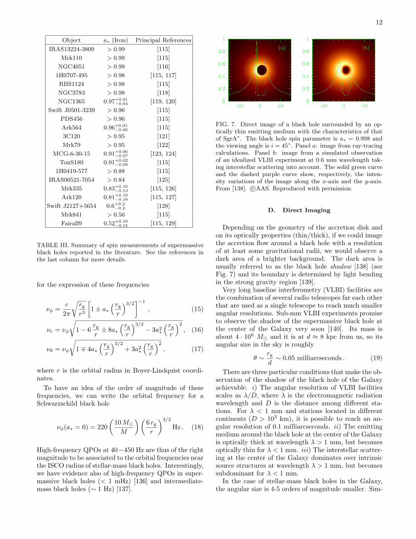
Object a∗ (Iron) Principal References

IRAS13224-3809 > 0.99 [115]

Mrk110 > 0.99 [115]

NGC4051 > 0.99 [116]

1H0707-495 > 0.98 [115, 117]

RBS1124 > 0.98 [115]

NGC3783 > 0.98 [118]

NGC1365 0.97+0.01−0.04 [119, 120]

Swift J0501-3239 > 0.96 [115]

PDS456 > 0.96 [115]

Ark564 0.96+0.01−0.06 [115]

3C120 > 0.95 [121]

Mrk79 > 0.95 [122]

MCG-6-30-15 0.91+0.06−0.07 [123, 124]

TonS180 0.91+0.02−0.09 [115]

1H0419-577 > 0.88 [115]

IRAS00521-7054 > 0.84 [125]

Mrk335 0.83+0.10−0.13 [115, 126]

Ark120 0.81+0.10−0.18 [115, 127]

Swift J2127+5654 0.6+0.2−0.2 [128]

Mrk841 > 0.56 [115]

Fairall9 0.52+0.19−0.15 [115, 129]

TABLE III. Summary of spin measurements of supermassiveblack holes reported in the literature. See the references inthe last column for more details.

for the expression of these frequencies

νφ =c

2π

√rg

r3

[1± a∗

(rg

r

)3/2]−1

, (15)

νr = νφ

√1− 6

rg

r± 8a∗

(rg

r

)3/2

− 3a2∗

(rg

r

)2

, (16)

νθ = νφ

√1∓ 4a∗

(rg

r

)3/2

+ 3a2∗

(rg

r

)2

, (17)

where r is the orbital radius in Boyer-Lindquist coordi-nates.

To have an idea of the order of magnitude of thesefrequencies, we can write the orbital frequency for aSchwarzschild black hole

νφ(a∗ = 0) = 220

(10M�

M

)(6 rg

r

)3/2

Hz . (18)

High-frequency QPOs at 40−450 Hz are thus of the rightmagnitude to be associated to the orbital frequencies nearthe ISCO radius of stellar-mass black holes. Interestingly,we have evidence also of high-frequency QPOs in super-massive black holes (< 1 mHz) [136] and intermediate-mass black holes (∼ 1 Hz) [137].

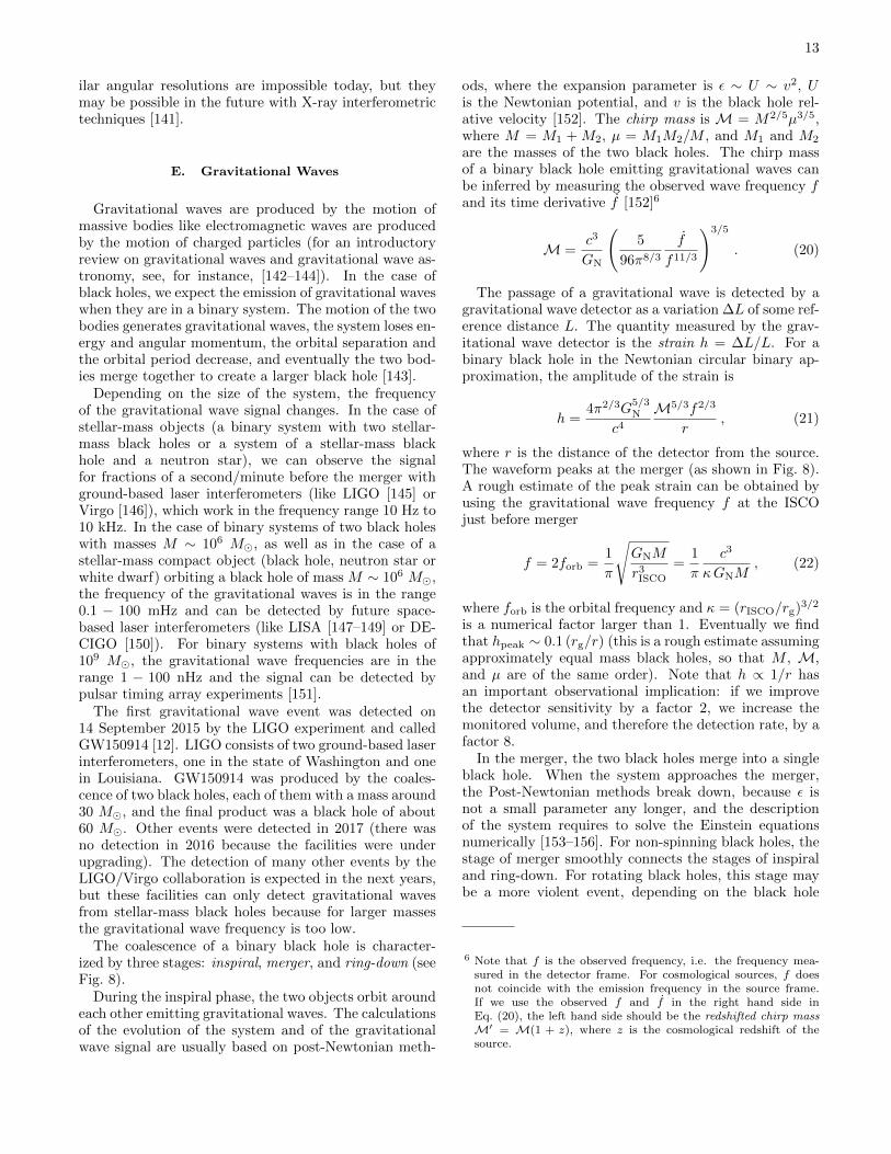
FIG. 7. Direct image of a black hole surrounded by an op-tically thin emitting medium with the characteristics of thatof SgrA∗. The black hole spin parameter is a∗ = 0.998 andthe viewing angle is i = 45◦. Panel a: image from ray-tracingcalculations. Panel b: image from a simulated observationof an idealized VLBI experiment at 0.6 mm wavelength tak-ing interstellar scattering into account. The solid green curveand the dashed purple curve show, respectively, the inten-sity variations of the image along the x-axis and the y-axis.From [138]. c©AAS. Reproduced with permission.

D. Direct Imaging

Depending on the geometry of the accretion disk andon its optically properties (thin/thick), if we could imagethe accretion flow around a black hole with a resolutionof at least some gravitational radii, we would observe adark area of a brighter background. The dark area isusually referred to as the black hole shadow [138] (seeFig. 7) and its boundary is determined by light bendingin the strong gravity region [139].

Very long baseline interferometry (VLBI) facilities arethe combination of several radio telescopes far each otherthat are used as a single telescope to reach much smallerangular resolutions. Sub-mm VLBI experiments promiseto observe the shadow of the supermassive black hole atthe center of the Galaxy very soon [140]. Its mass isabout 4 · 106 M� and it is at d ≈ 8 kpc from us, so itsangular size in the sky is roughly

θ ∼ rg

d∼ 0.05 milliarcseconds . (19)

There are three particular conditions that make the ob-servation of the shadow of the black hole of the Galaxyachievable. i) The angular resolution of VLBI facilitiesscales as λ/D, where λ is the electromagnetic radiationwavelength and D is the distance among different sta-tions. For λ < 1 mm and stations located in differentcontinents (D > 103 km), it is possible to reach an an-gular resolution of 0.1 milliarcseconds. ii) The emittingmedium around the black hole at the center of the Galaxyis optically thick at wavelength λ > 1 mm, but becomesoptically thin for λ < 1 mm. iii) The interstellar scatter-ing at the center of the Galaxy dominates over intrinsicsource structures at wavelength λ > 1 mm, but becomessubdominant for λ < 1 mm.

In the case of stellar-mass black holes in the Galaxy,the angular size is 4-5 orders of magnitude smaller. Sim-

13

ilar angular resolutions are impossible today, but theymay be possible in the future with X-ray interferometrictechniques [141].

E. Gravitational Waves

Gravitational waves are produced by the motion ofmassive bodies like electromagnetic waves are producedby the motion of charged particles (for an introductoryreview on gravitational waves and gravitational wave as-tronomy, see, for instance, [142–144]). In the case ofblack holes, we expect the emission of gravitational waveswhen they are in a binary system. The motion of the twobodies generates gravitational waves, the system loses en-ergy and angular momentum, the orbital separation andthe orbital period decrease, and eventually the two bod-ies merge together to create a larger black hole [143].

Depending on the size of the system, the frequencyof the gravitational wave signal changes. In the case ofstellar-mass objects (a binary system with two stellar-mass black holes or a system of a stellar-mass blackhole and a neutron star), we can observe the signalfor fractions of a second/minute before the merger withground-based laser interferometers (like LIGO [145] orVirgo [146]), which work in the frequency range 10 Hz to10 kHz. In the case of binary systems of two black holeswith masses M ∼ 106 M�, as well as in the case of astellar-mass compact object (black hole, neutron star orwhite dwarf) orbiting a black hole of mass M ∼ 106 M�,the frequency of the gravitational waves is in the range0.1 − 100 mHz and can be detected by future space-based laser interferometers (like LISA [147–149] or DE-CIGO [150]). For binary systems with black holes of109 M�, the gravitational wave frequencies are in therange 1 − 100 nHz and the signal can be detected bypulsar timing array experiments [151].

The first gravitational wave event was detected on14 September 2015 by the LIGO experiment and calledGW150914 [12]. LIGO consists of two ground-based laserinterferometers, one in the state of Washington and onein Louisiana. GW150914 was produced by the coales-cence of two black holes, each of them with a mass around30 M�, and the final product was a black hole of about60 M�. Other events were detected in 2017 (there wasno detection in 2016 because the facilities were underupgrading). The detection of many other events by theLIGO/Virgo collaboration is expected in the next years,but these facilities can only detect gravitational wavesfrom stellar-mass black holes because for larger massesthe gravitational wave frequency is too low.

The coalescence of a binary black hole is character-ized by three stages: inspiral, merger, and ring-down (seeFig. 8).

During the inspiral phase, the two objects orbit aroundeach other emitting gravitational waves. The calculationsof the evolution of the system and of the gravitationalwave signal are usually based on post-Newtonian meth-

ods, where the expansion parameter is ε ∼ U ∼ v2, Uis the Newtonian potential, and v is the black hole rel-ative velocity [152]. The chirp mass is M = M2/5µ3/5,where M = M1 + M2, µ = M1M2/M , and M1 and M2

are the masses of the two black holes. The chirp massof a binary black hole emitting gravitational waves canbe inferred by measuring the observed wave frequency fand its time derivative f [152]6

M =c3

GN

(5

96π8/3

f

f11/3

)3/5

. (20)

The passage of a gravitational wave is detected by agravitational wave detector as a variation ∆L of some ref-erence distance L. The quantity measured by the grav-itational wave detector is the strain h = ∆L/L. For abinary black hole in the Newtonian circular binary ap-proximation, the amplitude of the strain is

h =4π2/3G

5/3N

c4M5/3f2/3

r, (21)

where r is the distance of the detector from the source.The waveform peaks at the merger (as shown in Fig. 8).A rough estimate of the peak strain can be obtained byusing the gravitational wave frequency f at the ISCOjust before merger

f = 2forb =1

π

√GNM

r3ISCO

=1

π

c3

κGNM, (22)

where forb is the orbital frequency and κ = (rISCO/rg)3/2

is a numerical factor larger than 1. Eventually we findthat hpeak ∼ 0.1 (rg/r) (this is a rough estimate assumingapproximately equal mass black holes, so that M , M,and µ are of the same order). Note that h ∝ 1/r hasan important observational implication: if we improvethe detector sensitivity by a factor 2, we increase themonitored volume, and therefore the detection rate, by afactor 8.

In the merger, the two black holes merge into a singleblack hole. When the system approaches the merger,the Post-Newtonian methods break down, because ε isnot a small parameter any longer, and the descriptionof the system requires to solve the Einstein equationsnumerically [153–156]. For non-spinning black holes, thestage of merger smoothly connects the stages of inspiraland ring-down. For rotating black holes, this stage maybe a more violent event, depending on the black hole

6 Note that f is the observed frequency, i.e. the frequency mea-sured in the detector frame. For cosmological sources, f doesnot coincide with the emission frequency in the source frame.If we use the observed f and f in the right hand side inEq. (20), the left hand side should be the redshifted chirp massM′ = M(1 + z), where z is the cosmological redshift of thesource.

14

FIG. 8. Temporal evolution of the strain, the black holeseparation, and the black hole relative velocity in the eventGW150914. From [12] under the terms of the Creative Com-mons Attribution 3.0 License.

spins and their alignments with respect to the orbitalangular momentum.

Lastly, the newly-born black hole emits gravitationalwaves to settle down to an equilibrium configuration.This is the ring-down stage, which is commonly describedby black hole perturbation theory [17, 157]. The gravi-tational wave signal is characterized by damped oscilla-tions, the so-called quasi-normal modes [158–160]. Thisis not a special property of black holes, and it is ex-pected even in neutron stars or other possible compactself-gravitating systems (e.g. boson stars, wormholes,etc). However, the frequency and the damping time ofthese oscillations do depend on the specific system and itsproperties, while they are independent of the initial per-turbations. In the case of a Schwarzschild black hole, thespectrum of the quasi-normal modes is only determined

by the black hole mass. The frequency and the dampingtime of the dominant quasi-normal mode are [160]

f = 1.207

(10M�

M

)kHz ,

τ = 0.554

(M

10M�

)ms . (23)

For a Kerr black hole, the spectrum depends on the massM and the spin parameter a∗.

VII. CONCLUDING REMARKS

This article has briefly reviewed the state of the art ofthe study of astrophysical black holes, starting from theirkey-properties predicted in general relativity and summa-rizing current observations and techniques to probe thestrong gravitational field of these objects. The referencesprovided in each section should serve as the next step forthe reader interested to know more on specific topics.

The past 10-20 years have seen significant progressesin the understanding of these systems, and we can ex-pect much more progresses in the near future, thanksto the detection of a large number of gravitationalwave events, the next generation of X-ray facilities (likeeXTP [161, 162] and Athena [163]), and the observa-tion of the shadow of the black hole at the center of ourGalaxy with sub-mm VLBI experiments. While in thepast this research field was studied only by astronomers,there is now an increasing interest from the physics com-munity, because observational data are now reaching alevel that it is possible to test fundamental physics, inparticular general relativity and alternative theories ofgravity [164, 165]. There are also arguments suggestingthat astrophysical black holes may be macroscopic quan-tum objects, and that we might be able to detect signa-tures of quantum gravity from their observations [166].

ACKNOWLEDGMENTS

The author acknowledges support from theNational Natural Science Foundation of China(Grant No. U1531117), Fudan University (GrantNo. IDH1512060), and the Alexander von HumboldtFoundation.

[1] C. Bambi, Black Holes: A Laboratory for Testing StrongGravity (Springer Singapore, 2017), doi:10.1007/978-981-10-4524-0

[2] A. Einstein, Annalen Phys. 49, 769 (1916) [AnnalenPhys. 14, 517 (2005)].

[3] K. Schwarzschild, Sitzungsber. Preuss. Akad.Wiss. Berlin (Math. Phys. ) 1916, 189 (1916)[physics/9905030].

[4] D. Finkelstein, Phys. Rev. 110, 965 (1958).[5] R. P. Kerr, Phys. Rev. Lett. 11, 237 (1963).

[6] Y. B. Zeldovich, Dokl. Akad. Nauk 155, 67 (1964) [Sov.Phys. Dokl. 9, 195 (1964)].

[7] E. E. Salpeter, Astrophys. J. 140, 796 (1964).[8] C. T. Bolton, Nature 235, 271 (1972).[9] B. L. Webster and P. Murdin, Nature 235, 37 (1972).

[10] R. A. Remillard and J. E. McClintock, Ann. Rev. As-tron. Astrophys. 44, 49 (2006) [astro-ph/0606352].

[11] J. Kormendy and D. Richstone, Ann. Rev. Astron. As-trophys. 33, 581 (1995).

[12] B. P. Abbott et al. [LIGO Scientific and Virgo Col-

15

laborations], Phys. Rev. Lett. 116, 061102 (2016)[arXiv:1602.03837 [gr-qc]].

[13] W. Israel, Phys. Rev. 164, 1776 (1967).[14] B. Carter, Phys. Rev. Lett. 26, 331 (1971).[15] D. C. Robinson, Phys. Rev. Lett. 34, 905 (1975).[16] P. T. Chrusciel, J. L. Costa and M. Heusler, Living Rev.

Rel. 15, 7 (2012) [arXiv:1205.6112 [gr-qc]].[17] S. Chandrasekhar, The Mathematical Theory of Black

Holes (Clarendon Press, Oxford, UK, 1998).[18] C. W. Misner, K. S. Thorne and J. A. Wheeler, Grav-

itation (W. H. Freeman and Company, San Francisco,California, 1973).

[19] M. Coleman Miller and E. J. M. Colbert, Int. J. Mod.Phys. D 13, 1 (2004) [arXiv:astro-ph/0308402].

[20] C. E. Rhoades and R. Ruffini, Phys. Rev. Lett. 32, 324(1974).

[21] V. Kalogera and G. Baym, Astrophys. J. 470, L61(1996).

[22] J. M. Lattimer, Ann. Rev. Nucl. Part. Sci. 62, 485(2012) [arXiv:1305.3510 [nucl-th]].

[23] W. M. Farr, N. Sravan, A. Cantrell, L. Kreidberg,C. D. Bailyn, I. Mandel and V. Kalogera, Astrophys.J. 741, 103 (2011) [arXiv:1011.1459 [astro-ph.GA]].

[24] M. Y. Khlopov, Res. Astron. Astrophys. 10, 495 (2010)[arXiv:0801.0116 [astro-ph]].

[25] E. P. J. van den Heuvel, Endpoints of stellar evolution:The incidence of stellar mass black holes in the galaxy,in “Environment Observation and Climate ModellingThrough International Space Projects”, 29 (1992).

[26] F. X. Timmes, S. E. Woosley and T. A. Weaver, Astro-phys. J. 457, 834 (1996) [astro-ph/9510136].

[27] K. Belczynski, T. Bulik, C. L. Fryer, A. Ruiter,J. S. Vink and J. R. Hurley, Astrophys. J. 714, 1217(2010) [arXiv:0904.2784 [astro-ph.SR]].

[28] A. Heger and S. E. Woosley, Astrophys. J. 567, 532(2002) [astro-ph/0107037].

[29] A. Heger, C. L. Fryer, S. E. Woosley, N. Langer andD. H. Hartmann, Astrophys. J. 591, 288 (2003) [astro-ph/0212469].

[30] M. Spera, M. Mapelli and A. Bressan, Mon. Not. Roy.Astron. Soc. 451, no. 4, 4086 (2015) [arXiv:1505.05201[astro-ph.SR]].

[31] J. Casares and P. G. Jonker, Space Sci. Rev. 183, 223(2014) [arXiv:1311.5118 [astro-ph.HE]].

[32] L. R. Yungelson, J.-P. Lasota, G. Nelemans, G. Dubus,E. P. J. van den Heuvel, J. Dewi and S. Portegies Zwart,Astron. Astrophys. 454, 559 (2006) [astro-ph/0604434].

[33] P. D. Kiel and J. R. Hurley, Mon. Not. Roy. Astron.Soc. 369, 1152 (2006) [astro-ph/0605080].

[34] E. Agol, M. Kamionkowski, L. V. E. Koopmans andR. D. Blandford, Astrophys. J. 576, L131 (2002) [astro-ph/0203257].

[35] P. J. McMillan, Mon. Not. Roy. Astron. Soc. 465, 76(2017) [arXiv:1608.00971 [astro-ph.GA]].

[36] A. Boehle et al., Astrophys. J. 830, 17 (2016)[arXiv:1607.05726 [astro-ph.GA]].

[37] E. Maoz, Astrophys. J. 494, L181 (1998) [astro-ph/9710309].

[38] M. Postman et al., Astrophys. J. 756, 159 (2012)[arXiv:1205.3839 [astro-ph.CO]].

[39] M. Volonteri, Astron. Astrophys. Rev. 18, 279 (2010)[arXiv:1003.4404 [astro-ph.CO]].

[40] M. Volonteri, G. Lodato and P. Natarajan, Mon. Not.Roy. Astron. Soc. 383, 1079 (2008) [arXiv:0709.0529

[astro-ph]].[41] M. Volonteri, F. Haardt and K. Gultekin, Mon. Not.

Roy. Astron. Soc. 384, 1387 (2008) [arXiv:0710.5770[astro-ph]].

[42] L. Ferrarese et al., Astrophys. J. 644, L21 (2006) [astro-ph/0603840].

[43] E. Gallo, T. Treu, J. Jacob, J. H. Woo, P. Mar-shall and R. Antonucci, Astrophys. J. 680, 154 (2008)[arXiv:0711.2073 [astro-ph]].

[44] X.-B. Wu et al., Nature 518, 512 (2015).[45] P. Madau, F. Haardt and M. Dotti, Astrophys. J. 784,

L38 (2014) [arXiv:1402.6995 [astro-ph.CO]].[46] M. Bachetti et al., Nature 514, 202 [arXiv:1410.3590

[astro-ph.HE]].[47] E. J. M. Colbert and R. F. Mushotzky, Astrophys. J.

519, 89 (1999) [astro-ph/9901023].[48] K. Ohsuga and S. Mineshige, Astrophys. J. 736, 2

(2011) [arXiv:1105.5474 [astro-ph.HE]].[49] D. R. Pasham, T. E. Strohmayer and R. F. Mushotzky,

Nature 513, 74 (2014) [arXiv:1501.03180 [astro-ph.HE]].

[50] K. Gebhardt, R. M. Rich and L. C. Ho, Astrophys. J.578, L41 (2002) [astro-ph/0209313].

[51] K. Gebhardt, R. M. Rich and L. C. Ho, Astrophys. J.634, 1093 (2005) [astro-ph/0508251].

[52] I. Shlosman, M. C. Begelman and J. Frank, Nature 345,679 (1990).

[53] J. E. Barnes and L. Hernquist, Astrophys. J. 471, 115(1996).

[54] L. Mayer, S. Kazantzidis, P. Madau, M. Colpi,T. R. Quinn and J. Wadsley, Science 316, 1874 (2007)[arXiv:0706.1562 [astro-ph]].

[55] I. D. Novikov and K. S. Thorne, Astrophysics andblack holes, in Black Holes, edited by C. De Witt andB. De Witt (Gordon and Breach, New York, New York,1973).

[56] D. N. Page and K. S. Thorne, Astrophys. J. 191, 499(1974).

[57] J. M. Bardeen and J. A. Petterson, Astrophys. J. 195,L65 (1975).

[58] S. Kumar and J. E. Pringle, Mon. Not. Roy. Astron.Soc. 213, 435 (1985).

[59] J. F. Steiner and J. E. McClintock, Astrophys. J. 745,136 (2012) [arXiv:1110.6849 [astro-ph.HE]].

[60] K. S. Thorne, Astrophys. J. 191, 507 (1974).[61] A. R. King and U. Kolb, Mon. Not. Roy. Astron. Soc.

305, 654 (1999) [astro-ph/9901296].[62] T. Fragos and J. E. McClintock, Astrophys. J. 800, 17

(2015) [arXiv:1408.2661 [astro-ph.HE]].[63] E. Berti and M. Volonteri, Astrophys. J. 684, 822 (2008)

[arXiv:0802.0025 [astro-ph]].[64] S. A. Hughes and R. D. Blandford, Astrophys. J. 585,

L101 (2003) [astro-ph/0208484].[65] A. R. King and J. E. Pringle, Mon. Not. Roy. Astron.

Soc. 373, L93 (2006) [astro-ph/0609598].[66] E. Barausse, Mon. Not. Roy. Astron. Soc. 423, 2533

(2012) [arXiv:1201.5888 [astro-ph.CO]].[67] M. Dotti, M. Colpi, S. Pallini, A. Perego and M. Volon-

teri, Astrophys. J. 762, 68 (2013) [arXiv:1211.4871[astro-ph.CO]].

[68] A. Sesana, E. Barausse, M. Dotti and E. M. Rossi,Astrophys. J. 794, 104 (2014) [arXiv:1402.7088 [astro-ph.CO]].

[69] Y. Dubois, M. Volonteri and J. Silk, Mon. Not. Roy.

16

Astron. Soc. 440, no. 2, 1590 (2014) [arXiv:1304.4583[astro-ph.CO]].

[70] T. Dauser, J. Garcia, J. Wilms, M. Bock, L. W. Bren-neman, M. Falanga, K. Fukumura and C. S. Reynolds,Mon. Not. Roy. Astron. Soc. 430, 1694 (2013)[arXiv:1301.4922 [astro-ph.HE]].

[71] F. Haardt and L. Maraschi, Astrophys. J. 413, 507(1993).

[72] J. Garcia, T. Dauser, C. S. Reynolds, T. R. Kall-man, J. E. McClintock, J. Wilms and W. Eikmann,Astrophys. J. 768, 146 (2013) [arXiv:1303.2112 [astro-ph.HE]].

[73] T. M. Belloni, Lect. Notes Phys. 794, 53 (2010)[arXiv:0909.2474 [astro-ph.HE]].

[74] J. Homan and T. Belloni, Astrophys. Space Sci. 300,107 (2005) [astro-ph/0412597].

[75] J. P. Lasota, Black hole accretion discs,doi:10.1007/978-3-662-52859-4 1 arXiv:1505.02172[astro-ph.HE].

[76] J. E. McClintock, R. Shafee, R. Narayan, R. A. Remil-lard, S. W. Davis and L. X. Li, Astrophys. J. 652, 518(2006) [astro-ph/0606076].

[77] R. F. Penna, J. C. McKinney, R. Narayan,A. Tchekhovskoy, R. Shafee and J. E. McClintock, Mon.Not. Roy. Astron. Soc. 408, 752 (2010) [arXiv:1003.0966[astro-ph.HE]].

[78] A. K. Kulkarni et al., Mon. Not. Roy. Astron. Soc. 414,1183 (2011) [arXiv:1102.0010 [astro-ph.HE]].

[79] J. F. Steiner, J. E. McClintock, R. A. Remillard, L. Gou,S. Yamada and R. Narayan, Astrophys. J. 718, L117(2010) [arXiv:1006.5729 [astro-ph.HE]].

[80] S. N. Zhang, W. Cui and W. Chen, Astrophys. J. 482,L155 (1997) [astro-ph/9704072].

[81] L. X. Li, E. R. Zimmerman, R. Narayan and J. E. Mc-Clintock, Astrophys. J. Suppl. 157, 335 (2005) [astro-ph/0411583].

[82] J. E. McClintock et al., Class. Quant. Grav. 28, 114009(2011) [arXiv:1101.0811 [astro-ph.HE]].

[83] J. E. McClintock, R. Narayan and J. F. Steiner, SpaceSci. Rev. 183, 295 (2014) [arXiv:1303.1583 [astro-ph.HE]].

[84] J. M. Miller et al., Astrophys. J. 775, L45 (2013)[arXiv:1308.4669 [astro-ph.HE]].

[85] L. Gou et al., Astrophys. J. 742, 85 (2011)[arXiv:1106.3690 [astro-ph.HE]].

[86] L. Gou et al., Astrophys. J. 790, 29 (2014)[arXiv:1308.4760 [astro-ph.HE]].

[87] A. C. Fabian et al., Mon. Not. Roy. Astron. Soc. 424,217 (2012) [arXiv:1204.5854 [astro-ph.HE]].

[88] J. A. Tomsick et al., Astrophys. J. 780, 78 (2014)[arXiv:1310.3830 [astro-ph.HE]].

[89] M. L. Parker et al., Astrophys. J. 808, 9 (2015)[arXiv:1506.00007 [astro-ph.HE]].

[90] D. J. Walton et al., Astrophys. J. 826, 87 (2016)[arXiv:1605.03966 [astro-ph.HE]].

[91] A. M. El-Batal et al., Astrophys. J. 826, L12 (2016)[arXiv:1607.00343 [astro-ph.HE]].

[92] L. Gou, J. E. McClintock, J. Liu, R. Narayan,J. F. Steiner, R. A. Remillard, J. A. Orosz andS. W. Davis, Astrophys. J. 701, 1076 (2009)[arXiv:0901.0920 [astro-ph.HE]].

[93] J. F. Steiner et al., Mon. Not. Roy. Astron. Soc. 427,2552 (2012) [arXiv:1209.3269 [astro-ph.HE]].

[94] M. Kolehmainen and C. Done, Mon. Not. Roy. Astron.

Soc. 406, 2206 (2010) [arXiv:0911.3281 [astro-ph.HE]].[95] R. C. Reis, A. C. Fabian, R. Ross, G. Miniutti,

J. M. Miller and C. Reynolds, Mon. Not. Roy. Astron.Soc. 387, 1489 (2008) [arXiv:0804.0238 [astro-ph]].

[96] J. Garcia et al., Astrophys. J. 813, 84 (2015)[arXiv:1505.03607[astro-ph.HE]].

[97] M. L. Parker et al., Astrophys. J. 821, L6 (2016)[arXiv:1603.03777 [astro-ph.HE]].

[98] R. C. Reis, J. M. Miller, M. T. Reynolds, A. C. Fabianand D. J. Walton, Astrophys. J. 751, 34 (2012)[arXiv:1111.6665 [astro-ph.HE]].

[99] J. Liu, J. McClintock, R. Narayan, S. Davis andJ. Orosz, Astrophys. J. 679, L37 (2008) [Erratum: As-trophys. J. 719, L109 (2010)] [arXiv:0803.1834 [astro-ph]].

[100] R. Shafee, J. E. McClintock, R. Narayan, S. W. Davis,L. X. Li and R. A. Remillard, Astrophys. J. 636, L113(2006) [astro-ph/0508302].

[101] J. F. Steiner, D. J. Walton, J. A. Garcia, J. E. McClin-tock, S. G. T. Laycock, M. J. Middleton, R. Barnardand K. K. Madsen, arXiv:1512.03414 [astro-ph.HE].

[102] R. C. Reis, A. C. Fabian, R. R. Ross and J. M. Miller,Mon. Not. Roy. Astron. Soc. 395, 1257 (2009).

[103] D. J. Walton, R. C. Reis, E. M. Cackett, A. C. Fabianand J. M. Miller, Mon. Not. Roy. Astron. Soc. 422, 2510(2012) [arXiv:1202.5193 [astro-ph.HE]].

[104] Z. Chen, L. Gou, J. E. McClintock, J. F. Steiner, J. Wu,W. Xu, J. Orosz and Y. Xiang, arXiv:1601.00615 [astro-ph.HE].

[105] R. C. Reis et al., Mon. Not. Roy. Astron. Soc. 410, 2497(2011) [arXiv:1009.1154 [astro-ph.HE]].

[106] C. Y. Chiang, R. C. Reis, D. J. Walton andA. C. Fabian, Mon. Not. Roy. Astron. Soc. 425, 2436(2012) [arXiv:1207.0682 [astro-ph.HE]].

[107] J. F. Steiner et al., Mon. Not. Roy. Astron. Soc. 416,941 (2011) [arXiv:1010.1013 [astro-ph.HE]].

[108] J. F. Steiner, J. E. McClintock, J. A. Orosz,R. A. Remillard, C. D. Bailyn, M. Kolehmainenand O. Straub, Astrophys. J. 793, L29 (2014)[arXiv:1402.0148 [astro-ph.HE]].

[109] L. Gou, J. E. McClintock, J. F. Steiner, R. Narayan,A. G. Cantrell, C. D. Bailyn and J. A. Orosz, Astrophys.J. 718, L122 (2010) [arXiv:1002.2211 [astro-ph.HE]].

[110] J. F. Steiner, J. E. McClintock and M. J. Reid, Astro-phys. J. 745, L7 (2012) [arXiv:1111.2388 [astro-ph.HE]].

[111] M. Middleton, J. Miller-Jones and R. Fender, Mon. Not.Roy. Astron. Soc. 439, 1740 (2014) [arXiv:1401.1829[astro-ph.HE]].

[112] C. S. Reynolds, Space Sci. Rev. 183, 277 (2014)[arXiv:1302.3260 [astro-ph.HE]].

[113] L. Brenneman, Measuring Supermassive Black HoleSpins in Active Galactic Nuclei (Springer New York,2013) [arXiv:1309.6334 [astro-ph.HE]].

[114] A. C. Fabian, K. Iwasawa, C. S. Reynolds andA. J. Young, Publ. Astron. Soc. Pac. 112, 1145 (2000)[astro-ph/0004366].

[115] D. J. Walton, E. Nardini, A. C. Fabian, L. C. Galloand R. C. Reis, Mon. Not. Roy. Astron. Soc. 428, 2901(2013) [arXiv:1210.4593 [astro-ph.HE]].

[116] A. R. Patrick, J. N. Reeves, D. Porquet,A. G. Markowitz, V. Braito and A. P. Lobban,Mon. Not. Roy. Astron. Soc. 426, 2522 (2012)[arXiv:1208.1150 [astro-ph.HE]].

[117] A. Zoghbi, A. Fabian, P. Uttley, G. Miniutti, L. Gallo,

17

C. Reynolds, J. Miller and G. Ponti, Mon. Not. Roy.Astron. Soc. 401, 2419 (2010) [arXiv:0910.0367 [astro-ph.HE]].

[118] L. W. Brenneman et al., Astrophys. J. 736, 103 (2011)[arXiv:1104.1172 [astro-ph.HE]].

[119] G. Risaliti et al., Nature 494, 449 (2013)[arXiv:1302.7002 [astro-ph.HE]].

[120] L. W. Brenneman, G. Risaliti, M. Elvis and E. Nar-dini, Mon. Not. Roy. Astron. Soc. 429, 2662 (2013)[arXiv:1212.0772 [astro-ph.HE]].

[121] A. M. Lohfink et al., Astrophys. J. 772, 83 (2013)[arXiv:1305.4937 [astro-ph.HE]].

[122] L. C. Gallo, G. Miniutti, J. M. Miller, L. W. Brenne-man, A. C. Fabian, M. Guainazzi and C. S. Reynolds,Mon. Not. Roy. Astron. Soc. 411, 607 (2011)[arXiv:1009.2987 [astro-ph.HE]].

[123] L. W. Brenneman and C. S. Reynolds, Astrophys. J.652, 1028 (2006) [astro-ph/0608502].

[124] A. Marinucci et al., Astrophys. J. 787, 83 (2014)[arXiv:1404.3561 [astro-ph.HE]].

[125] Y. Tan, J. Wang, X. Shu and Y. Zhou, Astrophys. J.747, L11 (2012) [arXiv:1202.0400 [astro-ph.HE]].

[126] M. L. Parker et al., Mon. Not. Roy. Astron. Soc. 443,no. 2, 1723 (2014) [arXiv:1407.8223 [astro-ph.HE]].

[127] E. Nardini, A. C. Fabian, R. C. Reis and D. J. Wal-ton, Mon. Not. Roy. Astron. Soc. 410, 1251 (2011)[arXiv:1008.2157 [astro-ph.HE]].

[128] G. Miniutti, F. Panessa, A. De Rosa, A. C. Fabian,A. Malizia, M. Molina, J. M. Miller and S. Vaughan,Mon. Not. Roy. Astron. Soc. 398, 255 (2009)[arXiv:0905.2891 [astro-ph.HE]].

[129] S. Schmoll et al., Astrophys. J. 703, 2171 (2009)[arXiv:0908.0013 [astro-ph.HE]].

[130] R. V. Vasudevan, A. C. Fabian, C. S. Reynolds, J. Aird,T. Dauser and L. C. Gallo, Mon. Not. Roy. Astron. Soc.458, 2012 (2016) [arXiv:1506.01027 [astro-ph.HE]].

[131] M. van der Klis, astro-ph/0410551.[132] S. E. Motta, T. Munoz-Darias, A. Sanna, R. Fender,

T. Belloni and L. Stella, Mon. Not. Roy. Astron. Soc.439, 65 (2014) [arXiv:1312.3114 [astro-ph.HE]].

[133] L. Stella, M. Vietri and S. Morsink, Astrophys. J. 524,L63 (1999) [astro-ph/9907346].

[134] M. A. Abramowicz and W. Kluzniak, Astron. Astro-phys. 374, L19 (2001) [astro-ph/0105077].

[135] M. A. Abramowicz, W. Kluzniak, Z. Stuchlik andG. Torok, Astron. Astrophys. 436, 1 (2005) [astro-ph/0401464].

[136] M. Gierlinski, M. Middleton, M. Ward and C. Done,Nature 455, 369 (2008) [arXiv:0807.1899 [astro-ph]].

[137] D. R. Pasham, T. E. Strohmayer and R. F. Mushotzky,Nature 513, 74 (2014) [arXiv:1501.03180 [astro-ph.HE]].

[138] H. Falcke, F. Melia and E. Agol, Astrophys. J. 528, L13(2000) [astro-ph/9912263].

[139] J. M. Bardeen, Timelike and null geodesics in the Kerrmetric in “Black Holes”, ed. C. DeWitt & B. S. DeWitt,(Gordon & Breach, 1973), pp. 215-239.

[140] http://www.eventhorizontelescope.org/

[141] N. White, Nature 407, 146 (2000).[142] E. E. Flanagan and S. A. Hughes, New J. Phys. 7, 204

(2005) [gr-qc/0501041].[143] K. D. Kokkotas, Rev. Mod. Astron. 20, 140 (2008)

[arXiv:0809.1602 [astro-ph]].[144] M. Maggiore, Gravitational Waves: Volume 1: Theory

and Experiments (Oxford University Press, 2007).[145] http://www.ligo.org

[146] http://www.virgo-gw.eu

[147] P. A. Seoane et al. [eLISA Collaboration],arXiv:1305.5720 [astro-ph.CO].

[148] H. Audley et al., arXiv:1702.00786 [astro-ph.IM].[149] https://www.elisascience.org

[150] http://tamago.mtk.nao.ac.jp/decigo/index_E.html

[151] G. Hobbs et al., Class. Quant. Grav. 27, 084013 (2010)[arXiv:0911.5206 [astro-ph.SR]].

[152] L. Blanchet, Living Rev. Rel. 17, 2 (2014)[arXiv:1310.1528 [gr-qc]].

[153] L. Lehner, Class. Quant. Grav. 18, R25 (2001) [gr-qc/0106072].

[154] F. Pretorius, Phys. Rev. Lett. 95, 121101 (2005) [gr-qc/0507014].

[155] M. Campanelli, C. O. Lousto, P. Marronetti andY. Zlochower, Phys. Rev. Lett. 96, 111101 (2006) [gr-qc/0511048].

[156] J. G. Baker, J. Centrella, D. I. Choi, M. Koppitz andJ. van Meter, Phys. Rev. Lett. 96, 111102 (2006) [gr-qc/0511103].

[157] S. A. Teukolsky, Astrophys. J. 185, 635 (1973).[158] K. D. Kokkotas and B. G. Schmidt, Living Rev. Rel. 2,

2 (1999) [gr-qc/9909058].[159] R. A. Konoplya and A. Zhidenko, Rev. Mod. Phys. 83,

793 (2011) [arXiv:1102.4014 [gr-qc]].[160] E. Berti, V. Cardoso and C. M. Will, Phys. Rev. D 73,

064030 (2006) [gr-qc/0512160].[161] http://www.isdc.unige.ch/extp/

[162] S. N. Zhang et al. [eXTP Collaboration], Proc. SPIE Int.Soc. Opt. Eng. 9905, 99051Q (2016) [arXiv:1607.08823[astro-ph.IM]].

[163] http://www.the-athena-x-ray-observatory.eu

[164] C. Bambi, Rev. Mod. Phys. 89, 025001 (2017)[arXiv:1509.03884 [gr-qc]].

[165] Z. Cao, S. Nampalliwar, C. Bambi, T. Dauser andJ. A. Garcia, arXiv:1709.00219 [gr-qc].

[166] S. B. Giddings, Nature Astronomy 1, 0067 (2017)[arXiv:1703.03387 [gr-qc]].