astrophysical gyrokinetics basic equations and linear theory

ASTROPHYSICAL GYROKINETICS: BASIC EQUATIONS AND LINEAR THEORY

Gregory G. Howes,1Steven C. Cowley,

2,3William Dorland,

4Gregory W. Hammett,

5

Eliot Quataert,1and Alexander A. Schekochihin

6

Received 2005 November 29; accepted 2006 May 19

ABSTRACT

Magnetohydrodynamic (MHD) turbulence is encountered in a wide variety of astrophysical plasmas, includingaccretion disks, the solar wind, and the interstellar and intracluster medium. On small scales, this turbulence is oftenexpected to consist of highly anisotropic fluctuations with frequencies small compared to the ion cyclotron frequency.For a number of applications, the small scales are also collisionless, so a kinetic treatment of the turbulence is nec-essary. We show that this anisotropic turbulence is well described by a low-frequency expansion of the kinetic theorycalled gyrokinetics. This paper is the first in a series to examine turbulent astrophysical plasmas in the gyrokineticlimit. We derive and explain the nonlinear gyrokinetic equations and explore the linear properties of gyrokinetics asa prelude to nonlinear simulations. The linear dispersion relation for gyrokinetics is obtained, and its solutions arecompared to those of hot-plasma kinetic theory. These results are used to validate the performance of the gyrokineticsimulation code GS2 in the parameter regimes relevant for astrophysical plasmas. New results on global energy con-servation in gyrokinetics are also derived. We briefly outline several of the problems to be addressed by future non-linear simulations, including particle heating by turbulence in hot accretion flows and in the solar wind, the magneticand electric field power spectra in the solar wind, and the origin of small-scale density fluctuations in the interstellarmedium.

Subject headinggs: methods: numerical — MHD — turbulence

1. INTRODUCTION

The Goldreich & Sridhar (1995, hereafter GS95) theory ofMHD turbulence (see also Sridhar & Goldreich 1994; Goldreich& Sridhar 1997; Lithwick &Goldreich 2001) in a mean magneticfield predicts that the energy cascades primarily by developingsmall scales perpendicular to the local field, with k?3 kk, asschematically shown in Figure 1 (cf. earlier work byMontgomery& Turner 1981; Shebalin et al. 1983). Numerical simulations ofmagnetized turbulence with a dynamically strong mean field sup-port the idea that such a turbulence is strongly anisotropic (Maron& Goldreich 2001; Cho et al. 2002). In situ measurements of tur-bulence in the solar wind (Belcher &Davis 1971;Matthaeus et al.1990) and observations of interstellar scintillation (Wilkinson et al.1994; Trotter et al. 1998; Rickett et al. 2002; Dennett-Thorpe &de Bruyn 2003) also provide evidence for significant anisotropy.

In many astrophysical environments, small-scale perturbationsin the MHD cascade have (parallel) wavelengths much smallerthan, or at least comparable to, the ion mean free path, imply-ing that the turbulent dynamics should be calculated using kinetictheory. As a result of the intrinsic anisotropy of MHD turbulence,the small-scale perturbations also have frequencies well below theion cyclotron frequency, !T�i, even when the perpendicularwavelengths are comparable to the ion gyroradius (see Fig. 1).

Anisotropic MHD turbulence in plasmas with weak collisionalitycan be described by a system of equations called gyrokinetics.Particle motion in the small-scale turbulence is dominantly the

cyclotron motion about the unperturbed field lines. Gyrokineticsexploits the timescale separation (!T�i) for the electromag-netic fluctuations to eliminate 1 degree of freedom in the kineticdescription, thereby reducing the problem from six to five di-mensions (three spatial plus two in velocity space). It does so byaveraging over the fast cyclotron motion of charged particles inthe mean magnetic field. The resulting ‘‘gyrokinetic’’ equationsdescribe charged ‘‘rings’’ moving in the ring-averaged electro-magnetic fields. The removal of one dimension of phase space andthe fast cyclotron timescale achieves a more computationally ef-ficient treatment of low-frequency turbulent dynamics. The gyro-kinetic system is completed by electromagnetic field equationsthat are obtained by applying the gyrokinetic approximation toMaxwell’s equations. The gyrokinetic approximation orders outthe fast MHD wave and the cyclotron resonance but retains fi-nite Larmor-radius effects, collisionless dissipation via the paral-lel Landau resonance, and collisions. Both the slow MHD waveand the Alfven wave are captured by the gyrokinetics, althoughthe former is damped when its wavelength along the magneticfield is smaller than the ion mean free path (Barnes 1966; Foote& Kulsrud 1979).Linear (Rutherford & Frieman 1968; Taylor & Hastie 1968;

Catto 1978; Antonsen & Lane 1980; Catto et al. 1981) and non-linear gyrokinetic theory (Frieman & Chen 1982; Dubin et al.1983; Lee 1983, 1987; Hahm et al. 1988; Brizard 1992) has provento be a valuable tool in the study of laboratory plasmas. It has beenextensively employed to study the development of turbulencedriven bymicroinstabilities, e.g., the ion and electron temperature-gradient instabilities (e.g., Dimits et al. 1996; Dorland et al. 2000;Jenko et al. 2000, 2001; Rogers et al. 2000; Jenko & Dorland2001, 2002; Candy et al. 2004; Parker et al. 2004). For these ap-plications, the structure of the mean equilibrium field and the

1 Department of Astronomy, 601 Campbell Hall, University of California,Berkeley, CA 94720; [email protected].

2 Department of Physics and Astronomy, University of California, LosAngeles, CA 90095-1547.

3 Department of Physics, Imperial College London, Blackett Laboratory,Prince Consort Road, London SW7 2BW, UK.

4 Department of Physics, University of Maryland, College Park, MD 20742-3511.

5 Princeton University Plasma Physics Laboratory, P.O. Box 451, Princeton,NJ 08543.

6 Department of Applied Mathematics and Theoretical Physics, Universityof Cambridge, Wilberforce Road, Cambridge CB3 0WA, UK.

590

The Astrophysical Journal, 651:590–614, 2006 November 1

# 2006. The American Astronomical Society. All rights reserved. Printed in U.S.A.

gradients in mean temperature and density are critical. The fullgyrokinetic equations allow for a spatially varying mean mag-netic field, temperature, and density. In an astrophysical plasma,the microinstabilities associated with the mean spatial gradientsare unlikely to be as important as the MHD turbulence producedby violent large-scale events or instabilities. Our goal is to usegyrokinetics to describe this MHD turbulence on small scales(see Fig. 1). For this purpose, the variation of the large-scale field,temperature, and density is unimportant. We, therefore, considergyrokinetics in a uniform equilibrium field with no mean tem-perature or density gradients.

This is the first in a series of papers to apply gyrokinetic theoryto the study of turbulent astrophysical plasmas. In this paper, wederive the equations of gyrokinetics in a uniform equilibriumfield and explain their physical meaning. We also derive and an-alyze the linear gyrokinetic dispersion relation in the collision-less regime, including the high-� regime, which is of particularinterest in astrophysics. Future papers will present analytical re-ductions of the gyrokinetic equations in various asymptotic lim-its (Schekochihin et al. 2006) and nonlinear simulations appliedto specific astrophysical problemsThese simulations use the gyro-kinetic simulation code GS2. As part of our continuing tests ofGS2, we demonstrate here that it accurately reproduces the fre-quencies and damping rates of the linear modes.

The remainder of this paper is organized as follows. In x 2, wepresent the gyrokinetic system of equations, giving a physicalinterpretation of the various terms and a detailed discussion ofthe gyrokinetic approximation. A detailed derivation of the gyro-kinetic equations in the limit of a uniform, mean magnetic fieldwith no mean temperature or density gradients is presented inAppendix A. Appendix B contains the first published derivationof the long-term transport and heating equations that describe theevolution of the equilibrium plasma—these are summarized in

x 2.5. In x 2.6, we introduce the linear collisionless dispersionrelation of the gyrokinetic theory (detailed derivation is given inAppendix C, and various analytical limits are worked out in Ap-pendix D). The numerics are presented in x 3, where we comparethe gyrokinetic dispersion relation and its analytically tractablelimits with the full dispersion relation of the hot-plasma theoryand with numerical results from the gyrokinetic simulation codeGS2.We also discuss the effect of collisions on collisionless damp-ing rates (x 3.5) and illustrate the limits of applicability of thegyrokinetic approximation (x 3.6). Finally, x 4 summarizes ourresults and discusses several potential astrophysical applicationsof gyrokinetics. Definitions adopted for plasma parameters inthis paper are given in Table 1.

2. GYROKINETICS

In this section we describe the gyrokinetic approximationand present the gyrokinetic equations themselves in a simple andphysically motivated manner (the details of the derivations aregiven in Appendices A–D). To avoid obscuring the physics withthe complexity of gyrokinetics in full generality, we treat the sim-plified case of a plasma in a straight, uniformmeanmagnetic field,B0 ¼ B0 z and with a spatially uniform equilibrium distributionfunction,:F0 ¼ 0 (the slab limit). This case also has the most di-rect astrophysical relevance because the mean gradients in turbu-lent astrophysical plasmas are generally dynamically unimportanton length scales comparable to the ion gyroradius.

2.1. The Gyrokinetic Ordering

The most basic assumptions that must be satisfied for thegyrokinetic equations to be applicable are weak coupling, strongmagnetization, low frequencies, and small fluctuations. Theweak coupling is the standard assumption of plasma physics:n0ek

3De 31, where n0e is the mean electron number density and

kDe is the electron Debye length. This approximation allows theuse of the Fokker-Planck equation to describe the kinetic evolu-tion of all plasma species.

The conditions of strong magnetization and low frequenciesin gyrokinetics mean that the ion Larmor radius �i must be muchsmaller than the macroscopic length scale L of the equilibriumplasma and that the frequency of fluctuations ! must be smallcompared to the ion cyclotron frequency �i ,

�i ¼v thi�i

TL; !T�i: ð1Þ

The latter assumption allows one to average all quantities overthe Larmor orbits of particles, one of the key simplifications

Fig. 1.—Schematic diagram of the low-frequency, anisotropic Alfven wavecascade in wavenumber space. The horizontal axis is perpendicular wavenumber;the vertical axis is the parallel wavenumber, proportional to the frequency. MHD(or, rather, strictly speaking, its Alfven wave part; see Schekochihin et al. 2006)is valid only in the limit !T�i and k?�iT1; gyrokinetic theory remains validwhen the perpendicular wavenumber is of the order of the ion Larmor radius,k?�i � 1. Note that ! ! �i only when kk�i ! 1, so gyrokinetics is applicablefor kkTk?.

TABLE 1

Definitions of Plasma Parameters

Parameter Definition

s ............................................... Particle species

ms............................................. Particle mass

qs ............................................. Particle charge (we take qi = �qe = e)

n0s ............................................ Number density

T0s............................................ Temperature (in units of energy)

�s ¼ 8�n0sT0s/B20..................... Plasma �

vths ¼ (2T0s/ms)1/2.................... Thermal speed

cs = (T0e /mi)1/2 ........................ Sound speed

vA = B0 /(4�min0i)1/2 ................ Alfven speed

c............................................... Speed of light

�s = qsB0 /(msc)...................... Cyclotron frequency (carries sign of qs)

�s ¼ vths /�s.............................. Larmor radius

ASTROPHYSICAL GYROKINETICS 591

allowed by the gyrokinetic theory. Note that the assumption ofstrong magnetization does not require the plasma � (the ratio ofthe thermal to the magnetic pressure, � ¼ 8�p/B2) to be small.A high-� plasma can satisfy this constraint as long as the ionLarmor radius is small compared to the gradients of the equi-librium system. In most astrophysical contexts, even a very weakmagnetic field meets this requirement.

To derive the gyrokinetic equations, we order the time andlength scales in the problem to separate fluctuating and equilib-rium quantities. The remainder of this section defines this formalordering and describes some simple consequences that followfrom it.

Two length scales are characteristic of gyrokinetics: the smalllength scale, which is the ion Larmor radius �i, and the largerlength scale l0, which is here introduced formally and is arguedbelow to be the typical parallel wavelength of the fluctuations.Their ratio defines the fundamental expansion parameter � usedin the formal ordering:

� ¼ �il0T1: ð2Þ

There are three relevant timescales, or frequencies, of interest.The fast timescale is given by the ion cyclotron frequency�i . Thedistribution function and the electric and magnetic fields are as-sumed to be stationary on this timescale. The intermediate time-scale corresponds to the frequency of the turbulent fluctuations,

! � v thil0

� O(��i): ð3Þ

The slow timescale is connected to the rate of heating in the sys-tem, ordered as follows:

1

theat� �2

v thil0

� O(�3�i): ð4Þ

The distribution function f of each species s (=e, i; the speciesindex is omitted unless necessary) and magnetic and electricfields B and E are split into equilibrium parts (denoted with asubscript 0) that vary at the slow heating rate and fluctuatingparts (denoted with � and a subscript indicating the order in �)that vary at the intermediate frequency !:

f (r; v; t) ¼ F0(v; t)þ �f1(r; v; t)þ �f2(r; v; t)þ : : : ; ð5ÞB(r; t) ¼ B0 þ �B(r; t) ¼ B0zþ: < A; ð6Þ

E(r; t) ¼ �E(r; t) ¼ �:�� 1

c

@A

@t: ð7Þ

Let us now list the gyrokinetic ordering assumptions.

Small fluctuations about the equilibrium.—Fluctuating quanti-ties are formally of order � in the gyrokinetic expansion,

�f1F0

� �B

B0

� �E

(v thi=c)B0

� O(�): ð8Þ

Note that although fluctuations are small, the theory is fully non-linear (interactions are strong).Slow-timescale variation of the equilibrium.—The equilib-

rium varies on the heating timescale,

1

F0

@F0

@t� O

1

theat

� �� O � 2

v thil0

� �: ð9Þ

Derivations for laboratory plasmas (Frieman & Chen 1982) haveincluded a large-scale [�O(1/l0)] spatial variation of the equi-librium (F0 andB0)—this we omit. The slow-timescale evolutionof the equilibrium, however, is treated for the first time here.Intermediate-timescale variation of the fluctuating quantities.—

The fluctuating quantities vary on the intermediate timescale

! � 1

�f

@�f

@t� 1

j�Bj@�B

@t� 1

j�Ej@�E

@t� O

v thil0

� �: ð10Þ

Intermediate-timescale collisions.—The collision rate in gyro-kinetics is ordered to be the same as the intermediate timescale

� � Ovthil0

� �� O(!): ð11Þ

Collisionless dynamics with ! > � are treated correctly as longas � > �!.Small-scale spatial variation of fluctuations across the mean

field.—Across the meanmagnetic field, the fluctuations occur onthe small length scale

k? � z < :�f

�f� z < :�B

j�Bj � z < :�E

j�Ej � O1

�i

� �: ð12Þ

Large-scale spatial variation of fluctuations along the meanfield.—Along the mean magnetic field the fluctuations occur onthe larger length scale

kk �z = :�f

�f� z =:�B

j�Bj � z = :�E

j�Ej � O1

l0

� �: ð13Þ

With a small length scale across the field and a large lengthscale along the field, the typical gyrokinetic fluctuation is highlyanisotropic:

kkk?

� �il0

� O(�): ð14Þ

Figure 2 presents a schematic diagram that depicts the lengthscales associated with the gyrokinetic ordering. The typical per-pendicular flow velocity, roughly the E < B velocity, is

u? � c�E < B

B20

� O(�v thi ): ð15Þ

The typical perpendicular fluid displacement is �u?/! � 1/k?�O(�i), as is the field line displacement. Since displacements are oforder the perpendicular wavelength or eddy size, the fluctuationsare fully nonlinear.

2.2. The Gyrokinetic Ordering and MHD Turbulence

The GS95 theory of incompressible MHD turbulence conjec-tures that, on sufficiently small scales, fluctuations at all spatialscales always arrange themselves in such a way that the Alfventimescale and the nonlinear decorrelation timescale are similar,! � kkvA � k?u?. This is known as the critical balance. A mod-ification of Kolmogorov (1941) dimensional theory based on thisadditional assumption then leads to the scaling u? � U (k?L)

�1/3,where U and L are the velocity and the scale at which the turbu-lence is driven, respectively. For a detailed discussion of theseresults, we refer the reader to Goldreich and Sridhar’s originalpapers or to a review by Schekochihin & Cowley (2006a).

HOWES ET AL.592 Vol. 651

Here, we show that the gyrokinetic ordering is manifestly con-sistent with, and indeed can be constructed on the basis of, theGS95 critical balance conjecture. Using the critical balance andthe GS95 scaling of u?, we find that the ratio of the turbulent fre-quency ! � k?u? to the ion cyclotron frequency is

!

�i

� U

v thik?�ið Þ2=3 �i

L

� �1=3: ð16Þ

The ratio of parallel and perpendicular wavenumbers is

kkk?

� U

vAk?�ið Þ�1=3 �i

L

� �1=3: ð17Þ

Both of these ratios have to be order � in the gyrokinetic expan-sion. Therefore, for the GS95 model of magnetized turbulence,we define the expansion parameter

� ¼ �iL

� �1=3: ð18Þ

Comparing this with equation (2), we may formally define thelength scale l0 used in the gyrokinetic ordering as l0 ¼ �2/3i L1/3.Physically, this definition means that l0 is the characteristic par-allel length scale of the turbulent fluctuations in the context ofGS95 turbulence. Note that our assumption of no spatial varia-tion of the equilibrium is, therefore, equivalent to assuming thatthe variation scale of F0 andB0 is3l0—this is satisfied, e.g., forthe injection scale L.

One might worry that the power of 13in equation (18) means

that the expansion is valid only in extreme circumstances. For as-trophysical plasmas, however, �i/L is so small that this is prob-

ably not a significant restriction. To take the interstellarmedium asa concrete example, �i � 108 cm and L � 100 pc ’ 3 ; 1020 cm(the supernova scale), so �i/Lð Þ1/3� 10�4. For galaxy clusters,�i/Lð Þ1/3 � 10�5 (Schekochihin &Cowley 2006b); for hot, radia-tively inefficient accretion flows around black holes, �i/Lð Þ1/3�10�3 (Quataert 1998); and for the solar wind, �i/Lð Þ1/3 � 10�2.

In the gyrokinetic ordering, all cyclotron-frequency effects(such as the cyclotron resonances) and the fast MHD wave areordered out (for a more general approach using a kinetic descrip-tion of plasmas in the gyrocenter coordinates that retains the high-frequency physics, see the gyrocenter gauge theory of Qin et al.[2000]). The slow and Alfven waves are retained, however, andcollisionless dissipation offluctuations occurs via the Landau res-onance, through Landau damping and transit-time, or Barnes(1966), damping. The slow and Alfven waves are accurately de-scribed for arbitrary k?�i , as long as they are anisotropic (kk ��k?). Subsidiary ordering of collisions (as long as it does not inter-fere with the primary gyrokinetic ordering) allows for a treatmentof collisionless and/or collisional dynamics. Similarly, subsidiaryordering of the plasma� allows for both low- and high-� plasmas.

The validity of GS95 turbulence theory for compressible as-trophysical plasmas is an important question. Direct numericalsimulations of compressible MHD turbulence (Cho & Lazarian2003) demonstrate that spectrum and anisotropy of slow andAlfven waves are consistent with the GS95 predictions. A recentwork exploring weak compressible MHD turbulence in low-�plasmas (Chandran 2006) shows that interactions ofAlfvenwaveswith fast waves produce only a small amount of energy at high kk(weak turbulence theory for incompressible MHD predicts noenergy at high kk), but this is unlikely to alter the prediction ofanisotropy in strong turbulence. Both of these works demonstratethat a small amount of fast-wave energy cascades to high frequen-cies, but the dynamics in this regime are energetically dominatedby the low-frequency Alfven waves.

2.3. Coordinates and Ring Averages

Gyrokinetics is most naturally described in guiding center co-ordinates, where the position of a particle r and the position of itsguiding center Rs are related by

r ¼ Rs �v < z

�s

: ð19Þ

The particle velocity can be decomposed in terms of the parallelvelocity vk, the perpendicular velocity v?, and the gyrophaseangle �:

v ¼ vkzþ v?(cos �xþ sin �y): ð20Þ

Gyrokinetics averages over the Larmor motion of particlesand describes the evolution of a distribution of rings rather thanindividual particles. The formalism requires defining two typesof ring averages: the ring average at a fixed guiding center Rs ,

a r; v; tð Þh iRs¼ 1

2�

Id� a Rs �

v < z

�s

; v; t

� �; ð21Þ

where the � integration is done keeping Rs , v?, and vk constant,and the ring average at a fixed position r,

a Rs; v; tð Þh ir ¼1

2�

Id� a rþ v < z

�s

; v; t

� �; ð22Þ

where the integration is at constant r, v?, and vk.

Fig. 2.—Ring average in gyrokinetics. The ion position is given by the opencircle, and the guiding center position is given by the filled circle; the ring aver-age, centered on the guiding center position, is denoted by the thick lined circlepassing through the particle’s position. The characteristic perpendicular andparallel length scales in gyrokinetics are marked l? and lk, respectively; here theperpendicular scale is exaggerated for clarity. The unperturbed magnetic fieldB0 is given by the long-dashed line, and the perturbed magnetic field B is givenby the solid line. The particle drifts off of the field line at u?, which is roughlythe E < B velocity.

ASTROPHYSICAL GYROKINETICS 593No. 1, 2006

2.4. The Gyrokinetic Equations

The detailed derivation of the gyrokinetic equations is givenin Appendix A. Here we summarize the results and their physicalinterpretation. The full plasma distribution function is expandedas follows:

fs ¼ F0s(v; t) exp � qs�(r; t)

T0s

� �þ hs(Rs; v; v?; t)þ �f2s þ : : : ;

ð23Þ

where v ¼ ðv2? þ v2k Þ1/2

and the equilibrium distribution functionis Maxwellian:

F0s ¼n0s

�3=2v3thsexp � v 2

v2ths

!: ð24Þ

The first-order part of the distribution function is composed of aterm that comes from theBoltzmann factor, exp ½�qs�(r; t)/T0s� ’1� qs�(r; t)/T0s, and the ring distribution hs. The ring distributionhs is a function of the guiding center position Rs (not the particleposition r) and two velocity coordinates, v and v?.7 It satisfies thegyrokinetic equation:

@hs@t

þ vkz =@hs@Rs

þ c

B0

�hiRs

; hs�� @hs

@t

� �coll

¼ qs@hiRs

@t

F0s

T0s;

ð25Þ

where the electromagnetic field enters via the ring average of thegyrokinetic potential¼ �� v = A/c. The Poisson bracket is de-fined by ½U ;V � ¼ z = ½(@U /@Rs) < (@V /@Rs)�. The scalar poten-tial � and the vector potential A are expressed in terms of hs viaMaxwell’s equations: the Poisson’s equation,which takes the formof the quasineutrality conditionX

s

qs�ns ¼Xs

�q2s n0s

T0s�þ qs

Zd 3v hhsir

� �¼ 0; ð26Þ

the parallel component of Ampere’s law,

�:2?Ak ¼

Xs

4�

cqs

Zd 3v vkhhsir; ð27Þ

and the perpendicular component of Ampere’s law,

:?�Bk ¼Xs

4�

cqs

Zd 3v h(z < v?)hsir: ð28Þ

The gyrokinetic equation (25) can be written in the following,perhaps more physically illuminating, form,

@hs@t

þ dRs

dt

� �Rs

=@hs@Rs

� @hs@t

� �coll

¼ dEs

dt

� �Rs

F0s

T0s; ð29Þ

where

dRs

dt

� �Rs

¼ vkz�c

B0

@hiRs

@Rs

< z

¼ vkz�c

B0

@h�iRs

@Rs

< z

þ@hvkAkiRs

@Rs

<z

B0

þ@hv? = A?iRs

@Rs

<z

B0

ð30Þ

is the ring velocity, Es ¼ (1/2)msv2 þ qs� is the total energy of

the particle, and

dEs

dt

� �Rs

¼ qs@hiRs

@t: ð31Þ

Note that the right-hand side of equation (29) is

dEsdt

� �Rs

F0s

T0s¼ � dEs

dt

@fs@Es

� �Rs

ð32Þ

written to lowest order in �. Using this and the conservation ofthe first adiabatic invariant, hds/dtiRs

¼ 0, where s ¼ msv2?/2B0,

it becomes clear that equation (29) is simply the gyroaveragedFokker-Planck equation

dfs

dt� @fs

@t

� �coll

� �Rs

¼ 0; ð33Þ

where only the lowest order in � has been retained.A simple physical interpretation can nowbe given for each term

in equation (29). It describes the evolution of a distribution ofrings hs that is subject to a number of physical influences:

1. motion of the ring along the ring-averaged total (perturbed)magnetic field: since :Ak < z ¼ �B?,

vkzþ@hvkAkiRs

@Rs

<z

B0

� �=@hs@Rs

¼ vkB

B0

� �Rs

=@hs@Rs

; ð34Þ

2. the ring-averaged E < B drift:

� c

B0

@h�iRs

@Rs

< z

� �=@hs@Rs

¼ cE < B0

B20

� �Rs

=@hs@Rs

; ð35Þ

3. the :B drift:

@hv? =A?iRs

@Rs

<z

B0

� �=@hs@Rs

¼ ��BkB0

v?

� �Rs

=@hs@Rs

; ð36Þ

where, if we expand the ring average (eq. [21]) in small v < z /�s,we get, to lowest order, the familiar drift velocity:

��BkB0

v?

� �Rs

’ �cs:B < B0

qsB20

; ð37Þ

where s ¼ msv2?/2B0 is the first adiabatic invariant (magnetic

moment of the ring) and:B ¼ :�Bk is taken at the center of thering: r ¼ Rs;4. the ( linearized) effect of collisions on the perturbed ring

distribution function:�(@hs/@t)coll (the gyrokinetic collision oper-ator is discussed in detail in Schekochihin et al. [2006]);5. the effect of collisionlesswork done on the rings by the fields

(the wave-ring interaction): the right-hand side of equation (29).

We have referred to the ring-averaged versions of the morefamiliar guiding center drifts. Figure 2 shows the drift of the ringalong and across the magnetic field.

2.5. Heating in Gyrokinetics

The set of equations given in x 2.4 determines the evolution ofthe perturbed ring distribution and the field fluctuations on theintermediate timescale characteristic of the turbulent fluctuations.To obtain the evolution of the distribution function F0 on the slow

7 Note that in the inhomogeneous case, it is more convenient to use theenergy msv

2/2 and the first adiabatic invariant (the magnetic moment) s ¼(1/2)msv

2?/B0 instead of v and v?.


(heating) timescale, we must continue the expansion to order �2.This is done in Appendix B, where the derivations of the particletransport and heating equations for our homogeneous equilibrium,including the equation defining the conservation of energy in ex-ternally driven systems (e.g., ‘‘forced’’ turbulence), are given forthe first time. In an inhomogeneous plasma, turbulent diffusion, ortransport, also enters at this order and proceeds on the slow time-scale. Let us summarize the main results on heating.

In the homogeneous case, there is no particle transport on theslow timescale,

dn0s

dt¼ 0: ð38Þ

The evolution of the temperature T0s of species s on this time-scale is given by the heating equation

3

2n0s

dT0s

dt¼Z

d 3v

Zd 3Rs

Vqs@hiRs

@ths þ n0s�

srE (T0r � T0s)

¼ �Z

d 3r

V

Zd 3v

T0s

F0s

hs@hs@t

� �coll

� �r

þ n0s�srE (T0r � T0s):

ð39Þ

The overbar denotes the medium-time average over time�t suchthat 1/!T�tT1/(�2!) (see eq. [B1]). The second term on theright-hand side (proportional to � sr

E ) corresponds to the collisionalenergy exchange (see, e.g., Helander&Sigmar 2002) between spe-cies r and s.8 It is clear from the second equality in equation (39)that the heating is ultimately always collisional, as it must be, be-cause entropy can only increase due to collisions. When the col-lisionality is small, �T!, the heating is due to the collisionlessLandau damping in the sense that the distribution function hs de-velops small-scale structure in velocity space, with velocity scales�v � O(�1/2). Collisions smooth these small scales at the rate�v2thi /(�v)2 � !, so that the heating rate (given by the second ex-pression in eq. [39]) becomes asymptotically independent of � inthe collisionless limit (see related discussion of collisionless dis-sipation by Krommes & Hu [1994]; Krommes [1999]). We stressthat it is essential for any kinetic code, such as GS2, to have somecollisions to smooth the velocity distributions at small scales andresolve the entropy production. The numerical demonstration ofthe collisional heating and its independence of the collision rate isgiven in x 3.5.

In the homogeneous case, turbulence will damp away unlessdriven. In our simulations, we study the steady-state homogeneousturbulence driven via an external antenna current ja introducedinto Ampere’s law—i.e., the parallel and perpendicular compo-nents of ja are added to the right-hand sides of equations (27) and(28). The work done by the antenna satisfies the power-balanceequationZ

d 3r

Vja = E ¼

Xs

Zd 3r

V

Zd 3v

T0s

F0s

hs@hs@t

� �coll

� �r

ð40Þ

(see Appendix B.3). Thus, the energy input from the driving an-tenna is dissipated by heating the plasma species. The lesson ofequation (39) is that this heat is always produced by entropy-increasing collisions.

2.6. Linear Collisionless Dispersion Relation

The derivation of the linear dispersion relation from the gy-rokinetic equations (25)–(28) is a straightforward linearizationprocedure. In Appendix C, it is carried out step by step. A keytechnical fact in this derivation is that once the electromagneticfields and the gyrokinetic distribution function are expanded inplane waves, the ring averages appearing in the equations can bewritten as multiplications by Bessel functions. The resulting dis-persion relation for linear, collisionless gyrokinetics can bewrittenin the following form,

�i A

!2� ABþ B2

� �2A

�i

� ADþ C 2

� �¼ AE þ BCð Þ2; ð41Þ

where ! ¼ !/jkkjvA and, taking qi ¼ �qe ¼ e, n0i ¼ n0e,

A ¼ 1þ �0(�i)�iZ(�i)þT0i

T0e1þ �0(�e)�eZ(�e)½ �; ð42Þ

B ¼ 1� �0(�i)þT0i

T0e1� �0(�e)½ �; ð43Þ

C ¼ �1(�i)�iZ(�i)� �1(�e)�eZ(�e); ð44Þ

D ¼ 2�1(�i)�iZ(�i)þ 2T0e

T0i�1(�e)�eZ(�e); ð45Þ

E ¼ �1(�i)� �1(�e); ð46Þ

where �s ¼ !/jkkjv ths , Z(�s) is the plasma dispersion func-tion, �s ¼ k 2

?�2s /2, �0(�s) ¼ I0(�s)e��s , and �1(�s) ¼ ½I0(�s)�

I1(�s)�e��s (I0 and I1 are modified Bessel functions). Thesefunctions arise from velocity-space integrations and ring aver-ages; see Appendix C for details.

The complex eigenvalue solution ! to equation (41) dependson three dimensionless parameters: the ratio of the ion Larmorradius to the perpendicular wavelength, k?�i; the ion plasma �,or the ratio of ion thermal pressure to magnetic pressure, �i;and the ion to electron temperature ratio, T0i/T0e. Thus, ! ¼!GK(k?�i; �i; T0i/T0e).

2.6.1. Long-Wavelength Limit

Let us first consider the linear physics at scales large comparedto the ion Larmor radius, for which the comparison to MHD ismore straightforward. These are not new results, but they are animportant starting point for the more general results to follow.First, recall the MHD waves in the anisotropic limit kkTk?:

! ¼ � kkvA; Alfven waves; ð47Þ

! ’ �kkvAffiffiffiffiffiffiffiffiffiffiffiffiffiffiffiffiffiffiffiffi

1þ v2A=c2s

p ; slow waves; ð48Þ

! ’ � k?

ffiffiffiffiffiffiffiffiffiffiffiffiffiffiffic2s þ v2A

q; fast magnetosonic waves; ð49Þ

! ¼ 0; entropy mode; ð50Þ

where cs is the sound speed. The fast magnetosonic waves havebeen ordered out of gyrokinetics because, when k?�i � 1, theirfrequency is of order the cyclotron frequency �i . The removalof the fast waves is achieved by balancing the perpendicular

8 We have been cavalier about treating the collision operator up to thispoint. The characteristic timescale of the interspecies collisional heat exchange is�� ii(me/mi)

1/2(T0i � T0e)/T0e. For the two terms on the right-hand side of eq. (39)to be formally of the same order, wemust stipulate � ii(me/mi)

1/2(T0i � T0e)/T0e �O(�2!). This ordering not only ensures that the zeroth-order distribution functionis a Maxwellian but also provides greater flexibility in ordering the collisionalityrelative to the intermediate timescale of the fluctuations. We ignore this technicaldetail here; in most cases, the second term on the right-hand side of eq. (39) issmall compared to the first term, allowing a relatively large temperature differ-ence between species to be maintained.


plasma pressure with the magnetic field pressure (see eq. [A30]).Here we are concerned with the Alfven and slow waves in thecollisionless limit. Note that the entropy mode is mixed with theslow-wave mode when the parallel wavelength is below the ionmean free path. In this paper, whenever we refer to the ‘‘slow-wave’’ part of the dispersion relation, we sacrifice terminologicalprecision to brevity. Strictly speaking, the slow waves, as under-stood below, are everything that is not Alfven waves, namely,modes involvingfluctuations of themagnetic field strength,whichcan also be aperiodic (have zero real frequency) (for furtherdiscussion of this component of gyrokinetic turbulence, seeSchekochihin et al. [2006]).

The left-hand side of equation (41) contains two factors. Wesee that the first factor corresponds to the Alfven wave solution,the second to the slow-wave solution. The right-hand side of equa-tion (41) represents the coupling between the Alfven and slowwaves that is only important at finite ion Larmor radius.

In the long-wavelength limit k?�iT1, or �iT1, we can ex-pand �0(�s) ’ 1� �s and �1(�s) ’ 1� 3�s/2. We can also ne-glect terms that multiply powers of the electron-ion mass ratio,me/mi, a small parameter. In this limit, B ’ �i, E ’ �(3/2)�i,and the dispersion relation simplifies to

1

!2� 1

� �2A

�i

� ADþ C 2

� �¼ 0: ð51Þ

The first factor leads to the familiar Alfven-wave dispersionrelation:

! ¼ �kkvA: ð52Þ

It is not hard to verify that this branch corresponds to fluctua-tions of � and Ak, but not of �Bk. Thus, the Alfven-wave disper-sion relation in the k?�i ! 0 limit is unchanged from the MHDresult. This is expected (and well known) since this wave in-volves no motions or forces parallel to the mean magnetic field.Thewave is undamped, and the plasma dispersion function (whichcontains the wave-particle resonance effects) does not appear inthis branch of the dispersion relation. To higher order in k?�i,however, the Alfven wave is weakly damped; taking the high-�result (�i 31), derived in Appendix D.1, the damping of theAlfven wave in the limit k?�iT1 is

¼ � kk vA 9

16

k 2?�

2i

2

ffiffiffiffiffi�i

�

r: ð53Þ

The second factor in equation (51) represents the slow-wavesolution of the dispersion relation. This involves motions andforces along the magnetic field line (perturbations of �Bk, butnot of Ak) and, unlike in the MHD collisional limit, is dampedsignificantly (Barnes 1966; Foote & Kulsrud 1979). The plasmadispersion function enters through A,C, andD; to further simplifythe expression for the slowwave, we consider the high- and low-�limits.

In the high-� limit, �i 31, the argument of the plasma dis-persion function for the ion terms will be small, �i ¼ !/�1/2

i �O(1/�i) (verified by the outcome), and we can use the powerseries expansion (Fried & Conte 1961)

�iZ(�i) ’ iffiffiffi�

p�i � 2�2i ð54Þ

to solve for the complex frequency analytically. The electrontermsmay be dropped because �e ¼ �i(T0i/T0e)

1/2(me/mi)1/2T�i.

Then we can approximate A ’ 1þ T0i/T0e,C ’ iffiffiffi�

p�i, andD ’

2ffiffiffi�

p�i. The dispersion relation reduces to

2

�i

� D ¼ 0; ð55Þ

whose solution is �i ¼ �i/ffiffiffi�

p�i, or

! ¼ �ikk vAffiffiffiffiffiffiffi��i

p : ð56Þ

This frequency is purely imaginary, so the mode does not prop-agate and is strictly damped, in agreement with Foote & Kulsrud(1979). Note that �i � O(1/�i), confirming the a priori assumptionused to derived this result.In the low-� limit, �iT1, we shall see that the phase veloc-

ity of the slow wave is of the order of the sound speed cs ¼(T0e/mi)

1/2. The electrons then move faster than the wave, andwe can drop all terms involving electron plasma dispersion func-tions because �e � cs/v the ¼ (me/2mi)1/2T1. If we further as-sume that T0e 3T0i, then the ions are moving slower than thesound speed, so we have �i� cs/v thi ¼ (T0e/2T0i)

1/231. Expand-ing the plasma dispersion function in this limit gives (Fried &Conte 1961)

�iZ(�i) ’ iffiffiffi�

p�ie

�� 2i � 1� 1

2� 2i: ð57Þ

Using this expansion in A ’ 1þ �iZ(�i)þ T0i/T0e , C ’ �iZ(�i),and D ’ 2�iZ(�i), we find that the slow-wave part of equa-tion (51) now reduces to A ¼ 0, or

T0i

T0e� 1

2

kkv thi!

� �2þ i

ffiffiffi�

p !

kk v thi e�ð!=kkv thiÞ

2

¼ 0: ð58Þ

Assuming weak damping, to be checked later, we can solve forthe real frequency and damping rate by expanding this equationabout the real frequency. Solving for the real frequency from thereal part of equation (58) gives

! ¼ �kkcs: ð59Þ

This is the familiar ion acoustic wave. Solving for the dampinggives

¼ � kk cs

ffiffiffiffi�

8

rT0e

T0i

� �3=2e�T0e=2T0i : ð60Þ

This solution agrees with the standard solution for ion acousticwaves (see, e.g., x 8.6.3 of Krall & Trivelpiece 1986) in the limitk 2k2DeT1. Note that the a priori assumptions we made aboveare verified by this result.In summary, the gyrokinetic dispersion relation in the long-

wavelength limit, k?�iT1, separates neatly into anAlfven wavemode and a slow-wave mode, while the fast wave is ordered outby the gyrokinetic approximation. We have seen here that slowwaves are subject to collisionless Landau damping, even in thelong-wavelength limit, k?�iT1. Therefore, if the scale of turbu-lent motions falls below the mean free path, the slowmode shouldbe effectively damped out, particularly for high-� plasmas. In con-trast, the Alfven waves are undamped down to scales around theion Larmor radius. The linear damping of the Alfven waves atthese scales is worked out in Appendices D1 and D2, where we


present the high- and low-� limits, respectively, of the gyrokineticdispersion relation including the effects associated with the finiteLarmor radius. The nature of the turbulent cascades of Alfven andslow waves at collisionless scales is discussed in more detail inSchekochihin et al. (2006).

2.6.2. Short-Wavelength Limit

At wavelengths small compared to the ion Larmor radius,k?�i 31, the low-frequency dynamics are those of kinetic Alfvenwaves. It is expected that, while theAlfvenwave cascade is dampedaround k?�i � 1, some fraction of the Alfven wave energy seepsthrough to wavelengths smaller than the ion Larmor radius and ischanneled into a cascade of kinetic Alfven waves. This cascadeextends to yet smaller wavelengths until the electron Larmorradius is reached, k?�e � 1, at which point the kinetic Alfvenwaves Landau damp on the electrons.

In the limit k?�i 31, k?�eT1, we have �0(�i), �1(�i) ! 0and �0(�e) ’ �1(�e) ’ 1, whence B ’ 1, and E ’ �1. We as-sume a priori and verify below that �e � O(k?�e)T1, so theelectron plasma dispersion functions may be dropped to lowestorder in k?�e. The gyrokinetic dispersion relation is then

�iA

!2� Aþ 1

� �2

�i

¼ A; ð61Þ

where A ’ 1þ T0i/T0e. The solution is

! ¼ �kkvAk?�iffiffiffiffiffiffiffiffiffiffiffiffiffiffiffiffiffiffiffiffiffiffiffiffiffiffiffiffiffiffiffiffiffiffiffiffiffiffiffiffi

�i þ 2=(1þ T0e=T0i)p : ð62Þ

This agrees with the kinetic Alfven wave dispersion relation de-rived in the general plasma setting (see, e.g., Kingsep et al.1990).Note that, for this solution, �e � O(k?�e) as promised.

In order to get the (small) damping decrement of these waves,we retain the electron plasma dispersion functions: these are ap-proximated by Z(�e) ’ i

ffiffiffi�

p. ThenA ’ 1þ (T0i/T0e)(1þ i

ffiffiffi�

p�e),

C ’ �iffiffiffi�

p�e, and D ’ i2(T0e /T0i)

ffiffiffi�

p�e. Expanding the result-

ing dispersion relation around the lowest order solution (eq. [62]),we get

¼� i kk vA k 2

?�2i

2

�

�i

T0e

T0i

me

mi

� �1=2

; 1� 1

2

1þ (1þ T0e=T0i)�i

1þ (1þ T0e=T0i)�i=2½ �2

( ): ð63Þ

The transition between the long-wavelength solutions of x 2.6.1and the short-wavelength ones of this section is treated (in the an-alytically tractable limits of high and low �i) in Appendices D1and D2.

3. NUMERICAL TESTS

Gyrokinetic theory is a powerful tool for investigating non-linear, low-frequency kinetic physics. This section presents theresults of a suite of linear tests over a wide range of the three rel-evant parameters: the ratio of the ion Larmor radius to the per-pendicular wavelength, k?�i; the ion plasma �, or the ratio of ionthermal pressure to magnetic pressure, �i; and the ion to electrontemperature ratio, T0i/T0e. We compare the results of three nu-merical methods: the gyrokinetic simulation code GS2, the linearcollisionless gyrokinetic dispersion relation, and the linear hot-plasma dispersion relation.

For a wide range of parameters, we present three tests of thecode for verification: x 3.2 presents the frequency and dampingrate of Alfven waves, x 3.3 compares the ratio of ion to electronheating due to the linear collisionless damping of Alfven waves,and x 3.4 examines the density fluctuations associated with theAlfven mode when it couples to the compressional slow wavearound k?�i � O(1). The effect of collisions on the collisionlessdamping rates is discussed in x 3.5. The breakdown of gyro-kinetic theory in the limit of weak anisotropy kk � k? and highfrequency ! � �i is demonstrated and discussed in x 3.6.

3.1. Technical Details

GS2 is a publicly available, widely used gyrokinetic simulationcode, developed9 to study low-frequency turbulence in magne-tized plasmas (Kotschenreuther et al. 1995; Dorland et al. 2000).The basic algorithm is Eulerian; equations (25)–(28) are solvedfor the self-consistent evolution of five-dimensional distributionfunctions (one for each species) and the electromagnetic fieldson fixed spatial grids. All linear terms are treated implicitly, in-cluding the field equations. The nonlinear terms are advancedwithan explicit, second-order accurate, Adams-Bashforth scheme.

Since turbulent structures in gyrokinetics are highly elongatedalong the magnetic field, GS2 uses field line–following Clebschcoordinates to resolve such structures with maximal efficiency,in a flux tube of modest perpendicular extent (Beer et al. 1995).Pseudospectral algorithms are used in the spatial directions per-pendicular to the field and for the two velocity space coordinategrids (energy v2/2 and magnetic moment v2?/2B) for high ac-curacy on computable five-dimensional grids. The code offerswide flexibility in simulation geometry, allowing for optimalrepresentation of the complex toroidal geometries of interest infusion research. For the astrophysical applications pursued here,we require only the simple, periodic-slab geometry in a uniformequilibrium magnetic field with no mean temperature or densitygradients.

The linear calculations of collisionless wave damping and par-ticle heating presented in this section employed an antenna driv-ing the parallel component of the vector potential Ak (this drivesa perpendicular perturbation of the magnetic field). The simu-lation was driven at a given frequency !a and wavenumber kaby adding an external current jka into the parallel Ampere’s law(eq. [27]). To determine the mode frequency ! and damping rate , the driving frequency was swept slowly (!a/!aT ) throughthe resonant frequency to measure the Lorentzian response. Fit-ting the curve of the Lorentzian recovers the mode frequency anddamping rate. These damping rateswere verified in decaying runs:the plasma was driven to steady state at the resonant frequency!a ¼ ! ; then the antenna was shut off and the decay rate of thewave energy measured.

The ion-to-electron heating ratio was determined by drivingthe plasma to steady state at the resonant frequency !a ¼ ! andcalculating the heating of each species using diagnostics basedon both forms of the heating equation (39). In all methods, a real-istic mass ratio is used assuming a hydrogenic plasma. The linearGS2 runs used a single k? mode and 16 points in the parallel di-rection. Formost runs a velocity space resolution of 20 ; 16 pointswas adequate; the ion and electron heating ratio runs requiredhigher velocity space resolution to resolve the heating of theweakly damped species, with extreme cases requiring up to 80 ;40 points in velocity space.

9 Code development continues with support from the Department of Energy(DOE) Center for Multiscale Plasma Dynamics.


In what follows, the linear results obtained fromGS2 are com-pared to two sets of analytical solutions:

1. Given the three input parameters k?�i , �i , and T0i/T0e, thelinear, collisionless gyrokinetic dispersion relation (eq. [41]) issolved numerically using a two-dimensional Newton’s methodroot search in the complex frequency plane, obtaining the solu-tion ! ¼ !GK(k?�i; �i; T0i/T0e).

2. The hot-plasma dispersion relation (see, e.g., Stix 1992)is solved numerically (also using a two-dimensional Newton’smethod root search) for an electron and proton plasma character-ized by an isotropic Maxwellian with no drift velocities (Quataert1998). To obtain accurate results at high k?�i, it is necessary thatthe number of terms kept in the sums of Bessel functions appear-ing in the hot-plasma dispersion relation is about the same as k?�i.The linear hot-plasma dispersion relation depends on five param-eters: k?�i, the ion plasma beta �i, the ion to electron temperatureratio T0i/T0e, the ratio of the parallel to the perpendicular wave-length kk/k?, and the ratio of the ion thermal velocity to the speedof light v thi /c. Hence, the solution may be expressed as ! ¼!HPðk?�i; �i; T0i/T0e; kk/k?; v thi /cÞ. The hot-plasma theory mustreduce to gyrokinetic theory in the limit of kkTk? and v thi /cT1,i.e., !HP(k?�i; �i;T0i/T0e; 0; 0) ¼ !GK(k?�i; �i; T0i/T0e).

3.2. Frequency and Damping Rates

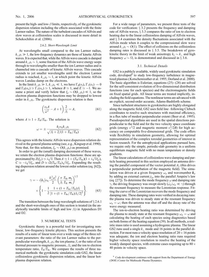
The frequency and collisionless damping rates for the threemethods are compared for temperature ratios T0i/T0e ¼ 100 and1 and for ion plasma �-values �i ¼ 10, 1, 0.1, and 0.01 over arange of k?�i from 0.1 to 100. The temperature ratio T0i/T0e ¼100 is motivated by accretion disk physics, and the tempera-ture ratio T0i/T0e ¼ 1 is appropriate for studies of the interstellarmedium and the solar wind. The real frequency ! and the damp-ing rate are normalized to the Alfven frequency kkvA. The hot-plasma calculations in this section all have kk/k? ¼ 0:001 andv thi /c ¼ 0:001. The number of Bessel functions used in the sumfor these results was 100, so the results will be accurate fork?�i P 100.

Figure 3 presents the results for the temperature ratio T0i/T0e ¼100, and Figure 4 presents those for the temperature ratioT0i/T0e ¼ 1. The results confirm accurate performance by GS2over the range of parameters tested.

3.3. Ion and Electron Heating

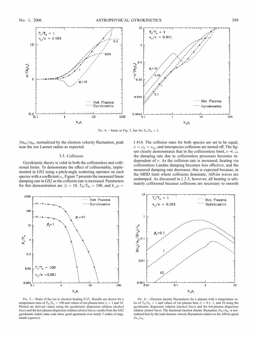
An important goal of our nonlinear gyrokinetic simulations tobe presented in future papers is to calculate the ratio of ion toelectron heating in collisionless turbulence (motivated by issuesthat arise in the physics of accretion disks; see Quataert [1998];Quataert & Gruzinov [1999]). Using the heating equation (39),the solutions of the linear collisionless dispersion relation can beused to calculate the heat deposited into the ions and electronsfor a given linear wave mode. These results for ion to electronpower are verified against estimates of the heating from the hot-plasma dispersion relation and compared to numerical resultsfromGS2 in Figure 5. The power deposited into each species Ps iscalculated by GS2 using both forms of the heating equation (39)(neglecting interspecies collisions). Here we have plotted the ionto electron power for a temperature ratio of T0i/T0e ¼ 100 and ionplasma � values of �i ¼ 1 and 10. The GS2 results agree wellwith the linear gyrokinetic and linear hot-plasma calculationsover 5 orders of magnitude in the power ratio.

3.4. Density Fluctuations

Alfven waves in the MHD limit (at large scales) are incom-pressible, with no motion along the magnetic field and no asso-ciated density fluctuations. However, asAlfvenwaves nonlinearlycascade to small scales and reach k?�i � 1, finite Larmor radiuseffects give rise to nonzero parallel motions, driving density fluc-tuations. Here we compare the density fluctuations predicted bythe linear gyrokinetic dispersion relationwith that fromhot-plasmatheory. Figure 6 compares the density fluctuations for a plasmawith temperature ratio T0i/T0e ¼ 1 and values of ion plasma �i ¼0:1, 1, and 10, parameter values relevant to the observationsof interstellar scintillation in the interstellar medium. These re-sults demonstrate that the fractional electron density fluctuations

Fig. 3.—Normalized real frequency !/kkvA (left) and damping rate /kkvA (right) vs. k?�i for a temperature ratio T0i/T0e ¼ 100 and ion plasma �-values �i ¼ 10,1, 0.1, and 0.01. Plotted are numerical solutions to the gyrokinetic dispersion relation (dashed lines), numerical solutions to the hot-plasma dispersion relation(dotted lines), and results from the GS2 gyrokinetic code (squares).


j�n0ej/n0e, normalized by the electron velocity fluctuation, peaknear the ion Larmor radius as expected.

3.5. Collisions

Gyrokinetic theory is valid in both the collisionless and colli-sional limits. To demonstrate the effect of collisionality, imple-mented in GS2 using a pitch-angle scattering operator on eachspecies with a coefficient �s, Figure 7 presents the measured lineardamping rate in GS2 as the collision rate is increased. Parametersfor this demonstration are �i ¼ 10, T0i/T0e ¼ 100, and k?�i ¼

1:414. The collision rates for both species are set to be equal,� ¼ �ii ¼ �ee, and interspecies collisions are turned off. The fig-ure clearly demonstrates that in the collisionless limit, �T!,the damping rate due to collisionless processes becomes in-dependent of �. As the collision rate is increased, heating viacollisionless Landau damping becomes less effective, and themeasured damping rate decreases; this is expected because, inthe MHD limit where collisions dominate, Alfven waves areundamped. As discussed in x 2.5, however, all heating is ulti-mately collisional because collisions are necessary to smooth

Fig. 4.—Same as Fig. 3, but for T0i/T0e ¼ 1.

Fig. 5.—Ratio of the ion to electron heating Pi/Pe. Results are shown for atemperature ratio of T0i/T0e ¼ 100 and values of ion plasma beta �i ¼ 1 and 10.Plotted are derived values using the gyrokinetic dispersion relation (dashedlines) and the hot-plasma dispersion relation (dotted lines); results from the GS2gyrokinetic initial value code show good agreement over nearly 5 orders of mag-nitude (squares).

Fig. 6.—Electron density fluctuations for a plasma with a temperature ra-tio of T0i/T0e ¼ 1 and values of ion plasma beta �i ¼ 0:1, 1, and 10 using thegyrokinetic dispersion relation (dashed lines) and the hot-plasma dispersionrelation (dotted lines). The fractional electron density fluctuation j�nej/n0e is nor-malized here by the total electron velocity fluctuations relative to the Alfven speedj�vej/vA.


out the small-scale structure in velocity space produced by wave-particle interactions. A minimum collision rate must be spec-ified for the determination of the heating rate to converge. In thelow velocity space resolution runs (10 ; 8 in velocity space) pre-sented in Figure 7, for �/ kkvA

� �< 0:01, the heating rate did not

converge accurately. Increasing the velocity-space resolution low-ers the minimum threshold on the collision rate necessary toachieve convergence.

3.6. Limits of Applicability

The gyrokinetic theory derived here is valid as long as threeimportant conditions are satisfied: (1) kkTk?, (2) !T�i , and(3) v thsTc (the nonrelativistic assumption is not essential, butit is adopted in our derivation). As discussed at the end of x 2.1,the gyrokinetic formalism retains the low-frequency dynamicsof the slow and Alfven waves and collisionless dissipation via theLandau resonance but orders out the higher frequency dynamicsof the fast MHD wave and cyclotron resonances.

A demonstration of the breakdown of the gyrokinetic approx-imation when these limits are exceeded is provided in Figure 8for a plasma with T0i/T0e ¼ 1, �i ¼ 1, and k?�i ¼ 0:1. Here, weincrease the ratio of the parallel to perpendicular wavenumberkk/k? from 0.001 to 100 and solve for the frequency using thehot-plasma dispersion relation. The frequency increases towardthe ion cyclotron frequency as the wavenumber ratio approachesunity. The frequency !/kkvA in gyrokinetics is independent ofthe value of kk, so we compare these gyrokinetic values with thehot-plasma solution. Figure 8 plots the normalized real frequency!/kkvA and damping rate j j/kkvA against the ratio of the real fre-quency to the ion cyclotron frequency !/�i. Also plotted is thevalue of kk/k? at each !/�i. At !/�i � 0:01 and kk/k? � 0:1, thedamping rate deviates from the gyrokinetic solution as cyclotrondamping becomes important. The real frequency departs fromthe gyrokinetic results at !/�i � 0:1 and kk/k? � 1. It is evidentthat gyrokinetic theory gives remarkably good results even whenkk/k? � 0:1.

4. CONCLUSION

This paper is the first in a series to study the properties of low-frequency anisotropic turbulence in collisionless astrophysicalplasmas using gyrokinetics. Our primary motivation for inves-tigating this problem is that such turbulence appears to be a nat-ural outcome of MHD turbulence as energy cascades to smallscales nearly perpendicular to the direction of the local magneticfield (see Fig. 1). Gyrokinetic turbulence may thus be a genericfeature of turbulent astrophysical plasmas.Gyrokinetics is an approximation to the full theory of colli-

sionless and collisional plasmas. The necessary assumptions arethat turbulent fluctuations are anisotropic with parallel wavenum-bers small compared to perpendicular wavenumbers, kkTk?,that frequencies are small compared to the ion cyclotron fre-quency, !T�i, and that fluctuations are small so that the typ-ical plasma or field line displacement is of order O(k�1

? ). Inthis limit, one can average over the Larmor motion of particles,simplifying the dynamics considerably. Although gyrokineticsassumes !T�i, it allows for k?�i � 1, i.e., wavelengths in thedirection perpendicular to the magnetic field can be comparableto the ion Larmor radius. On scales k?�i P 1, the gyrokinetic ap-proximation orders out the fast MHD wave but retains the slowwave and theAlfven wave.Gyrokinetics also orders out cyclotron-frequency effects such as the cyclotron resonant heating but re-tains collisionless damping via the Landau resonance.10 It is worthnoting that reconnection in the presence of a strong guide field canbe described by gyrokinetics, so the current sheets that developon scales of less than or equal to �i in a turbulent plasma are self-consistently modeled in a nonlinear gyrokinetic simulation. Theenormous value of gyrokinetics as an approximation is threefold:first, it considerably simplifies the linear and nonlinear equations;second, it removes the fast cyclotron timescales and the gyrophase

Fig. 7.—Damping rate determined in linear runs of GS2 (squares) vs. thecollision rate � normalized by kkvA. In the collisionless limit, �T!, the damp-ing rate is independent of the collision rate as expected. As the collision rate isincreased, collisionless processes for damping the wave are less effective, andthe damping rate diminishes.

Fig. 8.—For a plasma with T0i/T0e ¼ 1, �i ¼ 1, and k?�i ¼ 0:1, limits ofapplicability of the gyrokinetic solution (dashed line) as the latter deviates fromthe hot-plasma solution (dotted line) when !/�i ! 1. Also plotted (solid line) isthe value of kk/k? as a function of !/�i.

10 We are describing here the standard version of gyrokinetics. See Qin et al.(2000) for an extended theory that includes the fast-wave and high-frequencymodes.


angle dimension of the phase space; and third, it allows for asimple physical interpretation in terms of the motion of chargedrings.

In this paper, we have presented a derivation of the gyrokineticequations, including, for the first time, the equations describingparticle heating and global energy conservation. The dispersionrelation for linear collisionless gyrokinetics is derived and its phys-ical interpretation is discussed. At scales k?�iT1, the familiarMHD Alfven and slow modes are recovered. As scales such thatk?�i � 1 are approached, there is a linear mixing of the Alfvenand slowmodes. This leads to effects such as collisionless damp-ing of the Alfven wave and finite-density fluctuations in linearAlfven waves. We have compared the gyrokinetic results withthose of hot-plasma kinetic theory, showing the robustness of thegyrokinetic approximation. We also used comparisons with theanalytical results from both theories to verify and demonstratethe accuracy of the gyrokinetic simulation code GS2 in the pa-rameter regimes of astrophysical interest. We note that althoughour tests are linear, GS2 has already been used extensively for non-linear turbulence problems in the fusion research (e.g., Dorlandet al. 2000; Jenko et al. 2000, 2001; Rogers et al. 2000; Jenko &Dorland 2001, 2002; Candy et al. 2004; Ernst et al. 2004), and aprogram of nonlinear astrophysical turbulence simulations is cur-rently underway.

In conclusion, we briefly mention some of the astrophysicsproblems that will be explored in more detail in our future work:

1. Energy in Alfvenic turbulence is weakly damped until itcascades to k?�i � 1. Thus, gyrokinetics can be used to calculatethe species by species heating of plasmas by low-frequencyMHDturbulence in which the dominant heating is due to the Landauresonance. In future work, we will carry out gyrokinetic turbulentheating calculations and apply them to particle heating in solarflares, the solar wind, and hot radiatively inefficient accretionflows (see Quataert 1998; Gruzinov 1998; Quataert & Gruzinov1999; Leamon et al. 1998, 1999, 2000;Cranmer&vanBallegooijen2003, 2005, for related analytical and observational results). Theuse of the gyrokinetic formalism,which orders out high-frequencydynamics, such as fast MHD waves and cyclotron heating, isjustified on the assumption that the turbulent cascade remainshighly anisotropic down to scales of order ion Larmor radius,so that the fluctuation frequencies are well below the cyclotron

frequency even when k?�i � 1, rendering the cyclotron reso-nance unimportant to the plasma heating.

2. In situ observations of the turbulent solar wind directlymeasure the power spectra of the magnetic field (Goldstein et al.1995; Leamon et al. 1998, 1999) and the electric field (Bale et al.2005) down to scales smaller than the ion gyroradius. Thus,detailed quantitative comparisons between simulated powerspectra and the measured ones are possible. It is worth noting,however, that the solar wind is, in fact, sufficiently collisionlessthat the gyrokinetic ordering here is not entirely appropriateand the equilibrium distribution function F0 may deviate from aMaxwellian. Significant distortions of F0, however, are temperedby high-frequency kinetic mirror and firehose instabilities thatmay play the role of collisions in smoothing out the distributionfunction, so the solar wind plasma may not depart significantlyfrom gyrokinetic behavior. It must be kept inmind, however, thatif these instabilities were effective in driving a cascade to higherkk (and thus higher frequency), the gyrokinetic approximationwould be violated and further analysis required to take accountof the small-scale physics.

3. In the interstellar medium of the Milky Way, the electron-density fluctuation power spectrum, inferred from observations,is consistent with Kolmogorov turbulence over 10 decades inspatial scale (see Armstrong et al. 1995). Observations suggestthe existence of an inner scale to the density fluctuations at ap-proximately the ion Larmor radius (Spangler & Gwinn 1990).These observations may be probing the density fluctuations as-sociated with Alfven waves on gyrokinetic scales (see x 3.4)—precisely the regime that is best investigated by gyrokineticsimulations.

Much of this work was supported by the DOECenter for Mul-tiscale Plasma Dynamics, Fusion Science Center CooperativeAgreement ER54785. G. W. H. is supported by NASA grantNNG05GH78Gand byUSDOE contractDE-AC02-76CH03073.E.Q. is also supported in part byNSF grantAST 02-06006,NASAgrant NAG5-12043, an Alfred P. Sloan Fellowship, and by theDavid and Lucile Packard Foundation. A. A. S. is supported by aPPARCAdvanced Fellowship and byKing’s College, Cambridge.

APPENDIX A

DERIVATION OF THE GYROKINETIC EQUATIONS

The nonlinear gyrokinetic equation in an inhomogeneous plasma was first derived by Frieman & Chen (1982). In this appendix, wederive the nonlinear gyrokinetic equation in the simplest case in which the equilibrium is a homogeneous plasma in a constant mag-netic field, i.e.,:F0 ¼ 0 andB0 ¼ B0 z in a periodic box.We begin with the Fokker-Planck equation andMaxwell’s equations. The gyro-kinetic ordering, which makes the expansion procedure possible, was explained in x 2.1. The guiding center coordinates and the keymathematical operation, ring averaging, were introduced in x 2.3. In what follows, the Fokker-Planck equation is systematically expandedunder the gyrokinetic ordering. Theminus first, zeroth, and first orders are solved to determine both the formof the equilibriumdistributionfunction and the evolution equation for the perturbed distribution function, the gyrokinetic equation (the slow evolution of the equilibriumenters in the second order and is worked out in Appendix B). At each order, a ring average at constant guiding center position is employedto eliminate higher orders from the equation. Velocity integration of the perturbed distribution function yields the charge and currentdensities that appear in the gyrokinetic versions of Maxwell’s equations.

A1. MAXWELL’S EQUATIONS AND POTENTIALS

Let us start with Poisson’s law. The equilibrium plasma is neutral,P

s qsn0s ¼ 0, so we have

: = �E ¼ 4�Xs

qs�ns: ðA1Þ


The left-hand side is O(�B0v thi /c�i) (see eq. [8]), and the right-hand side is O(�qin0i), so the ratio of the divergence of the electricfield to the charge density is O(��1

i v 2thi /c2). Therefore, in the limit of nonrelativistic ions, the perturbed charge density is zero.11 This

establishes the condition of quasineutrality: Xs

qs�ns ¼ 0: ðA2Þ

In Faraday’s law,

c: < �E ¼ � @�B

@t; ðA3Þ

the left-hand side is O(��i B0), whereas the right-hand side is O(�2�iB0). Therefore, to dominant order the electric field satisfies: < �E ¼ 0, so the largest part of the electric field is electrostatic. The inductive electric field does, however, gives an importantcontribution to the parallel electric field. The electric and magnetic fields are most conveniently written in terms of the scalar potential� and vector potential A:

�E ¼ �:�� 1

c

@A

@t; �B ¼ : < A: ðA4Þ

We choose the Coulomb gauge : = A ¼ 0. Thus, with the gyrokinetic ordering, to O(�2), the vector potential is

A ¼ Akzþ A? ¼ Akzþ:k < z: ðA5Þ

Hence, the perturbed magnetic field to O(�2) is given by

�B ¼ :Ak < z�:2k z ¼ :Ak < zþ �Bkz: ðA6Þ

We use the scalars Ak and �Bk (rather than k) in subsequent development.Consider next the Ampere-Maxwell law:

: < �B ¼ 4�

c� jþ 1

c

@�E

@t: ðA7Þ

The left-hand side isO(�B0�i/v thi ), while the second term in the left-hand side (the displacement current) isO(� 2B0�iv thi /c2). The ratio of

the latter to the former is, therefore,O(�v2thi /c2), so we can drop the displacement current and use the pre-Maxwell form of Ampere’s law:

: < �B ¼ �:2A ¼ �: 2Akzþ:�Bk < z ¼ 4�

c� j: ðA8Þ

A2. THE GYROKINETIC EQUATION

Let us start with the Fokker-Planck equation

dfs

dt¼ @fs

@tþ v =:fs þ

qs

ms

�:�� 1

c

@A

@tþ v < B

c

� �=@fs@v

¼ @fs@t

� �coll

¼ Csr( fs; fr)þ Css( fs; fs); ðA9Þ

where the right-hand side is the standard Fokker-Planck integrodifferential collision operator (e.g., Helander & Sigmar 2002). Theexpression Csr( fs; fr) denotes the effect of collisions of species s on (the other) species r, and Css( fs; fs) denotes like-particle colli-sions. To reduce the clutter, we suppress the species label s in this section and denote the entire collision term by C( f ; f ).

The distribution function is expanded in powers of �:

f ¼ F0 þ �f ; �f ¼ �f1 þ �f2 þ : : : ; ðA10Þ

where �fn � O(� nF0). With the ordering defined by equations (8)–(13), the terms in the Fokker-Planck are ordered as follows:

@F0=@t þ@�f =@t þv? =:�f þvkz =:�f

�2 � 1 �

þ q

mc�c:�ð Þ �@A=@t þv < �B þ v < B0ð Þ = @F0=@v

1 � 1 1=�

þ q

mc�c:�ð Þ �@A=@t þv < �B þ v < B0ð Þ = @�f=@v

� �2 � 1

¼C(F0;F0) þC(�f ;F0) þC(F0; �f ) þC(�f ; �f );

1 � � �2

ðA11Þ

11 Alternatively, one can say that the divergence of the electric field is small for gyrokinetic perturbations whose wavelengths are long compared to the electronDebye length, kDe .


where we label below each term its order relative to F0v thi /l0. We now proceed with the formal expansion.

A2.1. Minus First Order, O(1/�)

From equation (A11), in velocity variables transformed from v to (v, v?, � ), we obtain at this order

@F0

@�¼ 0; ðA12Þ

so the equilibrium distribution function does not depend on gyrophase angle, F0 ¼ F0(v; v?; t).

A2.2. Zeroth Order, O(1)

At this order, equation (A11) becomes

v? =:�f1 þq

m�:�þ v < �B

c

� �=@F0

@v� �

@�f1@�

¼ C(F0;F0): ðA13Þ

At this stage both F0 and �f1 are unknown. To eliminate �f1 from this equation (and thereby isolate information about F0), we multiplyequation (A13) by 1þ ln F0 and integrate over all space and all velocities, making use of equation (A12) and assuming that perturbedquantities spatially average to zero (this is exactly true in a periodic box). We findZ

d 3r

Zd 3v ( ln F0)C(F0;F0) ¼ 0: ðA14Þ

It is known from the proof of Boltzmann’s H-theorem that this uniquely constrains F0 to be a Maxwellian:

F0 ¼n0

�3=2v3thexp � v2

v 2th

� �; ðA15Þ

where the mean plasma flow is assumed to be zero. The temperature T0(t) ¼ (1/2)mv2th associated with this Maxwellian varies on theslow (heating) timescale, theat � O(��2l0/v th), due to conversion of the turbulent energy into heat. In Appendix B, we determine thisheating in the second order of the gyrokinetic expansion. The density n0 does not vary because the number of particles is conserved. Inmost other derivations of gyrokinetics, F0 is not determined, although it is often assumed to be a Maxwellian.

Substituting the solution for F0 (eq. [A15]) into equation (A13) and using C(F0;F0) ¼ 0 yields

v? =:�f1 � �@�f1@�

¼ �v =:q�

T0

� �F0: ðA16Þ

This inhomogeneous equation for �f1 supports a particular solution and a homogeneous solution. Noting the particular solution �fp ¼�(q�/T0)F0 þ O(�2F0), the first-order perturbation is written as �f1 ¼ �(q�/T0)F0 þ h, where the homogeneous solution h satisfies

v? =:h� �@h

@�

� �r

¼ @h

@�

� �R

¼ 0; ðA17Þ

where we have transformed the � derivative at constant position r to one at constant guiding center R. Thus, h is independent of thegyrophase angle at constant guiding center R (but not at constant position r): h ¼ h(R; v; v?; t). Therefore, the complete solution forthe distribution function, after taking 1� q�/T0 ¼ exp (�q�/T0)þ O(� 2) and absorbing O(�2) terms into �f2, is

f ¼ F0(v; �2t) exp � q�(r; t)

T0

� �þ h(R; v; v?; t)þ �f2 þ : : : ðA18Þ

The first term in the solution is the equilibrium distribution function corrected by the Boltzmann factor. Physically this arises from therapid (compared to the evolution of �) motion of electrons along and ions across the field lines attempting to set up a thermal equilibriumdistribution. However, the motion of the particles across the field is constrained by the gyration, and the particles are not (entirely) free toset up thermal equilibrium. The second term is the gyrokinetic distribution function that represents the response of the rings to the per-turbed fields.

A2.3. First Order, O(�)

Plugging in the form of solution given in equation (A18) and transforming into guiding-center spatial coordinates and velocitycoordinates (v, v?, � ), the Fokker-Planck equation to this order becomes

@h

@tþ dR

dt=@h

@Rþ q

m�:?�þ v < �B

c

� �=

v

v

@h

@vþ v?

v?

@h

@v?

� �� C(h;F0)� C(F0; h) ¼ �

@�f2@�

� �R

þ q

T0

@�

@t� v

c=@A

@t

� �F0; ðA19Þ


where

dR

dt¼ vkzþ

c

B0

�:�� 1

c

@A

@tþ v < �B

c

� �< z: ðA20Þ

Note that the linearized collision operator C(h;F0)þ C(F0; h) involves h and F0 both of electrons and of ions.To eliminate �f2 from equation (A19), we ring average the equation over � at fixed guiding centerR, taking advantage of the fact that

�f2 must be periodic in �. The ring averaging also eliminates the third term on the left-hand side. Indeed, for an arbitrary function a(r),

v? = :ah iR ¼ �� v < zð Þ = @

@v

v < z

�

� �= :a

� �R

¼ � v < zð Þ = @r

@v

� �R

= :a

� �R

¼ � v < zð Þ = @a

@v

� �R

� �R

¼ ��@a

@�

� �R

� �R

¼ 0;

ðA21Þ

from which hv = :?�iR ¼ 0 and hv? = (v < �B)iR ¼ vkhv? = (z < �B)iR ¼ vkhv? = :?AkiR ¼ 0 (see eq. [A6]). Thus, the ring-averagedequation (A19) takes the form

@h

@tþ dR

dt

� �R

=@h

@R� @h

@t

� �coll

¼ q

T0

@hiR@t

F0; ðA22Þ

where we have defined the gyrokinetic collision operator (@h/@t)coll ¼ hC(h;F0)þ C(F0; h)iR and the gyrokinetic potential ¼�� v = A/c. Keeping only first-order contributions in equation (A20) and substituting for �B from equation (A6), we find that the ring-averaged guiding center motion is given by

dR

dt

� �R

¼ vkz�c

B0

:?�h iR < zþvkB0

:?Ak �

R< z� 1

B0

v?�Bk �

R¼ vkz�

c

B0

@hiR@R

< z; ðA23Þ

where we have used the identity v?�Bk �

R¼ � :?(v? = A?)h iR. Substituting equation (A23) into equation (A22), we obtain the

gyrokinetic equation:

@h

@tþ vkz =

@h

@Rþ c

B0

hiR; h½ � � @h

@t

� �coll

¼ q

T0

@hiR@t

F0; ðA24Þ

where the nonlinear effects enter via the Poisson bracket, defined by

hiR; h½ � ¼ @hiR@R

< z

� �=@h

@R¼ @hiR

@X

@h

@Y� @hiR

@Y

@h

@X: ðA25Þ

The gyrokinetic equation (A24) describes the time evolution of h, the ring distribution function. The second term on the left-hand sidecorresponds to the ring motion along B0, the third term to the ring motion across B0, and the fourth term to the effect of collisions. Thesource term on the right-hand side is the ring-averaged change in the energy of the particles. A more detailed discussion of the physicalaspects of this equation is given in x 2.4. The equilibrium distribution functionF0 changes only on the slow (heating) timescale and is thusformally fixed (stationary) with respect to the timescale of equation (A24). The evolution of F0 is calculated in Appendix B.

A3. THE GYROKINETIC FORM OF MAXWELL’S EQUATIONS

To complete the set of gyrokinetic equations, we need to determine the electromagnetic field, which is encoded by . To determinethe three unknown scalars �,Ak, and �Bk (which relates toA? via eqs. [A4] and [A6]), we use the quasineutrality condition, equation (A2),and Ampere’s law, equation (A8), taken at O(�) in the gyrokinetic ordering.

A3.1. The Quasineutrality Condition

The charge density needed in the quasineutrality condition, equation (A2), can be determined by multiplying the distributionfunction, equation (A18), expanded to first order O(�), by the charge qs and integrating over velocities. Expanding the exponential inthe Boltzmann term and dropping terms of order O(�2) and higher gives

Xs

� q2s n0s

T0s�þ qs

Zd 3v hs rþ v < z

�s

; v; t

� �� ¼ 0: ðA26Þ

Note that the velocity integral must be performed at a fixed position r, because the charge must be determined at a fixed position r, not at afixed guiding center R. Using the ring average at constant r (eq. [22]), the quasineutrality condition can be written in the following form

Xs

� q2s n0s

T0s�þ qs

Zd 3v hhsir

� �¼ 0: ðA27Þ


A3.2. The Parallel Ampere’s Law

The current density is calculated by multiplying the distribution function, equation (A18), expanded to first order O(�), by qsv andintegrating over velocities. The Boltzmann part of the current is odd with respect to vk and vanishes on integration. The parallelcomponent of Ampere’s law, equation (A8), is, therefore,

�:2?Ak ¼

4�

c�jk ¼

Xs

4�

cqs

Zd 3v vkhhsir; ðA28Þ

where the ring average at a fixed position r appears in the same fashion as in equation (A27).

A3.3. The Perpendicular Ampere’s Law

The perpendicular component of Ampere’s law, equation (A8), is derived in an analogous manner as the parallel component inAppendix A.3.2: Ampere’s law is crossed with z, the Boltzmann contribution vanishes on integration over gyrophase angle �, and aring average at a fixed position r is performed. The result is

:?�Bk ¼4�

cz < � j ¼

Xs

4�

cqs

Zd 3v h z < v?hsir: ðA29Þ

It is straightforward to show that equation (A29) is the gyrokinetic version of perpendicular pressure balance (no fast magnetosonicwaves). Integration by parts yields

:?B0�Bk4�

¼ �:? = �P?; ðA30Þ

where the perpendicular pressure tensor is

�P? ¼Xs

ms

Zd 3v v?v?hsh ir: ðA31Þ

In order to drive steady state (nondecaying) turbulence, we introduce an additional externally driven antenna current ja to the right-hand sides of equations (A28) and (A29).

APPENDIX B

DERIVATION OF THE HEATING EQUATION

While the gyrokinetic equation (A24) determines the evolution of the perturbation to the distribution function on the intermediatetimescale, we must go to second order, O(�2!), in the gyrokinetic ordering to obtain the slow evolution of the equilibrium distributionfunctionF0. This appendix contains two derivations of the heating equation (39): the first ismore conventional, but longer (Appendix B.1);the second employs entropy conservation and is, in a sense, more intuitive and fundamental (Appendix B.2). We also discuss energy con-servation in driven systems and derive the power balance equation (40) (see Appendix B.3).

B1. CONVENTIONAL DERIVATION OF THE HEATING EQUATION

We begin by defining the medium-time average over a period�t long compared to the fluctuation timescale but short compared tothe heating timescale, 1/!T�tT1/�2!,

a(t) ¼ 1

�t

Z tþ�t=2

t��t=2

dt 0 a(t 0): ðB1Þ

The equilibrium distribution function F0 is constant at times ��t, so F0 ¼ F0.To determine the evolution of the equilibrium density and temperature of a species s on the heating (transport) timescale, we consider the

full (not ring-averaged) Fokker-Planck equation (A9). To demonstrate that particle conservation implies that n0s is a constant, we integrateequation (A9) over all space and velocity, divide by system volume V, and discard all terms of order O(�3) and higher:Z

d 3r

V

Zd 3v

@fs@t

¼ dn0s

dtþ d

dt

Zd 3r

V

Zd 3v �f2s ¼ 0: ðB2Þ

Herewe have used the conservation of particles by the collision operator, the fact that the first-order perturbations spatially average to zero,and an integration by parts over velocity to simplify the result. Performing the medium-time average (eq. [B1]) eliminates the �f2s term,leaving

dn0s

dt¼ 0: ðB3Þ

Thus, for both species s, the density n0s is constant on the heating (transport) timescale.


The evolution of the temperature T0s is calculated similarly by multiplying equation (A9) by msv2/2, integrating over all space and

velocity, and dividing by the system volumeV. Using the expansion of the distribution function, integration by parts in velocity, we get

3

2n0s

dT0s

dtþ d

dt

Zd 3r

V

Zd 3v

msv2

2�f2s ¼

Zd 3r

V

Zd 3v qs(v = E ) fs þ

Zd 3r

V

Zd 3v

msv2

2Csr( fs; fr): ðB4Þ

We have again assumedRd 3r �f1s ¼ 0 (first-order perturbations spatially average to zero). The first term on the right-hand side is the

work done on the particles by the fields, and the second is the collisional energy exchange between species. Note that collisionsbetween like particles do not produce a net loss of energy for a species and thus do not appear in this expression (the operator Css

integrates to zero). At this order, the collisions between species occur only between the Maxwellian equilibria of each interactingspecies; the standard form of this collisional energy exchange (see, e.g., Helander & Sigmar 2002) is given byZ

d 3r

V

Zd 3v

msv2

2Csr( fs; fr) ¼ n0s�

srE (T0r � T0s): ðB5Þ

Expressions for the interspecies collision rate � srE can be found in Helander & Sigmar (2002). The collisional energy exchange rate of

ions on electrons, � ieE , is a factor (me/mi)

1/2 times smaller than the ion-ion collision rate. It is, therefore, possible to sustain a tem-perature difference between ions and electrons even though the plasma is collisional enough to make F0 Maxwellian for each species.

Splitting the electric field into potentials, E ¼ �:�� (1/c)@A/@t, we can manipulate the scalar potential part into a more usefulhigher order form. After some algebra and using equation (B5), we find

3

2n0s

dT0s

dtþ d

dt

Zd 3r

V

Zd 3v

msv2

2�f2s þ qs��fs

� �¼Z

d 3r

V

Zd 3v qs

@

@t�� v = A

c

� ��fs þ n0s�

srE (T0r � T0s); ðB6Þ

where �fs is the entire perturbed part of the distribution function. From this equation, we can check the order of the heating rate,

3

2n0s

dT0s

dt� O(�2!T0s): ðB7Þ

We see that the variation in the equilibrium quantities is, as expected, on a timescale that is �2 slower than the timescale of the vari-ations in the fluctuating quantities. Note that this ordering is consistent with all the energy in an Alfven wave cascade becoming heat ina single cascade time at the driving scale.

Splitting the perturbed distribution function �fs into the Boltzmann and gyrokinetic parts (eq. [A18]), we obtain the followinginstantaneous form of the heating equation

3

2n0s

dT0s

dtþ d

dt

Zd 3r

V

Zd 3v

msv2

2�f2s þ qs�hs

� ��Z

d 3r

V

n0sq2s�

2

2T0s

� �¼Z

d 3r

V

Zd 3v qs

@

@ths þ n0s�

srE (T0r � T0s): ðB8Þ

To obtain the heating equation (39), we take the medium-time average, defined by equation (B1), of the above equation. The averageof the second term on the left-hand side is zero; it does not contribute to the average heating. Thus, we do not require the second-orderperturbed distribution function �f2s to calculate the heating. The average of the first term on the right-hand side of equation (B8) is thedesired heating term that relates the slow-timescale evolution of the equilibrium to the solution of the gyrokinetic equation. The rintegral is converted into theRs integral by noticing that

Rd 3r

Rd 3v ¼

Rd 3v

Rd 3Rs (the velocity integration on the left is at constant

r, while on the right it is at constant Rs). Therefore,Zd 3r

V

Zd 3v qs

@(r)

@ths(Rs) ¼

Zd 3v

Zd 3Rs

Vqs

@

@t Rs �

v < z

�s

� �� hs(Rs) ¼

Zd 3v

Zd 3Rs

Vqs

@hiRs

@ths: ðB9Þ

We must now demonstrate that the heating is ultimately collisional (the second equality in eq. [39]). To make this connection, wemultiply the gyrokinetic equation (A24) by T0shs/F0s and integrate over space (i.e., with respect to Rs) and velocity to obtain thefollowing equation

d

dt

Zd 3v

Zd 3Rs

V

T0s

2F0s

h2s �Z

d 3v

Zd 3Rs

V

T0s

F0s

hs@hs@t

� �coll

¼Z

d 3v

Zd 3Rs

Vqs

@hiRs

@ths ðB10Þ

(for reasons that become apparent in Appendix B.2, this is referred to as the entropy-balance equation). Combining equations (B8) and(B10) using equation (B9) then gives the collisional form of the instantaneous heating equation:

3

2n0s

dT0s

dtþ d

dt

Zd 3r

V

Zd 3v

msv2

2�f2s þ qs�hhsir �

T0s

2F0s

hh2s ir� �

�Z

d 3r

V

n0sq2s �

2

2T0s

� �

¼�Z

d 3r

V

Zd 3v

T0s

F0s

hs@hs@t

� �coll

� �r

þ n0s�srE (T0r � T0s); ðB11Þ


where we have usedRd 3r

Rd 3v a(Rs) ¼

Rd 3r

Rd 3v hair (this manipulation is done purely for notational cleanliness: the expressions

under the integrals are now explicitly functions of r and v, not of Rs). Under medium-time averaging, the second term on the left-handside of equation (B11) again vanishes, and the second equality in equation (39) is obtained:

3

2n0s

dT0s

dt¼ �

Zd 3r

V

Zd 3v

T0s

F0s

hs@hs@t

� �coll

� �r

þ n0s�srE (T0r � T0s): ðB12Þ

The term that has averaged out does not contribute to the net (slow-timescale) heating because it represents the sloshing of energyback and forth between particles and fields (on the fluctuation timescale). On the right-hand side, the collisional term is negative def-inite for like-particle and pitch-angle collision operators. [These are the only relevant cases: for s ¼ i, the ion-ion collisions dominate,and for s ¼ e, the dominant terms are electron-electron collisions and the pitch-angle scattering of the electrons off the ions; all otherparts of the collision operator are subdominant by at least one factor of (me/mi)

1/2.]The equation (B12) for the heating on the slow timescale is sign-definite, so it is, in practice, easier to average numerically than the

instantaneous heating equation (B8): unlike in equation (B8), calculating the average heating does not require precisely capturing theeffect of near-cancellation of the intermediate-timescale oscillations of the instantaneous energy transfer between particles and waves.The net heating is always collisional, regardless of the collision rate—when collisions are small, hs develops small scales in velocityspace, typically�v � O(�1/2), so that the heating is independent of the collision rate �. As we shall see below, equation (B12) relatesheating to the collisional entropy production.

B2. ENTROPY ARGUMENT TO DERIVE THE HEATING EQUATION

Ignoring the ion-electron collisions, whose rate is (me/mi)1/2 times smaller than that of the ion-ion collisions, Boltzmann’sH-theorem

gives the time evolution of the entropy of the ions Si as follows:

dSi

dt¼ � d

dt

Zd 3r

V

Zd 3v fi ln fi ¼ �

Zd 3r

V

Zd 3 v ln fiCii( fi; fi): ðB13Þ

It can be easily shown that the right-hand side is nonnegative (see, e.g., Lifshitz & Pitaevskii 1981) and, therefore, that entropy alwaysincreases. It can also be shown that the entropy increase is zero if, and only if, the distribution function is a Maxwellian. Expandingfi about the Maxwellian F0i , we obtain, to order O(� 2),

dSi

dt¼ � d

dt

Zd 3r

V

Zd 3v F0i ln F0i þ (1þ ln F0i)�f2i þ

�f 21i2F0i

� �¼ �

Zd 3r

V

Zd 3v

�f1iF0i

@�f1i@t

� �coll

; ðB14Þ

where we have made use of the energy conservation properties of ion-ion collisions and of the fact that �f1i spatially averages to zero.Evaluating the zeroth-order (Maxwellian) part of the integral on the left-hand side and splitting �f1i into the Boltzmann and gyro-kinetic parts (eq. [A18]), we obtain the slow evolution of temperature

3

2n0i

1

T0i

dT0i

dtþ d

dt

Zd 3r

V

Zd 3v

miv2

2T0i�f2i þ

qi�

T0ihi �

h2i2F0i

� ��Z

d 3r

V

n0iq2i �

2

2T 20i

� �¼ �

Zd 3r

V

Zd 3v

1

F0i

hi@hi@t

� �coll

� �r

: ðB15Þ

This result is the same as equation (B11); the heating is now manifestly expressed as the irreversible entropy production. Undermedium-time average, the second term on the left-hand side of equation again vanishes, so the heating equation (B12) is recovered.

B3. ENERGY CONSERVATION IN DRIVEN SYSTEMS

To determine an equation for the conservation of energy in gyrokinetics, we use Poynting’s theorem

d

dt

Zd 3r

E 2

8�þ B2

8�

� �þ c

4�

IdS = (E < B) ¼ �

Zd 3r jþ jað Þ = E; ðB16Þ

where ja is the current in the antenna driving the system and j is the plasma current. We shall drop the surface term (the Poynting flux)—this is justified, e.g., in a numerical box with periodic boundary conditions.

From x 2.1, we know that j�Ej2 � O(� 2B20v2thi /c

2) and j�Bj2� O(�2B20) (eq. [8]). Thus, in the nonrelativistic limit, the magnetic

energy dominates, and we may neglect the electric field energy (this is consistent with neglecting the displacement current in thenonrelativistic ordering). We are left with

d

dt

Zd 3r

j�Bj2

8�¼ �

Zd 3r jþ jað Þ = E: ðB17Þ

Under medium-time averaging, the left-hand side vanishes, and we are left with the steady state balance:Zd 3r jþ jað Þ = E ¼ 0: ðB18Þ


On the other hand, using equations (B4) and (B11) to calculateRd 3r ( j = E ) ¼

Rd 3r

Ps

Rd 3v qs(v = E ) fs, we can convert equa-

tion (B17) into the following instantaneous power-balance equation

d

dt

Zd 3r

V

Xs

Zd 3v

T0s

2F0s

hs �qs�

T0sF0s

� �2þ j�Bj2

8�

" #¼Xs

Zd 3r

V

Zd 3v

T0s

F0s

hs@hs@t

� �coll

� �r

�Z

d 3r

Vja = E: ðB19Þ

The first term on the right-hand side is the nonnegative-definite collisional entropy production (see eq. [B15]); the second term is theexternal energy input. The left-hand side is the time derivative of the fluctuation energy (kinetic plus magnetic):

�W ¼Z

d 3r

V

Xs

Zd 3v

T0s�f2s

2F0s

þ j�Bj2

8�

" #: ðB20Þ

Note that in the large-scale limit, appropriate for MHD, we have Alfven waves, for which hs ’ qs �h iRs/T0s—the kinetic energy then

becomes the E < B velocity squared as it should be in MHD.If we medium-time average equation (B19), the left-hand side vanishes, and we have the power balance between external energy

injection and collisional dissipation:

Xs

Zd 3r

V

Zd 3v

T0s

F0s

hs@hs@t

� �coll

� �r

¼Z

d 3r

Vja = E: ðB21Þ

APPENDIX C

DERIVATION OF THE LINEAR COLLISIONLESS DISPERSION RELATION

The dispersion relation for a linear, collisionless gyrokinetic system is derived beginning with the linearized collisionless version ofthe gyrokinetic equation (25),

@hs@t

þ vk@hs@z

¼ qs

T0sF0s

@hiRs

@t; ðC1Þ

and the field equations (A27)–(A29). First, the electromagnetic fields and the gyrokinetic distribution function are expanded in planewaves, allowing the ring averages appearing in the equations to be written as multiplications by Bessel functions. The gyrokineticequation is then solved algebraically for the distribution function. Next, this solution is substituted into equations (A27)–(A29), andthe integration over velocity is performed using the plasma dispersion function to simplify the parallel velocity integrals and modifiedBessel functions to express the perpendicular velocity integrals. The condition for the existence of a solution to the resulting set ofalgebraic equations is the dispersion relation. In this appendix, the plasma species subscript s is suppressed when unnecessary.

C1. SOLVING FOR THE DISTRIBUTION FUNCTION

First, we decompose the electromagnetic potentials into plane wave solutions of the form a(r; t) ¼ a exp ½i(k = r� !t)� (where adenotes , �, or A) and the gyrokinetic distribution function into solutions of the form h(R; v; v?; t) ¼ h exp ½i(k = R� !t)�. To solveequation (C1) for h, we need to express hiR in algebraic terms. Under the plane wave decomposition, ring averages reduce tomultiplications by Bessel functions. For example, the terms with the scalar potential � in the definition of ¼ �� v = A /c yield

h�(r; t)iR ¼ �e i(k = R�!t) 1

2�

Id� exp i

k?v?�

cos �

� �¼ J0

k?v?�

� ��e i(k = R�!t): ðC2Þ

Here we have used the definition of the zeroth-order Bessel function (Abramowitz & Stegun 1972) and the relation between theposition and guiding center, equation (19), noting that k = z < v/�ð Þ ¼ (k?v?/�) cos �, where � is the angle between k? and the par-ticle’s instantaneous Larmor radius z < v/�. After further algebraic manipulations of this kind, the ring-averaged potential hiR can bewritten in terms of zeroth- and first-order Bessel functions,

hiR ¼ J0k?v?�

� ��

vk Akc

!þ J1 k?v?=�ð Þ

k?v?=�

mv2?q

�BkB0

" #e i(k = R�!t); ðC3Þ

where we have used the definition �Bk ¼ i(k? < A?) = z. Similarly, the ring average of the distribution function at constant r becomes

hh(R; v; v?; t)ir ¼ J0k?v?�

� �he i(k = r�!t): ðC4Þ


The linearized gyrokinetic equation can now be solved for the distribution function:

h ¼ qF0

T0

!

!� kkvkhiR: ðC5Þ

Using equation (C3), this can be written in terms of the potentials as follows:

h ¼ qF0

T0J0

k?v?�

� �!A kkkc

þ !

!� kkvkJ0

k?v?�

� ��

!A kkkc

!þ J1 k?v?=�ð Þ

k?v?=�

2v 2?v2th

T0

q

�BkB0

" #( ): ðC6Þ

C2. PERFORMING THE INTEGRATION OVER VELOCITY

Because the solution for the distribution function, equation (C6), is a product of functions of vk and v?, the integrals over velocityspace,

Rd 3v ¼

R 1�1 dvk

R 10

v? dv?R 2�0

d�, in equations (A27)–(A29) can be expressed in terms of plasma dispersion functions andmodified Bessel functions.

Integrals over vk, when not immediately completed, are written in terms of the plasma dispersion function (Fried & Conte 1961)

Z(� ) ¼ 1ffiffiffi�

pZL

dxe�x 2

x� �; ðC7Þ

where � ¼ !/ kk v th and the integral is performed over the Landau contour from �1 to +1 below the pole at x ¼ � in the complex

plane. Using this definition, we can write

1ffiffiffi�

pZ

dvkv th

e�v 2k =v

2th

!

!� kkvk¼ ��Z(� ): ðC8Þ

Integrations over v? can be written in terms of modified Bessel functions. Three such integrals arise:

�0(�) ¼Z 1

0

2v? dv?v2th

J0k?v?�

� �� 2e�v 2?=v

2th ¼ I0(�)e

��;

�1(�) ¼Z 1

0

2v? dv?v2th

2v2?v 2th

J0 k?v?=�ð ÞJ1 k?v?=�ð Þk?v?=�

e�v 2?=v2th ¼ ½I0(�)� I1(�)�e��;

�2(�) ¼Z 1

0

2v? dv?v2th

4v4?v4th

J1 k?v?=�ð Þk?v?=�

� �2e�v 2?=v

2th ¼ 2�1(�); ðC9Þ

where I0 and I1 are the modified Bessel functions, � ¼ k 2?�

2/2, and we have used the relation (Watson 1966),Z 1

0

dx xJn( px)Jn(qx)e�a2x2 ¼ 1

2a2In

pq

2a2

� �e�( p

2þq2)=4a2

: ðC10Þ

C3. QUASINEUTRALITY CONDITION

Beginning with the gyrokinetic quasineutrality condition, equation (A27), we write the ring average of the distribution function atconstant position r as a multiplication by a Bessel function (eq. [C4]) and substitute h from equation (C6) into the velocity integral.This gives

Xs

q2s n0s

T0s� ¼

Xs

2�qs

Z 1

�1dvk

Z 1

0

v? dv? J0k?v?�s

� �hs

¼Xs

q2s n0s

T0s�0(�s)

!A kkkc

� �0(�s)�sZ(�s) ��!A kkkc

!� �1(�s)�sZ(�s)

T0s

qs

�BkB0

" #; ðC11Þ

where, in performing the velocity integrals, we have used the definitions given in x C2.

C4. PARALLEL AMPERE’S LAW

Following a similar sequence of steps for the parallel Ampere’s law, equation (A28), we have

k 2?Ak ¼

4�

c

Xs

2�qs

Z 1

�1dvk

Z 1

0

v? dv? J0k?v?�s

� �vkhs

¼� 4�!

ckk

Xs

q2s n0s

T0s1þ � s Z(�s)½ � �0(�s) ��

!A kkkc

!þ �1(�s)

T0s

qs

�BkB0

" #: ðC12Þ


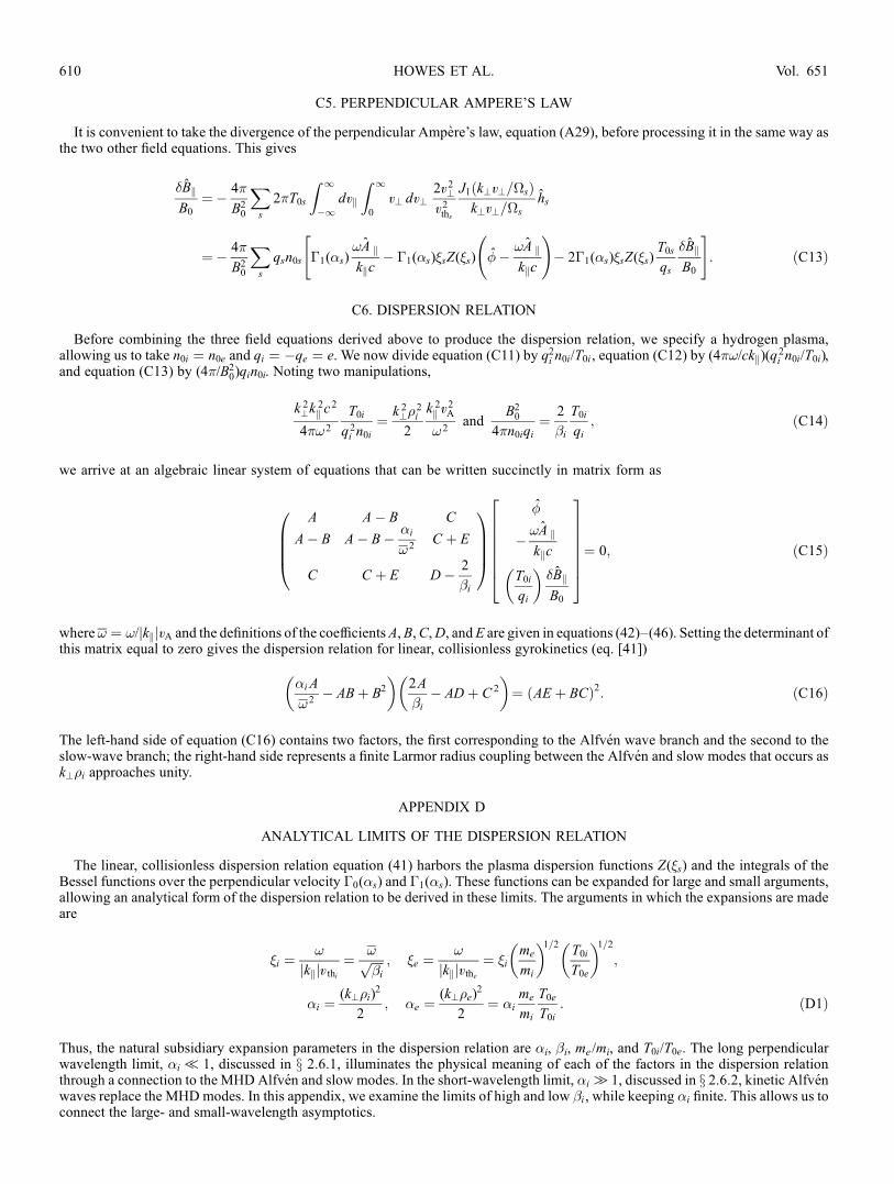
C5. PERPENDICULAR AMPERE’S LAW

It is convenient to take the divergence of the perpendicular Ampere’s law, equation (A29), before processing it in the same way asthe two other field equations. This gives

�BkB0

¼� 4�

B20

Xs

2�T0s

Z 1

�1dvk

Z 1

0

v? dv?2v2?v2ths

J1 k?v?=�sð Þk?v?=�s

hs

¼� 4�

B20

Xs

qsn0s �1(�s)!A kkkc

� �1(�s)�sZ(�s) ��!A kkkc

!� 2�1(�s)�sZ(�s)

T0s

qs

�BkB0

" #: ðC13Þ

C6. DISPERSION RELATION

Before combining the three field equations derived above to produce the dispersion relation, we specify a hydrogen plasma,allowing us to take n0i ¼ n0e and qi ¼ �qe ¼ e. We now divide equation (C11) by q2i n0i/T0i , equation (C12) by (4�!/ckk)(q

2i n0i/T0i),

and equation (C13) by (4�/B20)qin0i. Noting two manipulations,

k 2?k

2k c

2

4�!2

T0i

q2i n0i

¼ k 2?�

2i

2

k 2k v

2A

!2and

B20

4�n0iqi¼ 2

�i

T0i

qi; ðC14Þ

we arrive at an algebraic linear system of equations that can be written succinctly in matrix form as

A A� B C

A� B A� B� �i

!2C þ E

C C þ E D� 2

�i

0BBB@

1CCCA

�

�!A kkkc

T0i

qi

� ��BkB0

26666664

37777775¼ 0; ðC15Þ

where! ¼ !/jkkjvA and the definitions of the coefficientsA,B,C,D, andE are given in equations (42)–(46). Setting the determinant ofthis matrix equal to zero gives the dispersion relation for linear, collisionless gyrokinetics (eq. [41])

�i A

!2� ABþ B2

� �2A

�i

� AD þ C 2

� �¼ AE þ BCð Þ2: ðC16Þ

The left-hand side of equation (C16) contains two factors, the first corresponding to the Alfven wave branch and the second to theslow-wave branch; the right-hand side represents a finite Larmor radius coupling between the Alfven and slow modes that occurs ask?�i approaches unity.

APPENDIX D

ANALYTICAL LIMITS OF THE DISPERSION RELATION

The linear, collisionless dispersion relation equation (41) harbors the plasma dispersion functions Z(�s) and the integrals of theBessel functions over the perpendicular velocity �0(�s) and �1(�s). These functions can be expanded for large and small arguments,allowing an analytical form of the dispersion relation to be derived in these limits. The arguments in which the expansions are madeare

�i ¼!

jkkjv thi¼ !ffiffiffiffi

�i

p ; �e ¼!

jkkjvthe¼ �i

me

mi

� �1=2T0i

T0e

� �1=2;

�i ¼(k?�i)

2

2; �e ¼

(k?�e)2

2¼ �i

me

mi

T0e

T0i: ðD1Þ

Thus, the natural subsidiary expansion parameters in the dispersion relation are �i, �i, me /mi, and T0i/T0e. The long perpendicularwavelength limit, �iT1, discussed in x 2.6.1, illuminates the physical meaning of each of the factors in the dispersion relationthrough a connection to the MHD Alfven and slow modes. In the short-wavelength limit, �i 31, discussed in x 2.6.2, kinetic Alfvenwaves replace the MHDmodes. In this appendix, we examine the limits of high and low �i , while keeping �i finite. This allows us toconnect the large- and small-wavelength asymptotics.


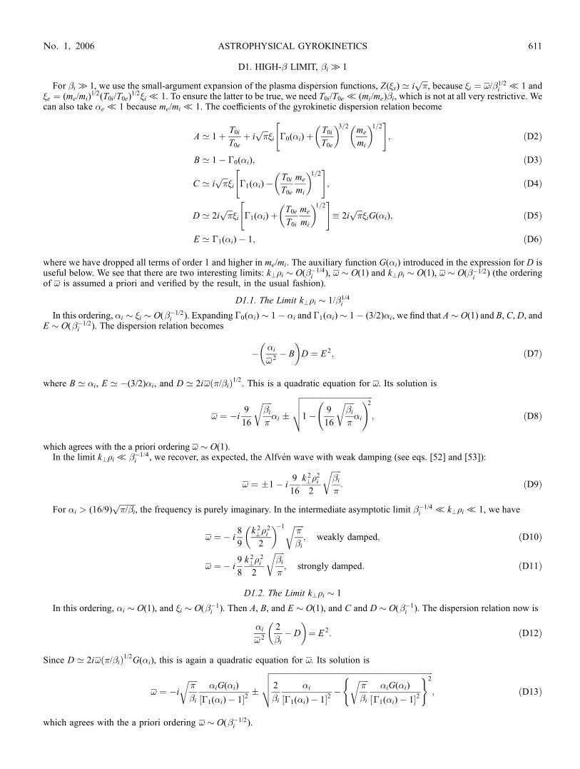
D1. HIGH-� LIMIT, �i 3 1

For �i 31, we use the small-argument expansion of the plasma dispersion functions, Z(�s) ’ iffiffiffi�

p, because �i ¼ !/�1/2

i T1 and�e ¼ (me/mi)

1/2(T0i/T0e)1/2�iT1. To ensure the latter to be true, we need T0i/T0eT(mi/me)�i, which is not at all very restrictive. We

can also take �eT1 because me/miT1. The coefficients of the gyrokinetic dispersion relation become

A ’ 1þ T0i

T0eþ i

ffiffiffi�

p�i �0(�i)þ

T0i

T0e

� �3=2me

mi

� �1=2" #; ðD2Þ

B ’ 1� �0(�i); ðD3Þ

C ’ iffiffiffi�

p�i �1(�i)�

T0i

T0e

me

mi

� �1=2" #; ðD4Þ

D ’ 2iffiffiffi�

p�i �1(�i)þ

T0e

T0i

me

mi

� �1=2" #� 2i

ffiffiffi�

p�iG(�i); ðD5Þ

E ’ �1(�i)� 1; ðD6Þ

where we have dropped all terms of order 1 and higher in me/mi. The auxiliary function G(�i) introduced in the expression for D isuseful below. We see that there are two interesting limits: k?�i � O(��1/4

i ), ! � O(1) and k?�i � O(1), ! � O(��1/2i

) (the orderingof ! is assumed a priori and verified by the result, in the usual fashion).

D1.1. The Limit k?�i � 1/�1/4i

In this ordering, �i � �i � O(��1/2i ). Expanding �0(�i) � 1� �i and �1(�i) � 1� (3/2)�i, we find that A � O(1) and B, C, D, and

E � O(��1/2i ). The dispersion relation becomes

� �i

!2� B

� �D ¼ E 2; ðD7Þ

where B ’ �i, E ’ �(3/2)�i, and D ’ 2i! �/�ið Þ1/2. This is a quadratic equation for !. Its solution is

! ¼ �i9

16

ffiffiffiffiffi�i

�

r�i �

ffiffiffiffiffiffiffiffiffiffiffiffiffiffiffiffiffiffiffiffiffiffiffiffiffiffiffiffiffiffiffiffiffiffiffiffi1� 9

16

ffiffiffiffiffi�i

�

r�i

!2vuut ; ðD8Þ

which agrees with the a priori ordering ! � O(1).In the limit k?�iT��1=4

i , we recover, as expected, the Alfven wave with weak damping (see eqs. [52] and [53]):

! ¼ �1� i9

16

k 2?�

2i

2

ffiffiffiffiffi�i

�

r: ðD9Þ

For �i > (16/9)ffiffiffiffiffiffiffiffi�/�i

p, the frequency is purely imaginary. In the intermediate asymptotic limit ��1/4

i Tk?�iT1, we have

! ¼� i8

9

k 2?�

2i

2

� ��1 ffiffiffiffiffi�

�i

r; weakly damped; ðD10Þ

! ¼� i9

8

k 2?�

2i

2

ffiffiffiffiffi�i

�

r; strongly damped: ðD11Þ

D1.2. The Limit k?�i � 1

In this ordering, �i � O(1), and �i � O(��1i ). Then A, B, and E � O(1), and C and D � O(��1

i ). The dispersion relation now is

�i

!2

2

�i

� D

� �¼ E 2: ðD12Þ

Since D ’ 2i! �/�ið Þ1/2G(�i), this is again a quadratic equation for !. Its solution is

! ¼ �i

ffiffiffiffiffi�

�i

r�iG(�i)

½�1(�i)� 1�2�

ffiffiffiffiffiffiffiffiffiffiffiffiffiffiffiffiffiffiffiffiffiffiffiffiffiffiffiffiffiffiffiffiffiffiffiffiffiffiffiffiffiffiffiffiffiffiffiffiffiffiffiffiffiffiffiffiffiffiffiffiffiffiffiffiffiffiffiffiffiffiffiffiffiffiffiffiffiffiffiffiffiffi2

�i

�i

½�1(�i)� 1�2�

ffiffiffiffiffi�

�i

r�iG(�i)

½�1(�i)� 1�2

( )2vuut ; ðD13Þ

which agrees with the a priori ordering ! � O(��1/2i ).


In the limit k?�iT1, the two solutions are

! ¼� iffiffiffiffiffiffiffi��i

p ; ðD14Þ

! ¼� i8

9

k 2?�

2i

2

� ��1 ffiffiffiffiffi�

�i

r: ðD15Þ

The first solution is the damped slowmode (eq. [56]); the second solution matches the weakly damped Alfven mode in the intermediatelimit (eq. [D10]).

In the limit k?�i 31,�1(�i) ! 0,G(�i) ! (T0e/T0i)1/2(me/mi)

1/2, and equation (D13) reproduces the �i 31 limit of kinetic Alfvenwaves (see eqs. [62] and [63]):

! ¼ � k?�iffiffiffiffi�i

p � ik 2?�

2i

2

ffiffiffiffiffi�

�i

rT0e

T0i

me

mi

� �1=2: ðD16Þ

D1.3. Summary

Thus, at k?�i � ��1=4, the low-frequency weakly damped Alfven waves (eq. [D9]) are converted into two aperiodic modes, oneweakly and one strongly damped (eqs. [D10] and [D11]). At k?�i � 1, the weakly damped Alfven mode and the weakly damped slowmode (eq. [D14]) are converted into two weakly damped kinetic Alfven waves (eq. [D16]). These are finally damped at k?�e � 1.Note that the slow mode we are referring to is the weakest damped of many modes into which the two MHD slow waves and theentropy mode are converted when their parallel wavelengths exceed the ion mean free path. The real frequency and damping rate for�i ¼ 100 and T0i/T0e ¼ 100 for the branch corresponding to the weakly damped Alfven mode are plotted in Figure 9.

D2. LOW-� LIMIT, �iT1

For �iT1, it turns out that A, B, C, D, and E � O(1), so the gyrokinetic dispersion relation reduces to

�iA

!2� ABþ B2

� �2A

�i

¼ 0: ðD17Þ

We focus on the first factor, which corresponds to Alfven modes (the long-wavelength limit of the second factor gives the ion acousticwave, see x 2.6.1). We order ! � O(1) and consider two interesting limits: (me/mi)(T0i/T0e)T�iT1 and �i � me/miT1, T0i/T0e 31.The solutions in these two limits are presented below. These solutions are plotted together with numerical solutions of the full dispersionrelation in Figure 10.

Fig. 9.—Real frequency (left) and damping rate (right) of the weakly damped Alfven mode derived by numerical solution of the linear, collisionless gyrokineticdispersion relation (solid line) compared to the high-� analytical limit (dashed line). The approximate solution consists of two solutions, valid for k?�i � O(��1/4

i )and k?�i � O(1) (the + branch of eq. [D8] and the � branch of eq. [D13], respectively). In the intermediate limit ��1/4

i Tk?�iT1, both solutions are plotted toconfirm that they match.


D2.1. The Limit (me/mi)(T0i/T0e)T�iT1

In this limit, �i ¼ !/ffiffiffiffi�i

p31 and �e ¼ (me/mi)

1/2(T0i /T0e)1/2�iT1 (slow ions, fast electrons). Expanding the ion and electron plasma

dispersion functions in large and small arguments, respectively, we get

A ’ 1� �0(�i)þT0i

T0eþ i!

ffiffiffiffiffi�

�i

r�0(�i) exp � !2

�i

� �þ T0i

T0e

� �3=2me

mi

� �1=2�0(�e)

" #: ðD18Þ

The resulting dispersion relation is

T0i

T0eB�0(�e)!

2 � �i 1� �0(�i)þT0i

T0e

� �¼ �i(B!2 � �i)Im(A); ðD19Þ

where the right-hand side is small, so we can solve perturbatively for real frequency and small damping. The result is

! ¼ �

ffiffiffiffiffiffiffiffiffiffiffiffiffiffiffiffiffiffiffiffiffiffiffiffiffiffiffiffiffiffiffiffiffiffiffiffiffiffiffiffiffiffiffiffiffiffiffiffi�i½1� �0(�i)þ T0i=T0e�

(T0i=T0e)B�0(�e)

s; ðD20Þ

¼� �i

2½(T0i=T0e)�0(�e)�2ffiffiffiffiffi�

�i

r�0(�i) exp � !2

�i

� �þ T0i

T0e

� �3=2me

mi

� �1=2�0(�e)

" #; ðD21Þ

where ¼ Im(!)/ kk vA. Note that ! � O(1), as promised at the outset. In the limit �i and �eT1, equation (D20) reduces to the

Alfven wave solution, ! ¼ �1.

D2.2. The Limit �i � me/miT1; T0i/T0e 31

In this limit, �i � (mi/me)1/2 31, and therefore, �e � (T0i/T0e)

1/2 31 (both ions and electrons are slow). Expanding all plasma dis-persion functions in large arguments, we get

A ’ B� �0(�e)

2!2

mi

me

�i þ i!

ffiffiffiffiffi�

�i

r�0(�i) exp � !2

�i

� �þ T0i

T0e

� �3=2me

mi

� �1=2�0(�e) exp � T0i

T0e

me

mi

!2

�i

� �" #: ðD22Þ

The resulting dispersion relation is

�i�0(�e)

2!2

mi

me

�i � B �i þ�0(�e)

2

mi

me

�i

� �¼ �i(B!2 � �i)Im(A); ðD23Þ

Fig. 10.—Real frequency (left) and damping rate (right) of the Alfven mode derived by numerical solution of the linear, collisionless gyrokinetic dispersion relation(solid line) compared to the low-� analytical limits T0i/T0e 31 (eqs. [D24] and [D25]) and T0i/T0eT(mi/me)�i (eqs. [D20] and [D21]).


where again the right-hand side is small and solving perturbatively gives

! ¼ �

ffiffiffiffiffiffiffiffiffiffiffiffiffiffiffiffiffiffiffiffiffiffiffiffiffiffiffiffiffiffiffiffiffiffiffiffiffiffiffiffiffiffiffiffiffiffiffiffiffiffiffi�i�0(�e)(mi=me)�i

2�i þ �0(�e)(mi=me)�i½ �B

s; ðD24Þ

¼� 2�3i �0(�e)(mi=me)�i

2�i þ �0(�e)(mi=me)�i½ �3B2

ffiffiffiffiffi�

�i

r�0(�i) exp � !2

�i

� �� þ T0i

T0e

� �3=2me

mi

� �1=2�0(�e) exp � T0i

T0e

me

mi

!2

�i

� �" #: ðD25Þ

REFERENCES

Abramowitz, M., & Stegun, I. A. 1972, Handbook of Mathematical Functions(9th ed.; New York: Dover)

Antonsen, T. M., & Lane, B. 1980, Phys. Fluids, 23, 1205Armstrong, J. W., Rickett, B. J., & Spangler, S. R. 1995, ApJ, 443, 209Bale, S. D., Kellogg, P. J., Mozer, F. S., Horbury, T. S., & Reme, H. 2005, Phys.Rev. Lett., 94, 215002

Barnes, A. 1966, Phys. Fluids, 9, 1483Beer, M. A., Cowley, S. C., & Hammett, G. W. 1995, Phys. Plasmas, 2, 2687Belcher, J. W., & Davis, L. 1971, J. Geophys. Res., 76, 3534Brizard, A. 1992, Phys. Fluids B, 4, 1213Candy, J., Waltz, R. E., & Dorland, W. 2004, Phys. Plasmas, 11, L25Catto, P. J. 1978, Plasma Phys., 20, 719Catto, P. J., Tang, W. M., & Baldwin, D. E. 1981, Plasma Phys., 23, 639Chandran, B. D. G. 2006, Phys. Rev. Lett., in press (astro-ph /0511586).Cho, J., & Lazarian, A. 2003, MNRAS, 345, 325Cho, J., Lazarian, A., & Vishniac, E. T. 2002, ApJ, 564, 291Cranmer, S. R. & van Ballegooijen, A. A. 2003, ApJ, 594, 573———. 2005, ApJS, 156, 265Dennett-Thorpe, J., & de Bruyn, A. G. 2003, A&A, 404, 113Dimits, A. M., Williams, T. J., Byers, J. A., & Cohen, B. I. 1996, Phys. Rev.Lett., 77, 71

Dorland, W., Jenko, F., Kotschenreuther, M., & Rogers, B. N. 2000, Phys. Rev.Lett., 85, 5579

Dubin, D. H. E., Krommes, J. A., Oberman, C., & Lee, W. W. 1983, Phys.Fluids, 26, 3524

Ernst, D. R., et al. 2004, Phys. Plasmas, 11, 2637Foote, E. A., & Kulsrud, R. M. 1979, ApJ, 233, 302Fried, B. D., & Conte, S. D. 1961, The Plasma Dispersion Function (NewYork: Academic Press)

Frieman, E. A., & Chen, L. 1982, Phys. Fluids, 25, 502Goldreich, P., & Sridhar, S. 1995, ApJ, 438, 763 (GS95)

———. 1997, ApJ, 485, 680Goldstein, M. L., Roberts, D. A., & Matthaeus, W. H. 1995, ARA&A, 33, 283Gruzinov, A. 1998, ApJ, 501, 787Hahm, T. S., Lee, W. W., & Brizard, A. 1988, Phys. Fluids, 31, 1940Helander, P., & Sigmar, D. J. 2002, Collisional Transport in MagnetizedPlasmas (Cambridge: Cambridge Univ. Press)

Jenko, F., & Dorland, W. 2001, Plasma Phys. Control. Fusion, 43, A141———. 2002, Phys. Rev. Lett., 89, 225001Jenko, F., Dorland, W., & Hammett, G. W. 2001, Phys. Plasmas, 8, 4096Jenko, F., Dorland, W., Kotschenreuther, M., & Rogers, B. N. 2000, Phys.Plasmas, 7, 1094

Kingsep, A. S., Chukbar, K. V., & Yankov, V. V. 1990, Rev. Plasma Phys., 16, 24Kolmogorov, A. N. 1941, Dokl. Akad. Nauk SSSR, 30, 9Kotschenreuther, M., Rewoldt, G., & Tang, W. M. 1995, Comp. Phys. Comm.,88, 128

Krall, N. A., & Trivelpiece, A. W. 1986, Principles of Plasma Physics (NewYork: McGraw-Hill)

Krommes, J. A. 1999, Phys. Plasmas, 6, 1477Krommes, J. A., & Hu, G. 1994, Phys. Plasmas, 1, 3211Leamon, R. J., Matthaeus, W. H., Smith, C. W., Zank, G. P., Mullan, D. J., &Oughton, S. 2000, ApJ, 537, 1054

Leamon, R. J., Smith, C. W., Ness, N. F., Matthaeus, W. H., & Wong, H. K.1998, J. Geophys. Res., 103, 4775

Leamon, R. J., Smith, C. W., Ness, N. F., & Wong, H. K. 1999, J. Geophys.Res., 104, 22331

Lee, W. W. 1983, Phys. Fluids, 26, 556———. 1987, J. Comput. Phys, 72, 243Lifshitz, E. M., & Pitaevskii, L. P. 1981, Physical Kinetics (Oxford: PergamonPress)

Lithwick, Y., & Goldreich, P. 2001, ApJ, 562, 279Maron, J., & Goldreich, P. 2001, ApJ, 554, 1175Matthaeus, W. H., Goldstein, M. L., & Roberts, D. A. 1990, J. Geophys. Res.,95, 20673

Montgomery, D., & Turner, L. 1981, Phys. Fluids, 24, 825Parker, S. E., Chen, Y., Wan, W., Cohen, B. I., & Nevins, W. M. 2004, Phys.Plasmas, 11, 2594

Qin, H., Tang, W. M., & Lee, W. W. 2000, Phys. Plasmas, 7, 4433Quataert, E. 1998, ApJ, 500, 978Quataert, E., & Gruzinov, A. 1999, ApJ, 520, 248Rickett, B. J., Kedziora-Chudczer, L., & Jauncey, D. L. 2002, ApJ, 581, 103Rogers, B. N., Dorland, W., & Kotschenreuther, M. 2000, Phys. Rev. Lett., 85,5336

Rutherford, P. H., & Frieman, E. A. 1968, Phys. Fluids, 11, 569Schekochihin, A. A., & Cowley, S. C. 2006a, in Magnetohydrodynamics:Historical Evolution and Trends, ed. S. Molokov, R. Moreau, & H. K.Moffatt (Berlin: Springer), in press (astro-ph/0507686)

———. 2006b, Phys. Plasmas, 13, 056501Schekochihin, A. A., Cowley, S. C., Dorland, W. D., Hammett, G. W., Howes,G. G., & Quataert, E. 2006, ApJ, in press

Shebalin, J. V., Matthaeus, W. H., & Montgomery, D. 1983, J. Plasma Phys.,29, 525

Spangler, S. R., & Gwinn, C. R. 1990, ApJ, 353, L29Sridhar, S., & Goldreich, P. 1994, ApJ, 432, 612Stix, T. H. 1992, Waves in Plasmas (New York: AIP)Taylor, J. B., & Hastie, R. J. 1968, Phys. Fluids, 10, 479Trotter, A. S., Moran, J. M., & Rodrıguez, L. F. 1998, ApJ, 493, 666Watson, G. N. 1966, A Treatise on the Theory of Bessel Functions (2nd ed.;Cambridge: Cambridge Univ. Press)

Wilkinson, P. N., Narayan, R., & Spencer, R. E. 1994, MNRAS, 269, 67

HOWES ET AL.614

astrophysical gyrokinetics basic equations and linear theory

Documents

anisotropic turbulence

astrophysical gyrokinetics

sridhar goldreich

anisotropic maron goldreich

anisotropic mhd turbu

gs95 theory ofmhd turbulence

lithwick goldreich

mhd cascade