Astropulse: A Search for Microsecond Transient Radio Signals UsingDistributed Computing

By

Joshua Solomon Von Korff

A dissertation submitted in partial satisfaction of the

requirements for the degree of

Doctor of Philosophy

in

Physics

in the

Graduate Division

of the

University of California, Berkeley

Committee in charge:

Dan Werthimer, Co-chairProfessor Steven E. Boggs, Co-chair

Eric J. KorpelaProfessor Geoffrey C. Bower

Professor William L. Holzapfel

Spring 2010

Astropulse: A Search for Microsecond Transient Radio Signals Using DistributedComputing

c© 2010

by Joshua Solomon Von Korff

Abstract

Astropulse: A Search for Microsecond Transient Radio Signals UsingDistributed Computing

by

Joshua Solomon Von Korff

Doctor of Philosophy in Physics

University of California, Berkeley

Dan Werthimer, Co-Chair

Steven E. Boggs, Co-Chair

I performed a transient, microsecond timescale radio sky survey, called “Astropulse,”using the Arecibo telescope in Puerto Rico. Astropulse searches for brief (0.4 µs to 204.8 µs ),wideband (relative to its 2.5 MHz bandwidth) radio pulses centered at 1,420 MHz, a rangethat includes the hyperfine hydrogen line.

Astropulse is a commensal survey, obtaining its data by sharing telescope time with othersurveys, such as PALFA. I scanned the sky visible to Arecibo, between declinations of −1.33and 38.03 degrees, with varying dwell times depending on the requirements of our partnersurveys. I analyzed 1,540 hours of data in each of 7 beams of the ALFA receiver, with 2polarizations per beam, for a total of 21,600 hours of data. The data were 1-bit complexsampled at the Nyquist limit of 0.4 µs per sample.

Examination of timescales less than 12.8 µs would have been impossible if not for my useof coherent dedispersion, a technique that has frequently been used for targeted observations,but has never before been associated with a radio sky survey. I performed nonlinear coherentdedispersion, reversing the broadening effects on signals caused by their passage through theinterstellar medium (ISM). Coherent dedispersion requires intensive computations, and needsfar more processing power than the more usual incoherent dedispersion. This processingpower was provided by BOINC, the Berkeley Open Infrastructure for Network Computing.BOINC is a distributed computing system, which allowed me to utilize hundreds of thousandsof volunteers’ computers to perform the necessary calculations for coherent dedispersion.Each volunteer’s computer requires about a week to process a single 8 MB “workunit,”corresponding to 13 s of data from a single beam and polarization. In all, Astropulse analyzedover 48 TB of data.

I did not aim to detect any particular astrophysical source, intending rather to perform asurvey of the transient radio sky. Astrophysical events that might produce brief radio pulsesinclude giant pulses from pulsars, RRATs, or exploding primordial black holes. In discussing

1

the results of the Astropulse project, I have taken our sensitivity to primordial black holeswith a certain size and spatial distribution to indicate our overall sensitivity relative to othersurveys.

Radio frequency interference (RFI) and noise contaminated the data; these were mit-igated by a number of techniques including multi-polarization correlation, DM repetitiondetection, and frequency profiling. I also made use of a number of programs that specificallyblank RFI from the FAA and aerostat radars near Arecibo.

Ultimately, Astropulse’s sensitivity turned out to be similar to that of other very recentsurveys, demonstrating that with enough computing power, a radio sky survey can makeuse of coherent dedispersion. We were unable to prove decisively that any of the signalscame from astrophysical sources, but we did notice a surplus of pulses coming from insidethe Galactic disk, as opposed to the halo.

In addition to Astropulse, I programmed a “distributed thinking” project called Star-dust@home. The two projects are not related by their science content, but they are closelyconnected by their use of distributed processing methods. The Stardust spacecraft returnedpristine interstellar dust samples, and Stardust@home recruited volunteers to locate thesedust particles in microscopic-scale images of aerogel. “Distributed thinking” means thatvolunteers examine our data with their own eyes, judging whether they see the dust par-ticles. In contrast, Astropulse volunteers utilize their computers’ processing power. Bothmethods create opportunities for public outreach, encouraging non-scientists to participatein scientific research. By signing up for Astropulse or Stardust@home, anyone can learnabout astronomy and make a contribution to the field.

2

Dedication

I would like to dedicate my dissertation to my family, and especially my wife, Lucy.My constant conversations with Lucy were the highlight of every day during my thesiswork. Although we were separated by thousands of miles for most of that time, I felt herpresence always. My parents, Jerry and Connie Von Korff, supported me through adversity,entertained me with their stories, and sometimes even came to visit me in Berkeley. Andmy brothers, Michael and Benjamin, were always there for me to talk to, understanding mein the way that brothers can.

i

Acknowledgements

A distributed computing project can be a large undertaking, and my work on Astropulsewas by no means a solitary venture. Many people helped me to complete this work, includingthe programmers and researchers who set up the BOINC infrastructure and the preliminaryfoundations for Astropulse, as well as those who helped me during the coding of a workingAstropulse client and the analysis of our database. In many ways, Astropulse is a branch ofthe SETI@home program, which preceded Astropulse by several years and utilizes the samedata set.

I would like to thank my advisor, Dan Werthimer, who always saw the big picture andencouraged me to keep my expectations high. Dan’s many years of experience with science,SETI, and astronomy were an invaluable resource. In addition, Astropulse relies heavily onthe electronics created by his CASPER group (the Center for Astronomy Signal Processingand Electronics Research). Eric Korpela’s incredibly extensive knowledge of the underlyingsofware for Astropulse (and SETI@home) was indispensible. I could not have done with-out Eric’s patience, wisdom, and aptitude for all topics relevant to Astropulse - includingastronomy, programming in many languages, statistics, mathematics, computer hardware,and databases. Eric was always willing to share his insights. The programmers in our groupinclude Matt Lebofsky, Jeff Cobb, and Bob Bankay; without their assistance, the servers,databases, and other infrastructure that supported Astropulse would have been impossibleto maintain. All of them frequently helped my code to interface with existing SETI soft-ware. Dave Anderson, a programmer and co-director of SETI@home, was responsible for theBOINC software that manages the distributed computing aspect of Astropulse. Dave alsohelped to mentor my work on Stardust@home, my first introduction to distributed process-ing. The newest member of our group, Andrew Siemion, proofread this dissertation, givingmany insightful comments. And some of his work on RFI mitigation in other projects helpedto inspire Astropulse’s methodology.

I would also like to thank the temporary members of our research group, and those wholeft before I finished: Courtleigh Cannick, Kevin Douglas, and undergraduates Adam Fries,Arielle Little, and Luke Kelley. Researchers who left our group even before I arrived, butwhose work was instrumental in the creation of Astropulse, include Paul Demorest and EricHeien as well as Nopparat Pantsaena, Ryohi Takahashi, Christopher Day, and Karl Chen.

As programmer for Stardust@home, I worked for Andrew Westphal, who introduced meto public participation science. His boundless enthusiasm was frequently contagious. Myco-workers on the Stardust@home team included Anna Butterworth, Matt Paul, RobertLettieri, Anna Zhang, and Bryan Mendez.

In the UC Berkeley physics department, I am grateful to Professor Steve Boggs, whohas served as my departmental advisor, my dissertation committee chair, and a member ofmy qualifying exam committee. My dissertation committee also includes Professor WilliamHolzapfel and Professor Geoff Bower. Both of these were on my quals committee, as wasProfessor Jonathan Arons. Anne Takizawa, a staff member in student services in the physicsdepartment, helped me with the logistics of scheduling my qualifying exams, organizing mythesis committee, and other important tasks. Without her support, the system would havebeen nearly impossible to navigate. Donna Sakima’s help was crucial as well.

ii

I performed other research in graduate school at UC Berkeley before I came to Astropulse,and I would like to thank the people I worked with. Professor Birgitta Whaley, Julia Kempe,Jiri Vala, Sabrina Leslie, Travis Beals, Neil Shenvi; Professor Robert Littlejohn, MatthewCargo, and Prashant Subbarao. These experiences shaped my scientific understanding agreat deal. Over the years, I have also looked for the good advice and good example offriends in the physics department, including Rob Lillis, Martin Lueker, Emily Riddle, andothers.

I would like to thank friends and loved ones who provided moral support and encourage-ment. Most of all, my wife Lucy, who was genuinely interested in listening to my sciencestories.

And I am grateful to the National Science Foundation, NASA, and the Friends ofSETI@home for funding Astropulse and the SETI@home servers. The Arecibo Observa-tory is the principal facility of the National Astronomy and Ionosphere Center, which isoperated by the Cornell University under a cooperative agreement with the National ScienceFoundation.

iii

Contents

1 Introduction 1

1.1 Scientific motivation . . . . . . . . . . . . . . . . . . . . . . . . . . . . . . . 1

1.2 Black holes . . . . . . . . . . . . . . . . . . . . . . . . . . . . . . . . . . . . 2

1.2.1 What is a black hole? . . . . . . . . . . . . . . . . . . . . . . . . . . . 2

1.2.2 Hawking radiation . . . . . . . . . . . . . . . . . . . . . . . . . . . . 2

1.2.3 Classes of black holes . . . . . . . . . . . . . . . . . . . . . . . . . . . 3

1.2.4 Primordial black holes . . . . . . . . . . . . . . . . . . . . . . . . . . 4

1.2.5 Electromagnetic pulses . . . . . . . . . . . . . . . . . . . . . . . . . . 5

1.3 Pulsars . . . . . . . . . . . . . . . . . . . . . . . . . . . . . . . . . . . . . . . 6

1.3.1 Origin . . . . . . . . . . . . . . . . . . . . . . . . . . . . . . . . . . . 6

1.3.2 Radiation mechanism . . . . . . . . . . . . . . . . . . . . . . . . . . . 6

1.3.3 Fastest possible pulsars . . . . . . . . . . . . . . . . . . . . . . . . . . 7

1.3.4 Shortest possible duty cycles . . . . . . . . . . . . . . . . . . . . . . . 8

1.4 Giant pulses . . . . . . . . . . . . . . . . . . . . . . . . . . . . . . . . . . . . 9

1.5 RRATs . . . . . . . . . . . . . . . . . . . . . . . . . . . . . . . . . . . . . . . 9

2 Telescope and instrumentation 11

2.1 Sky coverage . . . . . . . . . . . . . . . . . . . . . . . . . . . . . . . . . . . . 11

2.2 ALFA receiver . . . . . . . . . . . . . . . . . . . . . . . . . . . . . . . . . . . 11

2.3 Downconverter . . . . . . . . . . . . . . . . . . . . . . . . . . . . . . . . . . 11

2.4 DDA cards . . . . . . . . . . . . . . . . . . . . . . . . . . . . . . . . . . . . . 13

2.5 Data recorder . . . . . . . . . . . . . . . . . . . . . . . . . . . . . . . . . . . 15

2.6 Arrival at Berkeley . . . . . . . . . . . . . . . . . . . . . . . . . . . . . . . . 15

iv

3 Pulse detection : thresholds and dedispersion 16

3.1 Overview . . . . . . . . . . . . . . . . . . . . . . . . . . . . . . . . . . . . . . 16

3.2 Dedispersion . . . . . . . . . . . . . . . . . . . . . . . . . . . . . . . . . . . . 16

3.2.1 Time vs. frequency plots . . . . . . . . . . . . . . . . . . . . . . . . . 17

3.2.2 Incoherent dedispersion and its limitations . . . . . . . . . . . . . . . 18

3.2.3 Coherent dedispersion as deconvolution . . . . . . . . . . . . . . . . . 19

3.2.4 Coherent dedispersion using FFTs . . . . . . . . . . . . . . . . . . . . 21

3.2.5 Computing the nonlinear chirp function . . . . . . . . . . . . . . . . 23

3.2.6 Method of steepest descent: justification . . . . . . . . . . . . . . . . 25

3.2.7 Method of steepest descent: result . . . . . . . . . . . . . . . . . . . . 27

3.3 Algorithm logic . . . . . . . . . . . . . . . . . . . . . . . . . . . . . . . . . . 28

3.3.1 A modified folding algorithm . . . . . . . . . . . . . . . . . . . . . . . 29

3.4 Thresholds . . . . . . . . . . . . . . . . . . . . . . . . . . . . . . . . . . . . . 30

3.4.1 Single pulse thresholds: theory . . . . . . . . . . . . . . . . . . . . . . 30

3.4.2 Expected discrepancies with the model . . . . . . . . . . . . . . . . . 32

3.4.3 Repeating pulse thresholds: theory . . . . . . . . . . . . . . . . . . . 33

3.4.4 Single pulse thresholds: experiment . . . . . . . . . . . . . . . . . . . 34

3.5 Expected sensitivity . . . . . . . . . . . . . . . . . . . . . . . . . . . . . . . 35

3.5.1 Sensitivity of Astropulse . . . . . . . . . . . . . . . . . . . . . . . . . 35

3.5.2 Sensitivity comparison . . . . . . . . . . . . . . . . . . . . . . . . . . 39

4 Distributed computing : the BOINC platform 43

5 RFI mitigation 48

5.1 RFI mitigation methods . . . . . . . . . . . . . . . . . . . . . . . . . . . . . 48

v

5.1.1 Arecibo’s high pass filter . . . . . . . . . . . . . . . . . . . . . . . . . 49

5.1.2 Hardware blanker . . . . . . . . . . . . . . . . . . . . . . . . . . . . . 49

5.1.3 Software blanker . . . . . . . . . . . . . . . . . . . . . . . . . . . . . 51

5.1.4 Software blanker: previous attempts . . . . . . . . . . . . . . . . . . 51

5.1.5 Client blanker . . . . . . . . . . . . . . . . . . . . . . . . . . . . . . . 52

5.1.6 Fraction blanked restriction . . . . . . . . . . . . . . . . . . . . . . . 52

5.1.7 DM repetition . . . . . . . . . . . . . . . . . . . . . . . . . . . . . . . 52

5.1.8 Multiple simultaneous beams . . . . . . . . . . . . . . . . . . . . . . 53

5.1.9 Two simultaneous polarizations . . . . . . . . . . . . . . . . . . . . . 53

5.1.10 Frequency profile . . . . . . . . . . . . . . . . . . . . . . . . . . . . . 53

5.2 Figure of merit . . . . . . . . . . . . . . . . . . . . . . . . . . . . . . . . . . 54

5.2.1 Fraction blanked restriction: figure of merit . . . . . . . . . . . . . . 54

5.2.2 DM repetition: figure of merit . . . . . . . . . . . . . . . . . . . . . . 54

5.2.3 Multiple simultaneous beams: figure of merit . . . . . . . . . . . . . . 55

5.2.4 Two simultaneous polarizations: figure of merit . . . . . . . . . . . . 55

5.2.5 Frequency profile: figure of merit . . . . . . . . . . . . . . . . . . . . 56

5.2.6 Overall: figure of merit . . . . . . . . . . . . . . . . . . . . . . . . . . 56

6 Testing and verification 58

6.1 Verification using known pulsars . . . . . . . . . . . . . . . . . . . . . . . . . 58

6.2 Verification using the hydrogen line . . . . . . . . . . . . . . . . . . . . . . . 60

7 Results and interpretation 62

7.1 Results of RFI mitigation . . . . . . . . . . . . . . . . . . . . . . . . . . . . 62

7.2 Telescope pointings and potential sources . . . . . . . . . . . . . . . . . . . . 64

vi

7.3 Coincidences with catalogs . . . . . . . . . . . . . . . . . . . . . . . . . . . . 65

7.4 Pulses with high dispersion measure . . . . . . . . . . . . . . . . . . . . . . . 66

7.5 Estimated energy . . . . . . . . . . . . . . . . . . . . . . . . . . . . . . . . . 68

7.6 Results: evaporating primordial black holes . . . . . . . . . . . . . . . . . . . 73

8 Stardust@home 76

9 Suggestions for further research 84

9.1 Directed search . . . . . . . . . . . . . . . . . . . . . . . . . . . . . . . . . . 84

9.2 Multiple telescopes . . . . . . . . . . . . . . . . . . . . . . . . . . . . . . . . 84

9.3 Multipolarization workunits . . . . . . . . . . . . . . . . . . . . . . . . . . . 84

9.4 Higher frequencies . . . . . . . . . . . . . . . . . . . . . . . . . . . . . . . . 85

9.5 Time resolution and processing power . . . . . . . . . . . . . . . . . . . . . . 85

9.6 Parameter space of potential searches . . . . . . . . . . . . . . . . . . . . . . 85

A Candidate sources 90

B Source code for coherent dedispersion, in C++ 93

B.1 ap client.cpp . . . . . . . . . . . . . . . . . . . . . . . . . . . . . . . . . . . . 93

B.2 ap science.cpp . . . . . . . . . . . . . . . . . . . . . . . . . . . . . . . . . . . 136

vii

List of Figures

1 Arecibo’s Gregorian dome . . . . . . . . . . . . . . . . . . . . . . . . . . . . 12

2 Sky coverage . . . . . . . . . . . . . . . . . . . . . . . . . . . . . . . . . . . . 13

3 ALFA receiver . . . . . . . . . . . . . . . . . . . . . . . . . . . . . . . . . . . 14

4 Astropulse backend . . . . . . . . . . . . . . . . . . . . . . . . . . . . . . . . 14

5 Dedispersion . . . . . . . . . . . . . . . . . . . . . . . . . . . . . . . . . . . . 18

6 Chirped delta function . . . . . . . . . . . . . . . . . . . . . . . . . . . . . . 20

7 Time translation invariance . . . . . . . . . . . . . . . . . . . . . . . . . . . 21

8 Linearity and dedispersion . . . . . . . . . . . . . . . . . . . . . . . . . . . . 21

9 Gamma distributions . . . . . . . . . . . . . . . . . . . . . . . . . . . . . . . 33

10 The Astropulse screen saver . . . . . . . . . . . . . . . . . . . . . . . . . . . 43

11 The climateprediction.net screen saver . . . . . . . . . . . . . . . . . . . . . 44

12 BOINC statistics . . . . . . . . . . . . . . . . . . . . . . . . . . . . . . . . . 45

13 SETI@home statistics . . . . . . . . . . . . . . . . . . . . . . . . . . . . . . 45

14 BOINC infrastructure . . . . . . . . . . . . . . . . . . . . . . . . . . . . . . 47

15 Blanking attempt . . . . . . . . . . . . . . . . . . . . . . . . . . . . . . . . . 50

16 Giant pulse from the Crab . . . . . . . . . . . . . . . . . . . . . . . . . . . . 59

17 Hyperfine hydrogen line . . . . . . . . . . . . . . . . . . . . . . . . . . . . . 61

18 Telescope pointings . . . . . . . . . . . . . . . . . . . . . . . . . . . . . . . . 65

19 LAB HI data . . . . . . . . . . . . . . . . . . . . . . . . . . . . . . . . . . . 66

20 DM vs. galactic latitude . . . . . . . . . . . . . . . . . . . . . . . . . . . . . 67

21 Histogram: estimated energy . . . . . . . . . . . . . . . . . . . . . . . . . . . 69

22 Histogram: DM . . . . . . . . . . . . . . . . . . . . . . . . . . . . . . . . . . 70

viii

23 Histogram: peak power . . . . . . . . . . . . . . . . . . . . . . . . . . . . . . 71

24 DM vs. peak power . . . . . . . . . . . . . . . . . . . . . . . . . . . . . . . . 71

25 DM vs. peak power without low DM pulses . . . . . . . . . . . . . . . . . . 72

26 Linear data artificially inserted . . . . . . . . . . . . . . . . . . . . . . . . . 72

27 Sensitivity vs. observation time . . . . . . . . . . . . . . . . . . . . . . . . . 74

28 Sensitivity, observation time, and time resolution . . . . . . . . . . . . . . . 75

29 Year of survey vs. event rate . . . . . . . . . . . . . . . . . . . . . . . . . . . 75

30 Stardust track . . . . . . . . . . . . . . . . . . . . . . . . . . . . . . . . . . . 78

31 The Orion track . . . . . . . . . . . . . . . . . . . . . . . . . . . . . . . . . . 79

32 Dust on the surface . . . . . . . . . . . . . . . . . . . . . . . . . . . . . . . . 80

33 Dust on the camera . . . . . . . . . . . . . . . . . . . . . . . . . . . . . . . . 81

34 High angle track . . . . . . . . . . . . . . . . . . . . . . . . . . . . . . . . . 82

35 Tilted surface . . . . . . . . . . . . . . . . . . . . . . . . . . . . . . . . . . . 83

ix

List of Tables

1 Survey parameters . . . . . . . . . . . . . . . . . . . . . . . . . . . . . . . . 42

2 Figures of merit . . . . . . . . . . . . . . . . . . . . . . . . . . . . . . . . . . 57

3 Crab signal strengths . . . . . . . . . . . . . . . . . . . . . . . . . . . . . . . 60

4 List of candidates with distinct times . . . . . . . . . . . . . . . . . . . . . . 90

x

1 Introduction

1.1 Scientific motivation

This is an exciting time in the field of transient astronomy, both in the radio and in otherparts of the spectrum. Improving technology allows astronomers to perform fast followups oftransient events, store extensive digital records of observations, and run processor-intensivealgorithms on data in real time. These advances make possible instruments that examine op-tical afterglows of gamma-ray bursts (RAPTOR, Vestrand et al. (2005)) or neutrino sources(Kowalski & Mohr, 2007). High resolution digital images can be recorded and stored quicklyusing current (Pan-STARRS, Kaiser (2004)) and planned technology (LSST, Ivezic et al.(2008)). In the radio, astronomers search for transients such as orphan GRB afterglows(FIRST-NVSS, Levinson et al. (2002)) or radio bursts of unknown origin (STARE, Katzet al. (2003)).

My thesis research project, called “Astropulse,” searches for brief, wideband radio pulseson timescales of microseconds to milliseconds, and surveys the entire sky visible from AreciboObservatory. The idea of a short-timescale radio observation is not new. Other experimentsare well-suited for detecting radio pulses on a microsecond timescale, or even much shorterscales. However, these observations are directed; they examine known phenomena. Forinstance, such an experiment might record the nanosecond structure of the signals from theCrab pulsar. And of course the idea of a radio survey is not new. Other experiments performsurveys for radio pulses over large regions of the sky. However, these observations examine50 µs timescales or longer. Astropulse is the first radio survey for transient phenomena withmicrosecond resolution.

This project is made possible by Astropulse’s access to unprecedented processing power,using the distributed computing technique. We send our data to volunteers, who performcoherent dedispersion using their own computers. Then they send the results of this compu-tation back to us, informing us whether they detected a signal, and reporting that signal’sdispersion measure, power, and other parameters. Astropulse is processor intensive becausewe must perform coherent dedispersion, whereas other surveys perform incoherent dedisper-sion. Coherent dedispersion is necessary to resolve structures below 50 µs or so, dependingon the dispersion measure.

We are not committed to detecting any particular astrophysical source; rather, we aremotivated by our ability to examine an unexplored region of parameter space. However,we consider that we might detect evaporating primordial black holes, millisecond (or faster)pulsars, or RRATs. I will consider each of these possibilities in turn. We could also detectcommunications from extraterrestrial civilizations, though we will not discuss this possibilityin detail.

1

1.2 Black holes

1.2.1 What is a black hole?

Astropulse searches for short radio pulses from many possible sources, including evaporat-ing primordial black holes. A black hole is a singular solution to the equations of generalrelativity. In particular, it’s an aggregation of matter concentrated at a single central point.The relativistic description is given by a metric, which specifies the proper time or properdistance between any two points with an infinitesimal separation from each other. For anuncharged, nonrotating black hole, the metric is (Frolov & Novikov, 1998):

ds2 = −(1 − 2GM

c2r)c2dt2 + (1 − 2GM

c2r)−1dr2 + r2(dθ2 + sin2 θdφ2). (1)

The surface given by r = 2GMc2

is evidently special, because the radial spatial componentof the metric blows up to infinity at that point. This is not a true singularity, as can beshown by a change of coordinates – the true singularity is at the center, r = 0. One possibleset of non-singular coordinates are the Kruskal-Szekeres coordinates (u, v) satisfying:

u = | c2r

2GM− 1|1/2ec2r/4GM cosh(

c3t

4GM) (2)

v = | c2r

2GM− 1|1/2ec2r/4GM sinh(

c3t

4GM) (3)

for r > 2GM/c2, and similar equations for r < 2GM/c2 with sinh and cosh switched(Shapiro & Teukolsky, 1983).

But the surface r = 2GMc2

is often taken to be the “radius” of the black hole, althoughin truth there is no mass at any point except r = 0. The radius is called the Schwarzschildradius, or the event horizon.

According to general relativity, it is not possible for matter to escape from inside theevent horizon of the black hole. This is because time and space have taken one anothers’functions – the coefficient of dt2 is positive, and the coefficient of dr2 is negative. That is,any trajectory directed out of the black hole would be analogous to a trajectory (in flatMinkowski space) that is either spacelike, or is timelike but directed backward in time.

1.2.2 Hawking radiation

However, it was proposed by Hawking (1974) that a black hole of mass M emits radiationlike a black body whose temperature is given by the following relation:

2

TBH =~c3

8πkGM= 10−6

(

M⊙M

)

K . (4)

This is the same temperature studied in the theory of black hole thermodynamics, whichalso attributes entropy to a black hole proportional to the black hole’s surface area (Raine& Thomas, 2005).

The radiation occurs at the event horizon of the hole, which has a radius r = 2GM/c2,and an area A = 4πr2 = (16πG2/c4)M2. (It turns out that the Euclidean formula for thearea of a sphere still holds in this case.) This gives the black hole an intrinsic luminosity ofL = σAT 4 ∝ M−2.

The radiant energy comes directly from the black hole’s mass, and as a result, it islosing mass at a rate M ∝ −M−2. Because the black hole radiates more power as itshrinks, we expect a burst of energy in the last moments of the black hole’s life. Astropulsehopes to detect this burst of energy, so we would like to know about its duration. One canmake different assumptions about the energy distribution of the radiation from a black holeevaporation (Carter et al., 1976). For a ”hard” equation of state, with an adiabatic indexΓ > 6

5, the radiation does not reach thermal equlibrium. The standard model falls into this

category, and would assume that the radiation behaves as a relativistic ideal gas, Γ = 43. In

this case, the final explosion of the black hole lasts on the order of seconds. However, for a”soft” equation of state, as proposed by Hagedorn (1965), Γ could be much smaller. In thiscase, the explosion might happen in 10−7 seconds or less. Astropulse is ideally suited fordetecting such fast explosions.

We can integrate the radiant energy to find the total lifetime of the hole:

τBH = 1010 year

(

M

1012 kg

)3

.

Clearly, if τBH is greater than the age of the universe, the black hole cannot be explodingnow, no matter when it was created. Therefore, the black hole must have been created ata mass of 1012 kg or less. So we should inquire about known black holes, their masses, andtheir origins.

1.2.3 Classes of black holes

Known (and speculated) types of black holes can be divided into solar mass, supermassive,intermediate mass, and primordial black holes.

Solar mass black holes form when a supernova forces a star’s core to implode, result-ing in a neutron star or (if the progenitor star is sufficiently massive) a black hole. TheChandrasekhar limit says that a white dwarf cannot be more massive than about 1.4 solar

3

masses, and similarly a neutron star cannot be more than 2 − 3 solar masses depending onthe assumed equation of state. The existence of neutron stars was confirmed in 1967 withthe discovery of pulsars, but black holes proved harder to pin down. One method (Fre et al.,1999) for detecting a black hole is to search for an x-ray binary, where a star and a blackhole orbit one another. The existence of the (invisible) black hole can be established by theredshift and blueshift of its partner, and it’s possible to detect x-ray emission as materialspirals into the black hole and is absorbed.

Supermassive black holes are much larger, containing millions or billions of solar masses.The first confirmed supermassive black hole is the one at the center of M87 (Macchetto,1999). Later, such a black hole was discovered in our own Galaxy, detected via the motionsof nearby stars (Raine & Thomas, 2005). These stars are moving in extremely fast, tightorbits, implying a huge, dense mass at the center. Even if we assume that the sourceof the gravity is itself a cluster of neutron stars, it would follow that the cluster shouldquickly collapse into a black hole. Supermassive black holes also exist in other galaxies,and are crucial in creating the energy output of quasars and similar objects. It is not fullyunderstood how supermassive black holes form, but they probably come from mergers ofsmaller black holes.

Intermediate mass black holes, for instance between 100 − 1000M⊙, are even less wellunderstood. They may be responsible for certain ultraluminous x-ray sources (Raine &Thomas, 2005), or may be located at the centers of certain globular clusters. These blackholes must also be formed from mergers of stellar mass black holes.

But from the above calculations, we know that black holes formed from stellar collapse(M ∼ M⊙ ∼ 1030 kg ) will take about 1034 years to evaporate - ridiculously long comparedto the age of the universe. And in fact the black hole will grow faster than that just byabsorbing the CMB and interstellar medium. At its present size, the black hole wouldhave a temperature of about 10−7 K , so it would be completely undetectable. Intermediatemass and supermassive black holes are even less detectable, as the luminosity decreases withmass. Thus there is little hope of detecting Hawking radiation from these “conventional”black holes. However, only one mechanism is known for producing black holes of less thansolar mass. Namely, they would have to be created in the big bang (Hawking, 1971).

1.2.4 Primordial black holes

A black hole with an initial mass of 1012 kg would be nearing the end of its life now, andmay emit a detectable pulse. According to the process outlined above, this black hole wouldhave a temperature of 1012 K , mainly visible in gamma rays. Such a small black hole couldnot have been created via core collapse of a star, nor by mergers of larger black holes. Itwould be far more dense than a stellar mass black hole, and would compress its Schwarzschildradius into a region the size of a nucleon! Thus, the mini black hole would have to form from“density perturbations in the early universe” (MacGibbon et al., 1990).

Some groups have searched for these primordial black holes (PBHs) in the radio, butmany researchers have looked for gamma-ray emission instead (Ukwatta et al., 2010). Radioand gamma-ray surveys make very different assumptions about the PBHs’ evaporation time,

4

so that their results are difficult or impossible to compare in a meaningful way. Ukwattatalks about PBH explosions having timescales of seconds or minutes, whereas Astropulseis looking for microsecond pulses. This means that Ukwatta’s black hole explosions areundetectable by Astropulse, since their flux density is comparatively very low. On the otherhand, Ukwatta’s rate limit (the minimum detectable number of events per volume per time)is 10−1 pc−3yr−1 , which is many orders of magnitude worse than Astropulse’s rate limit of1.6 · 10−12 pc−3yr−1 .

1.2.5 Electromagnetic pulses

The total amount of energy released in the last second of the black hole’s life is about1023 J . Most previous studies have attempted to detect this energy in the cosmic gammaray background (Raine & Thomas, 2005). But Rees (1977) suggested that some of thisenergy could be converted into a radio pulse. The idea is that as the black hole shrinks, andbecomes hotter, it starts radiating not just photons, but massive particles such as electronsand positrons (due to pair production at the event horizon), and later, heavier particlesas well. This forms a plasma fireball expanding around the hole. As this conducting shellexpands into the ambient magnetic field, it pushes the field out of the way, creating anelectromagnetic pulse. The energy imparted to the field goes like γ2 × (initial field energy),where γ is the Lorentz factor of the shell. If the fireball appears when the black hole has massMcrit, then we can derive T ∝ (Mcrit)

−1 (Equation 4) and kT ∼ meγ. Then the durationof the pulse is the time between the passage of the initial radiation through the maximumradius of expansion (rmax/c) and the passage of the conducting shell through that radius(rmax/βc, where the shell’s velocity is βc). This difference goes like rmax/cγ

2, so we can takethe peak wavelength as λ ∼ rmax/γ

2.

We can derive rmax if we know the ambient magnetic field strength B, by assuming thatall of shell’s kinetic energy goes into the field, so that the field energy, which is initially∝ B2V for volume V , becomes B2V γ2 = Mcrit. This fixes V , hence rmax. It turns out thatfor a magnetic field B around 5 × 10−6 Gauss and a critical mass of ∼ 2 × 1011 g, we getλ ∼ 10 cm. So a radio pulse detectable in the 21 cm band is plausible.

An observation of these pulses would be a very significant confirmation of both Hawkingradiation and the existence of primordial black holes. At the very least, we can put a limiton the possible maximum density of evaporating black holes in the universe, if we make someassumptions about their distribution, and contingent on the assumption that they produceradio pulses. This information would be relevant to cosmological models describing the bigbang.

5

1.3 Pulsars

1.3.1 Origin

Another radio source we might detect with Astropulse is a pulsar. A pulsar is a rotatingneutron star, whose magnetic dipole axis is misaligned with its axis of rotation. When themagnetic axis is directed toward the Earth, we can detect a radio pulse. Since the star rotateswith a regular period, the pulses have a regular period as well – although some temporarytiming irregularities (glitches) are possible, especially in young pulsars (Lorimer & Kramer,2005), and the period slowly increases over time.

Neutron stars are created when a massive star runs out of nuclear fuel, so that thefusion process cannot prevent gravitational collapse. However, if the core is not too massive,neutron pressure can halt this collapse. The stellar matter bounces off the core, resulting ina supernova, and the core becomes a neutron star. If the progenitor star has some angularmomentum, the neutron star may be spinning, resulting in a pulsar. Furthermore, neutronstars in binaries may accrete matter from their partners, resulting in an increased angularmomentum and a “resurrection” of the pulsar.

1.3.2 Radiation mechanism

As a pulsar rotates, its magnetic dipole field rotates with it, carrying the surrounding plasma.Since the plasma cannot move faster than the speed of light, there is a critical surface (calledthe “light cylinder”) at a distance Pc

2πfrom the pulsar’s axis of rotation, where P is the period.

Some of the magnetic field lines form closed loops from the north to the south pole of thepulsar. But if a magnetic field line does not close inside the light cylinder, it will not closeat all. In that case, it’s called an open field line.

A simplistic model for pulsar emission is that plasma moves along open field lines, ra-diating energy in the direction of motion due to the curvature of its trajectory. (Think ofsynchrotron radiation.) But no known model explains the data very well. Some theoriesinclude (Lorimer & Kramer, 2005):

1. Antenna mechanisms: suppose the charged particles move in groups. If N particleswith charge q are each moving, the resulting power radiation goes like (qN)2. However,no mechanism is known to make the particles move in groups.

2. Relativistic plasma emission: energy comes from plasma turbulence. But this mustbe converted into another type of wave so that the energy can escape the pulsar’smagnetosphere.

3. Maser mechanisms.

6

1.3.3 Fastest possible pulsars

We want to know whether pulsars could produce pulses with a width on the order of mi-croseconds. Astropulse is optimized for pulses of 200 µs or less, but its sensitivity relativeto other surveys is best at short timescales, around 0.4 to 1.6 µs.

So we should first ask about the minimum period of a pulsar. Most pulsars have periodson the order of 0.2 s to 2 s, but a few have millisecond periods – the period distributionis bimodal. The first millisecond pulsar to be discovered (Backer et al., 1982) was PSR1937+214, with P = 1.558 ms. More recent discoveries include (Hessels, 2006) PSR 1748-2446, with P = 1.397 ms, and (Kaaret et al., 2006) XTE J1739-285, which may have evidenceof a pulsar with P = 0.89 ms.

We could attempt to deduce a minimum period with a classical (Newtonian) calculation.Say the pulsar has radius R, and is spinning such that its centripetal acceleration at the

surface is equal to the acceleration of gravity, Rω2 = (2π)2RP 2 = GM

R2 . That is, its surface is ina Keplerian orbit. This results in

P 2 =(2π)2R3

GM, (5)

ω = 1.15 · 104(M

M⊙)1/2(

R

10 km)−3/2s−1. (6)

So we can scale P smaller by shrinking R and/or increasing M . We could ask about theminimum possible value of R, but let’s first consider typical values M = 1.4M⊙, R = 10 km.Then P = 461 µs, which is not too much smaller than known pulsar periods. Smaller pulsarradii might lead to much smaller periods due to the 3/2 power of R. Yet the consensusamong theorists is that it’s very difficult to devise a model that allows a period substantiallybelow 1 ms. Why is this?

First, equation (6) is a classical equation. The Roche model is a simple model thatapplies general relativity, but assumes that the star’s mass is extremely centrally condensed,and distributed as if it were not rotating. This changes the factor in front of equation (6) to

ω = 6.3 · 103(M

M⊙)1/2(

R

10 km)−3/2s−1. (7)

If instead we calculate the star’s actual mass distribution according to GR (which requiresknowing or guessing the equation of state), we find that the maximum mass Mmax of thenonrotating configuration differs from (and is 10% − 20% smaller than) the mass M of themaximally rotating configuration. In this case, it turns out to be simplest to calculate ω interms of Mmax and Rmax, where Rmax is the radius of the nonrotating configuration with themaximum mass Mmax:

7

ω = 7.7 · 103(Mmax

M⊙)1/2(

Rmax

10 km)−3/2s−1. (8)

To derive this equation rigorously, one would have to obtain it independently for everyplausible equation of state; no general proof is known. But the agreement with equation (8)is better than 4% for all equations of state considered in Lattimer et al. (1990).

We would like a pulsar with small R and large M . In order to prevent the star fromcollapsing into a black hole, we require that the equation of state be very stiff at highdensities, ensuring that the dense center of the star is capable of supporting itself againstgravity. On the other hand, the EOS must be soft at lower (nuclear) densities, so that theradius can be compressed to the smallest possible value. Essentially, we want a massive,self-supporting star with a relatively thin outer region of low density.

Several constraints are active. For instance, the speed of sound cannot be larger thanthe speed of light (causality), which prevents the EOS from becoming too stiff. And theneutron-proton ratio must be in beta equilibrium, in that the ratio with the minimum energyis realized. Mechanisms for softening the EOS at nuclear densities include pion condensation,kaon condensation, and quark stars (including strange stars).

Lattimer et al. (1990) proposes many possible EOS’s, but none of them results in ωlarger than 1.37 · 104 s−1, which yields a period of P = 459 µs; and most models predictsignificantly larger periods. So in order to imagine a rotating neutron star with a significantlyfaster period, we would have to invent an as yet unimagined equation of state that allowsthe maximum mass neutron star to be even more massive and/or smaller.

1.3.4 Shortest possible duty cycles

The duty cycle of a pulsar is the fraction of time in which the pulse is visible. That is, itis determined by the opening angle of the beam, with a correction for the possibly nonzeroangle between the beam and the observer’s line of sight. According to Lorimer & Kramer(2005), the opening angle scales as ℓ = 2ρ ∼ P−0.5:

ρ ≈ (3/2)θem ≈√

9πrem

2cPradians = 1.24(

rem

10km)1/2(

P

1s)−1/2, (9)

where:

ρ = 12ℓ, if ℓ = the opening angle of the beam. That is, ρ is the angle between the magnetic

axis and a line tangent to the last open field line at the point of emission. This tangent lineintersects the magnetic axis at a point with distance rintersect > 0 from the center of thepulsar.

P = the pulsar’s period.

8

θem = the angle between the magnetic axis, and a line passing through the point ofemission and the center of the pulsar. This is smaller than ρ.

rem = the radius of the emission point, i.e. its distance from the center of the pulsar.

Since emission heights don’t vary too much, this can be taken as a simple P−0.5 law.Unfortunately, this law says that smaller periods have larger duty cycles, which is counter-productive for us. (We want both small periods and short duty cycles.) However, observationshows that some millisecond pulsars have much smaller duty cycles than expected, with abeam opening angle half-width as low as 7 for a 3 ms pulsar, seeming to imply an emissionheight interior to the neutron star. This means that the beam is visible for just 120 µs. AndKramer et al. (1998) suggest that if sub-millisecond pulsars exist, their emission propertieswould differ substantially from millisecond pulsars. So there seems to be a great deal ofuncertainty about the expected pulse widths of fast pulsars; and the lower bound to thewidth, if any, is not known. Therefore, if we hope to see shorter pulses from pulsars, themost likely source would be a millisecond or marginally sub-millisecond pulsar with a verynarrow pulse width.

1.4 Giant pulses

In addition to regular, periodic pulses, some pulsars (such as the Crab), produce less periodicgiant pulses. These pulses can have thousands of times the flux of a normal pulse (Popov &Stappers, 2007) or more. There is no consensus on the origin of giant pulses, though theymay come from plasma turbulence.

However, it is clear that giant pulses can have very short timescales suitable for detectionby Astropulse. The Crab’s giant pulses range from a few nanoseconds at 2 Jy µs (Hankinset al., 2003) to 64 µs or more at 1,000 to 10,000 Jy µs , with a typical duration of a fewmicroseconds. (See Section 3.1 for a discussion of the Jy µs unit.) Popov & Stappers(2007) have measured the energies of giant pulses from the Crab, and found the proportionsof pulses with durations as low as 4.1 µs. (In most pulsars, the fraction of giant pulses istoo low to measure statistics accurately.)

1.5 RRATs

McLaughlin et al. (2006) describe a new type of pulsed radio source, believed to be a type ofrotating neutron star. (Hence the name “RRATs”, for “Rotating RAdio Transients.”) TheRRATs differ from previously known rotating neutron stars (i.e. pulsars) in that:

1. Their periods are very long – 5 out of 10 of them have periods longer than 4 seconds,whereas pulsars almost never have periods that long. (The 11th RRAT’s period couldnot be measured.)

9

2. The pulses appear sporadically, averaging 4 min to 3 hours between bursts. Fourieranalysis and fast folding were unable to detect a period; rather, the authors had tofind the greatest common factor of the intervals between pulse arrival times. For mostsources, only 3 pulses were detected.

The bursts’ durations range from 2 to 30 ms, so Astropulse is not particularly wellsuited for detecting them. (Astropulse is most sensitive to bursts of duration 200 µs orless.) However, RRATs are a new phenomenon, and few have been discovered. So it’s quitepossible that some RRATs have much shorter burst durations.

10

2 Telescope and instrumentation

2.1 Sky coverage

Arecibo Observatory (Figure 1) scans approximately 13

of the sky, between declinations of−1.33 and 38.03 degrees (Figure 2). Because of this, Astropulse cannot see the galacticcenter (around −29 dec) but can see 452 out of the 1826 pulsars in the ATNF pulsardatabase 1, including the Crab. Astropulse is a commensal survey; this means that othersurveys control the telescope pointing, but allow Astropulse to collect data at all times. Ourpartner surveys include GALFA (Galactic ALFA) and PALFA (Pulsar ALFA.) Our groupalso operates SETI@home, another commensal radio survey, and the two projects use thesame data: a 1-bit complex sampled 2.5 MHz bandwidth centered at 1420 GHz. To date,we have observed for 1,540 hours with each of the 7 beams (and 2 linear polarizations perbeam), for a total of 21,600 hours of observation time. We have been taking data using theALFA receiver from September 2006 until the present (May 2010), for a total of 3.7 years.This implies that we have had 1/21 of all possible observation time during those years. Sincea good deal of Arecibo’s time is dedicated to non-astronomical purposes, such as ionosphericscience, our fraction of astronomy time is significantly larger than 1/21.

2.2 ALFA receiver

The ALFA receiver (Figure 3) has 7 dual-polarization beams on the sky arranged in ahexagonal pattern, each with a 3.5′ beamwidth. The central beam has a gain of 11 K / Jy,and the other beams have 8.5 K / Jy 2. The system temperature is 30 K. The 6 peripheralbeam pointings differ from the central beam by a maximum of 384 arcseconds. At present,our database is not set up to differentiate between the pointings of different beams; thereforeall pointings have an error of 384′′ + 1.75′ = 8.15′ In a future work, I will fix this problem,reducing the error to 1.75′.

2.3 Downconverter

Multiple experiments use the signal from the ALFA receiver, so we split the signal usingan IF splitter. The splitter outputs are labelled 0A, 1A ... 6A, 6B (Figure 4). The lettercorresponds to polarization, and the number corresponds to one of the seven ALFA feeds (orbeams.) These 14 signals are attenuated by 6 to 13 decibels for purposes of level-matching,and then enter our multibeam quadrature baseband downconverter. Our downconverter has16 inputs, so at this point two dead (grounded) signals are introduced.

The downconverter translates the signal down by some frequency ν0, so that our 2.5 MHzbandwidth will be centered at 0 MHz. Naively, we might want a mathematical operation that

1http://www.atnf.csiro.au/research/pulsar/psrcat/, as of 6/29/20092http://www.naic.edu/alfa/gen_info/info_obs.shtml

11

Figure 1: Arecibo Observatory’s Gregorian dome, from below

sends cos νt to cos (ν − ν0)t; but there is no such operation that works for all values of ν andgives exactly the answer we want. To see this, consider that if we translate f(t) = cos 2ν0t“down” by ν0, we should get cos ν0t. If we translate g(t) = cos−2ν0t, then according to ourrule, we are supposed to get a different result, cos−3ν0t. But the cosine is an even function,so f(t) = g(t), and the two results should have been the same. Note that physical processeswhich shift frequencies of real functions, such as Doppler shifts, do not modify frequenciesby adding or subtracting a constant amount, though they might multiply by a constant.

Instead, we consider our signal to be complex, and multiply by e−ıν0t. This means thatwe make a copy of the signal, multiply the first copy by cos ν0t and call it the “real part”, andmultiply the second copy by − sin ν0t and call it the “imaginary part”. The multiplicationis performed by an NEC UPC2766GR chip. The effect of the downconversion on cos νt is:

(cos νt) · e−ıν0t (10)

=1

2(eıνt + e−ıνt) · e−ıν0t (11)

=1

2(eı(ν−ν0)t + e−ı(ν+ν0)t) (12)

(13)

12

TOG

S: f

all

20

05

an

d 2

00

6TO

GS

: sp

rin

g 2

00

6 a

nd

20

07

Figure 2: Sky map showing the area covered by the TOGS survey 2005-2007, and concur-rently by Astropulse and SETI@home

So, assuming ν ≈ ν0, the second term can be removed by a low pass filter (linear tech-nology LT C1560-1), and we’re left with a single complex Fourier component at the desiredfrequency. At this point, we have 32 real signals (or 16 complex signals), of which 4 (or 2)correspond to dead RF inputs. The original real-valued signal had two components (sine andcosine) at each frequency from ν0−B/2 to ν0+B/2, where B is the bandwidth. Our complexsignals also have two components (real and imaginary) at each frequency from −B/2 to B/2.

2.4 DDA cards

These 32 real channels are digitized with 1 bit precision using comparators, and the resultingdigital signals (the signs of the 32 voltages) are directed through ribbon cables to DigitalData Acquisition (DDA) cards on a PC. RF inputs 1 through 8 go to DDA card number 1,and RF inputs 9 through 16 go to DDA card number 0. Each DDA card reads 16 bits ofdata at a time; one real and one imaginary bit for each of 8 complex channels.

13

Figure 3: The ALFA receiver

Multibeam Quadrature Baseband Downconverter + ADC

1

2

3

4

5

6

7

8

9

10

11

12

13

14

15

16 16

RF

Inp

uts

(2

no

t u

sed

: 13

, 16

)

Master P1

Master P1

Slave P1

Slave P2

Master EDTCD60

Slave EDTCD60

16 each:LPF ADC

BNC Attenuators

0A 1

0B 2

1A 3

1B 4

2A 5

2B 6

3A 7

3B 8

4A 9

4B 10

5A 11

5B 12

6A 13

6B 14

7A 15

7B 16

14

IF S

ign

als

10

0-

40

0 M

Hz

fro

m A

LFA

IF s

plit

ter

AGC

ADC

Power

Monitor

100 - 400 MHz

+ 15 dBm

LO Inputs

I Q

Quadrature

Splitter

DQK-50-500S-2

Synergy Microwave

minicircuits

ZHL - 1010

5 MHz IN

Program

OUTFrequency

Synthesizer

Σ5 MHz reference

from observatory

minicircuits

ZSC - 2 -1

5 MHz IN

Dig

ita

l Qu

ad

ratu

re D

ata

serial to PTS

converterSerial 1

Printer

Mouse

Serial 2

USB

USB

De

ll P

ow

ere

dg

e 2

40

0

2 G

B R

AM

, 2.9

GB

sys

tem

dri

ves

2.1

9 G

B d

ata

dri

ves

Mo

de

l SM

M S

eri

al

G2

2C

G0

1

SATA

drive

NC

NC

NC

NC

NC

PTS 500

Figure 4: Astropulse / SETI@home backend, including attenuators, downconverter, and DellPC. The DDA cards are labelled “EDTCD60.”

14

2.5 Data recorder

The 32 channels are directed to the PC, which is running our datarecorder2 program. Inaddition to reading this data, we read telescope coordinates from the Arecibo telescope’s databroadcast network, SCRAMnet. The coordinates consist of the Right Ascension (RA) andDeclination (Dec) to which the telescope is currently pointing, as well as the time for whichthat RA and Dec are valid. As output, the datarecorder2 program creates both quicklookfiles and ordinary data files. A quicklook file contains only one DDA card, whereas anordinary data file may interleave data blocks from both DDA cards.

An ordinary data file is composed of ”blocks” written to disk, each of which has a 4096-byte header followed by a 220-byte data segment. The blocks are in groups of 128 blocks,each group coming from a single DDA card. Within each data block, each word of datacorresponds to one time sample. A word is composed of the 16 DDA bits, numbered 0-15,for the appropriate DDA card.

The data files are stored on a hot swappable SATA drive, which fills up in 14 to 20 hoursof observation time. Since we are taking data 1/21 of the time, we must swap out the SATAdrive about once per two weeks.

2.6 Arrival at Berkeley

The staff at the Arecibo Observatory swap the drives out when they are full. When enoughdrives have been collected, they ship the drives to us at Space Science Lab, UC Berkeley.We copy the files to static hard drives located at Berkeley, wipe the SATA drives, and sendthem back to Arecibo. We use 20 SATA drives in all, each of which holds 500 or 715 GB. Wealso send a copy of each file to NERSC, the Nation Energy Research Scientific ComputingCenter. This ensures that we can retrieve the data at any time.

In all, we have taken over 48 TB of data from ALFA multibeam. We need a large (6TB) disk array at Berkeley to buffer the data before it is sent to volunteers. The volunteers’PCs then process the data and send the results back to Berkeley. For a discussion of dataprocessing after this point, see Section 4 on BOINC, and Section 3.3 on the algorithm forthe volunteers’ client program.

15

3 Pulse detection : thresholds and dedispersion

3.1 Overview

The primary function of the Astropulse program is to dedisperse potential pulsed signals,then determine whether the dedispersed pulse surpasses an appropriate threshold. I willdiscuss the theory behind dedispersion, the logic of the algorithm, and then methods we useto select the thresholds. Then I will calculate the sensitivity of Astropulse in Jy µs , a unitof “pulse area.”

The Jy µs unit refers to the pulse’s flux density (in Jy) integrated over its duration(in µs .) It is called an “area” because it is calculated using this integral, which is thearea under a curve. Although the unit of flux density (Jy) is a more conventional measureof sensitivity, the Jy µs is more meaningful in our case, because we would like to detectunresolved pulses. For example, consider two pulses; one is 500 Jy and lasts 0.2 µs , and theother is 1,000 Jy and lasts 0.1 µs . When these pulses are dispersed, they will be similar inappearance; Astropulse cannot distinguish between them because their dedispersed durationsare shorter than Astropulse’s time resolution. But Astropulse can determine that both pulsesare 100 Jy µs .

Note that when I describe a measured pulse’s apparent area in Jy µs , the actual pulsearea may be different depending on any contributions to the system temperature. I assumea particular minimal system temperature (10 K) for the ALFA receiver, whereas we mighthave a different effective system temperature when looking at the Crab nebula.

3.2 Dedispersion

Between a radio pulse’s source (i.e. black hole, pulsar, or ET) and our detector, the pulsemust travel through the Interstellar Medium (ISM). The ISM is composed of neutral hydro-gen and helium atoms which have negligible effect on the wave’s propagation, as well as aplasma component consisting of protons, other positively charged ions, and free electrons.As the wave travels through the plasma, it’s affected by dispersion, in a manner analogous tothe dispersion of light in a prism. In this case, the high frequency component moves slightlyfaster through the ISM than the low frequency component. The time delay between any twofrequencies is given by Wilson et al. (2009):

∆τ =e2

2πcme(

1

ν21

− 1

ν22

)

∫

N(ℓ)dℓ, (14)

Where N(ℓ) is the electron number density at position ℓ along the pulse’s path. Then∫

N(ℓ)dℓ is the dispersion measure, or DM, and depends only on the distribution of plasmabetween the source and detector, not on the frequency of the radiation. If N(ℓ) is measuredin electrons cm−3, and ℓ is measured in parsecs, we say that the dispersion measure DM is

16

measured in pc cm−3. A useful estimate for the dispersion measure weighted mean electrondensity in our Galaxy is N = 0.03 cm−3 (Guelin, 1973).

Consider, for instance, the Crab pulsar, at DM = 56.8. Astropulse sees a bandwidthof 2.5 MHz centered at 1420 GHz. We can deduce an approximate ∆τ by saying that1ν2

1

− 1ν2

2

≈ 2ν3 ∆ν, setting ∆ν = 2.5 MHz and ν = 1420 GHz. The resulting ∆τ = 0.00041145s,

which differs from the exact result by 0.000155%. Astropulse has 0.4 µs samples, so this is1028.6 samples, for a ratio of samples / DM = 18.11. Alternatively,

∆τ = (8.3 µs)∆ν(MHz)

ν3(GHz)DM(pc cm−3). (15)

So a hypothetical Crab pulse that initially would have been concentrated in one timesample of our measured time series will be dispersed to N = 1029 time samples. This meansit will be submerged in N times as much noise (on average), if the noise is measured inJy µs . (The noise in Jy µs increases when we integrate the noise over a longer duration.

If instead we measured the noise in Jy, there would be no time integral.) The probabilitydensity function (pdf) of the noise (measured in Jy µs ) is an incomplete gamma function,as discussed below, at Equation 57. As the number of samples N increases, this pdf ap-proaches a normal distribution, with standard deviation proportional to

√N . The signal is

not detectable unless it is substantially stronger than this√

N , because otherwise it wouldlook like a fluctuation in the noise. For a larger dispersion measure, the problem would beeven worse.

To increase the SNR, we have to reconstruct the original pulse as well as possible, bringingtogether the component frequencies and reassembling them so that the signal takes up a singletime sample again. This will prevent it from being buried in noise, allowing us to improveour sensitivity by lowering our detection threshold.

3.2.1 Time vs. frequency plots

We can depict the dedispersion process in a time vs. frequency plot, such as Figure 5.Note that there is no strictly correct mathematical way of depicting a function’s time vs.frequency, due to the uncertainty principle. That is, we cannot write an arbitrary amplitudeA(t) in the form ν(t). For instance, consider a signal whose time vs. amplitude graph lookslike a delta function. It is supposed to contain all frequencies ... so what frequency does ithave at time 0? At times other than 0? A time vs. frequency plot of this sort is meaningfulonly to the extent that the signal looks locally like a monochromatic (sine) wave.

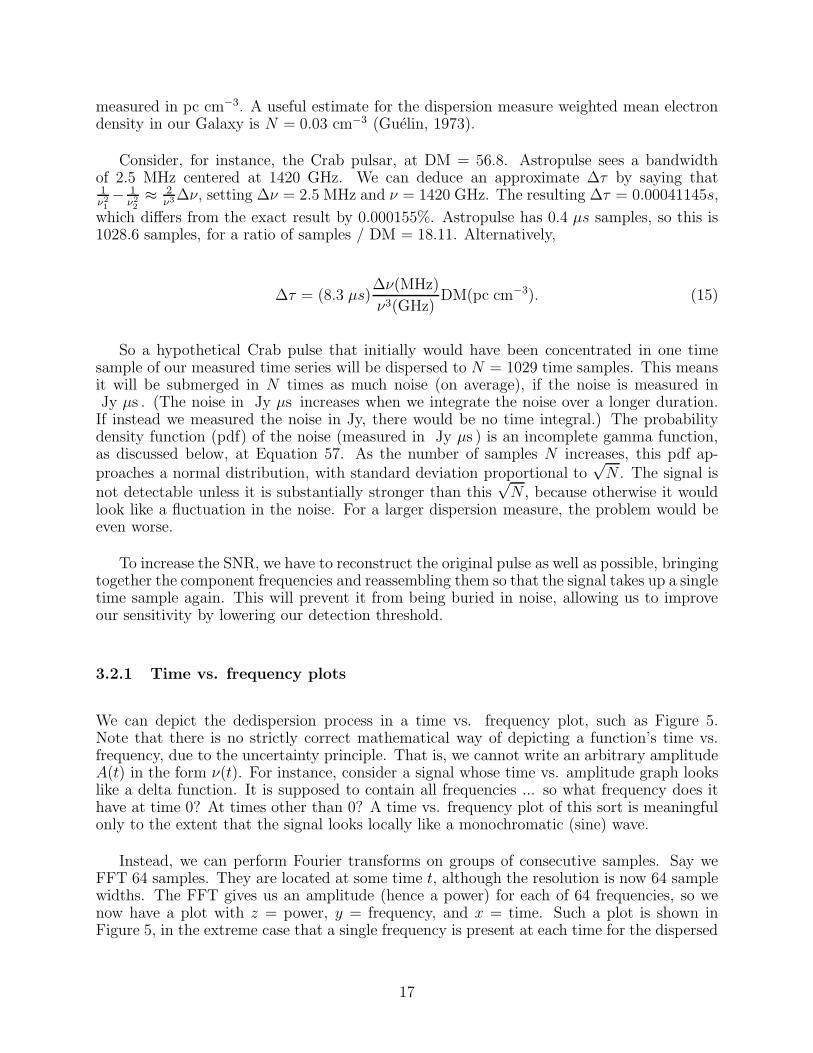
Instead, we can perform Fourier transforms on groups of consecutive samples. Say weFFT 64 samples. They are located at some time t, although the resolution is now 64 samplewidths. The FFT gives us an amplitude (hence a power) for each of 64 frequencies, so wenow have a plot with z = power, y = frequency, and x = time. Such a plot is shown inFigure 5, in the extreme case that a single frequency is present at each time for the dispersed

17

signal (i.e. there is no noise.) In this plot, the power is represented by the darkness of eachpixel.

Figure 5: The diagonal line represents the initial, dispersed signal. The vertical line is thededispersed signal. The x axis is time in Astropulse samples, and the y axis is frequency inMHz. The pulse has a dispersion measure (DM) of +50 pc cm−3 . This figure depicts lineardedispersion, as opposed to the nonlinear dedispersion dicussed in Section 3.2.5

3.2.2 Incoherent dedispersion and its limitations

We have two choices for our methodology: coherent dedispersion and incoherent dedisper-sion. Astropulse uses coherent dedispersion, whereas other radio surveys use incoherentdedispersion. Incoherent dedispersion is much more computationally efficient, and for longertimescales it’s almost as good as coherent dedispersion. However, as we will see, Astropulsewould be unable to examine the 0.4 µs timescale without coherent dedispersion.

Incoherent dedispersion means that the signal’s power spectrum is calculated, and thepower vs. time of each sub-band is analyzed. The method is called “incoherent” for thisreason – the phase information about individual frequencies is lost; only the total powerof each subband is retained. Next, the sub-bands are realigned at all possible dispersionmeasures, in an effort to find one DM at which the components align to produce a largepower in a short period of time. Suppose we use ∆τ to denote the difference betweenthe time delay of the highest and lowest frequencies in our bandwidth, as above. If ourincoherent dedispersion algorithm makes a linear approximation, then the sub-band withfrequency ν0 + ν (where ν0 is the center frequency) is shifted by a time ν

∆ν· ∆τ , where ∆ν

is our bandwidth.

However, incoherent dedispersion is limited in two ways. First, the goal of recording

18

power vs. time makes sense only on a timescale greater than dt1 = 1dν

, where dν is the widthof each sub-band. This is because of time-frequency uncertainty. Second, in each sub-bandthe pulse is dispersed by dt2 = ∆τ · dν

∆ν. So the method cannot localize the pulse better than

this. Setting dt = dt1 = dt2, we find that the minimum timescale for incoherent dedispersion,dt, happens when:

∆τ · dν

∆ν=

1

dν(16)

dν2 =∆ν

∆τ(17)

dν =

√

∆ν

∆τ(18)

dt =

√

∆τ

∆ν(19)

=

√

411 µsDM

56.8· (1.42 GHz

ν0

)3(∆ν

2.5 MHz) · (∆ν)−1 (20)

= 12.8 µs (DM

56.8)0.5(

ν0

1.42 GHz)−1.5. (21)

For the Crab pulsar, this is a limit of 12.8 µs , or 32 samples. For a more distant source,the limit might be as much as 50 µs, or 124 samples. (Astropulse considers sources with aDM as high as 830 pc cm−3 .)

3.2.3 Coherent dedispersion as deconvolution

Coherent dedispersion is an alternative technique that allows better time resolution, by per-forming the mathematical inverse of the ISM’s dispersion operation. Coherent dedispersiondeals with amplitude rather than power, preserving phase information; in the absence ofnoise or scattering, it would reconstruct the original pulse exactly. We need to analyze themathematical operation corresponding to dispersion, in order to find its inverse.

If F (n) is the original pulse as a function of sample number n, then suppose D[F ] is thedispersed pulse. We can show that D is just a convolution. In particular, D[F ] = F ∗ D[δ],where ∗ is convolution and δ is the discrete δ function.

We know that D is time translation-invariant and linear, because Maxwell’s equations ina plasma have these properties. That is, if we combine Maxwell’s equations with:

me~v = −e ~E (22)

~J = −ene~v (23)

19

for the velocity of the electrons (assuming the protons do not accelerate substantially),

we have a linear set of equations in ρ, ~J, ~E, ~B, and ~v. (These represent the charge den-sity, current density, electric field, magnetic field, and electron velocity, respectively.) Forexample, Figure 6 depicts a dispersed (chirped) delta function.

Figure 6: Delta function and chirped delta function. The x axis is time, and the y axisis amplitude. (Units are arbitrary for both axes.) Note that the chirped function tapersoff toward 0 amplitude at high and low times. This is because the initial function is nota true delta function; it has nonzero width. For an infinitely narrow delta function, thechirped function’s envelope would not taper off at all. Note also that our dedispersionoperation assumes that the band’s center frequency has a time delay of 0, with the highestfrequencies arriving earlier than an undispersed pulse would. Of course this is impossible;and our reconstruction of the pulse at this particular time is purely conventional. Thus, ourreconstructed pulse times are correct relative to other pulses of the same DM, but not in anabsolute sense.

When the delta function is time translated, so is the dispersed version (Figure 7.) Andwhen two delta functions are summed, so are the dispersed versions (Figure 8.) From figures7 and 8, we conclude that dispersion is linear and time translation invariant.

Then:

F (n) =∑

n′

F (n′)δ(n − n′) ≡ (F ∗ δ)(n), (24)

D[F ](n) =∑

n′

F (n′) · D[δ](n − n′) ≡ (F ∗ D[δ])(n), (25)

where the last step is by linearity and time translation invariance of D.

20

Figure 7: Time translated chirped delta functions. The x axis is time, and the y axis isamplitude. (Units are arbitrary for both axes.)

Figure 8: Two chirped delta functions. The x axis is time, and the y axis is amplitude.(Units are arbitrary for both axes.)

3.2.4 Coherent dedispersion using FFTs

Now the pulse that arrives at our detector is the output pulse F ∗ D[δ], and we want todetermine F . To do this, we use the fact that the convolution operator is related to the

21

Discrete Fourier Transform (DFT). We have DFT(f ∗ g) = DFT(f) · DFT(g)

Therefore

DFT(D[F ]) = DFT(F ∗ D[δ]), (26)

= DFT(F ) · DFT(D[δ]). (27)

We divide both sides of Equation 27 by DFT(D[δ]), and apply the inverse DFT, obtaining:

F = DFT−1(DFT(D[F ])

DFT(D[δ])). (28)

Convolution “the slow way” takes time O(N2) – that is, convolution by multiplying everyvalue of one function by every value of another function, then adding up the results. But theFFT is faster, taking time O(N log N), where N is the length of the FFT. (“DFT” refers to amathematical function, and “FFT” refers to a specific type of algorithm that computes thatfunction quickly.) For every N samples, coherent dedispersion takes time O(MN log N),where M is the number of dispersion measures to test. If L is the number of samples in thedata stream, coherent dedispersion takes time O(ML log N).

On the other hand, incoherent dedispersion does not test as many dispersion measuresas coherent dedispersion does, because its time resolution is imperfect and it cannot alwaysdistinguish between different DMs. To distinguish between two dispersion measures, the al-gorithm would have to notice that the pulses’ respective slopes differ in a time vs. frequencyplot. But if the pulses’ slopes differ by a very small amount, time-frequency uncertaintymay prevent us from detecting the difference. (And recall that time-frequency uncertaintyis a more significant problem with incoherent dedispersion, because the sub-bands are nar-rower than the full bandwidth.) Another consideration that limits time resolution, therebydegrading the precision of our DM detection, is dispersion within sub-bands.

Together, these two effects result in some practical time resolution of n samples, allowingus to test not M , but M/n dispersion measures. The value of n can be calculated fromEquation 21. For example, with a resolution of 20 µs and a sample duration of 0.4 µs ,n = 50. For each dispersion measure, we must process L samples, so we require timeO(ML/n). (Some additional time is required to FFT the data into a power spectrum, butthis process is not dominant.) So the time ratio between coherent and incoherent dedispersionis O(n logN). In our case, log N = 15, so this goes like 50 ·15 = 750, a large ratio. Of coursewe can’t calculate the ratio exactly, without knowing the respective constant factors. Butthis helps explain why coherent dedispersion is not generally used for surveys.

22

3.2.5 Computing the nonlinear chirp function

To find the chirp function DFT(D[δ]), we must first find D[δ]. This is just the chirped deltafunction. Although it is common to make a linear approximation to the chirp function, wewill make no such approximation, resulting in a nonlinear chirp function. We will find t(ν),the arrival time of frequency ν, and ν(t), the frequency arriving at time t. Then we willuse these functions to compute the frequency domain amplitude of the chirp function in twoways, a less rigorous way and a more rigorous way.

Now, the arrival time of frequency ν is given by Equation 14 as:

t(ν) =A

ν2+ t0. (29)

Thus, for interstellar dispersion, we expect higher frequencies to arrive first, which agreeswith Equation 29 for A > 0. We want ν = 1420 MHz to arrive at time 0, which requiresthat t0 < 0.

Let’s determine ν(t), the frequency arriving at time t. This has:

t =A

ν2+ t0, (30)

ν(t) = A1/2(t − t0)−1/2. (31)

Then

f(t) = exp(2πi

∫ t

0

ν(t′)dt′) (32)

is the pulse amplitude D[δ] as a function of time, if ∞ frequency arrives at time t0. We

want to find the chirp function DFT(D[δ]) = f(ν), so we can divide by it, as in Equation 28.We will calculate the chirp function in two ways.

For the first way, consider that we have defined the frequency ν(t) arriving at time tto be the time derivative of the exponent of the time-domain amplitude; see Equation 32.Let’s assume (without rigorous justification) that the function’s inverse t(ν) is the frequencyderivative of the exponent of the frequency-domain amplitude. (Where the frequency-domainamplitude is defined to be the Fourier transform of the time-domain amplitude.)

In that case, we can find the exponent of the frequency-domain chirp function simply byintegrating Equation 30. Define

23

ν0 = ν(0) = A1/2(−t0)−1/2 = 1420 MHz. (33)

Then

t(ν) = −A(1

ν2− 1

ν20

). (34)

The minus sign on the right hand side has been inserted due to some details of theFourier transform; the specifics will be given in the second derivation, below. We can findthe exponent of the frequency-domain amplitude by integrating this equation; we get:

∫

t(ν) = A(1

ν+

ν

ν20

+ C) (35)

= A(ν2

0

νν20

+ν2

νν20

+ Cν2

0ν

νν20

) (36)

= A(ν − ν0)

2

νν20

. (37)

where we have judiciously chosen C = −2 to simplify the equation. This results in afrequency domain amplitude:

f(ν) = exp(2πiA(ν − ν0)

2

νν20

). (38)

This is an easy way to get the correct answer. However, we have proceeded here froman assumption that t(ν), defined to be the inverse function of ν(t), is the derivative of the

exponent of f . But this is technically speaking not the definition of f . To quantitativelyjustify this result will take a bit longer. We can go back to the definition:

f(ν) =

∫ ∞

−∞f(t) exp(−2πitν)dt (39)

=

∫ ∞

−∞exp(2πi(

∫ t

0

ν(t′)dt′ − νt))dt. (40)

We evaluate this integral using the method of steepest descent, which is used to calculatean integral of the form

24

∫ ∞

−∞eg(t)dt. (41)

3.2.6 Method of steepest descent: justification

How can we show that we are justified in applying the method of steepest descent? Themethod is typically considered valid if g = 0 at some t = t, and the path of integration canbe arranged so that ℜ(g), the real part of g, has a global maximum (along the path) at t.Also, the third and subsequent derivatives of g should be small enough that g can be treatedas quadratic, at least until ℜ(g) becomes much smaller than its maximum. Then eg(t) canbe treated approximately as a Gaussian.

In our case g is pure imaginary along the path of integration, leading to an oscillatingcomplex exponential term. So we cannot have ℜ(g) smaller than the maximum, although itis conceivable that we could achieve this by changing the path of integration. But instead,let’s show that eg(t) can be treated as a Gaussian anyway. A rapidly oscillating term is small,so the right and left “tails” can be ignored; for instance, what is

∫ ∞t1

cos(g(t))dt where g(t)

and g′(t) are monotonically increasing? We can change variables like dt = t′(g)dg to get∫ ∞

g1

cos(g)t′(g)dg. Then t′(g) is monotonically decreasing, so that each half-period integral of

cos(g) is smaller than the previous. Since these integrals alternate in sign, the whole integralis on the order of t′(g1) = 1/g′(t1) = 1/ω1, if ω1 is the initial frequency.

In Equation 49, we will calculate that the magnitude of the integral in Equation 41 is√

2Aν3 . We want to show that the sizes of the left and right tails are much smaller than

that, so that we can ignore them. The “tail” is the non-Gaussian part of the integrand of

Equation 41. Roughly, we want 1/g′(t) ≪√

2Aν3 by the time any derivatives matter that

are higher order than g′′(t). First, let’s find the region in which the third and higher orderderivatives don’t matter. Note that ν is a constant throughout this calculation, as we arecomputing f(ν) for some particular value of ν. But ν(t) refers to something entirely different;it is a function of t. Then:

g(t) = 2πi(

∫ t

0

ν(t′)dt′ − νt), (42)

g′(t) = 2πi(ν(t) − ν) = 2πi(A1/2(t − t0)−1/2 − ν), (43)

g′′(t) = −πiA1/2(t − t0)−3/2, (44)

g′′′(t) =3

2πiA1/2(t − t0)

−5/2. (45)

The g′′′(t) term in the Taylor series expansion is insignificant as long as

25

|14πA1/2(t − t0)

−5/2(t − t)3| ≪ 1. (46)

Then

ν = ν(t) = A1/2(t − t0)−1/2, (47)

so we require

|14πν5A−2(t − t)3| ≪ 1,

|t − t| ≪ (4

π)1/3ν−5/3A2/3.

A = 4 · 1015 Hz · DM ( pc cm−3 ), so for a DM of 200 pc cm−3 , this last RHS is on theorder of 5 · 10−4 s.

We want to know whether 1/g′(t) ≪√

2Aν3 for all points outside this region. Then

g′(t) = 2π(A1/2((t − t) + (t − t0))−1/2 − ν), and suppose t − t = ǫ is small compared with

t0 = −0.41 s.

Now, ν ≈ ν0, so that t = t(ν) ≈ 0 and therefore t − t0 ≈ −t0. This means that ǫ is alsosmall compared with t − t0. So

g′(t) = 2πA1/2(t − t0)−1/2(1 − 1

2

ǫ

t − t0− 1)

= −πA1/2 ǫ

(t − t0)3/2

= −πǫν3

A1/|g′(t)| = 8.9 · 10−10.

In the last step, above, we have set ǫ = 5 · 10−4 s, so that we are considering a point onthe boundary of our region, where g′′′(t) is becoming important. Furthermore,

√

2A

ν3≈ 1.7 · 10−6. (48)

26

So 1/g′(t) ≪√

2Aν3 as desired. This suggests that for more extreme values of t, where g′′′(t)

starts to become important, the integral of the oscillating amplitude becomes insignificant.We are probably justified in applying the method of steepest descent, and treating theintegrand as a Gaussian.

3.2.7 Method of steepest descent: result

The method of steepest descent says that the value of the integral is:

±√

2π

|g′′(t)| exp(g(t)). (49)

The factor in front is just ±√

2π|g′′(t)| = ±

√

2Aν3 using Equations 44 and 47. Then we

consider the next factor,

g(t) = 2πi(

∫ t

0

ν(t′)dt′ − νt)

ν(t′) = A1/2(t − t0)−1/2

∫ t

0

ν(t′) = A1/22(t − t0)1/2|t0

t =A

ν2+ t0

∫ t

0

ν(t′) = A1/2 · 2(A

ν2)1/2 − 2A1/2(−t0)

1/2

= 2A1/2(A1/2

ν− (−t0)

1/2)

g(t) = 2πi(2√

A[

√A

ν− (−t0)

1/2] − ν[A

ν2+ t0])

= 2πi(A

ν− 2

√A(−t0)

1/2 − νt0).

Then, using Equation 33:

(−t0)−1/2 = A−1/2ν0,

t0 = −Aν−20 ,

27

g(t) = 2πi(A

ν− 2

√A√

Aν−10 + νAν−2

0 ),

= 2πiA(ν − ν0)

2

νν20

Since ν ≈ ν0 in our application, the chirp function looks something like exp(2πiA (ν−ν0)2

ν3

0

),

and the exponent would be a quadratic. But the extra factor ν0/ν is easily included in ourdedispersion algorithm, so we have done so. This extra factor gives rise to a curvature in thetime vs. frequency plot of the dispersed pulse, which must be on the order of (ν − ν0)/ν0,or in our case 1.25 MHz/1.42 GHz = 0.00088, which is about 1 sample out of every 1000.Therefore, this curvature could be quite significant for small coadds, especially for large DM.

3.3 Algorithm logic

Astropulse loops through the data at several nested levels. We consider DMs ranging from−830 pc cm−3 to −49.5 pc cm−3 , and from 49.5 pc cm−3 to 830 pc cm−3 .

In the list below, each single iteration of loop N involves several iterations of loop N +1.For instance, running on one large DM chunk entails running on 8 small DM chunks, eachof which involves running through all 2,048 chunks of the time series data.

1. Large DM chunk: blocks of 128 DMs at a time.

At the highest level of the nested loop structure, Astropulse considers groups of 128DMs at a time, analyzing the entire 13s workunit at all of these DMs. At the endof each large DM chunk loop, Astropulse runs the modified fast folding algorithm(Section 3.3.1) on the entire data set, with a resolution of 128 samples.

1.a Small DM chunk: blocks of 16 DMs at a time.

Every time Astropulse completes 16 DMs, we say that it has finished a small DMchunk. At the end of each small DM chunk, Astropulse runs the modified fast foldingalgorithm on the first 1,048,576 = 220 samples of data, with a resolution of 16 samples.

2. Data chunks of size 32,768 = 215 samples.

In order to analyze the data using a set of 16 consecutive DMs, Astropulse divides thetime series into data chunks of size 215 samples. However, the starting points for thesedata chunks occur every 214 samples; there is a 50% overlap. So each piece of the timeseries is analyzed as the first half of one data chunk, and the second half of another.The 50% overlap can catch some pulses that would otherwise extend beyond the edgeof a data chunk; part of the dispersed pulse would exist in one data chunk, and partin another. We want to operate on the whole pulse with a single Fourier transform.

Within this loop, we compute the Fast Fourier Transform (FFT) of the data for usein convolution, producing a frequency spectrum that will later be dechirped and thenFFT’ed in reverse.

28

But the precise DM is not chosen until a lower-level loop. Why are we allowed tocompute the FFT before we have decided on a DM? Recall that each deconvolutioninvolves two FFTs, one forward and one backward. The DM determines the chirpfunction, which is applied after the forward FFT. Therefore, we can don’t have toperform the forward FFT once for every single DM.

3. All DMs within a small DM chunk.

When considering one 215 sample data chunk, Astropulse runs through the current 16DMs individually.

4. Sign of the DM (positive and negative).

We consider negative DMs for a few reasons:

(a) Extraterrestrial civilizations might communicate using signals dispersed with neg-ative DMs.

(b) Signals detected at both positive and negative DM can be a sign of radar or otherradio frequency interference (RFI).

5. Scales (or “co-adds”) 0 − 9.

Scale (or co-add level) ℓ means that the client combines 2ℓ adjacent samples and mea-sures the total power. This allows us to search for pulses of any width, ranging from0.4 µs (1 sample) to 204.8 µs (512 samples.)

6. Samples within the data chunk

If the power in 2ℓ samples is above a certain threshold, then Astropulse reports a pulse.

3.3.1 A modified folding algorithm

To search for periodic pulses, we employ a folding algorithm, inspired by the Fast FoldingAlgorithm (FFA) of Staelin (1969). Staelin’s algorithm searches efficiently through a seriesof nearby periods. (Say, periods of 3, 31

3, 32

3, and 4.) Our modified folding algorithm, on the

other hand, searches efficiently through a series of periods that differ by successive factorsof 2. (For instance, periods of 12, 6, 3, and 11

2.) The modified algorithm is described in

Korpela et al. (2000), and can be summarized as follows.

Before folding, we collapse our data in the time domain by summing either 16 or 128samples, depending on whether it was created during the large or small DM chunk loop.Below, a collapsed set of samples will be called a “bin.” The FFA has several nested loops;each single iteration of loop N generally involves many iterations of loop N + 1:

1. Loop over frequencies

We define the frequency to be the number of periods over the entire time series. Thesmallest frequency in this loop is always Fmin = 137, and the largest frequency is twicethat. The frequency increments via multiplication by (1 + 1

N), where N is the number

of bins in the sub buffer.

29

We construct a new, shorter time series from the original time series, by folding it.That is, we divide the time series into F chunks, where F is the frequency, and addthem up.

2. Loop over subfrequencies

This part is what makes the folding “fast.” Instead of re-folding at all frequenciesgreater than 2Fmin, we simply fold frequency F in half to make 2F , again to make4F , and so on.

3. Loop over co-adds

As in the single pulse algorithm, we search for pulses that take up more than onebin. In this case, of course, a single bin could be 128 samples, two bins would be 256samples, etc.

4. Loop over bins

Examine each bin to see if the power exceeds the threshold, see 3.4.

We can compute the dependence of the run time on N , the number of bins, as follows.

1. We must search O(N) frequencies, since the frequencies differ by the ratio (1 + 1N

).

2. We must search O(N) bins (or phases of the repeating signal) for each frequency.

This makes an overall O(N2). The run time is also influenced by the number of timeswe run the modified folding algorithm. (E.g. once every 128 DMs or every 16 DMs.)

3.4 Thresholds

Astropulse searches for pulses whose power exceeds certain thresholds. These thresholdscan be calculated either experimentally or theoretically. I’ll start by finding the theoreticalvalues, then point out some of the uncontrollable factors that make these values inaccurate,and finally I’ll describe the experimental methods for calculating thresholds.

3.4.1 Single pulse thresholds: theory

We want to calculate the distribution (pdf) of the integrated noise power in 2ℓ samples, afterdechirping. (Here, the power refers to the absolute value of the square of the amplitude,where the undispersed time series has amplitudes ±1.)

First, we assume that the pre-deconvolution time series is pure white noise; that is, eachbit of a two bit complex sample is independently distributed with equal probability of a 0

30

or 1, so each f(t) has equal probability for ±1 ± i. Then we deconvolve this data by FFT.In other words,

f(k) =1√N

N−1∑

t=0

f(t)e−2πikt/N . (50)

The distribution of a single f(k) is Gaussian (by the central limit theorem), and the

variance of ℜ(f(k)) comes from the sum of the 2N variances of the ℜ(f(t)) and ℑ(f(t)), or2N( 1√

N)2E(sin2) = 1. We will then multiply by a chirp function which looks like eiphase(k),

and doesn’t affect the individual variances. Finally, we run the inverse FFT. We assumethat the chirp function has scrambled the phases, so that the result is once again a sumof independent and identically distributed (iid) random variables. The previous argument

applies, and since the variances of ℜ(f(k)) and ℜ(f(t)) are both 1, we get the same resultas before: a standard Gaussian, σ = 1.

The power in each sample after deconvolution will be distributed like |ℜ(f(k))|2 +

|ℑ(f(k))|2, the sum of the squares of two standard Gaussians. This distribution is easilycalculated; the joint distribution is:

1√2π

ex2

2 · 1√2π

ey2

2 dxdy (51)

=1

2πe−

r2

2 rdrdθ (52)

→ e−r2

2 rdr (53)

= e−udu. (54)

where u = x2+y2

2is half the power in one sample, in the time domain. Therefore, half the

power is exponentially distributed with mean 1; or equivalently, the power is exponentiallydistributed with mean 2.

In future calculations, we will normalize to half of this power, so that the average powerper sample is 1.

So for instance, if after dechirping we find that a certain sample has a power of 15.3, weconclude that only one in e15.3 samples has a comparable power. To ascertain how unlikelythis is, we need to calculate how many such samples we have examined over the entire courseof the experiment. This would be:

48 TB × 4 · 1012 samples per TB × 14208 DMs

× 2 DM signs × 2 from co-adds

= 1.09 × 1019 = e43.8. (55)

31

(Co-adds cause a factor of 2 because there are half as many potential pulses at eachco-add, compared with the previous co-add. So 1 + 1

2+ 1

4+ . . . + 1

256≈ 2.)

With a threshold of 43.8, we would rule out all but one noise pulse over the course ofour entire observation history. However, it seems more prudent to allow one noise pulse perworkunit, and sort out false pulses later.

In this case, we just want:

225 samples per workunit × 14208 DMs × 2 signs × 2 from co-adds = e28.3. (56)

When we collapse n = 2ℓ samples to make one bin, we are adding up that many expo-nential distributions. The result is a gamma distribution, with scale parameter 1 and shapeparameter n. The pdf is

1

Γ(n)xn−1e−x. (57)

and the cumulative distribution function is

γ(n, x)

Γ(n). (58)

where γ is the incomplete gamma function. The first few pdfs are shown in Figure 9.

3.4.2 Expected discrepancies with the model

A few differences from the model can be expected:

1. Hydrogen line and filter shape. We assumed above that the input data is whitenoise. In practice, this is not the case, because a portion of our band has higher powerdue to the hyperfine hydrogen line. The strength of this line can vary depending on ourRA and dec. Then f(k) no longer have equal standard deviations. This will cause somecorrelation between the deconvolved power of adjacent samples, which will modify thepdf of the binned power, increasing the variance.

To see this, consider the simplest, most extreme case, where the hydrogen line is astrong delta function of amplitude A at frequency k0, where A is distributed randomlylike a Gaussian with standard deviation σ. Then if f is the dechirped amplitude,f(t) = Ae2πik0t/N . (The dispersion is not relevant, since the hydrogen line has asingle frequency.) So |f(t)|2 is exponential with power σ2. But |f(t1) + f(t2)| is

32

Figure 9: Gamma distributions. The x axis is integrated power (divided by 2, as per ourconvention), and the y axis is probability per unit power. The leftmost distribution, which isexponential, belongs to n = 1. The rest are n = 2, 4, 8, 16, 32, 64. Notice that the rightmostdistribution is nearly a normal distribution.

A|e2πik0t1/N +e2πik0t2/N |. If t1 ∼ t2, this is roughly 2A, which is Gaussian with standarddeviation 2σ and variance 4σ2. Whereas if we summed samples without the hydrogenline, adding identical and independently distributed (iid) exponentials, the varianceswould simply add to give 2σ2. So this model hydrogen line increases the variance.

In actuality, the effect of the hydrogen line is not so pronounced, but the idea is similar.In the same way, the nonuniform shape of our low pass filters also causes the signal todiffer from white noise.

2. Other disparities

Even in the absence of the hydrogen line, tests reveal other differences between thetheoretical and actual distributions. For larger bin sizes, the variance is less thanexpected.

It’s easy to see that power per sample cannot be independently distributed, even inthe case of white noise. This is because the total power over all samples must be aconstant; in our case, the constant is 32768 = 215, the total number of samples in aFFT. This would certainly result in a smaller variance, but we have not establishedwhether this effect suffices to explain the observed disparity.

3.4.3 Repeating pulse thresholds: theory

For repeating pulses, the situation is simpler. We test a repeating pulse by adding up Msamples, where M is very large. These samples are not all consecutive. For the minimum

33

value of M , we add groups of 16 samples together, with a frequency of Fmin = 137, for atotal of M = 16 ·137 = 2192. This sum of many iid variables will have a normal distributionwith variance M and standard deviation

√M .

The total number of potential pulses per 13 s workunit is as follows.

1. Frequencies. Suppose the number of samples (which is 220 or 225) is n, and the DMchunk size (16 or 128) is d. Then there are L frequencies, where (1 + 1

n)L = 2. That

is, eLn = 2, so L = n · ln(2).

2. Phases. Each frequency has a period equal to about n/Fmin, and the phase of therepeating pulse can start at any point in that period.

3. Subfrequencies. Each frequency has a number of subfrequencies, each of which hashalf as many bins as the previous. This doubles the number of potential pulses.

4. Coadds. Each subfrequency has a number of co-adds, each of which has half as manybins as the previous. This doubles the number of potential pulses again.

5. Number of DM chunks. The FFA runs 14208d

times for each of 2 signs, where d isthe DM chunk size as above.

Therefore, the total number of potential pulses is

n · ln(2) · (n/Fmin) · 4 · (14208/d) · 2 = (n2 · 8 · ln(2) · 14208)/(Fmin · d3), (59)

which is 3.09× 1011 = e26.5 for the large DM chunk, and 1.54× 1011 = e25.8 for the smallDM chunk.

We want the number of standard deviations such that the probability of exceeding thatnumber is e−26.5 or e−25.8, respectively. We can perform the integration in idl, finding thatwe need thresholds of 6.88σ in the large DM chunk case and 6.78σ in the small DM chunkcase, where σ =

√M .

3.4.4 Single pulse thresholds: experiment

To choose our thresholds for the single pulse search, we ran the client on 10 workunits,keeping track of the strongest pulses we found at each co-add. The second largest pulse outof 10 is roughly the 90th percentile, so we set our thresholds at that point. This methodgives thresholds that are reasonable as long as we don’t demand that we detect preciselyequal numbers of pulses at each co-add.

34

3.5 Expected sensitivity

3.5.1 Sensitivity of Astropulse

To calculate Astropulse’s expected sensitivity as a pulse area in Jy µs , we will follow thetreatments in (Rohlfs & Wilson, 2000) and (Van Vleck & Middleton, 1966). A signal froma telescope receiver consists of a function f(t) that describes the amplitude of the signal attime t. However, we will be discussing a generalization of a signal, called a “random process.”A random process is not a particular signal, but a probability distribution over the set of allsignals; it is a random variable whose values are signals. It is natural to talk about noise asa random process, since we do not know in advance the amplitude of the noise as a functionof time. The random process is associated with a probability density function (pdf) on thespace of all signals. Because the signals are functions, this pdf is a function on a domain offunctions; so we could call it a functional. Such a functional could be written f [x(t)], wherethe function x : R → C is a signal with some amplitude at each time t. So for instance, therandom process would assign some probability density to the signal x1(t) = sin(t), and wouldassign some other probability densities to the signals x2(t) = 2 sin(t), x3(t) = sin(2t)−sin(t),and so on.

Another, equivalent way of thinking about a random process is that it can be writtenas X(t), which is a random variable for each value of t, not necessarily independent. (Twodifferent random variables need not be independent. For instance, the amplitude of thehyperfine hydrogen line at time t is a random variable, where we have applied a filter toisolate a narrow band around the desired frequency. The amplitude at time t + T , whereT = 1

νand ν is the frequency of the hydrogen line, is another random variable. But these

two random variables are not independent, and they will tend to have the same value if weare considering a narrow enough band.)

We will consider Gaussian random processes; namely, processes X which can be writtenas a sum like:

X(t) =∑

ν

Aν(Zν + iZν)e2πiνt, (60)

where Aν are positive real constants, and Zν , Zν are random variables distributed inde-pendently as real Gaussians with σ = 1, µ = 0. For such processes, the value X(t) for any tis distributed as a complex Gaussian with variance

∑

ν A2ν in the real and imaginary compo-

nents. But although Zν are independent, X(t1), X(t2) may not be independent. In general,there is some correlation coefficient r such that the joint pdf of the real (or imaginary)components of X(t1), X(t2) is:

p(x1, x2) =1

2π√

1 − r2exp(

1

1 − r2(x2

1 − 2rx1x2 + x22)). (61)

To calculate Astropulse’s sensitivity, we want to relate the following quantities. Subscript

35

0 refers to the signal emitted by the receiver and entering the one-bit sampler. Subscript 1refers to the signal emitted by the one-bit sampler.

F = the signal flux entering the telescope (from an astrophysical source).

G = the gain of the telescope, in K Jy−1.

kT0 = the average noise power emitted by the receiver, per unit bandwidth, andentering the one-bit sampler.

S0 = the average signal power emitted by the receiver and entering the one-bit sampler.

P1 = the average noise power emitted the one-bit sampler, in dimensionless units.

S1 = the average signal power emitted by the one-bit sampler, in dimensionless units.

We will assume, for simplicity, that the power S0 comes from a signal with amplitudeX0(t) = A(Zν0

+ iZν0) exp(2πiν0t) for a single ν0. We require that E(|X0|2) = 2A2 is the

average power S0, where E denotes expected value. The Gaussian distribution may seemincorrect – it allows the possibility of zero signal power, for instance. But it turns out thatwe can calculate the precise effect of the sampler on the signal X0, so we will make thatcalculation and then assume that the nonzero expected power is what’s important.

Next, we consider autocorrelations, and their relationship with power spectra. The au-tocorrelation RX(τ) is a property of a random process X(t), and has a delay parameter τ .It measures the correlation between the signal at time t and at time t + τ . It’s defined by:

RX(τ) ≡ E(X∗(t)X(t + τ)). (62)

The autocorrelation is useful in several ways. The simplest is that RX(0) = E(|X(t)|2),the expected power. Another fact is that the Fourier transform of R is the same as the powerspectral density (PSD) S(ν). The PSD is defined as the expected value of the square of the

amplitude in the frequency domain, S(ν) ≡ E(|X(ν)|2) = 2|Aν |2.

Now we compute RX0, the autocorrelation of X0:

RX0(τ) ≡ E(X∗

0 (t)X0(t + τ)) (63)

= 2A2exp(2πiν0τ) (64)

= S0 exp(2πiν0τ), (65)

where the last step is consistent with the fact that RX0(0) must equal the signal power S0.

Now the total power emitted by the receiver is kT0B + S0, which comes from a signal withamplitude Y0(t) + X0(t), where Y0(t) is white noise. Since Y0 and X0 have a random phase

36

relationship, the autocorrelation function of the sum is just the sum of the autocorrelationfunctions. (That is, E(X∗

0 (t)Y0(t + τ)) = E(Y ∗0 (t)X0(t + τ)) = 0). Then the noise is not

correlated with itself over long time scales τ , so RY0, the autocorrelation of Y0, is:

RY0(τ) = E(Y ∗

0 (t)Y0(t + τ)) (66)

= kT0Bg(τ), (67)

for some narrow function g(τ). The total noise power is E(|Y 20 |) = RY0

(0), which mustbe equal to kT0B, where B is the bandwidth. Therefore g(0) = 1. So

R0(τ) = kT0Bg(τ) + S0 exp(2πiν0τ). (68)

We need to characterize the output signal that results from clipping R0. This problem isconsidered in (Rohlfs & Wilson, 2000) and (Van Vleck & Middleton, 1966). In the case ofa Gaussian signal, the joint pdf of amplitudes at any two times (i.e. X0(t1), X0(t2)) takes aclosed form as above. From that form, one can derive the correlation between the probabilitythat the clipped noise will be ±1 at t1 and t2. Then one can write down the autocorrelationfunction of the clipped noise. For the real bits alone, the autocorrelation is:

R1(τ) =2

πarcsin

(

R0(τ)

R0(0)

)

. (69)

As expected, the power is R1(0) = 1. For the real and complex bits together, theautocorrelation must be twice as large, R1(0) = 2. For S0 ≪ kT0B, the total power ismostly due to the noise kT0. However, at values τ 6= 0, the contribution of g(τ) falls offquickly. Therefore,

R1(τ) = 2 · 2

πarcsin

(

S0 exp(2πiν0τ)

kT0B

)

(70)

≈ 2 · 2

π

S0 exp(2πiν0τ)

kT0B, (71)

where we are ignoring R1(0), because g(τ) is narrow and we are only going to use R1(τ)in an integral. The power at frequency ν0 is found by integrating

S1(ν) =

∫

R1(τ)e−2πiντdτ = 2 · 2

πδ(ν − ν0)

S0

kT0B. (72)

37

which says that the total power near ν0 is∫

S1(ν)dν = 2· 2π

S0

kT0B. Then the ratio

S1,near(ν0)

R1(0)=

2π

S0

kT0B. In other words, S1/P1 = 2

πS0/P0.

As discussed above, in Section 3.4.1, the integrated power has a gamma distribution,both in the frequency domain and (when dechirped) in the time domain. To summarize theresults from that section: in the absence of any input signal S0, the frequency components’amplitudes should behave like Gaussian variables. So after a discrete Fourier transform,P1(ν0) has an expected power of 2, and is distributed as a sum of the squares of two Gaussians(real and imaginary.) This distribution could be seen as a chi squared with 2 degrees offreedom, a gamma distribution, or an exponential distribution. In the time domain, ifwe dedisperse the noise by performing a Fourier transform, dividing by a chirp function(dechirping), and then performing the inverse Fourier transform, we should still end up witha sum of a real and a complex Gaussian. This should give us an exponential distribution foreach time sample.

Now assume that a chirped pulse with energy E0 emitted by the receiver will have

2

π(

E0

kT0Btsample

) (73)

times the expected power in one sample after the one-bit sampler. (This assumption isreasonable, since a chirped pulse looks like a monochromatic signal locally. Therefore wecan apply the above reasoning, even though our proof was for monochromatic signals.) Theintegrated noise will have N times the expected power of one sample, where the duration ofthe pulse is N samples, so the pulse will be detectable if

(2/π)E0 + kT0BNtsample

kT0Btsample(74)

is above threshold for N samples, where the threshold comes from a chi squared with2N degrees of freedom. Astropulse sets this threshold to H ∼ 30 for N = 1 sample, asdiscussed in Section 3.4.1. Since the pdf of the noise power is exponential, this excludes allbut a fraction e−H of the noise.

Then the minimum detectable energy satisfies the equation:

2

πE0 + kT0BNtsample = kT0BtsampleH (75)

2

πE0 = kT0Btsample(H − N) (76)

E0 =π

2kT0Btsample(H − N) (77)

E0 =π

2kT0(H − N) (78)

38

using the fact that Btsample = 1. If a signal is detected with H times the average

power in one sample, the implied energy of the pulse can be determined by inserting H intoEquation 78.

We have calculated E0, the value of the energy emitted by the receiver. This impliesthat the signal has a power per bandwidth of E0/(BNtsample) = E0/N , hence a temperatureof T = E0

Nk. This means the astrophysical source has a flux of T/(2G) = E0

2GNkin this

polarization. (By definition of the gain.) If it is actually unpolarized, the total flux in bothpolarizations is twice that, or T/G. Then its pulse area is:

F · (Ntsample) =E0tsample

Gk=

π

2

T0 tsample(H − N)

G. (79)

This value could be measured in Jy µs , for instance. In our case:

1. T0 ∼ 30 K is the system temperature.3

2. G = 10 K Jy−1 is the telescope gain, roughly equal to Ak, where:

3. A = λ2

Ωis the effective area of the telescope and k is Boltzmann’s constant.

4. λ = 21 cm is the wavelength of the signal.

5. Ω = 8.3 · 10−7 is the beam’s solid angle.

So the resulting flux density · duration is 1.9 (H − N) Jy µs .

3.5.2 Sensitivity comparison

While Astropulse detects a signal coherently, other undirected radio surveys use incoherentdetection schemes. Typically they use a filter bank, dividing the spectrum into N sub-bandsas described in Section 3.2. The method amounts to measuring the deviation ∆T from thereceiver temperature T0 at successive times, but in a different channel at each time. Thechannel frequency varies at a constant rate that is proportional to some dispersion measure(DM) that one is testing for.

First consider a single-channel device with bandwidth B. Then following Wilson et al.(2009), we assume the spectrometer finds the power in a band by Nyquist sampling at twicethe bandwidth, then finding the average of the squares. The square of a Gaussian with σ = 1is a chi squared with one degree of freedom, having a variance of 2. In this case, the powerP has µ = kT0B, so P = X2, where X is a Gaussian with σ =

√kT0B. Then P

kT0Bis a chi

squared with variance 2, and P has variance 2(kT0B)2. The variance of the 2Bt samples in

3http://www.naic.edu/alfa/gen_info/info_obs.shtml

39

time t is 2(kT0B)2(2Bt). Assuming we can detect a deviation of mσ, that’s m√

2kT0B√

2Bt.To find the standard deviation of the average power per sample, divide by the 2Bt samples toget mkT0B/

√Bt. Then find the equivalent temperature of this minimum detectable signal,

dividing by kB to get:

Teff = mT0/√

Bt. (80)

A multichannel filter spectrometer will have the same sensitivity, assuming it can addup the correct parts of the signal. This might be problematic in the cases of time-frequencyuncertainty or dispersion within sub-bands, as discussed in section 3.2. We can understandthese effects as widening the pulse width by a factor t

Wiwhile preserving the pulse area, so

that the effective temperature Teff is equal to Wi

tTint for an intrinsic temperature Tint. For

instance, Deneva & Cordes (2008) give the sensitivity formula as:

Tint = (t

Wi

)mT0

√

NpolBt, (81)

t = (W 2i + ∆t2DM,ch + ∆t2DM,err + ∆t2sc)

1/2. (82)

t is the effective width of the pulse,

Wi is the intrinsic width of the pulse,

∆tDM,ch is the dispersion within one channel, and is given by Equation 15,

∆tDM,err is the error caused by looking at the wrong dispersion measure, and can becalculated by inserting 1

2the DM step into Equation 15, using the whole bandwidth

as ∆ν,

∆tsc ∝ f−3.86 is the error caused by scattering broadening.

This assumes that the channel bandwidth is not so narrow that we are sampling beyondthe Nyquist rate. If the channel bandwidth were that narrow, there would be anothercontribution to the effective width; but all surveys are careful not to sample beyond theNyquist rate.

In any event, if one cares about the pulse area in Jy µs rather than the instantaneousflux, Equation 80 will suffice. One can calculate the area of a single polarization A = mT0t

2G√

Bt=

m T0

2G

√

t/B, or both polarizations together, A = mT0

G

√

t/B.

The most difficult variable to quantify above is perhaps tsc. We can estimate it using theempirical formula given in Lorimer & Kramer (2005):

log tsc,ms = −6.46 + 0.154(log DM) + 1.07(log DM)2 − 3.86 log νGHz. (83)

40

However, this formula applies to sources in the Milky Way. Astropulse spends a sub-stantial fraction of the time looking outside our Galaxy, in which case tsc should be muchsmaller, even for large DMs. But the distribution of the intergalactic medium is not wellunderstood. Lovell et al. (2007) find that extragalactic radio sources at redshifts greater thanz = 2 do not have microarcsecond structure, suggesting that they are scatter broadened byturbulence in the IGM. A microarcsecond of angular broadening at z = 2 corresponds to apulse width of τ = θ2d/c = 8 µs (using d = 3.57 Gpc). According to Ioka (2003), this is aDM of about 2000 pc cm−3 . So perhaps we can assume that at the (smaller) DMs of our ex-periment, pulses will have reasonably small widths. For instance, inside the galaxy, a DM of830 pc cm−3 would have a scattering width 400 times smaller than a DM of 2000 pc cm−3 .Even if the scattering width were nearly 8 µs , Astropulse is still good at detecting suchpulses. (The threshold is just twice as high as for 1 sample pulses.) Therefore, we will ignorethe scattering error in the tables below, and set t = tsample. In the tables, the followingconventions are observed:

• σ: number of standard deviations for threshold.

• tsample: the time resolution.

• t: the effective duration of the pulse after dedispersion.

• beam Ω: the telescope beam with, in steradians.

• beams: number of simultaneous beams.

• tobs: observation time per beam, in hours.

• dmax: the minimum distance from which an exploding M = 108 kg black hole wouldbe visible, in kpc. It’s calculated using

Umin = energy/(area · bandwidth) = (Mc2)/(4πd2max · 1GHz), (84)

where Umin is the minimum detectable signal in Jy µs .

• rate: the minimum rate of black hole explosions under which such a black hole wouldbe detectable, V −1t−1

obs. Here, V = (4π/3)d3nbeamsΩ4π

= 13Ωd3nbeams is the volume of

space observed at any one time.

I conclude that Astropulse’s minimum detectable rate (in black holes explosions pc−3

yr−1) is comparable to that of other surveys, but not superior. Astropulse’s rate is similar toLorimer & Bailes (2007) and Deneva & Cordes (2008). My sensitivity to unresolved pulses,in Jy µs , is superior to all other surveys listed except for Deneva’s. This sensitivity comeslargely from my microsecond time resolution and high gain. My observation time is alsosuperior. Astropulse does have substantial disadvantages, including a limited bandwidthand narrow (Ω = 8.1 · 10−7) beams. The rate limit and some of the other parameters inthese tables are plotted in Figures 27, 28, and 29, in Section 7.

41

Table 1: Survey parameters

# author telescope year dedisp ref ν0 (MHz) σ T0 (K) tsample(µs) t(µs)1 O’Sullivan et al. Dwingeloo 1978 incoh a 5000 6 65 2 27002 Phinney & Taylor Arecibo 1979 incoh b 430 6 175 1.7 · 104 1.7 · 104

3 Amy et al. MOST 1989 incoh c 843 6 - 1 1.7 · 104

4 Katz & Hewitt STARE 2003 incoh d 611 5 150 125000 1250005 McLaughlin et al. Parkes 2006 incoh e , f 1400 6 21 250 2506 Lorimer & Bailes Parkes 2007 incoh g 1400 6 21 1000 10007 Deneva et al. Arecibo 2008 incoh h 1440 5 30 64 648 Von Korff et al. Arecibo 2009 coher - 1420 30 30 0.4 0.4

# ∆ν (MHz) G (K Jy−1) beam Ω beams tobs (h) Npol sens ( Jy µs ) dmax (kpc) rate (pc−3yr−1 )1 100 0.1 6.6 · 10−6 1 46 1 2 · 104 100 8.4 · 10−8

2 16 27 6.6 · 10−6 1 292 1 1300 250 8.7 · 10−10

3 3 - 3.6 · 10−8 32 4000 1 1.6 · 105 i 22 5.4 · 10−8

4 4 6.1 · 10−5 1.4 1 13000 2 1.8 · 109 0.21 1.6 · 10−7

5 288 0.7 1.3 · 10−5 13 1600 2 120 810 1.8 · 10−13

6 288 0.7 1.3 · 10−5 13 480 2 240 580 1.7 · 10−12

7 100 10 8.1 · 10−7 7 420 2 14 2300 9.0 · 10−13

8 2.5 10 8.1 · 10−7 7 1460 1 54 1200 1.6 · 10−12

aO’Sullivan et al. (1978)bPhinney & Taylor (1979)cAmy et al. (1989)dKatz et al. (2003)eMcLaughlin et al. (2006)fManchester et al. (2001)gLorimer & Bailes (2007)hDeneva & Cordes (2008)iMOST has 1 mJy of noise in each beam after 12 hours, http://www.physics.usyd.edu.au/sifa/Main/MOST

42

4 Distributed computing : the BOINC platform

Astropulse runs on the BOINC platform (Anderson, 2004), an acronym for “Berkeley OpenInfrastructure for Network Computing.” BOINC is a set of programs that organizes vol-unteers’ home computers to perform scientific calculations. In a typical BOINC project,a researcher has a computing problem that can run in parallel, that is, on several ma-chines at once. Perhaps the problem involves searching a physical space (for Astropulse,this space is the sky), and performing the same computation on each point in that space(for Astropulse, this computation is dedispersion.) The first BOINC project, SETI@home,searched the sky for narrowband transmissions. The space could also be a parameter space,for instance a space of potential climate models (climateprediction.net) or protein configu-rations (Rosetta@home). The visible manifestation of a BOINC project is an informativescreen saver. Figure 10 shows the Astropulse screen saver, and Figure 11 depicts the cli-mateprediction.net screen saver.

Although the volunteers are providing their computers for free, the bandwidth and storagespace required to distribute data to the volunteers is not free. A project is suitable for BOINConly if it is computation-intensive. That is, the monetary cost to perform the computationmust be greater than the monetary cost of distributing the data. Coherent dedispersionsatisfies this requirement, because we must perform FFTs at many DMs.

Figure 10: The Astropulse screen saver.

43

Figure 11: The climateprediction.net screen saver.

The researcher for a BOINC project need not be affiliated with UC Berkeley, or with theBOINC development team at Berkeley (although we happen to be so affiliated.) BOINCis open source, and can be downloaded, compiled, and operated by anyone with sufficienttechnical skills; about 50 projects currently exist outside Berkeley.

Likewise, volunteers need not have any particular technical knowledge. They just haveto navigate to the BOINC web page with their web browser, and follow the instructionsto download the client programs described below. Astropulse has access to around 500,000volunteers, each of whose machines might have 2 GFLOPs of processing power, and be on1/3 of the time, for a total of 300 TFLOPs – as much as the world’s fastest general purposesupercomputer in 2007, IBM’s Blue Gene / L.5 Since that time, the processing power of thefastest supercomputer has increased to 1800 TFLOPs or more.6 Volunteer counts for eachproject, as well as other statistics, are compiled and displayed on web pages as shown inFigure 12 and Figure 13. Both images are from circa 2007.

Figure 14 depicts the parts of a BOINC project and the relationships between them.

1. Data: Astropulse, in particular, processes data in 8 MB workunits, which consist of

5http://www.top500.org/list/2007/06/1006http://www.top500.org/list/2009/11/100

44

Figure 12: Sample screen shot of statistics for all BOINC projects.

Figure 13: Sample screen shot of statistics for SETI@home.

1-bit complex sampled time series recorded at Arecibo.

45

2. Client code: runs on the volunteer’s machine.

(a) The application client code, written by the researcher who owns that particularproject. In the case of Astropulse, this is the code that performs the dedispersion.Because our code is open source, a few (< 1%) highly computer literate volunteersmake minor adjustments to this code in order to make it run faster on theirmachines. The validator (see below) ensures that the volunteers’ modificationsdo not alter the scientific results.

(b) The BOINC client code, written by the BOINC team at Berkeley. It relays thedata to the application client and performs monitor and control functions, suchas handling application client crashes.

3. Server code: runs on the researcher’s machines.

(a) The validator, written by the researcher, checks whether a given workunit pro-duces the same results when sent to different volunteers. This means that volun-teers can construct their own application clients without corrupting our data iftheir results are erroneous. This precaution also handles the hypothetical possi-bility that a volunteer would modify our client code for malicious reasons.

Care must be taken to understand what the validator does and does not permit. Ifvolunteers alter their pulses’ DMs, pulse areas, detection times, or other scientificparameters, the validator will notice and complain. However, the validator doesnot check bookkeeping information such as the client’s version id number, whichis not relevant to our scientific results.

(b) The assimilator, written by the researcher, records scientific results in a sciencedatabase.

(c) BOINC backend programs schedule workunits to be sent to different volunteers,run the validator and the assimilator, and record bookkeeping information in aseparate BOINC database.

In the case of Astropulse, preliminary versions of the application client, validator, andassimilator existed prior to my joining the project. This code was contributed by previ-ous members of the SETI@home research group, including Nopparat Pantsaena, RyohiTakahashi, Christopher Day, Karl Chen, Paul Demorest, and Eric Heien, all of whomhad left the group by the time I joined. I was responsible for causing these programsto run together for the first time by completing the client, and then augmenting allprograms as necessary. A copy of the final version of the application client can befound in Appendix B.

46

Figure 14: BOINC infrastructure. “Project back end” refers to the validator and assimilator.The scheduling server, utility programs, and web interfaces are the BOINC backend.

47

5 RFI mitigation

Radio frequency interference (RFI) from terrestrial sources must be eliminated from thedata in order to select for signals from astrophysical sources. RFI detections overwhelmdetections from pulsars, black holes, or other astrophysical sources. Noise is another sourceof non-astrophysical pulses; the statistics of the noise are described in Section 3.4.1. Thecurrent section describes the methods by which I have classified pulses in the database,deciding whether they might correspond to RFI or noise. Pulses are not deleted from thedatabase, they are merely marked as RFI and can be ignored during any later analysis.

The dominant RFI sources at Arecibo Observatory are nearby radars, which emit oneof (at least) 6 repeating patterns. Several of these radars produce chirped pulses that aredetectable by Astropulse: (as usual, a sample is 0.4 µs)

1. The Federal Aviation Administration (FAA) radar: a repeating signal, consisting of5 consecutive interpulse intervals of different lengths: 6,581, 7,052, 6,864, 6,487, and 8,274samples, in that order. The signal is outside our band, at 1,330 MHz and 1,350 MHz.However, we can still detect the FAA radar when it saturates the receiver or IF electronics.According to Phil Perillat, “the transmitter is located east of San Juan. The radar is used fortraffic control around Puerto Rico (it is not the radar used for landing the planes.)” 7 Thisradar is very strong every 12 seconds (between 11.88 s and 12.01 s, with an average of 11.95s.) This period corresponds to the rate at which the radar spins around in azimuth; it pointstoward Arecibo every 12 seconds. The signature of the radar would be found throughoutalmost all parts of our data if we did not mitigate it. The FAA and aerostat radars (describednext) result from the saturation of the receiver or IF electronics, not necessarily from thedetection of a pulse. So they can take on the appearance of a DC signal, in which all of ourdata bits are set to a single value (1 or 0) for some period of time. They can also look likea wideband dispersed signal.

2. The aerostat radar: a repeating signal, consisting of 7 consecutive interpulse intervalsof different lengths: 8,759, 7,688, 7,021, 7,260, 8,224, 9,189, and 9,428 samples, in thatorder. This is “a tethered balloon radar that flies above Lajas Puerto, and is used for druginterdiction.” 8 This radar transmits 10% to 50% of the time.

3. Four single period signals: 6998, 6900, 6782, and 7044 samples. These radars areusually not detectable in our data.

5.1 RFI mitigation methods

I rejected RFI using several methods:

7http://www.naic.edu/phil/rfi/rdr/faa/faardr.html8http://www.naic.edu/phil/rfi/rdr/aerostat/aerostat.html

48

5.1.1 Arecibo’s high pass filter

Arecibo can turn on a high pass filter in the receiver that will reject the FAA radar’s bandfrom the data. The filter removes signals at the FAA radar’s frequencies and below, butpermits signals in our 1420 MHz band. However, SETI@home / Astropulse is a commensal(piggyback) survey, and not all users of the ALFA receiver want the high pass filter to beturned on. (Some of them wish to observe sources at the radar’s frequencies.) Currently,the filter is usually turned off. So I must rely on other methods.

5.1.2 Hardware blanker

Arecibo Observatory provides us with a blanking signal (which we will call the “hardware”blanking signal), a single bit which is turned on when the FAA radar is transmitting a pulse.Since ALFA has 7 beams and 2 polarizations, each with a real and complex bit, we storeour data in 4 bytes per 0.4 µs sample. That’s 28 bits for the data, and 4 are left over.This means we have some extra space to record the hardware blanking signal. When theAstropulse splitter turns a tape file into a workunit, it detects this signal and blanks thesurrounding data as it creates the workunit. So the “hardware” blanker has two components:

1. The hardware component at Arecibo, which adds a blanking bit to our tape files.

2. The software component in our splitter, which detects the bit and blanks the appro-priate data.

It is critical that I blank the data with noise that has the same frequency profile as theclean data. If I instead blank the data with white noise (bits set randomly to 1 and 0), I’llget a plot like Figure 15.

This is a “waterfall plot” of time versus frequency, obtained by performing 64-pointFourier transform across a block of data from a workunit, dated 1/8/09.

You can see two effects here. First, there’s a series of pulses that weren’t caught by thehardware blanker. (The black horizontal bars, centered vertically.) This first problem isunavoidable at this stage, if the hardware blanker fails to notice the radar. But the secondproblem could have been avoided: notice that the blanker has altered the frequency envelope.The highest and lowest frequency has much lower power – this is the natural envelope ofour filter. But at regular intervals, the envelope becomes flat. This part of the data hasbeen blanked, and the inserted noise had a flat spectrum. If I were to use this method, theblanked regions would be detected by the client as chirped pulses, because the client wouldsee a high (and low) frequency, followed by a region with no high or low frequency, followedby a low (and high) frequency. The sequence of high - middle - low is a chirped pulse.

Instead, I need to blank the data using noise whose envelope matches our filter. To dothis, I sample the unblanked data, take its Fourier transform, and construct an appropriatestream of shaped noise.

49

Figure 15: Blanking attempt. The image depicts a time vs. frequency “waterfall plot.”Frequency is offset so that the 0 Hz point on the y-axis corrsponds to 1,420 GHz. The DCsignal comes from radar, and the lighter periodicity (along the top and bottom edge of theplot) is an artifact of the hardware blanking.

50

Unfortunately, the hardware blanker is imperfect. First, we believe it doesn’t mark everyFAA radar pulse. Sometimes the radar’s phase changes, and it takes some time for thehardware blanker to catch up. At other times, a single radar pulse may arrive that is out ofsync with the other pulses. Second, the hardware blanker only searches for the FAA radar,not for other radar. So we have written our own software blanker, which processes the datadownstream from the hardware blanker. The software blanker handles both the FAA radarand the aerostat radar.

5.1.3 Software blanker

The software blanker runs as part of our splitter program, examining the data for the re-peating patterns that signify radar. It looks specifically for the FAA and aerostat radar.The software blanker was programmed by Luke Kelley and Matt Lebofsky.

Like the hardware blanker, the software blanker has two components:

1. A software component at our lab in Berkeley, which adds a blanking bit to our tapefiles. This function is performed by a suite of programs. One program identifies theradar and generates a “blanking instruction file.” Another program takes the raw dataand the instruction file, and sets the new software blanking bit accordingly.

2. The software component in our splitter, which detects the bit and blanks the appro-priate data.

To find the aerostat radar, component 1 looks at samples in groups of 10. We would liketo know whether the bits are predominantly 1 or 0. (That’s 280 bits, counting all 28 bits foreach sample – 2 polarizations, 7 beams, and both real and imaginary bits.) At maximumstrength, the radar will produce long strings of bits that are all set to 1, regardless of whetherthey represent real or imaginary data. At lesser strengths, the radar produces less skewedsets of samples, with a “ring down” oscillation between 1 and 0 bits. Nevertheless, thesesamples at lesser strengths can provide an important indication of radar. We fold the dataover 25 seconds at the known radar period, and threshold the resulting amplitudes at 25%above the mean. Actually, we fold at around 200 trial periods, each varying slightly fromthe average radar period. This is necessary because the radar’s period can drift slightly.

Once a radar signal has been detected, we blank the areas where we detect the radarsignal, and some number of samples before and after these areas.

5.1.4 Software blanker: previous attempts

We made several attempts at creating a software blanker before settling on our currentprogram. Our first software blanker looked for all types of radar, but assumed that onlyone radar was hitting us at any time. This turned out to be an erroneous assumption. We

51

looked for regions of samples set to 1’s, and determined the number of samples between suchregions. We then attempted to find the implied sequence of interpulse period(s), and deducethe radar pattern. However, this computation can be somewhat complicated, and becomesunmanageable when several radar signatures overlap in a given data set.

Our next attempt was to cross correlate the data stream with a simulated FAA andaerostat radar sequence. (But not both simultaneously.) This involves using some FFT’sto determine how well the data is matched by a sequence of pulses that simulate the radar.Effectively, we were taking the dot product of our data with the radar-like sequence, viewingthe sample times as elements of a vector. By displacing the sequences by a varying amount,one finds that the dot product is largest when the phases align. We tried radar sequencesin the shape of square waves, gaussians, and sawtooths, and found little difference betweenthem.

However, it turned out that the folding method was even faster than the cross correlationmethod. The cross correlation takes time O(N2) when it’s done the “obvious” way, and timeO(N log N) when done the “fast” way, where N is the length of the data stream. But thefolding algorithm takes time O(N).

5.1.5 Client blanker

As discussed above, one characteristic of the radar noise is that it’s strong enough to saturateour electronics, producing a long string of identical samples. While this signal is not alwaysdetected by the Astropulse client (as it is not dispersed), it tells us that the radar is active atthat time. Therefore, I blank all data within 400, 000 samples (0.16 s) of the detected event.This method differs from the software blanker in that I consider individual RFI events, ratherthan folding several events together. This enables detection of RFI with unknown periods.The client blanker is located in the Astropulse client, and proceeds by performing a Fouriertransform of the data, and examining the power in the central bin (the DC component.)

5.1.6 Fraction blanked restriction

For each workunit, I record the fraction of the data that I blanked using the client blanker. Iremove workunits entirely if too much RFI was present, since the presence of too much RFIin one region of the workunit may indicate a smaller amount of RFI in other regions.

5.1.7 DM repetition

If I see a signal at the same DM repeatedly at different parts of the sky, I conclude that itcame from a terrestrial source and reject these signals as RFI. There’s no reason that thesame DM should have been observed from several different directions in quick succession.This test, like the multi-beam and multi-polarization tests described below, is implemented

52

by a program that examines our database of detected pulses, putting them in time orderand searching for the appropriate pattern.

5.1.8 Multiple simultaneous beams

Since our beams are separated by several arcminutes, an astrophysical source (or any rela-tively weak source) should not appear in multiple beams simultaneously. However, a verystrong source, for instance a terrestrial source, might appear in the beams’ sidelobes. Thesource’s radio waves might arrive at the telescope by scattering from nearby terrain, or bybouncing off the telescope support structure. In this case, the waves might appear in mul-tiple beams. Since the telescope never points at or below the horizon, such sources wouldappear only in the sidelobes and never in the main lobe.

Therefore, we could rule out some RFI by ignoring pulses that appear in multiple beamssimultaneously. Unfortunately, experiments show that a few real, astrophysical signals ap-pear in multiple beams simultaneously. This may happen because the main lobes intersectslightly, albeit at greatly diminished sensitivity, or because strong astrophysical signals couldbe detected in sidelobes. So such a method is imperfect at best.

5.1.9 Two simultaneous polarizations

A signal from an unpolarized astrophysical source will appear in both polarizations simul-taneously (unless it is only marginally detectable.) RFI might also behave this way, butnoise will not. Therefore, we can reject a great deal of noise by requiring detections in twosimultaneous polarizations. Unfortunately, highly polarized astrophysical signals may alsobe rejected, especially if the signal’s axis of polarization lines up with the telescope’s axisof polarization. This drawback is balanced by the extraordinary efficacy of the polarizationtest as a noise rejection technique.

5.1.10 Frequency profile

We are looking for broadband pulses with a short intrinsic timescale. Thus, the pulse shouldhave roughly the same mean power at all frequencies. We perform a chi square test to deter-mine whether the mean power is the same everywhere. However, the chi square distributionis not a perfect description of the power vs. frequency distribution unless the power has aGaussian distribution at each frequency. In fact, it has an exponential distribution.

The frequency profile test calculates a “log prob” statistic, which is the natural log ofthe estimated probability that this frequency profile would occur by chance. However, ifthe chi square is inaccurate, so is the log prob. Nevertheless, the log prob should decrease(and is negative) as the power becomes concentrated at particular frequencies. Although thelog prob has uncertain meaning in the absolute sense, its relative value is meaningful.

53

5.2 Figure of merit

We can assign a figure of merit to each RFI rejection algorithm, or to all algorithms together.The figure of merit is defined as:

(% of astrophysical pulses passing) / (% of all pulses passing).

If the figure of merit is equal to 1, the algorithm does not change the % of pulses thatare astrophysical. In other words, we could have achieved the same result by throwing outa random collection of our pulses. Therefore, an algorithm cannot be useful unless its figureor merit is greater than 1.

This definition of the figure of merit is not the only one imaginable. For example, supposewe have 1,000 pulses, of which 100 are astrophysical, and two algorithms. The first algorithmcuts the list down to 10 pulses, of which 9 are astrophysical. It has a figure of merit equal to 9.The second algorithm instead cuts the list down to 100 pulses, of which 80 are astrophysical.It has a figure of merit equal to 8. Then one might prefer the latter algorithm, on the groundsthat it yields more data to work with. (Even though a smaller % of that data is good.)

Nevertheless, this figure of merit is reasonable, and we calculate its value for each of ourRFI rejection algorithms in the following sections.

5.2.1 Fraction blanked restriction: figure of merit

It turns out that we can obtain the best figure of merit by passing only those workunits forwhich the fraction blanked (by the client blanker) is < 20%. Note that the client blankerhas already removed a portion of each workunit. Here, we do not consider the figure ofmerit resulting from the operation of the client blanker itself. Rather, we are throwing outworkunits for which a large portion has already been removed. As of December 2009, thefigure of merit statistics are as given in Table 2. Instead of simulating astrophysical pulses,I have counted the space available for such pulses in all workunits. Only unblanked spacemay contain astrophysical pulses (or any pulses that originate outside the telescope), andI am assuming that the likelihood for an astrophysical pulse to appear in a workunit isproportional to the amount of unblanked space in that workunit.

5.2.2 DM repetition: figure of merit

To simulate the fraction of astrophysical pulses that would be accepted by the DM repetitionalgorithm, I performed a Monte Carlo study, generating a list of 37,572 pulses at randomtimes. The times were determined by considering the start times of actual workunits, thendetermining a random time within that workunit. The random-time test pulses were alsogiven a random dispersion measure, beam, polarization and scale (co-add). These valueswere distributed uniformly over the range of allowed values. I compared the random-timetest pulses with the list of all detected pulses stored in our database. Using the random

54

dispersion measures, I counted the number of detected pulses with the same dispersionmeasure preceding and following the test pulses. The test pulses were accepted or rejectedusing the same criteria as the DM repetition RFI rejection method.

Monte Carlo statistics for simulated astrophysical pulses, after 3 passes through 12, 524workunits, generating 37, 572 test pulses, are listed in Table 2.

5.2.3 Multiple simultaneous beams: figure of merit

To simulate the fraction of astrophysical pulses that would be accepted by the “simultaneousbeams” algorithm, I used the same Monte Carlo study that I performed for DM repetition.The test pulses were accepted or rejected using the criteria from the “simultaneous beams”RFI rejection method.

Monte Carlo statistics, for the same pulses as in Section 5.2.2, are listed in Table 2.

5.2.4 Two simultaneous polarizations: figure of merit

If all detected astrophysical pulses were completely unpolarized, or were above threshold inboth polarizations, then all of them would pass the “simultaneous polarizations” test. How-ever, even if the astrophysical component of the pulse is unpolarized, the noise componentmay not be. Thus, pulses near threshold may be detectable in only one polarization.

To simulate the fraction of unpolarized astrophysical pulses that would be accepted bythis test, I generated pulse area values with a cumulative distribution c(s) ∝ s−3/2, or aprobability density function h(s) ∝ s−5/2, where s, drawn from the random variable S, is thepulse area. To generate this distribution, we take the −2/3 power of a uniform distribution.That is, if X is uniform with distribution f(x), and S = s(X) is the pulse area, then:

h(s) ∝ s−5/2 (85)

h(s(x))ds/dx = f(x) = constant (86)

ds/dx ∝ s5/2 (87)

s−5/2ds ∝ dx (88)

s−3/2 ∝ x (89)

s ∝ x−2/3 (90)

The reason for the s−3/2 cumulative distribution is that if we assume a standard candlesource (same luminosity vs. time for all sources), then the sources at distance r have flux atEarth proportional to 1

r2 . The number of sources within distance r (hence with flux greater

than S ∝ 1r2 ), goes like r3 ∝ S−3/2.

55

After determining the test pulse’s area, I generate two mini workunit files that contain thepulse. Each file combines the pulse with noise randomly, so that different noise is generatedin the two mini workunits. Then, I dedisperse the two files and find the noise-modified pulseareas. The pulse passes the “simultaneous polarization” test if it is above the detectionthreshold in both polarizations. If it is only above threshold in one polarization, it fails thetest. And if it is below threshold in both polarizations, it would not be detected at all, so itdoes not pass or fail.

Note that for a given power threshold at a particular pulse scale (co-add), there is aunique probability density function (pdf) with h(s) ∝ s−5/2, so there is no ambiguity aboutnormalization. If more astrophysical sources are present, the total number of sources detectedwill increase, but the pdf will not change.

After 1,000 pairs of test pulses, the figure of merit statistics are given in Table 2. The xstatistic is not the number of pulses generated (2,000), but the number detected; some pulseswere below threshold. In the table, the x statistic counts pairs of corresponding pulses astwo, whereas the y statistic counts each pair as a single pulse. The z2 statistic was arrivedat in a similar manner.

5.2.5 Frequency profile: figure of merit

Using the same mini workunits generated for the polarization test, I determine whether thepulse would pass the frequency profile test. The pulse passes the frequency profile test if itsspectrum is flat. Again, the pdf of the pulse power is unique, given the thresholds for eachscale, therefore there is no ambiguity as to the pulse powers we should use.

After a Monte Carlo using threshold log prob > -1, and after 1,000 pairs of test pulses,the figure of merit statistics are given in Table 2. The x statistic is not the number of pulsesgenerated (2,000), but the number detected; some pulses were below threshold.

5.2.6 Overall: figure of merit

There seems to be no reason that the astrophysical pulses’ passing fractions, as describedabove, should be correlated. (Especially if we exclude the multi-beams test, which is probablyunreliable.) An astrophysical pulse that passes the DM repetition test is no likelier than anyother to pass the multi-pols test, the fraction blanked test, or the frequency profile test.

To see this, one has to consider the tests in pairs, and think about the nature of thetests. In each case, the property measured by one test is entirely unrelated to the propertymeasured by the other. A pulse passes the multi-pols test if it is strong and/or unpolarized,and it fails the DM repetition test if nearby (noise or RFI) pulses have the same DM as thesignal. It passes the fraction blanked test if its workunit has a lot of RFI that overwhelmsthe receiver or IF electronics, and it passes the frequency profile test if it spectrum is flat.

56

Table 2: Figures of merit for RFI mitigation algorithms. In the table, x is the number ofpulses analyzed in a Monte Carlo test or other simulation, y is the number of those pulsesthat pass this test, and z is the fraction passing for simulated pulses. x2 is the number ofdatabase pulses analyzed so far, y2 is the number of database pulses passing, and z2 is thefraction passing for database pulses. The figure of merit (FoM) is defined as z/z2. Note thatin the row for “fraction blanked”, x and y refer to un-blanked space in all workunits (beforeand after the test is applied), in units of full workunit lengths.

algorithm x y z x2 y2 z2 FoMfraction blanked 2,457,187 1,368,632 0.557 256,085 122,627 0.479 1.16DM repetition 37,572 35,994 0.958 204,994 114,795 0.560 1.71multi-beams 37,572 37,420 0.996 256,085 220,573 0.861 1.16multi-pols 1,086 522 0.481 0.0386 12.5frequency profile 1,075 857 0.797 246,870 149,277 0.605 1.32

So we expect the fraction of astrophysical pulses passing all tests to be: 0.557 · 0.958 ·0.481·0.797 = 0.205, where we have just multiplied the fraction passing from each test above.

On the other hand, the fraction of database pulses passing all tests is: 47/412001 =0.000114, as of February 2001. This makes for a figure of merit equal to 1797, substantiallylarger than the product of the individual figures of merit. This makes sense, because themulti-pols test is designed to catch noise, whereas the other tests are designed to catchRFI. So we might expect each test to be less effective on its own, but more effective incombination with other tests. (For instance, imagine a fictitious data set in which 49% ofall signals are noise, 49% are RFI, and 2% are real. If algorithm A removes all noise, andalgorithm B removes all RFI, then the two together have a figure of merit of 1/0.02 = 50,whereas separately they have 1/0.51 ≈ 2.)

57

6 Testing and verification

I tested Astropulse in several ways. First, I observed the Crab pulsar (J0534+2200) overthe course of 2 hours. Astropulse detected giant pulses at the expected dispersion mea-sure, and we found the same pulses using Arecibo’s “Mock” spectrometer bank (createdby Jeff Mock.) This procedure tested Astropulse’s end-to-end data stream, using all com-ponents of Astropulse including the ALFA receiver, downconverter, data storage to disk,splitter, BOINC software (client, validator, and assimilator), and retrieval from our informixdatabase.

Second, I determined that the hyperfine hydrogen line (1420.41 MHz) is present in thedata. In addition to verifying the integrity of our data stream, this shows that my inter-pretation of the data bits is correct. For instance, if I had confused the real and imaginarybits, frequencies above 1420 MHz would have been swapped with frequencies below. Sincethe hydrogen line is in the right place, the data bits must have been interpreted correctly.

6.1 Verification using known pulsars

To examine the Crab pulsar, we used both Astropulse and the “Mock” spectrometer bank9

to examine the same data stream. The Mock spectrometer was configured as a fast readoutspectrometer with 512 channels, 1 ms dump time, 1300 MHz center frequency, and 172 MHzbandwidth. It contains 14 component spectrometers, each of which handles a single (beam,polarization) pair. It belongs to Arecibo Observatory, and can be used by any researcher. Itis currently used as the spectrometer for PALFA, a pulsar survey.

We observed intermittently from 11:39 AST to 13:27 AST on June 7, 2009. To examinethe Crab pulsar, I dedispersed the signal at ±56.76 pc cm−3, as well as ±165.7 pc cm−3.

In a typical segment of data, I saw one giant pulse per 13 seconds, which appearedonly at +57 pc cm−3 as expected. We detected these pulses independently, using the Mockspectrometer, and verified that the two methods found the pulses at precisely the sametimes. For instance, the 1420 MHz component of the pulse in Figure 16 was detected by thespectrometer on 6/7/2009, at 16:19:42.07 UTC. Astropulse detected a pulse with the sameDM at julian date 2454990.180348, which is the same time. (Astropulse’s measurementof the DM, which is somewhat less accurate, gives a value ranging from 50.9 pc cm−3 to58.2 pc cm−3 with an average of 55.7 pc cm−3 . The canonical value of the Crab’s DM is56.8 pc cm−3 .)

We will consider the largest signal reported by Astropulse at this DM, over a period of50 seconds. The signal’s apparent strengths at various time scales are given in Table 3.

In the table, a value of γ < −30 is unlikely to appear by chance, even when a workunit issearched at all DMs. γ is the log of the incomplete γ function, evaluated at the listed pulsearea and scale (samples). The incomplete γ function is a cumulative distribution function

9http://www.naic.edu/science/userguide_set.htm

58

Figure 16: A giant pulse from the Crab, at 17.07s in the figure, recorded by the Mockspectrometer. The x-axis is frequency in MHz, and the y-axis is time in seconds. Noticethat the high frequency component of the pulse arrives earlier, as expected.

for noise area (Section 3.4.1), so a very negative value of γ implies a small probability forthe pulse to appear by chance.

59

Table 3: Apparent Crab signal strengths. “samples” refers to the time scale of the pulse in0.4 µs samples. The intrinsic area is estimated from the detected area by subtracting theaverage noise present in that many samples. (Recall that our average noise area is 1.9 Jy µsper sample.) γ is the exponent of the incomplete gamma distribution for the noise area.

samples detected area ( Jy µs ) γ intrinsic area ( Jy µs )

1 62.00 -32.6 60.102 66.12 -31.2 62.324 107.0 -46.9 99.358 150.5 -57.1 135.316 236.6 -80.0 206.232 273.8 -67.9 213.064 318.4 -45.5 196.8

The γ function is at its most extreme for a scale of 4, which suggests that the pulsehas an intrinsic scale of 4, meaning 24 = 16 bins or 6.4 µs . The pulse appears to have atotal area around 209 Jy µs , or 13.1 per sample. However, the Crab nebula increases theobserved temperature above its usual value. It contributes to the system temperature withthe power law Fν = 955ν−0.27 Jy, ν in GHz (Cordes et al., 2004). The received flux densityis reduced if the telescope beam is narrower than the nebula. The characteristic diameterof the Crab nebula is 5.5′, whereas the telescope beam is 3.5′, so only 0.40 of the nebula isvisible. Therefore F1.4 = 872 Jy · 0.40 = 348 Jy. This is substantially larger than the darksky noise, T0/G; the data are strongly dominated by noise from the nebula. So we shouldreplace T0/G by this flux. Then the signal has a total of

209 Jy µs · (348 · π

2Jy · 0.4 µs )/(1.9 Jy µs ) = 24,000 Jy µs (91)

This seems consistent with Popov & Stappers (2007), who found perhaps 50 pulses of size10 kJy µs or more at scales from 4 µs to 16 µs , over the course of 3.5 hours. Thus, Popov& Stappers detected one such pulse every 250 seconds. Since the Crab pulsar scintillates andchanges in brightness over time, we were unable to perform a rigorous quantitative analysisto compare our pulse powers with previous observations.

6.2 Verification using the hydrogen line

A time vs. frequency plot of ALFA data shows the hydrogen line faintly but clearly. Thehydrogen line is the dark horizontal (constant frequency) line in the upper half of the Fig-ure 17.

60

Figure 17: Hyperfine hydrogen line, as seen by ALFA, in a time vs. frequency plot. On they-axis, the frequency’s offset is 1,420 MHz. The hydrogen line can be see as a horizontal linewhere the pixels in the plot are slightly darker, implying a greater flux density in a narrowbandwidth. The hydrogen line should be at 1420.41 MHz, and the horizontal line in the plotappears in the expected location.

61

7 Results and interpretation

7.1 Results of RFI mitigation

As discussed in Section 2, we observed for 1,540 hours with each of 7 beams (and 2 linearpolarizations), for a total of 21,600 hours of observation time. This resulted in 5,785,125“workunits,” each of which contains 13 seconds of data. This data was analyzed by volunteersusing the Astropulse client program, which was programmed to find up to 30 nonrepeatingpulses per workunit before halting. (If the client program halted, it would still deliver the30 pulses to our database, but it wouldn’t look for more pulses in that workunit.) Weobtained 100,023,171 pulses above threshold, or an average of 17 per workunit. Each pulsethat surpassed the threshold pulse area (in Jy µs ) was stored in the Astropulse database.

I applied all types of RFI mitigation described in Section 5.1, except for the multibeamcorrelation method. After I applied these mitigation methods, 330 candidate pulses were left,representing 114 potential sources. (Pulses within each 0.001 day segment, or 86 seconds,were deemed to originate from the same source. Many of these sources produced several“pulses” within a few microseconds of each other, which actually correspond to features ofa single pulse.) All RFI mitigation algorithms set flags in the database, marking certainpulses as RFI or noise. Using these flags, it is a simple matter to apply any subset of thealgorithms and count how many pulses have passed.

Of the 12,987,887 pulses that were analyzed as of 3/30/2010, 49,112 passed the multipo-larization correlation test and 9,768,672 passed the DM repetition test. 10,966 pulses passedboth tests.

The frequency profile test was too slow for me to run it on all pulses in our database. Inthe tests described in Section 5.1, I ran it on as many pulses as possible. However, in orderto best examine the whole database, I finally ran it only on the pulses that passed both themultipolarization correlation test and the DM repetition test.

When I did this, of the 10,966 pulses analyzed, 5,946 passed the frequency profile test,5,443 passed the fraction blanked test (blanking < 0.2 of the workunit), and 6,995 appearedin the recorded data. 1,293 pulses passed all of the tests.

In addition, some pulses were thrown out because they had negative DMs. 419 pulsesremained after this test. Note that this number did not result from an initial overall surplusof negative DM pulses; of the 12,987,887 pulses that were analyzed, close to half (6,367,033)had positive DM. Finally, some pulses were removed because they came from our examinationof the Crab pulsar. After doing this, I was left with 330 pulses.

The “recorded data test” (that a pulse must appear in the recorded data) requires somefurther explanation. It was not anticipated in the planning stages of the project, and it isnot described in the RFI mitigation section, but its importance became clear as I began toobtain results.

When I store a pulse in the database, I attach a 26.2 ms time series centered at the pulse.

62

This time series requires 16 kb of raw data from the workunit (65,536 samples.) The rawdata is used to perform the frequency profile test. When the frequency profile test is applied,some pulses cannot be found at all, whether by visual inspection of a time vs. frequency plot,or by dedispersion and thresholding. When the RFI mitigation code tries to dedisperse thedata at the appropriate DM, no pulse surpasses the threshold. This can occur for a numberof known reasons.

1. DFT sensitivity to position: some pulses may or may not be visible, depending on theprecise positioning of the DFT that is used to detect them. (Recall that pulse detectioninvolves convolution, which uses DFTs. Each DFT has a finite width, and it has someoffset with respect to the pulse. The pulse may be at the center of the DFT, or at theedge.) These sensitive pulses appear only when the DFT’s center is chosen at just theright spot. This spot is generally not the same as the bin where the client claims todetect the pulse. In fact, these pulses normally appear only at the edge of a DFT, notat the center. Since the recorded data test attempts to detect a pulse by performinga DFT centered on the pulse, these pulses are invisible to the test. These pulses maybe so sensitive to DFT positioning that a displacement of 100 to 200 samples causesthem to disappear almost entirely.

This problem may have a variety of sources, but it is likely that all of them are mani-festations of RFI. I have analyzed the cause in one case. In the workunit I examined, apulse appearing at the left edge of the client’s DFT window was an illusory artifact ofthe dedispersion algorithm; it was caused by a narrowband signal located at the rightedge of the DFT window.

In this DFT window, the time series contained a strong narrowband pulse with afrequency above 1,420 MHz. The pulse started about 2

3of the way into the time series

of the client’s DFT window, and extended to the end of the window. (It may haveextended past that, but I was unable to discern this by examining the recorded timeseries.) Since the time series always has a uniform power per sample (that is, 2), thismeans that other frequencies in that region had below average power, to compensate forthe narrowband pulse’s above average power. Now, consider the effect of a dedispersionattempt with a positive DM. This will shift high frequencies to the right (to a latertime), and low frequencies to the left. The narrowband pulse shifts to the right, becauseits frequency is above 1,420 MHz. Now, recall that the narrowband pulse extended tothe right edge of the DFT window. Since a Fourier transform is cyclical, the convolutionfor the dedispersion considers the DFT window to wrap around; anything that goesto the right of the right edge will wrap back around and appear at the left edge. Soafter dedispersion, a part of the narrowband pulse wraps around and appears at theleft edge of the window. But the lower frequencies at the left edge (below 1,420 MHz)have average power. (As opposed to below or above average power.)

So the total power at the left edge of the DFT window is above average after dedis-persion. This can create the illusion of a broadband pulse at the left edge of the FFTwindow, when in reality the pulse is narrowband, and is located at the right edge ofthe FFT window. This particular pulse also failed the frequency profile test, becauseit originated from a narrowband signal.

2. Blanking noise artifact: the pulse appears in a region that was blanked by the clientsoftware blanker. Because the pulse appears in a region of artificially generated noise,it represents a fluctuation in that artificial noise. Since the recorded data is taken from

63

the (unblanked) workunit, the pulse is not recorded. These pulses typically fail thepolarization correlation test, since different random noise is (usually) generated for twoworkunits corresponding to the two polarizations.

3. Bad DM magnitude: the DM was stored incorrectly, as ±30,000, in the database.This is a bug from an older version of the assimilator, affects a small fraction of thedata from that era (less than 3%), and these pulses are best ignored. The old codeassumed that DMs with |DM| > 828.3 pc cm−3 were in error, whereas in fact a fewDMs legitimately have slightly higher values.

4. Bad DM sign: the DM was stored incorrectly, due to a sign error. An older version ofthe code made this mistake. However, this has been fixed, and the fix was retroactivelyapplied to all old pulses. Therefore, this problem should not affect any current dataanalysis.

I am not always able to distinguish between the above four causes of failure, and my RFImitigation routine does not attempt to do so. So in all of these cases, the offending pulsesare deemed to fail the same test, namely, the recorded data test. I detect the problematicpulses by comparing the pulse area detected from the recorded data (using an IDL routine)to the threshold required by the volunteer’s Astropulse client. If the pulse’s area would nothave been accepted by the client, then the pulse fails the test. The pulse area detected bythe IDL routine is usually within 2 Jy µs of the power detected by the Astropulse client.

7.2 Telescope pointings and potential sources

Figure 18 depicts the distribution of telescope observations over the course of our survey,as well as the distribution of the 114 potential sources. Because Astropulse is a commensalsurvey, we are unable to control the telescope pointing. Figure 19 also plots our potentialsources, but it overlays the Leiden / Argentine / Bonn (LAB) Galactic HI survey, describedin Kalberla et al. (2005), Hartmann & Burton (1997), Bajaja et al. (2005), and Arnal et al.(2000). The contours of this survey data can be taken to outline the Galactic disk. Accordingto Figures 18 and 19, a large portion of our time was spent pointing at the Galactic disk. Ifall of our data are RFI or noise, then the potential sources will be distributed in the sameway as our telescope pointing, concentrating in places where we observed often. If, on theother hand, we have a significant number of astrophysical pulses from the Galactic disk, thenmore pulses will come from the disk. If instead we have astrophysical pulses from the halo,from intergalactic space, or from other galaxies, then more pulses will come from outside thedisk.

1,024,135 of all telescope pointings in our survey were from inside the disk (within 10

latitude of 0), and 4,497,151 from outside. Of the 330 candidate pulses, 143 were from insidethe disk, and 187 from outside. Suppose we arrange these pulses in groups of 86 seconds(0.001 days), and consider that pulses detected at nearby times must have originated fromthe same source. Under this interpretation, we really have only 114 independent events, ofwhich 61 came from inside the disk, and 53 from outside.

64

Candidate

pulse:

wus (13 s)

per deg2

0

1000

2000

3000

4000

5000+

Figure 18: Telescope pointing and potential sources. The greyscale region shows the dis-tribution of telescope pointing, where the black areas were visited most frequently and thewhite areas least frequently. Each 13 s of observation time (the typical beam transit time,and the duration of a workunit, or “wu”) is considered a single visit. The most frequentlyviewed locations were actually visited 174,000 times per square degree; anything higher than5,000 visits is still black. The blue dots are the potential sources. The two thin, curved linesrepresent the 0 latitude lines of the Galactic disk.

It is clear that this sample is extremely unlikely to come from the 1 : 4 ratio parentdistribution implied by the telescope pointing statistics. Therefore, it is possible that we havedetected some astrophysical signal from the Galactic disk. However, we can do a numericalanalysis just to make sure. Our estimate for the fraction of pointings that result in detectionsis L = 114/5,521,286 = 2.06 · 10−5. Let a = 61 be the number of events inside the disk,and b = 53 the number of events outside. Let c = 1,024,135 be the number of pointingsinside, and d = 4,497,151 the number of pointings outside. Then if a came from a Poissondistribution with mean c · L = 21.15, and b came from a Poisson with mean d · L = 92.85,these distributions have standard deviations σ =

√µ, so σc = 4.60 and σd = 9.64. So the

samples deviate from their means by 8.67σc and 4.13σd. Even taken individually, each ofthese is much larger than the 1.96σ required for statistical significance.

7.3 Coincidences with catalogs

I have listed the galactic longitude and latitude, RA and dec, dispersion measure, juliandate, power, and width for all 114 of the potential sources in Appendix A. What can we say

65

Figure 19: LAB HI contour map with 4 levels, representing the log of the antenna temper-ature. At each pixel, the data are integrated over velocity. The blue dots are the potentialsources, as in Figure 18. The dashed horizontal lines represent the the limits of Arecibo’sviewing range.

about the origins of these pulses? The first thing we could try is to compare their RA anddec to lists of known pulsars and other objects. If we do this, we find that 13 of the pulsescorrespond to known pulsars; 8 are associated with B1933+16 at galactic longitude ℓ = 57.51and latitude b = −0.29, and 5 are associated with B1937+21 at ℓ = 52.55, b = −2.09. Thelatter certainly produces strong giant pulses (Sallmen & Backer, 1995).

None of the pulses correspond to 11 known RRATs (McLaughlin et al., 2006) or to 1,451sources from the Fermi LAT 1-Year Point Source Catalog10.

Comparison with the 18,810 objects in the ROSAT catalog (Voges et al., 1999) resultsin 3 coincidences, however this is to be expected given the large number of objects and our8.15′ error. The coincidences are J151551.9-41825, J151607.5-385208, and J154912.0-492944.

7.4 Pulses with high dispersion measure

What about the rest of the pulses? One fact to notice is that the pointings inside the Galacticdisk often have very high DMs; the average DM inside the disk is 370.4 pc cm−3 , and outside

10http://fermi.gsfc.nasa.gov/ssc/data/access/lat/1yr catalog/

66

the disk is 179.5 pc cm−3 . Furthermore, the variance of the DMs is quite high, and someare well above 370.4 pc cm−3 . Figure 20 is a scatter plot of the pulses’ DM vs. galacticlatitude. These figures seem contrary to my hypothesis that the pulses have astrophysicalsources, since pulses with DMs above 230.5 pc cm−3 from inside the Galaxy would havewidths above our limit of 204.8 µs , according to Equation 83.

Figure 20: log10 DM ( pc cm−3 ) vs. galactic latitude (b)

It would be possible to detect pulses with higher DMs if they were extremely strong,but we have little chance of detecting pulses with widths substantially longer than our DFTlength of 13.1 ms, since power is conserved during a DFT; we re-construct pulses essentiallyby moving power from one part of the DFT to another. If a pulse had the same RMSamplitude for a 13.1 ms duration, it would be undetectable by our algorithm. Accordingto Equation 83, DMs above 478 pc cm−3 would have widths above this limit. Even at thiswidth, a pulse might be detectable since its power is not constant as a function of time inthe DFT window. However, such a detection seems extremely unlikely.

Because of the scattering described by Equation 83, the high DM pulses from the Galacticdisk are difficult to explain. Nevertheless, I have listed all potential sources in the Appendix,including these. I have only a few theories as to the source of these pulses. One mustexplain their high DM as well as their correlation with pointings into the Galactic disk. Thepulses may be a form of RFI that is correlated with the telescope pointing due to a seasonalvariability in radar. Or, perhaps they come from an unusual source such that Equation 83does not apply. Finally, they might be related to the staring vs. scanning behaviour of thetelescope; our partner surveys tend to stare longer at positions in the Galactic disk.

67

7.5 Estimated energy

We would like to estimate the radio frequency energy, in ergs, released by the sources ofour pulses. If we histogram this estimated energy, we might hope to find that the sourceshave a narrow range of energies. To the same end, we can look for correlations betweenthe pulses’ DMs (which is related to a source’s distance) and their pulse area in Jy µs . Ifdistant sources have the same intrinsic energy as nearby sources, we would expect the distantsources to appear weaker.

In the most extreme case, the pulses might correspond to a monoenergetic astrophysicalsource. An exploding primordial black hole might fit this description. Presumably, allblack holes evaporate at the same rate, in which case the total energy released by any twoexplosions is identical. (On the other hand, the flux density at 1,420 MHz might still varydepending on the peak frequency and intrinsic bandwidth of the explosion, which in turnwould depend on the magnetic field in the black hole’s environment.)

To estimate the source’s energy, we start with the DM and peak power (i.e the pulse areaor flux density · duration, in Jy µs ) of each pulse, which are stored in our database. From theDM, we can estimate the distance of a pulse’s source, assuming DM = distance · 0.03 cm−3

(Guelin, 1973). From this distance, and an assumption about the pulse’s bandwidth, we canguess the energy (in ergs or Joules) of the event that caused the pulse, using Equation 84.

Figure 21 histograms number of pulses vs. log estimated energy (ergs). Figure 22 showsnumber of pulses vs. log DM ( pc cm−3 ), and Figure 23 shows number of pulses vs. logpeak power (in units of Jy µs , see Section 3.5.1.)

In Figures 22 and 23, the actual data from Astropulse is compared to a set of theoreticalcurves, representing uniformly distributed monoenergetic sources. The green curve would beexpected if the sources were distributed in a disk (such as the Galactic disk), and the bluecurve would be expected if the sources were distributed in the volume of a sphere.

The peak on the left-hand side of Figure 21, as well as the similar peak on the left-handside of Figure 22, are probably artifacts of the pulse detection algorithm. The Astropulseclient searches through low DMs first, and stops processing any given 13 s workunit afterdetecting 30 pulses. This ensures that our database is not filled up with thousands of pulsesfrom an RFI-contaminated workunit. So workunits with very large numbers of pulses willnot be fully explored, and higher DMs in these workunits will not be examined. Therefore,some workunits will provide only low DM pulses, even though they contain pulses at allDMs. Thus, these low-DM peaks are probably misleading.

Even if we were convinced that one of the peaks in Figure 21 represents a populationof pulses, it would be premature to conclude that we have detected a source with constantenergy at many DMs. It could happen that the DM and peak power are both restricted tonarrow regions, so of course any combination of them (such as the estimated energy) wouldalso be restricted to a narrow region. So instead of relying on Figure 21, let’s plot DM vs.peak power and see if we can detect a correlation; see Figure 24. We are hoping that DMand peak power will be negatively correlated, meaning that objects with larger DMs wouldbe farther away, and would therefore have smaller peak powers.

68

Figure 21: Histogram: number of potential sources vs. log10 estimated energy (ergs)

Using this data, we could ask whether a correlation exists between the two variables (DMand peak power.) To do this, let’s perform a Pearson correlation test on the data. Whenwe do this with the data in Figure 24, we obtain a correlation coefficient of 0.447, a fairlyhigh value. Unfortunately, this correlation coefficient has an unexpected sign; the plot showsobjects with larger DMs having larger peak powers.

To quantify the strength of the correlation, we perform a permutation test with 10,000iterations, as follows. At each iteration of the permutation test, we permute the DM valuesrandomly, assigning them to new peak powers. We then perform the Pearson correlationtest on the new, randomly selected pairs. If N out of 10,000 of the pairs are more correlatedthan the original data, we say that the “p-value” is N/10,000.

69

Astropulse Finer 2d 3d

Data: Binning: Sources: Sources:

Figure 22: Histogram: number of potential sources vs. log10 DM ( pc cm−3 ). The greencurve would be expected for a monoenergetic source distributed uniformly by volume in adisk-shaped (2d) region; and the blue curve corresponds to a sphere-shaped (3d) region. Thered curve histograms the data with a finer binning; 100 bins in all instead of 20.

When we perform this test on the data in Figure 24, we find that the p-value for thepermutation test is 0 after 10,000 iterations, indicating that no permutations of the datawere more correlated than this. This indicates that the correlation is extremely strong.

Perhaps the sign problem is due to the low-DM data (DM ≈ 60 pc cm−3 ) that’s visibleat the lower edge of the plotted region in Figure 24. Suppose we assume that this part ofthe data is a meaningless artifact of the client algorithm, as discussed above, and we removeit.

For the data in Figure 25, the Pearson correlation coefficient is insignificant at −0.0528,and the p-value is 0.659 after 10,000 permutations.

We might ask how many data points we would have to add, with the desired linearrelationship, in order to create a correlation with the desired sign. (And a p-value of 0.05or smaller.) We would like to add data points with flux ∝ distance−2, or peak power ∝DM−2, which says that log(DM) = −1

2log(peak power) + constant. Experiment shows that

33 points are enough, resulting in a correlation coefficient of −0.19 and a p-value of 0.0486,see Figure 26.

So it is conceivable that we could have detected 33 sources in our data set (or 33/0.2 = 165sources prior to RFI mitigation), but this calculation assumes that the additional sourcesare perfectly monoenergetic.

70

Astropulse 2d 3d

Data: Sources: Sources:

Figure 23: Histogram: number of potential sources vs. log10 peak power ( Jy µs ). For adiscussion of the green and blue curves, see Figure 22.

Figure 24: log10 DM ( pc cm−3 ) vs. log10 peak power ( Jy µs )

71

Figure 25: log10 DM ( pc cm−3 ) vs. log10 peak power without low DM potential sources

Figure 26: log10 DM ( pc cm−3 ) vs. log10 peak power without low DM potential sources. Aset of linear data has been artificially inserted (blue), which is just enough to make the anegative correlation detectable.

72

7.6 Results: evaporating primordial black holes

Astropulse has detected 114 potential sources so far, but it is unclear whether they representastrophysical events. How many of them might come from exploding primordial black holes,for instance? We can remove all pulses that repeat, since a black hole can explode only once.Furthermore, I will rule out all pulses with DMs higher than our scattering equation allows.After both of these steps, 78 pulses remain.

As described in Table 1, if Astropulse detected a single event, this would imply a rateof 1.6 · 10−12 evaporating black hole events pc−3 yr−1, under the assumption that the blackholes are evenly distributed throughout the space visible to Astropulse, and explode withan energy equivalent to 108 kg in a 1 GHz radio band. However, we may have detected asmany as 78 events over the course of our observation (if all of them represent astrophysicalsignals.) Assuming that only 20% of all astrophysical pulses get detected, as discussed inSection 5.2.6, this implies that we may have detected up to 390 events. Therefore, an upperlimit of 6.2 · 10−10 events pc−3 yr−1 is more realistic. Of course, the actual event rate mightbe much lower than this, if many of our detections come from noise or RFI.

These figures also vary dramatically, depending on one’s assumptions about the mass ofthe black holes, their locations (in the Galactic disk, the halo, or intergalactic space), andtheir radio bandwidth.

Notwithstanding the data in Table 1, it is difficult to know for certain the correspondingfigures from other groups’ research, since they may not have been handling their data in pre-cisely the same way as Astropulse, or using the same RFI mitigation techniques. Therefore,in one figure below (Figure 29) I have included Astropulse’s event rate both with the factorof 390 (assuming all of our detections might be astrophysical) and without it (assuming noneof our detections are astrophysical.)

Figure 27 plots sensitivities (in Jy µs ) of current and historical surveys against theirobservation time in hours. A sensitivity represents the maximum possible event rate in lightof the survey data. As in Table 1, all sensitivities assume that the pulse is unresolved, i.e.it is narrower than 0.4 µs in the case of Astropulse. Observing time, not coverage area, isthe relevant parameter; when searching for one-time events such as a primordial black holeexplosion, a survey that stares in a single direction for a long time may be just as good asa survey that scans the whole sky. This is because for non-repeating events, looking in theevent’s direction at the wrong time is just as bad as looking in the wrong direction entirely.

Figure 28 depicts the same data, but includes the survey’s time resolution on the z-axis.One might argue that time resolution is not relevant except insofar as it affects sensitivity(which goes like the square root of the time resolution.) However, improved time resolutionmay enable superior RFI mitigation techniques, increasing the effectiveness of Astropulse’sfrequency profile test.

And Figure 29 shows the minimum detectable event rate for 108 kg black holes, plottedagainst the year in which the survey was performed. As mentioned above, this value ishighly dependent on many assumptions. The data point in blue shows Astropulse’s eventrate, taking into account our RFI excision.

73

Figure 27: log10 sensitivity ( Jy µs ) vs. log10 observation time (h). Only the first author’sname is given. The year of the survey is also listed.

In conclusion, Astropulse’s maximal event rate is comparable to, but not better than,recent radio surveys. (Especially Deneva’s, which also uses the Arecibo telescope.) Never-theless, Astropulse has proven the effectiveness of a novel search technique using coherentdedispersion. In the final chapter, Section 9, I will address a few possibilities for furtherresearch using coherent dedispersion radio surveys.

74

Figure 28: log10 sensitivity ( Jy µs ) vs. log10 observation time (h), with time resolution (s)on the z-axis.

Figure 29: Year of survey vs. log10 event rate (pc−3 yr−1). The blue data point counts all ofour pulse detections after RFI mitigation, multiplying by a factor of 390.

75

8 Stardust@home

Stardust@home is a separate project from Astropulse, and is completely unrelated in manyways. However, the two projects are similar in their use of distributed processing methods.Whereas Astropulse is a distributed computing project (employing hundreds of thousands ofvolunteers’ computers), Stardust@home is a distributed thinking project, employing nearly30,, 000 volunteers’ brainpower and eyes. I was the main programmer for the web componentof Stardust@home, including programs that trained volunteers, collected their input, andstored their observations in a database.

Launched in 1999, the Stardust spacecraft travelled through the tail of the comet Wild2 in 2004, collecting sample particles.11 At two points during its journey, it also raised acollector plate toward interstellar space, with the goal of gathering interstellar dust. In 2006,it landed in the Utah desert. The interstellar dust collector, a tray of aerogel blocks, wasthen scanned automatically by microscope at the Curatorial Facility in Houston’s JohnsonSpace Center. Aerogel is a transparent, ultra light weight solid that can capture the dustgrains without destroying them. When a dust grain strikes the aerogel, it burrows in, leavinga cylindrical crater, or “track.”

Although interstellar dust had been detected previously by the Ulysses spacecraft in 1993,the Stardust mission is the first that brought the dust back to Earth. No other mission hasbrought back any matter from outside the orbit of the moon (although of course meteoritesand cosmic rays hit the Earth of their own accord.)

The microscope’s scan of the aerogel blocks resulted in 500,000 “focus movies”, eachconsisting of 42 images. 1/5 of these images are low resolution, and the rest are highresolution. Each image in a focus movie represent a picture seen by the microscope as itfocuses at different depths in the aerogel. The images are compressed to 12 kilobytes each,and stored on Amazon’s S3 servers. Amazon then delivers the images to our volunteers’browsers as necessary.

By comparing the images within a focus movie, one can detect the telltale sign of a dustimpact: a small round shape, representing the cross-section of a hole, that is present inimages at all depths. Alternatively, the hole might shrink to nothing as one scans deeperinto the aerogel, implying that the microscope can see the end of the track. Or, if theparticle entered the aerogel at a shallower angle, the cross-section might look much longerand thinner, as in Figure 30. The volunteer’s role is to examine the focus movies, decidewhether a track is present, and if so, mark the location of the track. The volunteer’s decisionis then stored in the Stardust@home database.

We could have attempted to design an artificial intelligence that would automaticallyscan the focus movies and detect tracks. However, this method would likely have failed,since we didn’t know exactly what we were looking for. In addition, many features arepresent in the data that superficially resemble tracks. Without a precise rule to differentiatecracks and flaws from dust tracks, we would not have been able to design an AI. Instead, Itrain volunteers on a sequence of images of cracks and flaws, and show them a few pictures

11http://stardustathome.ssl.berkeley.edu/about.php

76

of dust tracks from terrestrial experiments. It’s up to them to extrapolate from this trainingdata. Figures 30, 31, 32, 33, 34, and 35 depict sample training images.

In addition to giving Stardust aerogel images to the volunteers, I also mix some “cali-bration images” into the data stream. These test images are like the training data, in thatI know the correct answer to the test. The calibration images supplement the training datato help us decide which volunteers can reliably detect the presence (or absence) of tracksin the aerogel. By combining many judgements of volunteers and applying our knowledgeof volunteers’ reliability, the Stardust@home team can automatically rule out many focusmovies, leaving a handful to be examined by our own researchers. An additional advantageof this quantitative approach is that we were able to generate a “score” for each user, re-warding them for their volunteer activity by posting a list of top scorers on our website.The volunteer’s score is simply the number of right answers on calibration images, minusthe number of wrong answers. This rewards volunteers who view as many focus movies aspossible, without rewarding those who answer randomly. In Stardust@home (and in As-tropulse and SETI@home) we found that volunteer scores are the most successful techniquefor motivating volunteers.

Stardust@home has detected 28 tracks to date. Typically, the initial threshold has beenapproval by 5% to 10% of users viewing the focus movie; if a focus movie passes this threshold,then the Stardust@home team will view and judge the movie. In most cases, the tracks don’tlook much like our calibration images, justifying our human-driven approach as opposed toreliance on AI. Most of them have turned out to be secondary tracks from the spacecraft;that is, micrometeoroids hit the spacecraft and produced secondary ejecta from the impact,which fly into the collector.

The Stardust@home team recently discovered an interesting feature, named Orion by thefirst user to discover it (Figure 31). This subtle feature was uncovered by our “red team”,a group of 30 users who are selected on the basis of their high scores with the calibrationmovies. The red team was given the ability to promote particles to an “alpha list” for furtherstudy. In order to increase our chances of finding more movies like it, we have added theOrion focus movie to the calibration movies and training data. Orion was clicked on by justtwo users apart from the red team’s judgement, so it probably would not have been detectedby the general population of volunteers. (A typical track has been viewed 400 times to date.)

77

Figure 30: A track.

78

Figure 31: The Orion track.

79

Figure 32: A piece of terrestrial dust is stuck to the surface of the aerogel.

80

Figure 33: A piece of terrestrial dust is stuck to the camera. The volunteer can easily verifythis because the dust looks the same at all depths in the movie.

81

Figure 34: A particularly high angle track (having a shallow trajectory.) The volunteer canverify this because the track’s location seems to move left and right as the microscope focusesup or down.

82

Figure 35: The surface of the aerogel is tilted with respect to the microscope.

83

9 Suggestions for further research

Future researchers could modify or improve on Astropulse in several ways. Possibilities in-clude observing at different (probably higher) frequencies to reduce pulse broadening dueto scattering, observing with multiple telescopes for RFI mitigation, performing a directedsearch, or improving time resolution by increasing bandwidth. An improvement to timeresolution would also require a dramatic increase in processing power, as discussed in Sec-tion 9.5.

9.1 Directed search

An undirected search, like Astropulse, examines large sections of the sky. Furthermore,Astropulse is a commensal survey, so it has no control over its pointing. Depending on thetarget of the search, researchers might have prior knowledge about the likely locations of theradio sources. Are primordial black holes most likely to be near the galactic center? In othergalaxies? In the space between galaxies? If we could answer these questions, we would bebetter equipped to perform a search for black holes. A search for unknown objects might bemost productively directed toward the galactic center, in the absence of other information.On the other hand, in Astropulse’s case, the comparison between sources in the Galacticdisk and in the halo proved useful.

9.2 Multiple telescopes

Astropulse uses a single telescope. Observing with two telescopes simultaneously is difficult,but would permit the use of an extremely powerful RFI mitigation technique – namely,correlating signals between multiple telescopes that simultaneously observe a single point onthe sky. Since the telescopes may be far from each other, it is necessary to take into accountthe time delay caused by the path length difference between the source and the telescopes.But this technique ensures that even if some RFI source were visible to both telescopes, ifit appeared in the sidelobes, then its time delay would differ from the expected delay.

9.3 Multipolarization workunits

In order to make the most effective use of the Astropulse client, workunits should havecontained information from both polarizations. This would have allowed me to set thresholdslower, for instance. (In the current setup, any decrease in our thresholds, even if justifiedby our multi-polarization RFI mitigation technique, would have flooded our database withpulses. Our database was barely large enough to handle all of the 26.2 ms time series that Istored in it.)

84

In a survey utilizing multiple telescopes, workunits could likewise contain informationfrom all of the telescopes.

9.4 Higher frequencies

Radio scattering is substantially less significant at higher frequencies. For instance, frequen-cies of 6 GHz or higher allow observers to resolve the Crab pulsar at sub-nanosecond timescales. Our ability to see deep into the Galactic disk is severely limited by scattering athigh DMs, especially since we want to examine a 0.4 µs time scale. Observation at higherfrequencies would allow us to make use of our 0.4 µs time resolution at all DMs. One prob-lem with higher frequency observations is that many sources have steep spectra, with muchlower flux densities at higher frequencies.

Intergalactic electron densities are much smaller, so scattering is far less important whenlooking outside the Galaxy. However, these electron densities are hard to predict, so theeffect is difficult to quantify.

9.5 Time resolution and processing power

Astropulse has access to a large amount of computing power, so it can employ coherentdedispersion in order to detect short-timescale events. One might hope that one couldimprove sensitivity by handling shorter time resolutions, which might require more processingpower. However, it turns out that computation time increases like the fourth power of thesensitivity.

The client’s computation takes time O((M/N)N2 log N) = O(MN log N), where N isthe number of samples in a FFT length, and M is the number of samples in the entiredatastream. (N dispersion measures must be tested, each FFT takes time N log N , andthere are M/N FFTs in all.) Now, M and N increase linearly with time resolution, soMN log N increases roughly quadratically. However, our sensitivity improves like the squareroot of the time resolution. Therefore, the computation time increases like the fourth powerof the sensitivity.

This is a hard wall which will tend to prevent future surveys from improving on As-tropulse’s results by improving the time resolution, even if they have access to vast compu-tational resources.

9.6 Parameter space of potential searches

Parameters relevant to a transient radio survey for detecting single, nonrepeating pulsesinclude:

85

1. Sensitivity, which could be measured in Jy · µs . Astropulse has a different sensitivityat each pulse width, and is optimized for a certain range of pulse widths. (0.4 µs to204.8 µs .)

2. Depth surveyed, in pc (the maximum distance at which an explosion with some stan-dard energy could be detected.) This value can be derived from the sensitivity, and infact knowing one is equivalent to knowing the other.

3. Solid angle surveyed.

4. Time scale surveyed. (Total observation time on the telescope, multiplied by thenumber of simultaneous beams.)

5. Minimum detectable rate, in events per pc3 per year for some standard energy. This canbe derived from the above values, although the derivation may contain many uncertainfactors such as the astrophysical event’s energy. For a given pulse width, the minimumdetectable rate is really the only thing that matters, assuming the survey is looking inthe right direction. If events are equally likely to occur in all telescope pointings overa certain solid angle, then staring at one point for a year is just as good as sweepingthe whole solid angle over the course of a year.

6. Dispersion measure range. A survey which sees a larger range of DMs has a greaterchance to detect something interesting.

So ultimately, the three relevant questions are: Are we pointing the telescope in theright area of the sky to detect an event? For a standard pulse energy, what is the minimumdetectable rate of events at each pulse width? And what is our range of dispersion measures?Many of these parameters are plotted in Figures 27, 28, and 29 assuming a pulse width of0.4 µs .

Astropulse can also search for repeating pulses. In this case, relevant parameters include:

1. Solid angle surveyed.

2. Time scale surveyed.

3. Dispersion measure range.

4. Sensitivity

5. Time resolution

However, Astropulse’s repeating pulse search has little or no advantage over previouswork, due to its relatively short integration time (13 s), even for pulses of the optimal width(0.4 µs or less.) Therefore, I have put less effort into that project. Nevertheless, it is possiblethat future researchers may obtain useful results from Astropulse’s repeating pulse data.

86

References

Amy, S. W., Large, M. I., & Vaughan, A. E. 1989, Proc. Astron. Soc. Aust., 8, 2

Anderson, D. P. 2004, in Proceedings of the 5th IEEE/ACM International Workshop onGrid Computing

Arnal, E. M., Bajaja, E., Larrarte, J. J., Morras, R., & Poppel, W. G. L. 2000, A&AS, 142,35

Backer, D. C., Kulkarni, S. R., Heiles, C., Davis, M. M., & Goss, W. M. 1982, Nature, 300,615

Bajaja, E., Arnal, E. M., Larrarte, J. J., Morras, R., Poppel, W. G. L., & Kalberla, P. M. W.2005, A&A, 440, 767

Carter, B., Gibbons, G. W., Lin, D. N. C., & Perry, M. J. 1976, A&A, 52, 427

Cordes, J. M., Bhat, N. D. R., Hankins, T. H., McLaughlin, M. A., & Kern, J. 2004, ApJ,612, 375

Deneva, J. S., & Cordes, J. M. 2008, in preparation, http://arxiv.org/abs/0811.2532

Fre, P., Gorini, V., & Magli, G. 1999, Classical and Quantum Black Holes (Institute ofPhysics Publishing, Bristol and Philadelphia)

Frolov, V. P., & Novikov, I. D. 1998, Black Holes Physics: Basic Concepts and New Devel-opments (Springer Science & Business)

Guelin, M. 1973, Proc. IEEE, 61, 1298

Hagedorn, R. 1965, Nuovo Cimento Suppl., 3, 147

Hankins, T. H., Kern, J. S., Weatherall, J. C., & Eilek, J. A. 2003, Nature, 422, 142

Hartmann, D., & Burton, W. B. 1997, Atlas of Galactic Neutral Hydrogen (CambridgeUniversity Press, Cambridge)

Hawking, S. 1971, MNRAS, 152, 75

—. 1974, Nature, 248, 30

Hessels, J. W. T. 2006, Sci, 311, 1901

Ioka, K. 2003, ApJ, 598, L79

Ivezic, Z., Tyson, J. A., Allsman, R., Andrew, J., & Angel, R. 2008,http://arxiv.org/abs/0805.2366

Kaaret, P., et al. 2006, ApJ, 657, L97

Kaiser, N. 2004, Proc. SPIE, 5489, 11

Kalberla, P. M. W., Burton, W. B., Hartmann, D., Arnal, E. M., Bajaja, E., Morras, R., &Poppel, W. G. L. 2005, A&A, 440, 775

87

Katz, C. A., Hewitt, J. N., Corey, B. E., & Moore, C. B. 2003, PASP, 115, 675

Korpela, E. J., Heien, E. M., & Werthimer, D. 2000, in Bulletin of the American As-tronomical Society, Vol. 32, 1492–+, http://setiathome.berkeley.edu/ korpela/paper-s/pulse poster/

Kowalski, M., & Mohr, A. 2007, Astropart. Phys., 27, 533

Kramer, M., Xilouris, K. M., Lorimer, D., Doroshenko, O., Jessner, A., Wielebinski, R.,Wolszczan, A., & Camilo, F. 1998, ApJ, 501, 270

Lattimer, J. M., Prakash, M., Masak, D., & Yahil, A. 1990, ApJ, 355, 241

Levinson, A., Ofek, E. O., Waxman, E., & Gal-Yam, A. 2002, ApJ, 576, 923

Lorimer, D., & Bailes, M. 2007, Sci, 318, 777

Lorimer, D., & Kramer, M. 2005, Handbook of Pulsar Astronomy (University Press, Cam-bridge)

Lovell, J. E. J., et al. 2007, in preparation, http://arxiv.org/abs/astro-ph/0701601

Macchetto, F. D. 1999, The Supermassive Black Hole of M 87 and the Kinematics of itsAssociated Gaseous Disk (Springer, Berlin / Heidelberg), 291–300

MacGibbon, J. H., Bailes, M., & Weber, B. R. 1990, Phys. Rev. D, 41, 3052

Manchester, R. N., et al. 2001, MNRAS, 328, 17

McLaughlin, M. A., Lyne, A. G., Lorimer, D. R., Kramer, M., Faulkner, A. J., Manchester,R. N., Cordes, J. M., & Camilo, F. 2006, Nature, 439, 817

O’Sullivan, J. D., Ekers, R. D., & Shaver, P. A. 1978, Nature, 276, 590

Phinney, S., & Taylor, J. H. 1979, Nature, 277, 117

Popov, M. V., & Stappers, B. 2007, A&A, 470, 1003

Raine, D., & Thomas, E. 2005, Black Holes: An Introduction (Imperial College Press,London)

Rees, M. J. 1977, Nature, 266, 333

Rohlfs, K., & Wilson, T. L. 2000, Tools of Radio Astronomy (Springer-Verlag, Berlin)

Sallmen, S., & Backer, D. C. 1995, ASP Conf. Ser., 72, 340

Shapiro, S. L., & Teukolsky, S. A. 1983, Black Holes, White Dwarfs, and Neutron Stars(Weiley-VCH, Weinheim)

Staelin, D. H. 1969, Proc. IEEE, 57, 724

Ukwatta, T. N., et al. 2010, in preparation, http://arxiv.org/abs/1003.4515

Van Vleck, J., & Middleton, D. 1966, Proc. IEEE, 54, 2

88

Vestrand, W. T., et al. 2005, Nature, 435, 178

Voges, B., et al. 1999, A&A, 349, 389

Wilson, T. L., Rohlfs, K., & Huttemeister, S. 2009, Tools of Radio Astronomy (Springer)

89

A Candidate sources

Table 4: List of candidates with distinct times. Pulsesare ordered first by galactic latitude, then (for latitudeswithin 1) by galactic longitude. “#” is the count of thenumber of pulses detected from this source. DM is givenin pc cm−3 . DM1 is the lowest DM detected from thissource, and DM2 is the highest. “width” is the width ofone of the pulses associated with this source, in µs .

# ℓ () b RA (h) dec julian date DM1 DM2 Jy µs width

1 2 75 -52 23.0 1 2455087.686 676.3 699.1 206.9 102.42 1 148 -51 1.9 9 2454840.463 240.6 240.6 210.6 102.43 1 179 -47 3.1 0 2455079.862 98.6 98.6 283.7 204.84 2 183 -43 3.5 0 2455077.880 103.7 137.8 281.5 204.85 5 158 -40 2.7 15 2454634.033 49.9 52.0 106.9 6.46 3 57 -38 21.8 0 2455153.434 332.3 338.0 116.6 12.87 1 83 -38 22.7 15 2454793.415 409.3 409.3 181.0 51.28 5 86 -36 22.8 17 2455043.734 84.9 145.2 299.5 204.89 2 54 -34 21.5 0 2455077.630 161.6 210.7 399.1 204.810 1 54 -34 21.5 0 2455077.631 174.4 174.4 285.5 204.811 1 154 -31 2.8 25 2454806.593 109.2 109.2 93.5 6.412 1 82 -29 22.3 21 2455026.781 131.9 131.9 283.9 204.813 2 59 -29 21.4 7 2454869.201 176.8 198.8 206.7 102.414 3 163 -28 3.4 23 2454853.467 51.8 53.9 67.3 1.615 1 71 -15 21.1 24 2455068.640 125.3 125.3 299.2 204.816 2 42 -12 19.8 3 2454525.058 114.3 114.7 64.7 0.817 2 61 -7 20.2 22 2455044.689 532.5 548.6 265.3 204.818 1 65 -5 20.2 25 2455056.635 82.8 82.8 89.4 6.419 1 68 -4 20.3 28 2454884.115 818.8 818.8 265.3 204.820 1 60 -4 19.9 22 2454892.059 344.6 344.6 162.5 51.221 1 66 -3 20.2 27 2454903.040 606.8 606.8 266.4 204.822 2 72 -3 20.4 32 2454901.071 475.8 478.2 123.5 25.623 2 183 -3 5.7 24 2454823.667 499.0 511.8 124.2 25.624 2 35 -2 19.1 1 2454926.924 50.1 50.3 103.7 6.425 1 52 -2 19.6 16 2454728.479 174.5 174.5 211.2 102.426 1 52 -2 19.6 16 2454728.480 213.0 213.0 225.8 102.427 8 52 -2 19.6 16 2454728.481 143.8 282.4 215.2 102.428 6 52 -2 19.6 16 2454805.249 133.4 173.2 277.7 204.829 1 52 -2 19.6 16 2454805.250 376.9 376.9 279.0 204.830 2 52 -2 19.6 16 2454815.320 150.6 170.7 162.0 51.231 1 52 -2 19.6 16 2454827.197 201.2 201.2 188.0 51.232 1 52 -2 19.6 16 2454827.198 124.2 124.2 272.0 204.833 2 52 -2 19.6 16 2454828.200 153.1 163.3 180.4 51.234 2 53 -2 19.6 16 2454828.203 223.9 231.0 300.8 204.835 3 53 -2 19.6 16 2454828.204 706.7 759.1 238.9 102.436 1 52 -2 19.6 16 2455063.547 385.7 385.7 303.7 204.8Continued on next page. . .

90

# ℓ () b RA (h) dec julian date DM1 DM2 Jy µs width

37 1 61 -3 19.9 23 2454913.019 507.0 507.0 162.5 51.238 6 61 -3 19.9 23 2454913.020 50.8 54.3 119.7 12.839 2 60 -3 19.9 23 2455084.546 743.0 764.8 57.2 0.440 1 179 -2 5.6 29 2454822.672 227.3 227.3 124.0 25.641 2 179 -2 5.6 29 2454822.676 201.1 205.6 88.5 6.442 2 37 -1 19.0 4 2454869.073 732.1 732.2 72.0 1.643 2 49 -1 19.4 14 2454549.010 262.2 265.7 127.5 25.644 1 49 -1 19.4 14 2454549.012 200.2 200.2 79.4 3.245 1 49 -1 19.4 14 2454552.995 315.9 315.9 129.2 25.646 5 58 -0 19.7 22 2454807.269 49.5 50.4 68.0 1.647 5 57 -0 19.7 22 2454807.271 50.9 325.6 107.4 3.248 2 58 -0 19.7 22 2454870.073 70.8 71.0 73.0 1.649 1 75 -1 20.4 36 2454705.604 388.0 388.0 265.0 204.850 2 36 0 18.9 3 2454574.911 539.4 572.9 88.2 3.251 1 45 1 19.2 11 2454552.983 292.2 292.2 130.4 25.652 1 56 0 19.6 20 2455084.531 511.8 511.8 131.1 25.653 1 58 0 19.6 22 2455063.616 292.5 292.5 139.6 25.654 1 60 0 19.7 24 2455063.622 592.0 592.0 79.5 3.255 1 179 0 5.7 30 2454824.687 368.4 368.4 270.9 204.856 2 179 0 5.7 30 2454824.690 459.2 472.1 268.6 204.857 1 59 2 19.6 24 2455056.608 618.5 618.5 265.1 204.858 1 65 2 19.8 29 2455084.540 570.0 570.0 110.3 12.859 1 33 2 18.7 1 2455153.292 420.8 420.8 125.3 25.660 1 33 2 18.7 1 2455153.298 505.5 505.5 124.2 25.661 1 52 2 19.3 18 2454815.273 741.1 741.1 125.1 25.662 3 52 2 19.3 18 2454815.283 733.9 737.4 79.6 3.263 1 52 2 19.3 18 2454827.207 715.7 715.7 123.7 25.664 1 57 2 19.5 22 2454807.322 49.8 49.8 97.6 6.465 5 59 2 19.6 24 2454807.336 54.9 57.3 115.6 12.866 2 62 2 19.6 27 2454815.305 555.5 598.0 209.4 102.467 2 62 2 19.6 27 2454815.307 621.1 624.6 125.2 25.668 1 66 3 19.7 30 2454675.658 697.7 697.7 267.4 204.869 1 55 4 19.3 21 2455056.598 794.1 794.1 273.4 204.870 3 58 4 19.4 24 2455055.605 517.6 555.2 217.3 102.471 1 174 3 5.7 36 2454887.494 698.8 698.8 177.7 51.272 2 184 5 6.2 28 2454822.692 550.9 550.9 237.4 102.473 2 215 9 7.5 2 2454850.667 51.2 52.1 81.0 1.674 5 215 9 7.5 2 2454850.669 50.2 54.7 81.7 3.275 3 54 10 18.9 23 2455087.496 118.5 243.4 211.6 102.476 1 217 10 7.6 1 2454852.691 493.4 493.4 164.1 51.277 1 217 14 7.8 3 2454834.726 49.6 49.6 107.0 3.278 1 226 27 8.8 2 2454871.694 51.4 51.4 65.2 1.679 2 201 29 8.3 22 2454806.832 53.3 56.4 89.3 3.280 6 201 29 8.3 22 2454874.612 50.2 50.7 163.6 51.281 1 201 29 8.3 22 2454874.677 51.6 51.6 87.4 6.482 3 201 29 8.3 22 2454911.502 50.2 51.5 134.2 25.6Continued on next page. . .

91

# ℓ () b RA (h) dec julian date DM1 DM2 Jy µs width

83 1 230 33 9.3 2 2454850.744 675.4 675.4 110.9 12.884 1 195 36 8.7 29 2454530.595 50.2 50.2 85.0 3.285 2 11 36 16.1 -0 2454616.691 50.4 51.8 114.8 12.886 4 9 38 16.0 -0 2454616.661 49.5 53.1 95.6 3.287 5 10 38 16.0 -0 2454616.662 49.5 51.4 115.4 12.888 4 9 38 15.9 -0 2454616.660 49.8 51.0 87.0 3.289 9 7 40 15.8 -0 2454616.654 49.5 52.4 124.1 3.290 1 8 39 15.8 -0 2454616.656 51.2 51.2 69.6 1.691 8 7 41 15.7 -0 2454616.652 49.5 52.5 86.6 6.492 3 6 41 15.7 -0 2454616.650 49.5 49.6 132.6 25.693 1 44 47 16.1 26 2454509.906 520.0 520.0 180.9 51.294 2 244 51 10.6 4 2454843.818 755.1 756.4 128.2 25.695 1 195 55 10.2 32 2454556.585 57.2 57.2 130.0 25.696 1 196 54 10.1 32 2454554.588 49.5 49.5 120.2 12.897 1 38 58 15.3 25 2454548.819 801.0 801.0 259.4 204.898 2 269 60 11.8 1 2454852.840 622.3 706.4 222.0 102.499 2 280 69 12.3 7 2454571.649 75.3 101.9 324.3 204.8100 1 277 69 12.3 8 2454911.679 53.0 53.0 79.1 3.2101 6 277 69 12.3 8 2454911.684 49.5 53.8 107.0 3.2102 1 277 69 12.3 8 2454911.685 51.6 51.6 71.3 1.6103 5 277 69 12.3 8 2454911.688 49.5 52.5 158.9 25.6104 1 277 69 12.3 8 2454911.690 49.5 49.5 140.9 25.6105 6 277 69 12.3 8 2454911.709 49.5 52.5 83.6 3.2106 2 284 69 12.4 7 2454571.605 49.5 52.0 81.0 3.2107 1 284 69 12.4 7 2454571.637 55.7 55.7 83.3 3.2108 2 226 72 11.6 22 2454905.689 618.7 624.5 167.3 51.2

92

B Source code for coherent dedispersion, in C++

B.1 ap client.cpp

The file ap client.cpp contains the main program for the Astropulse client, which runsthrough the nested loops described in Section 3.3.

// Copyright 2003 Regents o f the Un ive r s i t y o f Ca l i f o rn i a

// As t ropu l s e i s f r e e so f tware ; you can r e d i s t r i b u t e i t and/ormodify i t under

// the terms o f the GNU General Pub l i c License as pub l i s h e d by theFree

// Sof tware Foundation ; e i t h e r ve r s i on 2 , or ( a t your op t ion ) anyl a t e r

// ve r s i on .

// As t ropu l s e i s d i s t r i b u t e d in the hope t h a t i t w i l l be use fu l ,bu t WITHOUT

// ANY WARRANTY; wi thout even the imp l i ed warranty o fMERCHANTABILITY or

// FITNESS FOR A PARTICULAR PURPOSE. See the GNU General Pub l i cLicense f o r

// more d e t a i l s .

// You shou ld have r e c e i v e d a copy o f the GNU General Pub l i cLicense a long

// with As t ropu l s e ; see the f i l e COPYING. I f not , wr i t e to theFree Sof tware

// Foundation , Inc . , 59 Temple Place − Su i t e 330 , Boston , MA02111−1307 , USA.

/∗ ap c l i en t ma in .C ∗//∗ Main program fo r AstroPulse c l i e n t ∗/#include ” ap con f i g . h”#ifdef WIN32#include ” boinc win . h”#endif

#i fdef HAVE UNISTD H#include <uni std . h>#endif

#i fdef WIN32#include <windows . h>#define BOINC APP GRAPHICS 1#endif

93

#include <ca s se r t >#include <c s td i o>#include <c s t d l i b >#include <iostream>#include ” bo inc ap i . h”#include ” u t i l . h”#include ” s t r u t i l . h”

#include ” a s t r opu l s e . h”#include ” d i a g no s t i c s . h”

#include ”mtrand . h”

#ifdef BOINC APP GRAPHICS// #inc l ud e ” ap graph i c s . h” Not par t o f the main program any

more#include ” ap gfx main . h”#include ” g raph i c s2 . h”#endif

#include <time . h>

long s t a r t t ime = time (0 ) ;int l a s t c pu t i c k s = c lo ck ( ) ;f loat cputime = 0 ;int maxcput i cks in t e rva l = 0 ;

// #de f i n e DEBUGGING 0 1 // I f s e t to 1 , p r i n t program s t a t u sr e g u l a r l y ( i . e . run in a verbose manner)

#ifdef WIN32#include <windows . h>#include ” stackwa lker win . h”

extern int main ( int argc , char∗∗ argv ) ;

int WINAPI WinMain(HINSTANCE hInst , HINSTANCE hPrevInst , LPSTRArgs , int WinMode)

LPSTR command line ;char∗ argv [ 1 0 0 ] ;int argc ;

// In i tA l l o cCheck () ;

command line = GetCommandLine ( ) ;argc = parse command line ( command line , argv ) ;

int r e t = main ( argc , argv ) ;

94

//DeIni tAl locCheck () ;

return r e t ;#endif

/∗ Defau l t t h r e s h o l d s ∗/stat ic f loat t h r e sh de f [ ] =

( f loat ) 21 . 50 ,( f loat ) 24 .748650 ,( f loat ) 30 .015163 ,( f loat ) 38 .773587 ,( f loat ) 53 .662645 ,( f loat ) 79 .565603 ,( f loat ) 125 .71365 ,( f loat ) 209 .85380 ,( f loat ) 366 .44671 ,( f loat ) 662 .93874 ,( f loat ) 1232 .2705 ,0 , 0 , 0 , 0

;

#ifdef HAVE GL LIB#ifdef UNIX

#include <GL/ g lu t . h>

void displayCB (void ) /∗ f unc t i on c a l l e d whenever r e d i s p l a y needed∗/

g lC l ea r (GL COLOR BUFFER BIT) ; /∗ c l e a r the d i s p l a y ∗/g lCo l o r 3 f ( 1 . 0 , 1 . 0 , 1 . 0 ) ; /∗ s e t current c o l o r to whi te ∗/glBegin (GL POLYGON) ; /∗ draw f i l l e d t r i a n g l e ∗/g lVer t ex2 i (200 ,125) ; /∗ s p e c i f y each v e r t e x o f t r i a n g l e ∗/g lVer t ex2 i (100 ,375) ;g lVer t ex2 i (300 ,375) ;glEnd ( ) ; /∗ OpenGL draws the f i l l e d t r i a n g l e ∗/g lF lush ( ) ; /∗ Complete any pending opera t i ons ∗/

void keyCB(unsigned char key , int x , int y ) /∗ c a l l e d on key pre s s∗/

i f ( key == ’q ’ ) e x i t ( 0 ) ;

#endif#endif

95

/∗enum OnOff on , o f f ;

c l a s s t imer p r i v a t e :c l o c k t t i c k s ;c l o c k t l a s t c l o c k ;c l o c k t s t a r t c l o c k ;

long seconds ;long l a s t t im e ;long s t a r t s e c on d s ;

OnOff s t a t e ;

p u b l i c :t imer ()

t i c k s = 0;seconds = 0;s t a r t c l o c k = c l o c k () ;s t a r t s e c on d s = time (NULL) ;s t a t e = o f f ;

vo id s t a r t ( )

l a s t c l o c k = c l o c k () ;l a s t t im e = time (NULL) ;a s s e r t ( s t a t e == o f f ) ;s t a t e = on ;

vo id s top ()

c l o c k t t i c k s t h i s t i m e = c l o c k () − l a s t c l o c k ;t i c k s += t i c k s t h i s t i m e ;long s e c ond s t h i s t ime = time (NULL) − l a s t t im e ;seconds += se cond s t h i s t ime ;a s s e r t ( s t a t e == on) ;s t a t e = o f f ;

vo id r e s e t ( )

t i c k s = 0;seconds = 0;s t a r t c l o c k = c l o c k () ;s t a r t s e c on d s = time (NULL) ;s t a t e = o f f ;

c l o c k t g e t t i c k s ( )

re turn t i c k s ;c l o c k t g e t t o t a l t i c k s ( )

re turn c l o c k () − s t a r t c l o c k ;

96

l ong g e t s e c ond s ()

re turn seconds ;l ong g e t t o t a l s e c o n d s ()

re turn time (NULL) − s t a r t s e c on d s ;

;

vo id p r i n t t ime () l ong seconds = time (NULL) − s t a r t t ime ;long minutes = seconds / 60 ;i n t hours = minutes / 60 ;i n t days = hours / 24 ;p r i n t f (”Time s ince s t a r t : %d days , %d hours , %l d minutes , %l d

seconds\n” ,days , hours % 24 , minutes % 60 , seconds % 60) ;

f p r i n t f ( s td e r r , ”Time s ince s t a r t : %d days , %d hours , %l dminutes , %l d seconds\n” ,

days , hours % 24 , minutes % 60 , seconds % 60) ;∗/

// This was a func t i on used temporar i l y f o r debugg ing .// I t l o o k s a t a shor t time s e r i e s , and determines whether// the power s t a y s above a c e r t a i n t h r e s hho l d f o r a c e r t a i n l en g t h// o f time in consecu t i v e b in s .// Not sure why I wanted to know t h i s .#i f 0int d e t e c t h i t ( f loat ∗ arr , f loat& to t a l )

int s t age = 0 ;t o t a l = 0 ;int count = 0 ;for ( int i = 0 ; i < 10 ; i++)

i f ( a r r [ i ] < 1 && stage == 0) return 0 ; // not a h i t ; goes be low 1 too soon .

i f ( a r r [ i ] > 5 && stage == 0) // f i r s t time above 5

s t age = 1 ;count++;

i f ( a r r [ i ] > 5 && stage == 1) // Above 5 , but not f i r s t

timecount++;

i f ( a r r [ i ] < 5 && stage == 1) // Going be low 5

i f ( count < 5) return 0 ; // goes be low 5 too soon

97

else s t age = 2 ; // goes be low 5 at the r i g h t timet o t a l += ar r [ i ] ;

i f ( count < 5) return 0 ;return 1 ;

#endif

/∗ updatecputime∗∗ Purpose : determine the runtime o f the program .∗ Sets the g l o b a l v a r i a b l e cputime to equa l the number o f seconds

the program has been running so f a r .∗ Sets the g l o b a l v a r i a b l e maxcpu t i c k s i n t e r v a l to the maximum

i n t e r v a l in c l o c k t i c k s so f a r between∗ c a l l s to t h i s f unc t i on .∗/

void updatecputime ( ) int c pu t i c k s i n t e r v a l = abs ( c l o ck ( ) − l a s t c pu t i c k s ) ;l a s t c pu t i c k s = c lo ck ( ) ;maxcput i cks in t e rva l = ( maxcput i cks in t e rva l > c pu t i c k s i n t e r v a l ) ?

maxcput i cks in t e rva l : c pu t i c k s i n t e r v a l ;cputime += ( ( f loat ) c pu t i c k s i n t e r v a l / ( f loat )CLOCKS PER SEC) ;

/∗ worker∗∗ Function i s not c a l l e d un l e s s g raph i c s are turned on .∗/

void worker ( ) Astropul se : : c l i e n t . i n i t ( ) ;Ast ropul se : : c l i e n t . s c i e n c e . mainloop ( ) ;Ast ropul se : : c l i e n t . f i n i s h ( ) ;b o i n c f i n i s h (0 ) ;

// Command−l i n e arguments must be dec l a red g l o b a l l y , becauseworker () take s no arguments

bool s k i p f f a l o n g = fa l se ;bool s k i p f f a s h o r t = fa l se ;bool debug msg ; // s e t to t rue i f debugg ingbool debug loop msg ; // s e t to t rue i f debugg ingbool w r i t e l c g f s h o r t = fa l se ;bool wr i t e l c g f l o n g = fa l se ;bool remove radar = fa l se ;bool p r i n t b e s t = fa l se ;bool pul segraphs = fa l se ;

98

int s ing l e dm chunk la rge = −1;int s ing le dm chunk smal l = −1;int da t a by t e l im i t = −1;int s ing le dm = −1;int f u l l dm = −1;int p u l s e l i m i t s i n g l e = 30 ;int pu l s e l im i t r e p = 30 ;int fo ld dm = 0 ;int f o ld dm chunk smal l = 0 ;double f f a t h r e s h mu l t = 1 . 0 ;

APP INIT DATA app in i t da t a ;

/∗ Main Program ∗/int main ( int argc , char ∗argv [ ] )

Astropul se : : main timer . s t a r t ( ) ;

// char∗ f oo = ( char ∗) ( vo id ∗) 0 xbadf00d ;//∗ f oo = ’ x ’ ;

// f p r i n t f ( s td e r r , ”START TIME: %ld \n” , time (NULL) ) ;

int i , r e t v a l ;bool s tanda lone = fa l se ;

/∗ I n i t i a l i z e D iagnos t i c s∗∗ The d i a g n o s t i c s f l a g s are de f ined in boinc / l i b / d i a g n o s t i c s . h∗ There are many f l a g s , and we are s e t t i n g some of them . E. g .∗ BOINC DIAG REDIRECTSTDERR r e d i r e c t s s t d e r r to s t d e r r . t x t∗/

unsigned long dwDiagnost icsFlags = 0 ;

dwDiagnost icsFlags =BOINC DIAG DUMPCALLSTACKENABLED |BOINC DIAG HEAPCHECKENABLED |BOINC DIAG TRACETOSTDERR |BOINC DIAG REDIRECTSTDERR;

/∗ b o i n c i n i t d i a g n o s t i c s i s a func t i on in the boinc API .∗/

r e t v a l = b o i n c i n i t d i a g n o s t i c s ( dwDiagnost icsFlags ) ;i f ( r e t v a l )

f p r i n t f ( s tde r r , ” b o i n c i n i t d i a g n o s t i c s f a i l e d : %d\n” , r e t v a l );

e x i t ( r e t v a l ) ;

99

b o i n c p a r s e i n i t d a t a f i l e ( ) ;b o i n c g e t i n i t d a t a ( app in i t da t a ) ;// We’ ve moved the s t a t e v a r i a b l e in to the g raph i c s shmem

segment ,// so we always need to i n i t i a l i z e g raph i c s .a p g r a p h i c s i n i t ( app in i t da t a ) ;

/∗ Pos s i b l e arguments :∗ −s tanda lone∗ −r e s e t : r e s e t a p s t a t e . dat and pu l s e . out∗ −t h r e sh0 %f : Set the power t h r e s hho l d va lue f o r zero co−adds∗ −s k i p f f a l o n g , −s k i p f f a s h o r t : Don ’ t run the f a s t f o l d i n g

a lgor i thm∗ −p r i n t b e s t : Print out the b e s t pu l s e s on a r e gu l a r b a s i s∗ −debug msg : Print out debugg ing messages∗ −debug loop msg : Print out debugg ing messages f o r a l l

s ta tements in the main loop∗/

for ( i =1; i<argc ; i++) i f ( ! strcmp ( argv [ i ] , ”−s tanda lone ” ) )

s tanda lone = true ;f p r i n t f ( s tde r r , ”## debug standa lone mode\n” ) ;

i f ( ! strcmp ( argv [ i ] , ”−r e s e t ” ) )

f p r i n t f ( s tde r r , ”## r e s e t t i n g ap s t a t e . dat and pu l s e . out\n” );

un l ink ( ” ap s t a t e . dat” ) ;un l ink ( ” pu l s e . out” ) ;continue ;

i f ( s tanda lone && ! strcmp ( argv [ i ] , ”−thresh0 ” ) && ++i < argc )

f p r i n t f ( s tde r r , ”## thresh [ 0 ] = %f \n” ,

( Astropul se : : c l i e n t . ap shmem−>ap gdata . s t a t e . thresh[ 0 ] =( f loat ) a t o i ( argv [ i ] ) ) ) ;

continue ;i f ( ! strcmp ( argv [ i ] , ”−s k i p f f a l o n g ” ) )

s k i p f f a l o n g = true ;f p r i n t f ( s tde r r , ” Skipping the long f f a \n” ) ;

i f ( ! strcmp ( argv [ i ] , ”−s k i p f f a s h o r t ” ) )

s k i p f f a s h o r t = true ;f p r i n t f ( s tde r r , ” Skipping the sho r t f f a \n” ) ;

i f ( ! strcmp ( argv [ i ] , ”−remove radar ” ) )

remove radar = true ;f p r i n t f ( s tde r r , ”Removing radar\n” ) ;

100

i f ( ! strcmp ( argv [ i ] , ”−debug msg” ) )

debug msg = true ;f p r i n t f ( s tde r r , ”Debugging messages on\n” ) ;

i f ( ! strcmp ( argv [ i ] , ”−debug loop msg ” ) )

debug loop msg = true ;f p r i n t f ( s tde r r , ”Debugging loop messages on\n” ) ;

i f ( ! strcmp ( argv [ i ] , ”−wr i t e l c g f l o n g ” ) )

wr i t e l c g f l o n g = true ;i f ( ! strcmp ( argv [ i ] , ”−w r i t e l c g f s h o r t ” ) )

w r i t e l c g f s h o r t = true ;i f ( w r i t e l c g f l o n g )

f p r i n t f ( s tde r r , ”Error : can ’ t wr i t e both l c g f s h o r t andl c g f l o n g .\n” ) ;

e x i t ( 1 ) ;

i f ( ! strcmp ( argv [ i ] , ”−p r i n t b e s t ” ) )

p r i n t b e s t = true ;/∗ We can p r i n t data f i l e s t h a t w i l l l e t us graph∗ number o f pu l s e s vs . dm, or # vs . power∗/

i f ( ! strcmp ( argv [ i ] , ”−pul segraphs ” ) ) pul segraphs = true ;f p r i n t f ( s tde r r , ” Pr in t ing pul segraphs .\n” ) ;

/∗ −dm chunk ( the command l i n e argument ) shou ld be s e t to∗ dm low + mu l t i p l e o f dm chunk ( the va l u e s de f ined in∗ the header o f the workuni t . )∗/

i f ( ! strncmp ( argv [ i ] , ”−dm chunk large ” , 15) ) s ing l e dm chunk la rge = a to i ( argv [ i ] + 15) ;f p r i n t f ( s tde r r , ”Running on a s i n g l e l a r g e dm chunk : %d\n” ,

s ing l e dm chunk la rge ) ;/∗ −dm chunk smal l ( the command l i n e argument ) shou ld be s e t

to a va lue∗ d i v i s i b l e by dm chunk smal l , and between 0 and

dm chunk large∗ ( de f ined in the header o f the workuni t )∗/

else i f ( ! strncmp ( argv [ i ] , ”−dm chunk small ” , 15) ) s ing le dm chunk smal l = a to i ( argv [ i ] + 15) ;fo ld dm chunk smal l = s ing le dm chunk smal l ;f p r i n t f ( s tde r r , ”Running on a s i n g l e smal l dm chunk : %d\n” ,

s ing le dm chunk smal l ) ;

101

/∗ −dm ( the command l i n e argument ) shou ld be s e t to a va luebetween 0 and

∗ dm chunk smal l ( d e f ined in the header o f the workuni t )∗/

else i f ( ! strncmp ( argv [ i ] , ”−dm” , 3) ) s ing le dm = ato i ( argv [ i ] + 3) ;fo ld dm = sing le dm ;f p r i n t f ( s tde r r , ”Running on a s i n g l e dm: %d\n” , s ing le dm ) ;

else i f ( ! strncmp ( argv [ i ] , ”−f u l l dm ” , 8) ) f u l l dm = ato i ( argv [ i ] + 8) ;

else i f ( ! strncmp ( argv [ i ] , ”−p u l s e l i m i t s i n g l e ” , 19) ) // To ge t no pu l s e l im i t , s e t −p u l s e l i m i t s i n g l e 0p u l s e l i m i t s i n g l e = a to i ( argv [ i ] + 19) ;f p r i n t f ( s tde r r , ”Running on pu l s e l im i t s i n g l e %d\n” ,

p u l s e l i m i t s i n g l e ) ; else i f ( ! strncmp ( argv [ i ] , ”−pu l s e l im i t r e p ” , 16) )

// To ge t no pu l s e l im i t , s e t −p u l s e l im i t r e p 0pu l s e l im i t r e p = a to i ( argv [ i ] + 16) ;f p r i n t f ( s tde r r , ”Running on pu l s e l im i t rep %d\n” ,

p u l s e l im i t r e p ) ;/∗ −d a t a b y t e l im i t shou ld be s e t to a va lue between 0 and∗ d a t a s i z e ( which i s 1/4 o f nsamples , d e f ined in the header

o f∗ the workuni t . ) Ac tua l l y the upper l im i t i s d a t a s i z e − (

something sma l l )∗ The sma l l e s t meaningfu l amount o f data b y t e s i s 4096 , which

i s∗ ( f f t l e n / 4) / 2 , see be low f o r d i s c u s s i on .∗/

i f ( ! strncmp ( argv [ i ] , ”−da t a by t e l im i t ” , 16) ) da t a by t e l im i t = a to i ( argv [ i ] + 16) ;f p r i n t f ( s tde r r , ”Running on data chunks s t a r t i n g up to : %d\n

” , da t a by t e l im i t ) ;

i f ( ! strncmp ( argv [ i ] , ”−f f a t h r e s h mu l t ” , 16) ) f f a t h r e s h mu l t = a to f ( argv [ i ] + 16) ;f p r i n t f ( s tde r r , ”Mult ip ly ing f f a th r e sho ld by : %f \n” ,

f f a t h r e s h mu l t ) ;

// #i f n d e f BOINC APP GRAPHICS/∗ The func t i on be low i s de f ined in boinc / ap i / bo i n c ap i .C ∗/r e t v a l = b o i n c i n i t ( ) ;i f ( r e t v a l )

f p r i n t f ( s tde r r , ” b o i n c i n i t f a i l e d : %d ( try −s tanda lone f o rt e s t i n g ) \n” , r e t v a l ) ;

e x i t ( r e t v a l ) ;

102

// #e l s e

// a p p g r a p h i c s i n i t ( ) ;// ap graph i c s . d a t a s t r u c t i n i t ( ) ;/∗ Boinc API : i n i t i a l i z e boinc with g raph i c s . worker () i s a

func t i on∗ t h a t performs the r o l e o f main () , whereas main () shou ld run∗ the g raph i c s . I t ’ s not c l e a r to me tha t t h i s i s in f a c t what

happens :∗ i t l o o k s to me l i k e both main and worker are p l a y i n g the same

r o l e here .∗/// r e t v a l = b o i n c i n i t g r a p h i c s ( worker ) ;// i f ( r e t v a l ) // f p r i n t f ( s td e r r , ” b o i n c i n i t g r a p h i c s f a i l e d : %d\n” , r e t v a l )

;// e x i t ( r e t v a l ) ;//

// #end i f

/∗ The 3 f unc t i on s be low are a l l d e f ined in t h i s f i l e ∗/i f ( debug msg )

p r i n t f ( ” In ap c l i en t ma in . cpp : at Astropul se : : c l i e n t . i n i t ( ) \n”) ;

f p r i n t f ( s tde r r , ” In ap c l i en t ma in . cpp : at Astropul se : : c l i e n t .i n i t ( ) \n” ) ;

// check ing f o r b lank s t a t e f i l e// p r i n t f (” Jus t b e f o r e c l i e n t . i n i t ( ) \n”) ;// f p r i n t f ( s td e r r , ” Jus t b e f o r e c l i e n t . i n i t ( ) \n”) ;Astropul se : : c l i e n t . i n i t ( ) ;i f ( debug msg )

p r i n t f ( ” In ap c l i en t ma in . cpp : at Astropul se : : c l i e n t . s c i e n c e .mainloop ( ) \n” ) ;

f p r i n t f ( s tde r r , ” In ap c l i en t ma in . cpp : at Astropul se : : c l i e n t .s c i e n c e . mainloop ( ) \n” ) ;

f f l u s h ( stdout ) ;Astropul se : : c l i e n t . s c i e n c e . mainloop ( ) ;i f ( debug msg )

p r i n t f ( ” In ap c l i en t ma in . cpp : at Astropul se : : c l i e n t . f i n i s h ( ) \n” ) ;

f p r i n t f ( s tde r r , ” In ap c l i en t ma in . cpp : at Astropul se : : c l i e n t .f i n i s h ( ) \n” ) ;

f f l u s h ( stdout ) ;Astropul se : : c l i e n t . f i n i s h ( ) ;

// f p r i n t f ( s td e r r , ”END TIME: %ld \n” , time (NULL) ) ;

103

Astropul se : : main timer . stop ( ) ;

/∗ The func t i on be low i s de f ined in boinc / ap i / bo i n c ap i .C∗ The argument 0 means we ’ ve s u c c e s s f u l l y f i n i s h e d the r e s u l t .∗/

b o i n c f i n i s h (0 ) ;return 0 ;

double i n t e r p o l a t e d e c (double jd0 , double jd1 , double pu l s e jd ,double dec0 , double dec1 ) ;

double i n t e r p o l a t e r a (double jd0 , double jd1 , double pu l s e jd ,double ra0 , double ra1 ) ;

void s e g f a u l t a t e x i t ( ) a s s e r t (0 ) ;

/∗ v a r i a b l e s and f unc t i on s de f ined here may be c a l l e d v i a∗ Astropu l s e ::< va r i a b l e > or As t ropu l s e ::< func t ion>∗/

namespace Astropul se /∗ The c l a s s be low i s de f ined in a s t r o p u l s e . h∗ Each C l i en t conta ins an Out f i l e , Wufile , F o l d f i l e , S t a t e f i l e ,

and Science .∗/

Cl i ent c l i e n t ;t imer main timer ;

/∗ c a l c u l a t e f o l d l e v e l∗∗ Argument : i n t dm chunk∗ Return va lue : The h i g h e s t power o f 2 t h a t i s l e s s than or equa l

to dm chunk .∗ So c a l c u l a t e f o l d l e v e l (32) == 5 and c a l c u l a t e f o l d l e v e l (63)

== 5.∗/

in l ine int c a l c u l a t e f o l d l e v e l ( int dm chunk ) /∗ Figure out s i z e s ∗/int l e v e l = 0 ;for ( ; ; ++l e v e l )

int temp = dm chunk >> l e v e l ;i f ( temp == 0)

f p r i n t f ( s tde r r , ”Error c a l c u l a t i n g f o l d l e v e l .\n” ) ;s t a t e t &s t a t e=c l i e n t . ap shmem−>ap gdata . s t a t e ;s t a t e . p r i n t ( ) ;e x i t (PARSE ERR) ;

104

i f ( temp == 1) return l e v e l ;

int pow int ( int a , int b) int r e t v a l = 1 ;for ( int i = 0 ; i < b ; i++)

r e t v a l ∗= a ;return r e t v a l ;

/∗ Ca l cu l a t e s the h i g h e s t power o f two tha t i s a f a c t o r∗ o f the input . For ins tance ,∗ input 4 => output 2∗ input 8 => output 3∗ input 12 => output 2∗ UNUSED FUNCTION

i n l i n e i n t c a l c u l a t e p ow e r o f tw o f a c t o r ( i n t dm) i n t r e t v a l = 0;a s s e r t (dm != 0) ;wh i l e (dm % 2 == 0)

r e t v a l++;dm /= 2;

re turn r e t v a l ;

∗/

s t a t e t : : s t a t e t ( ) /∗ Defau l t parameters f o r a s t a t e t .∗ This cons t ruc to r func t i on i s most ly u s e l e s s .∗ In our program , the only s t a t e t i s the g l o b a l v a r i a b l e

c l i e n t . s t a t e .∗ In C l i en t : : i n i t , some of the members o f c l i e n t . s t a t e are

r e s e t by∗ Wufi le : : p a r s e h e a d e r t o s t a t e , which a l t e r s the∗ g l o b a l v a r i a b l e by read ing∗ from in . dat . Other members are s e t in the body o f C l i en t : :

i n i t∗∗ Var iab l e s t h a t do not appear to ge t r e s e t i n c l ud e :∗ b e s t [ ] . peak power , b e s t [ ] . per iod∗ data chunk now , frac done , and r e s u l t c o un t∗/

da t a s i z e = 8∗1024∗1024;

105

dm low = 1 ; // ˜ 0 pc/cmˆ3

dm hi = 15000; // ˜ 100 pc/cmˆ3

// NOTE: I th ink the co r r e c t convers ion i s// dm = DM ∗ 18 .11 ,// so dm hi = 15000 corresponds to DM = 828 pc / cmˆ2dm chunk large = 128 ; // DM

re s o l u t i o n f o r f o l d i n gdm chunk small = 8 ;f f t l e n = 32768; // Needs to be a t l e a s t tw i c e

DM HImax coadd = 10 ;for ( int l = 0 ; l < max coadd ; ++l )

thresh [ l ] = th r e sh de f [ l ] ;

// NOTE: none o f th e s e i n i t i a l v a l u e s excep t peak power// shou ld ever be usedbest [ l ] . peak power = −INFINITY ;best [ l ] . per iod = −1.0;best [ l ] . f f a s c a l e = 0 ;best [ l ] . num std devs = −100.0;

/∗ S ta r t i n g p l a ce w i th in computation ∗/data chunk now = 0 ;dm chunk large now = dm low ;dm chunk small now = 0 ;dm now = 0 ;dm sign = 1 ;sub bu f f e r = 0 ;f r eq = 0 ;min f req = 137 ;f o l d b u f l o c l o n g p o s = 0 ;f o l d b u f l o c l o n g n e g = 0 ;f o l d b u f l o c s h o r t p o s = 0 ;f o l d b u f l o c s h o r t n e g = 0 ;f r a c done = 0 . 0 ;r e s u l t c o u n t s i n g l e = 0 ;r e s u l t c o un t r e p = 0 ;

/∗ C l i en t : : i n i t∗∗ This func t i on i n i t i a l i z e s the C l i en t by performing a l a r g e

number o f∗ unre l a t ed a c t i on s . See be low f o r d e s c r i p t i o n s o f th e s e a c t i on s

.∗/

106

void Cl i ent : : i n i t ( ) /∗ Read the s t a t e f i l e , to see i f we have been working on t h i s

computation b e f o r e .∗ I n i t i a l i z e the wu f i l e ( in . dat )∗ I n i t i a l i z e the o u t f i l e ( pu l s e . out )∗/

s t a t e t &s t a t e=ap shmem−>ap gdata . s t a t e ;

i f ( debug msg ) p r i n t f ( ” In ap c l i en t ma in . cpp , in Cl i en t : : i n i t ( ) , at s t a t e f i l e

. read ( ) \n” ) ;f p r i n t f ( s tde r r , ” In ap c l i en t ma in . cpp , in Cl i en t : : i n i t ( ) , at

s t a t e f i l e . read ( ) \n” ) ;s t a t e f i l e . Read ( ) ;i f ( debug msg )

p r i n t f ( ” In ap c l i en t ma in . cpp , in Cl i en t : : i n i t ( ) , at wu f i l e .i n i t ( ) \n” ) ;

f p r i n t f ( s tde r r , ” In ap c l i en t ma in . cpp , in Cl i en t : : i n i t ( ) , atwu f i l e . i n i t ( ) \n” ) ;

wuf i l e . i n i t ( ) ;// We have to parse the header from in . dat// to c l i e n t . wuheader each time , because// i t i s not par t o f the s ta t e , hence i t does not g e t saved .wuf i l e . p a r s e h e a d e r f o r w r i t e o u t ( ) ;i f ( ! s t a t e f i l e . resumed )

/∗ i f no s t a t e f i l e e x i s t s , then we have to s t a r t from scra tch.

∗ Parse the data header from c l i e n t . wuheader in to c l i e n t .s ta t e ,

∗ then s e t the s t a r t i n g dm chunk∗/

wuf i l e . p a r s e h e a d e r t o s t a t e ( ) ;s t a t e . mtr . srandom(−1) ;s t a t e . mtr new . srandom(−1) ;s t a t e . numSamplesBlanked = 0 ;s t a t e . numSamplesBlankedNew = 0 ;s t a t e . lastDataChunkBlanked = 0 ;s t a t e . lastDataChunkBlankedNew = 0 ;// s t a t e . idum = −1; // f o r t r a c k i n g pseudo−random number

genera tor// s t a t e . idum new = −1;s t a t e . dm chunk large now = sta t e . dm low ;

else // s t a t e f i l e e x i s t s , so the re might be a r e s u l t f i l e// FILE ∗ randsampf i l e ;// randsampf i l e = fopen (” randsamp . t x t ” , ”a”) ;// f p r i n t f ( randsampf i le , ” In C l i en t : : i n i t ( ) , r e cove r ing s t a t e

f i l e .\n”) ;

107

// f c l o s e ( randsampf i l e ) ;i f ( debug msg )

p r i n t f ( ” In ap c l i en t ma in . cpp , in Cl i en t : : i n i t ( ) , r ead ings i g n a l v e c t o r \n” ) ;

f p r i n t f ( s tde r r , ” In ap c l i en t ma in . cpp , in Cl i en t : : i n i t ( ) ,r ead ing s i g n a l v e c t o r \n” ) ;

r e a d s i g n a l v e c t o r ( s i g n a l v e c t o r ) ;

// i f ( debug msg ) p r i n t f (” in ap c l i en t ma in . cpp , in C l i en t : : i n i t( ) , a t o u t f i l e . i n i t ( ) \n”) ;

// o u t f i l e . i n i t ( ) ; Not i n i t i n g t h i s here anymore

/∗ Figure out the f o l d l e v e l , which i s the exponent in the powero f 2 t h a t

∗ d e s c r i b e s the number o f consecu t i v e samples to sum , f o r thepurpose o f

∗ the f o l d i n g a lgor i thm . (Which d e t e c t s r epea t ing pu l s e s . )The f o l d i n g

∗ a lgor i thm works on groups o f samples , not i n d i v i d u a l samples ,because

∗ t h e re are too many samples to do o the rw i s e .∗ The f o l d l e v e l i s the same as the exponent in the power o f 2

t h a t∗ d e s c r i b e s the dm chunk s i z e . Why?∗/

s t a t e . f o l d l e v e l l a r g e = c a l c u l a t e f o l d l e v e l ( s t a t e .dm chunk large ) ;

s t a t e . f o l d l e v e l s m a l l = c a l c u l a t e f o l d l e v e l ( s t a t e .dm chunk small ) ;

/∗ I f the user s p e c i f i e d a f u l l dm on the command l ine , deduce∗ the var i ous dm components from i t .∗/

i f ( fu l l dm != −1) s ing l e dm chunk la rge = fu l l dm − f u l l dm % sta t e .

dm chunk large ;s ing le dm chunk smal l = fu l l dm % sta t e . dm chunk large −

f u l l dm % sta t e . dm chunk small ;s ing le dm = fu l l dm % sta t e . dm chunk small ;

/∗ Figure out the f o l d b u f s i z e l o n g , which i s the number o fcomplex samples in the

∗ e n t i r e wu f i l e , d i v i d e d by the f o l d l e v e l ’ s power o f 2 . Thisi s enough to

108

∗ de s c r i b e the e n t i r e workunit , because the f o l d i n g a lgor i thmcombines samples

∗ i n to groups o f 2ˆ s t a t e . f o l d l e v e l .∗ f o l d b u f s i z e s h o r t i s based on f o l d b u f b y t e s s h o r t , i n s t e ad

o f on∗ s t a t e . da ta s i z e , because i t would take too long to run the

f u l l time s e r i e s∗ on a sma l l e r dm chunk .∗/

s t a t e . f o l d b u f s i z e l o n g = ( s t a t e . da t a s i z e ∗4)>>s t a t e .f o l d l e v e l l a r g e ;

s t a t e . f o l d b u f s i z e s h o r t = ( s t a t e . f o l d bu f by t e s s h o r t ∗4)>>s t a t e . f o l d l e v e l s m a l l ;

/∗ In C l i en t : : i n i t . I n i t i a l i z e v a r i a b l e s , f f t p lans , e t c . ∗/

i f ( debug msg ) p r i n t f ( ” In ap c l i en t ma in . cpp , in Cl i en t : : i n i t ( ) , at s c i e n c e .

i n i t ( ) \n” ) ;f p r i n t f ( s tde r r , ” In ap c l i en t ma in . cpp , in Cl i en t : : i n i t ( ) , at

s c i e n c e . i n i t ( ) \n” ) ;s c i e n c e . i n i t ( ) ;

/∗ Power array needs to ho ld h a l f o f the f f t l e n time b in s t h a tw i l l r e s u l t from the

∗ dech i rp ing process . I ’m not sure why only h a l f . ?????∗/

power . r e s i z e ( s t a t e . f f t l e n /2) ;

/∗ See above f o r the d e f i n i t i o n o f s t a t e . f o l d b u f s i z e∗ and a l l ow f o r f o l d i n g which can access one element pas t

a c t ua l data∗/

f o l d bu f l o n g po s . r e s i z e ( s t a t e . f o l d b u f s i z e l o n g + 4) ;f o l d bu f s h o r t p o s . r e s i z e ( s t a t e . f o l d b u f s i z e s h o r t + 4) ;

/∗ Negat i ve dms ∗/f o l d bu f l o n g n e g . r e s i z e ( s t a t e . f o l d b u f s i z e l o n g + 4) ;f o l d bu f s h o r t n e g . r e s i z e ( s t a t e . f o l d b u f s i z e s h o r t + 4) ;

/∗ In C l i en t : : i n i t . Read/ wr i t e f i l e s ∗/

i f ( debug msg ) p r i n t f ( ” In ap c l i en t ma in . cpp , in Cl i en t : : i n i t ( ) , at f o l d f i l e .

read ( ) \n” ) ;f p r i n t f ( s tde r r , ” In ap c l i en t ma in . cpp , in Cl i en t : : i n i t ( ) , at

f o l d f i l e . read ( ) \n” ) ;

109

i f ( f o l d f i l e . Read ( ) ) /∗ Couldn ’ t read f o l d f i l e => r e s e t to beg inn ing o f dm chunk

∗/s t a t e . f o l d b u f l o c l o n g p o s = 0 ;s t a t e . f o l d b u f l o c l o n g n e g = 0 ;s t a t e . f o l d b u f l o c s h o r t p o s = 0 ;s t a t e . f o l d b u f l o c s h o r t n e g = 0 ;s t a t e . dm now = 0 ;s t a t e . dm sign = 1 ;

i f ( debug msg ) p r i n t f ( ” In ap c l i en t ma in . cpp , in Cl i en t : : i n i t ( ) , at wu f i l e .

read raw data ( ) \n” ) ;f p r i n t f ( s tde r r , ” In ap c l i en t ma in . cpp , in Cl i en t : : i n i t ( ) , at

wu f i l e . read raw data ( ) \n” ) ;wuf i l e . read raw data ( ) ;i f ( debug msg )

p r i n t f ( ” In ap c l i en t ma in . cpp , in Cl i en t : : i n i t ( ) , at wu f i l e .f i n i s h ( ) \n” ) ;

f p r i n t f ( s tde r r , ” In ap c l i en t ma in . cpp , in Cl i en t : : i n i t ( ) , atwu f i l e . f i n i s h ( ) \n” ) ;

wuf i l e . f i n i s h ( ) ;i f ( debug msg )

p r i n t f ( ” In ap c l i en t ma in . cpp , in Cl i en t : : i n i t ( ) , at s t a t e f i l e. wr i t e ( ) \n” ) ;

f p r i n t f ( s tde r r , ” In ap c l i en t ma in . cpp , in Cl i en t : : i n i t ( ) , ats t a t e f i l e . wr i t e ( ) \n” ) ;

s t a t e f i l e . wr i t e ( ) ;

/∗ t i m e s e r i e s b t : : b u i l d∗∗ Arguments :∗ array : The power array , con ta in ing a power l e v e l f o r each o f

f f t l e n /2 time samples∗ I f we are d ea l i n g with the FFA, we in s t e ad have a power

l e v e l f o r each f o l d e d & coadded sample .∗ index : m, the index o f a power b in which i s above t h r e s hho l d .∗ range : f f t l e n /2 , or sma l l e r ( f f t l e n /(2 >> e l l ) ) i f t h e re i s a

coadd e l l > 0 .∗ n b in s : the number o f b in s t h a t we add up to ge t each element

in the power array .∗ Since the average no i se l e v e l i s 1 per bin , n b in s s e r v e s as

a b a s e l i n e or t y p i c a l va l ue∗ f o r the t o t a l power .

110

∗∗ This func t i on b u i l d s a time s e r i e s o f l e n g t h a t most MAXLENGTH,

which i s de f ined in a s t r o p u l s e . h .∗ A time s e r i e s c o n s i s t s o f a s e r i e s o f power va l u e s from the

array , but g e n e r a l l y∗ not the whole array . The power va l u e s are normal ized so t h a t

array [ index ] has∗ va lue 255 , and a l l power va l u e s can be s to red as unsigned chars

.∗∗ s t r u c t t im e s e r i e s b t i s de f ined in a s t r o p u l s e . h∗/

void t im e s e r i e s b t : : bu i ld ( f loat array [ ] , int index , int range ,f loat n b ins )

int temp data val ;/∗ Set peak to equa l the power t h a t was above t h r e s hho l d ∗/f loat peak = array [ index ] ;/∗ Remove a l l e lements from the data vec tor , a member o f

t im e s e r i e s b t ∗/data . c l e a r ( ) ;i f ( range >= MAXLENGTH)

/∗ Create a time s e r i e s o f l e n g t h MAXLENGTH, centered a t index.

∗ In some cases , t h i s may be impos s i b l e , i . e . i f the index i svery

∗ c l o s e to the beg inn ing or end o f the array . In t h i s case ,we

∗ do the b e s t we can .∗/

data . r e s i z e (MAXLENGTH) ;index −= MAXLENGTH/2 ;i f ( index < 0)

index = 0 ; else i f ( index + MAXLENGTH > range )

index = range − MAXLENGTH;for ( int j = 0 ; j < MAXLENGTH; ++index , ++j )

/∗ Normalize so the peak has h e i g h t 255 , and n b in s hash e i g h t 63 . ∗/

/∗ The va lue o f index increments each time , so array [ index ]== peak only when

∗ index i s s e t to i t s o r i g i n a l va lue . ∗/temp data val = ( int ) (63 + 192 ∗ ( array [ index ] − n b ins ) /(

peak − n b ins ) ) ;i f ( temp data val < 0) temp data val = 0 ;i f ( temp data val > 255) temp data val = 255 ;data [ j ] = (unsigned char ) temp data val ;

l ength = MAXLENGTH;

111

else /∗ Create a time s e r i e s out o f a l l the data ∗/data . r e s i z e ( range ) ;for ( index = 0 ; index < range ; ++index )

/∗ normal ize so t h a t the peak has h e i g h t 255. ∗/temp data val = ( int ) (63 + 192 ∗ ( array [ index ] − n b ins ) /(

peak − n b ins ) ) ;i f ( temp data val < 0) temp data val = 0 ;i f ( temp data val > 255) temp data val = 255 ;data [ index ] = (unsigned char ) temp data val ;

l ength = range ;

/∗ t i m e s e r i e s f t : : b u i l d∗∗ This func t i on s e r v e s the same purpose as t im e s e r i e s b t : : bu i l d

, but∗ i t c r e a t e s an array o f f l o a t s i n s t e ad o f an array o f chars .

Therefore ,∗ the power va l u e s do not need to be normal ized .∗/

void t i m e s e r i e s f t : : bu i ld ( f loat array [ ] , int index , int range ) /∗ Remove a l l e lements from the data vec to r . No need to s t o r e a

f l o a t c a l l e d∗ <peak> in t h i s func t ion , because the <array> a l r eady c on s i s t s

o f f l o a t s .∗/

for ( int i = 0 ; i < MAXLENGTH; i++) data [ i ] = 0 ; // c l e a r datai f ( range >= MAXLENGTH)

/∗ Create a time s e r i e s out o f par t o f the data ∗/index −= MAXLENGTH/2 ;i f ( index < 0)

index = 0 ; else i f ( index + MAXLENGTH > range )

index = range − MAXLENGTH;for ( int i = 0 ; i < MAXLENGTH; i++) data [ i ] = array [ index + i

] ; l ength = MAXLENGTH;

else /∗ Create a time s e r i e s out o f a l l the data ∗/for ( int i = 0 ; i < range ; i++) data [ i ] = array [ index + i ] ; l ength = range ;

/∗ I need to r ewr i t e t h i s comp l e t e l y .

112

∗ Current l y i t doesn ’ t know about the sma l l and l a r g e∗ dm chunks .∗/

void s t a t e t : : compute f ract ion done (double e l l ) int dm chunk log = i n t l o g 2 ( dm chunk large ) ;

i f ( code segment == ma in f f a l ong ) f r a c done = log ( f r eq / min f req ) / l og ( (double ) 2) ;f r a c done += sub bu f f e r ;f r a c done /= num sub buf fers ;f r a c done ∗= f r a c i n ma i n f f a [ dm chunk log ] / 2 ;i f ( dm sign == 1)

f ra c done += ( f r a c i n ma i n f f a [ dm chunk log ] +f r a c i n b t t [ dm chunk log ] ) / 2 ;

f r a c done += (1 − f r a c i n ma i n f f a [ dm chunk log ] −f r a c i n b t t [ dm chunk log ] / 2 ) ;

f r a c done += ( dm chunk large now − dm low) /dm chunk large ;

f r a c done /= ( ( dm hi − dm low + dm chunk large − 1) /dm chunk large ) ;

else i f ( code segment == ma in f f a sho r t | |code segment == bu i l d t h r e s h o l d t a b l e s h o r t )

f r a c done = log ( f r eq / min f req ) / l og ( (double ) 2) ;f r a c done += sub bu f f e r ;f r a c done /= num sub buf fers ;f r a c done ∗= f r a c i n ma i n f f a s h o r t / 2 ;i f ( dm sign == 1) f ra c done += f r a c i n ma i n f f a s h o r t / 2 ;f r a c done += (1 − f r a c i n ma i n f f a s h o r t ) ;f r a c done += ( dm chunk small now / dm chunk small ) ;f r a c done /= ( dm chunk large / dm chunk small ) ; // % of a

l a r g e dm chunkf r a c done ∗= (1 − f r a c i n b t t [ dm chunk log ] −

f r a c i n ma i n f f a [ dm chunk log ] ) ; // we haven ’ t run b t tor f f a yet , so our current % i s too l a r g e .

f r a c done += ( dm chunk large now−dm low) /dm chunk large ;f r a c done /= ( ( dm hi − dm low + dm chunk large − 1) /

dm chunk large ) ; else i f ( code segment == bu i l d t h r e s h o l d t a b l e l o n g )

f r a c done = ( f loat ) nfb / ( f loat ) f o l d b u f s i z e l o n g ;f r a c done ∗= f r a c i n b t t [ dm chunk log ] / 2 ;i f ( dm sign == 1)

f ra c done += ( f r a c i n ma i n f f a [ dm chunk log ] +f r a c i n b t t [ dm chunk log ] ) / 2 ;

f r a c done += (1 − f r a c i n b t t [ dm chunk log ] −f r a c i n ma i n f f a [ dm chunk log ] ) ; // we have a l r eady runthe s i n g l e pu l s e f i n d e r

f r a c done += ( dm chunk large now − dm low) /dm chunk large ;

113

f r a c done /= ( ( dm hi − dm low + dm chunk large −1)/dm chunk large ) ;

else // In s i n g l e pu l s ef r a c done = e l l / (double )max coadd ; // % coadds completef r a c done += (1−dm sign ) / 2 ;f r a c done /= 2 ; // % of the 2 dm s i gn sf r a c done += dm now ;f r a c done /= dm chunk small ; // % of a sma l l dm chunkf r a c done += data chunk now /( ( f f t l e n /2) /4) ;f r a c done /= ( da t a s i z e / ( ( f f t l e n /2) /4) )−1; // % of dataf r a c done ∗= (1 − f r a c i n ma i n f f a s h o r t ) ;f r a c done += ( dm chunk small now / dm chunk small ) ;f r a c done /= ( dm chunk large / dm chunk small ) ; // % of a

l a r g e dm chunkf r a c done ∗= (1 − f r a c i n b t t [ dm chunk log ] −

f r a c i n ma i n f f a [ dm chunk log ] ) ; // we haven ’ t run b t tor f f a yet , so our current % i s too l a r g e .

f r a c done += ( dm chunk large now−dm low) /dm chunk large ;f r a c done /= ( ( dm hi − dm low + dm chunk large − 1) /

dm chunk large ) ;

void Sc i ence : : mainloop ( ) // Uncomment the f o l l ow i n g l i n e ( a t e x i t ) i f the program i s

e x i t i n g// wi thout say ing why . I t w i l l s e g f a u l t when the program e x i t s .// a t e x i t ( s e g f a u l t a t e x i t ) ;

// FILE∗ h i t f i l e ;// h i t f i l e = fopen (” h i t f i l e . t x t ” , ”w”) ;// FILE∗ p owe r f i l e = fopen (” p owe r f i l e . t x t ” , ”w”) ; // temp f o r

debugg ingf loat t o t a l ; // temp f o r debugg ingint l a s t h i t ; // temp f o r debugg ingint count = 0 ; // temp f o r debugg ings t a t e t& s t a t e = c l i e n t . ap shmem−>ap gdata . s t a t e ;t i m e s e r i e s f t t emp t ime s e r i e s ; // Holds time s e r i e s b e f o r e i t

g e t s// s to red in shmem

i f ( remove radar ) s t a t e . remove radar = 1 ; // overr ide , turnremove radar on

/∗ I t ’ s not c l e a r why the l i n e be low i s necessary . I t ’ sb a s i c a l l y s e t t i n g a po in te r

∗ c a l l e d power , to equa l the address o f the f i r s t e lement in as td : : vec tor<f l o a t >

114

∗ c a l l e d c l i e n t . power . Why can ’ t we j u s t use the vec to ri n s t e ad o f the po in te r ?

∗/f loat ∗ power = &( c l i e n t . power [ 0 ] ) ;i f ( debug msg )

p r i n t f ( ” s t a t e . dm low : %d\n” , s t a t e . dm low ) ;f p r i n t f ( s tde r r , ” s t a t e . dm low : %d\n” , s t a t e . dm low ) ;

/∗ S t u f f f o r making pu l s e graphs ∗/long int coun t pu l s e s p e r f o l d powe r [MAXCOADD] [POWERMAX] =

0 ;int count pul ses per dm [DMMAX] = 0 ;FILE ∗ p u l s e s p e r f o l d p o w e r f i l e ;FILE ∗ pu l s e s p e r dm f i l e ;

FILE ∗ b e s t f i l e ;i f ( p r i n t b e s t )

b e s t f i l e = bo inc f open ( ” b e s t f i l e . txt ” , ”w” ) ;

t imer checkpo in t t imer ;t imer f f a t im e r ;

s t a t e . code segment = s i n g l e p u l s e ;// s t a t e . p r i n t ( ) ;

int shou ld pr in t DC st r eng ths = 0 ;

long maxSamplesBlanked = 0 ;

// This l i n e t e s t s a randomized workunit , to see how s t rong theDC component g e t s in any N−sample FFT

i f ( shou ld pr in t DC st r eng ths ) pr int DC strengths ( ) ;

// These l i n e s randomize par t s o f a workuni tstd : : vector<long> i n d i c e s ;int num indices ;i f ( s t a t e . remove radar )

num indices = ge t i nd i c e s t o r andomi z e ( i nd i c e s , 0) ;// Now tha t we know which segments to randomize , we genera te// an average no i se enve lope out o f the RFI−f r e e segments .// The r e s u l t s are s to red in members o f the Science c l a s s .

genera t e enve l ope ( i nd i c e s , num indices ) ;g en e r a t e p r e enve l op e ( ) ;

/∗ mainloop l e v e l 1 :

115

∗ This loop i t e r a t e s over dm chunks . Each dm chunk c on s i s t s of, say , 32 dms .

∗ The number 32 ( or whatever i t i s ) comes from s t a t e . dm chunk ,which

∗ i s d e f ined in in . dat∗/

for ( ; s t a t e . dm chunk large now < s t a t e . dm hi ;s t a t e . dm chunk large now += sta t e . dm chunk large )

c l i e n t . checkpo int ( ) ;debug loop (0 , 0 , debug loop msg ) ;

p r i n t f ( ” In ap c l i en t ma in . cpp : in mainloop ( ) : atdm chunk large %d\n” , s t a t e . dm chunk large now ) ;

f p r i n t f ( s tde r r , ” In ap c l i en t ma in . cpp : in mainloop ( ) : atdm chunk large %d\n” , s t a t e . dm chunk large now ) ;

i f ( s ing l e dm chunk la rge != −1) i f ( s t a t e . dm chunk large now != s ing l e dm chunk la rge )

continue ;debug loop (0 , 1 , debug loop msg ) ;

debug loop (0 , 2 , debug loop msg ) ;

/∗ Print b e s t pu l s e s so f a r . [Was t h i s in tended to betemporary? What purposes does i t s e r v e ? ] ∗/

i f ( p r i n t b e s t ) for ( int s c a l e = 0 ; s c a l e < s t a t e . max coadd ; s c a l e++)

f p r i n t f ( b e s t f i l e , ” s c a l e %d , peak power %f \n” , s ca l e ,s t a t e . best [ s c a l e ] . peak power ) ;

f p r i n t f ( b e s t f i l e , ”\n” ) ;f f l u s h ( b e s t f i l e ) ;

debug loop (0 , 3 , debug loop msg ) ;

/∗ Create an array o f ch i rps , con ta in ing s t a t e . dm chunkd i f f e r e n t ch i rps ,

∗ with dms ranging from s t a t e . dm chunk large now to∗ s t a t e . dm chunk large now + s t a t e . dm chunk − 1∗/bu i l d c h i r p t a b l e ( s t a t e . dm chunk large now ) ;debug loop (0 , 4 , debug loop msg ) ;

/∗ mainloop l e v e l 1 . a∗ This loop i t e r a t e s over sma l l e r dm chunks .∗/

for ( ; s t a t e . dm chunk small now < s t a t e . dm chunk large ;s t a t e . dm chunk small now += sta t e . dm chunk small )

116

debug loop (1 , 0 , debug loop msg ) ;

i f ( s ing le dm chunk smal l != −1) i f ( s t a t e . dm chunk small now != s ing le dm chunk smal l )

continue ;debug loop (1 , 1 , debug loop msg ) ;

/∗ S ta r t over a t f rac t i onB lanked = 0. ∗/s t a t e . numSamplesBlanked = 0 ;s t a t e . numSamplesBlankedNew = 0 ;s t a t e . lastDataChunkBlanked = 0 ;s t a t e . lastDataChunkBlankedNew = 0 ;

/∗ THIS SHOULD MOVE BACK UP ONE LEVEL! ∗/i f ( pu l segraphs )

p u l s e s p e r f o l d p o w e r f i l e = bo inc f open ( ”p u l s e s p e r f o l d p o w e r f i l e . txt ” , ”w” ) ;

pu l s e s p e r dm f i l e = bo inc f open ( ” pu l s e s p e r dm f i l e . txt ” , ”w” ) ;

/∗ f i l e po in te r to beg inn ing o f the f i l e . (Not necessaryanymore , we open the f i l e j u s t above . )

f s e e k ( p u l s e s p e r f o l d p ow e r f i l e , 0 , SEEK SET) ;f s e e k ( p u l s e s p e r dm f i l e , 0 , SEEK SET) ; ∗/for ( int f o l d l e v e l = 0 ; f o l d l e v e l < MAXCOADD; f o l d l e v e l

++)for ( int power l eve l = 0 ; power l eve l < POWERMAX;

power l eve l++)f p r i n t f ( p u l s e s p e r f o l d p ow e r f i l e , ”%d %d %ld \n” ,

f o l d l e v e l , power l eve l , c oun t pu l s e s p e r f o l d powe r [f o l d l e v e l ] [ power l eve l ] ) ;

for ( int dm = 0 ; dm < DMMAX; dm++)f p r i n t f ( pu l s e s p e r dm f i l e , ”%d %d\n” , dm,

count pul ses per dm [dm] ) ;

f f l u s h ( p u l s e s p e r f o l d p o w e r f i l e ) ; f c l o s e (p u l s e s p e r f o l d p o w e r f i l e ) ;

f f l u s h ( pu l s e s p e r dm f i l e ) ; f c l o s e (pu l s e s p e r dm f i l e ) ;

/∗ mainloop l e v e l 2∗ This loop i t e r a t e s over a l l data chunks . Each

data chunk c on s i s t s o f f f t l e n∗ complex samples , or f f t l e n / 4 b y t e s . The number

s t a t e . data chunk now f o l l o w s the∗ pa t t e rn : 0 , 4096 , 4096 ∗ 2 , 4096 ∗ 3 , . . .

117

∗∗ However , th e re i s an ove r l ap o f f f t l e n / 2 complex

samples , or f f t l e n / 8∗ b y t e s . That i s , each time we i t e r a t e to the next data

chunk , we only move∗ ahead by f f t l e n / 8 b y t e s o f data .∗∗ This means t h a t the loop runs s t a t e . d a t a s i z e / ( s t a t e .

f f t l e n / 8)∗ t imes per data chunk .∗∗ I suspec t t h a t the c r i t e r i o n to cont inue ought to be∗ s t a t e . nowdata chunk now <= ( s t a t e . d a t a s i z e − s t a t e .

f f t l e n /4) ,∗ but t h a t the two c r i t e r i a are e q u i v a l e n t in t h i s case .∗/

for ( ; s t a t e . data chunk now <( s t a t e . da ta s i z e−s t a t e . f f t l e n/2/4) ; s t a t e . data chunk now+=(s t a t e . f f t l e n /2) /4)

c l i e n t . checkpo int ( ) ;

debug loop (2 , 0 , debug loop msg ) ;

/∗ Should we j u s t s k i p the data ?boo l good data chunk = true ;

i f ( s t a t e . remove radar ) f o r ( i n t n=0; n<num indices ; n++)

i f ( i n d i c e s [ n ] < data chunk now + 100000 && ind i c e s [ n ]> data chunk now − 100000)

good data chunk = f a l s e ;break ;

i f ( good data chunk == f a l s e ) cont inue ;∗/

i f ( da t a by t e l im i t != −1) i f ( s t a t e . data chunk now >= data by t e l im i t )

// s t a t e . mtr = s t a t e . mtr new ; // I don ’ t th ink t h i si s a c t u a l l y necessary here .

continue ;// Only cons ide r the f i r s t few data chunks , up to the

one// t ha t s t a r t s wi th d a t a b y t e l im i t b y t e s .

118

debug loop (2 , 1 , debug loop msg ) ;

/∗ Print debugg ing in format ion about the current dm chunkand data chunk

∗ We do t h i s on data chunks 4096 ∗ 0 , 1 , 2 , 4 , 8 , . . . f o r the f i r s t dm of each dm chunk

∗/i f ( debug msg )

int i = s t a t e . data chunk now / ( ( s t a t e . f f t l e n /2) /4) ;i f ( i==0) i =1; // Handle the edge case t h a t i==0while ( i % 2 == 0 && i > 1)

i /= 2 ;i f ( i == 1)

p r i n t f ( ” In ap c l i en t ma in . cpp , Sc i ence : : mainloop\n” ) ;f p r i n t f ( s tde r r , ” In ap c l i en t ma in . cpp , Sc i ence : :

mainloop\n” ) ;p r i n t f ( ” s t a t e . dm chunk large now : %d , s t a t e .

dm chunk small now : %d , s t a t e . data chunk now : %d\n”, s t a t e . dm chunk large now ,

s t a t e . dm chunk small now , s t a t e . data chunk now );

f p r i n t f ( s tde r r , ” s t a t e . dm chunk large now : %d , s t a t e .dm chunk small now : %d , s t a t e . data chunk now : %d\n”,

s t a t e . dm chunk large now , s t a t e .dm chunk small now , s t a t e . data chunk now ) ;

main timer . p r i n t t o t a l t im e ( ) ;f f l u s h ( stdout ) ;

debug loop (2 , 2 , debug loop msg ) ;

debug loop (2 , 3 , debug loop msg ) ;

/∗ c o n v e r t b i t s t o f l o a t c a l l s s p l i t t e r b i t s t o f l o a t ,∗ which i s de f ined in s b t f . cpp . This func t i on conve r t s

each b i t i n to∗ a f l o a t , r e s u l t i n g in a l a r g e array o f f l o a t s . The

number o f complex∗ samples conver ted i s e qua l to the l en g t h o f one FFT.∗ I f one o f the ”random ind i c e s ” i s w i th in 100 ,000 b y t e s

o f our data chunk now , we randomize a l l o f the data .∗/c o n v e r t b i t s t o f l o a t ( ) ;

i f ( s t a t e . remove radar ) s t a t e . mtr new = sta t e . mtr ; // mtr new w i l l conta in the

new mtr a f t e r t h i s f unc t i on runs .

119

s t a t e . numSamplesBlankedNew = sta t e . numSamplesBlanked ;s t a t e . lastDataChunkBlankedNew = sta t e .

lastDataChunkBlanked ;randomize ind i c e s ( i nd i c e s , num indices , s t a t e .

data chunk now , s t a t e . f f t l e n , s t a t e ) ;maxSamplesBlanked = ( maxSamplesBlanked > s t a t e .

numSamplesBlanked ) ?maxSamplesBlanked : s t a t e .numSamplesBlanked ;

debug loop (2 , 4 , debug loop msg ) ;

debug loop (2 , 5 , debug loop msg ) ;

/∗ FFT the time−domain data , s to red in the f l o a t arrayc l i e n t . s c i ence . data ,

∗ i n to frequency−domain data∗/compute f o rward f f t ( ) ;debug loop (2 , 6 , debug loop msg ) ;

/∗ F i l t e r the frequency−domain data to ge t r i d o f lowfrequency ” no i se ” .

∗ This l i n e shou ld be removed i f a t a l a t e r time wef i g u r e out how to ge t r i d o f the no i se .

∗/h i g h p a s s f i l t e r ( ) ;debug loop (2 , 7 , debug loop msg ) ;

/∗ Graphics s t u f f ∗/#i f d e f BOINC APP GRAPHICS

double max = 0 . 0 ;i f ( ! nographics ( ) )

r a r ray . i n i t d a t a ( s t a t e . f f t l e n /2 , s t a t e . dm chunk small ) ;// cons t

#end i f

/∗ mainloop l e v e l 3∗ This loop i t e r a t e s over dms w i th in a dm chunk .

∗/for ( ; s t a t e . dm now<s t a t e . dm chunk small ; s t a t e . dm now++)

c l i e n t . checkpo int ( ) ;debug loop (3 , 0 , debug loop msg ) ;

i f ( s ing le dm != −1) i f ( s t a t e . dm now != s ing le dm ) continue ;

120

debug loop (3 , 1 , debug loop msg ) ;

/∗ Checks i f app c l i e n t i s in s tanda lone mode , f o rt e s t i n g

∗ purposes . (As opposed to be ing run by the boinc∗ c l i e n t . ) I f so , f o r c e checkpo in t i f over 60 seconds .∗/

i f ( b o i n c i s s t a nda l o n e ( ) ) i f ( checkpo in t t imer . g e t t o t a l s e c o nd s ( ) > 60)

checkpo in t t imer . r e s e t ( ) ;c l i e n t . do checkpo int ( ) ;

debug loop (3 , 2 , debug loop msg ) ;

/∗ mainloop l e v e l 4∗ This loop i t e r a t e s over the two dm signs , p o s i t i v e

and ne ga t i v e∗/

for ( ; s t a t e . dm sign>=−1; s t a t e . dm sign−=2) c l i e n t . checkpo int ( ) ;debug loop (4 , 0 , debug loop msg ) ;

debug loop (4 , 1 , debug loop msg ) ;

/∗ Dechirp the f requency domain data v i amu l t i p l i c a t i o n by a dech i rp ing

∗ f unc t i on . Then perform the i n v e r s e f o u r i e rtransform

∗/dech i rp ( s t a t e . dm chunk small now + sta t e . dm now , power

, s t a t e . dm sign ) ;debug loop (4 , 2 , debug loop msg ) ;

/∗ Graphics s t u f f ∗/#i f d e f BOINC APP GRAPHICS

i f ( ! nographics ( ) && sta t e . dm sign > 0) // addp o s i t i v e d i s p e r s i o n s to graph

r a r ray . add source row ( power ) ;memcpy(& c l i e n t . ap shmem−>ra r ray data , &rarray ,

s izeof (REDUCED ARRAY DATA) ) ;

#end i f

/∗ measuring the time tha t has passed s ince theprogram s t a r t e d running ∗/

updatecputime ( ) ;debug loop (4 , 3 , debug loop msg ) ;

121

/∗ mainloop l e v e l 5 ∗ This loop i t e r a t e s over coaddl e v e l s .

∗/for ( int l =0; l<s t a t e . max coadd ; l++)

debug loop (5 , 0 , debug loop msg ) ;

/∗ Uses e l l , a long with some members o f c l i e n t . s t a t e∗ S to re s the r e s u l t in s t a t e . f rac done .∗ The s o l e purpose o f t h i s computation i s to p r i n t

the f r a c t i o n∗ done on the screen .∗/

s t a t e . compute f ract ion done ( l ) ;debug loop (5 , 1 , debug loop msg ) ;

/∗ boinc API bo i n c f r a c t i on done t e l l s BOINC howmuch

∗ o f the current workuni t has been completed . Thisi s

∗ used to inform the core c l i e n t GUI o f the %complete .

∗/bo in c f r a c t i on done ( s t a t e . f r a c done ) ;bo inc ops cumula t ive ( s t a t e . f r a c done ∗FLOPS PER DM∗(

s t a t e . dm hi−s t a t e . dm low ) ∗ l o g ( ( f loat ) s t a t e .f f t l e n ) / l og (32768 .0 ) ,0 ) ;

debug loop (5 , 2 , debug loop msg ) ;

/∗ This i s the s i z e o f the power array .∗ I t s t a r t s a t s t a t e . f f t l e n / 2 , f o r e l l = 0 . As

e l l g e t s l a r g e r ,∗ we perform coadds in p lace , and t h i s reduces the

e f f e c t i v e∗ s i z e o f the power array .∗ Note t h a t from the very beginning , we ignore the

second∗ h a l f o f the power b in s . Due to the ove r l ap in

f f t s ,∗ t h i s second h a l f i s not necessary .∗/

int dech i rped range da ta l eng th = s t a t e . f f t l e n >> (l +1) ;

debug loop (5 , 3 , debug loop msg ) ;

/∗ mainloop l e v e l 6∗ This loop i t e r a t e s over a l l o f the power bins ,

s ea rch ing f o r∗ a b in t h a t exceeds the t h r e s hho l d power .∗/

122

l a s t h i t = −10;double cur cpu t ime ;bo inc wu cpu t ime ( cur cpu t ime ) ;c l i e n t . ap shmem−>ap gdata . cpu time = cur cpu t ime ;for ( int m=0; m<dech i rped range da ta l eng th ; m++)

// f p r i n t f ( p owe r f i l e , ”m = %d , power [m] = %f ,s t a t e . data chunk now = %d\n” , m, power [m] ,s t a t e . data chunk now ) ; // temp f o r debugg ing

i f ( s t a t e . dm sign == 1 && l == 0 && m <dech i rped range da ta l eng th − 10)

/∗ This was f o r debugg ing . Not sure f o r whate x a c t l y .

i f (m > l a s t h i t + 10 && d e t e c t h i t (&power [m] ,t o t a l ) )

count++;f p r i n t f ( h i t f i l e , ”m = %d , sample = %d , t o t a l

= %f , num = %d\n” , m, m + s t a t e .data chunk now ∗ 4 , t o t a l , count ) ;

l a s t h i t = m; ∗/

/∗ Graphics s t u f f ∗/

#i f BOINC APP GRAPHICSi f ( power [m] > max && ! nographics ( ) )

t emp t ime s e r i e s . bu i ld ( power , m,dech i rped range da ta l eng th ) ;

memcpy(& c l i e n t . ap shmem−>t ime ser ies shmem , &temp t ime se r i e s , s izeof ( t i m e s e r i e s f t ) ) ;

max = power [m] ;

#end i f

i f ( pu l segraphs ) /∗ For p l o t t i n g pu l s e graph o f # h i t s vs . power ∗/

int cur power = ( int ) power [m] ;i f ( cur power >= POWERMAX | | l >= MAXCOADD)

f p r i n t f ( s tde r r , ”Error : power %d , coadd %d i sover f low \n” , cur power , l ) ;

e x i t ( 0 ) ;coun t pu l s e s p e r f o l d powe r [ l ] [ cur power ]++;

/∗ For p l o t t i n g a graph o f # h i t s vs . dm ∗/i f ( l == 0 && sta t e . dm sign == 1 && power [m] >

10 . 0 ) int cur dm = sta t e . dm chunk large now + sta t e .

dm chunk small now + sta t e . dm now ;i f ( cur dm >= DMMAX)

123

f p r i n t f ( s tde r r , ”Error : dm %d i s over f low \n”, cur dm ) ;

e x i t ( 0 ) ;count pul ses per dm [ cur dm]++;

i f ( power [m] > s t a t e . thresh [ l ] )

/∗ f o r debugg ing : check t h a t the c l i e n t randomizesthe s e b i t s

i f ( s t a t e . data chunk now == 1359872 − 4096 && l== 3) f o r ( i n t i = 16470; i < 16500; i++)

p r i n t f (” data [%d ] [ 0 ] = %f , data [%d ] [ 1 ] = %f\n” ,i , data [ i ] [ 0 ] , i , data [ i ] [ 1 ] ) ;

∗/

/∗ I f power exceeds th re shho l d , record a pu l s e .∗ This i n v o l v e s f i r s t c r e a t i n g an ap s i gna l ,

which i s de f ined in∗ a s t r o p u l s e / s e r v e r /db/ap schema . h . Then , we

wr i t e the s i g n a l∗ to pu l s e . out us ing Ou t f i l e : : o u t p u t r e s u l t .∗/

i f ( p u l s e l i m i t s i n g l e && sta t e .r e s u l t c o u n t s i n g l e >= p u l s e l i m i t s i n g l e )// We’ ve a l r eady found enough s i n g l e pu l s e s .(Must be t h a t we haven ’ t found enough

repea t ing pu l s e s . ) Don ’ t record t h i s pu l s e .continue ;

a p s i gna l s ;t im e s e r i e s b t t im e s e r i e s ;t im e s e r i e s . bu i ld ( power , m,

dech i rped range da ta l eng th , pow int (2 , l ) ) ;s t a t e . p u l s e j d = s t a t e . jd0 + ( ( f loat ) s t a t e .

data chunk now ) / ( ( f loat ) s t a t e . da t a s i z e ) ∗(s t a t e . jd1−s t a t e . jd0 ) ;

s .dm= sta t e . dm sign ∗( s t a t e . dm chunk large now+sta t e . dm chunk small now + sta t e . dm now) ; //dm

s . s c a l e=l ; // s c a l es . peak power=power [m] ; // peak powers . f f t num=sta t e . data chunk now ∗4 ;

124

s . peak bin=s t a t e . data chunk now ∗ 4 + (m << l ) ;// index

s . time=s t a t e . pu l s e j d ; // times . per iod =0.0 ; // per iods . f f a s c a l e =0; // f f a b in s i z es . num std devs =−100.0; // s i n g l e

pu l s e has no num std devs// I n t e r p o l a t e betw . ra0 & ra1 us ing s t a t e .

p u l s e j ds . ra = i n t e r p o l a t e r a ( s t a t e . jd0 , s t a t e . jd1 ,

s t a t e . pu l s e jd , s t a t e . ra0 , s t a t e . ra1 ) ;// I n t e r p o l a t e betw . dec0 and dec1s . dec l = i n t e r p o l a t e d e c ( s t a t e . jd0 , s t a t e . jd1 ,

s t a t e . pu l s e jd , s t a t e . dec0 , s t a t e . dec1 ) ;s . t i m e s e r i e s l e n=t im e s e r i e s . l ength ;s . t im e s e r i e s=t im e s e r i e s . data ; // WARNING why

can we use an equa l s i gn here?s . t im e s e r i e s . encoding= x hex ;i f ( add s i gna l ( c l i e n t . s i g n a l v e c t o r , s ) ) s t a t e .

r e s u l t c o u n t s i n g l e ++;// c l i e n t . o u t f i l e . o u t p u t r e s u l t ( s ) ;

i f ( p u l s e l i m i t s i n g l e && sta t e .r e s u l t c o u n t s i n g l e >= p u l s e l i m i t s i n g l e &&pu l s e l im i t r e p && sta t e . r e s u l t c o un t r e p >=pu l s e l im i t r e p )

// Quit e a r l yf p r i n t f ( s tde r r , ”Found %d s i n g l e pu l s e s and %d

repea t ing pul ses , e x i t i n g .\n” , s t a t e .r e s u l t c o un t s i n g l e , s t a t e . r e s u l t c o un t r e p) ;

p r i n t f ( ”Found %d s i n g l e pu l s e s and %drepea t ing pul ses , e x i t i n g .\n” , s t a t e .r e s u l t c o un t s i n g l e , s t a t e . r e s u l t c o un t r e p) ;

f f l u s h ( stdout ) ;c l i e n t . o u t f i l e . wr ite main ( c l i e n t . s i g n a l v e c t o r

) ;c l i e n t . o u t f i l e . f i n i s h r e s u l t s ( ) ;c l i e n t . f i n i s h ( ) ;main timer . stop ( ) ;b o i n c f i n i s h (0 ) ;e x i t ( 0 ) ;

/∗ We record the b e s t peak a t each coadd l e v e l .That i s , t h e re i s

125

∗ one ” b e s t ” va lue f o r each coadd l e v e l , f o r thee n t i r e run o f

∗ the c l i e n t .∗/

i f ( power [m] > s t a t e . best [ l ] . peak power ) t im e s e r i e s b t t im e s e r i e s ;t im e s e r i e s . bu i ld ( power , m,

dech i rped range da ta l eng th , pow int (2 , l ) ) ;s t a t e . p u l s e j d = s t a t e . jd0 + ( s t a t e .

data chunk now ) /( s t a t e . da t a s i z e ) ∗( s t a t e . jd1−s t a t e . jd0 ) ;

s t a t e . best [ l ] . f f t num=sta t e . data chunk now ∗4 ;s t a t e . best [ l ] . peak bin = s t a t e . data chunk now ∗

4 + (m << l ) ;s t a t e . best [ l ] . peak power = power [m] ;s t a t e . best [ l ] . s c a l e = l ;s t a t e . best [ l ] . dm = sta t e . dm sign ∗( s t a t e .

dm chunk large now+sta t e . dm chunk small now+sta t e . dm now) ;

s t a t e . best [ l ] . per iod = 0 . 0 ;s t a t e . best [ l ] . f f a s c a l e = 0 ;s t a t e . best [ l ] . num std devs = −100.0;s t a t e . best [ l ] . ra = i n t e r p o l a t e r a ( s t a t e . jd0 ,

s t a t e . jd1 , s t a t e . pu l s e jd , s t a t e . ra0 , s t a t e .ra1 ) ;

s t a t e . best [ l ] . d ec l = i n t e r p o l a t e d e c ( s t a t e . jd0 ,s t a t e . jd1 , s t a t e . pu l s e jd , s t a t e . dec0 , s t a t e .dec1 ) ;

s t a t e . best [ l ] . t ime = s t a t e . pu l s e j d ;s t a t e . best [ l ] . t i m e s e r i e s l e n = t im e s e r i e s .

l ength ;a s s e r t ( t im e s e r i e s . l ength <= MAXLENGTH OF TS) ;

// Don ’ t want an ove r f l ow// This memcpy works because s t a t e s i g n a l .

t im e s e r i e s i s an array , and so i s// t ime s e r i e s . data . ( a p s i g n a l . t im e s e r i e s

would be an s q l b l o b . )memcpy( s t a t e . best [ l ] . t ime s e r i e s , &( t im e s e r i e s .

data [ 0 ] ) , t im e s e r i e s . l ength ) ;

/∗ End mainloop l e v e l 6 , b in number (m) ∗/debug loop (5 , 10 , debug loop msg ) ;

/∗ When l i s a t two s p e c i f i c v a l u e s ( c a l l e d s t a t e .f o l d l e v e l l a r g e and

∗ s t a t e . f o l d l e v e l sma l l ) , we are ready tocon t r i b u t e data to the f a s t

∗ f o l d i n g a lgor i thm .∗

126

∗ Large s c a l e v e r s i on : This happens only once per (dm chunk large , data chunk ) pa i r .

∗ So we only h i t one out o f every 2ˆ( s t a t e .f o l d l e v e l l a r g e )

∗ dms in t h i s way ( hence fo r th 2ˆ( s . f l l ) ) . This i swhy we do i t a t a f o l d l e v e l

∗ such t ha t 2ˆ( s . f l l ) i s e qua l to s t a t e .dm chunk large : i t ’ s not meaningfu l to l ook

∗ at data a t a b e t t e r time r e s o l u t i o n than tha tprov ided by the dm r e s o l u t i o n .

∗∗ We a l s o l ook a t a f i n e r r e s o l u t i o n ( be low ) ,

namely 2ˆ( s t a t e . f o l d l e v e l sm a l l ) .∗ In t h i s case , we con t r i b u t e data more o f ten , and

the re i s more o f i t . To compensate f o r t h i s ,∗ we must cut o f f the power array a t some number o f

by tes , s t a t e . f o l d b u f b y t e s s h o r t .∗/

// Temporary f i xi f ( ( l==s t a t e . f o l d l e v e l l a r g e ) && ( s t a t e . dm now ==

fold dm ) && ( s t a t e . dm chunk small now ==fo ld dm chunk smal l ) )

/∗ Save f o r f o l d i n g ∗/

// p o s i t i v e dmsi f ( s t a t e . dm sign == 1)

memcpy(& c l i e n t . f o l d bu f l o n g po s [ s t a t e .f o l d b u f l o c l o n g p o s ] , power ,

s izeof ( f loat ) ∗( s t a t e . f f t l e n >>( l +1) ) ) ;s t a t e . f o l d b u f l o c l o n g p o s += ( s t a t e . f f t l e n >>(

l +1) ) ;// On the l a s t data chunk , do one ex t ra memcpy .// This i s because the number o f i t e r a t i o n s in

the data chunk loop i s one l e s s than enough// to make the long f o l d b u f f e r f i l l up , due to

the ove r l ap between data chunks .// Note t h a t d a t a s i z e i s measured in bytes , and

increments by f f t l e n /8 .i f ( s t a t e . data chunk now == ( s t a t e . da t a s i z e −

s t a t e . f f t l e n /4) ) memcpy(& c l i e n t . f o l d bu f l o n g po s [ s t a t e .

f o l d b u f l o c l o n g p o s ] , power ,s izeof ( f loat ) ∗( s t a t e . f f t l e n >>( l +1) ) ) ;

s t a t e . f o l d b u f l o c l o n g p o s += ( s t a t e . f f t l e n>>( l +1) ) ;

// i d e n t i c a l code , but f o r n e ga t i v e dms else i f ( s t a t e . dm sign == −1)

127

memcpy(& c l i e n t . f o l d bu f l o n g n e g [ s t a t e .f o l d b u f l o c l o n g n e g ] , power ,

s izeof ( f loat ) ∗( s t a t e . f f t l e n >>( l +1) ) ) ;s t a t e . f o l d b u f l o c l o n g n e g += ( s t a t e . f f t l e n >>(

l +1) ) ;i f ( s t a t e . data chunk now == ( s t a t e . da t a s i z e −

s t a t e . f f t l e n /4) ) memcpy(& c l i e n t . f o l d bu f l o n g n e g [ s t a t e .

f o l d b u f l o c l o n g n e g ] , power ,s izeof ( f loat ) ∗( s t a t e . f f t l e n >>( l +1) ) ) ;

s t a t e . f o l d b u f l o c l o n g n e g += ( s t a t e . f f t l e n>>( l +1) ) ;

else

f p r i n t f ( s tde r r , ”Error in ap c l i en t ma in . cpp :bad dm sign value ” ) ;

e x i t (−1) ;

debug loop (5 , 11 , debug loop msg ) ;

/∗ More f r e quen t l y , we copy the power array in to theshor t f o l d b u f f e r .

∗ Note t h a t the cond i t i on s t a t e . data chunk now <s t a t e . f o l d b u f b y t e s s h o r t ,

∗ even though each data chunk ex tends beyond thes t a r t o f the next one .

∗/i f ( ( l==s t a t e . f o l d l e v e l s m a l l ) && ( s t a t e . dm now ==

fold dm )&& ( s t a t e . data chunk now <

s t a t e .f o l d bu f by t e s s h o r t ) )

/∗ Save f o r f o l d i n g in shor t time s e r i e s , f o rf i n d i n g shor t per iod repea t ing pu l s e s . ∗/

i f ( s t a t e . dm sign == 1) memcpy(& c l i e n t . f o l d bu f s h o r t p o s [ s t a t e .

f o l d b u f l o c s h o r t p o s ] , power ,s izeof ( f loat ) ∗( s t a t e . f f t l e n >>( l +1) ) ) ;

s t a t e . f o l d b u f l o c s h o r t p o s += ( s t a t e . f f t l e n>>( l +1) ) ;

else i f ( s t a t e . dm sign == −1) memcpy(& c l i e n t . f o l d bu f s h o r t n e g [ s t a t e .

f o l d b u f l o c s h o r t n e g ] , power ,s izeof ( f loat ) ∗( s t a t e . f f t l e n >>( l +1) ) ) ;

s t a t e . f o l d b u f l o c s h o r t n e g += ( s t a t e . f f t l e n>>( l +1) ) ;

128

debug loop (5 , 12 , debug loop msg ) ;

/∗ coadd in p l a c e i s de f ined in ap sc i ence . cpp∗ I t s purpose i s to ha l v e the s i z e o f the power

array by adding∗ array e lements in consecu t i v e pa i r s .∗ The second argument i s the i n i t i a l array s i z e .

Note t h a t∗∗/

coadd in p la ce ( power , s t a t e . f f t l e n >>( l +1) ) ;debug loop (5 , 13 , debug loop msg ) ;

/∗ End mainloop l e v e l 5 , coadd l e v e l ( l ) ∗/debug loop (4 , 10 , debug loop msg ) ;

// c l i e n t . checkpo in t ( ) ; Can only checkpo in t a tbeg inn ing o f f o r loop

debug loop (4 , 11 , debug loop msg ) ;

/∗ End mainloop l e v e l 4 , dm s i gn ( s ) ∗/debug loop (3 , 10 , debug loop msg ) ;

s t a t e . dm sign = 1 ;debug loop (3 , 11 , debug loop msg ) ;

/∗ End mainloop l e v e l 3 , inner dm ( k ) ∗/debug loop (2 , 10 , debug loop msg ) ;

s t a t e . dm now = 0 ;debug loop (2 , 11 , debug loop msg ) ;

// Now tha t we ’ ve f i n i s h e d t ha t data chunk ,// we change over the mtr .// ∗ I f we crash a f t e r a l a t e r checkpo in t ta ke s e f f e c t ,// s t a t e . dm now w i l l e qua l 0 and our// next run o f randomi ze ind i c e s w i l l ( c o r r e c t l y ) happen// with the newmtr// ∗ I f we crash a f t e r t h i s , but b e f o r e any checkpo in t

ta ke s e f f e c t ,// then the s t a t e . dm now = 0 won ’ t have taken e f f e c t ,// so we ’ l l ( c o r r e c t l y ) s t a r t again with the o l d mtr .i f ( s t a t e . remove radar )

s t a t e . mtr = s t a t e . mtr new ;s t a t e . numSamplesBlanked = s t a t e . numSamplesBlankedNew ;s t a t e . lastDataChunkBlanked = s t a t e .

lastDataChunkBlankedNew ;

129

/∗ End mainloop l e v e l 2 , data ( j ) ∗/

debug loop (1 , 10 , debug loop msg ) ;

i f ( s t a t e . f o l d b u f l o c s h o r t p o s != s t a t e .f o l d b u f s i z e s h o r t )

f p r i n t f ( s tde r r , ”Short p o s i t i v e f o l d bu f f e r didn ’ t f i l lup ( l o l=%d , s i z e=%d) .\n” ,

s t a t e . f o l d bu f l o c s h o r t p o s , s t a t e .f o l d b u f s i z e s h o r t ) ;

i f ( s t a t e . f o l d b u f l o c s h o r t n e g != s t a t e .

f o l d b u f s i z e s h o r t ) f p r i n t f ( s tde r r , ”Short nega t ive f o l d bu f f e r didn ’ t f i l l

up ( l o l=%d , s i z e=%d) .\n” ,s t a t e . f o l d bu f l o c s h o r t n e g , s t a t e .

f o l d b u f s i z e s h o r t ) ;

f f a t im e r . s t a r t ( ) ;debug loop (1 , 11 , debug loop msg ) ;

/∗ Arguments are : ( po in te r to beg inn ing o f array , ? , are weon l a r g e dm

∗ chunk , ? , ? , max # of pu l s e s b e f o r e we e x i t the f f a∗/

i f ( ! s k i p f f a s h o r t ) s t a t e . dm sign = −1;

s t a t e . code segment = bu i l d t h r e s h o l d t a b l e s h o r t ;f f a (& c l i e n t . f o l d bu f s h o r t n e g [ 0 ] , 1 , false ,

w r i t e l c g f s h o r t , debug msg , p u l s e l im i t s i n g l e ,p u l s e l im i t r e p , f f a t h r e s h mu l t ) ;

s t a t e . dm sign = 1 ;s t a t e . code segment = bu i l d t h r e s h o l d t a b l e s h o r t ;f f a (& c l i e n t . f o l d bu f s h o r t p o s [ 0 ] , 1 , false ,

w r i t e l c g f s h o r t , debug msg , p u l s e l im i t s i n g l e ,p u l s e l im i t r e p , f f a t h r e s h mu l t ) ;

s t a t e . code segment = s i n g l e p u l s e ;debug loop (1 , 12 , debug loop msg ) ;

f f a t im e r . stop ( ) ;debug loop (1 , 13 , debug loop msg ) ;

s t a t e . data chunk now = 0 ; // I moved t h i s l i n e down in casewe crash during f f a

debug loop (1 , 14 , debug loop msg ) ;

130

s t a t e . f o l d b u f l o c s h o r t p o s = 0 ;s t a t e . f o l d b u f l o c s h o r t n e g = 0 ;debug loop (1 , 15 , debug loop msg ) ;

/∗ End mainloop l e v e l 1 . a , dm chunk smal l ∗/debug loop (0 , 10 , debug loop msg ) ;

/∗ When we ’ ve f i n i s h e d the data loop , we w i l l have h o p e f u l l y∗ f i l l e d up the f o l d bu f f e r , by s u c c e s s i v e l y copying the

power array∗ i n to i t . We are then ready to r e s e t the f o l d b u f f e r to the

beg inn ing∗ o f the bu f f e r , and r e s e t the data chunk to the f i r s t data

chunk .∗/

i f ( s t a t e . f o l d b u f l o c l o n g p o s != s t a t e . f o l d b u f s i z e l o n g ) f p r i n t f ( s tde r r , ”Long pos f o l d bu f f e r didn ’ t f i l l up ( l o l=%d

, s i z e=%d) .\n” ,s t a t e . f o l d bu f l o c l o n g po s , s t a t e . f o l d b u f s i z e l o n g ) ;

i f ( s t a t e . f o l d b u f l o c l o n g n e g != s t a t e . f o l d b u f s i z e l o n g )

f p r i n t f ( s tde r r , ”Long neg f o l d bu f f e r didn ’ t f i l l up ( l o l=%d, s i z e=%d) .\n” ,

s t a t e . f o l d bu f l o c l o n g n e g , s t a t e . f o l d b u f s i z e l o n g ) ;debug loop (0 , 11 , debug loop msg ) ;

/∗ do f o l d − r e s u l t s output w i th in f f a ∗/// f c l o s e ( h i t f i l e ) ; // temp f o r debugg ingf f a t im e r . s t a r t ( ) ;debug loop (0 , 12 , debug loop msg ) ;

/∗ Arguments are : ( po in te r to beg inn ing o f array , ? , are we onl a r g e dm

∗ chunk , ? , ? , max # of pu l s e s b e f o r e we e x i t the f f a∗/

i f ( ! s k i p f f a l o n g ) s t a t e . code segment = bu i l d t h r e s h o l d t a b l e l o n g ;s t a t e . dm sign = −1;f f a (& c l i e n t . f o l d bu f l o n g n e g [ 0 ] , 1 , true , w r i t e l c g f l o n g ,

debug msg , p u l s e l im i t s i n g l e , p u l s e l im i t r e p ,f f a t h r e s h mu l t ) ;

s t a t e . dm sign = 1 ;// s t a t e . code segment = s i n g l e p u l s e ;s t a t e . code segment = bu i l d t h r e s h o l d t a b l e l o n g ;f f a (& c l i e n t . f o l d bu f l o n g po s [ 0 ] , 1 , true , w r i t e l c g f l o n g ,

debug msg , p u l s e l im i t s i n g l e , p u l s e l im i t r e p ,f f a t h r e s h mu l t ) ;

131

s t a t e . code segment = s i n g l e p u l s e ;debug loop (0 , 13 , debug loop msg ) ;

f f a t im e r . stop ( ) ;debug loop (0 , 14 , debug loop msg ) ;

s t a t e . dm chunk small now = 0 ; // I moved t h i s l i n e down incase we crash during f f a

debug loop (0 , 15 , debug loop msg ) ;

s t a t e . f o l d b u f l o c l o n g p o s = 0 ;s t a t e . f o l d b u f l o c l o n g n e g = 0 ;debug loop (0 , 16 , debug loop msg ) ;

/∗ End mainloop l e v e l 1 , DM chunk ( i ) ∗/

/∗ output the top r e s u l t no matter how many we have >= thre sho l d, so

∗ t h a t i f none >= th r e s ho l d we can s t i l l v a l i d a t e redundantr e s u l t s

∗ aga i n s t each o ther .∗/

/∗ Was used f o r debugg ing b e f o r e the ap t imer c l a s s was inventedFILE∗ p r o g r e s s f i l e = fopen (” p r o g r e s s f i l e . t x t ” , ”a”) ;f p r i n t f ( p r o g r e s s f i l e , ”Tota l time : %d\n” , time (0) − s t a r t t ime ) ;f p r i n t f ( p r o g r e s s f i l e , ”Tota l cpu time : %f \n” , cputime ) ;f p r i n t f ( p r o g r e s s f i l e , ”Max cpu t i c k s i n t e r v a l : %d\n” ,

maxcpu t i c k s i n t e r v a l ) ;f c l o s e ( p r o g r e s s f i l e ) ;∗/

/∗ Write the b e s t pu l ses , and var i ous o ther xml tag s . ∗/c l i e n t . o u t f i l e . wr ite main ( c l i e n t . s i g n a l v e c t o r ) ;c l i e n t . o u t f i l e . f i n i s h r e s u l t s ( ) ;i f ( debug msg )

p r i n t f ( ”FFA timer reads : %ld seconds , %ld t i c k s \n” , f f a t im e r .g e t s econds ( ) , f f a t im e r . g e t t i c k s ( ) ) ;

f p r i n t f ( s tde r r , ”FFA timer reads : %ld seconds , %ld t i c k s \n” ,f f a t im e r . g e t s econds ( ) , f f a t im e r . g e t t i c k s ( ) ) ;

/∗ End mainloop ∗/

/∗ C l i en t : : f i n i s h∗∗ Ca l l s a l l f i n i s h f un c t i on s .∗/

void Cl i ent : : f i n i s h ( )

132

// Clean up s t u f f and e x i t// unloadGl () ;s c i e n c e . f i n i s h ( ) ;// o u t f i l e . f i n i s h () ;s t a t e f i l e . f i n i s h ( ) ;f o l d f i l e . f i n i s h ( ) ;

/∗ debug l oop∗ i n t l e v e l : the l e v e l o f the loop h i e ra rchy t ha t we are

cu r r en t l y in .∗ boo l debug loop msg : t rue i f we shou ld p r i n t out the s e messages∗∗ debug l oop∗/

void debug loop ( int l e v e l , int number , bool debug loop msg ) i f ( debug loop msg )

int max = 2 ;const int num leve l s = 10 ;const int a f t e r i n n e r l o o p = 10 ;stat ic int loopnum [ num leve l s ] = 0 , 0 , 0 , 0 , 0 , 0 , 0 , 0 , 0 ,

0 ;bool pr int msg = true ;

// I f we ’ ve j u s t f i n i s h e d an inner loop ,// r e s e t a l l l e v e l s deeper than t h i s onei f ( number == a f t e r i n n e r l o o p )

for ( int i = l e v e l + 1 ; i < 10 ; i++) loopnum [ i ] = 0 ;

// I f we ’ re a t the beg inn ing o f the loop ,// increment current l e v e l ’ s l oop counti f ( number == 0)

loopnum [ l e v e l ]++;

// I f a l l l oop counts are l e s s than or equa l to max , thenp r i n t the message

pr int msg = true ;for ( int i = 0 ; i < num leve l s ; i++)

i f ( loopnum [ i ] > max) pr int msg = fa l se ;

i f ( pr int msg ) for ( int i = 0 ; i < l e v e l ; i++)

f p r i n t f ( s tde r r , ”∗ ” ) ;

133

f p r i n t f ( s tde r r , ” In ap c l i en t ma in . cpp , Sc i ence : : mainloop ,loop l e v e l %d , number %d\n” , l e v e l , number ) ;

/∗vo id s t a t e t : : p r i n t ( )

f p r i n t f ( s td e r r , ”\n∗∗∗∗∗∗∗∗∗∗∗∗∗∗∗∗∗ s t a t e f i l e∗∗∗∗∗∗∗∗∗∗∗∗∗∗∗∗∗∗∗∗\n”) ;

f p r i n t f ( s td e r r , ” char recvname [ 6 4 ] : %s\n” , recvname ) ;f p r i n t f ( s td e r r , ” char wuname [ 6 4 ] : %s\n” , wuname) ;f p r i n t f ( s td e r r , ” i n t d a t a s i z e : %d\n” , d a t a s i z e ) ;f p r i n t f ( s td e r r , ” i n t dm low : %d\n” , dm low ) ;f p r i n t f ( s td e r r , ” i n t dm hi : %d\n” , dm hi ) ;f p r i n t f ( s td e r r , ” i n t dm chunk large : %d\n” , dm chunk large ) ;f p r i n t f ( s td e r r , ” i n t dm chunk smal l : %d\n” , dm chunk smal l ) ;f p r i n t f ( s td e r r , ” i n t f f t l e n : %d\n” , f f t l e n ) ;f p r i n t f ( s td e r r , ” f l o a t h i g h pa s s : %f \n” , h i g h pa s s ) ;f p r i n t f ( s td e r r , ” f l o a t f f a t h r e s h o l d : %f \n” , f f a t h r e s h o l d ) ;f p r i n t f ( s td e r r , ” i n t max coadd : %d\n” , max coadd ) ;f p r i n t f ( s td e r r , ” i n t f o l d b u f s i z e s h o r t : %d\n” ,

f o l d b u f s i z e s h o r t ) ;f p r i n t f ( s td e r r , ” i n t f o l d b u f s i z e l o n g : %d\n” ,

f o l d b u f s i z e l o n g ) ;f p r i n t f ( s td e r r , ” i n t f o l d b u f b y t e s s h o r t : %d\n” ,

f o l d b u f b y t e s s h o r t ) ;f p r i n t f ( s td e r r , ” i n t f o l d l e v e l l a r g e : %d\n” , f o l d l e v e l l a r g e ) ;f p r i n t f ( s td e r r , ” i n t f o l d l e v e l s m a l l : %d\n” , f o l d l e v e l sm a l l ) ;f o r ( i n t i = 0; i < MAXCOADD; i++)

f p r i n t f ( s td e r r , ” doub le th re sh [%d ] = %f \n” , i , t h r e sh [ i ] ) ;f p r i n t f ( s td e r r , ” doub le ra0 : %f \n” , ra0 ) ;f p r i n t f ( s td e r r , ” doub le ra1 : %f \n” , ra1 ) ;f p r i n t f ( s td e r r , ” doub le dec0 : %f \n” , dec0 ) ;f p r i n t f ( s td e r r , ” doub le dec1 : %f \n” , dec1 ) ;f p r i n t f ( s td e r r , ” doub le jd0 : %f \n” , jd0 ) ;f p r i n t f ( s td e r r , ” doub le jd1 : %f \n” , jd1 ) ;f p r i n t f ( s td e r r , ” i n t data chunk now : %d\n” , data chunk now ) ;f p r i n t f ( s td e r r , ” i n t dm chunk large now : %d\n” ,

dm chunk large now ) ;f p r i n t f ( s td e r r , ” i n t dm chunk smal l now : %d\n” ,

dm chunk smal l now ) ;f p r i n t f ( s td e r r , ” i n t dm now : %d\n” , dm now) ;f p r i n t f ( s td e r r , ” i n t dm sign : %d\n” , dm sign ) ;f p r i n t f ( s td e r r , ” i n t num sub buf f e rs : %d\n” , num sub buf f e rs ) ;f p r i n t f ( s td e r r , ” i n t s u b b u f f e r : %d\n” , s u b b u f f e r ) ;f p r i n t f ( s td e r r , ” f l o a t f r e q : %f \n” , f r e q ) ;f p r i n t f ( s td e r r , ” f l o a t min freq : %f \n” , min freq ) ;f p r i n t f ( s td e r r , ” i n t n fb : %d\n” , n fb ) ;

134

f p r i n t f ( s td e r r , ” i n t f o l d b u f l o c l o n g p o s : %d\n” ,f o l d b u f l o c l o n g p o s ) ;

f p r i n t f ( s td e r r , ” i n t f o l d b u f l o c l o n g n e g : %d\n” ,f o l d b u f l o c l o n g n e g ) ;

f p r i n t f ( s td e r r , ” i n t f o l d b u f l o c s h o r t p o s : %d\n” ,f o l d b u f l o c s h o r t p o s ) ;

f p r i n t f ( s td e r r , ” i n t f o l d b u f l o c s h o r t n e g : %d\n” ,f o l d b u f l o c s h o r t n e g ) ;

f p r i n t f ( s td e r r , ” doub le f rac done : %f \n” , f rac done ) ;f p r i n t f ( s td e r r , ” doub le p u l s e j d : %f \n” , p u l s e j d ) ;f p r i n t f ( s td e r r , ” i n t r e s u l t c o u n t s i n g l e : %d\n” ,

r e s u l t c o u n t s i n g l e ) ;f p r i n t f ( s td e r r , ” i n t r e s u l t c o un t r e p : %d\n” , r e s u l t c o un t r e p ) ;f p r i n t f ( s td e r r , ”enum code segment : %d\n” , ( i n t ) code segment ) ;f o r ( i n t j = 0; j < MAXCOADD; j++)

f p r i n t f ( s td e r r , ”\n∗∗∗∗∗∗∗∗∗∗∗∗∗∗∗∗∗∗∗∗∗∗∗∗∗∗∗∗∗∗∗∗∗∗∗∗∗∗∗∗∗∗∗∗\

n”) ;∗/

// namespace As t ropu l s e

double i n t e r p o l a t e r a (double jd0 , double jd1 , double pu l s e jd ,double ra0 , double ra1 )

a s s e r t ( jd1 > jd0 ) ;double t ime f r a c t i o n = ( pu l s e j d − jd0 ) / ( jd1 − jd0 ) ;double r e t v a l ;i f ( f abs ( ra0 − ra1 ) < 12)

return ra0 + ( ra1 − ra0 ) ∗ t ime f r a c t i o n ; else // We’ ve crossed RA 0 −− RA 24.

i f ( ra0 > ra1 ) // crossed from high RA to low RAr e t v a l = ( ra0 − 24) +

( ra1 − ( ra0 − 24) ) ∗ t ime f r a c t i o n ;else // crossed from low RA to h igh RA

r e t v a l = ra0 +( ( ra1 − 24) − ra0 ) ∗ t ime f r a c t i o n ;

i f ( r e t v a l > 0) return r e t v a l ;else return r e t v a l + 24 ;

double i n t e r p o l a t e d e c (double jd0 , double jd1 , double pu l s e jd ,double dec0 , double dec1 )

a s s e r t ( jd1 > jd0 ) ;double t ime f r a c t i o n = ( pu l s e j d − jd0 ) / ( jd1 − jd0 ) ;return ( dec0 + ( dec1 − dec0 ) ∗ t ime f r a c t i o n ) ;

135

B.2 ap science.cpp

The file ap science.cpp contains functions related to the coherent dedispersion algorithmitself, including the calculation of the chirp.

// Copyright 2003 Regents o f the Un ive r s i t y o f Ca l i f o rn i a

// As t ropu l s e i s f r e e so f tware ; you can r e d i s t r i b u t e i t and/ormodify i t under

// the terms o f the GNU General Pub l i c License as pub l i s h e d by theFree

// Sof tware Foundation ; e i t h e r ve r s i on 2 , or ( a t your op t ion ) anyl a t e r

// ve r s i on .

// As t ropu l s e i s d i s t r i b u t e d in the hope t h a t i t w i l l be use fu l ,bu t WITHOUT

// ANY WARRANTY; wi thout even the imp l i ed warranty o fMERCHANTABILITY or

// FITNESS FOR A PARTICULAR PURPOSE. See the GNU General Pub l i cLicense f o r

// more d e t a i l s .

// You shou ld have r e c e i v e d a copy o f the GNU General Pub l i cLicense a long

// with As t ropu l s e ; see the f i l e COPYING. I f not , wr i t e to theFree Sof tware

// Foundation , Inc . , 59 Temple Place − Su i t e 330 , Boston , MA02111−1307 , USA.

/∗ ap sc i ence .C ∗//∗ Functions f o r AstroPulse s c i e n t i f i c computat ions ∗/

#ifndef WIN32#include ” ap con f i g . h”#else#include ” boinc win . h”#endif

#include <cmath>#include <ca s se r t >#include ” a s t r opu l s e . h”#include ” bo inc ap i . h”#include ” sb t f . h”#include ”ap debug . h”#include ” f f tw3 . h”

/∗ Windows i s s t up i d ∗/#ifndef M PI

136

#define M PI 3.141592653589793238462#endif

namespace Astropul se const char∗ WISDOMFNAME = ”wisdom . dat” ;

in l ine void Sc i ence : : Wisdom : : load ( ) FILE ∗wisdom ;i f (wisdom=bo inc f open (WISDOM FNAME, ” r ” ) )

char ∗wiz=(char ∗) c a l l o c (1024 ,64) ;int n=0;while ( wiz && n<64∗1024 && ! f e o f (wisdom ) )

n+=fread ( wiz+n , 1 , 8 0 , wisdom ) ;f f tw f impor t w i sdom f rom st r ing ( wiz ) ;f r e e ( wiz ) ;f c l o s e (wisdom ) ;

in l ine void Sc i ence : : Wisdom : : save ( ) // Save new wisdomFILE ∗wisdom=bo inc f open (WISDOM FNAME, ”w” ) ;i f (wisdom )

char ∗wiz=f f tw f expo r t w i sdom to s t r i ng ( ) ;i f ( wiz )

f w r i t e ( wiz , s t r l e n ( wiz ) ,1 , wisdom ) ;f c l o s e (wisdom ) ;

// A l l o c a t e memory , and crea te f f t p lansvoid Sc i ence : : i n i t ( )

const s i z e t& f f t l e n = c l i e n t . ap shmem−>ap gdata . s t a t e . f f t l e n ;int f f t l e n 2 = 1024 ;f f t l e n e n v e l o p e = 128 ;f f t l e n p a t c h = 512 ;

data = ( f f tw f complex ∗) f f tw f ma l l o c ( s izeof ( f f tw f complex ) ∗f f t l e n ) ;

temp = ( f f tw f complex ∗) f f tw f ma l l o c ( s izeof ( f f tw f complex ) ∗f f t l e n ) ;

ch i rp = ( f f tw f complex ∗) f f tw f ma l l o c ( s izeof ( f f tw f complex )∗f f t l e n ∗ c l i e n t . ap shmem−>ap gdata . s t a t e . dm chunk large ) ;

patch = ( f f tw f complex ∗) f f tw f ma l l o c ( s izeof ( f f tw f complex ) ∗f f t l e n p a t c h ) ;

enve l ope pa r t = ( f f tw f complex ∗) f f tw f ma l l o c ( s izeof (f f tw f complex ) ∗ f f t l e n e n v e l o p e ) ;

137

envelope = new double [ f f t l e n e n v e l o p e ] ;p r e enve l ope = new double [ f f t l e n e n v e l o p e ] ;

c l i e n t . s t a tu s = ”Creat ing FFT plans . ” ;

wisdom . load ( ) ;

c l i e n t . s t a tu s = ”Creat ing forward FFT plan . ” ;

fp = f f tw f p l a n d f t 1 d ( f f t l e n , data , data , FFTWFORWARD,FFTWMEASURE) ;

fp2 = f f tw f p l a n d f t 1 d ( f f t l e n 2 , data , data , FFTWFORWARD,FFTWMEASURE) ;

f p pa t ch i nv = f f tw f p l a n d f t 1 d ( f f t l e n pa t ch , patch , patch ,FFTWBACKWARD, FFTWMEASURE) ;

fp enve l ope = f f tw f p l a n d f t 1 d ( f f t l e n env e l o p e , enve lope part ,enve lope part , FFTWFORWARD, FFTWMEASURE) ;

c l i e n t . s t a tu s = ”Creat ing i nve r s e FFT plan . ” ;ip = f f tw f p l a n d f t 1 d ( f f t l e n , temp , temp , FFTWBACKWARD,

FFTWMEASURE) ;

wisdom . save ( ) ;

void Sc i ence : : f i n i s h ( ) f f tw f d e s t r o y p l a n ( fp ) ;f f tw f d e s t r o y p l a n ( ip ) ;f f tw f d e s t r o y p l a n ( f p pa t ch i nv ) ;

f f t w f f r e e ( ch i rp ) ;f f t w f f r e e ( temp ) ;f f t w f f r e e ( data ) ;f f t w f f r e e ( patch ) ;

/∗ Science : : b u i l d c h i r p t a b l e∗∗ arguments :∗ i n t dm star t : the f i r s t dm to use in the ch i rp t a b l e .∗ The ch i rp t a b l e w i l l use a l l dms from dm star t to∗ dm star t + c l i e n t . ap shmem−>ap gdata . s t a t e . dm chunk − 1 .∗∗ This func t i on c r e a t e s an array o f complex numbers∗ ( o f type f f tw comp l e x ) which

138

∗ r ep re s en t a ch i rp . The array i nd i c e s rep re s en t f r e quenc i e s , so∗ the ch i rp i s d e s c r i b e d in f requency space . We w i l l mu l t i p l y

the∗ ch i rp by the frequency−space r e p r e s en t a t i on o f the incoming

s i g n a l∗ in order to dech i rp the s i gna l , so i t i s r e a l l y a ” dech i rp ”

t a b l e .∗ That i s , we use the r e c i p r o c a l o f the chirp , i n s t e ad o f the

ch i rp∗ i t s e l f . S ince the ch i rp ’ s ampl i tude i s 1 everywhere , t a k i n g

i t s∗ r e c i p r o c a l i s a s imp le matter o f t a k i n g i t s complex con juga te .∗∗ The f i r s t <s t a t e . f f t l e n > complex numbers correspond to the∗ dm ind i c a t e d by dm star t . The next s e t o f numbers correspond

to∗ dm star t+1, and so on un t i l dm star t + c l i e n t . ap shmem−>

ap gdata . s t a t e . dm chunk − 1 .∗/

void Sc i ence : : b u i l d c h i r p t a b l e ( int dm start ) int i , j ;double f r e q ;double phase ;

c l i e n t . s t a tu s = ” Bui ld ing ch i rp t ab l e . ” ;

s t a t e t& s t a t e = c l i e n t . ap shmem−>ap gdata . s t a t e ;

/∗ For debugging , see be lows t a t i c i n t idum = −1;∗/

// phase func t i on determined by method o f s t e e p e s t descent .// 0.00176 = 2.5 MHz / 1.42 GHz. When mu l t i p l i e d by the maximum// va lue f r e q = 0.5 , i t w i l l g i v e 1.25 MHz / 1.42 GHz.for ( i =0; i<s t a t e . dm chunk large ; i++)

for ( j =0; j<s t a t e . f f t l e n ; j++) // To ge t e xac t ch i rp func t ion , we ’ ve mu l t i p l i e d the phase// by 1 / (1 + 0.00176 ∗ f r e q ) from the l i n e a r ch i rp

func t i on// This i s e qua l to nu0 / nu , where nu0 = 1.42 GHz and// nu = 1.42 GHz + f r e q in Hz = 1.42 GHz + ( f r e q / (4 ∗

10ˆ−7) ) Hz ,// r e s u l t i n g in the va lue 0.00176 = 1 / (1 .42 ∗ 10ˆ9 ∗ 4 ∗

10ˆ−7)f r e q = (double ) j /(double ) s t a t e . f f t l e n ;f r e q = ( j<s t a t e . f f t l e n /2) ? f r eq : f r eq −1.0 ;phase = M PI∗(double ) ( dm start+i )∗ f r e q ∗ f r e q ∗(1 / (1 +

0.00176 ∗ f r e q ) ) ;

139

/∗ For debugg ing : use a random phase i n s t e ad o f a ch i rpphase = 2 ∗ M PI ∗ ran1 ( idum) ;∗/

ch i rp [ i ∗ s t a t e . f f t l e n + j ] [ 0 ] = ( f loat ) cos ( phase ) ;ch i rp [ i ∗ s t a t e . f f t l e n + j ] [ 1 ] = ( f loat ) s i n ( phase ) ;

void Sc i ence : : c o n v e r t b i t s t o f l o a t ( ) c l i e n t . s t a tu s = ”Converting raw data . ” ;i f ( s p l i t t e r b i t s t o f l o a t (& c l i e n t . rawdata [ c l i e n t . ap shmem−>

ap gdata . s t a t e . data chunk now ] ,( f loat ∗) data , c l i e n t . ap shmem−>

ap gdata . s t a t e . f f t l e n ) ) e x i t (SBTF ERR) ;

void Sc i ence : : compute f o rward f f t ( ) c l i e n t . s t a tu s = ”Computing forward FFT. ” ;f f tw f e x e cu t e ( fp ) ;

void Sc i ence : : h i g h p a s s f i l t e r ( ) /∗ One frequency b in i s 2 .5 MHz / f f t l e n worth o f f requency .∗ So the width o f the Gaussian f i l t e r in b in s i s :∗ (Note the sample ra t e i s s to red in the r e c o rd e r c on f i g , which

i s not par t o f the∗ c l i e n t . ap shmem−>ap gdata . s t a t e . )∗/

const s i z e t& f f t l e n = c l i e n t . ap shmem−>ap gdata . s t a t e . f f t l e n ;i f ( c l i e n t . ap shmem−>ap gdata . s t a t e . h i gh pas s > 0)

f loat sigma = c l i e n t . ap shmem−>ap gdata . s t a t e . h i gh pas s ∗ ( (f loat ) f f t l e n / 2500000) ;

int i ;int nf ; // For ne ga t i v e f r e quenc i e sf loat Gaussian , mu l t i p l i e r ;stat ic f loat normal ize = 1 / sq r t (1 − s q r t (2 ∗ 3 .1415926) ∗

sigma / f f t l e n ) ;

for ( i = 0 ; i < ( int ) f f t l e n ; i++) i f ( i < f f t l e n /2)

Gaussian = exp(− i ∗ i / (2 ∗ sigma ∗ sigma ) ) ; else

nf = f f t l e n − i ;

140

Gaussian = exp(−nf ∗ nf / (2 ∗ sigma ∗ sigma ) ) ;/∗ Mul t i p l y the power by 1 − Gaussian . ∗/mu l t i p l i e r = sq r t (1 − Gaussian ) ;/∗ Conserve t o t a l no i se power . ∗/mu l t i p l i e r ∗= normal ize ;data [ i ] [ 0 ] ∗= mu l t i p l i e r ;data [ i ] [ 1 ] ∗= mu l t i p l i e r ;

/∗ Science : : dech i rp∗ Now DIVIDES by the ch i rp func t ion , i n s t e ad o f mu l t i p l y i n g .∗∗ Arguments :∗ dm: d i s p e r s i on measure to dech i rp by , in un i t s o f 0 .4

microseconds∗ power : array o f l e n g t h f f t l e n /2 , to ho ld the power in each

time b in∗ I ’m not sure why we only record the f i r s t f f t l e n /2 b in s

.∗ s i gn : +1 f o r a p o s i t i v e dm, −1 f o r a ne ga t i v e dm∗/

void Sc i ence : : dech i rp ( int dm, f loat ∗power , int s i gn ) const s i z e t& f f t l e n = c l i e n t . ap shmem−>ap gdata . s t a t e . f f t l e n ;int n = dm∗ f f t l e n ;s i z e t i ;stat ic f loat avg pow = 2∗ f f t l e n ∗ f loat ( f f t l e n ) ;// avg pow conta ins Nˆ2 f o r unnormalized f f t , and 2 f o r 1− b i t// convention

c l i e n t . s t a tu s = ”Dechirping . ” ;/∗ For debugg ing . Ac tua l l y I don ’ t th ink t h i s runs f a s t enoughs t a t i c i n t idum = −1;f o r ( i =0; i< f f t l e n ; i++) data [ i ] [ 0 ] = random discrete sum ( f f t l e n , idum) ;data [ i ] [ 1 ] = random discrete sum ( f f t l e n , idum) ;

∗/

// Mul t i p l y by the complex con juga te o f chirp , so we are// DIVIDING by the ch i rp func t i on .for ( i =0; i< f f t l e n ; i++)

/∗ p o s i t i v e DM ∗/i f ( s i gn >= 0)

temp [ i ] [ 0 ] = data [ i ] [ 0 ] ∗ ch i rp [ n+i ] [ 0 ] + data [ i ] [ 1 ] ∗ ch i rp [ n+i] [ 1 ] ;

temp [ i ] [ 1 ] = data [ i ] [ 1 ] ∗ ch i rp [ n+i ] [ 0 ] − data [ i ] [ 0 ] ∗ ch i rp [ n+i] [ 1 ] ;

141

/∗ nega t i v e DM ∗/else

temp [ i ] [ 0 ] = data [ i ] [ 0 ] ∗ ch i rp [ n+i ] [ 0 ] − data [ i ] [ 1 ] ∗ ch i rp [ n+i] [ 1 ] ;

temp [ i ] [ 1 ] = data [ i ] [ 1 ] ∗ ch i rp [ n+i ] [ 0 ] + data [ i ] [ 0 ] ∗ ch i rp [ n+i] [ 1 ] ;

c l i e n t . s t a tu s = ”Computing i nve r s e FFT. ” ;f f tw f e x e cu t e ( ip ) ;

/∗ only save 1/2 o f the f f t . . . need to check t h i s ∗/for ( i =0; i< f f t l e n /2 ; i++)

c l i e n t . power [ i ] = ( f loat ) ( ( temp [ i ] [ 0 ] ∗ temp [ i ] [ 0 ] + temp [ i ] [ 1 ] ∗temp [ i ] [ 1 ] ) /avg pow ) ;

/∗ coadd in p l a c e∗∗ Arguments :∗ power : an array o f power va lues , ob ta ined a f t e r dech i rp ing∗ s i z e : the number o f f l o a t s in the i n i t i a l power array .∗ ( Af ter the coadd , the number o f f l o a t s w i l l be ha lved . )∗∗ This func t i on ha l v e s the s i z e o f the power array by adding∗ array e lements in consecu t i v e pa i r s .∗/

void Sc i ence : : coadd in p la ce ( f loat ∗power , int s i z e ) int i ;

for ( i =0; i<s i z e /2 ; i++) power [ i ] = power [2∗ i ] + power [2∗ i +1] ;

142