SIAM J. NUMER. ANAL. c\bigcirc 2018 Society for Industrial and Applied MathematicsVol. 56, No. 4, pp. 2008--2028

ASYMPTOTIC EXACTNESS OF THE LEAST-SQUARESFINITE ELEMENT RESIDUAL\ast

CARSTEN CARSTENSEN\dagger AND JOHANNES STORN\ddagger

Abstract. The discrete minimal least-squares functional LS(f ;U) is equivalent to the squarederror | | u - U | | 2 in least-squares finite element methods and so leads to an embedded reliable and effi-cient a posteriori error control. This paper enfolds a spectral analysis to prove that this natural errorestimator is asymptotically exact in the sense that the ratio LS(f ;U)/| | u - U | | 2 tends to one as theunderlying mesh-size tends to zero for the Poisson model problem, the Helmholtz equation, the lin-ear elasticity, and the time-harmonic Maxwell equations with all kinds of conforming discretizations.Some knowledge about the continuous and the discrete eigenspectrum allows for the computationof a guaranteed error bound C(\scrT )LS(f ;U) with a reliability constant C(\scrT ) \leq 1/\alpha smaller thanthat from the coercivity constant \alpha . Numerical examples confirm the estimates and illustrate theperformance of the novel guaranteed error bounds with improved efficiency.

Key words. least-squares finite element method, global upper bound, asymptotically exact errorestimation, sharpened reliability constants, spectral analysis, Poisson model problem, Helmholtzequation, linear elasticity, Maxwell equations

AMS subject classifications. 65N12, 65N15, 65N30

DOI. 10.1137/17M1125972

1. Introduction. The least-squares finite element method (LSFEM) approxi-mates the exact solution u \in X to a partial differential equation by the discreteminimizer U \in X(\scrT ) of a least-squares functional LS(f ; \bullet ) over a discrete subspaceX(\scrT ) \subset X. For the problems in this paper, namely the Poisson model problem, theHelmholtz equation, the linear elasticity, and the Maxwell equations, the functionalLS(f ; \bullet ) is equivalent to the norm \| \bullet \| 2X in X with equivalence constants \alpha and \beta . Inparticular, the discrete minimizer U \in X(\scrT ) satisfies \alpha \leq LS(f ;U)/\| u - U\| 2X \leq \beta and the computable residual LS(f ;U) leads to a guaranteed upper bound (GUB)\| u - U\| 2X \leq \alpha - 1LS(f ;U) [3]. Table 1 displays computed upper and lower bounds ofthe quotient LS(f ;U)/\| u - U\| 2X for a Poisson model problem and provides numericalevidence of asymptotic exactness of the least-squares residual LS(f ;U). This experi-ment suggests that the GUB \alpha - 1LS(f ;U) is too pessimistic for \alpha - 1 = 1.442114.

The first main result of this paper verifies that the ratio LS(f ;U)/\| u - U\| 2Xwith the unique exact (resp., discrete) minimizer u (resp., U) tends to one in themodel problems from section 2 as the maximal mesh size \delta of the underlying regular

\ast Received by the editors April 17, 2017; accepted for publication (in revised form) April 30, 2018;published electronically July 3, 2018.

http://www.siam.org/journals/sinum/56-4/M112597.htmlFunding: The research of the first author was supported by the Deutsche Forschungsgemein-

schaft in the Priority Program 1748 ``Reliable simulation techniques in solid mechanics. Developmentof non-standard discretization methods, mechanical and mathematical analysis"" under the project``Foundation and application of generalized mixed FEM towards nonlinear problems in solid mechan-ics"" (CA 151/22-1). The research of the second author was supported by the Studienstiftung desdeutschen Volkes.

\dagger Corresponding author. Institut f\"ur Mathematik, Humboldt-Universit\"at zu Berlin, D-10099Berlin, Germany (cc@math.hu-berlin.de).

\ddagger Institut f\"ur Mathematik, Humboldt-Universit\"at zu Berlin, D-10099 Berlin, Germany (storn@math.hu-berlin.de).

2008

ASYMPTOTIC EXACTNESS OF LS RESIDUALS 2009

Table 1Guaranteed lower bounds (LB) and upper bounds (UB) for the quotient LS(f ;U)/\| u - U\| 2X in

the Poisson model problem with right-hand side f \equiv 1 on the L-shaped domain \Omega = ( - 1, 1)2 \setminus [0, 1)2from subsection 5.1.

ndof LB UB13 0.85367257 0.8599632449 0.93237486 0.94497564193 0.96674683 0.99157065769 0.98486169 1.016974653073 0.96995255 1.0140688412289 0.98692470 1.00963924

ndof LB UB49153 0.99217867 1.00640795196609 0.99522104 1.00419431786433 0.99704395 1.002715543145729 0.99815838 1.0017435212582913 0.99884783 1.0011124750331649 0.99927741 1.00070662

triangulation \scrT , written \scrT \in \BbbT (\delta ), tends to zero:

\forall \varepsilon > 0 \exists \delta > 0 \forall \scrT \in \BbbT (\delta ) (1 - \varepsilon ) \| u - U\| 2X \leq LS(f ;U) \leq (1 + \varepsilon ) \| u - U\| 2X .(1)

One key observation is that \varepsilon and \delta are independent of the right-hand side f in L2(\Omega )and do not depend on the polynomial degrees of a balanced or unbalanced conform-ing discretization (but certainly depend on the domain and the parameters in thedifferential operators). To the best of the authors' knowledge, this is the first resultof the asymptotically exact error estimation for those problems with standard dis-cretizations; the results in [8] are caused by an unbalanced discretization. The proofof (1) in section 3 utilizes a spectral decomposition of the ansatz space X and theGalerkin orthogonality of the error u - U . The asymptotic exactness result impliesthe overestimation of \| u - U\| 2X by the natural GUB \alpha - 1LS(f ;U) with the factor\alpha - 1 > 1 as the maximal mesh-size tends to zero. The second aim of this paper is toovercome this inefficiency by an (offline) improvement of the reliability constant C(\scrT )with \| u - U\| 2X \leq C(\scrT )LS(f ;U) in a GUB (displayed in Figure 1), which capturesthe convergence of the least-squares residual to the exact error. Section 4 combines apriori knowledge of the continuous eigenspectrum with additional information on thediscrete eigenspectrum and achieves a computable constant C(\scrT ). The proof utilizesthe Galerkin orthogonality of the discrete solution U and so the GUB requires anexact solve but is independent of the data f ; i.e., the constant C(\scrT ) depends onlyon \scrT and C( \^\scrT ) \leq C(\scrT ) for any refinement \^\scrT of \scrT even with polynomial enrichmentof the discrete ansatz space X( \^\scrT ). A three-stage algorithm leads in subsection 4.2to C(\scrT ) and a significant improvement of the GUB \alpha - 1LS(f ;U), which is up to 132times larger than C(\scrT )LS(f ;U) in Figure 1. Further numerical experiments in sec-tion 5 on the Laplace, Helmholtz, and Maxwell equations investigate the improvementin computational benchmarks: Once the relevant eigenfunctions of the least-squaressystem are resolved with sufficient accuracy, the novel reliability constant C(\scrT ) leadsto a significant improvement of the GUB. The relevant eigenmodes are of low fre-quency in the Poisson and elasticity problems, while certain parameters of \omega in theHelmholtz and Maxwell equations might lead to relevant high-frequency eigenmodessolely resolved for very fine meshes.

Standard notation on Lebesque and Sobolev spaces applies throughout this paper,H1(\Omega ) := \{ v \in L2(\Omega ;\BbbR ) : \nabla v \in L2(\Omega ;\BbbR d)\} , H1

0 (\Omega ) := \{ v \in H1(\Omega ) : v| \partial \Omega = 0\} ,H(div,\Omega ) := \{ q \in L2(\Omega ;\BbbR d) : div q \in L2(\Omega ;\BbbR )\} , and, for d = 3 only, H(curl,\Omega ) :=\{ F \in L2(\Omega ;\BbbR 3) : curlF \in L2(\Omega ;\BbbR 3)\} , H0(curl,\Omega ) := \{ F \in H(curl,\Omega ) : \nu \times F = 0 on\partial \Omega \} with outer unit normal vector \nu \in \BbbR 3.

2. Four applications of the LSFEM. This section introduces the model prob-lems and their finite element discretizations for a bounded polyhedral Lipschitz do-

2010 CARSTEN CARSTENSEN AND JOHANNES STORN

101 102 103 104 105 106 10710−5

10−1

103

ndof

‖u − U‖2X

LS(f ;U)

α−1LS(f ;U)

C(T )LS(f ;U)

Fig. 1. Convergence history plot from subsection 5.4 of the squared error, residual, and GUBfor the Helmholtz equation with \omega = 4.

main \Omega \subset \BbbR d.

2.1. Poisson model problem. Given f \in L2(\Omega ;\BbbR ), the Poisson model problemseeks (u, p) \in X := H1

0 (\Omega )\times H(div,\Omega ) with

- div p = f in \Omega and \nabla u = p in \Omega .

First-order systems least-squares (FOSLS) methods such as, e.g., those in [2, 10, 18,20] utilize the equivalence of the Poisson model problem to the minimization of theleast-squares functional

LS(f ; v, q) := \| q - \nabla v\| 2L2(\Omega ) + \| f + div q\| 2L2(\Omega )

over all (v, q) \in X with norm \| (v, q)\| 2X := \| \nabla v\| 2L2(\Omega ) + \| q\| 2L2(\Omega ) + \| div q\| 2L2(\Omega ).

2.2. Helmholtz equation. Given some f \in L2(\Omega ;\BbbR ) and a frequency \omega 2 > 0different from a Dirichlet eigenvalue of the Laplace operator, the Helmholtz equationseeks (u, p) \in X := H1

0 (\Omega )\times H(div,\Omega ) with

- div p - \omega 2u = f in \Omega and \nabla u = p in \Omega .

This problem is well posed. The equivalent FOSLS formulation from [10] minimizesthe least-squares functional

LS(f ; v, q) := \| q - \nabla v\| 2L2(\Omega ) + \| f + \omega 2v + div q\| 2L2(\Omega )

over all (v, q) \in X with norm as in subsection 2.1.

2.3. Linear elasticity. Given f \in L2(\Omega ;\BbbR d), the linear elasticity seeks thesolution (u, \sigma ) \in X := H1

0 (\Omega ;\BbbR d)\times H(div,\Omega ;\BbbR d\times d) to

- div\sigma = f and \sigma = \BbbC \varepsilon (u)

with the linear Green strain tensor \varepsilon (u) := (\nabla u+(\nabla u)\top )/2, positive Lam\'e constants\lambda and \mu , and the fourth-order elasticity tensor \BbbC [14]. The problem is equivalent tothe minimization of the least-squares functional

LS(f ; v, \tau ) := \| \BbbC - 1/2\tau - \BbbC 1/2\varepsilon (v)\| 2L2(\Omega ) + \| f + div \tau \| 2L2(\Omega )

over all (v, \tau ) \in X with norm \| (v, \tau )\| 2X := \| \BbbC 1/2\varepsilon (v)\| 2L2(\Omega ) + \| \BbbC - 1/2\tau \| 2L2(\Omega ) +

\| div \tau \| 2L2(\Omega ) [9].

ASYMPTOTIC EXACTNESS OF LS RESIDUALS 2011

2.4. Time-harmonic Maxwell equations. Given some right-hand side f \in L2(\Omega ;\BbbR 3) and a frequency \omega 2 > 0 different from an eigenvalue of the resonant cav-ity problem, the time-harmonic Maxwell equations in d = 3 space dimensions seek(E,H) \in X := H0(curl,\Omega )\times H(curl,\Omega ) with

- \omega 2E + curlH = f in \Omega and curlE - H = 0 in \Omega .

The problem is well posed and its solution minimizes the least-squares functional

LS(f ;F,G) := \| G - curlF\| 2L2(\Omega ) + \| f + \omega 2F - curlG\| 2L2(\Omega )

over all (F,G) \in X with norm \| (F,G)\| 2X := \omega 4\| F\| 2L2(\Omega )+\| curlF\| 2L2(\Omega )+\| G\| 2L2(\Omega )+

\| curlG\| 2L2(\Omega ). This problem is related to the problem in [6] with the exception of anadditional term similar to the extra term in subsection 3.3.

2.5. Discretization. Let \BbbT be the set of admissible and shape regular tri-angulations of the polyhedral bounded Lipschitz domain \Omega \subset \BbbR d into simplices[5, Chap. 5]. Given \delta > 0, the subset \BbbT (\delta ) \subset \BbbT consists of all triangulations\scrT \in \BbbT with diameter hT := diam(T ) < \delta for all T \in \scrT . Let \BbbP k(T ;\BbbR \ell ) de-note the set of polynomials of total degree at most k \in \BbbN 0 seen as a map fromT to \BbbR \ell , \ell \in \BbbN , and define RTk(T ) := \BbbP k(T ;\BbbR \ell ) + \BbbP k(T ;\BbbR ) id \subset \BbbP k(T ;\BbbR \ell ) and\scrN k(T ) := \BbbP k(T ;\BbbR 3) + \BbbP k(T ;\BbbR 3) \times id \subset \BbbP k(T ;\BbbR 3) with the identity id on T . Definefor all k \in \BbbN 0 the Courant, Raviart--Thomas, and N\'ed\'elec element spaces

Sk+1(\scrT ) := \{ V \in H1(\Omega ) : \forall T \in \scrT , V | T \in \BbbP k+1(T ;\BbbR )\} ,RTk(\scrT ) := \{ Q \in H(div,\Omega ) : \forall T \in \scrT , Q| T \in RTk(T )\} ,\scrN k(\scrT ) := \{ F \in H(curl,\Omega ) : \forall T \in \scrT , F | T \in \scrN k(T )\} .

Furthermore, set Sk+10 (\scrT ) := Sk+1(\scrT ) \cap H1

0 (\Omega ) and \scrN k0 (\scrT ) := \scrN k(\scrT ) \cap H0(curl,\Omega ).

It is well known and understood throughout this paper that the discrete spaces X(\scrT )in Table 2 and the continuous spaces X satisfy the pointwise density property [4, 5, 7]

\forall \varepsilon > 0 \forall w \in X \exists \delta > 0 \forall \scrT \in \BbbT (\delta ) \exists W \in X(\scrT ) \| w - W\| X < \varepsilon .(D)

3. Proof of the asymptotic exactness. The unifying analysis departs withan abstract framework and thereafter applies it to the model examples of section 2.

3.1. An abstract setting. This subsection provides an abstract asymptoticexactness result based on three hypotheses.

(H1) Suppose a : X \times X \rightarrow \BbbR is a scalar product that is equivalent to the scalarproduct b on the real Hilbert space (X, b) with associated norm \| \bullet \| b = \| \bullet \| X . Inparticular, there exist positive constants \alpha , \beta with

\forall x \in X \alpha \| x\| 2b \leq a(x, x) =: \| x\| 2a \leq \beta \| x\| 2b .(2)

(H2) Suppose that there exist countably many pairwise distinct positive numbers\mu (0) = 1, \mu (1), \mu (2), \mu (3), . . . with closed eigenspaces E(\mu (j)) \subset X for j \in \BbbN 0 and

\forall j \in \BbbN 0 \forall \phi j \in E(\mu (j)) \forall x \in X a(\phi j , x) = \mu (j)b(\phi j , x).(3)

Let the eigenspaces have finite dimension dimE(\mu (j)) \in \BbbN for all j \in \BbbN (whiledimE(\mu (0)) \in \BbbN 0 \cup \{ \infty \} may be infinity or zero), and suppose that the linear hull ofall eigenspaces E(\mu (0)), E(\mu (1)), . . . is dense in X,

X = span\{ E(\mu (j)) : j \in \BbbN 0\} .(4)

2012 CARSTEN CARSTENSEN AND JOHANNES STORN

(H3) Suppose \mu (0) = 1 is the only accumulation point of (\mu (j))j\in \BbbN 0, limj\rightarrow \infty \mu (j) =

1.Given a right-hand side F \in X\ast in the dual X\ast of X, let u \in X be the unique

solution to a(u, v) = F (v) for all v \in X. Furthermore, let X(\scrT ) \subset X satisfy thedensity property (D), and define the discrete solution U \in X(\scrT ) with a(U, V ) = F (V )for all V \in X(\scrT ).

Theorem 3.1. Suppose (H1)--(H3), (D), and \varepsilon > 0. Then there exists some\delta > 0 for all F \in X\ast such that for all \scrT \in \BbbT (\delta )

(1 - \varepsilon )\| u - U\| 2b \leq \| u - U\| 2a \leq (1 + \varepsilon )\| u - U\| 2b .(5)

Some remarks are in order before the proof of the theorem concludes this subsec-tion.

Remark 3.2 (bounded eigenvalues). It follows from (H1) that \mu (0), \mu (1), \mu (2), . . .are bounded in the compact interval [\alpha , \beta ] and, since \mu (0) = 1, it holds that \alpha \leq 1 \leq \beta .

Remark 3.3 (orthogonal eigenspaces). The eigenvectors \phi j \in E(\mu (j)) and \phi k \in E(\mu (k)) with j, k \in \BbbN satisfy \mu (j)b(\phi j , \phi k) = a(\phi j , \phi k) = a(\phi k, \phi j) = \mu (k)b(\phi k, \phi j).If j \not = k, it holds that 0 \not = \mu (j) \not = \mu (k) \not = 0, and so b(\phi j , \phi k) = a(\phi j , \phi k) = 0. Thus,

\forall j, k \in \BbbN 0 \wedge j \not = k E(\mu (j)) \bot a E(\mu (k)) and E(\mu (j)) \bot b E(\mu (k)).(6)

Remark 3.4 (orthogonal decomposition of X). Given an index set J \subset \BbbN 0, defineX(J) as the closure of span\{ E(\mu (j)) : j \in J\} , and set the complement Jc := \BbbN 0 \setminus J .Then (4) implies that any v \in X can be decomposed into v = w + z with somew =

\sum j\in J wj \in X(J) and some z =

\sum k\in Jc zk \in X(Jc) such that wj \in E(\mu (j)) for

all j \in J and zk \in E(\mu (k)) for all k \in Jc. Since X(J) and X(Jc) are closed withrespect to the norm \| \bullet \| b, (6) implies b(w, z) = 0. This proves the b-orthogonalityX(J) \bot b X(Jc). Similar arguments and the equivalence (2) of \| \bullet \| b and \| \bullet \| a implythe a-orthogonality X(J) \bot a X(Jc).

Remark 3.5 (built-in error control of LSFEMs). The least-squares formulationsfrom section 2 allow (H1)--(H3) such that \| u - U\| 2a = LS(f ;U) is a computableresidual and serves as an error estimator for the unknown error \| u - U\| b = \| u - U\| X .The ellipticity in (H1) leads to

\alpha \| u - U\| 2b \leq LS(f ;U) = \| u - U\| 2a \leq \beta \| u - U\| 2b .(7)

This is well known in the least-squares community and called reliability and efficiencyin the a posteriori error analysis. It is a consequence of Theorem 3.1 that the GUBin (7) leads to an overestimation by the factor \alpha - 1 as the mesh size tends to zero.

Proof of Theorem 3.1. The Galerkin orthogonality a(u - U,W ) = 0 for all W \in X(\scrT ) is rewritten as u - U \in X(\scrT )\bot := \{ v \in X : \forall W \in X(\scrT ), a(v,W ) = 0\} . Thenthe theorem follows from the more general assertion

\forall \varepsilon > 0 \exists \delta > 0 \forall \scrT \in \BbbT (\delta ) \forall v \in X(\scrT )\bot (1 - \varepsilon )\| v\| 2b \leq \| v\| 2a \leq (1 + \varepsilon )\| v\| 2b .(8)

To prove (8), let 0 < \varepsilon < 1 and v \in X(\scrT )\bot with \| v\| b = 1.Step 1 (decomposition of v). Recall \mu (0), \mu (1), . . . from (H2), and, given \varepsilon > 0,

define the index set J(\varepsilon ) := \{ j \in \BbbN : | 1 - \mu (j)| > \varepsilon \} with complement Jc(\varepsilon ) :=\BbbN 0 \setminus J(\varepsilon ). It is a consequence of (H3) that the index set J(\varepsilon ) is finite. As outlined

ASYMPTOTIC EXACTNESS OF LS RESIDUALS 2013

Table 2Notation in subsection 3.2.

\BbbM A \gamma D D\ast X(\scrT )

Poisson \BbbR d id 0 \nabla - div Sk+10 (\scrT )\times RTk(\scrT )

Helmholtz \BbbR d id \omega 2 \nabla - div Sk+10 (\scrT )\times RTk(\scrT )

Elasticity \BbbR d\times d \BbbC 0 \varepsilon (\bullet ) - div Sk+10 (\scrT )d \times RTk(\scrT )d

Maxwell \BbbR 3 id \omega 2 curl curl \scrN k0 (\scrT )\times \scrN k(\scrT )

in Remark 3.4, (H2) leads to the a- and b-orthogonal decomposition v = w + z withw \in X(J(\varepsilon )) and z \in X(Jc(\varepsilon )). The Pythagoras theorem reads

1 = \| v\| 2b = \| w\| 2b + \| z\| 2b and \| v\| 2a = \| w\| 2a + \| z\| 2a.(9)

Step 2 (upper bound for \| w\| a). Let (\phi 1, . . . , \phi m) be a b-orthonormal basis ofspan\{ E(\mu (j)) : j \in J(\varepsilon )\} = span\{ \phi 1, . . . , \phi m\} with w =

\sum mk=1 \xi k\phi k. The density (D)

leads to \delta > 0 such that for all k = 1, . . . ,m and \scrT \in \BbbT (\delta ) there exists a \Phi k \in X(\scrT )with \| \phi k - \Phi k\| b \leq \varepsilon /

\surd m. The discrete W :=

\sum mk=1 \xi k\Phi k \in X(\scrT ) satisfies

\| w - W\| b \leq m\sum

k=1

| \xi k| \| \phi k - \Phi k\| b \leq m - 1/2\varepsilon

m\sum k=1

| \xi k| \leq \varepsilon

\biggl( m\sum k=1

\xi 2k

\biggr) 1/2

= \varepsilon \| w\| b.

The combination with a(w, z) = 0 = a(v,W ), a Cauchy--Schwarz inequality, and (2)proves

\| w\| 2a = a(w, v) = a(w - W, v) \leq \beta \| w - W\| b \leq \varepsilon \beta \| w\| b \leq \alpha - 1/2\varepsilon \beta \| w\| a.(10)

Step 3 (upper and lower bounds for \| z\| 2a). Since z is in the closure of the linearhull span\{ E(\mu (j)) : j \in Jc(\varepsilon )\} with respect to \| \bullet \| a and \| \bullet \| b, the sums \| z\| 2a =\sum

j\in Jc(\varepsilon )\| zj\| 2a and \| z\| 2b =\sum

j\in Jc(\varepsilon )\| zj\| 2b converge. Then 1 - \varepsilon \leq \mu (j) \leq 1 + \varepsilon and

\| zj\| 2a = \mu (j)\| zj\| 2b for all j \in Jc(\varepsilon ) imply

(1 - \varepsilon )\| z\| 2b \leq \| z\| 2a \leq (1 + \varepsilon )\| z\| 2b .(11)

Step 4 (upper bound for \| v\| 2a). The combination of (9)--(11) proves

\| v\| 2a = \| z\| 2a + \| w\| 2a \leq (1 + \varepsilon )\| z\| 2b + \| w\| 2a \leq 1 + \varepsilon + \varepsilon 2\beta 2/\alpha .

Step 5 (lower bound for \| v\| 2a). The combination of (2) and (9)--(10) shows 1 - \varepsilon 2\beta 2/\alpha 2 \leq 1 - \| w\| 2a/\alpha \leq 1 - \| w\| 2b = \| z\| 2b . Consequently,

(1 - \varepsilon )(1 - \varepsilon 2\beta 2/\alpha 2) \leq (1 - \varepsilon )\| z\| 2b \leq \| z\| 2a \leq \| w\| 2a + \| z\| 2a = \| v\| 2a.

Relabeling \varepsilon and \delta for sufficiently small \varepsilon concludes the proof of (8).

3.2. A class of problems sufficient for (H1)--(H3). This subsection compilesthe model problems in section 2 and verifies the assumptions of Theorem 3.1. Table 2displays the particular meanings of the following abstract operators.

For all examples of section 2 the positive definite isomorphism A = A1/2 \circ A1/2

maps the subspace \BbbM \subset \BbbR m\times n with m,n \in \BbbN onto \BbbM . Furthermore, the lineardifferential operator D maps the real Hilbert space V with norm \| \bullet \| 2V = \| \bullet \| 2L2(\Omega ) +

\| A1/2D\bullet \| 2L2(\Omega ) onto a closed subset of L2(\Omega ;\BbbM ). SinceD : V \rightarrow L2(\Omega ;\BbbM ) is bounded,its kernel kerD is closed. This leads to the existence of an orthogonal complement

2014 CARSTEN CARSTENSEN AND JOHANNES STORN

W \subset V withW \bot V kerD and V =W\oplus kerD. There exist countably many eigenpairs(\lambda j , \psi j) \in \BbbR \times W \setminus \{ 0\} with D\ast AD\psi j = \lambda j\psi j for j \in \BbbN , i.e.,

\forall v \in V (AD\psi j , Dv)L2(\Omega ) = \lambda j(\psi j , v)L2(\Omega ).(12)

Moreover, 0 < \lambda 1 \leq \lambda 2 \leq . . . with limj\rightarrow \infty \lambda j = \infty . The eigenfunctions (\psi j)j\in \BbbN form a basis of W = span\{ \psi j : j \in \BbbN \} in V and are orthonormal in the sense that(\psi j , \psi k)L2(\Omega ) = \delta jk and (AD\psi j , D\psi k)L2(\Omega ) = \lambda j\delta jk for all j, k \in \BbbN .

Remark 3.6. In the Poisson model problem and the Helmholtz equation (resp.,linear elasticity and Maxwell equations), \lambda 1, \lambda 2, . . . are the Dirichlet eigenvalues ofthe Laplace operator (resp., the Dirichlet eigenvalues of the Lam\'e operator and theeigenvalues of the resonant cavity problem). It is known that the eigenfunctions of(12) satisfy the aforementioned properties [4, p. 15], [15, p. 720], [19, p. 97].

Define for any \tau \in L2(\Omega ;\BbbM ) and \chi \in L2(\Omega ;\BbbR m) with (\tau ,Dv)L2(\Omega ) = (\chi , v)L2(\Omega )

for all v \in V the operator D\ast \tau := \chi , and set

\Sigma := \{ \tau \in L2(\Omega ;\BbbM ) : D\ast \tau \in L2(\Omega ;\BbbR m)\} , \| \bullet \| 2\Sigma := \| A - 1/2\bullet \| 2L2(\Omega ) + \| D\ast \bullet \| 2L2(\Omega ).

In all model problems (\Sigma , \| \bullet \| \Sigma ) is a Hilbert space [4]. Since D\ast : \Sigma \rightarrow L2(\Omega ;\BbbR m)is linear and bounded, the kernel kerD\ast is a closed subspace of \Sigma . Theorem 3.7and Lemma 3.9 are well known in the least-squares community but are stated forcompleteness.

Theorem 3.7 (equivalence of primal and first-order problem). Given a right-hand side f \in L2(\Omega ;\BbbR m) and a constant \gamma \in \BbbR , u \in V solves the primal problem

\forall v \in V (ADu,Dv)L2(\Omega ) - \gamma (u, v)L2(\Omega ) = (f, v)L2(\Omega )(13)

if and only if (u, \sigma ) = (u,ADu) \in V \times \Sigma is the unique minimizer amongst all (v, \tau ) \in X := V \times \Sigma of the least-squares functional

LS(f ; v, \tau ) := \| A - 1/2\tau - A1/2Dv\| 2L2(\Omega ) + \| f + \gamma v - D\ast \tau \| 2L2(\Omega ).

Proof. The solution u \in V to the primal problem (13) satisfies (ADu,Dw)L2(\Omega ) =(f + \gamma u,w)L2(\Omega ) for all w \in V . This shows ADu \in \Sigma with D\ast ADu = f + \gamma u \in L2(\Omega ;\BbbR m) and proves LS(f ;u,ADu) = 0. On the other hand, any (v, \tau ) \in X withLS(f ; v, \tau ) = 0 satisfies \tau = ADv and so D\ast ADv - \gamma v = f . Consequently v \in Vsolves (13). The uniqueness of the solution implies v = u.

Throughout this paper, (13) is well posed because either the kernel kerD = \{ 0\} istrivial and \gamma = 0 or \gamma \in (0,\infty )\setminus \{ \lambda 1, \lambda 2, . . . \} . Theorem 3.7 guarantees the equivalenceof (13) and the minimization of LS(f ; \bullet ) over all (v, \tau ) \in X := V \times \Sigma with norm\| (v, \tau )\| X = \| (v, \tau )\| b induced by

b(u, \sigma ; v, \tau ) = \gamma 2(u, v)L2(\Omega ) + (A1/2Du,A1/2Dv)L2(\Omega )

+ (A - 1/2\sigma ,A - 1/2\tau )L2(\Omega ) + (D\ast \sigma ,D\ast \tau )L2(\Omega ).

The minimizer (u, \sigma ) \in X of the least-squares functional is characterized as the so-lution to a(u, \sigma ; v, \tau ) = - (f, \gamma v - D\ast \tau )L2(\Omega ) for all (v, \tau ) \in X with the symmetricbilinear form

a(u, \sigma ; v, \tau ) := (A1/2Du - A - 1/2\sigma ,A1/2Dv - A - 1/2\tau )L2(\Omega )

+ (\gamma u - D\ast \sigma , \gamma v - D\ast \tau )L2(\Omega ).

ASYMPTOTIC EXACTNESS OF LS RESIDUALS 2015

Remark 3.8. Since most of the results in this work follow from a spectral analy-sis, the scalar products read a(\bullet , \bullet ) and b(\bullet , \bullet ) rather than \langle L\bullet , L\bullet \rangle 0 := a(\bullet , \bullet ) and\langle \bullet , \bullet \rangle X := b(\bullet , \bullet ), which is more frequent in least-squares publications.

Lemma 3.9. The following splits are orthogonal with respect to (A - 1\bullet , \bullet )L2(\Omega ):

L2(\Omega ;\BbbM ) = AD(V )\oplus kerD\ast and \Sigma =\bigl( AD(V ) \cap \Sigma

\bigr) \oplus kerD\ast .(14)

Proof. Step 1 (decomposition of L2(\Omega ;\BbbM )). Since the norm \| A1/2D\bullet \| L2(\Omega ) in

W is equivalent to \| \bullet \| V ,\bigl( W, (AD\bullet , D\bullet )L2(\Omega )

\bigr) is a Hilbert space. Given any \sigma \in

L2(\Omega ;\BbbM ), the Riesz representation \xi \in W satisfies

\forall w \in W (AD\xi ,Dw)L2(\Omega ) = (\sigma ,Dw)L2(\Omega ).

Define \sigma 0 := \sigma - AD\xi with (\sigma 0, Dw)L2(\Omega ) = (\sigma ,Dw)L2(\Omega ) - (AD\xi ,Dw)L2(\Omega ) = 0for all w \in W , whence \sigma 0 \in kerD\ast . Since \sigma 0 \in kerD\ast and (A - 1ADv, \sigma 0)L2(\Omega ) =(v,D\ast \sigma 0)L2(\Omega ) = 0 for all v \in V , the split is orthogonal.

Step 2 (decomposition of \Sigma ). Given \sigma \in \Sigma , the split in L2(\Omega ;\BbbM ) leads to \xi \in Vand \sigma 0 \in kerD\ast \subset \Sigma with \sigma = AD\xi +\sigma 0 and (A - 1AD\xi , \sigma 0)L2(\Omega ) = 0. Since \sigma , \sigma 0 \in \Sigma and \Sigma is a vector space, AD\xi = \sigma - \sigma 0 \in \Sigma .

Remark 3.6 and (12) imply for each model problem in section 2 that the subspacespan\{ AD\psi j : j \in \BbbN \} \subset \Sigma is dense in AD(V ) \cap \Sigma with respect to \| \bullet \| \Sigma , i.e., AD(V ) \cap \Sigma = span\{ AD\psi j : j \in \BbbN \} . For all j \in \BbbN define \nu j := \lambda j(\gamma + 1)2/((\lambda j + 1)(\gamma 2 + \lambda j))and set \mu 0 := 1 and \phi 0 \in kerD \times kerD\ast \subset X,

\mu 2j - 1 := 1 - \nu 1/2j and \phi 2j - 1 :=

\Bigl( (\lambda 2j + \lambda j)

1/2(\gamma 2 + \lambda j) - 1/2\psi j , AD\psi j

\Bigr) \in X,(15a)

\mu 2j := 1 + \nu 1/2j and \phi 2j :=

\Bigl( (\lambda 2j + \lambda j)

1/2(\gamma 2 + \lambda j) - 1/2\psi j , - AD\psi j

\Bigr) \in X.(15b)

Theorem 3.10. The formulae in (15) define the least-squares eigenpairs

\forall j \in \BbbN 0 \forall (v, \tau ) \in X a(\phi j ; v, \tau ) = \mu jb(\phi j ; v, \tau ).(16)

Proof. Step 1 (decomposition of the bilinear forms). Given (u, \sigma ), (v, \tau ) \in X,(14) leads to \xi , \vargamma \in W and \sigma 0, \tau 0 \in kerD\ast with AD\xi ,AD\vargamma \in \Sigma , \sigma = AD\xi + \sigma 0, and\tau = AD\vargamma + \tau 0. Furthermore, W = span\{ \psi j : j \in \BbbN \} and V = W \oplus kerD show theexistence of coefficients uj , vj , \xi j , \vargamma j \in \BbbR for j \in \BbbN and elements u0, v0 \in kerD with

u = u0 +\sum j\in \BbbN

uj\psi j , v = v0 +\sum j\in \BbbN

vj\psi j , \xi =\sum j\in \BbbN

\xi j\psi j , and \vargamma =\sum j\in \BbbN

\vargamma j\psi j .

The density of span\{ \psi j : j \in \BbbN \} in W \subset V , the density of span\{ AD\psi j : j \in \BbbN \} in

2016 CARSTEN CARSTENSEN AND JOHANNES STORN

AD(V ) \cap \Sigma \subset \Sigma , and the orthogonality of the eigenfunctions imply

a(u, \sigma ; v, \tau ) = (A1/2D(u - \xi ) - A - 1/2\sigma 0, A1/2D(v - \vargamma ) - A - 1/2\tau 0)L2(\Omega )

+ (\gamma u - D\ast AD\xi , \gamma v - D\ast AD\vargamma )L2(\Omega )

=

\biggl( \sum j\in \BbbN

(uj - \xi j)A1/2D\psi j ,

\sum k\in \BbbN

(vk - \vargamma k)A1/2D\psi k

\biggr) L2(\Omega )

+

\biggl( \sum j\in \BbbN

(\gamma uj - \lambda j\xi j)\psi j ,\sum k\in \BbbN

(\gamma vk - \lambda k\vargamma k)\psi k

\biggr) L2(\Omega )

+ (A - 1/2\sigma 0, A - 1/2\tau 0)L2(\Omega ) + \gamma 2(u0, v0)L2(\Omega )

=\sum j\in \BbbN

\biggl( uj\xi j

\biggr) \cdot \biggl(

\lambda j + \gamma 2 - \lambda j - \gamma \lambda j - \lambda j - \gamma \lambda j \lambda j + \lambda 2j

\biggr) \biggl( vj\vargamma j

\biggr) + (A - 1/2\sigma 0, A

- 1/2\tau 0)L2(\Omega ) + \gamma 2(u0, v0)L2(\Omega ).

Similar arguments lead to

b(u, \sigma ; v, \tau ) =\sum j\in \BbbN

\biggl( uj\xi j

\biggr) \cdot \biggl( \lambda j + \gamma 2 0

0 \lambda j + \lambda 2j

\biggr) \biggl( vj\vargamma j

\biggr) + (A - 1/2\sigma 0, A

- 1/2\tau 0)L2(\Omega ) + \gamma 2(u0, v0)L2(\Omega ).

Step 2 (computation of eigenpairs). The decomposition of a and b in Step 1shows that \mu 0 = 1 satisfies (16) for all elements \phi 0 in kerD \times kerD\ast . Moreover, thedecomposition leads for all j \in \BbbN and all (v, \tau ) \in X with decomposition as in Step 1to

a(\phi 2j - 1; v, \tau ) =

\biggl( (\lambda 2j + \lambda j)

1/2(\gamma 2 + \lambda j) - 1/2

1

\biggr) \cdot \biggl(

\lambda j + \gamma 2 - \lambda j - \gamma \lambda j - \lambda j - \gamma \lambda j \lambda j + \lambda 2j

\biggr) \biggl( vj\vargamma j

\biggr) = \mu 2j - 1

\biggl( (\lambda 2j + \lambda j)

1/2(\gamma 2 + \lambda j) - 1/2

1

\biggr) \cdot \biggl( \lambda j + \gamma 2 0

0 \lambda j + \lambda 2j

\biggr) \biggl( vj\vargamma j

\biggr) = \mu 2j - 1b(\phi 2j - 1; v, \tau ).

Analogously, a(\phi 2j ; v, \tau ) = \mu 2jb(\phi 2j ; v, \tau ) follows for all j \in \BbbN and (v, \tau ) \in X.

Theorem 3.11. The model problems satisfy (H1)--(H3) and (1).

Proof. Step 1 (proof of (3) from (H2)). The countably many numbers \mu 0, \mu 1, . . .from (15) lead to countably many pairwise distinct numbers \mu (0) = 1, \mu (1), \mu (2), . . .with \{ \mu k : k \in \BbbN 0\} = \{ \mu (j) : j \in \BbbN 0\} . Theorem 3.10 (resp., Theorem SM1.1) provesthat the closed subspaces E(\mu (0)) := kerD \times kerD\ast and E(\mu (j)) := span\{ \phi k : k \in \BbbN , \mu k = \mu (j)\} for all j \in \BbbN with \phi k from (15) (resp., (SM2)) satisfy (3).

Step 2 (proof of (H3)). It follows from a simple calculation that \mu 2j - 1 and \mu 2j

from (15) (resp., (SM1)), and so \mu (j) tend to one as j (and so \lambda j) tends to infinity.Step 3 (proof of dimE(\mu (j)) \in \BbbN for all j \in \BbbN from (H2)). The eigenspace

E(\mu (j)) is the span of \phi k with \mu k = \mu (j). Since the eigenfunctions \phi 1, \phi 2, . . . arelinearly independent, it holds with the counting measure | \bullet | that

dimE(\mu (j)) = | \{ k \in \BbbN : \mu k = \mu (j)\} | .(17)

It follows from limk\rightarrow \infty \mu k = 1 and \mu (j) \not = 1 that (17) is for all j \in \BbbN a finite number.

ASYMPTOTIC EXACTNESS OF LS RESIDUALS 2017

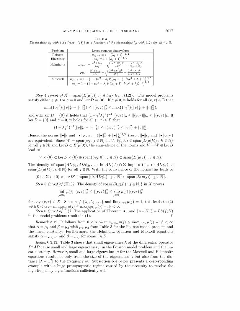
Table 3Eigenvalues \mu j with (16) (resp., (18)) as a function of the eigenvalues \lambda j with (12) for all j \in \BbbN .

Problem Least-squares eigenvalues

Poisson \mu 2j - 1 = 1 - (\lambda j + 1) - 1/2

Elasticity \mu 2j = 1 + (\lambda j + 1) - 1/2

Helmholtz \mu 2j - 1 =\omega 4+2\lambda j

2\lambda j -

\sqrt{} (\omega 4+2\lambda j)2

4\lambda 2j

- (\omega 2 - \lambda j)2

(\lambda j+1)\lambda j

\mu 2j =\omega 4+2\lambda j

2\lambda j+

\sqrt{} (\omega 4+2\lambda j)2

4\lambda 2j

- (\omega 2 - \lambda j)2

(\lambda j+1)\lambda j

Maxwell \mu 2j - 1 = 1 - \bigl( 1 - (\omega 2 - \lambda j)

2(\lambda j + 1) - 1(\omega 4 + \lambda j) - 1

\bigr) 1/2\mu 2j = 1 -

\bigl( 1 + (\omega 2 - \lambda j)

2(\lambda j + 1) - 1(\omega 4 + \lambda j) - 1

\bigr) 1/2Step 4 (proof of X = span\{ E(\mu (j)) : j \in \BbbN 0\} from (H2)). The model problems

satisfy either \gamma \not = 0 or \gamma = 0 and kerD = \{ 0\} . If \gamma \not = 0, it holds for all (v, \tau ) \in \Sigma that

min\{ 1, \gamma 2\} (\| v\| 2V + \| \tau \| 2\Sigma ) \leq \| (v, \tau )\| 2b \leq max\{ 1, \gamma 2\} (\| v\| 2V + \| \tau \| 2\Sigma ),

and with kerD = \{ 0\} it holds that (1+ \gamma 2\lambda - 11 ) - 1\| (v, \tau )\| b \leq \| (v, \tau )\| b0 \leq \| (v, \tau )\| b. If

kerD = \{ 0\} and \gamma = 0, it holds for all (v, \tau ) \in \Sigma that

(1 + \lambda - 11 ) - 1(\| v\| 2V + \| \tau \| 2\Sigma ) \leq \| (v, \tau )\| 2b \leq \| v\| 2V + \| \tau \| 2\Sigma .

Hence, the norms \| \bullet \| b and \| \bullet \| V\times \Sigma := (\| \bullet \| 2V + \| \bullet \| 2\Sigma )1/2 (resp., \| \bullet \| b0 and \| \bullet \| V\times \Sigma )

are equivalent. Since W = span\{ \psi j : j \in \BbbN \} in V , (\psi j , 0) \in span\{ E(\mu (k)) : k \in \BbbN \} for all j \in \BbbN , and kerD \subset E(\mu (0)), the equivalence of the norms and V =W \oplus kerDlead to

V \times \{ 0\} \subset kerD \times \{ 0\} \oplus span\{ (\psi j , 0) : j \in \BbbN \} \subset span\{ E(\mu (j)) : j \in \BbbN \} .

The density of span\{ AD\psi 1, AD\psi 2, . . . \} in AD(V ) \cap \Sigma implies that (0, AD\psi j) \in span\{ E(\mu (k)) : k \in \BbbN \} for all j \in \BbbN . With the equivalence of the norms this leads to

\{ 0\} \times \Sigma \subset \{ 0\} \times kerD\ast \oplus span\{ (0, AD\psi j) : j \in \BbbN \} \subset span\{ E(\mu (j)) : j \in \BbbN \} .

Step 5 (proof of (H1)). The density of span\{ E(\mu (j)) : j \in \BbbN 0\} in X proves

infj\in \BbbN 0

\mu (j)\| (v, \tau )\| 2b \leq \| (v, \tau )\| 2a \leq supj\in \BbbN 0

\mu (j)\| (v, \tau )\| 2b

for any (v, \tau ) \in X. Since \gamma /\in \{ \lambda 1, \lambda 2, . . . \} and limj\rightarrow \infty \mu (j) = 1, this leads to (2)with 0 < \alpha := minj\in \BbbN 0

\mu (j) \leq maxj\in \BbbN 0\mu (j) =: \beta <\infty .

Step 6 (proof of (1)). The application of Theorem 3.1 and \| u - U\| 2a = LS(f ;U)in the model problems results in (1).

Remark 3.12. It follows from 0 < \alpha := minj\in \BbbN 0 \mu (j) \leq maxj\in \BbbN 0 \mu (j) =: \beta < \infty that \alpha = \mu 1 and \beta = \mu 2 with \mu 1, \mu 2 from Table 3 for the Poisson model problem andthe linear elasticity. Furthermore, the Helmholtz equation and Maxwell equationssatisfy \alpha = \mu 2j - 1 and \beta = \mu 2j for some j \in \BbbN .

Remark 3.13. Table 3 shows that small eigenvalues \lambda of the differential operatorD\ast AD cause small and large eigenvalues \mu in the Poisson model problem and the lin-ear elasticity. However, small and large eigenvalues \mu for the Maxwell and Helmholtzequations result not only from the size of the eigenvalues \lambda but also from the dis-tance | \lambda - \omega 2| to the frequency \omega . Subsection 5.4 below presents a correspondingexample with a huge preasymptotic regime caused by the necessity to resolve thehigh-frequency eigenfunctions sufficiently well.

2018 CARSTEN CARSTENSEN AND JOHANNES STORN

Remark 3.14. The detailed analysis behind Table 3 is performed for four modelproblems but can be extended to other norms and bilinear forms exemplified for thealternative choice

b0(u, \sigma ; v, \tau ) = (A1/2Du,A1/2Dv)L2(\Omega ) + (A - 1/2\sigma ,A - 1/2\tau )L2(\Omega ) + (D\ast \sigma ,D\ast \tau )L2(\Omega )

for all (u, \sigma ), (v, \tau ) \in X for the Helmholtz equation in Table 3 and the \omega -independentnorm \| \bullet \| b0 induced by b0(\bullet , \bullet ). The Helmholtz equation admits the eigenvalues \mu 0 = 1and \mu j displayed for all j \in \BbbN in Table 3 of the eigenvalue problem

\forall (v, \tau ) \in X a(\phi j ; v, \tau ) = \mu jb0(\phi j ; v, \tau ).(18)

This follows analogously from the proof of Theorem 3.10, and so details are providedin section SM1 of the supplementary material.

3.3. The Poisson model problem with \bfitH 1-conforming compatible con-straint. The following FOSLS method for the Poisson model problem [11, 13] isbased on H1 conforming ansatz functions and adds the constraint curl p = 0 to theproblem in subsection 2.1. This ansatz leads to the norms

\| (v, \tau )\| 2a := \| \tau - \nabla v\| 2L2(\Omega ) + \| div \tau \| 2L2(\Omega ) + \| curl \tau \| 2L2(\Omega ),(19a)

\| (v, \tau )\| 2b := \| \nabla v\| 2L2(\Omega ) + \| \tau \| 2L2(\Omega ) + \| div \tau \| 2L2(\Omega ) + \| curl \tau \| 2L2(\Omega )(19b)

for all (v, \tau ) \in X := H10 (\Omega )\times (H(div,\Omega )\cap H(curl,\Omega )) with associated scalar product

a(\bullet , \bullet ) to \| \bullet \| a and b(\bullet , \bullet ) to \| \bullet \| b.Theorem 3.15. (a) The eigenvalue problem (16) has the eigenpairs (\mu j , \phi j) \in

\BbbR \times X, j \in \BbbN , from (15) for the Poisson model problem, and \mu 0 = 1 has the eigenspace\phi 0 \in \{ \tau \in H(div,\Omega ) \cap H(curl,\Omega ) : div \tau = 0\} .

(b) The model problem (19) satisfies (H1)--(H3) and (1).

Proof. Let (\lambda j , \psi j) \in \BbbR \times H10 (\Omega ), j \in \BbbN , denote the eigenpairs of the - \Delta operator.

The spectral representation of H10 (\Omega ) functions and the orthogonal split of Lemma 3.9

lead, for any (u, \sigma ) and (v, \tau ) in X, to coefficients uj , vj , \sigma j , \tau j \in \BbbR for j \in \BbbN and zero-divergence functions \sigma 0, \tau 0 \in H(div,\Omega ) \cap H(curl,\Omega ) with

u =\sum j\in \BbbN

uj\psi j , v =\sum j\in \BbbN

vj\psi j , \sigma = \sigma 0 +\sum j\in \BbbN

\sigma j\nabla \psi j , and \tau = \tau 0 +\sum j\in \BbbN

\tau j\nabla \psi j .

As in the proof of Theorem 3.10, this representation results in

a(u, \sigma ; v, \tau ) =\sum j\in \BbbN

\biggl( uj\xi j

\biggr) \cdot \biggl( \lambda j - \lambda j - \lambda j \lambda j + \lambda 2j

\biggr) \biggl( vj\vargamma j

\biggr) + (\sigma 0, \tau 0)L2(\Omega ) + (curl\sigma 0, curl \tau 0)L2(\Omega ),

b(u, \sigma ; v, \tau ) =\sum j\in \BbbN

\biggl( uj\xi j

\biggr) \cdot \biggl( \lambda j 00 \lambda j + \lambda 2j

\biggr) \biggl( vj\vargamma j

\biggr) + (\sigma 0, \tau 0)L2(\Omega ) + (curl\sigma 0, curl \tau 0)L2(\Omega ).

The remaining details of the proofs of (a) and (b) follow those in Theorems 3.10and 3.11 and are omitted for brevity.

4. Improved GUB. This section aims at the computation of a guaranteed up-per bound (GUB) for the model problems that capture the convergence of LS(f ;U)/\| u - U\| 2X to one.

ASYMPTOTIC EXACTNESS OF LS RESIDUALS 2019

4.1. A lower bound for the coercivity constant. Estimate (8) indicatesthat the coercivity constant on the a-orthogonal complement X(\scrT )\bot := \{ v \in X :\forall W \in X(\scrT ), a(v,W ) = 0\} of X(\scrT ) in X with \scrT \in \BbbT

\alpha \leq \alpha (\scrT ) := infv\in X(\scrT )\bot \setminus \{ 0\}

a(v, v)

\| v\| 2b(20)

converges to one as the mesh size tends to zeros. This constant improves the GUBfor the exact and discrete LSFEM solution u and U to

\| u - U\| 2b \leq \alpha (\scrT ) - 1\| u - U\| 2a \leq \alpha - 1\| u - U\| 2a.

The aim is the approximation of \alpha (\scrT ) - 1 from above by a constant C(\scrT ). The fol-lowing ansatz requires the smallest discrete eigenvalues \mu 1(\scrT ) \leq \cdot \cdot \cdot \leq \mu n(\scrT ) fora fixed n \leq dimX(\scrT ) with normed eigenfunctions \Phi 1, . . . ,\Phi n \in X(\scrT ), that is,\| \Phi 1\| b = \cdot \cdot \cdot = \| \Phi n\| b = 1 and

\forall j = 1, . . . , n \forall W \in X(\scrT ) a(\Phi j ,W ) = \mu j(\scrT ) b(\Phi j ,W ).(21)

Furthermore, let \mu 1 \leq \cdot \cdot \cdot \leq \mu n+1 be the smallest exact least-squares eigenvalues witheigenfunctions \phi 1, . . . , \phi n+1 such that b(\phi j , \phi k) = \delta jk for all j, k = 1, . . . , n+ 1, and

\forall w \in X a(\phi j , w) = \mu j b(\phi j , w).(22)

It follows from (H2) that 0 < \mu 1 and \{ \mu 1, . . . , \mu n+1\} \subset \{ \mu (j) : j \in \BbbN \} . The compari-son of exact and discrete eigenvalue clusters in \{ \mu 1, . . . , \mu n\} and \{ \mu 1(\scrT ), . . . , \mu n(\scrT )\} is the basic idea in the computation of C(\scrT ) \geq \alpha (\scrT ) - 1. Therefore, define for anycompact interval [\alpha \prime , \beta \prime ] \subset \BbbR the spaces

E(\alpha \prime , \beta \prime ) := span\{ E(\mu (j)) : j \in \BbbN 0, \alpha \prime \leq \mu (j) \leq \beta \prime \} \subset X,

E(\alpha \prime , \beta \prime , \scrT ) := span\{ \Phi j : j \in \{ 1, . . . , n\} , \alpha \prime \leq \mu j(\scrT ) \leq \beta \prime \} \subset X(\scrT ),

and let [\alpha 1, \beta 1], . . . , [\alpha m, \beta m] be intervals which satisfy the following hypothesis.(H4) Let [\alpha 1, \beta 1], . . . , [\alpha m, \beta m] be pairwise disjoint compact intervals with m \leq n

and 0 < \alpha 1 \leq \alpha \leq \beta 1 < \alpha 2 \leq \beta 2 < \cdot \cdot \cdot \leq \beta m < \alpha m+1, which satisfy, for all\ell = 1, . . . ,m,

dimE(\alpha \ell , \beta \ell ) = dimE(\alpha \ell , \beta \ell , \scrT ) and X = E(\alpha 1, \beta \ell )\oplus E(\alpha \ell +1, \beta ).

The intervals from (H4) lead to

C(\scrT ) := \alpha - 1m+1

\Biggl( 1 +

m\sum k=1

\alpha k+1\alpha m+1 - \alpha k

\alpha k\beta k

\beta k - \alpha k

\alpha k+1 - \alpha k

\Biggr) .(23)

Theorem 4.1. Suppose (H1)--(H4); then X(\scrT )\bot from (8) and C(\scrT ) satisfy

\forall v \in X(\scrT )\bot \| v\| 2b \leq C(\scrT )\| v\| 2a.

Remark 4.2. Suppose (H1)--(H4) and \alpha \ell = \mu (\ell ) for all \ell = 1, . . . ,m + 1 withthe smallest pairwise distinct eigenvalues \mu (1), \mu (2), . . . , \mu (m + 1) of (3). A smalleigenvalue error \delta := max\ell =1,...,m(\beta \ell - \mu (\ell )) of the discrete space guarantees

\alpha (\scrT ) - 1 \leq C(\scrT ) = \mu (m+ 1) - 1 +O(\delta ).

2020 CARSTEN CARSTENSEN AND JOHANNES STORN

Suppose the eigenvalue error is of the form \delta = O(hsmax) for some rate s > 0 and themaximal mesh-size hmax in \scrT . With a constant C(m), which depends in particularon m, (1) implies

\| u - U\| 2b/\| u - U\| 2a \leq \alpha (\scrT ) - 1 \leq C(\scrT ) \leq \mu (m+ 1) - 1 + C(m)hsmax.(24)

Proof of Theorem 4.1. Step 1 (decomposition of v \in X(\scrT )\bot ). Given any v \in X(\scrT )\bot \setminus \{ 0\} , (H2) implies X = E(\alpha 1, \beta 1) \oplus \cdot \cdot \cdot \oplus E(\alpha m, \beta m) \oplus E(\alpha m+1, \beta ) with\beta m+1 := \beta from (2) and so the existence of v1, . . . , vm+1 \in X with vj \in E(\alpha j , \beta j) for

all j = 1, . . . ,m+ 1 and v =\sum m+1

j=1 vj . The pairwise orthogonality of the eigenspaces(6) implies that a(vj , vk) = 0 = b(vj , vk) for all j, k = 1, . . . ,m+ 1 with j \not = k.

Step 2 (existence of Vj \in E(\alpha 1, \beta j , \scrT ) with vj - Vj \in E(\alpha j+1, \beta )). Let j \in \{ 1, . . . ,m\} and p = dimE(\alpha 1, \beta j), so that \phi 1, . . . , \phi p \in X form a basis of E(\alpha 1, \beta j).Since dimE(\alpha 1, \beta j) = dimE(\alpha 1, \beta j , \scrT ), there exists a basis \Phi 1, . . . ,\Phi p \in X(\scrT ) ofE(\alpha 1, \beta j , \scrT ). It holds that X(\scrT ) \subset X = E(\alpha 1, \beta j)\oplus E(\alpha j+1, \beta ). Consequently, thereexists a p\times p matrix B = (Bk\ell )k,\ell =1,...,p \in \BbbR p\times p with

\forall k = 1, . . . , p \Phi k - p\sum

\ell =1

Bk\ell \phi \ell \in E(\alpha j+1, \beta ).

To prove that B is invertible, let \xi = (\xi 1, . . . , \xi p) \in \BbbR p with B\xi = 0. In other words,\sum pk=1 \xi kBk\ell = 0 for all \ell = 1, . . . , p. Define

W := \xi 1\Phi 1 + \cdot \cdot \cdot + \xi p\Phi p \in E(\alpha 1, \beta j , \scrT ).

If \xi \not = 0, W \in E(\alpha 1, \beta j , \scrT ) \setminus \{ 0\} satisfies a(W,W )/b(W,W ) \leq \beta j . Furthermore, since

p\sum k=1

\xi k

p\sum \ell =1

Bk\ell \phi \ell =

p\sum \ell =1

\biggl( p\sum k=1

\xi kBk\ell

\biggr) \phi \ell = 0,

it holds that

W =W - p\sum

k=1

\xi k

p\sum \ell =1

Bk\ell \phi \ell =

p\sum k=1

\xi k

\biggl( \Phi k -

p\sum \ell =1

Bk\ell \phi \ell

\biggr) \in E(\alpha j+1, \beta ).

This implies \alpha j+1 \leq a(W,W )/b(W,W ) and contradicts \beta j < \alpha j+1. Therefore, W = 0and (\xi 1, . . . , \xi p) = 0. This proves that B is invertible. Thus, there exist coefficientsb\ell 1, . . . , b\ell p \in \BbbR for all \ell = 1, . . . , p with

\phi \ell - p\sum

k=1

b\ell k\Phi k \in E(\alpha j+1, \beta ).

This implies for vj \in span\{ \phi 1, . . . , \phi p\} the existence of Vj \in span\{ \Phi 1, . . . ,\Phi p\} with

vj - Vj \in E(\alpha j+1, \beta ) and Vj \in E(\alpha 1, \beta j , \scrT ).(25)

Step 3 (upper bound for \| Vj\| 2b). It follows from E(\alpha 1, \beta j) \bot a E(\alpha j+1, \beta ) andE(\alpha 1, \beta j) \bot b E(\alpha j+1, \beta ) that for Vj from Step 2 the Pythagoras theorem, \| vj\| 2a =\| Vj\| 2a - \| vj - Vj\| 2a and \| vj - Vj\| 2b = \| Vj\| 2b - \| vj\| 2b , holds. Since Vj \in E(\alpha 1, \beta j , \scrT ), itholds that \| Vj\| 2a \leq \beta j\| Vj\| 2b . Moreover, vj - Vj \in E(\alpha j+1, \beta ) implies \alpha j+1\| vj - Vj\| 2b \leq \| vj - Vj\| 2a; vj \in E(\alpha j , \beta j) induces \alpha j\| vj\| 2b \leq \| vj\| 2a. This leads to

\alpha j\| vj\| 2b \leq \| vj\| 2a = \| Vj\| 2a - \| vj - Vj\| 2a \leq \beta j\| Vj\| 2b - \alpha j+1(\| Vj\| 2b - \| vj\| 2b).

ASYMPTOTIC EXACTNESS OF LS RESIDUALS 2021

Consequently,

\| Vj\| 2b \leq \alpha j+1 - \alpha j

\alpha j+1 - \beta j\| vj\| 2b .(26)

Step 4 (upper bound for \| vj\| 2a). Case 1. Let vj \not = 0. This step utilizes a(vj , vj - Vj) = 0 = a(v, Vj) and a Cauchy--Schwarz inequality to deduce

\| vj\| 2a = a(v, vj) = a(v, vj - Vj) = a(v - vj , vj - Vj) \leq \| v - vj\| a\| vj - Vj\| a.

The combination with the Pythagoras theorem, \| v - vj\| 2a = \| v\| 2a - \| vj\| 2a and \| vj - Vj\| 2a = \| Vj\| 2a - \| vj\| 2a, leads to \| v\| 2a\| vj\| 2a + \| vj\| 2a\| Vj\| 2a \leq \| v\| 2a\| Vj\| 2a. Given vj \not = 0,it follows from vj - Vj \in E(\alpha j+1, \beta ) and E(\alpha j , \beta j)\cap E(\alpha j+1, \beta ) = \{ 0\} from (25) thatVj \not = 0. Consequently, the division of the previous estimate by \| v\| 2a\| vj\| 2a\| Vj\| 2a \not = 0results in

\| v\| - 2a + \| Vj\| - 2

a \leq \| vj\| - 2a .(27)

Since Vj \in E(\alpha j , \beta j , \scrT ) and vj \in E(\alpha j , \beta j) fulfill \beta - 1j \| Vj\| - 2

b \leq \| Vj\| - 2a and \| vj\| - 2

a \leq \alpha - 1j \| vj\| - 2

b , (26) leads in (27) to

\| vj\| 2b \leq \biggl(

1

\alpha j - \alpha j+1 - \beta j\beta j(\alpha j+1 - \alpha j)

\biggr) \| v\| 2a.(28)

Case 2. The estimate (28) is trivial for vj = 0.Step 5 (lower bound for \| v\| 2a). The estimate \alpha j\| vj\| 2b \leq \| vj\| 2a for all j =

1, . . . ,m+ 1 and the pairwise a- and b-orthogonality of v1, . . . , vm+1 prove

m\sum j=1

\alpha j\| vj\| 2b + \alpha m+1

\biggl( \| v\| 2b -

m\sum j=1

\| vj\| 2b\biggr)

\leq m+1\sum j=1

\| vj\| 2a = \| v\| 2a.(29)

Since \alpha j - \alpha m+1 < 0, the lower bound decreases monotonically in \| vj\| 2b for eachj = 1, . . . ,m and fixed \| v\| 2b . Hence, the substitution of (28) into (29) leads to

\alpha m+1\| v\| 2b \leq \| v\| 2a +m\sum j=1

(\alpha m+1 - \alpha j)

\biggl( 1

\alpha j - \alpha j+1 - \beta j\beta j(\alpha j+1 - \alpha j)

\biggr) \| v\| 2a

=

\left( 1 +

m\sum j=1

\alpha j+1\alpha m+1 - \alpha j

\alpha j\beta j

\beta j - \alpha j

\alpha j+1 - \alpha j

\right) \| v\| 2a.

4.2. Numerical realization. The application of Theorem 4.1 for the modelproblems runs a three-stage algorithm.

Stage 1. Compute N + 1 lower bounds 0 < \mu low1 \leq \cdot \cdot \cdot \leq \mu low

N+1 for the smallest

continuous eigenvalues in (16) (resp., (18)), i.e, \mu lowj \leq \mu j for j = 1, . . . , N + 1.

This computation is independent of the current triangulation and done offline. Thenumerical experiments in this paper adopt [1, 12] as detailed in section 5.

Stage 2. Given a triangulation \scrT \in \BbbT , compute upper bounds for the smallestdiscrete least-squares eigenvalues 0 < \mu 1(\scrT ) \leq \cdot \cdot \cdot \leq \mu N (\scrT ) with linear independenteigenfunctions \Phi 1, . . . ,\Phi N \in X(\scrT ) \setminus \{ 0\} such that

\forall \ell = 1, . . . , N \forall W \in X(\scrT ) a(\Phi \ell ,W ) = \mu \ell (\scrT )b(\Phi ,W ).(30)

2022 CARSTEN CARSTENSEN AND JOHANNES STORN

This leads to \mu up1 (\scrT ) \leq \cdot \cdot \cdot \leq \mu up

N (\scrT ) with \mu \ell (\scrT ) \leq \mu up\ell (\scrT ) for all \ell = 1, . . . , N .

The MATLAB function eigs (with standard parameters) solves (30) in section 5 andachieves \mu up

\ell (\scrT ) = \mu \ell (\scrT ) for all \ell = 1, . . . , N .Stage 3. Given the lower and upper eigenvalue bounds from Stages 1 and 2,

compute C(\scrT ) for all n = 0, . . . , N via the subsequent routine(i) set \alpha 1 := \mu low

1 and m := 0;(ii) for k = 1, . . . , n,

if \mu upk (\scrT ) < \mu low

k+1 then set m := m+ 1, \beta m := \mu upk (\scrT ), \alpha m+1 := \mu low

k+1;(iii) apply the formula (23);

Output: The minimum C(\scrT ) of the values from (iii) for n = 0, . . . , N

Proposition 4.3. The three-stage algorithm leads to C(\scrT ) in Theorem 4.1.

Proof. It suffices to show that the values \alpha 1, . . . , \alpha m+1 and \beta 1, . . . , \beta m from (i) and(ii) in Stage 3 with n = 0, . . . , N satisfy (H4) for all \ell = 1, . . . ,m. Then Theorem 4.1applies to all n = 0, . . . , N and results in the GUB.

Step 1 (proof of 0 < \alpha 1 \leq \alpha \leq \beta 1 < \alpha 2 \leq \beta 2 < \cdot \cdot \cdot \leq \beta m < \alpha m+1). For allj = 1, . . . , n, the Rayleigh--Ritz principle leads to

\mu lowj \leq \mu j = min

Xj\subset XdimXj=j

maxv\in Xj

\| v\| b=1

a(v, v) \leq \mu j(\scrT ) = minXj(\scrT )\subset X(\scrT )dimXj(\scrT )=j

maxV \in Xj(\scrT )\| V \| b=1

a(V, V ) \leq \mu upj (\scrT ).

This proves 0 < \alpha 1 = \mu low1 \leq \mu 1 = \alpha \leq \mu up

1 (\scrT ) = \beta 1. Moreover, for all \ell = 1, . . . ,mthere exists a k \in \{ 1, . . . , n\} such that \beta \ell = \mu up

k (\scrT ) < \mu lowk+1 = \alpha \ell +1. If \ell < m, it also

holds that \alpha \ell +1 = \mu lowk+1 \leq \mu up

k+1(\scrT ) \leq \beta \ell +1.Step 2 (proof of dimE(\alpha \ell , \beta \ell ) = dimE(\alpha \ell , \beta \ell , \scrT )). Given an interval [\alpha \ell , \beta \ell ]

with \ell = 1, . . . ,m, let \ell 1 \in \{ 1, . . . , n\} be the smallest index with \alpha \ell = \mu low\ell 1

and\ell 2 \in \{ \ell 1, . . . , n\} the biggest index with \beta \ell = \mu up

\ell 2(\scrT ). Then

\alpha \ell = \mu low\ell 1 \leq \mu \ell 1 \leq \mu \ell 1+1 \leq \cdot \cdot \cdot \leq \mu \ell 2 \leq \mu up

\ell 2(\scrT ) = \beta \ell

implies \ell 2 - \ell 1 + 1 \leq dimE(\alpha \ell , \beta \ell ). If \ell 2 - \ell 1 + 1 < dimE(\alpha \ell , \beta \ell ), there existsan eigenpair (\mu , \phi ) \in [\alpha \ell , \beta \ell ] \times X \setminus \{ 0\} with a(\phi ,w) = \mu b(\phi ,w) for all w \in X andb(\phi , \phi k) = 0 for all k = 1, . . . , n + 1. The eigenvalue \mu is strictly smaller than\mu \ell 2+1. This contradicts the assumption that \mu 1, . . . , \mu n+1 are the smallest eigenvalues.Therefore, dimE(\alpha \ell , \beta \ell ) = \ell 2 - \ell 1 + 1. Similar arguments lead to dimE(\alpha \ell , \beta \ell , \scrT ) =\ell 2 - \ell 1 + 1.

Step 3 (proof of X = E(\alpha 1, \beta \ell ) \oplus E(\alpha \ell +1, \beta )). For all \ell = 1, . . . ,m there existsk \in \{ 1, . . . , n\} with \mu k \leq \mu up

k (\scrT ) = \beta \ell < \alpha \ell +1 = \mu lowk+1 \leq \mu k+1. Let \phi j \in E(\mu (j)) with

j \in \BbbN . Since \mu 1, . . . , \mu n are the smallest eigenvalues with (22), it holds that either\mu (j) \leq \mu k or \mu k+1 \leq \mu (j). This reveals \phi j \in E(\alpha 1, \beta \ell ) or \phi j \in E(\alpha \ell +1, \beta ). Therefore,any eigenfunction belongs to E(\alpha 1, \beta \ell )\oplus E(\alpha \ell +1, \beta ). The density of the linear hull ofeigenfunctions in X from (H2) implies X = E(\alpha 1, \beta \ell )\oplus E(\alpha \ell +1, \beta ).

Remark 4.4. It follows from the Rayleigh--Ritz principle that \mu up1 (\scrT ), . . . , \mu up

N (\scrT )are upper bounds for the smallest discrete eigenvalues in (30) for any discrete space\^X(\scrT ) with X(\scrT ) \subset \^X(\scrT ). Thus, the GUB C(\scrT )LS(f ; \^U) holds for the solution \^Uto the LSFEM with any discrete space \^X(\scrT ) with X(\scrT ) \subset \^X(\scrT ). This enables thepossibility of applying (adaptive) hp-refinements.

5. Numerical experiments. This section underlines the theoretical results ofthis paper with numerical experiments for the Poisson model problem, the Helmholtzequation, and the Maxwell equations and exploits its efficiency.

ASYMPTOTIC EXACTNESS OF LS RESIDUALS 2023

101 102 103 104 105 106

0.6

0.8

1

ndof

102 103 104 105 106

0.6

0.8

1

ndof

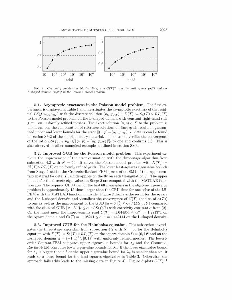
Fig. 2. Coercivity constant \alpha (dashed line) and C(\scrT ) - 1 on the unit square (left) and theL-shaped domain (right) in the Poisson model problem.

5.1. Asymptotic exactness in the Poisson model problem. The first ex-periment is displayed in Table 1 and investigates the asymptotic exactness of the resid-ual LS(f ;uC , pRT ) with the discrete solution (uC , pRT ) \in X(\scrT ) := S1

0(\scrT )\times RT0(\scrT )to the Poisson model problem on the L-shaped domain with constant right-hand sidef \equiv 1 on uniformly refined meshes. The exact solution (u, p) \in X to the problem isunknown, but the computation of reference solutions on finer grids results in guaran-teed upper and lower bounds for the error \| (u, p) - (uC , pRT )\| X ; details can be foundin section SM2 of the supplementary material. The outcome verifies the convergenceof the ratio LS(f ;uC , pRT )/\| (u, p) - (uC , pRT )\| 2X to one and confirms (1). This isalso observed in other numerical examples outlined in section SM3.

5.2. Improved GUB for the Poisson model problem. This experiment ex-ploits the improvement of the error estimation with the three-stage algorithm fromsubsection 4.2 with N = 60. It solves the Poisson model problem with X(\scrT ) :=S10(\scrT )\times RT0(\scrT ) on uniformly refined grids. The lower least-squares eigenvalue bounds

from Stage 1 utilize the Crouzeix--Raviart-FEM (see section SM4 of the supplemen-tary material for details), which applies on the fly on each triangulation \scrT . The upperbounds for the discrete eigenvalues in Stage 2 are computed with the MATLAB func-tion eigs. The required CPU time for the first 60 eigenvalues in the algebraic eigenvalueproblem is approximately 15 times larger than the CPU time for one solve of the LS-FEM with the MATLAB function mldivide. Figure 2 displays the result for the squareand the L-shaped domain and visualizes the convergence of C(\scrT ) (and so of \alpha (\scrT ))to one as well as the improvement of the GUB \| u - U\| 2X \leq C(\scrT )LS(f ;U) comparedwith the classical GUB \| u - U\| 2X \leq \alpha - 1LS(f ;U) with coercivity constant \alpha from (2).On the finest mesh the improvements read C(\scrT ) = 1.044854 \leq \alpha - 1 = 1.281371 onthe square domain and C(\scrT ) = 1.108241 \leq \alpha - 1 = 1.442114 on the L-shaped domain.

5.3. Improved GUB for the Helmholtz equation. This subsection investi-gates the three-stage algorithm from subsection 4.2 with N = 60 for the Helmholtzequation with X(\scrT ) := S1

0(\scrT )\times RT0(\scrT ) on the square domain \Omega = (0, 1)2 and on theL-shaped domain \Omega = ( - 1, 1)2 \setminus [0, 1)2 with uniformly refined meshes. The lowest-order Courant-FEM computes upper eigenvalue bounds for \lambda k and the Crouzeix--Raviart-FEM computes lower eigenvalue bounds for \lambda k. If the lower eigenvalue boundfor \lambda k is bigger than \omega 2 or the upper eigenvalue bound for \lambda k is smaller than \omega 2, itleads to a lower bound for the least-squares eigenvalue in Table 3. Otherwise, theapproach fails (this leads to the missing data in Figure 4). Figure 3 plots C(\scrT ) - 1

2024 CARSTEN CARSTENSEN AND JOHANNES STORN

101 102 103 104 105 106

0

0.5

1

ndof

ω = 1

ω = 2

102 103 104 105 106

0

0.5

1

ndof

ω = 1

ω = 2

Fig. 3. Coercivity constant \alpha (dashed line) and C(\scrT ) - 1 on the unit square (left) and theL-shaped domain (right) in the Helmholtz equation.

for \omega = 1 and \omega = 2. It indicates the convergence of C(\scrT ) - 1 (and so of \alpha (\scrT )) toone. The reliability constant C(\scrT ) improves the classical reliability constant \alpha - 1 onthe finest grid as follows: C(\scrT ) = 1.093083 \leq \alpha - 1 = 1.708149 on the square do-main with \omega = 1, C(\scrT ) = 1.253660 \leq \alpha - 1 = 4.256367 on the square domain with\omega = 2, C(\scrT ) = 1.237410 \leq \alpha - 1 = 2.290786 on the L-shaped domain with \omega = 1,C(\scrT ) = 1.758341 \leq \alpha - 1 = 11.521603 on the L-shaped domain with \omega = 2.

5.4. Improved GUB for the Helmholtz equation with large frequen-cies. Table 4 compares the reliability constant \alpha - 1 (computed with the Dirichleteigenvalues of - \Delta from [21] and [17]) with the reliability constant C(\scrT ) (computedwith the three-stage algorithm from subsection 4.2) for the Helmholtz equation ofsubsection 5.3 with frequencies \omega = 0, . . . , 10. For frequencies \omega \geq 7 the compu-tation leads to C(\scrT ) close to \alpha - 1. In other words, the improvement of the GUBwith the three-stage algorithm was negligible. To study the efficiency of the GUBC(\scrT )LS(f ;U), Figure 4 and Table 5 compare the residual and the exact error ofthe LSFEM for the Helmholtz equation on the unit square with \omega = 4 and knownsolution (sin(\pi x) sin(\pi y),\nabla sin(\pi x) sin(\pi y)) as well as with \omega = 7 and known solu-tion (sin(2\pi x) sin(\pi y),\nabla sin(2\pi x) sin(\pi y)). The experiment indicates that the GUB\alpha - 1LS(f ;U) is indeed an accurate upper bound in the preasymptotic regime andcannot be improved by C(\scrT ). However, for finer triangulations and small frequen-cies such as \omega = 4, the GUB C(\scrT )LS(f ;U) captures the fast decay of the error andresults in an improvement by several orders of magnitude and so justifies the higherCPU time as discussed in subsection 5.7. For large frequencies \omega \geq 7, the FEM doesnot resolve the highly oscillating eigenfunctions in the computational domain of thisexperiment. This provides numerical evidence for an efficient error control despite thefact that the constant is far away from one in the preasymptotic regime. The limitedmemory of the computer does not allow us to determine the constant C(\scrT ) on finergrids than the nine times uniformly refined mesh \scrT 9, and so C(\scrT 9) is applied to finermeshes as well with reduced efficiency.

5.5. Improved GUB for the Maxwell equations. The three-stage algorithmfrom subsection 4.2 is run with N = 20 to the Maxwell LSFEM withX(\scrT ) = \scrN 0

0 (\scrT )\times \scrN 0(\scrT ) on the cube domain \Omega = (0, 1)3 and the Fichera corner domain \Omega = ( - 1, 1)3 \setminus [0, 1)3. The lower eigenvalue bounds in Stage 1 are taken from the exact Maxwelleigenvalues \lambda j on the cube domain from [16]. The upper and lower eigenvalue boundsfor \lambda j on the Fichera corner domain from [1] lead with the identities in Table 3 to

ASYMPTOTIC EXACTNESS OF LS RESIDUALS 2025

Table 4Reliability constants C(\scrT ) and \alpha - 1 in the Helmholtz equation on the uniformly refined unit

square with ndof = 1048577, hmax = 2 - 15/2 (left) and the L-shaped domain with ndof = 786433,hmax = 2 - 13/2 (right).

\omega C(\scrT ) \alpha - 1

0 1.04485379 1.281370561 1.09308333 1.708148602 1.25365982 4.256368033 1.58732441 21.49980954 3.32921432 438.2197765 4.73101753 497.9038256 8.98796502 394.0840117 1010101.01 1041666.668 160.287234 1520.403829 90171.3255 128700.12910 558659.22 598802.395

\omega C(\scrT ) \alpha - 1

0 1.10824134 1.442114221 1.23740999 2.290785852 1.75834047 11.52160283 2.34866936 2607.018094 7.40823054 7198.387565 193.267713 1021.200116 1319.38306 2678.882377 1204819.28 1041666.678 151285.930 -9 125786.164 -10 609756.098 -

101 102 103 104 105 106 10710−5

10−1

103

ndof

101 102 103 104 105 106 10710−4

100

104

ndof

Fig. 4. Error \| u - U\| 2X ( ), residual LS(f ;U) ( ), GUB LS(f ;U)/\alpha ( ), and GUBC(\scrT )LS(f ;U) ( ) in the Helmholtz equation with \omega = 4 (left) and \omega = 7 (right).

Table 5Ieff(C(\scrT )) := C(\scrT )1/2LS(f ;U)1/2/\| u - U\| X and Ieff(\alpha ) := \alpha - 1/2LS(f ;U)1/2/\| u - U\| X .

\omega = 4 \omega = 7ndof Ieff(C(\scrT )) Ieff(\alpha ) Ieff(C(\scrT )) Ieff(\alpha )257 33.44 1.23 - 1.751025 1.60 1.29 - 1.244097 1.27 1.77 - 1.0616385 1.22 3.02 - 1.0265537 1.23 5.56 1.47 1.01262145 1.25 9.72 1.09 1.011048577 1.23 14.15 1.03 1.054194305 1.46 16.70 1.15 1.1716777217 1.53 17.60 1.54 1.56

lower eigenvalue bounds for the Fichera corner domain. Table 6 shows a preasymptoticregime with C(\scrT ) and \alpha - 1 close (C(\scrT ) = \alpha - 1 on the coarsest mesh) together withoutsignificant improvement of C(\scrT ). As hmax \ll 1 decreases, the values C(\scrT ) decreaseand lead to a smaller reliability constant.

5.6. Convergence speed. Remark 4.2 states that with a fixed number N ofapproximated eigenvalues the constant C(\scrT ) - 1 converges toward the inverse \mu - 1

N+1 oftheN+1 smallest least-squares eigenvalue \mu N+1 in (16) (resp., (18)). The convergencespeed depends on the convergence speed of the eigenvalue bounds toward the exact

2026 CARSTEN CARSTENSEN AND JOHANNES STORN

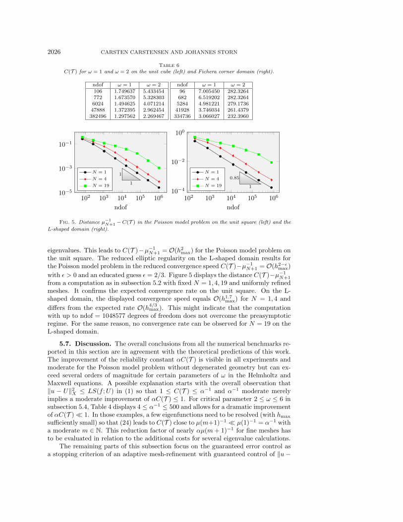
Table 6C(\scrT ) for \omega = 1 and \omega = 2 on the unit cube (left) and Fichera corner domain (right).

ndof \omega = 1 \omega = 2106 1.749637 5.433454772 1.673570 5.3283036024 1.494625 4.07121447888 1.372395 2.962454382496 1.297562 2.269467

ndof \omega = 1 \omega = 296 7.005450 282.3264682 6.519202 282.32645284 4.981221 279.173641928 3.746034 261.4379334736 3.066027 232.3960

102 103 104 105 10610−5

10−3

10−1

1

1

ndof

N = 1

N = 4

N = 19

102 103 104 105 10610−4

10−2

100

0.85

1

ndof

N = 1

N = 4

N = 19

Fig. 5. Distance \mu - 1N+1 - C(\scrT ) in the Poisson model problem on the unit square (left) and the

L-shaped domain (right).

eigenvalues. This leads to C(\scrT ) - \mu - 1N+1 = \scrO (h2max) for the Poisson model problem on

the unit square. The reduced elliptic regularity on the L-shaped domain results forthe Poisson model problem in the reduced convergence speed C(\scrT ) - \mu - 1

N+1 = \scrO (h2 - \epsilon max)

with \epsilon > 0 and an educated guess \epsilon = 2/3. Figure 5 displays the distance C(\scrT ) - \mu - 1N+1

from a computation as in subsection 5.2 with fixed N = 1, 4, 19 and uniformly refinedmeshes. It confirms the expected convergence rate on the unit square. On the L-shaped domain, the displayed convergence speed equals \scrO (h1.7max) for N = 1, 4 and

differs from the expected rate \scrO (h4/3max). This might indicate that the computation

with up to ndof = 1048577 degrees of freedom does not overcome the preasymptoticregime. For the same reason, no convergence rate can be observed for N = 19 on theL-shaped domain.

5.7. Discussion. The overall conclusions from all the numerical benchmarks re-ported in this section are in agreement with the theoretical predictions of this work.The improvement of the reliability constant \alpha C(\scrT ) is visible in all experiments andmoderate for the Poisson model problem without degenerated geometry but can ex-ceed several orders of magnitude for certain parameters of \omega in the Helmholtz andMaxwell equations. A possible explanation starts with the overall observation that\| u - U\| 2X \leq LS(f ;U) in (1) so that 1 \leq C(\scrT ) \leq \alpha - 1 and \alpha - 1 moderate merelyimplies a moderate improvement of \alpha C(\scrT ) \leq 1. For critical parameter 2 \leq \omega \leq 6 insubsection 5.4, Table 4 displays 4 \leq \alpha - 1 \leq 500 and allows for a dramatic improvementof \alpha C(\scrT ) \ll 1. In those examples, a few eigenfunctions need to be resolved (with hmax

sufficiently small) so that (24) leads to C(\scrT ) close to \mu (m+1) - 1 \ll \mu (1) - 1 = \alpha - 1 witha moderate m \in \BbbN . This reduction factor of nearly \alpha \mu (m+ 1) - 1 for fine meshes hasto be evaluated in relation to the additional costs for several eigenvalue calculations.

The remaining parts of this subsection focus on the guaranteed error control asa stopping criterion of an adaptive mesh-refinement with guaranteed control of \| u -

ASYMPTOTIC EXACTNESS OF LS RESIDUALS 2027

U\| X smaller than a given tolerance tol. Suppose that a fine triangulation \scrT satisfiesC(\scrT )LS(f ;U) \leq tol2 with ndof degrees of freedom in the discrete system. For asimplified comparison, suppose that the computational costs CPU are proportional tondof (for an optimal iterative solver despite the fact that our numerical examples runwith the direct MATLAB solver mldivide). Subsection 5.2 suggests that the adaptivealgorithm may stop with the triangulation \scrT , but requires extra costs of 15CPU forthe more expansive improved GUB; the final result is obtained with the costs 16CPU(online) with the application of the three-stage algorithm of subsection 4.2. In thepresent model situation, the usage of \alpha - 1LS(f ;U) implies further mesh-refinementsuntil the bound \alpha - 1LS(f ;U \prime ) \leq tol2 holds for a discrete solution U \prime with respectto a much finer mesh \scrT \prime with ndof\prime degrees of freedom. In the case of low-orderdiscretizations at hand and an optimal convergence rate 0.5 of the adaptive algorithmin 2D, one may expect \alpha ndof\prime = ndof/C(\scrT ). The computational costs of the discretesolutions with respect to \scrT \prime are larger than \alpha - 1C(\scrT ) - 1. Hence, if \alpha C(\scrT ) \leq 1/16, thethree-stage algorithm of subsection 4.2 appears less expensive in the computationalonline costs. This calculation leaves out the additional mesh-refinements requiredin the adaptive algorithm to compute \scrT \prime and therefore is very conservative. Thisdiscussion also ignores the fact that C( \v \scrT ) may be computed on a moderate mesh \v \scrT and may utilize C(\scrT ) \leq C( \v \scrT ) for all refinements \scrT .

The offline costs concern the eigenvalues of the domain, which are known insubsection 5.5 and are less laborious in subsections 5.2--5.4: the convergence rateO(h2smax) of the eigenvalue error is of higher order compared to O(hsmax) in the sourceproblem for s \leq 1 depending on the reduced elliptic regularity.

Based on this discussion, the three-stage algorithm of subsection 4.2 is advanta-geous in subsection 5.4 for 3 \leq \omega \leq 6 (and for higher \omega with much finer meshes). Asa rule of thumb, the proposed algorithm appears advantageous if 16\alpha \leq \mu (m+ 1) formoderate m and sufficiently small tolerances in guaranteed error control.

Acknowledgments. The work was written while the authors enjoyed the hospi-tality of the Hausdorff Research Institute of Mathematics in Bonn, Germany, duringthe Hausdorff Trimester Program ``Multiscale Problems: Algorithms, Numerical Anal-ysis and Computation"". The constructive suggestions of the anonymous referees ledto an improved revision and in particular to the addition of subsections 3.3 and 5.7.

REFERENCES

[1] G. R. Barrenechea, L. Boulton, and N. Boussa\"{\i}d, Local two-sided bounds for eigenvaluesof self-adjoint operators, Numer. Math., 135 (2017), pp. 953--986, https://doi.org/10.1007/s00211-016-0822-1.

[2] P. Bochev and M. Gunzburger, On least-squares finite element methods for the Poissonequation and their connection to the Dirichlet and Kelvin principles, SIAM J. Numer.Anal., 43 (2005), pp. 340--362, https://doi.org/10.1137/S003614290443353X.

[3] P. B. Bochev and M. D. Gunzburger, Least-Squares Finite Element Methods, Appl. Math.Sci. 166, Springer, New York, 2009, https://doi.org/10.1007/b13382.

[4] D. Boffi, F. Brezzi, and M. Fortin, Mixed Finite Element Methods and Applications,Springer Ser. Comput. Math. 44, Springer, Heidelberg, 2013, https://doi.org/10.1007/978-3-642-36519-5.

[5] D. Braess, Finite Elements. Theory, Fast Solvers, and Applications in Elasticity Theory, 3rded., Cambridge University Press, Cambridge, UK, 2007.

[6] J. H. Bramble, T. V. Kolev, and J. E. Pasciak, A least-squares approximation method forthe time-harmonic Maxwell equations, J. Numer. Math., 13 (2005), pp. 237--263, https://doi.org/10.1163/156939505775248347.

2028 CARSTEN CARSTENSEN AND JOHANNES STORN

[7] S. C. Brenner and L. R. Scott, The Mathematical Theory of Finite Element Methods,Texts Appl. Math. 15, 3rd ed., Springer, New York, 2008, https://doi.org/10.1007/978-0-387-75934-0.

[8] Z. Cai, V. Carey, J. Ku, and E.-J. Park, Asymptotically exact a posteriori error estimatorsfor first-order div least-squares methods in local and global L2 norm, Comput. Math. Appl.,70 (2015), pp. 648--659, https://doi.org/10.1016/j.camwa.2015.05.010.

[9] Z. Cai, J. Korsawe, and G. Starke, An adaptive least squares mixed finite element methodfor the stress-displacement formulation of linear elasticity, Numer. Methods Partial Dif-ferential Equations, 21 (2005), pp. 132--148, https://doi.org/10.1002/num.20029.

[10] Z. Cai, R. Lazarov, T. A. Manteuffel, and S. F. McCormick, First-order system leastsquares for second-order partial differential equations: Part I, SIAM J. Numer. Anal., 31(1994), pp. 1785--1799, https://doi.org/10.1137/0731091.

[11] Z. Cai, T. A. Manteuffel, and S. F. McCormick, First-order system least squares forsecond-order partial differential equations: Part II, SIAM J. Numer. Anal., 34 (1997),pp. 425--454, https://doi.org/10.1137/S0036142994266066.

[12] C. Carstensen and J. Gedicke, Guaranteed lower bounds for eigenvalues, Math. Comp., 83(2014), pp. 2605--2629, https://doi.org/10.1090/S0025-5718-2014-02833-0.

[13] C. L. Chang, Finite element approximation for grad-div type systems in the plane, SIAM J.Numer. Anal., 29 (1992), pp. 452--461, https://doi.org/10.1137/0729027.

[14] P. G. Ciarlet, Mathematical Elasticity. Vol. I. Three-Dimensional Elasticity, Stud. Math.Appl. 20, North--Holland, Amsterdam, 1988.

[15] P. G. Ciarlet and J.-L. Lions, eds., Handbook of Numerical Analysis. Vol. II. Finite ElementMethods. Part 1, North--Holland, Amsterdam, 1991.

[16] M. Costabel and M. Dauge, Maxwell Eigenmodes in Tensor Product Domains, https://perso.univ-rennes1.fr/monique.dauge/publis/CoDa06MaxTens2.pdf, 2006.

[17] D. Gallistl, Adaptive Finite Element Computation of Eigenvalues, doctoral dissertation,Humboldt-Universit\"at zu Berlin, Mathematisch-Naturwissenschaftliche Fakult\"at II, 2014,http://edoc.hu-berlin.de/docviews/abstract.php?id=40852.

[18] B.-N. Jiang and L. A. Povinelli, Optimal least-squares finite element method for ellipticproblems, Comput. Methods Appl. Mech. Engrg., 102 (1993), pp. 199--212, https://doi.org/10.1016/0045-7825(93)90108-A.

[19] P. Monk, Finite Element Methods for Maxwell's Equations, Numer. Math. Sci. Comput., Ox-ford University Press, New York, 2003, https://doi.org/10.1093/acprof:oso/9780198508885.001.0001.

[20] A. I. Pehlivanov, G. F. Carey, and R. D. Lazarov, Least-squares mixed finite elements forsecond-order elliptic problems, SIAM J. Numer. Anal., 31 (1994), pp. 1368--1377, https://doi.org/10.1137/0731071.

[21] L. N. Trefethen and T. Betcke, Computed eigenmodes of planar regions, in Recent Ad-vances in Differential Equations and Mathematical Physics, Contemp. Math. 412, AMS,Providence, RI, 2006, pp. 297--314, https://doi.org/10.1090/conm/412/07783.