atena program documentation part 8 user's manual for atena
TRANSCRIPT
Červenka Consulting, s.r.o Na Hrebenkach 55/2667 150 00 Prague Czech Republic Phone: +420 220 610 018 E-mail: [email protected] Web: http://www.cervenka.cz
ATENA Program Documentation Part 8 User’s Manual for ATENA-GiD Interface Written by Vladimír Červenka, Jan Červenka,
Zdeněk Janda, and Dobromil Pryl
Prague, October 6th, 2017

Ackowledgements:
The software was developed with partial support of Eurostars funding program.
The following models were developed with the financial support of TA ČR: CC3DNonLinCementitious2HPRFC, CC3DNonLinCementitious2FRC, CC3DNonLinCementitious2SHCC, CCModelGeneral, CCTransportMaterial
Trademarks:
ATENA is registered trademark of Vladimir Cervenka.
GiD is registered trademark of CIMNE of Barcelona, Spain.
Microsoft and Microsoft Windows are registered trademarks of Microsoft Corporation.
Other names may be trademarks of their respective owners.
Copyright © 2000-2017 Červenka Consulting, s.r.o.
ATENA Science - GiD - User´s Manual i
CONTENTS
1 INTRODUCTION............................................................................................................ 1
2 OVERVIEW .................................................................................................................. 3
2.1 Working with GiD .......................................................................................................................3
2.2 Limitations of ATENA-GiD Interface.....................................................................................3
3 GID INSTALLATION AND REGISTRATION .......................................................................... 5
3.1 GiD Network Floating Licenses..............................................................................................6
4 ATENA-GID INSTALLATION ......................................................................................... 7
4.1 Manual Installation of the ATENA-GiD Scripts.................................................................7
5 ATENA - SPECIFIC COMMANDS..................................................................................... 9
5.1 Problem Type ...............................................................................................................................9
5.2 Conditions .....................................................................................................................................9
5.3 Materials...................................................................................................................................... 24
5.3.1 Solid Concrete Material.....................................................................................................29
5.3.2 Shell Material .......................................................................................................................40
5.3.3 Beam Material .....................................................................................................................46
5.3.4 Reinforced Concrete...........................................................................................................49
5.3.5 1D Reinforcement Material ..............................................................................................50
5.3.6 Interface Material ...............................................................................................................56
5.3.7 Spring material....................................................................................................................61
5.3.8 The Material Function ......................................................................................................63
5.3.9 Material from file ................................................................................................................64
5.3.10 Dummy Material.................................................................................................................64
5.4 Interval Data - Loading History........................................................................................... 65
5.4.1 Fatigue...................................................................................................................................69
5.5 Problem Data ............................................................................................................................ 72
5.6 Units.............................................................................................................................................. 75
5.7 Finite Element Mesh ............................................................................................................... 76
5.7.1 Notes on Meshing...............................................................................................................76
ii
5.7.2 Finite Elements for ATENA................................................................................................ 77
5.8 ATENA Menu ..............................................................................................................................81
6 STATIC ANALYSIS .......................................................................................................83
7 CREEP ANALYSIS (AND SHRINKAGE) ..............................................................................85
7.1 Boundary Conditions and Load Cases Related Input .................................................86
7.2 Specific Creep Boundary Conditions ................................................................................87
7.3 Material Input Data ..................................................................................................................87
8 TRANSPORT ANALYSIS (MOISTURE AND HEAT)................................................................91
8.1 Material Input Data ..................................................................................................................91
8.1.1 Material CCTransport (CERHYD) .................................................................................... 91
8.1.2 Material Bazant_Xi_1994 (only included for backward compatibility of old models)................................................................................................................................................ 98
8.2 Other Settings Related to Transport Analysis................................................................99
8.3 Specific Transport Boundary Conditions...................................................................... 102
9 DYNAMIC ANALYSIS ................................................................................................ 105
9.1 Specific Dynamic Boundary Conditions ....................................................................... 107
10 POST-PROCESSING IN ATENA-GID ........................................................................... 111
11 USEFUL TIPS AND TRICKS......................................................................................... 119
11.1 Export IXT for ATENA 3D Pre-processor........................................................................ 119
12 EXAMPLE DATA FILES .............................................................................................. 121
13 CALCULATION OF ATENA IDENTIFICATION NUMBERS .................................................. 123
REFERENCES ................................................................................................................... 125
ATENA Science - GiD - User´s Manual 1
1 INTRODUCTION Program GiD can be used for the preparation of input data for ATENA analysis. The program GiD is a universal, adaptive and user-friendly graphical user interface for geometrical modelling and data input for all types of numerical simulation programs. It has been developed at CIMNE (The International Center for Numerical Methods in Engineering, http://www.cimne.upc.es) in Barcelona, Spain. When using GiD, for some graphic cards it may be necessary to switch off “graphical acceleration”.
Several scripts are created, which enables to interface GiD with ATENA. Selecting an appropriate problem type in the GiD environment activates these scripts:
Problem types are compatible with GiD ver.7.7.2b and newer, version 10 or 11 is recommended):
ATENA/Static, - static 2D and 3D analysis
ATENA/Creep, - creep 2D and 3D analysis
ATENA/Transport, - transport 2D and 3D analysis
ATENA/Dynamic - dynamic 2D and 3D analysis
These problem types make it possible to define a finite element model within GiD including specific data needed for ATENA analysis. ATENA Studio [5] can be launched directly from GiD, and the non-linear analysis can be performed. Visualization of ATENA results is also possible in GiD, but it can be done also in the Pre/Post-processor of ATENA 3D [3], which is a powerful ATENA postprocessor. However, this option is available only if ATENA Engineering is installed on your computer. The recommended post/processing environment is ATENA Studio [5].
The problem types with the label ATENA can be used with ATENA version newer than 5.0.0. These problem types support ATENA analysis with two- and three-dimensional models (including axi-symmetrical models). In addition it is possible to perform stress, creep, thermal (i.e. transport) and dynamic analyses.
A demo version of GiD is limited to 3000 elements (or 1010 nodes). It can be downloaded free of charge from http://www.gidhome.com/, or from our web pages www.cervenka.cz .
This document describes the way how GiD can be used to generate data for ATENA analysis. The emphasis is on ATENA-oriented commands. More details about the general use of GiD for the development of the geometric model can be found in the GiD documentation.

2
ATENA Science - GiD - User´s Manual 3
2 OVERVIEW
2.1 Working with GiD The procedure of data preparation for ATENA analysis with the help of GiD can be summarized in the following work sequence:
Select one of the problem types for ATENA.
Create a geometrical model.
Impose conditions such as boundary conditions and loading on the geometrical model.
Select material models, define parameters and assign them to the geometry.
Generate finite element mesh.
Change or assign supports and loading conditions to the mesh nodes (if necessary).
Change or assign materials to individual finite elements (if necessary).
Create loading history by defining interval data.
Execute finite element analysis with ATENA Studio or AtenaConsole.
Some of the above actions are general and not dependent on ATENA (geometry definition, finite element mesh), while the others are more or less specific for ATENA (material parameters, solution methods). This manual is focused on the later features.
The description of the general features of GiD (menu items View, Geometry, Utilities, etc.) can be found in the GiD documentation. There is an extensive online help available in GiD, which is accessible from the menu Help as well as some online tutorials. For example the information how to create geometry is not included in this manual, and can be found in the GiD menu Help | Contents | Geometry.
In the ATENA-specific dialogs (materials, conditions, etc.), help is also available with detailed description and additional information by clicking the right mouse click or the
help icon .
The practical aspects of the GiD use can be exercised on the examples described in Chapter 12. It is also recommended to go through the ATENA-GiD Tutorial [6] before starting with one’s own modelling.
2.2 Limitations of ATENA-GiD Interface It should be noted that ATENA-GiD interface supports the most common features of the ATENA software. However, the direct modification of the ATENA input file may be sometimes useful, and it allows the user to exploit all the features of the ATENA software. Detailed syntax of all ATENA commands is described in the ATENA documentation [4]. This ATENA command file typically with the extension ".inp" is generated by GiD, but it is a readable text file that can be further modified manually if needed.

4
ATENA Science - GiD - User´s Manual 5
3 GID INSTALLATION AND REGISTRATION GiD installation can be performed during ATENA installation or GiD can be separately downloaded from the GiD developer at http://www.gidhome.com/.
In order to use GiD without the limitations of the trial version (30 days or, e.g., 1000 nodes), it is necessary to obtain a user license by purchasing the program from GiD distributors in your country, from Cervenka Consulting, or directly from the GiD web page http://www.gidhome.com. With a valid license number, it is necessary to obtain a password for the computer (please note the difference between GiD License Number and GiD Password), on which the GiD will be operated, or a USB flash disk (recommended). The same procedure is also used to obtain a free 30-days trial password.
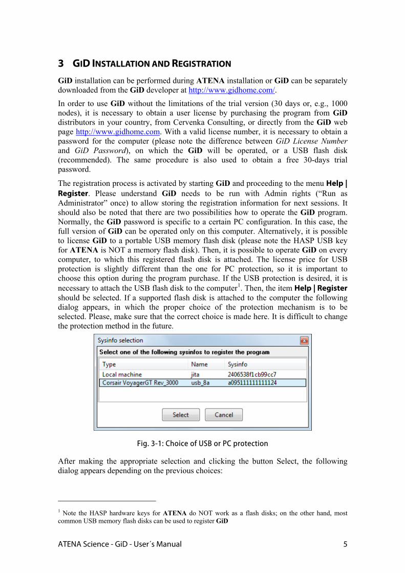
The registration process is activated by starting GiD and proceeding to the menu Help | Register. Please understand GiD needs to be run with Admin rights (“Run as Administrator” once) to allow storing the registration information for next sessions. It should also be noted that there are two possibilities how to operate the GiD program. Normally, the GiD password is specific to a certain PC configuration. In this case, the full version of GiD can be operated only on this computer. Alternatively, it is possible to license GiD to a portable USB memory flash disk (please note the HASP USB key for ATENA is NOT a memory flash disk). Then, it is possible to operate GiD on every computer, to which this registered flash disk is attached. The license price for USB protection is slightly different than the one for PC protection, so it is important to choose this option during the program purchase. If the USB protection is desired, it is necessary to attach the USB flash disk to the computer1. Then, the item Help | Register should be selected. If a supported flash disk is attached to the computer the following dialog appears, in which the proper choice of the protection mechanism is to be selected. Please, make sure that the correct choice is made here. It is difficult to change the protection method in the future.
Fig. 3-1: Choice of USB or PC protection
After making the appropriate selection and clicking the button Select, the following dialog appears depending on the previous choices:
1 Note the HASP hardware keys for ATENA do NOT work as a flash disks; on the other hand, most common USB memory flash disks can be used to register GiD
6
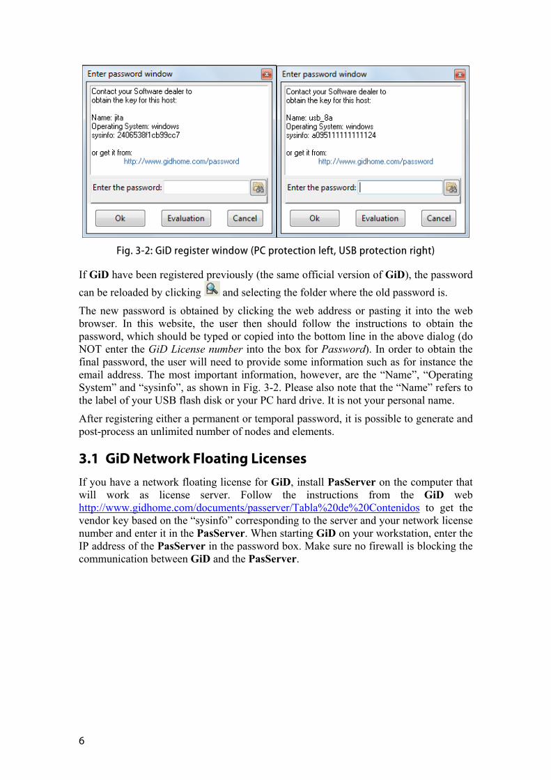
Fig. 3-2: GiD register window (PC protection left, USB protection right)
If GiD have been registered previously (the same official version of GiD), the password
can be reloaded by clicking and selecting the folder where the old password is.
The new password is obtained by clicking the web address or pasting it into the web browser. In this website, the user then should follow the instructions to obtain the password, which should be typed or copied into the bottom line in the above dialog (do NOT enter the GiD License number into the box for Password). In order to obtain the final password, the user will need to provide some information such as for instance the email address. The most important information, however, are the “Name”, “Operating System” and “sysinfo”, as shown in Fig. 3-2. Please also note that the “Name” refers to the label of your USB flash disk or your PC hard drive. It is not your personal name.
After registering either a permanent or temporal password, it is possible to generate and post-process an unlimited number of nodes and elements.
3.1 GiD Network Floating Licenses If you have a network floating license for GiD, install PasServer on the computer that will work as license server. Follow the instructions from the GiD web http://www.gidhome.com/documents/passerver/Tabla%20de%20Contenidos to get the vendor key based on the “sysinfo” corresponding to the server and your network license number and enter it in the PasServer. When starting GiD on your workstation, enter the IP address of the PasServer in the password box. Make sure no firewall is blocking the communication between GiD and the PasServer.
ATENA Science - GiD - User´s Manual 7
4 ATENA-GID INSTALLATION The installation of ATENA-GiD interface can be performed using the ATENA installer. Please make sure the ATENA-GiD interface is selected for installation. During this process, the user needs to confirm the location of the GiD directory.
New problem types related to ATENA should appear in the GiD menu. The problem types are available under the GiD menu Data | Problem type. If the ATENA problem types are not shown there, most likely, you have installed a new GiD version after ATENA has been installed, or have multiple GiD versions installed, and have installed the ATENA-GiD scripts into another one than you are using. To fix the issue, you can re-run the ATENA setup and select the ATENA-GiD interface to be installed for the GiD version you wish to work with (do not forget to expand the ATENA Science branch at the selection page of the installer).
4.1 Manual Installation of the ATENA-GiD Scripts Alternatively, the ATENA-GiD interface can be also installed manually as it is described in the following paragraphs.
1. Download the ATENA-GiD version corresponding to your ATENA version from the Downloads section of www.cervenka.cz and unpack the archive to your hard disk.
1.a You can also find the scripts in the installation directory of another GiD version, e.g., if you have just installed a new GiD version and were using ATENA with an older GiD version previously.
2. Copy the Atena directory tree into the Problem types directory of the GiD version you like to use with ATENA. On most computers, the GiD is installed in the directory:
C:\Program Files\GiD\GiDx.x
e.g., if you use GiD 10.0.9, copy the Atena tree into
C:\Program Files\GiD\GiD10.0.9\problemtypes\Atena
3. Start GiD and check if the new problem types appear in the GiD menu.
In order to be able to directly launch ATENA analysis and ATENA post-processing directly from GiD the following environmental variables are to be defined on your computer:
32bit
SET AtenaWin="%programfiles%\CervenkaConsulting\AtenaV5\AtenaWin.exe"
SET AtenaConsole="%programfiles%\CervenkaConsulting\AtenaV5\AtenaConsole.exe"
SET AtenaStudio="%programfiles%\CervenkaConsulting\AtenaV5\AtenaStudio.exe"
SET AtenaResults2GiD="%programfiles%\CervenkaConsulting\AtenaV5\A2G.exe"
64bit

8
SET AtenaWin64="%programfiles%\CervenkaConsulting\AtenaV5x64\AtenaWin64.exe"
SET AtenaConsole64="%programfiles%\CervenkaConsulting\AtenaV5x64\AtenaConsole64.exe"
SET AtenaStudio64="%programfiles%\CervenkaConsulting\AtenaV5x64\AtenaStudio.exe"
Where the path should point to the appropriate location, where the programs are installed.
ATENA Science - GiD - User´s Manual 9
5 ATENA - SPECIFIC COMMANDS
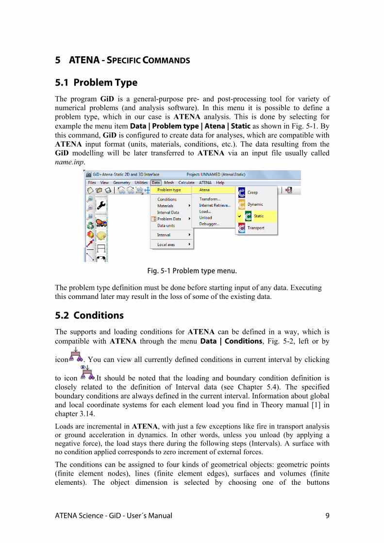
5.1 Problem Type The program GiD is a general-purpose pre- and post-processing tool for variety of numerical problems (and analysis software). In this menu it is possible to define a problem type, which in our case is ATENA analysis. This is done by selecting for example the menu item Data | Problem type | Atena | Static as shown in Fig. 5-1. By this command, GiD is configured to create data for analyses, which are compatible with ATENA input format (units, materials, conditions, etc.). The data resulting from the GiD modelling will be later transferred to ATENA via an input file usually called name.inp.
Fig. 5-1 Problem type menu.
The problem type definition must be done before starting input of any data. Executing this command later may result in the loss of some of the existing data.
5.2 Conditions The supports and loading conditions for ATENA can be defined in a way, which is compatible with ATENA through the menu Data | Conditions, Fig. 5-2, left or by
icon . You can view all currently defined conditions in current interval by clicking
to icon .It should be noted that the loading and boundary condition definition is closely related to the definition of Interval data (see Chapter 5.4). The specified boundary conditions are always defined in the current interval. Information about global and local coordinate systems for each element load you find in Theory manual [1] in chapter 3.14.
Loads are incremental in ATENA, with just a few exceptions like fire in transport analysis or ground acceleration in dynamics. In other words, unless you unload (by applying a negative force), the load stays there during the following steps (Intervals). A surface with no condition applied corresponds to zero increment of external forces.
The conditions can be assigned to four kinds of geometrical objects: geometric points (finite element nodes), lines (finite element edges), surfaces and volumes (finite elements). The object dimension is selected by choosing one of the buttons
10
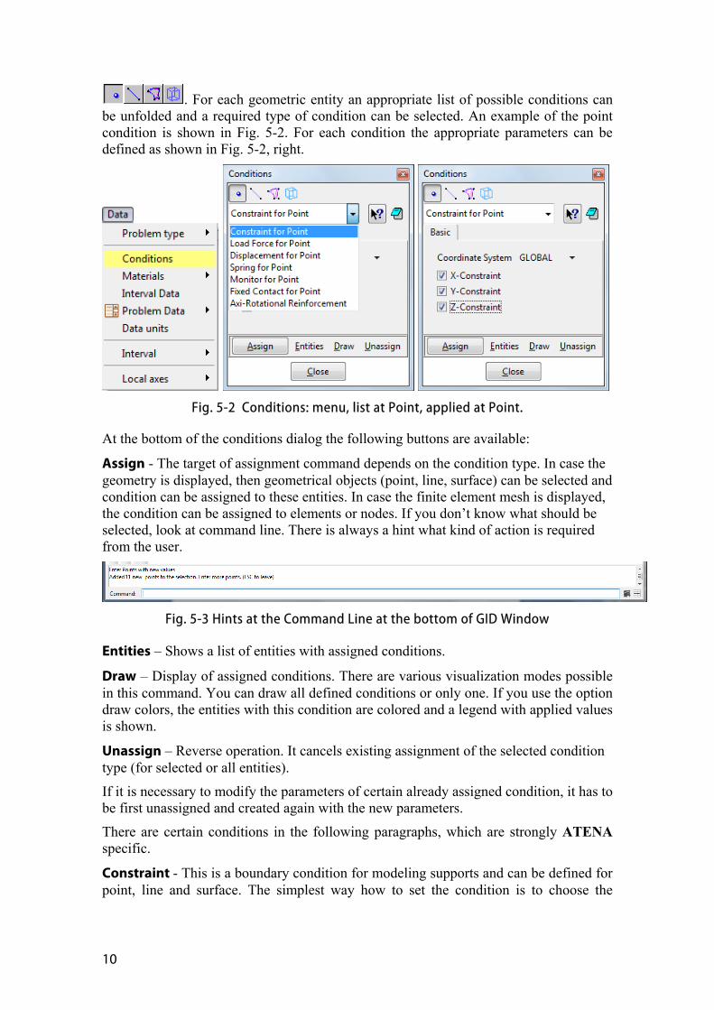
. For each geometric entity an appropriate list of possible conditions can be unfolded and a required type of condition can be selected. An example of the point condition is shown in Fig. 5-2. For each condition the appropriate parameters can be defined as shown in Fig. 5-2, right.
Fig. 5-2 Conditions: menu, list at Point, applied at Point.
At the bottom of the conditions dialog the following buttons are available:
Assign - The target of assignment command depends on the condition type. In case the geometry is displayed, then geometrical objects (point, line, surface) can be selected and condition can be assigned to these entities. In case the finite element mesh is displayed, the condition can be assigned to elements or nodes. If you don’t know what should be selected, look at command line. There is always a hint what kind of action is required from the user.
Fig. 5-3 Hints at the Command Line at the bottom of GID Window
Entities – Shows a list of entities with assigned conditions.
Draw – Display of assigned conditions. There are various visualization modes possible in this command. You can draw all defined conditions or only one. If you use the option draw colors, the entities with this condition are colored and a legend with applied values is shown.
Unassign – Reverse operation. It cancels existing assignment of the selected condition type (for selected or all entities).
If it is necessary to modify the parameters of certain already assigned condition, it has to be first unassigned and created again with the new parameters.
There are certain conditions in the following paragraphs, which are strongly ATENA specific.
Constraint - This is a boundary condition for modeling supports and can be defined for point, line and surface. The simplest way how to set the condition is to choose the
ATENA Science - GiD - User´s Manual 11
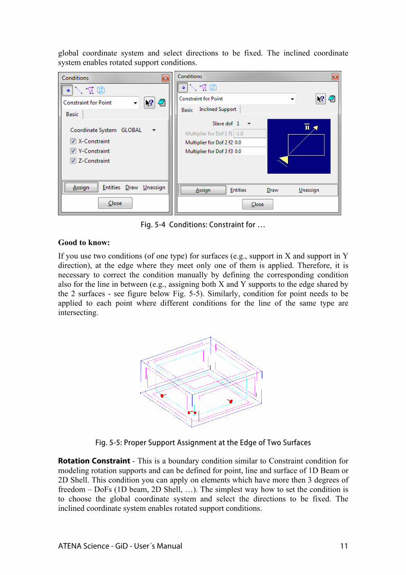
global coordinate system and select directions to be fixed. The inclined coordinate system enables rotated support conditions.
Fig. 5-4 Conditions: Constraint for …
Good to know:
If you use two conditions (of one type) for surfaces (e.g., support in X and support in Y direction), at the edge where they meet only one of them is applied. Therefore, it is necessary to correct the condition manually by defining the corresponding condition also for the line in between (e.g., assigning both X and Y supports to the edge shared by the 2 surfaces - see figure below Fig. 5-5). Similarly, condition for point needs to be applied to each point where different conditions for the line of the same type are intersecting.
Fig. 5-5: Proper Support Assignment at the Edge of Two Surfaces
Rotation Constraint - This is a boundary condition similar to Constraint condition for modeling rotation supports and can be defined for point, line and surface of 1D Beam or 2D Shell. This condition you can apply on elements which have more then 3 degrees of freedom – DoFs (1D beam, 2D Shell, …). The simplest way how to set the condition is to choose the global coordinate system and select the directions to be fixed. The inclined coordinate system enables rotated support conditions.
12
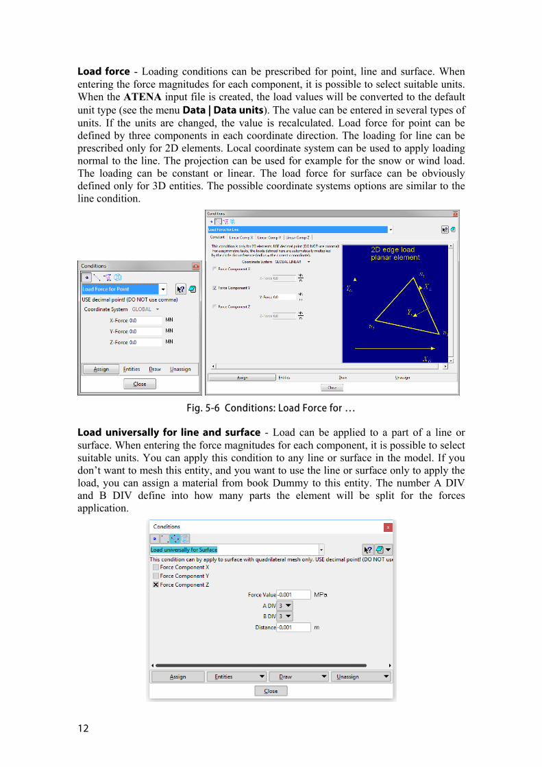
Load force - Loading conditions can be prescribed for point, line and surface. When entering the force magnitudes for each component, it is possible to select suitable units. When the ATENA input file is created, the load values will be converted to the default unit type (see the menu Data | Data units). The value can be entered in several types of units. If the units are changed, the value is recalculated. Load force for point can be defined by three components in each coordinate direction. The loading for line can be prescribed only for 2D elements. Local coordinate system can be used to apply loading normal to the line. The projection can be used for example for the snow or wind load. The loading can be constant or linear. The load force for surface can be obviously defined only for 3D entities. The possible coordinate systems options are similar to the line condition.
Fig. 5-6 Conditions: Load Force for …
Load universally for line and surface - Load can be applied to a part of a line or surface. When entering the force magnitudes for each component, it is possible to select suitable units. You can apply this condition to any line or surface in the model. If you don’t want to mesh this entity, and you want to use the line or surface only to apply the load, you can assign a material from book Dummy to this entity. The number A DIV and B DIV define into how many parts the element will be split for the forces application.
ATENA Science - GiD - User´s Manual 13
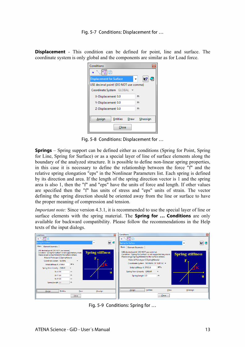
Fig. 5-7 Conditions: Displacement for …
Displacement - This condition can be defined for point, line and surface. The coordinate system is only global and the components are similar as for Load force.
Fig. 5-8 Conditions: Displacement for …
Springs – Spring support can be defined either as conditions (Spring for Point, Spring for Line, Spring for Surface) or as a special layer of line of surface elements along the boundary of the analyzed structure. It is possible to define non-linear spring properties, in this case it is necessary to define the relationship between the force "f" and the relative spring elongation "eps" in the Nonlinear Parameters list. Each spring is defined by its direction and area. If the length of the spring direction vector is 1 and the spring area is also 1, then the "f" and "eps" have the units of force and length. If other values are specified then the "f" has units of stress and "eps" units of strain. The vector defining the spring direction should be oriented away from the line or surface to have the proper meaning of compression and tension.
Important note: Since version 4.3.1, it is recommended to use the special layer of line or surface elements with the spring material. The Spring for … Conditions are only available for backward compatibility. Please follow the recommendations in the Help texts of the input dialogs.
Fig. 5-9 Conditions: Spring for …
14
For instance in order to define a surface spring with 5kN/m2 pressure at 15mm displacement:
1. set the spring length to 1m, then 15mm displacement corresponds to relative displacement (elongation/shortening) 0.015 m.
2. set the spring material stiffness to 0.005 [MN] / 0.015 = 0.3333333 MPa ( E )
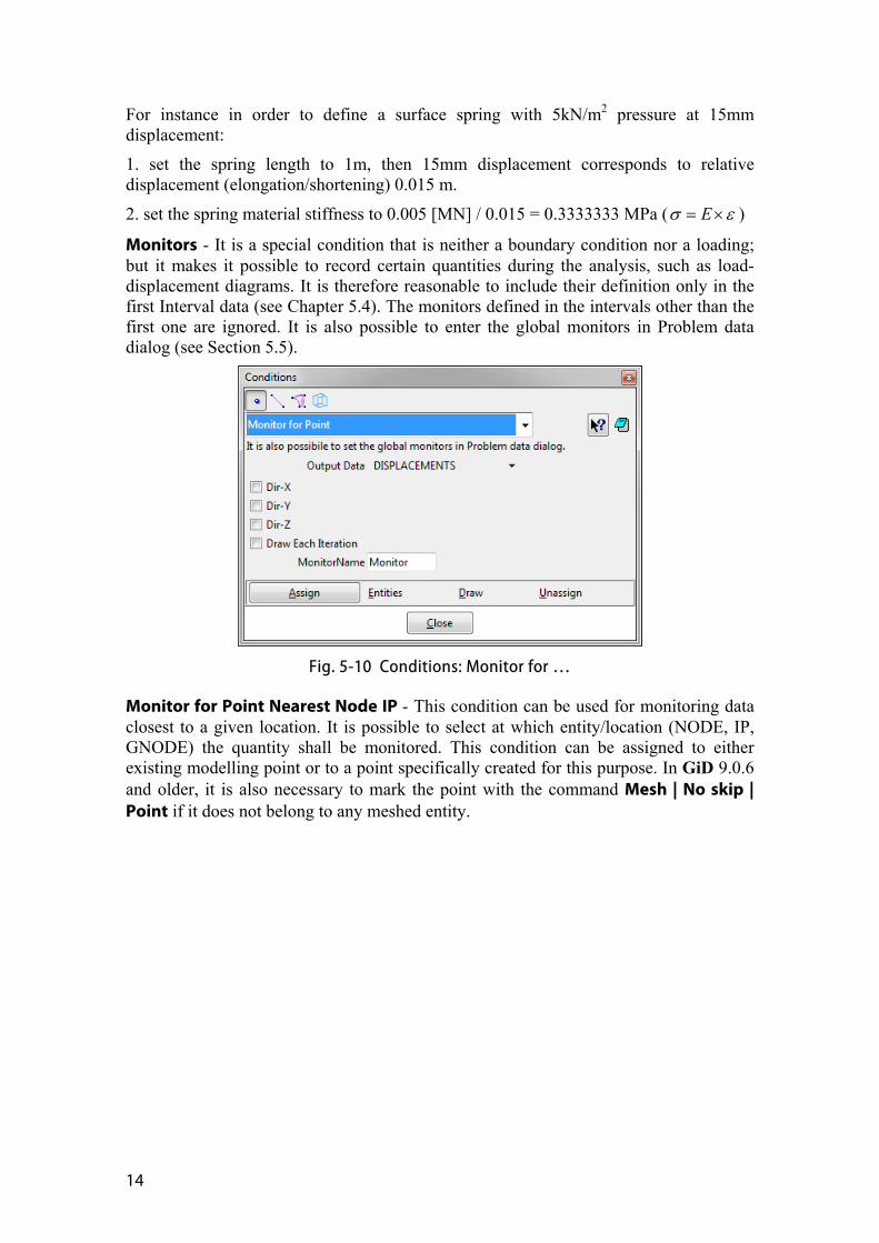
Monitors - It is a special condition that is neither a boundary condition nor a loading; but it makes it possible to record certain quantities during the analysis, such as load-displacement diagrams. It is therefore reasonable to include their definition only in the first Interval data (see Chapter 5.4). The monitors defined in the intervals other than the first one are ignored. It is also possible to enter the global monitors in Problem data dialog (see Section 5.5).
Fig. 5-10 Conditions: Monitor for …
Monitor for Point Nearest Node IP - This condition can be used for monitoring data closest to a given location. It is possible to select at which entity/location (NODE, IP, GNODE) the quantity shall be monitored. This condition can be assigned to either existing modelling point or to a point specifically created for this purpose. In GiD 9.0.6 and older, it is also necessary to mark the point with the command Mesh | No skip | Point if it does not belong to any meshed entity.
ATENA Science - GiD - User´s Manual 15
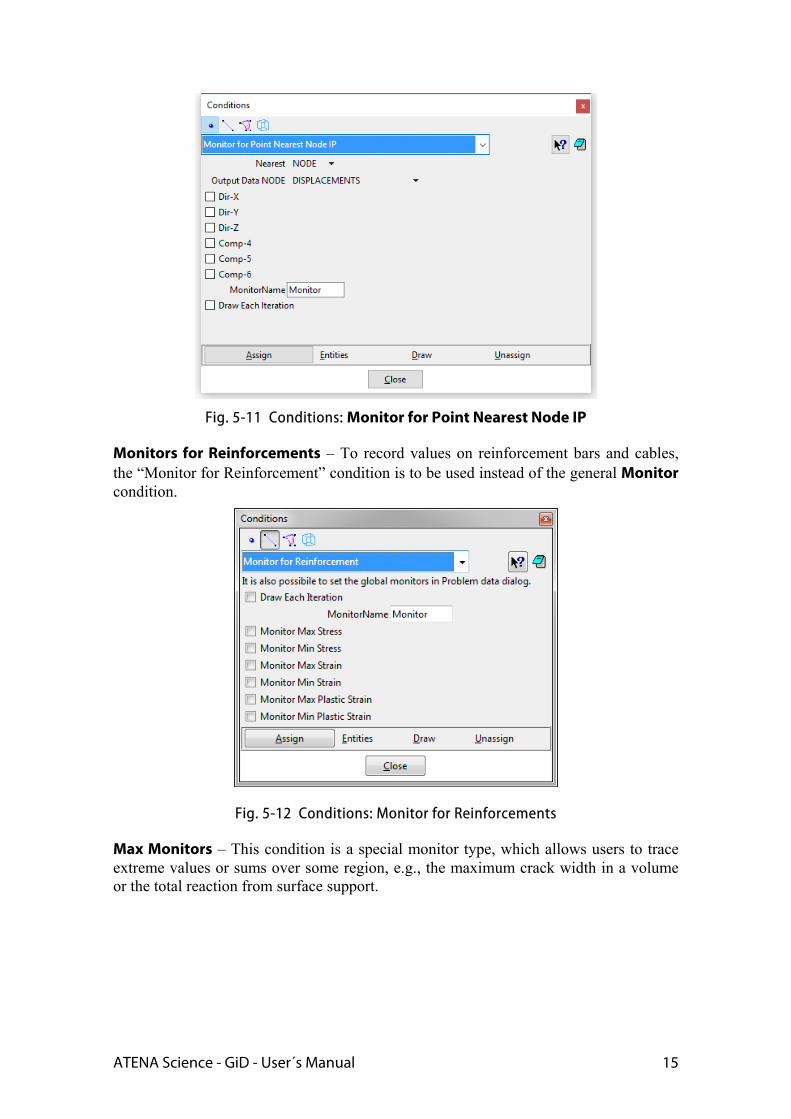
Fig. 5-11 Conditions: Monitor for Point Nearest Node IP
Monitors for Reinforcements – To record values on reinforcement bars and cables, the “Monitor for Reinforcement” condition is to be used instead of the general Monitor condition.
Fig. 5-12 Conditions: Monitor for Reinforcements
Max Monitors – This condition is a special monitor type, which allows users to trace extreme values or sums over some region, e.g., the maximum crack width in a volume or the total reaction from surface support.
16
Fig. 5-13 Conditions: Max Monitor for …
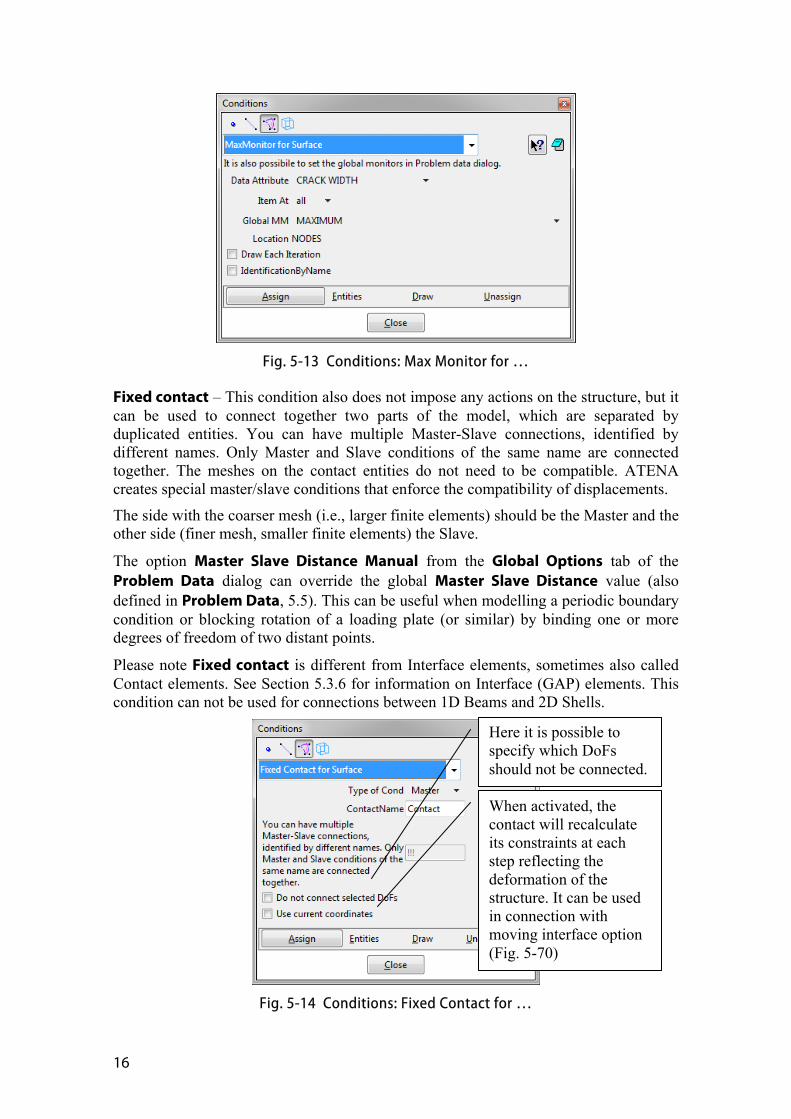
Fixed contact – This condition also does not impose any actions on the structure, but it can be used to connect together two parts of the model, which are separated by duplicated entities. You can have multiple Master-Slave connections, identified by different names. Only Master and Slave conditions of the same name are connected together. The meshes on the contact entities do not need to be compatible. ATENA creates special master/slave conditions that enforce the compatibility of displacements.
The side with the coarser mesh (i.e., larger finite elements) should be the Master and the other side (finer mesh, smaller finite elements) the Slave.
The option Master Slave Distance Manual from the Global Options tab of the Problem Data dialog can override the global Master Slave Distance value (also defined in Problem Data, 5.5). This can be useful when modelling a periodic boundary condition or blocking rotation of a loading plate (or similar) by binding one or more degrees of freedom of two distant points.
Please note Fixed contact is different from Interface elements, sometimes also called Contact elements. See Section 5.3.6 for information on Interface (GAP) elements. This condition can not be used for connections between 1D Beams and 2D Shells.
Fig. 5-14 Conditions: Fixed Contact for …
Here it is possible to specify which DoFs should not be connected.
When activated, the contact will recalculate its constraints at each step reflecting the deformation of the structure. It can be used in connection with moving interface option (Fig. 5-70)
ATENA Science - GiD - User´s Manual 17
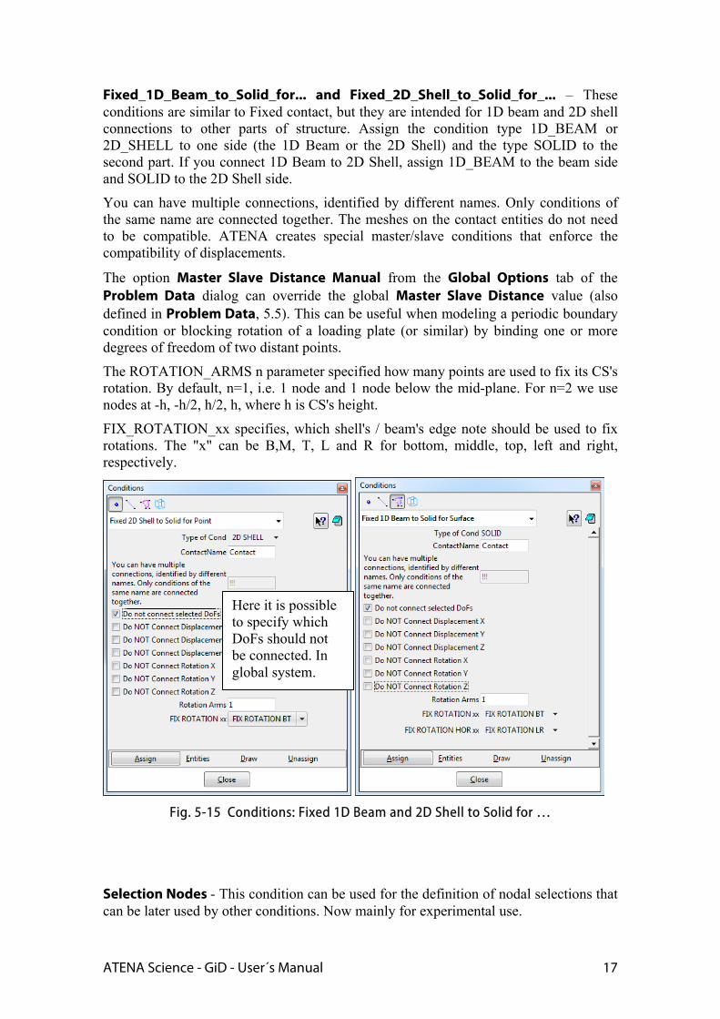
Fixed_1D_Beam_to_Solid_for... and Fixed_2D_Shell_to_Solid_for_... – These conditions are similar to Fixed contact, but they are intended for 1D beam and 2D shell connections to other parts of structure. Assign the condition type 1D_BEAM or 2D_SHELL to one side (the 1D Beam or the 2D Shell) and the type SOLID to the second part. If you connect 1D Beam to 2D Shell, assign 1D_BEAM to the beam side and SOLID to the 2D Shell side.
You can have multiple connections, identified by different names. Only conditions of the same name are connected together. The meshes on the contact entities do not need to be compatible. ATENA creates special master/slave conditions that enforce the compatibility of displacements.
The option Master Slave Distance Manual from the Global Options tab of the Problem Data dialog can override the global Master Slave Distance value (also defined in Problem Data, 5.5). This can be useful when modeling a periodic boundary condition or blocking rotation of a loading plate (or similar) by binding one or more degrees of freedom of two distant points.
The ROTATION_ARMS n parameter specified how many points are used to fix its CS's rotation. By default, n=1, i.e. 1 node and 1 node below the mid-plane. For n=2 we use nodes at -h, -h/2, h/2, h, where h is CS's height.
FIX_ROTATION_xx specifies, which shell's / beam's edge note should be used to fix rotations. The "x" can be B,M, T, L and R for bottom, middle, top, left and right, respectively.
Fig. 5-15 Conditions: Fixed 1D Beam and 2D Shell to Solid for …
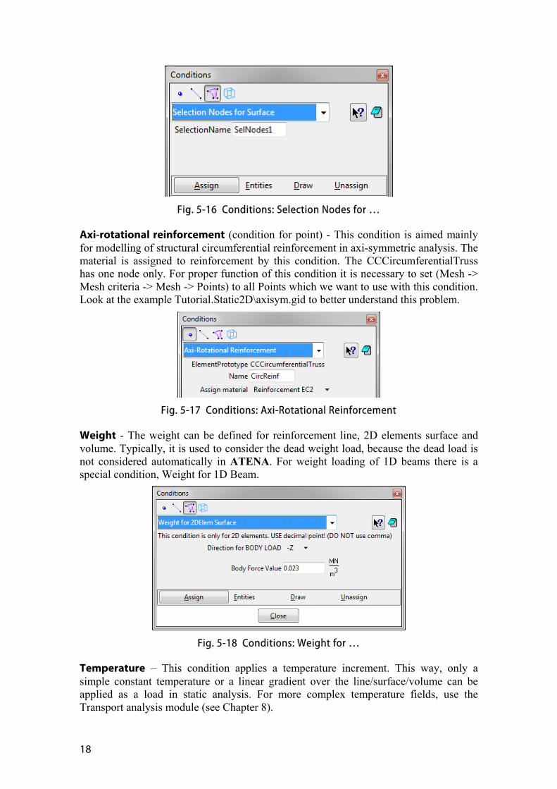
Selection Nodes - This condition can be used for the definition of nodal selections that can be later used by other conditions. Now mainly for experimental use.
Here it is possible to specify which DoFs should not be connected. In global system.
18
Fig. 5-16 Conditions: Selection Nodes for …
Axi-rotational reinforcement (condition for point) - This condition is aimed mainly for modelling of structural circumferential reinforcement in axi-symmetric analysis. The material is assigned to reinforcement by this condition. The CCCircumferentialTruss has one node only. For proper function of this condition it is necessary to set (Mesh -> Mesh criteria -> Mesh -> Points) to all Points which we want to use with this condition. Look at the example Tutorial.Static2D\axisym.gid to better understand this problem.
Fig. 5-17 Conditions: Axi-Rotational Reinforcement
Weight - The weight can be defined for reinforcement line, 2D elements surface and volume. Typically, it is used to consider the dead weight load, because the dead load is not considered automatically in ATENA. For weight loading of 1D beams there is a special condition, Weight for 1D Beam.
Fig. 5-18 Conditions: Weight for …
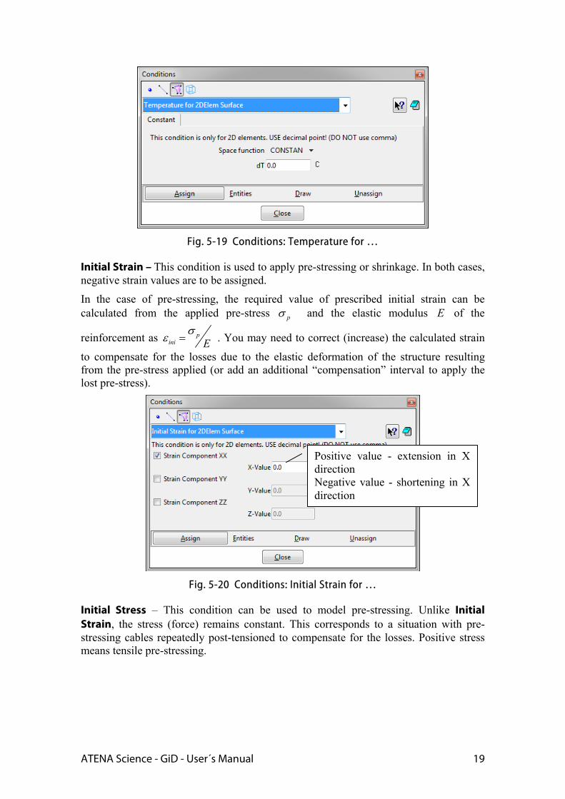
Temperature – This condition applies a temperature increment. This way, only a simple constant temperature or a linear gradient over the line/surface/volume can be applied as a load in static analysis. For more complex temperature fields, use the Transport analysis module (see Chapter 8).
ATENA Science - GiD - User´s Manual 19
Fig. 5-19 Conditions: Temperature for …
Initial Strain – This condition is used to apply pre-stressing or shrinkage. In both cases, negative strain values are to be assigned.
In the case of pre-stressing, the required value of prescribed initial strain can be calculated from the applied pre-stress p and the elastic modulus E of the
reinforcement as pini E
. You may need to correct (increase) the calculated strain
to compensate for the losses due to the elastic deformation of the structure resulting from the pre-stress applied (or add an additional “compensation” interval to apply the lost pre-stress).
Fig. 5-20 Conditions: Initial Strain for …
Initial Stress – This condition can be used to model pre-stressing. Unlike Initial Strain, the stress (force) remains constant. This corresponds to a situation with pre-stressing cables repeatedly post-tensioned to compensate for the losses. Positive stress means tensile pre-stressing.
Positive value - extension in X direction Negative value - shortening in X direction
20
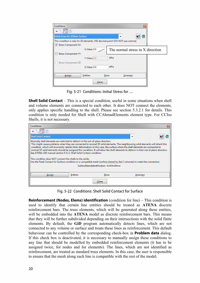
Fig. 5-21 Conditions: Initial Stress for …
Shell Solid Contact – This is a special condition, useful in some situations when shell and volume elements are connected to each other. It does NOT connect the elements, only applies specific handling to the shell. Please see section 5.3.2.1 for details. This condition is only needed for Shell with CCAhmadElements element type. For CCIso Shells, it is not necessary.
Fig. 5-22 Conditions: Shell Solid Contact for Surface
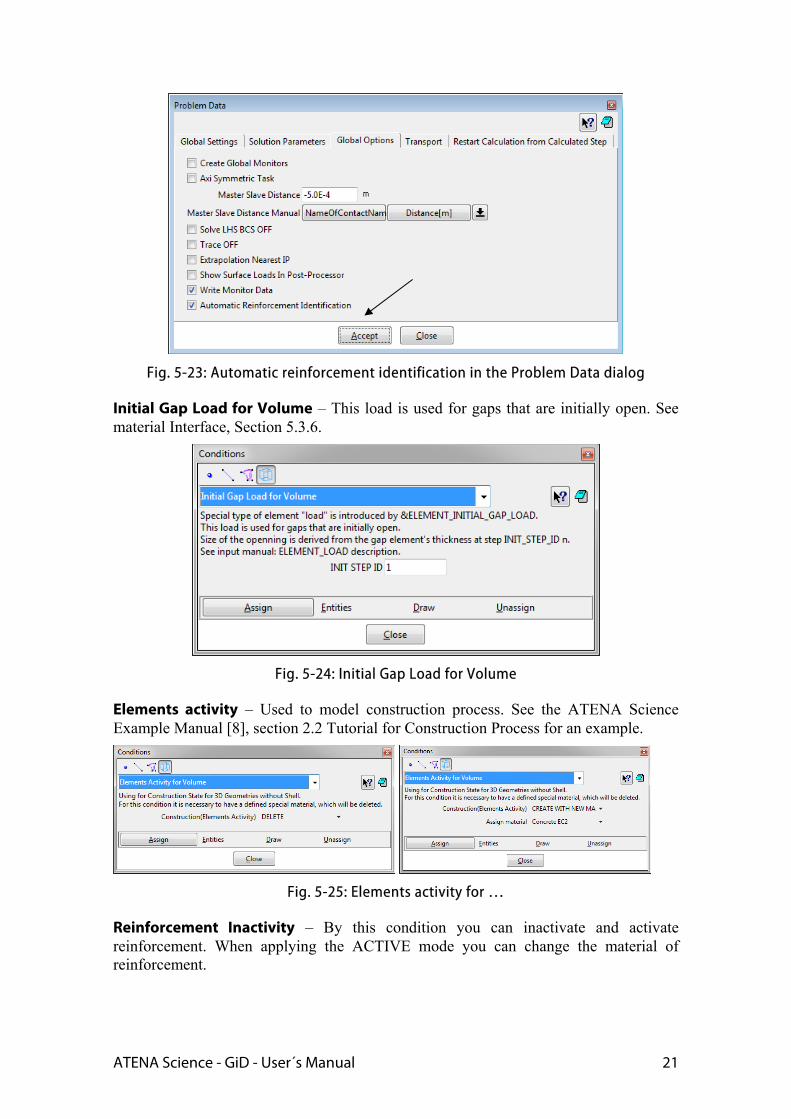
Reinforcement (Nodes, Elems) identification (condition for line) – This condition is used to identify that certain line entities should be treated as ATENA discrete reinforcement bars. The truss elements, which will be generated along these entities, will be embedded into the ATENA model as discrete reinforcement bars. This means that they will be further subdivided depending on their intersections with the solid finite elements. By default, the GiD program automatically detects lines, which are not connected to any volume or surface and treats these lines as reinforcement. This default behaviour can be controlled by the corresponding check-box in Problem data dialog. If this check box is deactivated, it is necessary to manually assign these conditions to any line that should be modelled by embedded reinforcement elements (it has to be assigned twice, for nodes and for elements). The lines, which are not identified as reinforcement, are treated as standard truss elements. In this case, the user is responsible to ensure that the mesh along each line is compatible with the rest of the model.
The normal stress in X direction
ATENA Science - GiD - User´s Manual 21
Fig. 5-23: Automatic reinforcement identification in the Problem Data dialog
Initial Gap Load for Volume – This load is used for gaps that are initially open. See material Interface, Section 5.3.6.
Fig. 5-24: Initial Gap Load for Volume
Elements activity – Used to model construction process. See the ATENA Science Example Manual [8], section 2.2 Tutorial for Construction Process for an example.
Fig. 5-25: Elements activity for …
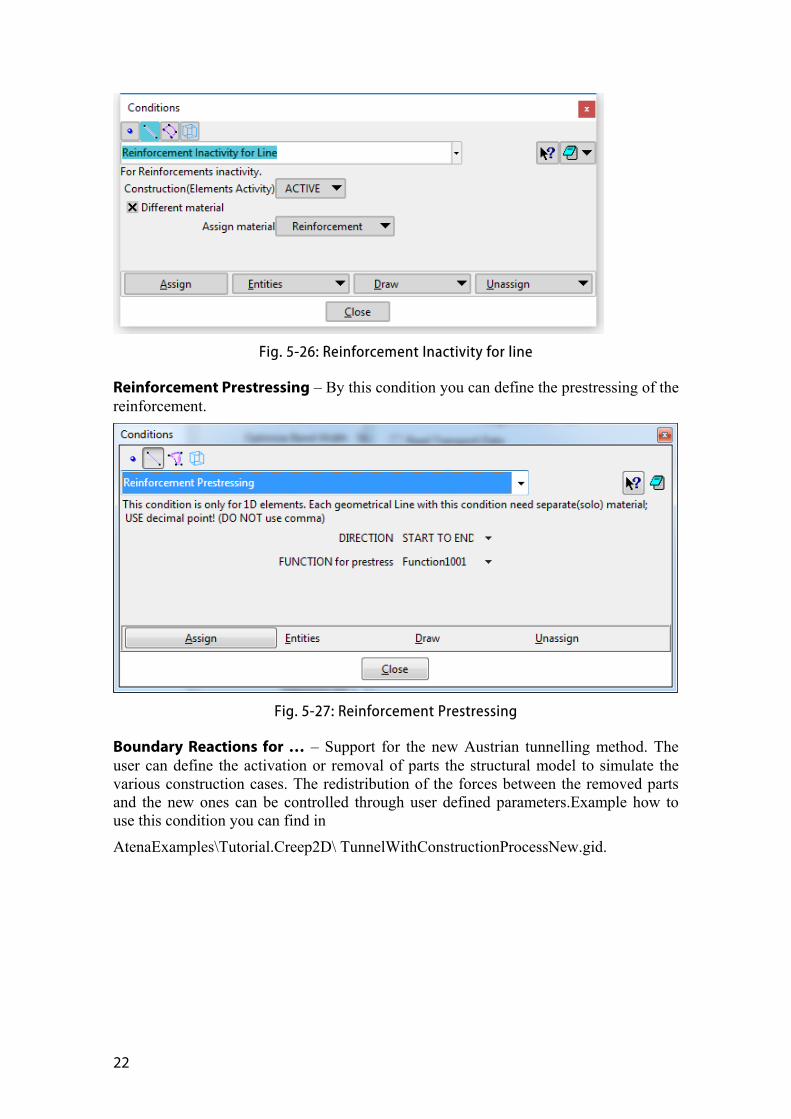
Reinforcement Inactivity – By this condition you can inactivate and activate reinforcement. When applying the ACTIVE mode you can change the material of reinforcement.
22
Fig. 5-26: Reinforcement Inactivity for line
Reinforcement Prestressing – By this condition you can define the prestressing of the reinforcement.
Fig. 5-27: Reinforcement Prestressing
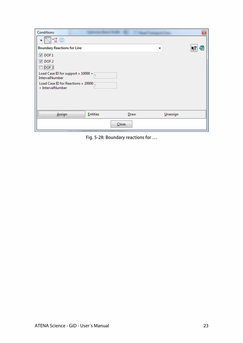
Boundary Reactions for … – Support for the new Austrian tunnelling method. The user can define the activation or removal of parts the structural model to simulate the various construction cases. The redistribution of the forces between the removed parts and the new ones can be controlled through user defined parameters.Example how to use this condition you can find in
AtenaExamples\Tutorial.Creep2D\ TunnelWithConstructionProcessNew.gid.
ATENA Science - GiD - User´s Manual 23
Fig. 5-28: Boundary reactions for …
24
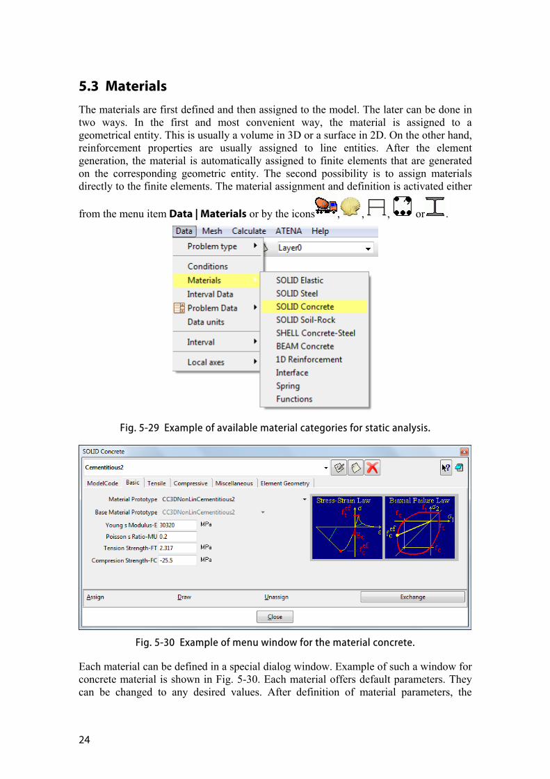
5.3 Materials The materials are first defined and then assigned to the model. The later can be done in two ways. In the first and most convenient way, the material is assigned to a geometrical entity. This is usually a volume in 3D or a surface in 2D. On the other hand, reinforcement properties are usually assigned to line entities. After the element generation, the material is automatically assigned to finite elements that are generated on the corresponding geometric entity. The second possibility is to assign materials directly to the finite elements. The material assignment and definition is activated either
from the menu item Data | Materials or by the icons , , , or .
Fig. 5-29 Example of available material categories for static analysis.
Fig. 5-30 Example of menu window for the material concrete.
Each material can be defined in a special dialog window. Example of such a window for concrete material is shown in Fig. 5-30. Each material offers default parameters. They can be changed to any desired values. After definition of material parameters, the
ATENA Science - GiD - User´s Manual 25
material can be assigned to the numerical model. Operations for material assignment are done with the buttons in the bottom of the dialog.
Assign - The target of assignment command depends on the display type. In case that geometry is displayed, then geometry type is to be selected (line for reinforcement, volume for concrete), and material can be assigned to the geometric entities. In case that the finite elements are displayed, the material can be directly assigned to individual finite elements. It should be noted that if a material is assigned directly to finite elements, the assignment is lost every time the mesh is regenerated.
Draw – displays the material assignment to volumes or elements.
Unassisgn – Reverse operation to Assign. It deletes the material assignment.
Exchange – Open material database from other GiD project and import your created material to your new project. It is also possible to import material from new project to the other project (exchange).
Table 1: Materials supported by GiD interface to ATENA
GiD name ATENA name (INP command) Description
SOLID Elastic
Elastic 3D CC3DElastIsotropic Linear elastic isotropic materials for 3D
SOLID Steel
Steel Von Mises 3D CC3DBiLinearSteelVonMises Plastic materials with Von-Mises yield condition, e.g. suitable for steel.
Steel Von Mises 3D CC3DBiLinearVonMisesWithTempDepPropertiess
This model is to be used to simulate change of material properties due to current temperature. The temperature fields can be imported from a previously performed thermal analysis.
SOLID Concrete
Concrete EC2 CC3DNonLinCementitious2 Material is like Cementitious2. You can generate material properties according the EC2
Cementitious2
CC3DNonLinCementitious2 Materials suitable for rock or concrete like materials. This material is identical to 3DNONLINCEMENTITIOUS except that this model is fully incremental.
Cementitious2 CC3DNonLinCementitious2Fatigue
This material is based on the CC3DNonLinCementitious2 material, extended for fatigue calculation.
Cementitious2 CC3DNonLinCementitious2WithTempDepProperties
This model is to be used to simulate change of material properties due to current temperature. The temperature fields can be imported from a previously performed thermal analysis.
26
Cementitious2 User CC3DNonLinCementitious2User Materials suitable for rock or concrete like materials. This material is identical to CC3DNonLinCementitious2 except that selected material laws can be defined by user curves (5.3.1.4).
Cementitious2 SHCC CC3DNonLinCementitious2SHCC Strain Hardening Cementitious Composite material. Material suitable for fiber reinforced concrete, such as SHCC and HPFRCC materials. Identical to CC3DNonLinCementitious2User except for the shear response definition.
Cementitious3 CC3DNonLinCementitious3 Materials suitable for rock or concrete like materials. This material is an advanced version of CC3DNonLinCementitious2 material that can handle the increased deformation capacity of concrete under triaxial compression. Suitable for problems including confinement effects.
Reinforced Concrete CCCombinedMaterial This material can be used to create a composite material consisting of various components, such as for instance concrete with smeared reinforcement in various directions. Unlimited number of components can be specified. Output data for each component are then indicated by the label #i. Where i indicates a value of the i-th component. Described in section 5.3.4.
Microplane M4, M7 CCMicroplane4, CCMicroplane7 Bazant Microplane material models for concrete
SBETA Material CCSBETAMaterial Older version of the basic material for concrete, only suitable for 2-D plane stress models
only for Transport PROBLEM TYPE
Bazant_Xi_1994 CCModelBaXi94 Material for transport analysis (Transport3D PROBLEMTYPE ) – only supported for backward compatibility since ATENA 5.0 (CCTransportMaterial is now recommended), see section 8.1.2 for details.
CCTransportMaterial CCTransportMaterial Material for transport analysis, see section 8.1.1.
SOLID_Creep_Concrete (only for Creep PROBLEM TYPE)
ModelB3 CCModelB3 Bazant-Baweja B3 model
ModelB3Improved CCModelB3Improved model same as the above with support for specified time and humidity history
ModelBP_KX CCModelBP_KX creep model developed by Bazant-Kim, 1991.
ModelCEB_FIP78 CCModelCEB_FIP78 creep model advocated by CEB-FIP 1978
ModelCSN731201 CCModelCSN731201 model recommended by CSN731202
ModelBP1 CCModelBP1 full version of the creep model developed by Bazant-Panulla
ModelBP2 CCModelBP2 simplified version of the above model
ModelACI78 CCModelACI78 creep model by ACI Committee in 1978.
ATENA Science - GiD - User´s Manual 27
SOLID Soil-Rock
Drucker Prager CC3DDruckerPragerPlasticity Plastic materials with Drucker-Prager yield condition.
SHELL Concrete-Steel
Shell Concrete-Steel CCShellMaterial Shell geometry with support Ahmad elements, described in section 5.3.2.
These elements are reduced from a quadratic 3D brick element with 20 nodes. The element has 9 integration points in shell plane and layers in direction normal to its plane. The total number of integration points is 9x(number of layers). Important feature of shell element is, that its local Z axis must be perpendicular to the top surface of shell plane. The top surface is the surface on which the positive Z-axis points out of the shell. Other two axes, X and Y, must be in the shell plane. Such orientation must be ensured by user.
In each shell node there are 3 displacement degrees of freedom and corresponding nodal forces. However, some DOFs are not free due to introduction of kinematic constrains ensuring shell displacement model. For more details see Theory Manual.
Shell material can be used only on 3D quadratic brick elements (5.7.2).
BEAM Concrete
Beam Concrete CCBeam3DMaterial Special material, which activates the usage of special fiber beam element suitable for large scale analysis of complex structures with large elements (see 5.3.3). The element is based on a similar beam element from BATHE(1982). It is fully nonlinear, in terms of its geometry and material response. It uses quadratic approximation of its shape, so it can be curvilinear, twisted, with variable dimensions of the cross-sections. Moreover, beam’s cross-sections can be of any shape, optionally even with holes. The element belongs to the group of isoparametric elements with Gauss integration along its axisand trapezoidal (Newton-Cotes) quadrature within the cross-section. The integration (or material) points are placed in a way similar to the layered concept applied to shell elements,however, the “layers” are located in both “s,t” directions.
Beam material can be used only on 3D quadratic brick elements (5.7.2).
28
1D Reinforcement
Reinforcement EC2 CCReinforcement Material is like “Reinforcement”. You can generate material properties according the EC2
Reinforcement CCReinforcement Material for discrete reinforcement – bars and cables (5.3.5)
Reinforcement CCReinforcementWithTempDepProperties
This model is to be used to simulate change of material properties due to current temperature. The temperature fields can be imported from a previously performed thermal analysis.
Reinforcement CC1DElastIsotropic One dimension elastic material (only supported for backward compatibility since ATENA 4.3.0)
Reinforcement CCCyclingReinforcement Material for cyclic reinforcement
Interface
Interface CC2DInterface, CC3DInterface Interface (GAP) material for 2D and 3D analysis. Please see section 5.3.6 for description and important advice how to create contact elements.
Spring
Spring Material CCSpringMaterial Material for spring type boundary condition elements, i.e. for truss element modeling a spring.
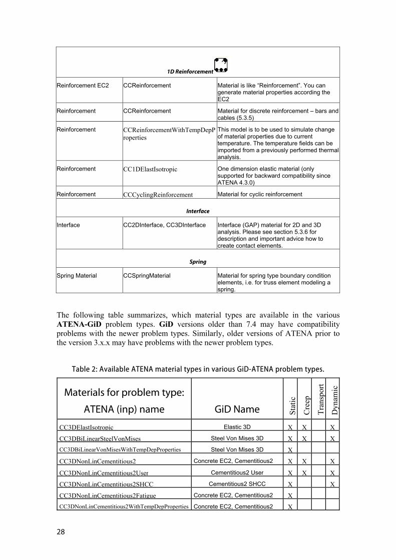
The following table summarizes, which material types are available in the various ATENA-GiD problem types. GiD versions older than 7.4 may have compatibility problems with the newer problem types. Similarly, older versions of ATENA prior to the version 3.x.x may have problems with the newer problem types.
Table 2: Available ATENA material types in various GiD-ATENA problem types.
Materials for problem type:
ATENA (inp) name
GiD Name Sta
tic
Cre
ep
Tra
nspo
rt
Dyn
amic
CC3DElastIsotropic Elastic 3D X X X
CC3DBiLinearSteelVonMises Steel Von Mises 3D X X X
CC3DBiLinearVonMisesWithTempDepProperties Steel Von Mises 3D X
CC3DNonLinCementitious2 Concrete EC2, Cementitious2 X X X
CC3DNonLinCementitious2User Cementitious2 User X X X
CC3DNonLinCementitious2SHCC Cementitious2 SHCC X X
CC3DNonLinCementitious2Fatigue Concrete EC2, Cementitious2 X
CC3DNonLinCementitious2WithTempDepProperties Concrete EC2, Cementitious2 X
ATENA Science - GiD - User´s Manual 29
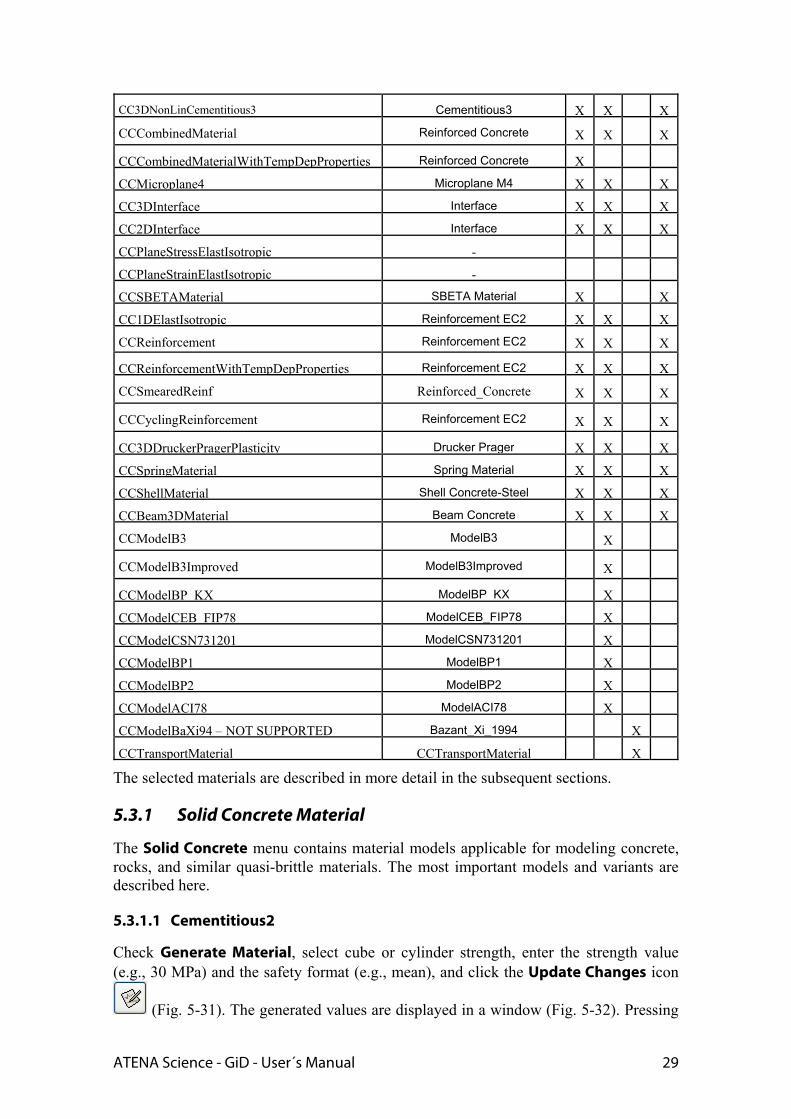
CC3DNonLinCementitious3 Cementitious3 X X X
CCCombinedMaterial Reinforced Concrete X X X
CCCombinedMaterialWithTempDepProperties Reinforced Concrete X
CCMicroplane4 Microplane M4 X X X
CC3DInterface Interface X X X
CC2DInterface Interface X X X
CCPlaneStressElastIsotropic -
CCPlaneStrainElastIsotropic -
CCSBETAMaterial SBETA Material X X
CC1DElastIsotropic Reinforcement EC2 X X X
CCReinforcement Reinforcement EC2 X X X
CCReinforcementWithTempDepProperties Reinforcement EC2 X X X
CCSmearedReinf Reinforced_Concrete X X X
CCCyclingReinforcement Reinforcement EC2 X X X
CC3DDruckerPragerPlasticity Drucker Prager X X X
CCSpringMaterial Spring Material X X X
CCShellMaterial Shell Concrete-Steel X X X
CCBeam3DMaterial Beam Concrete X X X
CCModelB3 ModelB3 X
CCModelB3Improved ModelB3Improved X
CCModelBP KX ModelBP_KX X
CCModelCEB FIP78 ModelCEB_FIP78 X
CCModelCSN731201 ModelCSN731201 X
CCModelBP1 ModelBP1 X
CCModelBP2 ModelBP2 X
CCModelACI78 ModelACI78 X
CCModelBaXi94 – NOT SUPPORTED Bazant_Xi_1994 X
CCTransportMaterial CCTransportMaterial X
The selected materials are described in more detail in the subsequent sections.
5.3.1 Solid Concrete Material
The Solid Concrete menu contains material models applicable for modeling concrete, rocks, and similar quasi-brittle materials. The most important models and variants are described here.
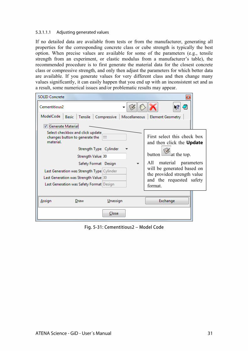
5.3.1.1 Cementitious2
Check Generate Material, select cube or cylinder strength, enter the strength value (e.g., 30 MPa) and the safety format (e.g., mean), and click the Update Changes icon
(Fig. 5-31). The generated values are displayed in a window (Fig. 5-32). Pressing
30
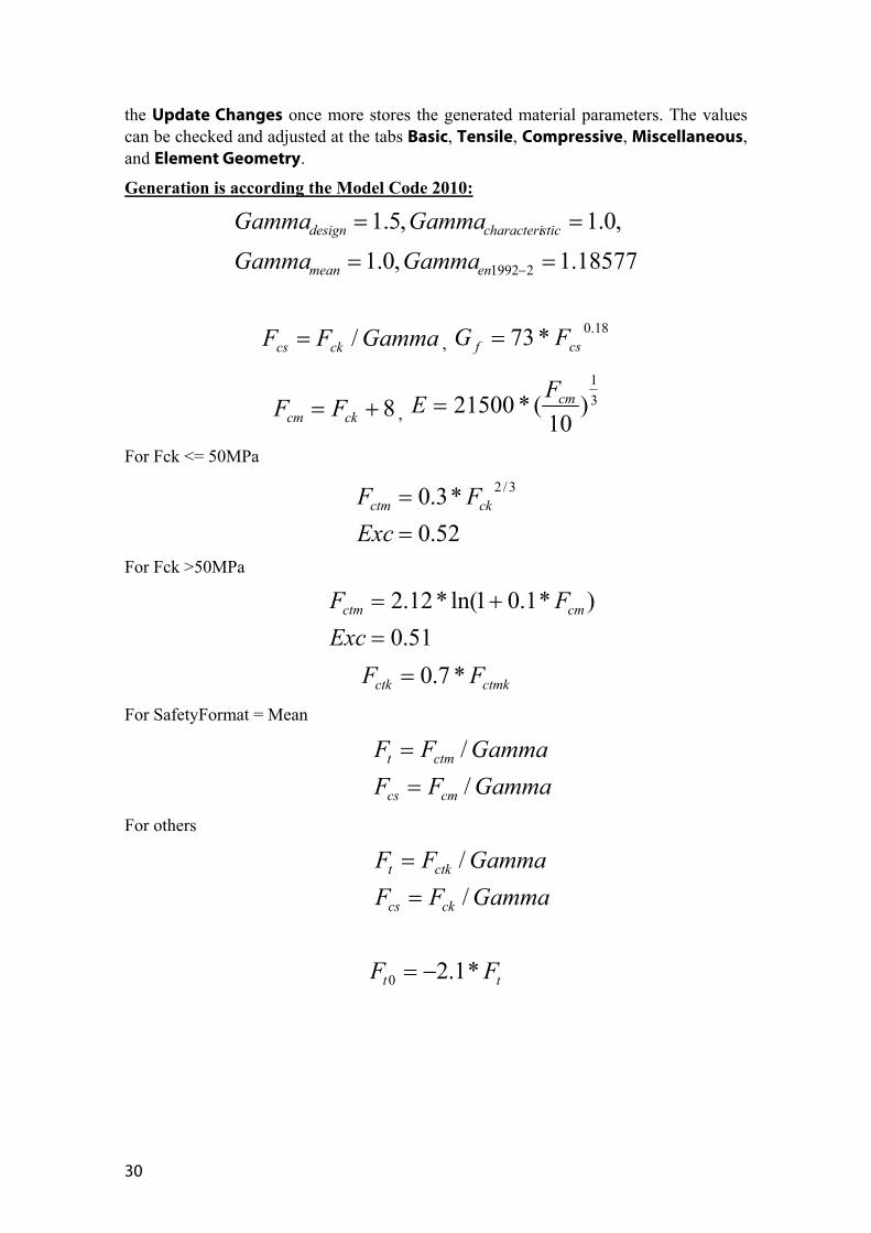
the Update Changes once more stores the generated material parameters. The values can be checked and adjusted at the tabs Basic, Tensile, Compressive, Miscellaneous, and Element Geometry.
Generation is according the Model Code 2010:
18577.1,0.1
,0.1,5.1
21992
enmean
sticcharacteridesign
GammaGamma
GammaGamma
GammaFF ckcs / , 18.0*73 csf FG
8 ckcm FF , 3
1
)10
(*21500 cmFE
For Fck <= 50MPa
52.0
*3.0 3/2
Exc
FF ckctm
For Fck >50MPa
51.0
)*1.01ln(*12.2
Exc
FF cmctm
ctmkctk FF *7.0
For SafetyFormat = Mean
GammaFF
GammaFF
cmcs
ctmt
/
/
For others
GammaFF
GammaFF
ckcs
ctkt
/
/
tt FF *1.20
ATENA Science - GiD - User´s Manual 31
5.3.1.1.1 Adjusting generated values
If no detailed data are available from tests or from the manufacturer, generating all properties for the corresponding concrete class or cube strength is typically the best option. When precise values are available for some of the parameters (e.g., tensile strength from an experiment, or elastic modulus from a manufacturer’s table), the recommended procedure is to first generate the material data for the closest concrete class or compressive strength, and only then adjust the parameters for which better data are available. If you generate values for very different class and then change many values significantly, it can easily happen that you end up with an inconsistent set and as a result, some numerical issues and/or problematic results may appear.
Fig. 5-31: Cementitious2 – Model Code
First select this check box and then click the Update
button at the top.
All material parameters will be generated based on the provided strength value and the requested safety format.
32
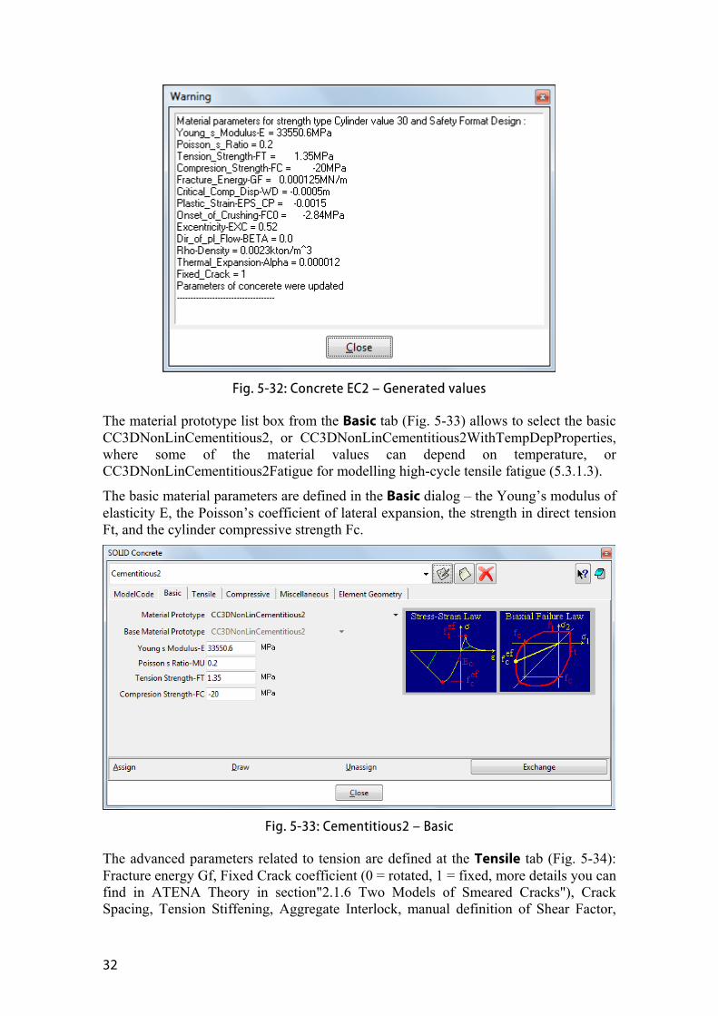
Fig. 5-32: Concrete EC2 – Generated values
The material prototype list box from the Basic tab (Fig. 5-33) allows to select the basic CC3DNonLinCementitious2, or CC3DNonLinCementitious2WithTempDepProperties, where some of the material values can depend on temperature, or CC3DNonLinCementitious2Fatigue for modelling high-cycle tensile fatigue (5.3.1.3).
The basic material parameters are defined in the Basic dialog – the Young’s modulus of elasticity E, the Poisson’s coefficient of lateral expansion, the strength in direct tension Ft, and the cylinder compressive strength Fc.
Fig. 5-33: Cementitious2 – Basic
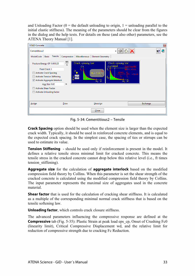
The advanced parameters related to tension are defined at the Tensile tab (Fig. 5-34): Fracture energy Gf, Fixed Crack coefficient (0 = rotated, 1 = fixed, more details you can find in ATENA Theory in section"2.1.6 Two Models of Smeared Cracks"), Crack Spacing, Tension Stiffening, Aggregate Interlock, manual definition of Shear Factor,
ATENA Science - GiD - User´s Manual 33
and Unloading Factor (0 = the default unloading to origin, 1 = unloading parallel to the initial elastic stiffness). The meaning of the parameters should be clear from the figures in the dialog and the help texts. For details on these (and also other) parameters, see the ATENA Theory Manual [1].
Fig. 5-34: Cementitious2 – Tensile
Crack Spacing option should be used when the element size is larger than the expected crack width. Typically, it should be used in reinforced concrete elements, and is equal to the expected crack spacing. In the simplest case, the spacing of ties or stirrups can be used to estimate its value.
Tension Stiffening - should be used only if reinforcement is present in the model. It defines a relative tensile stress minimal limit for cracked concrete. This means the tensile stress in the cracked concrete cannot drop below this relative level (i.e., ft times tension_stiffening).
Aggregate size for the calculation of aggregate interlock based on the modified compression field theory by Collins. When this parameter is set the shear strength of the cracked concrete is calculated using the modified compression field theory by Collins. The input parameter represents the maximal size of aggregates used in the concrete material.
Shear factor that is used for the calculation of cracking shear stiffness. It is calculated as a multiple of the corresponding minimal normal crack stiffness that is based on the tensile softening law.
Unloading factor, which controls crack closure stiffness.
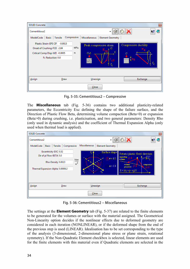
The advanced parameters influencing the compressive response are defined at the Compressive tab (Fig. 5-35): Plastic Strain at peak load eps_cp, Onset of Crushing Fc0 (linearity limit), Critical Compressive Displacement wd, and the relative limit for reduction of compressive strength due to cracking Fc Reduction.
34
Fig. 5-35: Cementitious2 – Compressive
The Miscellaneous tab (Fig. 5-36) contains two additional plasticity-related parameters, the Eccentricity Exc defining the shape of the failure surface, and the Direction of Plastic Flow Beta, determining volume compaction (Beta<0) or expansion (Beta>0) during crushing, i.e. plasticisation, and two general parameters: Density Rho (only used in dynamic analysis) and the coefficient of Thermal Expansion Alpha (only used when thermal load is applied).
Fig. 5-36: Cementitious2 – Miscellaneous
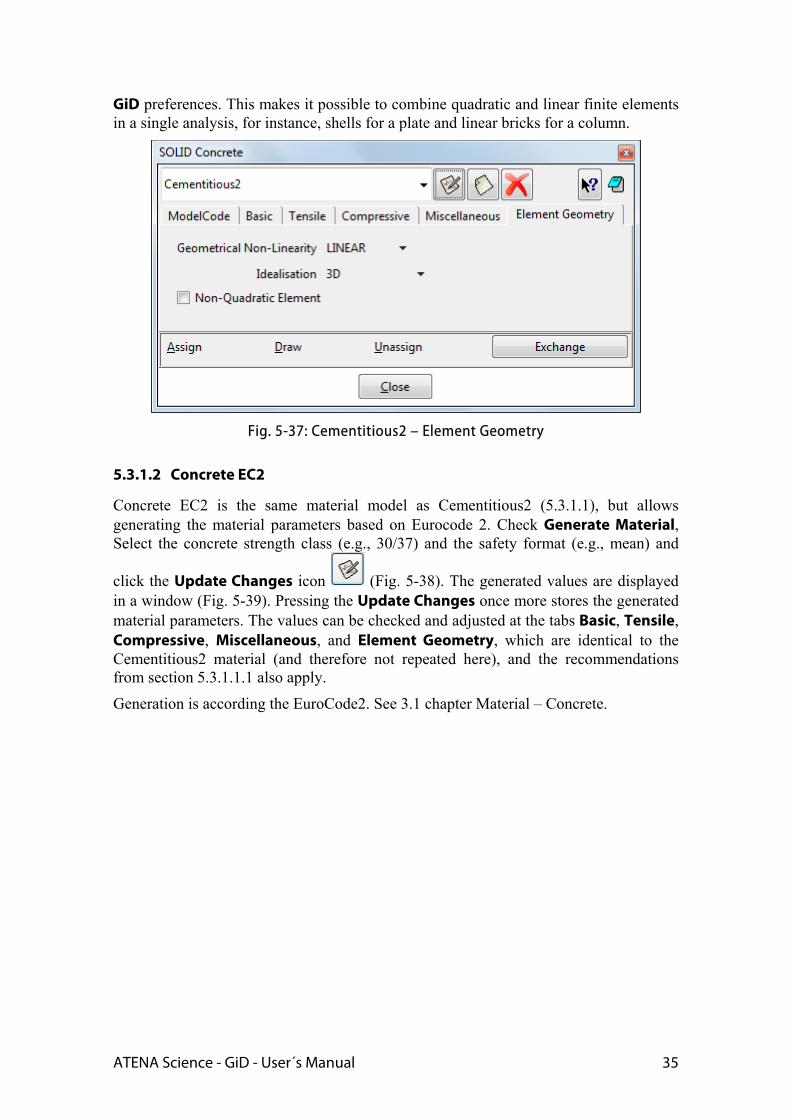
The settings at the Element Geometry tab (Fig. 5-37) are related to the finite elements to be generated for the volumes or surface with the material assigned. The Geometrical Non-Linearity option decides if the nonlinear effects due to deformed geometry are considered in each iteration (NONLINEAR), or if the deformed shape from the end of the previous step is used (LINEAR). Idealisation has to be set corresponding to the type of the analysis (3-dimensional, 2-dimensional plane stress or plane strain, rotational symmetry). If the Non-Quadratic Element checkbox is selected, linear elements are used for the finite elements with this material even if Quadratic elements are selected in the
ATENA Science - GiD - User´s Manual 35
GiD preferences. This makes it possible to combine quadratic and linear finite elements in a single analysis, for instance, shells for a plate and linear bricks for a column.
Fig. 5-37: Cementitious2 – Element Geometry
5.3.1.2 Concrete EC2
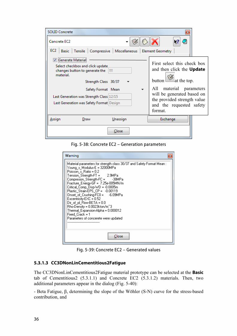
Concrete EC2 is the same material model as Cementitious2 (5.3.1.1), but allows generating the material parameters based on Eurocode 2. Check Generate Material, Select the concrete strength class (e.g., 30/37) and the safety format (e.g., mean) and
click the Update Changes icon (Fig. 5-38). The generated values are displayed in a window (Fig. 5-39). Pressing the Update Changes once more stores the generated material parameters. The values can be checked and adjusted at the tabs Basic, Tensile, Compressive, Miscellaneous, and Element Geometry, which are identical to the Cementitious2 material (and therefore not repeated here), and the recommendations from section 5.3.1.1.1 also apply.
Generation is according the EuroCode2. See 3.1 chapter Material – Concrete.
36
Fig. 5-38: Concrete EC2 – Generation parameters
Fig. 5-39: Concrete EC2 – Generated values
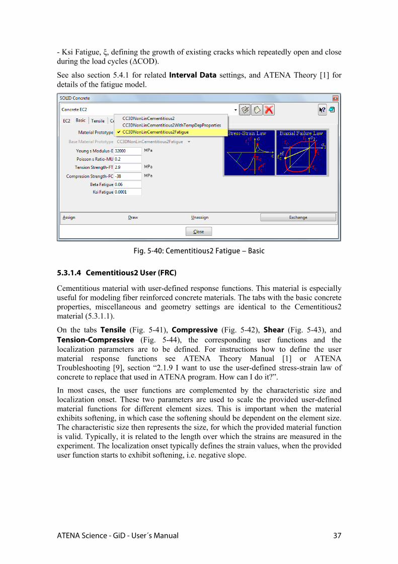
5.3.1.3 CC3DNonLinCementitious2Fatigue
The CC3DNonLinCementitious2Fatigue material prototype can be selected at the Basic tab of Cementitious2 (5.3.1.1) and Concrete EC2 (5.3.1.2) materials. Then, two additional parameters appear in the dialog (Fig. 5-40):
- Beta Fatigue, β, determining the slope of the Wöhler (S-N) curve for the stress-based contribution, and
First select this check box and then click the Update
button at the top.
All material parameters will be generated based on the provided strength value and the requested safety format.
ATENA Science - GiD - User´s Manual 37
- Ksi Fatigue, ξ, defining the growth of existing cracks which repeatedly open and close during the load cycles (ΔCOD).
See also section 5.4.1 for related Interval Data settings, and ATENA Theory [1] for details of the fatigue model.
Fig. 5-40: Cementitious2 Fatigue – Basic
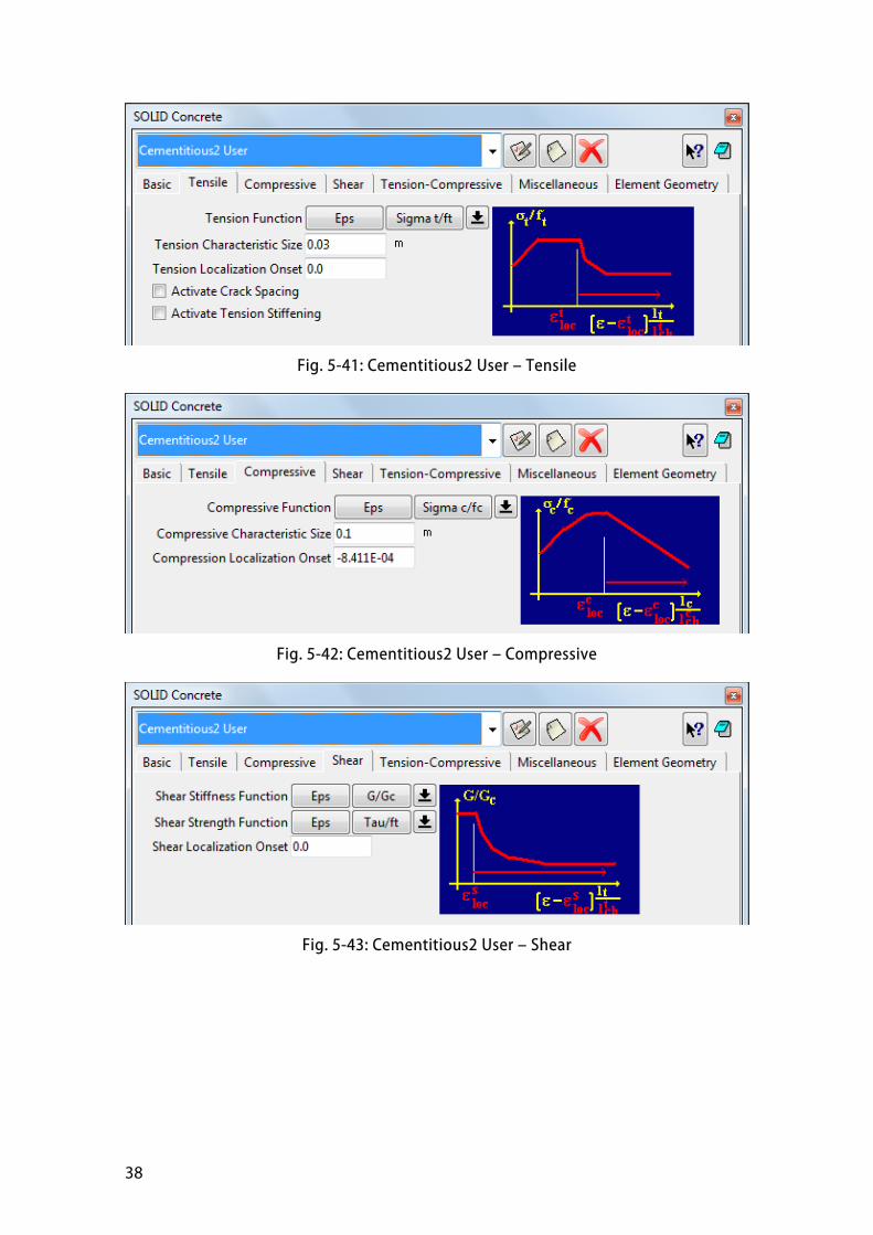
5.3.1.4 Cementitious2 User (FRC)
Cementitious material with user-defined response functions. This material is especially useful for modeling fiber reinforced concrete materials. The tabs with the basic concrete properties, miscellaneous and geometry settings are identical to the Cementitious2 material (5.3.1.1).
On the tabs Tensile (Fig. 5-41), Compressive (Fig. 5-42), Shear (Fig. 5-43), and Tension-Compressive (Fig. 5-44), the corresponding user functions and the localization parameters are to be defined. For instructions how to define the user material response functions see ATENA Theory Manual [1] or ATENA Troubleshooting [9], section “2.1.9 I want to use the user-defined stress-strain law of concrete to replace that used in ATENA program. How can I do it?”.
In most cases, the user functions are complemented by the characteristic size and localization onset. These two parameters are used to scale the provided user-defined material functions for different element sizes. This is important when the material exhibits softening, in which case the softening should be dependent on the element size. The characteristic size then represents the size, for which the provided material function is valid. Typically, it is related to the length over which the strains are measured in the experiment. The localization onset typically defines the strain values, when the provided user function starts to exhibit softening, i.e. negative slope.
38
Fig. 5-41: Cementitious2 User – Tensile
Fig. 5-42: Cementitious2 User – Compressive
Fig. 5-43: Cementitious2 User – Shear
ATENA Science - GiD - User´s Manual 39
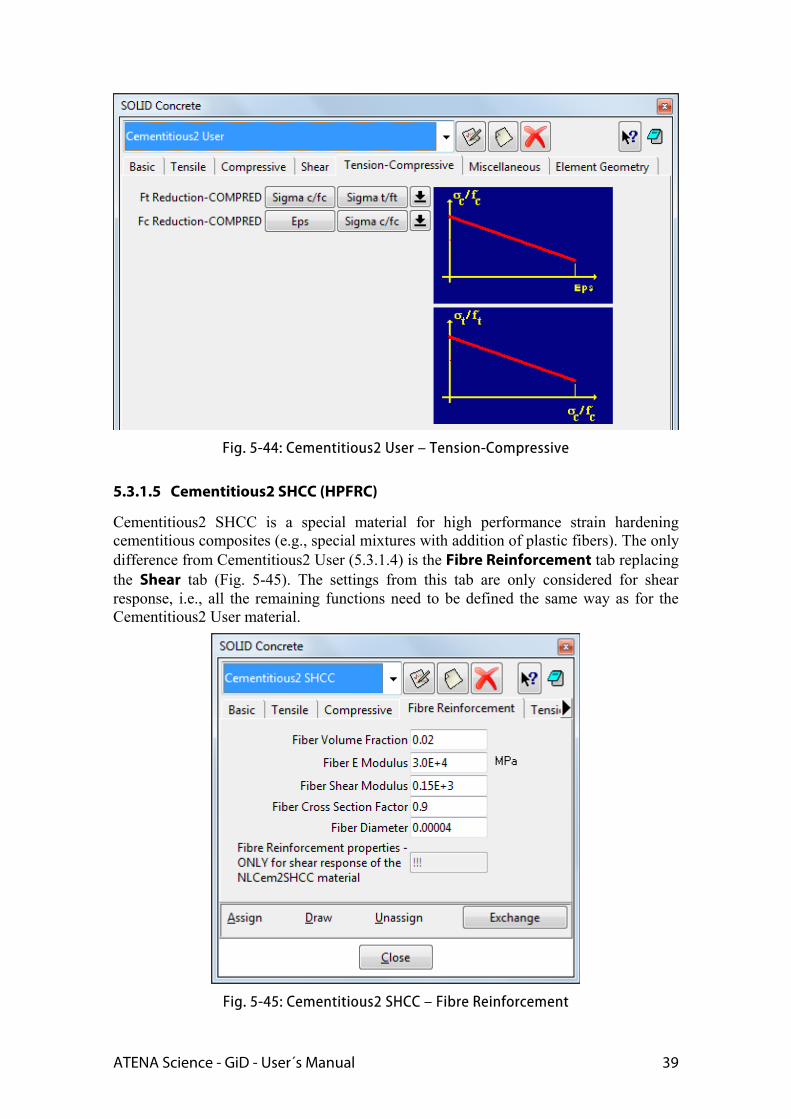
Fig. 5-44: Cementitious2 User – Tension-Compressive
5.3.1.5 Cementitious2 SHCC (HPFRC)
Cementitious2 SHCC is a special material for high performance strain hardening cementitious composites (e.g., special mixtures with addition of plastic fibers). The only difference from Cementitious2 User (5.3.1.4) is the Fibre Reinforcement tab replacing the Shear tab (Fig. 5-45). The settings from this tab are only considered for shear response, i.e., all the remaining functions need to be defined the same way as for the Cementitious2 User material.
Fig. 5-45: Cementitious2 SHCC – Fibre Reinforcement
40
5.3.2 Shell Material
In this section, shell material is described. In ATENA-GiD, this material has to be assigned to volumes where shell (plate) elements are to be used (unlike ATENA Engineering 3D, where one switches between volume and shell elements in Macroelement definition). Shell material has geometry which supports Ahmad elements (CCAhmadElement) and IsoBrick/IsoWedge elements (CCIsoShellBrick, CCIsoShellWedge). These elements are reduced from a quadratic 3D brick (wedge) element with 20 (15) nodes. The element has 9 (6) integration points in shell plane and layers in direction normal to its plane. The total number of integration points is 9x(number of layers) for the bricks, or 6x(number of layers) for the wedges.
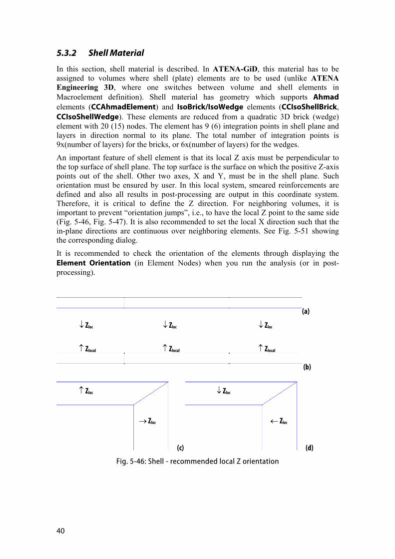
An important feature of shell element is that its local Z axis must be perpendicular to the top surface of shell plane. The top surface is the surface on which the positive Z-axis points out of the shell. Other two axes, X and Y, must be in the shell plane. Such orientation must be ensured by user. In this local system, smeared reinforcements are defined and also all results in post-processing are output in this coordinate system. Therefore, it is critical to define the Z direction. For neighboring volumes, it is important to prevent “orientation jumps”, i.e., to have the local Z point to the same side (Fig. 5-46, Fig. 5-47). It is also recommended to set the local X direction such that the in-plane directions are continuous over neighboring elements. See Fig. 5-51 showing the corresponding dialog.
It is recommended to check the orientation of the elements through displaying the Element Orientation (in Element Nodes) when you run the analysis (or in post-processing).
(a)
(b)
(c) (d)
Fig. 5-46: Shell - recommended local Z orientation
Zlocal Zlocal Zlocal
Zloc Zloc Zloc
Zloc Zloc
Zloc Zloc
ATENA Science - GiD - User´s Manual 41
(a) (b)
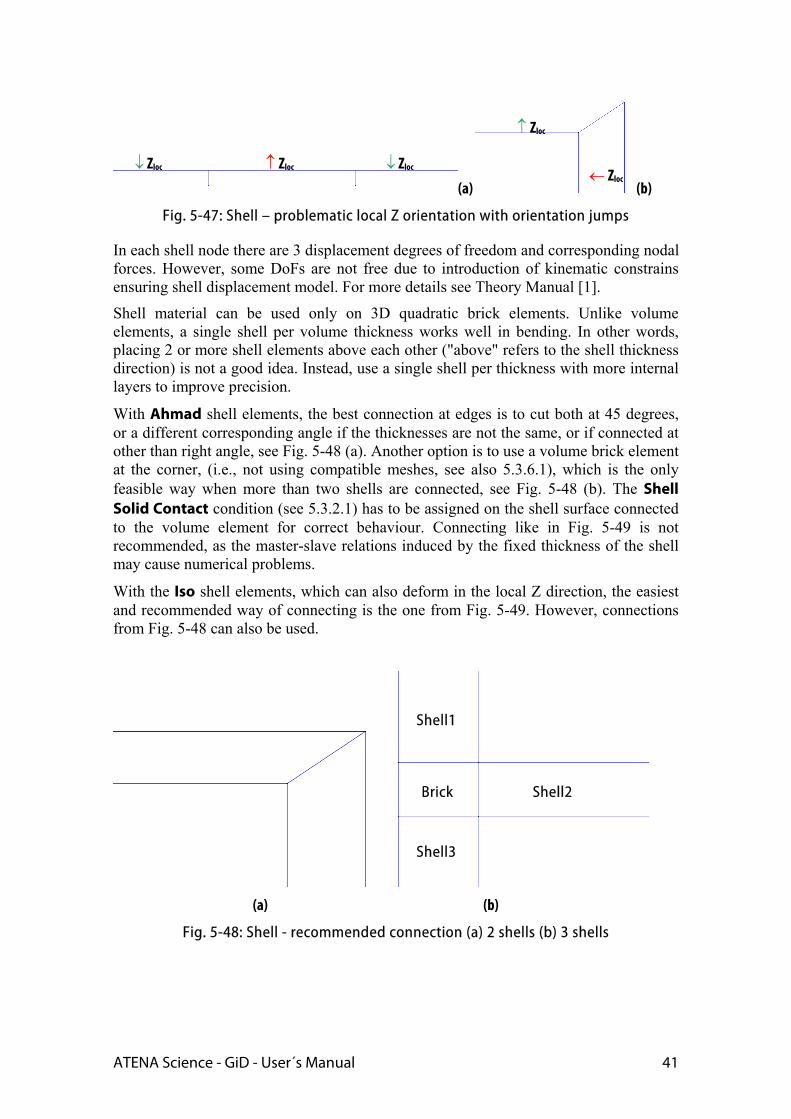
Fig. 5-47: Shell – problematic local Z orientation with orientation jumps
In each shell node there are 3 displacement degrees of freedom and corresponding nodal forces. However, some DoFs are not free due to introduction of kinematic constrains ensuring shell displacement model. For more details see Theory Manual [1].
Shell material can be used only on 3D quadratic brick elements. Unlike volume elements, a single shell per volume thickness works well in bending. In other words, placing 2 or more shell elements above each other ("above" refers to the shell thickness direction) is not a good idea. Instead, use a single shell per thickness with more internal layers to improve precision.
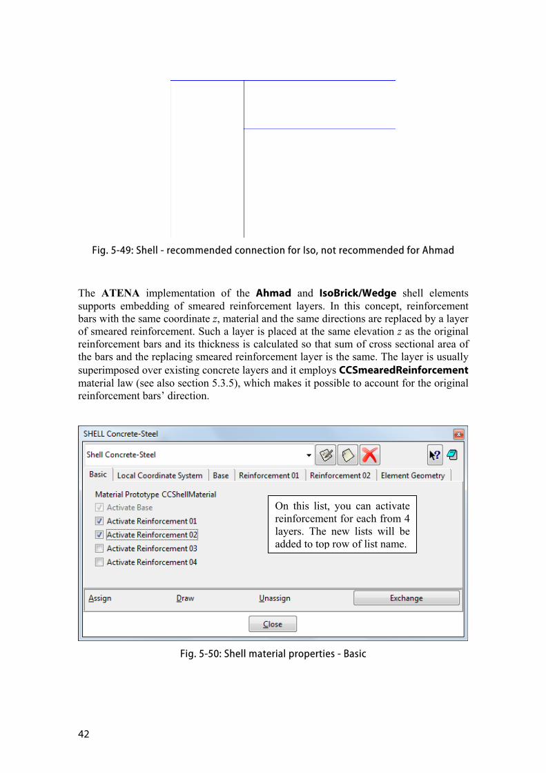
With Ahmad shell elements, the best connection at edges is to cut both at 45 degrees, or a different corresponding angle if the thicknesses are not the same, or if connected at other than right angle, see Fig. 5-48 (a). Another option is to use a volume brick element at the corner, (i.e., not using compatible meshes, see also 5.3.6.1), which is the only feasible way when more than two shells are connected, see Fig. 5-48 (b). The Shell Solid Contact condition (see 5.3.2.1) has to be assigned on the shell surface connected to the volume element for correct behaviour. Connecting like in Fig. 5-49 is not recommended, as the master-slave relations induced by the fixed thickness of the shell may cause numerical problems.
With the Iso shell elements, which can also deform in the local Z direction, the easiest and recommended way of connecting is the one from Fig. 5-49. However, connections from Fig. 5-48 can also be used.
(a) (b)
Fig. 5-48: Shell - recommended connection (a) 2 shells (b) 3 shells
Shell1
Brick Shell2
Shell3
Zloc Zloc Zloc
Zloc
Zloc
42
Fig. 5-49: Shell - recommended connection for Iso, not recommended for Ahmad
The ATENA implementation of the Ahmad and IsoBrick/Wedge shell elements supports embedding of smeared reinforcement layers. In this concept, reinforcement bars with the same coordinate z, material and the same directions are replaced by a layer of smeared reinforcement. Such a layer is placed at the same elevation z as the original reinforcement bars and its thickness is calculated so that sum of cross sectional area of the bars and the replacing smeared reinforcement layer is the same. The layer is usually superimposed over existing concrete layers and it employs CCSmearedReinforcement material law (see also section 5.3.5), which makes it possible to account for the original reinforcement bars’ direction.
Fig. 5-50: Shell material properties - Basic
On this list, you can activate reinforcement for each from 4 layers. The new lists will be added to top row of list name.
ATENA Science - GiD - User´s Manual 43
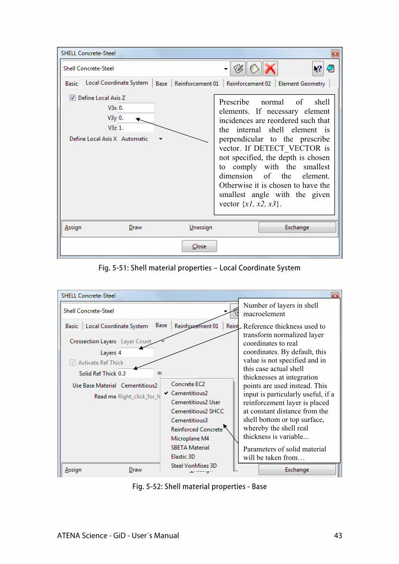
Fig. 5-51: Shell material properties – Local Coordinate System
Fig. 5-52: Shell material properties - Base
Prescribe normal of shell elements. If necessary element incidences are reordered such that the internal shell element is perpendicular to the prescribe vector. If DETECT_VECTOR is not specified, the depth is chosen to comply with the smallest dimension of the element. Otherwise it is chosen to have the smallest angle with the given vector {x1, x2, x3}.
Number of layers in shell macroelement
Reference thickness used to transform normalized layer coordinates to real coordinates. By default, this value is not specified and in this case actual shell thicknesses at integration points are used instead. This input is particularly useful, if a reinforcement layer is placed at constant distance from the shell bottom or top surface, whereby the shell real thickness is variable...
Parameters of solid material will be taken from…
44
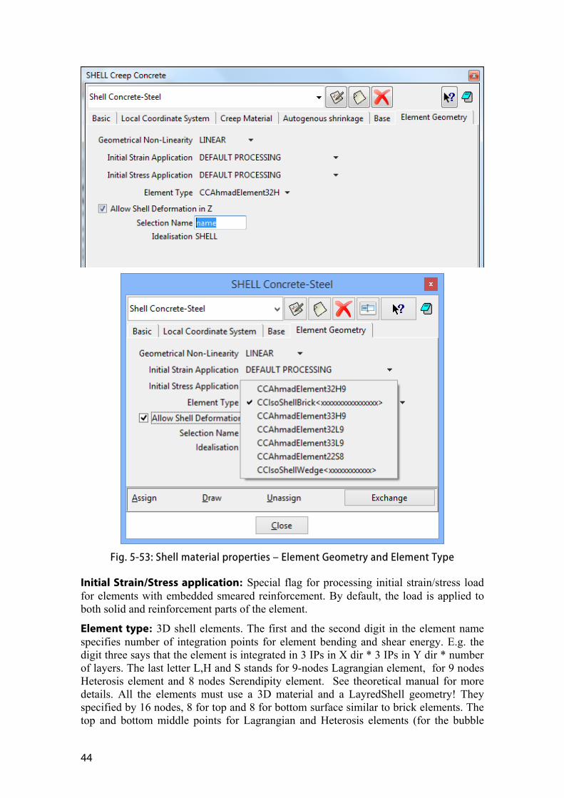
Fig. 5-53: Shell material properties – Element Geometry and Element Type
Initial Strain/Stress application: Special flag for processing initial strain/stress load for elements with embedded smeared reinforcement. By default, the load is applied to both solid and reinforcement parts of the element.
Element type: 3D shell elements. The first and the second digit in the element name specifies number of integration points for element bending and shear energy. E.g. the digit three says that the element is integrated in 3 IPs in X dir * 3 IPs in Y dir * number of layers. The last letter L,H and S stands for 9-nodes Lagrangian element, for 9 nodes Heterosis element and 8 nodes Serendipity element. See theoretical manual for more details. All the elements must use a 3D material and a LayredShell geometry! They specified by 16 nodes, 8 for top and 8 for bottom surface similar to brick elements. The top and bottom middle points for Lagrangian and Heterosis elements (for the bubble
ATENA Science - GiD - User´s Manual 45
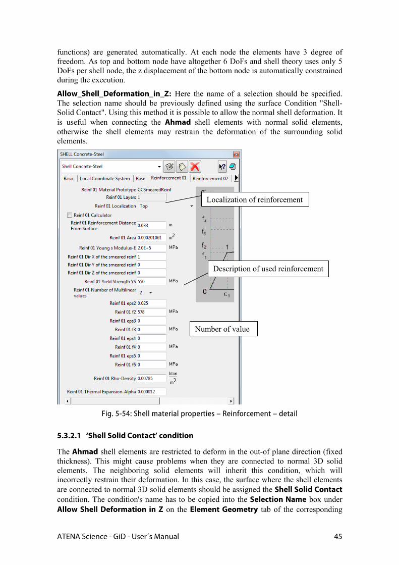
functions) are generated automatically. At each node the elements have 3 degree of freedom. As top and bottom node have altogether 6 DoFs and shell theory uses only 5 DoFs per shell node, the z displacement of the bottom node is automatically constrained during the execution.
Allow_Shell_Deformation_in_Z: Here the name of a selection should be specified. The selection name should be previously defined using the surface Condition "Shell-Solid Contact". Using this method it is possible to allow the normal shell deformation. It is useful when connecting the Ahmad shell elements with normal solid elements, otherwise the shell elements may restrain the deformation of the surrounding solid elements.
Fig. 5-54: Shell material properties – Reinforcement – detail
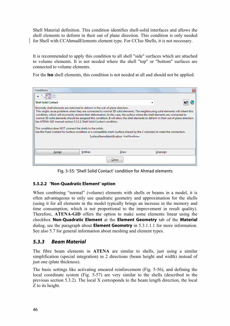
5.3.2.1 ‘Shell Solid Contact’ condition
The Ahmad shell elements are restricted to deform in the out-of plane direction (fixed thickness). This might cause problems when they are connected to normal 3D solid elements. The neighboring solid elements will inherit this condition, which will incorrectly restrain their deformation. In this case, the surface where the shell elements are connected to normal 3D solid elements should be assigned the Shell Solid Contact condition. The condition's name has to be copied into the Selection Name box under Allow Shell Deformation in Z on the Element Geometry tab of the corresponding
Localization of reinforcement
Description of used reinforcement
Number of value
46
Shell Material definition. This condition identifies shell-solid interfaces and allows the shell elements to deform in their out of plane direction. This condition is only needed for Shell with CCAhmadElements element type. For CCIso Shells, it is not necessary.
It is recommended to apply this condition to all shell "side" surfaces which are attached to volume elements. It is not needed where the shell "top" or "bottom" surfaces are connected to volume elements.
For the Iso shell elements, this condition is not needed at all and should not be applied.
Fig. 5-55: ‘Shell Solid Contact’ condition for Ahmad elements
5.3.2.2 ‘Non-Quadratic Element’ option
When combining “normal” (volume) elements with shells or beams in a model, it is often advantageous to only use quadratic geometry and approximation for the shells (using it for all elements in the model typically brings an increase in the memory and time consumption, which is not proportional to the improvement in result quality). Therefore, ATENA-GiD offers the option to make some elements linear using the checkbox Non-Quadratic Element at the Element Geometry tab of the Material dialog, see the paragraph about Element Geometry in 5.3.1.1.1 for more information. See also 5.7 for general information about meshing and element types.
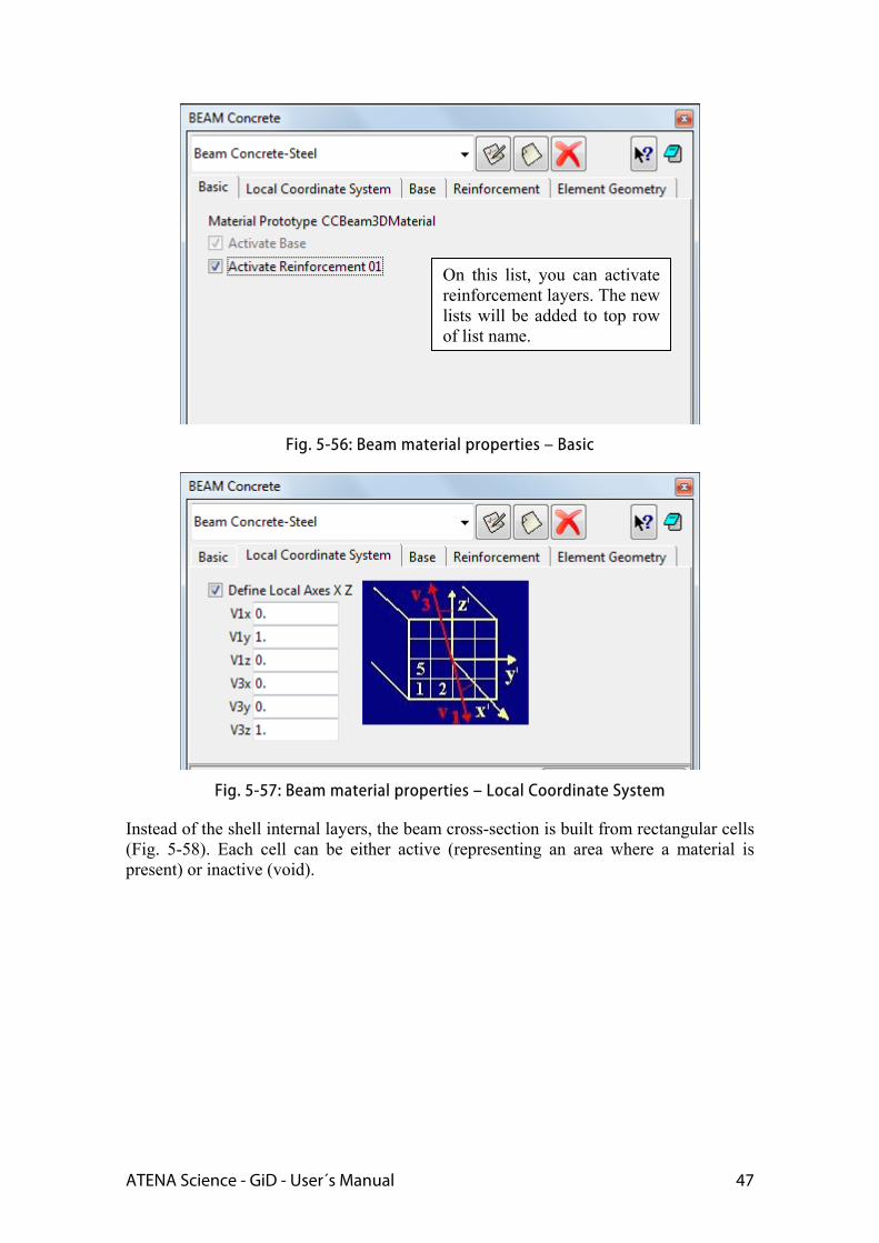
5.3.3 Beam Material
The fibre beam elements in ATENA are similar to shells, just using a similar simplification (special integration) in 2 directions (beam height and width) instead of just one (plate thickness).
The basic settings like activating smeared reinforcement (Fig. 5-56), and defining the local coordinate system (Fig. 5-57) are very similar to the shells (described in the previous section 5.3.2). The local X corresponds to the beam length direction, the local Z to its height.
ATENA Science - GiD - User´s Manual 47
Fig. 5-56: Beam material properties – Basic
Fig. 5-57: Beam material properties – Local Coordinate System
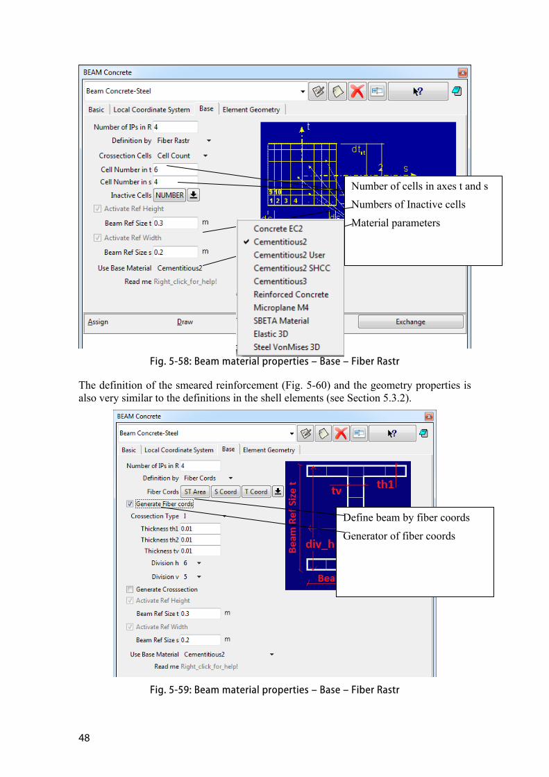
Instead of the shell internal layers, the beam cross-section is built from rectangular cells (Fig. 5-58). Each cell can be either active (representing an area where a material is present) or inactive (void).
On this list, you can activate reinforcement layers. The new lists will be added to top row of list name.
48
Fig. 5-58: Beam material properties – Base – Fiber Rastr
The definition of the smeared reinforcement (Fig. 5-60) and the geometry properties is also very similar to the definitions in the shell elements (see Section 5.3.2).
Fig. 5-59: Beam material properties – Base – Fiber Rastr
Number of cells in axes t and s
Numbers of Inactive cells
Material parameters
Define beam by fiber coords
Generator of fiber coords
ATENA Science - GiD - User´s Manual 49
Fig. 5-60: Beam material properties – Reinforcement
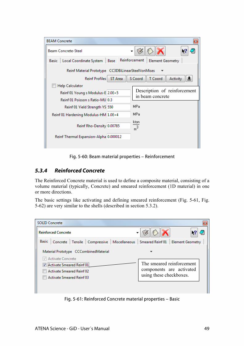
5.3.4 Reinforced Concrete
The Reinforced Concrete material is used to define a composite material, consisting of a volume material (typically, Concrete) and smeared reinforcement (1D material) in one or more directions.
The basic settings like activating and defining smeared reinforcement (Fig. 5-61, Fig. 5-62) are very similar to the shells (described in section 5.3.2).
Fig. 5-61: Reinforced Concrete material properties – Basic
The smeared reinforcement components are activated using these checkboxes.
Description of reinforcement in beam concrete
50
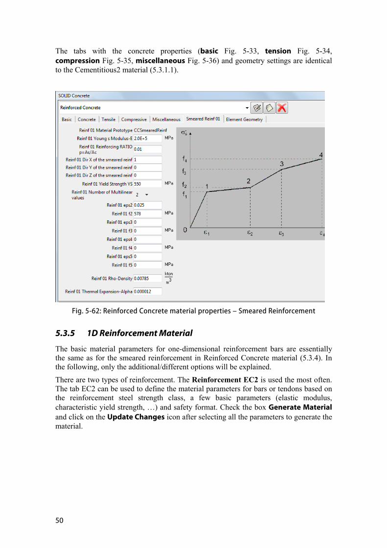
The tabs with the concrete properties (basic Fig. 5-33, tension Fig. 5-34, compression Fig. 5-35, miscellaneous Fig. 5-36) and geometry settings are identical to the Cementitious2 material (5.3.1.1).
Fig. 5-62: Reinforced Concrete material properties – Smeared Reinforcement
5.3.5 1D Reinforcement Material
The basic material parameters for one-dimensional reinforcement bars are essentially the same as for the smeared reinforcement in Reinforced Concrete material (5.3.4). In the following, only the additional/different options will be explained.
There are two types of reinforcement. The Reinforcement EC2 is used the most often. The tab EC2 can be used to define the material parameters for bars or tendons based on the reinforcement steel strength class, a few basic parameters (elastic modulus, characteristic yield strength, …) and safety format. Check the box Generate Material and click on the Update Changes icon after selecting all the parameters to generate the material.
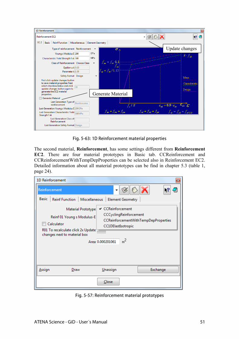
ATENA Science - GiD - User´s Manual 51
Fig. 5-63: 1D Reinforcement material properties
The second material, Reinforcement, has some settings different from Reinforcement EC2. There are four material prototypes in Basic tab. CCReinforcement and CCReinforcementWithTempDepProperties can be selected also in Reinforcement EC2. Detailed information about all material prototypes can be find in chapter 5.3 (table 1, page 24).
Fig. 5-57: Reinforcement material prototypes
Generate Material
Update changes
52
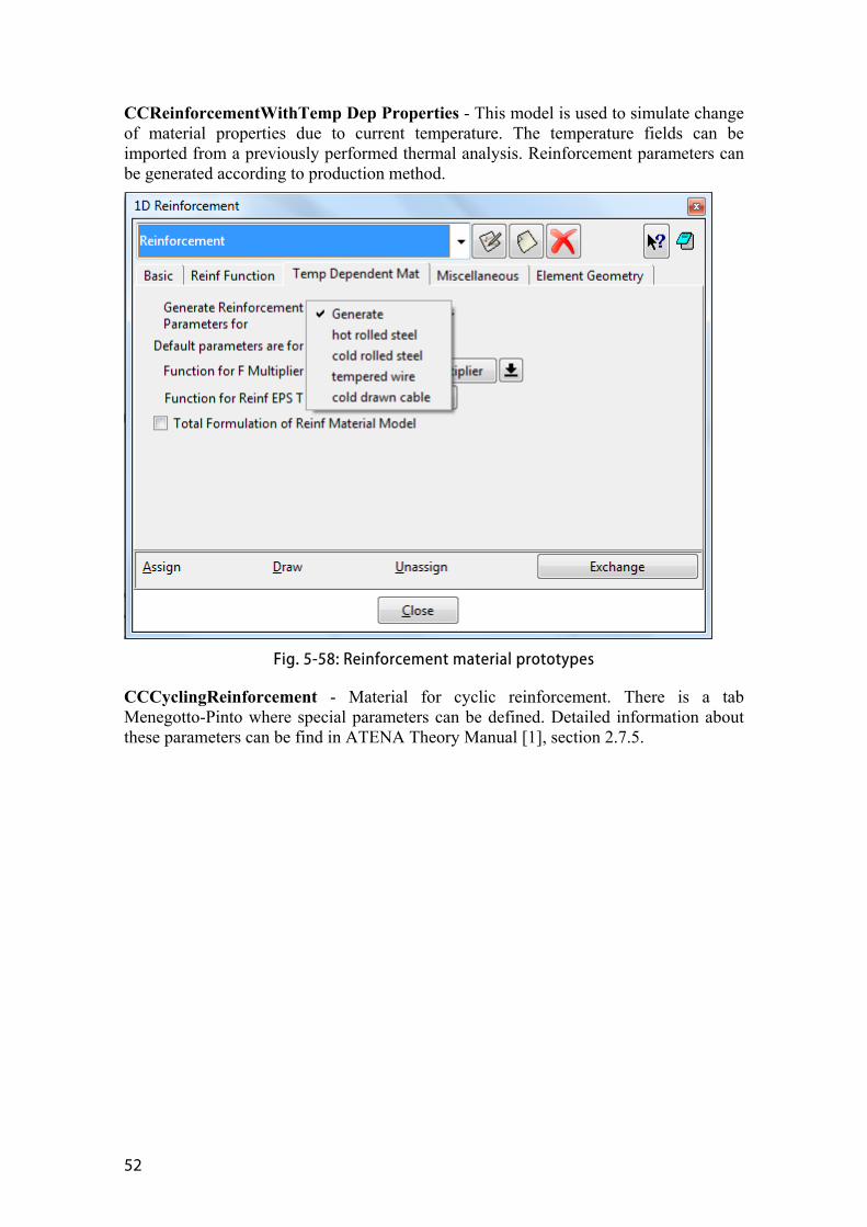
CCReinforcementWithTemp Dep Properties - This model is used to simulate change of material properties due to current temperature. The temperature fields can be imported from a previously performed thermal analysis. Reinforcement parameters can be generated according to production method.
Fig. 5-58: Reinforcement material prototypes
CCCyclingReinforcement - Material for cyclic reinforcement. There is a tab Menegotto-Pinto where special parameters can be defined. Detailed information about these parameters can be find in ATENA Theory Manual [1], section 2.7.5.
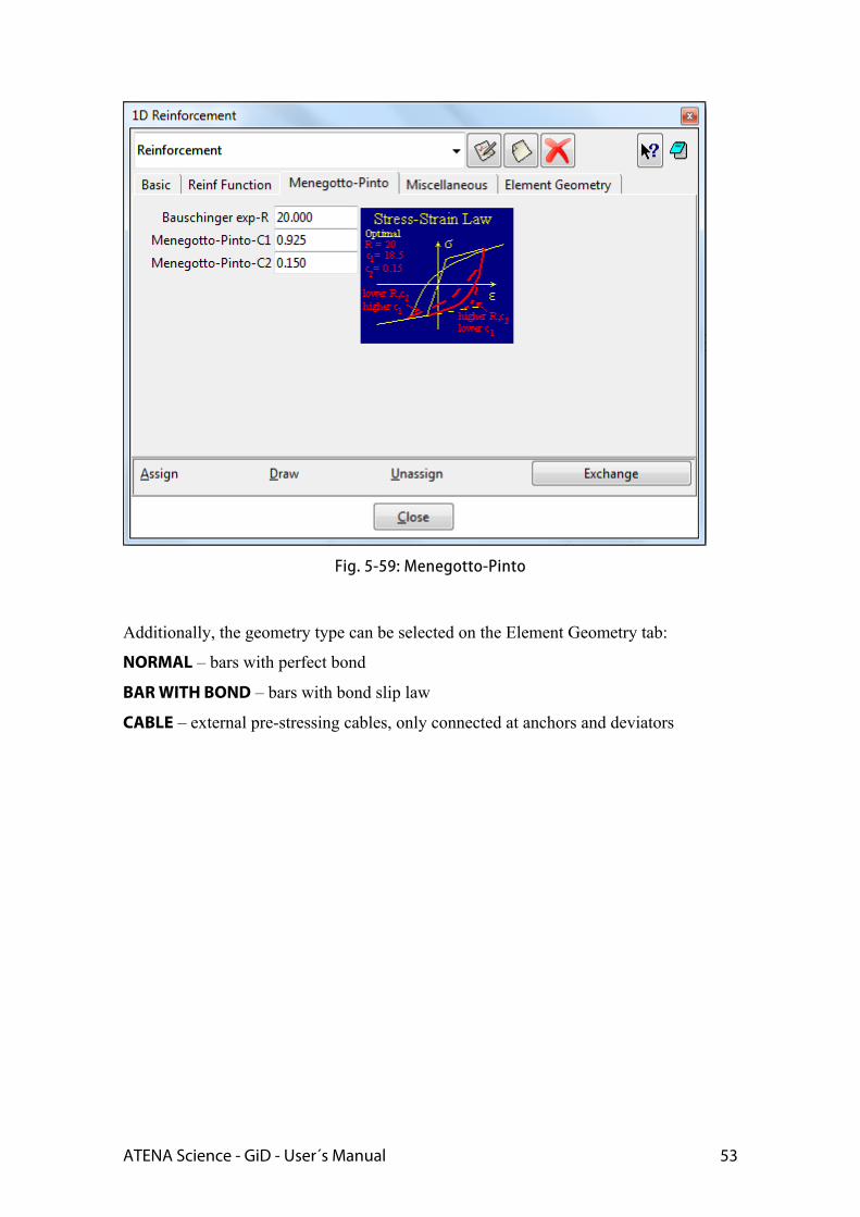
ATENA Science - GiD - User´s Manual 53
Fig. 5-59: Menegotto-Pinto
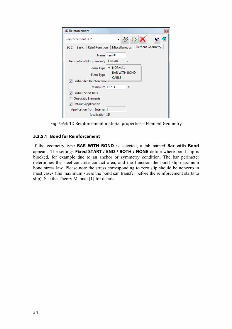
Additionally, the geometry type can be selected on the Element Geometry tab:
NORMAL – bars with perfect bond
BAR WITH BOND – bars with bond slip law
CABLE – external pre-stressing cables, only connected at anchors and deviators
54
Fig. 5-64: 1D Reinforcement material properties – Element Geometry
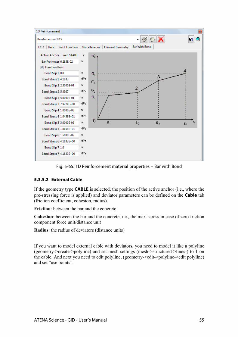
5.3.5.1 Bond for Reinforcement
If the geometry type BAR WITH BOND is selected, a tab named Bar with Bond appears. The settings Fixed START / END / BOTH / NONE define where bond slip is blocked, for example due to an anchor or symmetry condition. The bar perimeter determines the steel-concrete contact area, and the function the bond slip-maximum bond stress law. Please note the stress corresponding to zero slip should be nonzero in most cases (the maximum stress the bond can transfer before the reinforcement starts to slip). See the Theory Manual [1] for details.
ATENA Science - GiD - User´s Manual 55
Fig. 5-65: 1D Reinforcement material properties – Bar with Bond
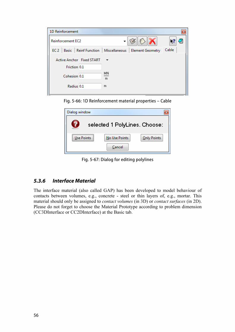
5.3.5.2 External Cable
If the geometry type CABLE is selected, the position of the active anchor (i.e., where the pre-stressing force is applied) and deviator parameters can be defined on the Cable tab (friction coefficient, cohesion, radius).
Friction: between the bar and the concrete
Cohesion: between the bar and the concrete, i.e., the max. stress in case of zero friction component force unit/distance unit
Radius: the radius of deviators (distance units)
If you want to model external cable with deviators, you need to model it like a polyline (geometry->create->polyline) and set mesh settings (mesh->structured->lines-) to 1 on the cable. And next you need to edit polyline, (geometry->edit->polyline->edit polyline) and set “use points”.
56
Fig. 5-66: 1D Reinforcement material properties – Cable
Fig. 5-67: Dialog for editing polylines
5.3.6 Interface Material
The interface material (also called GAP) has been developed to model behaviour of contacts between volumes, e.g., concrete - steel or thin layers of, e.g., mortar. This material should only be assigned to contact volumes (in 3D) or contact surfaces (in 2D). Please do not forget to choose the Material Prototype according to problem dimension (CC3DInterface or CC2DInterface) at the Basic tab.