atiner's conference paper series fos2018- 2507 · 2018-08-28 · atiner conference paper...

ATINER CONFERENCE PAPER SERIES No: LNG2014-1176

1

Athens Institute for Education and Research

ATINER

ATINER's Conference Paper Series

FOS2018- 2507

Patrizio Vanella

Research Associate

Gottfried Wilhelm Leibniz University Hannover

Germany

Stochastic Forecasting of Demographic Components

Based on Principal Component Analyses

ATINER CONFERENCE PAPER SERIES No: FOS2018-2507

2

An Introduction to

ATINER's Conference Paper Series

Conference papers are research/policy papers written and presented by academics at one

of ATINER‟s academic events. ATINER‟s association started to publish this conference

paper series in 2012. All published conference papers go through an initial peer review

aiming at disseminating and improving the ideas expressed in each work. Authors

welcome comments.

Dr. Gregory T. Papanikos

President


This paper should be cited as follows:

Vanella, P. (2018). “Stochastic Forecasting of Demographic Components

Based on Principal Component Analyses”, Athens: ATINER'S Conference

Paper Series, No: FOS20182507.


8 Valaoritou Street, Kolonaki, 10671 Athens, Greece

Tel: + 30 210 3634210 Fax: + 30 210 3634209 Email: [email protected] URL:

www.atiner.gr

URL Conference Papers Series: www.atiner.gr/papers.htm

Printed in Athens, Greece by the Athens Institute for Education and Research. All rights

reserved. Reproduction is allowed for non-commercial purposes if the source is fully

acknowledged.

ISSN: 2241-2891

28/08/2018


3

Stochastic Forecasting of Demographic Components Based on Principal

Component Analyses

Patrizio Vanella

Abstract

Adequate forecasts of future population developments that are based on cohort-

component methods demand an age- and sex-specific analysis; otherwise, the

structure of the future population cannot be specified correctly. Age-specific

demographic measures are both highly correlated and highly dimensional. Thus, a

methodology that not only considers the correlations between the random variables

but also reduces the effective dimensionality of the forecasting problem is needed:

principal component analysis serves both purposes simultaneously. This study

presents principal component analysis, from a mathematical-statistical perspective, to

users from the field of population studies. Furthermore, important aspects of time

series analysis, which are vital for an accurate stochastic forecast, are explained. The

application is illustrated via the simultaneous projection of selected age- and sex-

specific survival rates with projection intervals for Germany, Italy, Austria, and

Switzerland.

Keywords: Forecasting, Multivariate Methods, Principal Component Analysis,

Quantitative Population Studies, Time Series Analysis.


4

Introduction and Motivation

Official population projections are commonly conducted on the basis of

deterministic cohort-component models (Alho, 1990; Pötzsch and Rößger, 2015).

Stochastic forecasts are favorable compared to deterministic approaches (Keilman

and Pham, 2000) since, in addition to the most probable scenario, they identify

and quantify with respective probabilities infinitely many possible scenarios.

Stochastic models may also be based on the components of fertility, migration and

mortality. Autocorrelation and cross-correlation must be considered in future

forecasts because there are correlations between the different age groups and

genders as well as between observations at different points in the time series.

Therefore, this paper first presents a short introduction to principal component

analysis (PCA), where the focus is on explaining its use and a short illustration of

its functionality.

Moreover, important concepts of time series analysis (TSA) are considered,

with the explanation restricted to the aspects that are required for practical

applications, with no claim on completeness in mind. This contribution therefore

may be understood as a guide for statistical offices or demographic research

institutes; the concrete projections serve only illustrative purposes and should not

be mistaken as actual forecasts for future development. The methods are not

restricted to population studies; forecasters from various disciplines might find

this contribution interesting reading material. The explanation of the method is the

focal point of the paper, especially the implementation of the illustrated statistical

concepts of modeling and forecasting the components of demographic developments.

The method is demonstrated by simulating selected age- and sex-specific survival

rates (ASSSRs) for Germany, Italy, Austria, and Switzerland, but the model could

be applied to other countries or regions as well. Application to other problems in

demography or in other fields is not shown but may be done in principle the same

way it is presented in this contribution.

Introduction to Principal Component Analysis

Detailed population forecasts by sex and age show a high degree of

dimensionality, since for two genders up to 116 age groups should be investigated

(see Vanella, 2017). Moreover, these quantities are highly correlated with each

other. Forecasters have to address these two problems with appropriate methods.

PCA is recommended because it simultaneously addresses both problems. PCA

was originally developed by Pearson (1901) geometrically and involves applying

an orthogonal transformation to the original variables into the same number of

new, uncorrelated variables, which are labeled principal components (PCs). The

method is especially well suited for situations in which no causal relationship

between the variables is quantified, as is the case for regression analyses. Therefore,

PCA is especially appropriate for forecasting age- and sex-specific measures in a

demographic context. Each PC is a linear combination of N original variables. Let


5

be the ith

ASSSR in period t. Then, the jth

PC in the same period is

calculated by the following (Chatfield and Collins, 1980):

(1)

where can be interpreted as a correlation coefficient between the ith

ASSSR

and the jth

PC in period t.

Within the PCA framework, the PCs are deduced in decreasing order of the

magnitude of the total variance they explain. This means the first PC explains the

largest share of the variance in the original variables. Through the transformation,

a complex system with many variables can effectively be reduced to few

dimensions since the first few PCs explain the majority of the variance.

The first principal component (PC 1) is chosen to explain as much of the

variance as possible. Statistically, this means that the coefficients (or loadings, as

they are also called in this context) of the first linear combination are adjusted to

maximize the amount of covariance in the original variables that is explained. The

calculation is now illustrated with ASSSRs. For simplicity, the loadings are

assumed to be invariant through time;1 thus the index t is omitted. Given the

covariance matrix of S (the matrix of all ASSSRs), labeled , the variance of PC 1

is given by equation (2):

. (2)

The vector can be chosen arbitrarily. To reach a unique solution of the

maximization problem, a restriction for the elements of (also called the

eigenvector) must be stated. Normalizing to a length of one ensures an orthogonal

transformation. A vector has length one if its scalar product with itself is one (Handl,

2010):

. (3)

Due to the method of Lagrange multipliers, the stationary points2 of a function

under condition can be identified through the identification of the

stationary points of the affiliated Lagrange function . The Lagrangiana is

defined as follows:

(4)

Therefore, the maximization problem for the variance can be solved by

finding the stationary point of the following Lagrange function:

1Hyndman and Ullah (2007) have proposed a different approach with variable loadings.

2Those might be either local minima, maxima or saddle points.


6

. (5)

Accordingly, the stationary point is determined as follows:

(6)

Here, I is an identity matrix, which for consisting of p elements with

dimensions becomes the following:

. (7)

The first equation in (6) indicates that the matrix on the left-hand side of the

equation must be singular. Since must not be a null vector, guaranteeing a

nontrivial solution, it follows that the determinant of the matrix has to

equal zero (Chatfield and Collins, 1980):

. (8)

This is illustrated with a practical example. From age- and sex-specific data

on deaths and the end-of-year population, provided by the federal statistical

offices of Germany, Italy, and Austria and complemented by downloads from the

Human Mortality Database and the Eurostat Database, the ASSSRs for Germany,

Italy, Austria, and Switzerland are calculated for the years 1952-2016 (Destatis,

2005, 2015a, 2015b, 2015c, 2016, 2017a, 2017b, 2018a, 2018b; Eurostat, 2018;

Human Mortality Database, 2018a, 2018b, 2018c, 2018d; Istat, 2018a, 2018b,

2018c, 2018d, 2018e, 2018f; STATcube, 2018). For illustration, PCA is

performed on the covariance matrix of the logit transformed ASSSRs of 25-year-

old (cohort based) males for the four mentioned countries for the years 1952-

2016. Survival rates can only take values greater than zero and less than one, so

their projections are made through simulation of their logits. A logistic

transformation of an ASSSR s can be calculated as follows (Johnson, 1949):

(9)

The transformation leads to new unrestricted variables, whereas the

underlying ASSSRs cannot take simulation values outside the open interval (0,1)

in the forecast. After simulation, the results must be transformed back through the

inverse logit to obtain the final ASSSR trajectories.

The solutions of the optimization problem in this case are approximately

, and , which are also called the

eigenvalues (EWs) of the covariance matrix. The sum of the EWs is equal to the


7

sum of the covariance of the original variables; therefore, the EWs are sorted in

decreasing order. As mentioned earlier, one of the two reasons to apply PCA is to

reduce the original statistical problem into a small number of variables that

explain as much of the covariance in the original variables as possible. This means

the first eigenvalue (EW) represents the variance that is explained by PC 1.

Therefore, we can derive that PC 1 explains approximately 92.4% of the overall

covariance of the four time series (TS), whereas PC 1 and PC 2 already explain

over 97%.

Plugging the EWs into (6) individually leads to the respective EVs, e.g., EV 1:

PC 1 is negatively loaded with all of the four logit-ASSSRs, therefore indicating

a type of general mortality index, similar to the Lee-Carter index (Lee and Carter,

1992). The associated PCs can be easily derived by (1).

One important question is the determination of the number of PCs for the

analysis. There is no trivial answer; the determination of the number of PCs to use

is subjective. Nevertheless, criteria have been proposed to simplify the decision.

One possibility is to define a minimum percentage of the variation to be

explained. If we would, e.g., target covering at least 95% of the variance in the

ASSSRs, we would take the first two PCs into our model. Another common

method to select the number of PCs is graphically analyzing the EVs of the

covariance matrix with a scree plot (see Handl, 2010), as shown in Figure 1.


8

Figure 1. Scree Plot for the Principal Components

Only the PCs that lie on the left-hand side of the elbow are included in the

model; moreover, there is no clear consensus whether the PC at the elbow itself

should be included as well. In this case, the scree plot suggests one or two PCs. From

a practitioner‟s point of view, it is generally worthwhile to include the PC at the

elbow when making forecasts; otherwise, in many cases, a relatively large share of

the variance would be ignored, leading to biased results when constructing prediction

intervals (PIs). This result can be observed in many practical applications. Vanella

(2017) proposed a simulation method that includes the uncertainty arising from

omitting most of the PCs to prevent excessively narrow forecast PIs. This topic is not

considered further in this paper.3 Kaiser‟s and Jolliffe‟s criteria are additional

alternatives. Kaiser‟s criterion suggests using only PCs with EWs that are larger than

the mean EW (Handl, 2010). Jolliffe (2002) proposed 70% of the mean as the lower

limit. Nevertheless, the choice of criterion is subjective.

The focus of this section was the general description of PCA in a semimanual

practical application for a better understanding of the method. Nevertheless, PCA can

be performed relatively easily using R4.

3For further reading on this issue, see the aforementioned article.

4The standard commands prcomp and princomp, which are pre-installed, can be used for this.


9

Main Features of Time Series Analysis

In the section, some aspects of TSA, which are highly relevant in the context of

PC forecasting, will be explained.

A TS is a variable that generates one observation in each period. The

fundamental concept of modern TSA is stationarity, which will be explained briefly.

The TS of the ASSSR (in period t) of the 25-year-old males in Germany is defined as

. Stationarity (also called weak stationarity in the literature) is sufficiently defined

by two conditions: mean stationarity and auto covariance stationarity (Shumway and

Stoffer, 2011). The mean stationarity is defined by the equality of the TS mean in

each period:

. (10)

Autocovariance stationarity means the theoretical auto covariance between

two observations of the TS does not depend on the point in time but on the length

of the time interval separating the two observations:

(11)

Autoregressive integrated moving average (ARIMA) models, developed by

Box and Jenkins (Box et al., 2016), are of major importance for practical

applications, as subsequently explained (Shumway and Stoffer, 2011). A moving

average of order q (MA(q)) is defined as

(12)

where is a stochastic nuisance parameter in period t, which in practical

applications, is normally assumed to follow a Gaussian5 distribution with a mean

of zero and a variance :

. (13)

The stationarity assumption is beneficial because stationarity allows the

assumption that the nuisance parameter is identically distributed in each period. This

assumption is especially helpful for running simulations. An MA(q) model thus starts

from the premise that the current observation of the variables emerges exclusively as

a weighted sum of the last q manifestations of the nuisance parameter and the error in

the current period. In this notation, is the correlation coefficient of the TS with

respect to the error in period . is restricted between -1 and 1:

. (14)

5An alternative is to assume a Student‟s t-distributed nuisance parameter, as proposed by Raftery

et al. (2014).


10

A feasible alternate representation for an MA(q) process is the lag notation,

where L is the so-called lag operator6. The lag notation for an MA(q) process is as

follows:

(15)

The exponent of L indicates which past period is being considered. For

example, signifies .7

Another common type of TS model is an autoregressive model of order p

(AR(p)):

(16)

or in lag notation:

(17)

In an AR(p) model, the TS in period t is regressed on its previous p

observations (taking the error in period t into account). In this case,

. Similar to the MA(q) model,

. (18)

AR and MA models can also be combined; the combination of an AR(p)

model and an MA(q) model produces an ARMA(p,q) model, which is formally

defined as follows:

(19)

or

(20)

6Alternatively, some authors write about the backshift operator, which is the same.

7In practical applications, one has to be careful about the explicit definition of the coefficients. Some

statistical packages give a slightly different output, e.g., the output in R changes the sign of the

coefficient relative to this contribution.


11

As mentioned previously, the stationarity assumption is fundamental for

ARMA processes. The question is how to identify whether a TS is stationary;

graphical analysis is recommended as the first step in the investigation. Figure 2

illustrates a simulated stationary TS8.

Figure 2. Stationary Time Series

It is clear that neither the mean nor the variance show trending behavior.

Furthermore, the stationarity hypothesis should be confirmed using statistical

tests, such as the augmented Dickey-Fuller (ADF) test and the Kwiatkowski-

Phillips-Schmidt-Shin (KPSS) test. The standard ADF test checks the null

hypothesis, i.e., whether for the following equation

(21)

the condition

8The TS is generated by 1,000 computer simulations of a Gaussian random variable.


12

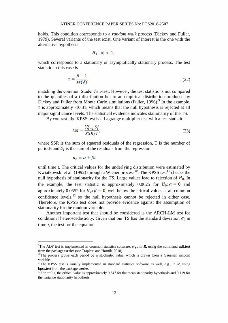
holds. This condition corresponds to a random walk process (Dickey and Fuller,

1979). Several variants of the test exist. One variant of interest is the one with the

alternative hypothesis

,

which corresponds to a stationary or asymptotically stationary process. The test

statistic in this case is

(22)

matching the common Student‟s t-test. However, the test statistic is not compared

to the quantiles of a t-distribution but to an empirical distribution produced by

Dickey and Fuller from Monte Carlo simulations (Fuller, 1996).9 In the example,

is approximately -10.31, which means that the null hypothesis is rejected at all

major significance levels. The statistical evidence indicates stationarity of the TS.

By contrast, the KPSS test is a Lagrange multiplier test with a test statistic

(23)

where SSR is the sum of squared residuals of the regression, T is the number of

periods and is the sum of the residuals from the regression

until time t. The critical values for the underlying distribution were estimated by

Kwiatkowski et al. (1992) through a Wiener process10

. The KPSS test11

checks the

null hypothesis of stationarity for the TS. Large values lead to rejection of . In

the example, the test statistic is approximately 0.0625 for and

approximately 0.0552 for , well below the critical values at all common

confidence levels,12

so the null hypothesis cannot be rejected in either case.

Therefore, the KPSS test does not provide evidence against the assumption of

stationarity for the random variable.

Another important test that should be considered is the ARCH-LM test for

conditional heteroscedasticity. Given that our TS has the standard deviation in

time t, the test for the equation

9The ADF test is implemented in common statistics software, e.g., in R, using the command adf.test

from the package tseries (see Trapletti and Hornik, 2018). 10

The process grows each period by a stochastic value, which is drawn from a Gaussian random

variable. 11

The KPSS test is usually implemented in standard statistics software as well, e.g., in R, using

kpss.test from the package tseries. 12

For α=0.1, the critical value is approximately 0.347 for the mean stationarity hypothesis and 0.119 for

the variance stationarity hypothesis.


13

checks the null hypothesis

where is some constant. If cannot be rejected, we find no evidence for

heteroscedasticity in the TS13

(Engle, 1982).

If the modeler concludes nonstationarity in the TS based on the statistical

tests, a transformation is needed. In this case, it is commonly assumed that the TS

was integrated, which is represented by the middle part of the ARIMA notation. A

d-times-integrated TS in the simplest case is denoted as an ARIMA(0,d,0) process

(Shumway and Stoffer, 2011):

(24)

In principle, a nonstationary TS can be transformed into a stationary TS by

differentiating it one or more times (Shumway und Stoffer, 2011). The first

difference of a TS is calculated as follows:

(25)

As known from calculus, this operation asymptotically leads to a reduction of

the power of the target function (here: the TS) by one. Figure 3 illustrates the

result of the differentiation by visualizing the TS of the logit-ASSSR of 25-year-

old males in Germany with its first and second difference for the time horizon

1952-2016.

13

The ARCH-LM Test should be implemented in common statistics software as well, i.e., it can be

applied easily by ArchTest, included in the package FinTS (Graves, 2013).


14

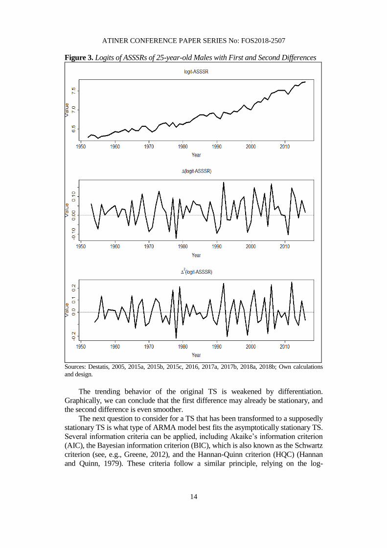
Figure 3. Logits of ASSSRs of 25-year-old Males with First and Second Differences

Sources: Destatis, 2005, 2015a, 2015b, 2015c, 2016, 2017a, 2017b, 2018a, 2018b; Own calculations

and design.

The trending behavior of the original TS is weakened by differentiation.

Graphically, we can conclude that the first difference may already be stationary, and

the second difference is even smoother.

The next question to consider for a TS that has been transformed to a supposedly

stationary TS is what type of ARMA model best fits the asymptotically stationary TS.

Several information criteria can be applied, including Akaike‟s information criterion

(AIC), the Bayesian information criterion (BIC), which is also known as the Schwartz

criterion (see, e.g., Greene, 2012), and the Hannan-Quinn criterion (HQC) (Hannan

and Quinn, 1979). These criteria follow a similar principle, relying on the log-


15

likelihood as the goodness-of-fit measure. The difference between the criteria is the

magnitude of the penalty for model complexity. The best model is the one that

minimizes the criterion of choice. The specifics of the criteria are not presented here

because they rely heavily on asymptotics. Thus, the reliability of the information

criteria strongly depends on the length of the TS (i.e., how much data is available as

base data) used as the model input. The availability and quality of data used in typical

population studies, especially regarding population forecasts, are relatively poor.

Therefore, the information criteria should be considered carefully. Graphical analyses

based on the autocorrelation function (ACF) and the partial autocorrelation function

(PACF) are recommended for investigating demographic TS14

. For the logit-ASSSR

example, both the ADF and KPSS test suggest one-time differentiation as suitable.

From a practical perspective, the KPSS and ADF tests generally show poor

performance for short histories, tending to mark stationarity too early. The ARCH-

LM test gives a p-value of 0.5128 for the first differences-TS. Thus, the first

differences are stationary with a high probability. Figure 4 shows the ACF and the

PACF of the first differences for the ASSSR of 25-year-old males in Germany for the

period under study.

Figure 4. ACF and PACF of the Lagged Logit-ASSSR

14

For a more detailed description of the ACF and PACF, see, e.g., Shumway and Stoffer, 2011.


16

The graphical representations provide evidence of which lag length to choose

and therefore which values of p and q are best. The graphical analysis is not trivial

and requires the user to have some experience. However, some basic attributes, which

ideally are observable in the figures, are associated with AR and MA processes. First,

the dashed line15

indicates the statistical significance of the lags. An AR(1) process is

relatively easy to identify since the related ACF decreases exponentially, whereas the

PACF has a large value for the first lag and then abruptly falls to approximately zero.

An MA(1) process behaves inversely, with an exponentially decreasing PACF and an

ACF with significant values for the first lag only. Figure 4 does not suggest any

autocorrelation, as the estimates of the values are not statistically significant at the

chosen level, which would suggest that the ASSSR-TS is simply a random walk

process. This conclusion can additionally be confirmed by the information criteria.16

The use of the lag notation will now be explained. The general ARIMA(p,d,q)

process can be described as follows:

(26)

In the case of an ARIMA(1,1,1) process, the lag notation is

which may be multiplied out to

From the definition of the lag operator, it follows that

or equivalently,

Even complicated functional forms can be written in a simple way with the lag

operator, which is especially helpful in the context of simulation studies in

forecasting.

Forecasting Demographic Rates

This section will explain how the TS methods can be used to forecast the

previously identified PCs. A first comparable approach was proposed by Bell and

Monsell (1991) for forecasting age group-specific mortality in the United States. That

15

The figures were generated in R using acf() and pacf(). The dashed lines are plotted by default,

according to the chosen significance level. 16

Standard optimization algorithms exist. In R, this may be checked using auto.arima() in the package

forecast (see Hyndman et al., 2018).


17

contribution was built upon earlier proposals by Ledermann and Breas (1959) as well

as Le Bras and Tapinos (1979) for modeling and projecting age- and sex-specific

mortality in France. Lee and Carter proposed a simplified version of the model of

Bell and Monsell for mortality (Carter and Lee, 1992; Lee and Carter, 1992) and later

fertility (Lee, 1993) forecasting. The Lee-Carter models are currently very popular in

mortality and fertility forecasting. Some scientists in Germany have recently used

similar models to forecast age- and sex-specific fertility and mortality rates (see, e.g.,

Fuchs et al., 2018; Härdle und Myšičkova, 2009; Lipps and Betz, 2005, Vanella,

2017). Deschermeier (2015) applied the Hyndman-Ullah (2007) model, which is a

PCTS model adjusted for robustness and with functional PCs, allowing for the

loadings explained in Section “Introduction to Principal Component Analysis” to

vary over time. Vanella and Deschermeier (2018) applied a PC model for migration

forecasting in Germany.

Returning to the four TS introduced in Section “Introduction to Principal

Component Analysis” (ASSSRs of 25-year-old males in Germany, Italy, Austria, and

Switzerland), a simple Lee-Carter model is used to estimate their future course until

2080.17

The first step in such a forecast should be the identification of the long-term

trending behavior. An accurate interpretation of the PCs for this is of high

importance, since the forecaster needs to put some qualitative judgment into the initial

forecast model as well. Forecasts certainly are best, when they are derived

quantitatively, but can be explained qualitatively as well. In our example, the PC in

Section “Introduction to Principal Component Analysis” has been identified as a

general mortality index. A first graphical analysis of Figure 5 gives an idea of the

long-term behavior of the PC.

17

Disclaimer: The simulations presented here are purely of illustrative nature to show the practical

application of the methods presented in Sections “Introduction to Principal Component Analysis” and

“Main Features of Time Series Analysis” and should by no means be mistaken as actual forecasts.


18

Figure 5. Historical Course of Mortality Index

From the historical course, we might conclude a progressively decreasing

course, corresponding to a clear positive trend in the survival rates. The next step

is then the smoothing of the index by fitting an appropriate model by ordinary

least squares (OLS) estimation18

to the data. The fit of a quadratic model19

renders

the forecast model for the long-term trend

(27)

which is statistically highly significant at the individual level (for the coefficients)

and due to the overall model significance. The fit is shown in Figure 6.

18

See, e.g. Wooldridge (2013) for an introduction to OLS fitting. 19

The OLS estimation is easily done in R with the lm() command.


19

Figure 6. Long-Term Trend of Mortality Index

An ARIMA model is then fit to the resulting residuals. As described in Section

“Main Features of Time Series Analysis”, we first investigate the residuals for

stationarity. The graphical analysis of Figure 7 suggests that the residuals are not

stationary, but their first differences might be.


20

Figure 7. Residuals and First Differences of Residuals from the Model Fit

This is confirmed statistically by the ADF test20

and the ARCH-LM test21

.

The ARMA degrees are determined by the ACF and PACF, which are illustrated

in Figure 8.

20

. 21


21

Figure 8. ACF and PACF of First Differences of Residuals

Figure 8 suggests that the first differences of the residuals might follow an

AR(1) process with a negative coefficient, since the values alternate and decrease

in tendency for the ACF, whereas they are almost zero after the first lag in the

PACF. The OLS fit of an ARI(1,1) model to the residuals is highly significant and

gives the model

,

which becomes

(28)

where is the residuum in period t and . The combination

of (27) and (28) yields

. (29)


22

with representing the PCs value in t. Equation (29) can then be used for

simulation of the future development of the Mortality Index with Wiener

Processes22

. In the example, 10,000 future paths of the PCs are simulated.

The hypothetical history of the PCs is calculated through the matrix notation

of equation (1):

(30)

Here, P is a matrix with t rows and s columns. t is the number of observed

periods, and s is the number of TS. Consequently, P has dimensions of in

the example. V is the matrix of all logit-ASSSRs and therefore has the same

structure as P, i.e., a columnwise collection of all logit-ASSSR-TS. E is a matrix

of columnwise EVs.

Through the reverse transformation of (30), the forecasts for the ASSSRs can

be derived from the simulated future values of the PCs:

(31)

In this case, is the simulation matrix23

of the PCs in year t.

is the inverse of the eigenvector matrix, and the resulting matrix product

is a matrix of the simulation values for the logit-ASSSRs, estimated

indirectly via PC simulation. Since the PCs are uncorrelated, simultaneous and

independent computer simulations for each PC may be done separately to estimate

PIs for the ASSSRs. A sufficiently large number of future trajectories must be

estimated so that the PCs converge. The author performs 10,000 estimates to simulate

the PCs until the year 2080. The simulation of PC 1 is based on (29). Empirical

quantiles can be estimated for the PIs based on these trajectories. Finally, we need to

inversely logistically transform the logit-ASSSRs to obtain the simulation values for

ASSSRs and derive PIs from them. Figure 9 provides the 95% PIs for the ASSSRs

for 25-year-old males in Germany, Italy, Austria, and Switzerland.

22

See, e.g., Vanella (2017) on that. 23

In the example, 10,000 simulations were conducted. Theoretically, this process works for a larger

number of iterations, but the computation becomes cumbersome.


23

Figure 9. Projected ASSSRs for 25-year-old Males with 95% Projection Intervals

Sources: Destatis, 2005, 2015a, 2015b, 2015c, 2016, 2017a, 2017b, 2018a, 2018b; Eurostat, 2018;

Human Mortality Database, 2018a, 2018b, 2018c, 2018d; Istat, 2018a, 2018b, 2018c, 2018d, 2018e,

2018f; STATcube, 2018; Own calculations and design.

We observe a quite similar future development, as could be expected by the high

correlations among the ASSSRs. It should be stressed once more that this is just a

simulation study, not a forecast. Counterintuitively, the PIs become narrower over

time. In general, PIs will become wider, since uncertainty regarding the far future is

greater than that regarding the near future. In this specific case, the result does make

sense. Barring that landslide events such as wars or vast pandemics occur, mortality

will on average decrease further. Since survival probabilities logically cannot become

larger than one, it follows that in the very long term, survival rates will converge

towards one in all scenarios, so the intervals become tighter.


24

Conclusion, Limitations and Outlook

The primary goal of this study has been the presentation of PCA and its practical

implementation. On the basis of PCA, arbitrary age- and sex-specific measures,

including the quantification of the stochasticity through PIs, may be modeled and

forecast without bias, which was illustrated for the ASSSRs of 25-year-old males in

Germany, Italy, Austria, and Switzerland. The presented approach is applied

internationally on a country level; nevertheless, it may be applied on regional level as

well if the required data are available. The example was only mortality for one age

group to keep the paper concise, and mortality trends are the easiest expositions due

to their clear trends in industrialized countries. Nevertheless, the methods presented

can also be applied to other demographic phenomena (fertility, migration) or other

fields (e.g., economics; meteorology), depending on the quality of available data.

PCA is a powerful tool for the simplification of complex phenomena and

addressing correlation among different variables; however, PCA needs good data to

work appropriately. Similar to all quantitative methods, PC forecasts with TSA

models cannot address trends that have not been observed in the past. Therefore,

forecasting should always assess the possibility of massive structural breaks occurring

in the future. Moreover, a qualitative assessment of the PCs is advisable. A PC

always represents a composition of the original variables. Therefore, an appropriate

interpretation is very important, and PCA results have to be considered judiciously.

References

Alho, J. M. 1990. Stochastic methods in population forecasting. International Journal of

Forecasting, 6, 4, 521-530.

Bell, W. and Monsell, B. 1991. Using Principal Components in Time Series Modeling and

Forecasting of Age-Specific Mortality Rates. In American Statistical Association (Eds.),

1991 Proceedings of the Social Statistics Section (pp. 154-159). Alexandria: American

Statistical Association.

Box, G. E. P., & Jenkins, G. M., Reinsel, G. C., and Ljung, G. M. 2016. Time Series Analysis:

Forecasting and Control. Hoboken: John Wiley & Sons.

Carter, L. R. and Lee, R. D. 1992. Forecasting demographic components: Modeling and

forecasting US sex differentials in mortality. International Journal of Forecasting, 8, 3,

393-411.

Chatfield, C. and Collins, A. J. 1980. Introduction to Multivariate Analysis. London:

Chapman & Hall.

Deschermeier, P. 2015. Die Entwicklung der Bevölkerung Deutschlands bis 2030 – ein

Methodenvergleich [Population Development in Germany to 2030: A Comparison of

Methods]. IW-Trends – Vierteljahresschrift zur empirischen Wirtschaftsforschung, 42, 2,

97-111.

Destatis 2005. Bevölkerung und Erwerbstätigkeit: Gestorbene nach Alters- und Geburtsjahren

sowie Familienstand 1948-2003 (Population and Labor Force Participation: Deaths by

Age and Cohort as well as Marital Status 1948-2003). Data provided on 18 March 2016.

Destatis 2015a. Bevölkerung und Erwerbstätigkeit 2012. Vorläufige Ergebnisse der

Bevölkerungsfortschreibung auf Grundlage des Zensus 2011 [Population and Labor


25

Force Participation 2012. Preliminary Results of the Population Update based on the

Census 2011]. Data available at https://bit.ly/1n7qIEt, 14.08.2017.

Destatis 2015b. Bevölkerung und Erwerbstätigkeit 2013. Vorläufige Ergebnisse der




Destatis 2015c. Bevölkerung und Erwerbstätigkeit 2014. Vorläufige Ergebnisse der




Destatis 2016. Bevölkerung 31.12.1952-2011 nach Alters- und Geburtsjahren: Deutschland

[Population 1952-12-31 to 2011-12-31 by Age and Cohort: Germany]. Data provided on

17 March 2016.

Destatis 2017a. Gestorbene 2000-2015 nach Alters- und Geburtsjahren [Deaths 2000-2015 by

Age and Cohort]. Data provided on 15 August 2017.

Destatis 2017b. Bevölkerung am 31.12.2015 nach Alters- und Geburtsjahren [Population on

2015-12-31 by Age and Cohort]. Data provided on 06 December 2017.

Destatis 2018a. Bevölkerung am 31.12.2016 nach Alters- und Geburtsjahren [Population on

2016-12-31 by Age and Cohort]. Data provided on 22 January 2018.

Destatis 2018b. Gestorbene 2016 nach Alters- und Geburtsjahren [Deaths 2016 by Age and

Cohort]. Data provided on 29 March 2018.

Dickey, D. A. and Fuller, W. A. 1979. Distribution of the Estimators for Autoregressive Time

Series With a Unit Root. Journal of the American Statistical Association, 74, 366, 427-

431.

Engle, R. F. 1982. Autoregressive Conditional Heteroscedasticity with Estimates of the

Variance of United Kingdom Inflation. Econometrica, 50, 4, 987-1007.

Eurostat 2018. Deaths by year of birth (age reached) and sex. European Union. URL:

http://ec.europa.eu/eurostat/data/database, accessed on 13 August 2018.

Fuchs, J., Söhnlein, D., Weber, B., and Weber, E. 2018. Stochastic Forecasting of Labor

Supply and Population: An Integrated Model. Population Research and Policy Review,

37, 1, 33-58.

Fuller, W. A. 1996. Introduction to Statistical Time Series. Hoboken: John Wiley & Sons.

Graves, S. 2013. Package „FinTS‟. Version 0.4-4, 15 February 2013.

Greene, W. H. 2012. Econometric Analysis. London: Pearson.

Härdle, W. and Myšičkova, A. 2009. Stochastic Forecast for Germany and its Consequence

for the German Pension System. Discussion Paper 2009-009. Humboldt Universität zu

Berlin.

Handl, A. 2010. Multivariate Analysemethoden: Theorie und Praxis multivariater Verfahren

unter besonderer Berücksichtigung von S-PLUS [Methods of Multivariate Analysis:

Theory and practice of multivariate methods with special consideration of S-PLUS].

Heidelberg: Springer.

Hannan, E. J. and Quinn, B. G. 1979. The Determination of the Order of an Autoregression.

Journal of the Royal Statistical Society: Series B (Methodological), 41, 2, 190-195.

Human Mortality Database 2018a. Italy, Deaths (Lexis Triangle). University of California,

Berkeley (USA) and Max Planck Institute for Demographic Research (Germany). URL:

https://bit.ly/2ofH6rp, accessed on 11 August 2018.

Human Mortality Database 2018b. Austria, Deaths (Lexis Triangle). University of California,

Berkeley (USA) and Max Planck Institute for Demographic Research (Germany). URL:

https://bit.ly/2ofH6rp, accessed on 12 August 2018.


26

Human Mortality Database 2018c. Switzerland, Deaths (Lexis Triangle). University of

California, Berkeley (USA) and Max Planck Institute for Demographic Research

(Germany). URL: https://bit.ly/2NpZk4B, accessed on 11 August 2018.

Human Mortality Database 2018d. Switzerland, Population size (abridged). University of

California, Berkeley (USA) and Max Planck Institute for Demographic Research

(Germany). URL: https://bit.ly/2NpZk4B, accessed on 10 August 2018.

Hyndman, R. J., Athanasopoulos, G., Bergmeir, C. et al. 2018. Package „forecast‟. Version

8.4, 21 June 2018.

Hyndman, R. J. and Ullah, M. S. 2007. Robust forecasting of mortality and fertility rates: A

functional data approach. Computational Statistics & Data Analysis, 51, 10, 4942-4956.

Istat 2018a. Popolazione residente ricostruita – Anni 1952-1971 (Reconstructed resident

Population – Years 1952-1971). Istituto Nazionale di Statistica. URL: http://dati.istat.it/,

accessed on 09 August 2018.

Istat 2018b. Popolazione residente ricostruita – Anni 1972-1981 (Reconstructed resident



Istat 2018c. Popolazione residente ricostruita – Anni 1982-1991 (Reconstructed resident



Istat 2018d. Popolazione residente ricostruita – Anni 1991-2001 (Reconstructed resident



Istat 2018e. Popolazione residente ricostruita – Anni 2001-2011 (Reconstructed resident



Istat 2018f. Popolazione residente al 1° gennaio (Population resident on January 1). Istituto

Nazionale di Statistica. URL: http://dati.istat.it/, accessed on 09 August 2018.

Johnson, N. L. 1949. Systems of Frequency Curves generated by Methods of Translation.

Biometrika, 36, 1/2, 149-176.

Jolliffe, I. T. 2002. Principal Component Analysis. New York: Springer.

Keilman, N. and Pham, D. Q. 2000. Predictive Intervals for Age-Specific Fertility. European

Journal of Population, 16, 1, 41-66.

Kwiatkowski, D., Phillips, P.C.B., Schmidt, P., and Shin, Y. 1992. Testing the null hypothesis

of stationarity against the alternative of a unit root: How sure are we that economic time

series have a unit root? Journal of Econometrics, 54, 1-3, 159-178.

Le Bras, H. and Tapinos, G. 1979. Perspectives à long terme de la population française et

leurs implications économiques (Long-term perspective of the French population and its

economic implications). Population, 34, 1, 1391-1452.

Ledermann, S. and Breas, J. 1959. Les dimensions de la mortalité (The dimensions of

mortality). Population, 14, 4, 637-682.

Lee, R. D. 1993. Modeling and forecasting the time series of US fertility: Age distribution,

range, and ultimate level. International Journal of Forecasting, 9, 2, 187-202.

Lee, R. D. and Carter, L. R. 1992. Modeling and Forecasting U.S. Mortality. Journal of the

American Statistical Association, 87, 419, 659-671.

Lipps, O. and Betz, F. 2005. Stochastische Bevölkerungsprojektion für West- und

Ostdeutschland (Stochastic Population Projection for West and East Germany).

Zeitschrift für Bevölkerungswissenschaften (Comparative Population Studies), 30, 1, 3-

42.

Pearson, K. 1901. LIII. On lines and planes of closest fit to systems of points in space.

Philosophical Magazine, Series 6, 2:11, 559-572.


27

Pötzsch, O. and Rößger, F. 2015. Bevölkerung Deutschlands bis 2060: 13. koordinierte

Bevölkerungsvorausberechnung [Population of Germany until 2060: 13th Coordinated

Population Projection]. Wiesbaden: Statistisches Bundesamt.

Raftery, A. E., Lalić, N., and Gerland, P. 2014. Joint probabilistic projection of female and

male life expectancy. Demographic Research, 30, 27, 795-822.

Shumway, R.H. and Stoffer, D.S. 2011. Time Series Analysis and Its Applications: With R

Examples. New York: Springer.

STATcube 2018. Bevölkerung zum Jahresanfang 1952-2101 [Population at the beginning of

the year 1952-2101]. Statistik Austria. URL: https://bit.ly/2wjCxkm, accessed on 10

August 2018.

Trapletti, A. and Hornik, K. 2018. Package „tseries„. Version 0.10-45, 4 June 2018.

Vanella, P. 2017. A Principal Component Model for Forecasting Age- and Sex-specific

Survival Probabilities in Western Europe. Zeitschrift für die gesamte

Versicherungswissenschaft [German Journal of Risk and Insurance], 106, 5, 539-554.

Vanella, P. and Deschermeier, P. 2018. A stochastic Forecasting Model of international

Migration in Germany. In Kapella, O., Schneider, N. F., and Rost, O. (Eds.), Familie –

Bildung – Migration. Familienforschung im Spannungsfeld zwischen Wissenschaft,

Politik und Praxis. Tagungsband zum 5. Europäischen Fachkongress

Familienforschung (pp. 261-280). Opladen, Berlin, Toronto: Verlag Barbara Budrich.

Wooldridge, J. 2013. Introductory Econometrics. A Modern Approach. South Western,

Cengage Learning.

atiner's conference paper series fos2018- 2507 · 2018-08-28 · atiner conference paper...

Documents