WORKING PAPER SERIESFED

ERAL

RES

ERVE

BAN

K of A

TLAN

TA

Immigration and the Macroeconomy Federico S. Mandelman and Andrei Zlate Working Paper 2008-25 November 2008

The authors thank Gustavo Canavire for superb research assistance. They also thank James Anderson, Susanto Basu, Bora Durdu, Fabio Ghironi, Fabià Gumbau-Brisa, Peter Ireland, Myriam Quispe-Agnoli, Pedro Silos, Paul Willen, and seminar participants at the Federal Reserve Banks of Atlanta and Boston, the Green Line Macro Meeting at Boston College/Boston University, and the System Committee on International Economic Analysis conference at the Federal Reserve Board for helpful comments. They are also grateful to Gita Gopinath and Pedro Silos, who kindly provided part of the data. Part of this project was developed while Andrei Zlate was visiting the Federal Reserve Banks of Atlanta and Boston, whose hospitality he gratefully acknowledges. The views expressed here are the authors’ and not necessarily those of the Federal Reserve Bank of Atlanta or the Federal Reserve System. Any remaining errors are the authors’ responsibility. Please address questions regarding content to Federico Mandelman, Research Department, Federal Reserve Bank of Atlanta, 1000 Peachtree Street, N.E., Atlanta, GA 30309-4470, 404-498-8785, federico.mandelman@atl.frb.org, or Andrei Zlate, Department of Economics, Boston College, 21 Campanella Way, Chestnut Hill, MA 02467, 617-953-2185, zlate@bc.edu. Federal Reserve Bank of Atlanta working papers, including revised versions, are available on the Atlanta Fed’s Web site at www.frbatlanta.org. Click “Publications” and then “Working Papers.” Use the WebScriber Service (at www.frbatlanta.org) to receive e-mail notifications about new papers.

FEDERAL RESERVE BANK of ATLANTA WORKING PAPER SERIES

Immigration and the Macroeconomy Federico S. Mandelman and Andrei Zlate Working Paper 2008-25 November 2008 Abstract: We analyze the dynamics of labor migration and the insurance role of remittances in a two-country, real business cycle framework. Emigration increases with the expected stream of future wage gains but is dampened by the sunk cost reflecting border enforcement. During booms in the destination economy, the scarcity of established immigrants lessens capital accumulation, labor productivity, and the native wage. The welfare gain from the inflow of unskilled labor increases with the complementarity between skilled and unskilled labor and the share of the skilled among native labor. The model matches the cyclical dynamics of the unskilled immigration from Mexico. JEL classification: F22, F41 Keywords: labor migration, sunk emigration cost, skill heterogeneity, international real business cycles

Immigration and the Macroeconomy

1 Introduction

Labor migration is sizable and has a non-negligible economic impact on the economies involved. The

number of foreign-born residents is rising worldwide: As much as 12.5 percent of the total U.S.

population in 2007 was foreign born, as compared to less than 6 percent in 1980, a pattern which

is also visible in several other OECD countries (Grogger and Hanson, 2008). Labor migration also

varies over the business cycle. Jerome (1926) was the �rst to document the procyclical pattern of

European immigration into the United States, showing that recessions were associated with drastic

declines in immigration �ows, while relatively larger in�ows occurred during the recovery years.1 In

Figure 1 we plot the number of apprehensions at the U.S.-Mexico border, which the existing literature

uses as a proxy for attempted illegal crossings into the U.S.,2 along with the U.S./Mexico ratio of real

GDP in purchasing power parity terms (both series logged and HP-detrended). The chart shows that

periods in which the U.S. economy outperformed Mexico�s were generally accompanied by an increase

in border apprehensions. The correlations in Figure 3(a) con�rm this pattern. Similarly, Hanson and

Spilimbergo (1999) �nd that a 10 percent relative decline in the Mexican real wage has been associated

with a 6-8 percent increase in U.S. border apprehensions, with this e¤ect being fully realized within

3 months. Evidence of procyclical immigration also exists for Canada (Sweetman, 2004), the United

Kingdom (Gordon et al., 2007) and Australia (RBA, 2007), among other countries.

Immigrants send remittances home on a regular basis. Conservative estimates indicate that the

remittances sent by emigrants from developing economies back to their countries of origin reached

$240 billion in 2007, which was more than double the amount of 2002.3 In 2007, the recorded remit-

tances represented more than 20 percent of the GDP of several receiving countries,4 while globally

they represented the equivalent of two-thirds of the amount of foreign direct investment received by

developing economies, thus becoming a principal component of their total �nancial in�ows.5 Figure 2

1For instance, the number of arrivals into the United declined by 39.1 percent in the depression year of 1908. The samewas observed during the depression years of 1876-1879, 1894 and 1922. During these years there were few restrictions onEuropean immigration and most of the arrivals into the U.S. were properly documented (see O�Rourke and Williamson,1999).

2See Hanson (2006) for references. Today�s legal immigration involves complicated and long administrative processeswhich are arguably less related to economic considerations (see Hanson and McIntosh 2007).

3Due to unrecorded �ows through formal and informal channels, the actual numbers are believed to be signi�cantlylarger than the reported numbers.

4Examples include Moldova (36.2%), Honduras (25.6%), Guyana (24.3%) and Jordan (20.3%), Philippines (13.5%),among many others. Remittances account for roughly 2.5 % of Mexico�s GDP (World Bank, 2008).

5See Ratha and Xu (2008).

1

shows the pattern of remittances from the U.S. to Mexico vis-a-vis the relative performance of these

economies adjusted for the real exchange rate. The correlations of these detrended series in Figure

3(b) con�rm that periods with faster U.S. economic growth have been associated with larger out�ows

of remittances to Mexico and vice versa. The evidence highlights the potential insurance role of re-

mittances in smoothing the consumption path of Mexican households�members residing on both sides

of the border during the cycle.

Despite this evidence, the workhorse model of international macroeconomics assumes that labor

is immobile across countries. Instead, immigration is generally analyzed within formal setups limited

to comparisons of long-run positions or to the study of growth dynamics after permanent changes in

immigration variables. These models are not suitable for the analysis of immigration dynamics at

business cycle frequencies, as they neglect the standard macroeconomic dynamics within a general

equilibrium context.

This paper aims to bridge the gap between modern international macroeconomic literature and

immigration theory. We use a standard dynamic stochastic general equilibrium (DSGE), two-country,

real business cycle model along the lines of Backus, Kehoe and Kydland (1994) in which we allow

for labor migration and remittance �ows. Beginning with Sjaastad (1962), economists have regarded

migration as an investment decision; thus, we construct a microfounded model of immigration that

follows this principle. In our model, the incentive to emigrate depends on the expectation of future

earnings at the destination relative to the country of origin, on the perceived sunk costs of emigration,

as well as on the return rate of immigrant labor. The sunk cost of emigration varies in nature, as it may

include the cost of searching for employment, the cost of adjusting to a new lifestyle (learning a new

language, integration into a new community, housing arrangements, etc.), transportation expenditures,

working visa procedures, and in the case of undocumented immigration, the need to hire human

smugglers (also known as coyotes) as well as the physical risk and legal implications of illegally crossing

the border. Stricter border enforcement thus reduces the incentive for foreign labor to emigrate. In

addition, the return rate a¤ecting the established immigrants has a non-trivial role, as about 70 percent

of undocumented Mexican immigrants in the U.S. tend to return to their country within ten years

after their arrival (Reyes, 1997).

In our model, a temporary economic expansion in the destination economy leads to an increase in

the immigrant wage; however, the greater incentive for labor migration is partially o¤set by the sunk

cost. During economic expansions, immigrant labor becomes relatively scarce, as the increase in the

stock of immigrant labor does not keep up with the increase in labor demand. Thus, immigrant labor

2

receives relatively higher wages and sends larger remittances to the foreign economy. The opposite

occurs during recessions, when immigrant labor becomes relatively more abundant and the immigrant

wage declines.6

In order to take skill heterogeneity among the native labor into account, we extend the baseline

model by introducing two types of labor in the home economy (skilled and unskilled) while assuming

that capital and skilled labor are relative complements as in Krusell et al. (2000), and that the native

unskilled and immigrant labor are perfect substitutes as in Borjas et al. (2008). We calibrate the model

to match the empirical socio-economic characteristics of labor migration between Mexico and the U.S.

Although the macroeconomic dynamics of the extended model remain unchanged at the aggregate

level relative to the baseline, immigration has an asymmetric e¤ect on the skilled and unskilled labor,

bene�ting the former and harming the latter.

We also explore the e¤ects of an alternative immigration policy in which lower border enforcement

reduces the sunk costs, while a countercyclical tax imposed on the immigrant wage regulates the

quantity of immigrant labor. A countercylical immigration tax increases the procyclicality of the stock

of immigrant labor (i.e. more immigrants arrive during booms and fewer arrive during recessions). In

particular, it improves the stance of native unskilled workers during recessions, when their employment

and wages decline by less due to the lower stock of immigrant labor.

When computing the welfare e¤ects of di¤erent enforcement policies, we focus on anticipated

deterministic shocks with permanent e¤ects on the balanced growth path, in addition to the stochastic

temporary shocks and the associated cyclical considerations. The results indicate that �tightening�the

border to constrain the in�ow of unskilled labor has a negative impact on welfare in the destination

economy, particularly when the complementarity between skilled and unskilled labor is relatively

higher, and when the share of the skilled labor in total native labor converges to a relatively higher

steady-state level.

We also extend the baseline model to allow for �nancial integration between the home and foreign

economies through international trade in bonds. In steady state, as predicted by Lucas (1990), �nancial

integration in principle allows capital to migrate towards the economy with a relatively higher rate

of return (i.e. in our model, the foreign economy), where the resident labor becomes relatively more

productive, receives a higher wage, and has a lower incentive to emigrate. Over the business cycle,

following a positive technology shock in the home economy, foreign households have the option to lend

6Consistent with this result, empirical evidence in Rodriguez-Zamora (2008) shows that the recent increase in borderenforcement resulted in less volatile migration in�ows and out�ows across the US-Mexico Border.

3

o¤shore as an alternative to investing in emigration. In this last case, remittances serve as a substitute

for contingent claims in the presence of imperfect �nancial integration among countries.

This paper is related to existing literature that quanti�es the e¤ect of migration in both static

(Borjas, 1995; Hamilton and Whalley, 1984; Moses and Letnes, 2004; Walmsley and Winters, 2003)

and dynamic frameworks (Djacic, 1987). Our paper is closely related to Klein and Ventura (2007) and

Urrutia (1998), who use growth models with endogenous labor movement to assess the welfare e¤ects

of removing barriers to labor migration. In the context of DSGE models of international business

cycles, our paper is also related to Acosta et al. (2007), Chami et al. (2006) and Durdu and Sayan

(2008), who include remittance endowment shocks; to Ghironi and Melitz (2005) and Bilbiie et al.

(2006), who introduce an endogenous �rm entry mechanism subject to sunk costs; and to Lindquist

(2004) and Polgreen and Silos (2006), who use skill heterogeneity and capital-skill complementarity

with two representative households. Finally, our model results are consistent with the vast empirical

evidence showing that the in�ows of remittances are associated with a more robust appreciation of the

real exchange for the receiving country (Amuedo-Dorantes and Pozo, 2004; López et al., 2007; Lartey

et al., 2008) as well as with a decline in labor supply (Hanson, 2005; Acosta, 2006).

The rest of the paper is organized as follows: Section 2 introduces the benchmark model; Section 3

presents the extended models with skill heterogeneity and �nancial integration; Section 4 discusses the

parameterization; Section 5 describes the model dynamics, providing impulse response and quantitative

analysis; Section 6 performs a welfare analysis in the presence of both stochastic and permanent

deterministic shocks a¤ecting the sunk immigration costs and the skill composition of the native labor

force in the home economy; Section 7 concludes.

2 The Model

The model is representative of a standard two-country setup along the lines of Backus, Kehoe, Kydland

(1994, henceforth BKK). Our setup di¤ers from that of BKK in that we use for simplicity log-CRRA

preferences and abstract from government purchases and time-to-build in capital formation. In our

baseline speci�cation, we assume �nancial autarky. Each country specializes in the production of a

single (intermediate) good. The �nal good is a composite of domestic and foreign goods, and can be

either consumed or invested.

The novel characteristic of our setup is the presence of labor mobility, as we allow for labor

to migrate from the foreign economy to the home one. In the baseline model speci�cation, native

4

and immigrant labor form a CES aggregate which enters, along with capital, in a Cobb-Douglas

production function in the home economy. In the model with an alternative production speci�cation

(which we describe in the next section), we explore the implications of capital-skill complementarity by

introducing two types of labor in the home economy (skilled and unskilled) as in Krusell et al. (2000),

while assuming that the native unskilled and immigrant labor are perfect substitutes, following the

�ndings in Borjas et al. (2008).

2.1 The Home Economy

Supply of Native Labor The representative home household supplies Ln;t hours of labor,

consumes Ct units of the home composite basket, and invests in physical capital Kt. It maximizes the

inter-temporal utility:

maxfCt;Ln;t;Kt+1g

Et

" 1Xs=t

�s�tU(Cs; Ln;s)

#; (1)

where the period utility function takes the form

U(Ct; Ln;t) = lnCt � �(Ln;t)

1+

1 + ; � > 0 (2)

subject to the constraint:

wn;tLn;t + (1 + rt)Kt > Ct +Kt+1: (3)

Parameter 1= > 0 is the Frisch elasticity of labor supply and the inter-temporal elasticity of substi-

tution in labor supply. Following King et al. (1998), we use separable preferences and log-utility from

consumption in order to obtain balanced growth path in steady state, i.e. the income and substitution

e¤ects of changes in the real wage on hours worked cancel out and generate constant steady-state labor

e¤ort. wn;t is the domestic wage and rt denotes the return on capital net of depreciation, all expressed

in units of the home composite good. The usual �rst-order conditions with respect to consumption

and labor follow:

1 = �Et

�(1 + rt+1)

CtCt+1

�; (4)

wn;tCt

= �(Ln;t) : (5)

Production of the Home Intermediate Good

In our baseline model speci�cation, total domestic output is de�ned by the production of the

5

country speci�c good, Yh;t; which is a Cobb-Douglas function of capital and a CES aggregate of

immigrant and native labor:

Yh;t = At (Kt)�h 1� (Li;t)

��1� + (1� )

1� (�Ln;t)

��1�

i �(1��)��1

; (6)

where Li;t and Ln;t denote immigrant and native labor; is the share of immigrant labor income in

Home�s total labor income; � is a parameter that re�ects the productivity of native labor relative to

that of immigrant labor in steady state; and � is the share of capital in output. Thus, the elasticity

of substitution between native labor and capital is the same as that between immigrant labor and

capital. The supply of immigrant labor is a decision of the foreign household and will be described

later.

Competitive �rms maximize pro�ts. Thus, the rental rate of capital (plus depreciation) and the

real wages are equal to the marginal products of capital, immigrant and native labor, respectively:

@Yh;t@Kt

= �Yh;tKt

= rt + �; (7)

@Yh;t@Li;t

= (1� �) 1� (Yh;t)

1����(1��) (AtK

�t )

��1�(1��) (Li;t)

� 1� = wi;t; (8)

@Yh;t@Ln;t

= (1� �) (1� )1� (Yh;t)

1����(1��) (AtK

�t )

��1�(1��) (�)

��1� (Ln;t)

� 1� = wn;t: (9)

The country-speci�c good is used both domestically and o¤shore:

Yh;t = Yh1;t + Yh2;t; (10)

where Yh1;t denotes the domestic use of the home-speci�c good, and Yh2;t denotes the exports of the

home intermediate good to the foreign economy. Consumption and investment are composites of the

home and foreign-speci�c goods:

Yt =h!1� (Yh1;t)

��1� + (1� !)

1� (Yf1;t)

��1�

i ���1

; (11)

where Yf1;t denotes the imports of Home from Foreign. The demand functions for the home and

6

foreign-speci�c goods are:

Yh1;t = ! (ph;t)�� Yt; (12)

Yf1;t = (1� !) (pf;tQt)�� Yt; (13)

where ph;t is the price of the home-speci�c good in units of the home composite good, pf;t is the price

of the foreign good in units of the foreign composite good, and Qt is the real exchange rate. At the

aggregate level, the resource constraint takes into account not only the consumption and investment

of the native population (i.e. Ct + It), but also the consumption of the immigrant labor established

in Home:

Yt = Ct + It +Li;tL�t

C�tQt: (14)

We de�ne the consumption of the immigrant labor residing in Home as the amount of foreign con-

sumption C�t that is proportional with the share of immigrant labor Li;t in the foreign labor supply

L�t , expressed in units of the home consumption basket. (The optimization problem of the foreign

household with respect to labor supply and emigration will be described shortly.) Finally, the rule of

motion for the capital stock is:

Kt+1 = (1� �)Kt + It: (15)

2.2 The Foreign Economy

We model labor migration from Foreign to Home. To this end, we introduce cross-country labor

mobility with sunk immigration costs: Foreign households have the option to work in the home

economy, where wages are higher. However, labor migration from Foreign to Home requires a sunk

cost per unit of emigrant labor, a cost which in equilibrium equals the present discounted value of the

di¤erence between the future stream of wages obtained as an immigrant in the home economy and the

stream of wages obtained in the country of origin.

Location of Labor The foreign household supplies L�t units of labor every period. They can

either emigrate and work in Home, Li;t, or work domestically in Foreign, L�f;t:

L�t = Li;t + L�f;t: (16)

As will be discussed later, we calibrate the sunk migration cost so that the stock of emigrant

7

labor is always lower than the total labor supply in Foreign in any period t, i.e. 0 < Li;t < L�t : The

calibration ensures that the immigrant wage in Home is signi�cantly higher than the wage in the

country of origin, so that the incentive to emigrate from Foreign to Home exists every period. We

also assume that macroeconomic shocks are small enough for this condition to hold every period. For

simplicity, we do not allow for labor to �ow from Home to Foreign.

Every period foreign workers have the option to emigrate to Home. The time-to-build assumption

in place implies that new immigrants start working one period after arriving at the destination. They

continue working in the home economy in all subsequent periods, until an exogenous return-inducing

shock, which hits them with probability �l every period, forces them to return to the country of origin

(i.e. the foreign economy). This shock occurs at the end of every time period, and may be linked

to issues such as the likelihood of deportation, the impossibility of �nding employment in the home

economy, or the lack of adaptation to the new country of residence, etc.7

Thus, the rule of motion for the stock of immigrant labor in Home is:

Li;t = (1� �l)(Li;t�1 + Le;t�1); (17)

where Le;t is the amount of new foreign labor that emigrates to Home every period (i.e. a �ow variable),

and Li;t is the amount of immigrant labor that is located and works in Home every period (i.e. a stock

variable).

Household�s Problem The representative foreign household has preferences over real consump-

tion and labor e¤ort.8 It maximizes the inter-temporal utility with respect to total labor L�t , emigrant

labor Le;t and capital K�t+1:

maxfC�t ;L�t ;Le;t;K�

t+1gEt

" 1Xs=t

(��)s�tU(C�s ; L�s)

#: (18)

Utility takes the same form as in (2), and the budget constraint is:

w�t (L�t � Li;t) + wi;tQ�1t Li;t + (1 + r

�t )K

�t > C�t + fewi;tQ

�1t Le;t +K

�t+1; (19)

7This endogenous entry-exogenous exit formulation closely follows the model guidelines in Ghironi and Melitz (2005).8For simplicity, we do not allow for the possibility in which immigrants are integrated into the societies were they

reside. Here immigrants and natives remain as separate entities when maximizing utility. We believe that our assumptionis reasonable given our emphasis in business cycle implications. In addition, the fact that return migration is sizable (asexplained in the introduction) and immigrants�cultural integration is limited, provides support to our premise.

8

where w�t is the wage in the foreign economy and w�t (L

�t � Li;t) denotes the total income from hours

worked in Foreign. We de�ne wi;t as the immigrant wage earned in Home, so that the immigrants�

total labor income expressed in units of the foreign composite good is wi;tQ�1t Li;t. Emigration requires

a sunk cost of fe units of immigrant labor, equal to fewi;tQ�1t : Finally, r�t is the return on foreign

capital net of depreciation.

It is useful to re-write the constraint as:

w�tL�t + dtLi;t + (1 + r

�t )K

�t > C�t + fewi;tQ

�1t Le;t +K

�t+1; (20)

where dt is the di¤erence between the immigrant wage in Home and the wage in the country of origin

at time t, expressed in units of the foreign consumption basket:

dt = wi;tQ�1t � w�t : (21)

Potential emigrants face a trade-o¤ between the sunk migration cost, fewi;tQ�1t , and the present

discounted value of the di¤erence between the streams of future wages at the destination, wi;tQ�1t , and

in the country of origin, w�t , expressed in units of the foreign composite good. Using the new budget

constraint and the law of motion for the stock of immigrant labor, Li;t = (1� �l)(Li;t�1 +Le;t�1), the

optimization with respect to new emigrant labor Le;t every period implies:

fewi;tQ�1t =

1Xs=t+1

[��(1� �l)]s�tEt��

C�tC�s

�ds

�; (22)

which shows that, in equilibrium, the sunk emigration cost equals the present discounted gain from

emigration, measured as the di¤erence between the future expected wages at the destination and in

the country of origin, expressed in units of the foreign composite good.

Production of the Foreign Intermediate Good Foreign production is a Cobb-Douglas func-

tion of non-emigrant labor, L�f;t; and capital, K�t . Following BKK, the resulting foreign-speci�c inter-

mediate good, Yf;t; can be either used domestically, Yf2;t; or exported to the Home economy, Yf1;t:

Yf;t = A�t (K�t )�� �L�f;t�1��� ; (23)

Yf;t = Yf1;t + Yf2;t: (24)

The foreign composite good, Y �t ; incorporates amounts of both the foreign-speci�c intermediate

9

good, Yf2;t; and the home-speci�c imported good, Yh2;t:

Y �t =h!� 1� (Yf2;t)

��1� + (1� !�)

1� (Yh2;t)

��1�

i ���1

: (25)

This �nal good composite can be consumed by the foreign resident labor (i.e. as opposed to the

foreign emigrant labor), can be invested in physical capital, and can be used for investment in new

emigration (i.e. to cover the sunk costs required to send new emigrant labor abroad):

Y �t =

�1� Li;t

L�t

�C�t + I

�t + fewi;tQ

�1t Le;t (26)

Finally, capital accumulation is described by:

K�t+1 = (1� ��)K�

t + I�t : (27)

Optimality Conditions Households� optimization problem delivers a typical Euler equation

and pins down the total labor e¤ort:

1 = �Et

�(1 + r�t+1)

C�tC�t+1

�; (28)

w�tC�t

= ��(L�t ) ; (29)

The demand functions for the home and foreign-speci�c goods are:

Yf2;t = !� (pf;t)�� Y �t ; (30)

Yh2;t = (1� !�)�ph;tQt

���Y �t ; (31)

where pf;t andph;tQt; respectively, are the price of the foreign-speci�c and home-speci�c good, both

expressed in units of the foreign consumption basket.

In turn, the net return on capital and local wages are respectively determined by the marginal

product of capital and labor:

r�t = ��Yf;tK�t

� ��; (32)

w�t = (1� ��)Yf;tL�f;t

: (33)

10

2.3 Trade Balance and Remittances

From a theoretical standpoint, we de�ne workers�remittances; �t; as the di¤erence between (a) the

immigrant labor income and (b) the immigrant labor�s share in foreign consumption, expressed in

units of the home consumption basket:

�t = wi;tLi;t �Li;tL�t

C�tQt: (34)

Thus, the current account balance, measured in units of the home composite good, is:

CAt = ph;tYh2;t � pf;tQtYf1;t � �t: (35)

Under �nancial autarky, the balanced current account condition, CAt = 0, implies that the trade

balance, TBt = ph;tYh2;t�pf;tQtYf1;t; must equal the amount of remittances, �t. Here remittances act

as a substitute for contingent claims in smoothing income �ows in the absence of �nancial integration.9

3 Alternative Model Speci�cations

3.1 Financial Integration

Following Ghironi and Melitz (2005), we assume that: (1) International asset markets are incomplete,

as households in each country issue risk-free bonds denominated in their own currency. (2) Each type

of bond provides a real return denominated in units of that country�s consumption basket. (3) In

order to avoid the non-stationarity of net foreign assets we introduce quadratic costs of adjustment

for bond holdings, a tool which allows us to pin down the steady state and also to ensure stationarity.

The in�nitely-lived representative agent maximizes the inter-temporal utility subject to the con-

straint:

wtLt +�1 + rkt

�Kt +

�1 + rbt

�Bh;t +

�1 + rb�t

�QtBf;t + Tt (36)

> Ct +Kt+1 +Bh;t+1 +�

2(Bh;t+1)

2 +QtBf;t+1 +�

2Qt (Bf;t+1)

2 ;

9 It is useful to show that, using the resource constraint Yt = ph;tYh1;t + pf;tQtYf1;t = Ct + It +Li;tL�tC�tQt; we can

re-write the home GDP expressed in units of the home-speci�c good as ph;tYh;t = Ct + It +Li;tL�tC�tQt + TBt: Similarly,

using that Y �t = ph;tQ

�1t Yh2;t+ pf;tYf2;t =

�1� Li;t

L�t

�C�t + I

�t + fewi;tQ

�1t Le;t, we can write the foreign GDP expressed

in units of the foreign-speci�c good as pf;tYf;t =�1� Li;t

L�t

�C�t + I

�t + fewi;tQ

�1t Le;t �Q�1t TBt:

11

where rkt is the rental rate of capital in Home; rbt and r

b�t are the rates of return of the home and

foreign bonds; (1 + rbt )Bh;t and (1 + rb�t )QtBf;t are the principal and interest income from holdings of

the home and foreign bonds; �2 (Bh;t+1)2 and �

2Qt (Bf;t+1)2 are the cost of adjusting holdings of the

home and foreign bonds, respectively; Tt is is the fee rebate.10 We add the two Euler equations for

bonds to the baseline model:

1 + �Bh;t+1 = �Et

�(1 + rbt+1)

CtCt+1

�; (37)

1 + �Bf;t+1 = �Et

�Qt+1Qt

(1 + rb�t+1)CtCt+1

�: (38)

With trade in bonds, the budget constraint of the foreign household becomes:

w�t (L�t � Li;t) + wi;tQ�1t Li;t +

�1 + rk�t

�K�t +

�1 + rbt

�Q�1t B�h;t +

�1 + rb�t

�B�f;t + T

�t (39)

> C�t + fewi;tQ�1t Le;t +K

�t+1 +Q

�1t B�h;t+1 +

�

2Q�1t

�B�h;t+1

�2+B�f;t+1 +

�

2

�B�f;t+1

�2;

and the corresponding Euler equations for bonds are:

1 + �B�h;t+1 = ��Et

�QtQt+1

(1 + rbt+1)C�tC�t+1

�; (40)

1 + �B�f;t+1 = ��Et

�(1 + rb�t+1)

C�tC�t+1

�: (41)

The market clearing conditions for bonds are:

Bh;t+1 +B�h;t+1 = 0; (42)

Bf;t+1 +B�f;t+1 = 0: (43)

Under �nancial integration, we replace the balanced current account condition (TBt � �t = 0)

from the model with �nancial autarky with the expression for the balance of international payments:

(ph;tYh2;t � pf;tQtYf1;t) + (rbtBh;t + rb�t QtBf;t)� �t = (Bh;t+1 �Bh;t) +Qt (Bf;t+1 �Bf;t) (44)

which shows that the current account balance (i.e. the trade balance plus �nancial investment income

10� is positive to avoid non-stationarity of the stock of liabilities, but is set close to zero (0.0025) to avoid altering thehigh-frequency dynamics of the model. In addition, following Bodenstein (2008), later we will pick a su¢ ciently highvalue for the trade elasticity of substitution, �; to avoid the possibility of multiple equilibria.

12

minus remittances) must equal the negative of the �nancial account balance (i.e. the change in bond

holdings).

Thus, �nancial integration through trade in country-speci�c bonds adds 6 variables (Bh;t; Bf;t; B�h;t;

B�f;t; rbt and r

b�t ) and 6 equations (37, 38, 40, 41, 42 and 43) to the baseline model with �nancial autarky.

3.2 Skill Heterogeneity in Home

Now we allow for skill heterogeneity in Home by introducing two types of native labor: skilled and

unskilled. We also assume that the foreign labor is relatively unskilled and can migrate to Home,

where it becomes a perfect substitute for the native unskilled labor, as in Borjas et al. (2008). Capital

and native skilled labor are relative complements, whereas capital and unskilled labor (i.e. immigrant

and native) are relative substitutes, as in Krusell et al. (2000).

Optimization with Two Representative Households While the description of the foreign

economy remains identical, the home economy now includes a continuum of two types of in�nitely-

lived households that supply units of skilled and unskilled labor, as in Lindquist (2004) and Polgreen

and Silos (2006). Every period t, each of the two representative households consumes cj;t units the

home consumption basket and supplies lj;t units of labor, where subscript j 2 fs; ug denotes skilled

and unskilled labor, respectively. Thus, the planner maximizes the weighted sum of utilities for the

two representative households:

maxfcs;t;ls;t;cu;t;lu;t;Kt+1g

1Xt=0

�s�t f�sU (cs;t; ls;t) + (1� �) (1� s)U (cu;t; lu;t)g ; (45)

where utility takes the log-CRRA form as in (2), and the constraint is:

ws;tLs;t + wu;tLu;t + (1 + rt)Kt > Cs;t + Cu;t +Kt+1; (46)

where s denotes the fraction of skilled households and 1� s is the fraction of unskilled households in

the total population; � and 1 � � are the weights of the utility of skilled and unskilled households,

respectively, in the objective function of the planner. Ls;t = sls;t and Lu;t = (1� s) lu;t are the

aggregate amounts of skilled and unskilled labor which �rms hire at the equilibrium wages ws;t and

wu;t, respectively. Cs;t = scs;t and Cu;t = (1� s) cu;t are the aggregate consumptions of the skilled

and unskilled households.

13

The maximization problem for the two representative agents generates the usual �rst-order condi-

tions:

�

cs;t=1� �cu;t

= �t; (47)

1 = �Et

�(1 + r�t+1)

�t�t+1

�; (48)

ws;tcs;t

= �s (ls;t) s ; (49)

wu;tcu;t

= �u (lu;t) u : (50)

where �j; j ; j� fs; ug represent weights in the utility function and the inverse of the Frisch elasticity

of skilled and unskilled labor supply.

Production of the Home Intermediate Good In the alternative speci�cation, production

function is a nested CES aggregate:

Yh;t = At

n 1� (�1;t)

��1� + (1� )

1� (�2;t)

��1�

o ���1

; (51)

of the following components:

�1;t = Li;t + Lu;t; (52)

�2;t =h�1� (Kt)

��1� + (1� �)

1� (�Ls;t)

��1�

i ���1

; (53)

where �1;t is a function in which the unskilled immigrant and native labor enter as perfect substitutes;

�2;t is a CES function of capital and skilled native labor; is the fraction of unskilled labor in output;

�=(1� ) is the share of capital in output. Finally, � > 0 governs the elasticity of substitution between

skilled and unskilled labor, which is the same as the elasticity of substitution between capital and

unskilled labor; � > 0 is the elasticity of substitution between capital and skilled labor. Following

Krusell et al. (2000), we restrict � > � under the assumption of capital-skill complementarity.

14

The pro�t maximization problem of �rms generates the following optimality conditions:

@Yh;t@Kt

= �1 (At)��1� (Yh;t)

1� (�2;t)

����� (Kt)

� 1� = rt + �; (54)

@Yh;t@Li;t

=@Yh;t@Lu;t

= (At)��1�

�

Yh;tLi;t + Lu;t

� 1�

= wu;t; (55)

@Yh;t@Ls;t

= �2 (At)��1� (Yh;t)

1� (�2;t)

����� (�)

��1� (Ls;t)

� 1� = ws;t; (56)

where �1 = (1� )1� �

1� and �2 = (1� )

1� (1� �)

1� :

The rest of the economy is described by the equations of the baseline speci�cation model outlined

in the previous section. The only exception is the resource constraint in the home economy, which

becomes:

Yt = Cs;t + Cu;t + It +Li;tL�t

C�tQt (57)

4 Model Parameterization

We introduce an asymmetric steady state across countries using uneven discount factors, � > ��.11

Thus, the relatively larger capital accumulation in Home, where households are more patient, provides

an extra wage incentive for immigrant foreign labor.

We use the standard quarterly calibration from BKK: � = 1:5 is the elasticity of substitution

between the home and foreign-speci�c goods in the composite basket of both countries; � = 0:33 is

the share of capital in output; � = 0:025 is the depreciation rate of the capital stock; ! = 0:85 re�ects

the degree of home bias in Home and !� = 0:75 shows home bias in Foreign; we set ! > !� in order

to account for the relatively greater trade openness in Mexico relative to the U.S. The inverse of

the elasticity of labor supply to labor is = 0:33. We also set � = 0:66; following the �nding in

Hotchkiss and Quispe-Agnoli (2008) that the labor supply elasticity of undocumented immigrants is

half the value of the labor supply elasticity of U.S. workers.12

We set the quarterly return rate of immigrant labor �l = 0:07, which re�ects the �ndings in

Reyes (1997) that approximately 50 percent of the undocumented Mexican immigrants return to their

country of origin within two years after their arrival in the U.S. (which corresponds to a quarterly exit

11The calibration � = 0:99 and �� = 0:98 re�ects a larger quarterly interest rate in Foreign (where capital is scarce)relative to Home in steady state (r� = 0:02 and r = 0:01, respectively).12One caveat is that the labor supply elasticity of immigrant labor originating in Foreign is not necessarily equal to the

labor supply elasticity of the foreign labor that resides in Foreign. However, the results are very similar when assumingthat the elasticity of labor supply is the same for foreign emigrant and resident workers, as we do in this paper. Thealternative results, not reported here, are available upon request.

15

rate of 0.0635), and that 65 percent of them return within four years after their arrival (i.e. quarterly

exit rate of 0.0830).13

Baseline Model Calibration For the baseline model with symmetric elasticity of substitution

between capital and each type of labor (native and immigrant), the calibration parameters are de-

scribed in Table 4.1. We are left with four parameters to calibrate: ; �; � and fe. To this end,

we choose four empirical moments that the model needs to match in steady-state: (1) The share of

Mexico�s labor force residing in the U.S. is LiL� = 0:1 (Hanson, 2006); (2) The ratio between the average

wages of native and immigrant labor is wwi= 2:114; (3) Remittances represented the equivalent of 2:5

percent of Mexico�s GDP in 2004 (Bank of Mexico, 2004)15; (4) The U.S.-Mexico ratio of GDP per

capita expressed in terms of purchasing power parity is approximately 3.3, according to IMF�s World

Economic Outlook data. To this end, we set = 0:08 (the share of immigrant labor in total labor

income), � = 1:55 (the elasticity of substitution between native and immigrant labor16), � = 5:4 (the

relative productivity of native vs. immigrant labor), and fe = 4 (the sunk cost of labor migration).

Given the key role of the degree of complementarity between native and immigrant labor, we perform

robustness checks with low and high substitutability between immigrant and native workers, � = 0:5

and � = 2:5.

Table 4.1 Baseline model calibration

= 0:08 Share of immigrant labor in total labor income

� = 5:4 Relative productivity of native vs. immigrant labor

� = 1:55 Elasticity of substitution between native and immigrant labor

fe = 4 Sunk cost of labor migration

Alternative Model Calibration For the alternative model with two types of native labor in

Home (skilled and unskilled), in which native unskilled and immigrant labor are perfect substitutes,

the calibration is summarized in Table 4.2. We de�ne the pool of native unskilled labor to include the

13Using the information that 35 percent of the undocumented Mexican immigrants are still in the U.S. four years aftertheir arrival, we compute the quarterly exit rate as (1� �l;4y)16 = 0:35:14For the immigrant wage we use the average hourly wages for immigrant Mexican males in the U.S. (28 to 32 years

of age, with 9 to 11 years of schooling completed) provided by Hanson (2006); we also compute the weighted averagehourly wage of the U.S. native labor using data from the U.S. Census Bureau (2007).15The model generates a more conservative estimate (1 percent) compared to the 2:5 percent recorded in 2004 (Bank

of Mexico, 2004), as remittances to Mexico more than doubled between 1997 and 2004 (Hernández-Coss, 2005).16We take the estimate of the elasticity of substitution between skilled and unskilled labor (1:26) under the symmetric

model setup in Krusell et al. (2000) as a benchmark for the value of � in our baseline model.

16

adult population without a high school degree; using data from the U.S. Census Bureau, we set the

share of unskilled labor at (1� s) = 0:1:

We choose values for parameters e ; e�; e�; e� and efe so that the model generates a set of �ve steadystate-ratios that match the empirical evidence from the U.S. and Mexico: (1) The share of Mexico�s

labor force residing in the U.S. is LiL� = 0:1, as discussed above (Hanson, 2006). (2) The ratio between

the wages of the native skilled and unskilled labor in the U.S. is wswu= 2:2.17 (3) Controlling for age

and educational attainment, the ratio between the hourly wage of Mexican immigrants in the U.S. and

the corresponding wage in Mexico expressed in terms of purchasing power parity is 3:64 (compared

to which the model generates wiQw� = 2:1, enough to maintain the incentive for labor migration);

18 (4)

Remittances represent the equivalent of 2:5 percent of Mexico�s GDP (compared to which the model

generates the more conservative estimate of 2:1 percent); (5) The U.S.-Mexico share of GDP per capita

expressed in purchasing power parity terms is approximately 3:3, according to IMF�s World Economic

Outlook data. To this end, we choose e = 0:1, e� = 1:30, e� = 1:06, e� = 2 and efe = 5:4. As already

discussed, we base the assumption that e� > e� on the �ndings of Krusell et al. (2000) that skilled laborand capital are relative complements, whereas skilled and unskilled labor are relative substitutes.19

Finally, we set the weight on the utility of representative skilled household � = 0:688, so that

the consumption ratio for the home representative skilled and unskilled households matches the cor-

responding wage ratio, cscu= ws

wu= 2:2: We base our assumption on the �ndings of Krueger and

Perri (2007) and Attanasio and Davis (1996) that di¤erences in the consumption of population groups

with di¤erent levels of educational attainment (e.g. skilled and unskilled) closely re�ect the income

di¤erences between the respective groups.

17We take the weighted average of hourly earnings for the U.S. skilled labor (i.e. high school degree or more), as wellas for the U.S. unskilled labor (i.e. without a high school degree) using data provided by the U.S. Census Bureau (2006,2007). We divide the sample into four groups: (a) no high school degree; (b) completed high school; (c) some college orassociate�s degree; and (d) bachelor�s degree or higher. Then we take the average of the respective earnings weighted bytheir share in the total population.18We build this ratio using wage data provided in Hanson (2006) for (1) the hourly wage of the recent Mexican

immigrants in the U.S., and (2) the hourly wage of those of similar age and educational attainement that reside inMexico (i.e. males between 28-32 years of age with 9 to 11 years of schooling), adjusted for purchasing power parity.The wage ratios for other age and educational attainment groups are similar (see Hanson, 2006).19We take the estimates for the elasticity of substitution between skilled and unskilled labor (1:67) and that for capital

and skilled labor (0:67) from the speci�cation with capital-skill complementarity in Krusell et al. (2000) as benchmarksfor the values of e� and e� in our alternative model with skill heterogeneity.

17

Table 4.2 Alternative model calibration

s = 0:9 Share of Home skilled in total householdse = 0:1 Share of native + immigrant unskilled in GDPe� = �=(1� e ) Share of capital in GDPe� = 1:30 Elasticity of substitution, capital vs. unskilled labore� = 1:06 Elasticity of substitution, capital vs. skilled labore� = 2:00 Relative productivity of native vs. immigrant laborefe = 5:4 Sunk cost of labor migration

� = 0:688 Weight on the utility of skilled labor

5 Model Results

5.1 Impulse Response Analysis

To illustrate the workings of the model, we consider the response paths of key variables (percent

deviations from steady state) to unanticipated productivity innovations in the home economy for both

the baseline and the alternative model (Figures 4-7). We assume further that productivity follows a

�rst-order autoregressive process that persists at the rate of 0:95 per quarter. Figures 4-7 show the

responses of key variables of the model (measured as the percent deviation from steady state in each

quarter after the initial shock) to transitory changes in productivity, as described next.

Baseline Model with Financial Autarky As shown in Figure 4, following a transitory 1

percent increase in productivity in Home, the increase in the immigrant wage premium encourages

the entry of immigrants, which is however dampened by the presence of the sunk cost (i.e. barriers to

immigration). Foreign output declines by less in the scenario with the high sunk cost; the result is due

to the larger amount of resident labor that is forced to remain in Foreign, which in turn dampens the

increase of wages and enhances the accumulation of physical capital in Foreign. Also in the case with

the higher sunk cost, immigrant labor becomes relatively more scarce in Home, and the immigrant

wage increases by more. Thus, as foreign households attempt to smooth consumption across members

residing in both countries, remittances increase notably.

Due to the complementarity between capital and immigrant labor, the higher sunk cost of im-

migration (fe = 6) dampens investment and output growth in Home relative to the scenario with

the relatively low sunk cost (fe = 1):Although small in the baseline model, the e¤ect increases with

18

the complementarity between the two types of labor. The impulse responses in Figure 5 show that

a higher complementarity between the immigrant and native labor (� = 0:5) relative to the baseline

calibration (� = 1:55) makes the barriers to immigration more harmful for the home economy. The

higher complementarity dampens the increase in the demand for native labor and also the accumula-

tion of capital in Home, which results in a relatively lower increase in home output, native wage and

consumption than in the baseline calibration case .

High barriers to immigration and high complementarity between the native and immigrant labor

deliver a paradoxical behavior of the real exchange rate and of the terms of trade. Although this

scenario generates relatively more scarce home output and relatively more abundant foreign output

(as explained above), higher remittances improve the purchasing power of residents in Foreign (that

have a home bias towards foreign goods). In turn, this leads to an increase in the relative price of

foreign output, so that the real exchange rate Q increases by relatively more (i.e. the real exchange

rate of Home depreciates by more).

Financial Integration The response paths are similar for the baseline model with international

trade in bonds (Figure 6). In this case, one-period risk-free bonds constitute an additional instrument

- other than remittances - that can be used for smoothing households�consumption path. That is,

from a risk sharing perspective, foreign households have the option to lend o¤shore as an alternative

to investing in emigration. Following a transitory 1 percent increase in home productivity, �nancial

integration allows capital to migrate towards the economy with a relatively high rate of return (the

Home economy). As Home borrows from Foreign and accumulates capital, the home trade balance

becomes negative. In turn, Home becomes relatively more capital intensive, which improves the

productivity of labor and encourages more immigration over the business cycle (i.e. the entry and

the stock of immigrant labor for fe = 1 increase by more) relative to the case with �nancial autarky

(depicted in Figure 4).

Skill Heterogeneity and Policy Experiments The model dynamics with skill heterogeneity

and capital-skill complementarity are similar to the ones of the baseline model. In addition, we conduct

an informative experiment under the framework with skill heterogeneity, in which we compare the

implications of an alternative immigration policy to those from the setup with sunk costs. Namely,

we propose a simple counter-cyclical tax on the immigrant wage, payable every period:

(1 + �t)wi;t =MPLi;t = wu;t; (58)

19

while setting the sunk cost of immigration at zero. The amount of tax, which is rebated to native

households, thus decreases with home output:

�t = �

�Yh;t

Yh

��; � < 0: (59)

In other words, the tax becomes the only deterrent to immigration, as a substitute for border enforce-

ment in regulating the amount of immigrant labor on the balanced growth path.20

In the setup with the counter-cyclical tax on immigrant wage, we set the tax parameter � = 1=3

and the sunk emigration cost fe = 0 (i.e. net of the immigration tax, the immigrant labor takes home

only 75 percent of the wage of the native unskilled labor). In the benchmark model with sunk costs,

we set � = 0 and the sunk emigration cost fe = 1:91, so that the two calibrations generate the same

amount of immigrant labor in steady state. We �nd that the counter-cyclical tax on the immigrant

wage generates an income transfer from the foreign to the home households, and thus improves the

welfare of the latter: In steady state, the aggregate consumption in Home increases by 2.49 per cent

in the setup with the countercyclical tax on the immigrant wage compared to the benchmark model

with sunk costs (where home consumption is de�ned as the weighted average of the consumption of

the skilled and unskilled, C = scs + (1� s)cu).

The business cycle implications of this alternative immigration tax policy are illustrated in Figure

7. Following a 1 percent decrease in home productivity that persists at the rate of 0:95 per quarter,

wages of both skilled and unskilled labor decline. Under the alternative policy, the counter-cyclical

tax on immigrant labor acts as an extra deterrent to immigrant entry. On impact, absent sunk costs,

immigrant entry declines as the forward-looking foreign household re-optimizes the stock of immigrant

labor to remain signi�cantly lower during the recession. With the tax in place, the native unskilled

labor bene�ts from the sharp decline in the number of immigrants. As a consequence, the native

unskilled wages and the native unskilled labor demand do not fall by as much under the alternative

tax policy.21

The foreign economy su¤ers from the counter-cyclical tax on immigration imposed by Home. The

lower stock of immigrant labor and the lower immigrant wages (both due to the tax) leads to lower

foreign households�overall consumption relative to the policy with sunk emigration costs. However, the

larger amount of resident labor encourages capital accumulation, which leads to an output expansion

20We use this example for illustrative reasons. Clearly, border enforcement is just an additional factor behind the sunkcosts of immigration.21Unskilled, lower-income individuals are usually unfavorably exposed to economic downturns due to liquidity con-

straints, for instance. We abstract from modelling those motives in here.

20

in Foreign.

5.2 Theoretical Moments

As in the standard international real business cycles literature, we assume that productivity follows

an autoregressive bivariate process:

24 logAtlogA�t

35 =24 �A �AA�

�A�A �A�

3524 logAt�1logA�t�1

35+24 �t

��t

35 ; (60)

Following Heathcote and Perri (2002), we estimate its parameters using the seemingly unrelated regres-

sion (SURE) method.22 To this end, we use the Solow residual as a measure for aggregate productivity

in the U.S. and Mexico, computed from quarterly data on GDP, the capital stock and employment

(measured as the number of workers) for the interval between 1987:1 and 2003:2.23

Our estimates for the transition matrix of the productivity process A and for the variance-

covariance matrix � are given below (with standard errors in parentheses):

A =

264 0:996(0:014)

0:003(0:015)

0:049(0:040)

0:951(0:040)

375 ;� =24 0:00509392 0:00001898

0:00001898 0:01395702

35 : (61)

We �nd that (1) productivity in Mexico shows a lower persistence than in the U.S.; (2) the spillover

estimates are not statistically di¤erent from zero (although the point estimate of the U.S.-to-Mexico

spillover is positive and notably larger than that for the Mexico-to-U.S. one); thus, we set them to

be zero in the model calibration; (3) the productivity process is notably more volatile in Mexico than

in the U.S.; (4) the correlation between the productivity innovations in the U.S. and Mexico (0:27) is

only slightly higher than the one provided by Backus, Kehoe, and Kydland (1992) for the U.S. and

Europe (0:26), but lower than the one they �nd for the U.S. and Canada (0:43).

International real business cycle (IRBC) models have di¢ culty in accounting for at least four

empirical patterns that are visible in cross-country data (see Heathcote and Perri, 2002, for details).

First, the empirical cross-country correlations for consumption are lower (or similar at most) than

for output, whereas the IRBC framework generates consumption correlations that are much higher

than the corresponding output correlations. Second, investment in the data tends to be positively

22Tipically, international real business cycle models are solved assuming that total factor productivity (TFP) processesare stationarity (See Rabanal et al., 2008). For model comparison we follow these guidelines.23For Mexico, we use the Solow residual data in Aguiar and Gopinath (2007).

21

correlated across countries, whereas the IRBC models predict a negative correlation. Third, IRBC

models generate considerable lower volatilities of the terms of trade and of the real exchange rate

than it is observed in the data. Finally, as �rst highlighted by Backus and Smith (1993), while IRBC

models predict a positive correlation (close to 1.00) between the relative consumption and the real

exchange rate, the data shows that this correlation is often negative across countries (see Corsetti

et al., 2008, for details).24 In particular, the assumption that the productivity process is stationary

leads to negligible wealth e¤ects, so that the results of the model with a single insurance mechanism

(one-period, non-contingent bond) mimic those of the model with a complete set of state-contingent

securities. That is, the evidence is at odds with some of the basic risk-sharing implications of the

IRBC setup.

To test the empirical relevance of our model we thus compute the second moments of the theoret-

ical economy described by the baseline model with international trade in bonds, and contrast them

to the corresponding empirical moments (Table 5.1). As expected, the inclusion of labor migration

�ows and remittances (as an extra insurance mechanism) does not solve any of the puzzles mentioned

above. In particular, the cross-country correlation of consumption is considerably larger than that of

output, contrary to the data. In fact, the cross-country correlation of consumption increases in the

model with labor migration relative to the model with no labor mobility. This result, nonetheless,

highlights the insurance role of labor migration and remittances in cross-country consumption smooth-

ing. Furthermore, results show that the trade balance of the baseline model with labor migration is

less counter-cyclical in the than in the benchmark model without labor mobility and remittances. Our

result is consistent with the �nding in Durdu and Sayan (2008) that remittance in�ows dampen the

current account reversals during economic downturns, reducing household consumption volatility.25

24For instance, during Mexico�s Tequila crisis (1995), the Mexican peso su¤ered a sizable depreciation. Due to thenominal rigidities, the real exchange rate depreciated as well, while consumption in Mexico droped notably relativeto consumption in the U.S. This model, instead, predicts the opposite: Relatively lower consumption in Mexico isassociated with a real exchange rate depreciation in the U.S. A productivity improvement in Home relative to Foreignleads to a relative increase in home consumption as well as to a relative decline in foreign output. As the latter becomesrelatively scarce, the foreign terms of trade improve (o¤setting the relatively low productivity) while the real exchangerate (measured as the ratio of the foreign-to-home price indices) depreciates (i.e. increases).25Supporting evidence for this result can be �nd in Esteves and Khoudour-Castéras (2008), who focus instead on

European Countries with high emigration rates between 1880-1914.

22

Table 5.1 Theoretical and Empirical Moments of Macroeconomic Variables

Absolute Relative Correlations Other

std. dev. std. dev. with output correlations

(A) Empirics

U.S. Mex U.S. Mex U.S. Mex

Output 1:24 2:32 1:00 1:00 � � GDPh; GDPf 0:16

Consumption 0:93 2:84 0:75 1:23 0:83 0:92 C;C� �0:04

Investment 4:18 9:26 3:36 4:00 0:90 0:90 I; I� 0:21

NX=GDP 0:33 1:47 0:26 0:63 �0:42 �0:72 CC� ; Q �0:47

Q 12:53 12:53 10:07 5:41 0:35 �0:56

(B) Labor migration (baseline), trade in bonds

Home Foreign Home Foreign Home Foreign

Output 0:90 2:41 1:00 1:00 � � GDPh; GDPf 0:27

Consumption 0:42 0:93 0:47 0:83 0:94 0:92 C;C� 0:51

Investment 2:68 15:91 2:97 5:59 0:92 0:93 I; I� �0:24

NX 1:61 1:02 1:79 0:42 �0:13 �0:73 CC� ; Q 0:99

Q 0:64 0:64 0:71 0:27 0:09 0:83

(C) No labor migration, BKK(94), trade in bonds

Home Foreign Home Foreign Home Foreign

Output 0:88 2:78 1:00 1:00 � � GDPh; GDPf 0:26

Consumption 0:48 0:99 0:55 0:36 0:90 0:90 C;C� 0:43

Investment 2:96 13:08 3:36 4:70 0:87 0:96 I; I� �0:34

NX 0:47 0:47 0:53 0:17 �0:33 �0:63 CC� ; Q 0:93

Q 0:69 0:69 0:78 0:25 0:09 0:83

In Table 5.2 we report the empirical correlations of border apprehensions (which we use as a proxy

for the entry of immigrants) and remittances with (1) the ratio of real GDP in the U.S. and Mexico

adjusted by the real exchange rate, (2) real GDP in the U.S., and (3) real GDP in Mexico. Both

immigrant entry and remittances are pro-cyclical with the U.S.-Mexico GDP ratio, pro-cyclical with

the U.S. GDP, and counter-cyclical with Mexico�s GDP.26

26We report the empirical correlations of series in natural logs and HP-�ltered. For the trade balance, we HP-�lterdirectly the ratio of net exports/GDP.

23

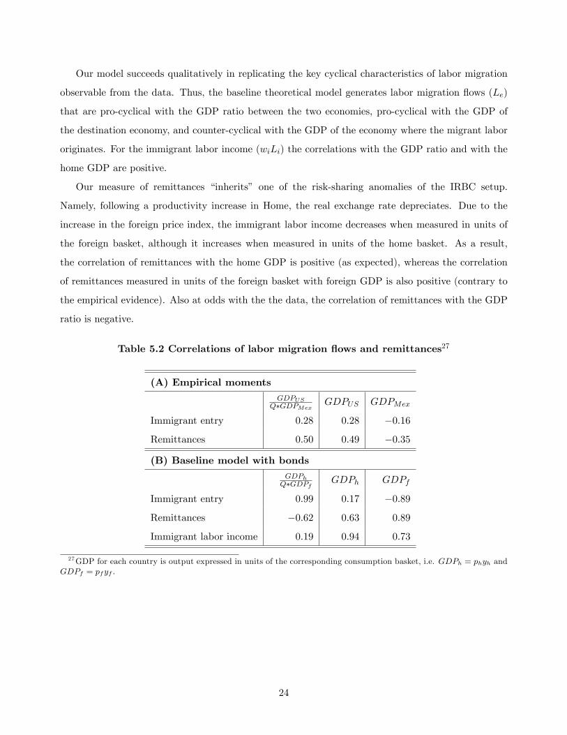
Our model succeeds qualitatively in replicating the key cyclical characteristics of labor migration

observable from the data. Thus, the baseline theoretical model generates labor migration �ows (Le)

that are pro-cyclical with the GDP ratio between the two economies, pro-cyclical with the GDP of

the destination economy, and counter-cyclical with the GDP of the economy where the migrant labor

originates. For the immigrant labor income (wiLi) the correlations with the GDP ratio and with the

home GDP are positive.

Our measure of remittances �inherits� one of the risk-sharing anomalies of the IRBC setup.

Namely, following a productivity increase in Home, the real exchange rate depreciates. Due to the

increase in the foreign price index, the immigrant labor income decreases when measured in units of

the foreign basket, although it increases when measured in units of the home basket. As a result,

the correlation of remittances with the home GDP is positive (as expected), whereas the correlation

of remittances measured in units of the foreign basket with foreign GDP is also positive (contrary to

the empirical evidence). Also at odds with the the data, the correlation of remittances with the GDP

ratio is negative.

Table 5.2 Correlations of labor migration �ows and remittances27

(A) Empirical momentsGDPUS

Q�GDPMexGDPUS GDPMex

Immigrant entry 0:28 0:28 �0:16

Remittances 0:50 0:49 �0:35

(B) Baseline model with bondsGDPhQ�GDPf GDPh GDPf

Immigrant entry 0:99 0:17 �0:89

Remittances �0:62 0:63 0:89

Immigrant labor income 0:19 0:94 0:73

27GDP for each country is output expressed in units of the corresponding consumption basket, i.e. GDPh = phyh andGDPf = pfyf :

24

6 Welfare Implications

6.1 Tightening the Border

In this section we analyze the welfare e¤ects of a sudden and permanent increase in the sunk immi-

gration cost in the baseline setup (from fe = 4 to fe = 5) that could be related to an increase in

border enforcement. The transition paths to a new steady state in Figure 8 show that the declining

availability of immigrant labor makes capital less productive and therefore dampens investment, which

leads to a decline in the capital stock. Due to the higher entry barriers, �rms initially substitute the

immigrant for native labor. Despite the lack of increase in native wages, the inter-temporal optimiza-

tion determines native households to commit more hours in the present, when wages and the return

on capital (interest rate) are signi�cantly higher, than in the future. However, as the rate of capital

depletion decreases, the incentive for inter-temporal substitution weakens and labor supply increases

again, however without exceeding the original steady state.

While the impulse response analysis previously done illustrated the workings of the model, the

quantitative welfare analysis needs to take into account that permanent changes in border enforcement

have not only cyclical but also permanent e¤ects on the balanced-growth path. We solve the model

using a second-order approximation to the policy function around the steady state and consider both

temporary stochastic, and permanent deterministic shocks which are perfectly anticipated by economic

agents.28 We study the welfare e¤ect of the permanent increase in the sunk cost over a wide range of

values for the elasticity of substitution between immigrant and native labor in the baseline model, i.e.

� 2 [0:5; 2:5].

We de�ne welfare (Vt) as the present discounted value of the stream of expected utility. Thus,

we compare the welfare of home households in the initial steady-state (V0) with their welfare as of

the period t0 when the increase in the sunk cost of immigration takes place. The welfare level as of

the period t0 takes into account the discounted stream of utilities that the representative household

achieves at all periods during the transition path to the new steady state after the permanent increase

in the sunk cost of emigration:

Vt0 = Et01Xv=t0

�vU�Cv; Lv

�: (62)

Next we de�ne the constants C0 and C1 to denote the permanent streams of aggregate consumption

that would generate the welfare values V0 and Vt0 : V0 = 11�� ln(C0); Vt0 =

11�� ln(C1); and compute

28We add the future values of the deterministic balanced growth path to the list of state variables (see Juillard, 2006,for details).

25

the consumption-equivalent welfare gain (� > 0) or loss (� < 0) that corresponds to the permanent

increase of the barriers to immigration:� =�C1C0� 1

��100: The results in Figure 9 show that the home

economy experiences a consumption-equivalent welfare loss for the entire range of values � 2 [0:5; 2:5]

of the elasticity of substitution between immigrant and native labor. In particular, the loss increases

with the degree of complementarity between capital and immigrant labor.

6.2 Alternative Model: Gradual Increase in the Share of Native Skilled

This section explores the impact of immigration barriers on welfare in the presence of a gradual and

permanent increase in the share of skilled native labor in Home. In the extended model with two types

of native labor (skilled and unskilled), we introduce a deterministic growth path in the share of skilled

native labor in the total population, allowing it to increase from 0.90 to 0.97 over 20 years. In our

model parameterization this number accounts for the share of natives without a high school diploma.

We assume that households take into account with perfect certainty the expected growth path

of the share of skilled labor when solving their inter-temporal optimization problem, and compute

the consumption-equivalent welfare gain (or loss) associated with the increasing share of skilled labor

relative to the initial steady state. To this end, we compare the home welfare in the initial steady

state:

V0 =1

1� ���sU

�cs; ls

�+ (1� �) (1� s)U

�cu; lu

�(63)

with home welfare as of period t0 when households learn about the growth path of the share of skilled

labor:

Vt0 = Et01Xv=t0

�v f�svU (cs;v; ls;v) + (1� �) (1� sv)U (cu;v; lu;v)g : (64)

The results in Figure 10 show that the welfare loss increases with the magnitude of barriers to

immigration and with the degree of complementarity between capital and immigrant labor. Although

the immigrant and native unskilled labor are perfect substitutes, the welfare loss su¤ered by the home

unskilled households is o¤set by the larger accumulation of capital which enhances the productivity of

the home skilled labor in the presence of immigration. In particular, for very low values of � (for which

it is particularly di¢ cult to substitute away from unskilled labor), we obtain the paradoxical result

that the economy becomes worse o¤ as it limits the in�ow of immigrants, despite the accumulation of

human capital.

Using the extended model with two types of native labor (skilled and unskilled), we repeat the

welfare analysis with the share of skilled native labor increasing deterministically from a lower initial

26

level (i.e. from 0.60 to 0.67 over 20 years). As shown in Figure 11, in contrast to the previous exercise,

we �nd that the welfare gain increases with border enforcement. When a larger fraction of the native

labor becomes exposed to competition from the immigrant labor, the welfare loss of the home unskilled

o¤sets the welfare gains of the home skilled labor that bene�ts from the greater accumulation of capital.

This leads to an overall welfare loss for the home economy.

To sum up, the results indicate that stricter border enforcement reduces welfare for economies in

which unskilled labor is becoming relatively scarce, particularly when it is hard to substitute unskilled

for skilled labor. In contrast, economies with relatively abundant amounts of unskilled labor experience

welfare losses from lowering the barriers to immigration, particularly when it is easy to substitute

unskilled for skilled labor.

7 Conclusion

This paper attempts to bridge the gap between modern international macroeconomics and immigration

theory. In contrast to the former, we allow for labor mobility across countries; in contrast to the latter,

we consider the business cycle dynamics and account for the transmission of aggregate stochastic

shocks across countries in the presence of labor migration. In this context, we consider the insurance

role of workers� remittances as a substitute for contingent claims in smoothing consumption across

households�members residing in di¤erent countries over the business cycle.

In the baseline model, we introduce labor migration �ows within a parsimonious standard two-

country model of international real business cycles. The incentive to emigrate depends on the di¤erence

between the expected future earnings at the destination and in the country of origin, as well as on

the perceived sunk costs of labor migration which re�ects the immigration policy at the destination.

Immigration stimulates the accumulation of capital in the destination economy, which in turn increases

the productivity of native labor. The baseline model successfully matches the cyclical dynamics of labor

migration which we document using U.S. and Mexican data on border apprehensions. International

borrowing and lending facilitate capital �ows and reduce the incentive of foreign labor to emigrate in

steady state. Over the business cycle, however, the �ow of capital towards the expanding economy

reinforces the cyclical pattern of labor migration.

In an alternative speci�cation, we extend the baseline model to allow for skill heterogeneity among

home households in the presence of capital-skill complementarity. The overall welfare gain from un-

skilled immigration for the destination economy increases with the degree of complementarity between

27

the skilled and unskilled labor, as well as with the share of the skilled in total native labor. At the

sectoral level, the in�ow of unskilled immigrants harms the welfare of unskilled native workers, but

a compensation policy mechanism in the form of a countercyclical tax on the immigrant wage can

potentially address this issue.

International real business cycle models have di¢ culty in reconciling their risk sharing implications

with the empirical evidence. Recent contributions properly address these concerns while extending

the standard setup (see for example, Boz et al, 2008 Corsetti et al, 2008, Rabanal et al, 2008, among

others). Accounting for these contributions can improve the match between our model�s implications

and the data. Finally, although we acknowledge the importance of the cross-country migration of

skilled labor, we do not model it in this paper. Future research should explore these issues.

References

[1] Acosta, P. (2006), "Occupational Choice, Migration and Remittances in El Salvador," mimeo.

[2] Acosta, P., E. Lartey, and F. Mandelman (2007), "Remittances and the Dutch disease," Federal

Reserve Bank of Atlanta Working Paper 2007-08.

[3] Aguiar, M. and G. Gopinath (2007), "Emerging Market Business Cycles: The Cycle is the Trend,"

Journal of Political, 115(1): 69-102.

[4] Amuedo-Dorantes, C., and S. Pozo (2004), "Workers�Remittances and the Real Exchange Rate:

A Paradox of Gifts," World Development 32(8): 1407-1417.

[5] Attanasio, O., and S. Davis. (1996), "Relative Wage movements and the Distribution of Con-

sumption,"Journal of Political Economy, 104(6): 1227-1262.

[6] Backus, D. K., P.J. Kehoe, and F.E. Kydland, (1994), "Dynamics of the Trade Balance and the

Terms of Trade: The J-Curve?" American Economic Review, 84(1): 84-103.

[7] Backus, D. K., P.J. Kehoe, and F.E. Kydland, (1992), "International Real Business Cycles,"

Journal of Political Economy 100(4): 754-775.

[8] Backus, D. K., and G.W. Smith (1993), "Consumption and Real Exchange Rates in Dynamic

Economies with Non-traded Goods," Journal of International Economics 35: 297-316.

[9] Banco de México (2004), Informe Anual 2004.

28

[10] Bilbie, F.O., F. Ghironi, and M.J. Melitz (2006), "Endogenous Entry, Product Variety, and

Business Cycles," mimeo, Boston College.

[11] Bodenstein, M. (2008), "Trade Elasticity of Substitution and Equilibrium Dynamics," IFDP 934,

Federal Reserve Board.

[12] Borjas, G. J. (1995), "The Economic Bene�ts from Immigration," Journal Economic Perspectives

9(2): 3-22.

[13] Borjas, G.J., J. Grogger, and G.H. Hanson (2008), "Imperfect Substitution Between Immigrants

and Natives: A Reappraisal," NBER Working Paper 13887.

[14] Boz, E., B. Durdu, and C. Daude (2008), "Emerging Market Business Cycles Revisited: Learning

about the Trend," IFDP 927, Federal Reserve Board.

[15] Chami, R., T. Cosimano, and M. Gapen (2006), "Beware of Emigrants Bearing Gifts: Optimal

Fiscal and Monetary Policy in the Presence of Remitttances," IMF Working Paper 06/61.

[16] Corsetti, G., L. Dedola, and S. Leduc (2008), "International Risk Sharing and the Transmission

of Productivity Shocks," Review of Economic Studies, 75(2): 443-473.

[17] Djacic (1987), "Illegal Alliens, Unemployment, and Immigration Policy," Journal of Development

Economics, 12(1):99-116.

[18] Durdu, C.B., and S. Sayan (2008), "Emerging Market Business Cycles with Remittance Fluctu-

ations", IMF Sta¤ Papers, forthcoming.

[19] Esteves, R., and D. Khoudour-Castéras (2008), " A Fantastic Rain of Gold: European Migrants�

Remittances and the Balance of Payments Adjustment during the Gold Standard Period," mimeo,

Simon Fraser University.

[20] Ghironi F. and M.J. Melitz (2005), "International Trade and Macroeconomic Dynamics with

Heterogeneous Firms," The Quarterly Journal of Economics, 120(3): 865-915.

[21] Gordon, I., T. Travers and C. Whitehead (2007), "The Impact of Recent Immigration on the

London Economy," mimeo, London School of Economics and Political Science.

[22] Grogger, J., and G. H. Hanson (2008), "Income Maximization and the Selection and Sorting of

International Migrants," NBER Working Paper 13821.

29

[23] Hamilton, B., and J. Whalley (1984), "E¢ ciency and Distributional Implications of Global Re-

strictions on Labour Mobility: Calculations and Policy Implications," Journal of Development

Economics, 14(1): 61-75.

[24] Hanson, G., and C. McIntosh (2007), "The Great Mexican Emigration," NBER Working Paper

13675.

[25] Hanson, G., and A. Spilimbergo (1999), "Illegal Immigration, Border Enforcement, and Relative

Wages: Evidence from Apprehensions at the U.S.-Mexico Border," American Economic Review,

89(5): 1337-1357.

[26] Hanson, G. (2005), "Emigration, Remittances and Labor Force Participation in Mexico," mimeo,

University California-San Diego.

[27] Hanson, G. (2006), "Illegal Immigration from Mexico to the United States," NBER Working

Paper 12141.

[28] Heathcote, J., and F. Perri (2002), "Financial Autarky and International Business Cycles," Jour-

nal of Monetary Economics 49: 601-627.

[29] Hernández-Coss, R. (2005), "The U.S.�Mexico Remittance Corridor: Lessons on Shifting from

Informal to Formal Transfer Systems," World Bank Working Paper 47.

[30] Hotchkiss, J. L., and M. Quispe-Agnoli (2008), "The Labor Market Experience and Impact of

Undocumented Workers," Federal Reserve Bank of Atlanta Working Paper 2008-7c,

[31] Jerome, H. (1926), Migration and Business Cycles. New York, National Bureau of Economic

Research.

[32] Juillard, M. (2006), "Policy change and DSGE models," mimeo, CEPREMAP and University of

Paris 8.

[33] King, R., C. Plosser, and S. Rebelo (1988), "Production, Growth and Business Cycles : I. The

Basic Neoclassical Model," Journal of Monetary Economics 21(2-3): 195-232.

[34] Klein, P. and Ventura, G. (2007). "Productivity Di¤erences and the Dynamic E¤ects of Labor

Movements,"mimeo, Uiversity of Iowa.

30

[35] Krueger, D., and F. Perri (2007), "How Does Household Consumption Respond to Income Shocks?

Evidence from Italy and Theoretical Explanations," mimeo, University of Pennsylvania.

[36] Krusell, P.; Ohanian, L., J. V. Rios-Rull, and G. L. Violante (2000), "Capital-Skill Complemen-

tarity and Inequality: A Macroeconomic Analysis," Econometrica, 68(5): 1029-1054.

[37] Lartey, E., F. Mandelman, and P. Acosta (2008), "Remittances, Exchange Rate Regimes, and

the Dutch Disease: A Panel Data Analysis," Federal Reserve Bank of Atlanta WP 2008-12.

[38] Lindquist, M. (2004), "Capital-Skill Complementarity and Inequality Over the Business Cycle,"

Review of Economic Dynamics, 7(3):519-540.

[39] López, H., M. Bussolo, and L. Molina (2007), "Remittances and the Real Exchange Rate", World

Bank Policy Research Working Paper 4213.

[40] Lucas, R (1990). "Why Doesn�t Capital Flow from Rich to Poor Countries," American Economic

Review 80 (2): 92�96.

[41] Moses, J.W., and B.Letnes (2004), "The Economic Costs to International Labor Restrictions:

Revisiting the Empirical Discussion," World Development, 32(10): 1609-1626.

[42] O�Rourke, K.H.; J.G. Williamson (1999), "The Heckscher-Ohlin Model Between 1400 and 2000:

When It Explained Factor Price Convergence, When It Did Not, and Why," NBER Working

Paper 7411.

[43] Polgreen, L., and P. Silos (2005), "Capital-Skill Complementarity and Inequality: a Sensitivity

Analysis," Federal Reserve Bank of Atlanta Working Paper 2005-20.

[44] Rabanal, P., J.F. Rubio-Ramírez (2008), and V. Tuesta"Cointegrated TFP Processes and Inter-

national Business Cycles," mimeo, Duke University.

[45] Ratha, D., and Z. Xu (2008), Migration and Remittances Factbook, World Bank.

[46] Reserve Bank of Australia (2007), Immigration and Labor Supply, Reserve Bank Bulletin, Sep-

tember.

[47] Reyes, B. (1997), "Dynamics of Integration: Return Migration to Western Mexico," Public Policy

Institute of California, in Research Brief, Issue 4.

31

[48] Rodriguez-Zamora, C. (2008), "An Unintended Consequence of Border Enforcement," mimeo,

University of Texas at Austin.

[49] Sjaastad, L. (1962), "The Costs and Returns of Human Migration," Journal of Political Economy,

70(5): 80-93.

[50] Sweetman, A. (2004), "Immigrant Source Country Educational Quality and Canadian Labour

Market Outcomes," Analytical Studies Branch Research Paper Series 2004234e, Statistics Canada,

Analytical Studies Branch.

[51] U.S. Census Bureau (2007), Current Population Survey. Annual Social and Economic Supplement.

[52] Urrutia, C. (1998), "On the Self-Selection of Immigrants," mimeo, Universidad Carlos III de

Madrid.

[53] Walmsley, T., Winters, L. (2003), "Relaxing the Restrictions on the Temporary Movements of

Natural Persons: A Simulation Analysis," CEPR Discussion Papers 3719.

32

A Appendix

A.1 Baseline Model of Labor Migration with Financial Autarky, Steady State

The foreign economy In steady state, A� = 1. With the classic Cobb-Douglas production

function Yf = (K�)���L�f

�1���, it is straightforward to solve for the steady state in the foreign

economy:

r� =1� ����

; (65)

YfK� =

r� + ��

��; (66)

K� =

�YfK�

� 1���1

L�f ; (67)

Yf =

�YfK�

�K� =

�r� + ��

��

� �����1

L�f ; (68)

w� = (1� ��) YfL�f

= (1� ��)�r� + ��

��

� �����1

; (69)

I� = ��K�: (70)

The home economy For the home economy, we solve the steady state numerically using a

system of eight non-linear equations (71, 72, 76-81) in eight unknowns (Yh, K, Li, Yh2, Yf1, ph, pf ,

Q), as described below.

Equations 1-2: With A = 1, output and the marginal product of capital are:

Yh = K�h 1� (Li)

��1� + (1� )

1� (�Ln)

��1�

i ���1 (1��)

; (71)

@Yh@K

= �YhK= r + �: (72)

Equation 3: Using the steady-state expression for the present discounted value of the future gains

from immigration, feQ�1wi =��(1��l)1���(1��l)d, we obtain:

Q�1wi = w� + d; (73)

= w� +1� ��(1� �l)��(1� �l)

feQ�1wi: (74)

Thus, the steady state ratio of the immigrant wage and the wage in in the country of origin expressed

33

in units of the same consumption basket is:

� � wiw�Q

=

�1� 1� �

�(1� �l)��(1� �l)

fe

��1; (75)

where � = 1 when fe = 0, i.e. with zero sunk cost of labor migration, the wage ratio is equal to unit.

Next, we insert wi =@Yh@Li

and w� = @Yf@L� into the previous equation to obtain:

(1� �) (Yh)1����(1��) K

�(��1)�(1��)

�

Li;t

� 1�

| {z }wi

= �(1� ��)�r� + ��

��

� �����1

| {z }w�

Q: (76)

Equation 4: The balanced current account condition implies:

phYh2 = pfQYf1 + Liwi �LiL�C�Q; (77)

where wi is given above, and:

Y � =h!� 1� (Yf � Yf1)

��1� + (1� !�)

1� (Yh1)

��1�

i ���1

;

Yf =

�r� + ��

��

� �����1

(L� � Li) ;

Le =�l

1� �lLi:

Equations 5-6: We write the demand ratios for the two intermediate goods in each economy as:

Yh � Yh2Yf1

=!

1� !

�phpfQ

���; (78)

Yf � Yf1Yh2

=!�

1� !�

�pfQ

ph

����: (79)

Equations 7-8: The price indexes for the composite good of each country are:

1 = ! (ph)1�� + (1� !)(pfQ)1��; (80)

1 = !� (pf )1��� + (1� !�)

�phQ

�1���: (81)

34

A.2 Alternative Model of Labor Migration with Financial Autarky, Steady State

The presence of skill heterogeneity among native labor (skilled and unskilled) in Home requires several

modi�cations in the calculation of steady state relative to the baseline model. In the system of eight

equations in eight unknowns described above, Ln becomes Ls (i.e. native skilled labor). One must

also distinguish between individual vs. aggregate labor supply (i.e. lj vs. Lj) and consumption (i.e.

cj vs. Cj) for the representative skilled and unskilled households (where j 2 fs; ug). Thus, equations

71, 76 and 77 are replaced by:

(Yh)��1� =

1� (Li + Lu)

��1� + (1� )

1�

h�1�K

��1� + (1� �)

1� (�Ls)

��1�

i ���1

��1�; (82)�

Yh

Li + Lu

� 1�

| {z }wi

= �(1� ��)�r� + ��

��

� �����1

| {z }w�

Q; (83)

phYh2 = pfQYf1 + Li

�

YhLi + Lu

� 1�

| {z }wi

� LiL�C�Q: (84)

A.3 BaselineModel of LaborMigration with International Trade in Bonds, Steady

State

The presence of quadratic costs of adjustment for bond holdings allows us to pin down their steady-

state levels. From 1 + �Bh = �(1 + rb), 1 + �B�h = ��(1 + rb) and Bh +B�h = 0; it follows that:

rb =2

� + ��� 1; (85)

Bh = �B�h =�(1 + rb)� 1

�: (86)

Similarly, using that 1+�Bf = �(1+ rb�), 1+�B�f = ��(1+ rb�) and Bf +B�f = 0; it follows that:

rb� =2

� + ��� 1 = rb; (87)

Bf = �B�f =�(1 + rb�)� 1

�: (88)

Finally, the balanced current account condition (77) is replaced by the expression for the balance

35

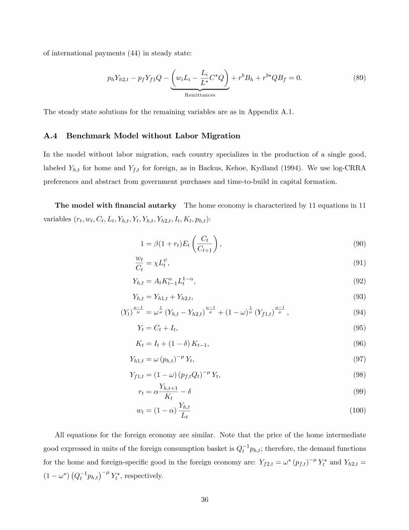
of international payments (44) in steady state:

phYh2;t � pfYf1Q��wiLi �

LiL�C�Q

�| {z }

Remittances

+ rbBh + rb�QBf = 0: (89)

The steady state solutions for the remaining variables are as in Appendix A.1.

A.4 Benchmark Model without Labor Migration

In the model without labor migration, each country specializes in the production of a single good,

labeled Yh;t for home and Yf;t for foreign, as in Backus, Kehoe, Kydland (1994). We use log-CRRA

preferences and abstract from government purchases and time-to-build in capital formation.

The model with �nancial autarky The home economy is characterized by 11 equations in 11

variables (rt; wt; Ct; Lt; Yh;t; Yt; Yh;t; Yh2;t; It;Kt; ph;t):

1 = �(1 + rt)Et

�CtCt+1

�; (90)

wtCt= �L t ; (91)

Yh;t = AtK�t�1L

1��t ; (92)

Yh;t = Yh1;t + Yh2;t; (93)

(Yt)��1� = !

1� (Yh;t � Yh2;t)

��1� + (1� !)

1� (Yf1;t)

��1� ; (94)

Yt = Ct + It; (95)

Kt = It + (1� �)Kt�1; (96)

Yh1;t = ! (ph;t)�� Yt; (97)

Yf1;t = (1� !) (pf;tQt)�� Yt; (98)

rt = �Yh;t+1Kt

� � (99)

wt = (1� �)Yh;tLt

(100)

All equations for the foreign economy are similar. Note that the price of the home intermediate

good expressed in units of the foreign consumption basket is Q�1t ph;t; therefore, the demand functions

for the home and foreign-speci�c good in the foreign economy are: Yf2;t = !� (pf;t)�� Y �t and Yh2;t =

(1� !�)�Q�1t ph;t

���Y �t , respectively.

36

Technology follows the process:

logAt = � logAt�1 + et;

logA�t = � logA�t�1 + e�t

The real exchange rate Qt is pinned down by the trade balance, measured in units of the home

composite good:

NXt = Yh2;tph;t| {z }exports

� Yf1;tpf;tQt| {z }imports

: (101)

Under �nancial autarky and without remittances, NXt = 0.

Financial integration, trade in risk-free bonds International trade in risk-free bonds (with

quadratic cost of adjustment of bond holdings) adds 6 extra variables (i.e. the rates of return of the

home and foreign bonds, rbt and rb�t ; holdings of the home and foreign bonds by home households, Bh;t

and Bf;t; holdings of the home and foreign bonds by foreign households, B�h;t and B�f;t) and 6 new

equations to the model with �nancial autarky:

1 + �Bh;t+1 = �Et

�(1 + rbt+1)

CtCt+1

�; (102)

1 + �Bf;t+1 = �Et

�Qt+1Qt

(1 + rb�t+1)CtCt+1

�; (103)

1 + �B�h;t+1 = ��Et

�QtQt+1

(1 + rbt+1)C�tC�t+1

�; (104)

1 + �B�f;t+1 = ��Et

�(1 + rb�t+1)

C�tC�t+1

�; (105)

Bh;t+1 +B�h;t+1 = 0; (106)

Bf;t+1 +B�f;t+1 = 0: (107)

The expression for the balance of international payments replaces the balanced trade condition from

the model with �nancial autarky:

ph;tYh2;t � pf;tQtYf1;t + rbtBh;t + rb�t QtBf;t = 0: (108)

37

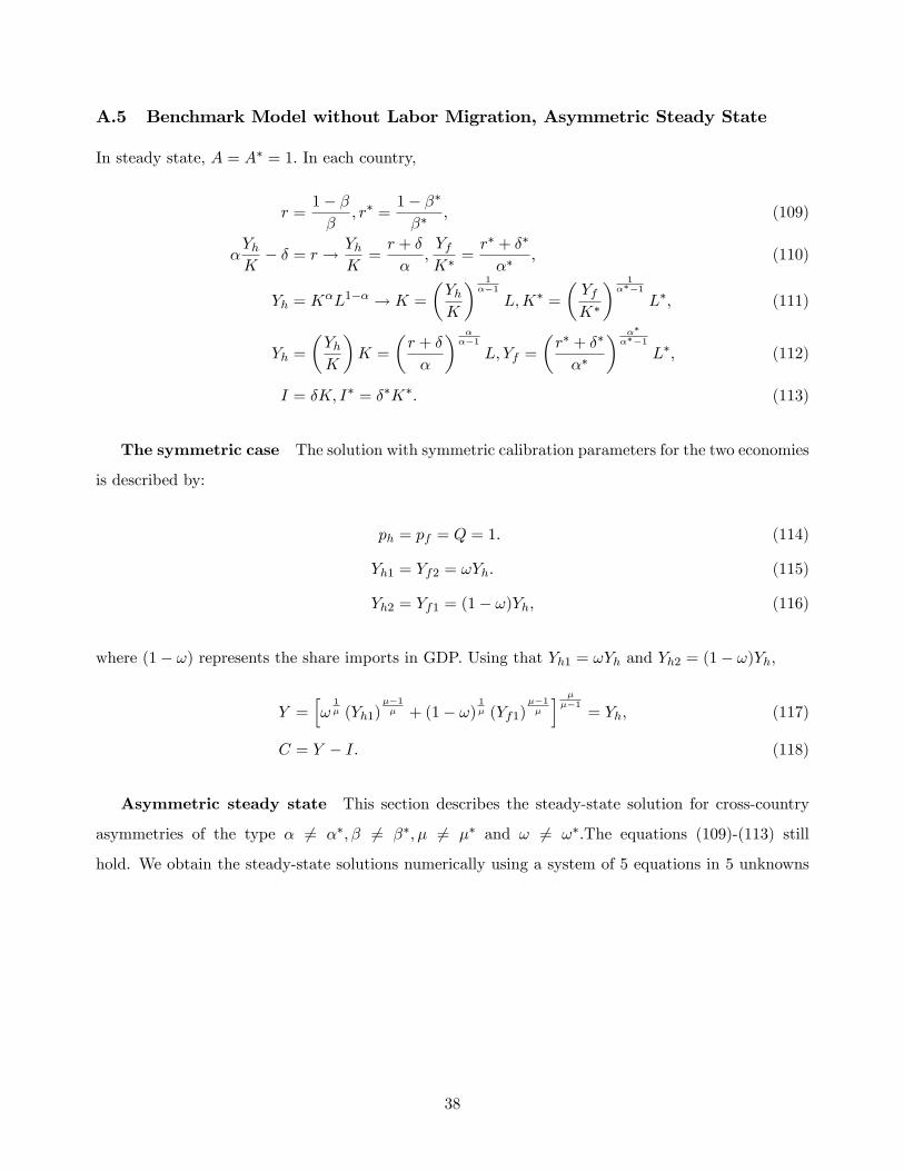
A.5 Benchmark Model without Labor Migration, Asymmetric Steady State

In steady state, A = A� = 1: In each country,

r =1� ��

; r� =1� ����

; (109)

�YhK� � = r ! Yh

K=r + �

�;YfK� =

r� + ��

��; (110)

Yh = K�L1�� ! K =

�YhK

� 1��1

L;K� =

�YfK�

� 1���1

L�; (111)

Yh =

�YhK

�K =

�r + �

�

� ���1

L; Yf =

�r� + ��

��

� �����1

L�; (112)

I = �K; I� = ��K�: (113)

The symmetric case The solution with symmetric calibration parameters for the two economies

is described by:

ph = pf = Q = 1: (114)

Yh1 = Yf2 = !Yh: (115)

Yh2 = Yf1 = (1� !)Yh; (116)

where (1� !) represents the share imports in GDP. Using that Yh1 = !Yh and Yh2 = (1� !)Yh,

Y =h!1� (Yh1)

��1� + (1� !)

1� (Yf1)

��1�

i ���1

= Yh; (117)

C = Y � I: (118)

Asymmetric steady state This section describes the steady-state solution for cross-country

asymmetries of the type � 6= ��; � 6= ��; � 6= �� and ! 6= !�:The equations (109)-(113) still

hold. We obtain the steady-state solutions numerically using a system of 5 equations in 5 unknowns

38

(Yh1; Yf2; ph; pf ; Q):

Yh1Yf � Yf2

=!

1� !

�phpfQ

���; (119)

Yf2Yh � Yh2

=!�

1� !�

�pfQ

ph

����; (120)

1 = ! (ph)1�� + (1� !)(pfQ)1��; (121)

1 = !� (pf )1��� + (1� !�)

�phQ

�1���(122)

In �nancial autarky, the balanced trade condition is:

Yh2ph � Yf1pfQ = 0: (123)

With �nancial integration, balanced trade is replaced by the expression for the balance of interna-

tional payments:

phYh2 � pfQYf1 + rbBh + rb�QBf = 0: (124)

39

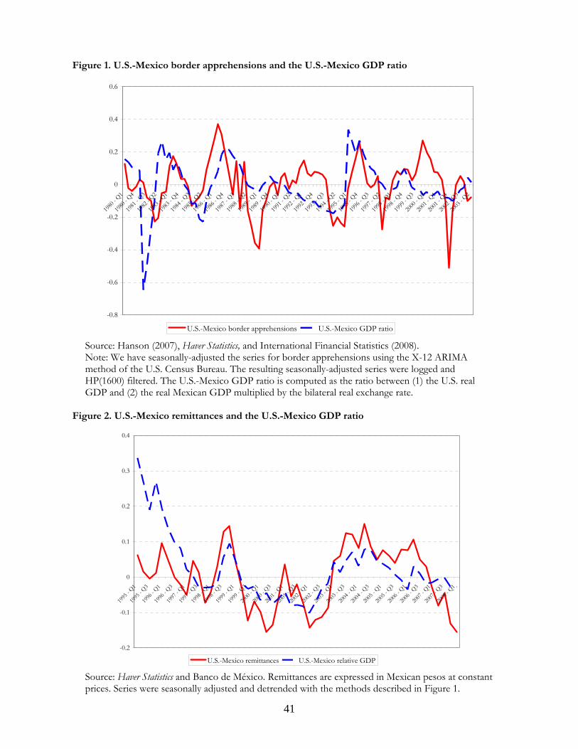
41

Figure 1. U.S.-Mexico border apprehensions and the U.S.-Mexico GDP ratio

-0.8

-0.6

-0.4

-0.2

0

0.2

0.4

0.6

1980

- Q1

1980

- Q4

1981

- Q3

1982

- Q2

1983

- Q1

1983

- Q4

1984

- Q3

1985

- Q2

1986

- Q1

1986

- Q4

1987

- Q3

1988

- Q2

1989

- Q1

1989

- Q4

1990

- Q3

1991

- Q2

1992

- Q1

1992

- Q4

1993

- Q3

1994

- Q2

1995

- Q1

1995

- Q4

1996

- Q3

1997

- Q2

1998

- Q1

1998

- Q4

1999

- Q3

2000

- Q2

2001

- Q1

2001

- Q4

2002

- Q3

2003

- Q2

U.S.-Mexico border apprehensions U.S.-Mexico GDP ratio

Source: Hanson (2007), Haver Statistics, and International Financial Statistics (2008). Note: We have seasonally-adjusted the series for border apprehensions using the X-12 ARIMA method of the U.S. Census Bureau. The resulting seasonally-adjusted series were logged and HP(1600) filtered. The U.S.-Mexico GDP ratio is computed as the ratio between (1) the U.S. real GDP and (2) the real Mexican GDP multiplied by the bilateral real exchange rate.

Figure 2. U.S.-Mexico remittances and the U.S.-Mexico GDP ratio

-0.2

-0.1

0

0.1

0.2

0.3

0.4

1995

- Q1

1995

- Q3

1996

- Q1

1996

- Q3

1997

- Q1

1997

- Q3

1998

- Q1

1998

- Q3

1999

- Q1

1999

- Q3

2000

- Q1

2000

- Q3

2001

- Q1

2001

- Q3

2002

- Q1

2002

- Q3

2003

- Q1

2003

- Q3

2004

- Q1

2004

- Q3

2005

- Q1

2005

- Q3

2006

- Q1

2006

- Q3

2007

- Q1

2007

- Q3

2008

- Q1

U.S.-Mexico remittances U.S.-Mexico relative GDP

Source: Haver Statistics and Banco de México. Remittances are expressed in Mexican pesos at constant prices. Series were seasonally adjusted and detrended with the methods described in Figure 1.

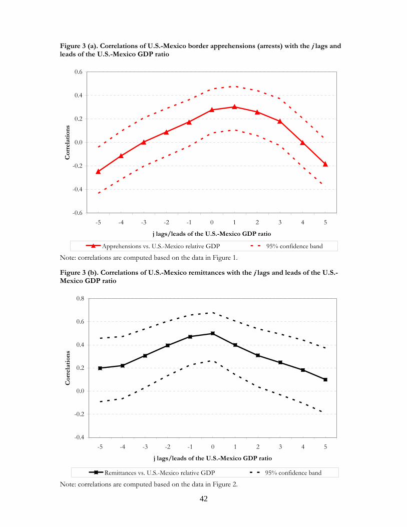
42

Figure 3 (a). Correlations of U.S.-Mexico border apprehensions (arrests) with the j lags and leads of the U.S.-Mexico GDP ratio

-0.6

-0.4

-0.2

0.0

0.2

0.4

0.6

-5 -4 -3 -2 -1 0 1 2 3 4 5

j lags/leads of the U.S.-Mexico GDP ratio

Cor

rela

tion

s

Apprehensions vs. U.S.-Mexico relative GDP 95% confidence band Note: correlations are computed based on the data in Figure 1. Figure 3 (b). Correlations of U.S.-Mexico remittances with the j lags and leads of the U.S.-Mexico GDP ratio

-0.4

-0.2

0.0

0.2

0.4

0.6

0.8

-5 -4 -3 -2 -1 0 1 2 3 4 5

j lags/leads of the U.S.-Mexico GDP ratio

Cor

rela

tion

s

Remittances vs. U.S.-Mexico relative GDP 95% confidence band

Note: correlations are computed based on the data in Figure 2.

43

Figure 4. Baseline model with financial autarky

Each panel shows the response (percent deviations from steady state) to a transitory 1 percent increase in home productivity, for the cases with high sunk cost (fe =6, dashed) and low sunk cost (fe =1, solid).

44

Figure 5. Baseline model with financial autarky, low elasticity of substitution between native and immigrant labor

Each panel shows the response (percent deviations from steady state) to a transitory 1 percent increase in home productivity, under high complementarity between the native and immigrant labor (θ = 0.5), for the cases with high sunk cost (fe =6, dashed) and low sunk cost (fe =1, solid).

45

Figure 6. Baseline model with financial integration

Each panel shows the response (percent deviations from steady state) to a transitory 1 percent increase in home productivity, for the cases with high sunk cost (fe =6, dashed) and low sunk cost (fe =1, solid). The model allows for international trade in risk-free bonds (with adjustment cost parameter π = 0.005).

46

Figure 7. Alternative model with financial autarky

Each panel shows the response (percent deviations from steady state) to a transitory 1 percent decrease in home productivity in the alternative model (i.e. in which we allow for skill heterogeneity among the native labor, and we assume capital-skill complementarity), in the presence of (1) counter-cyclical immigration tax (solid), and (b) sunk emigration cost (dashed).

47

Figure 8. Baseline model with financial autarky: permanent increase in border enforcement

Each panel shows the transition path of the model’s variables with a permanent increase in the sunk emigration cost (sudden increase from fe =4 to fe =5). Figure 9. Welfare analysis, baseline model with financial autarky

Consumption-equivalent welfare gain/loss with a permanent increase in the sunk emigration cost (sudden increase from fe =4 to fe =5).

48

Figure 10. Welfare analysis, alternative model with financial autarky: implications of a rising share of skilled labor (1)

Consumption-equivalent welfare gain/loss from a rising share of native skilled labor (from 0.9 to 0.97 over 20 years), in the presence of the sunk emigration cost. Figure 11. Welfare analysis, alternative model with financial autarky: implications of a rising share of skilled labor (2)

Consumption-equivalent welfare gain/from a rising share of native skilled labor (from 0.6 to 0.67 over 20 years), in the presence of the sunk emigration cost.