atlas_v2
TRANSCRIPT

SILVACO International4701 Patrick Henry Drive, Bldg. 1 February 2000Santa Clara, CA 95054 Telephone (408) 567-1000FAX: (408) 496-6080
ATLAS User’s Manual DEVICE SIMULATION SOFTWARE
Volume II

ATLAS User’s Manual
Copyright 2000SILVACO International4701 Patrick Henry Drive, Building 1Santa Clara, CA 95054
Phone: (408) 567-1000FAX: (408) 496-6080
Notice
The information contained in this document is subject to change without notice.
SILVACO International MAKES NO WARRANTY OF ANY KIND WITH REGARD TO THISMATERIAL, INCLUDING, BUT NOT LIMITED TO, THE IMPLIED WARRANTY OF FITNESSFOR A PARTICULAR PURPOSE.
SILVACO International Inc. shall not be liable for errors contained herein or for incidental or consequentialdamages in connection with the furnishing, performance, or use of this material.
This document contains proprietary information, which is protected by copyright. All rights are reserved. Nopart of this document may be photocopied, reproduced, or translated into another language without the priorwritten consent of SILVACO International.
Simulation Standard, TCADDrivenCAD, Virtual Wafer Fab, Analog Alliance, Legacy, ATHENA, ATLAS,FASTATLAS, ODIN, VYPER, CRUSADE, RESILIENCE, DISCOVERY, CELEBRITY, Production Tools,Automation Tools, Interactive Tools, TonyPlot, DeckBuild, DevEdit, Interpreter, ATHENA Interpreter,ATLAS Interpreter, Circuit Optimizer, MaskViews, PSTATS, SSuprem3, SSuprem4, Elite, Optolith,Flash, Silicides, SPDB, CMP, MC Deposit, MC Implant, Process Adaptive Meshing, S-Pisces, Blaze,Device3D, Thermal3D, Interconnect3D, Blaze 3D, Giga3D, MixedMode3D, TFT, Luminous, Giga,MixedMode, ESD, Laser, FastBlaze, FastMixedMode, FastGiga, FastNoise, MOCASIM, UTMOST,UTMOST II, UTMOST III, UTMOST IV, PROMOST, SPAYN, SmartSpice, MixSim, Twister, FastSpice,SmartLib, SDDL, EXACT, CLEVER, STELLAR, HIPEX, Scholar, SIREN, Escort, Starlet, Expert,Savage, Scout, Guardian, and Envoy – are trademarks of SILVACO International.
© 1990, 1991, 1992, 1993, 1994, 1995, 1996, 1997, 1998, 2000 by SILVACO International Inc.
SILVACO International iii

Reader Comment Sheet
We welcome your evaluation of this manual. Your comments and suggestions help us to improve ourpublications. If you have any responses to the questions below, please let us know. Write your observations,complaints, bug reports, suggestions or comments below.
• Is this manual technically accurate?
• Are the concepts and wording easy to understand?
• Is the size of this manual convenient for you?
• Is the manual's arrangement convenient for you?
• Do you consider this manual to be easily readable?
• Please add any additional relevant comments.
Please fax your comments to SILVACO International, Attention Technical Publications at (408) 496-6080.
iv SILVACO International

Introduction
Intended Audience
The information presented is based on the assumptions that the reader is (1) familiar with the basic terminologyof semiconductor processing and semiconductor device operation, and (2) understands basic operation of thecomputer hardware and operation system being employed.
Introduction
ATLAS is a modular and extensible framework for one, two and three dimensional semiconductor devicesimulation. It is implemented using modern software engineering practices that promote reliability,maintainability, and extensibility. Products that use the ATLAS Framework meet the device simulation needsof all semiconductor application areas.
SILVACO International makes no warranty of any kind with regard to this material, including, but not limitedto, the implied warranty of fitness for a particular purpose.
SILVACO International shall not be liable for errors contained herein or for incidental or consequentialdamages in connection with furnishing, performance, or use of this material. This document containsproprietary information protected by copyright. All rights are reserved. No part of this document may bephotocopied, reproduced, or translated into another language without the prior written consent of SILVACOInternational.
Editions are recorded below under History, and are individually listed as Edition 1 through 6. The basic issueof the manual is Edition 1. The date is also noted. A completely revised manual results in a new edition.
History• Edition 1 - July 1, 1993
• Edition 2 - March 1, 1994
• Edition 3 - June 1, 1994
• Edition 4 - October 30, 1996
• Edition 5 - April 30, 1997
• Edition 6 - November 1998
• Edition 7 - February 2000
SILVACO International v

ATLAS User’s Manual
This page intentionally left blank.
vi SILVACO International

Table of Contents
Chapter 11:3D Device Simulation . . . . . . . . . . . . . . . . . . . . . . . . . . . . . . . . . . . . . . . . . . . . . . . . . . . . . 11-1
Overview of 3D Device Simulation Programs . . . . . . . . . . . . . . . . . . . . . . . . . . . . . . . . . . . . . . . . . . . . . . . . . . . 11-1Device3D . . . . . . . . . . . . . . . . . . . . . . . . . . . . . . . . . . . . . . . . . . . . . . . . . . . . . . . . . . . . . . . . . . . . . . . . . . . . . . 11-1Blaze3D . . . . . . . . . . . . . . . . . . . . . . . . . . . . . . . . . . . . . . . . . . . . . . . . . . . . . . . . . . . . . . . . . . . . . . . . . . . . . . . 11-1Giga3D . . . . . . . . . . . . . . . . . . . . . . . . . . . . . . . . . . . . . . . . . . . . . . . . . . . . . . . . . . . . . . . . . . . . . . . . . . . . . . . 11-1TFT3D . . . . . . . . . . . . . . . . . . . . . . . . . . . . . . . . . . . . . . . . . . . . . . . . . . . . . . . . . . . . . . . . . . . . . . . . . . . . . . . . 11-2MIXEDMODE3D . . . . . . . . . . . . . . . . . . . . . . . . . . . . . . . . . . . . . . . . . . . . . . . . . . . . . . . . . . . . . . . . . . . . . . . . 11-2Quantum3D . . . . . . . . . . . . . . . . . . . . . . . . . . . . . . . . . . . . . . . . . . . . . . . . . . . . . . . . . . . . . . . . . . . . . . . . . . . . 11-2Luminous . . . . . . . . . . . . . . . . . . . . . . . . . . . . . . . . . . . . . . . . . . . . . . . . . . . . . . . . . . . . . . . . . . . . . . . . . . . . . . 11-2
3D Structure Generation . . . . . . . . . . . . . . . . . . . . . . . . . . . . . . . . . . . . . . . . . . . . . . . . . . . . . . . . . . . . . . . . . . . . 11-3ATLAS Syntax For 3D Structure Generation . . . . . . . . . . . . . . . . . . . . . . . . . . . . . . . . . . . . . . . . . . . . . . . 11-3DevEdit3D Interface . . . . . . . . . . . . . . . . . . . . . . . . . . . . . . . . . . . . . . . . . . . . . . . . . . . . . . . . . . . . . . . . . . 11-3
Model And Material Parameter Selection in 3D . . . . . . . . . . . . . . . . . . . . . . . . . . . . . . . . . . . . . . . . . . . . . . . . 11-4Simulation of Single Event Upset . . . . . . . . . . . . . . . . . . . . . . . . . . . . . . . . . . . . . . . . . . . . . . . . . . . . . . . . 11-5User-defined SEU in 3D . . . . . . . . . . . . . . . . . . . . . . . . . . . . . . . . . . . . . . . . . . . . . . . . . . . . . . . . . . . . . . . 11-7
Boundary Conditions in 3D . . . . . . . . . . . . . . . . . . . . . . . . . . . . . . . . . . . . . . . . . . . . . . . . . . . . . . . . . . . . . . . . 11-7External Passive Elements . . . . . . . . . . . . . . . . . . . . . . . . . . . . . . . . . . . . . . . . . . . . . . . . . . . . . . . . . . . . 11-7Thermal Contacts for GIGA3D . . . . . . . . . . . . . . . . . . . . . . . . . . . . . . . . . . . . . . . . . . . . . . . . . . . . . . . . . . 11-7
BLAZE3D Models . . . . . . . . . . . . . . . . . . . . . . . . . . . . . . . . . . . . . . . . . . . . . . . . . . . . . . . . . . . . . . . . . . . . . . . 11-8TFT3D Models . . . . . . . . . . . . . . . . . . . . . . . . . . . . . . . . . . . . . . . . . . . . . . . . . . . . . . . . . . . . . . . . . . . . . . . . . 11-8QUANTUM3D Models . . . . . . . . . . . . . . . . . . . . . . . . . . . . . . . . . . . . . . . . . . . . . . . . . . . . . . . . . . . . . . . . . . . 11-8LUMINOUS3d Models . . . . . . . . . . . . . . . . . . . . . . . . . . . . . . . . . . . . . . . . . . . . . . . . . . . . . . . . . . . . . . . . . . . . 11-8
Numerical Methods for 3D . . . . . . . . . . . . . . . . . . . . . . . . . . . . . . . . . . . . . . . . . . . . . . . . . . . . . . . . . . . . . . . . . . 11-12DC Solutions . . . . . . . . . . . . . . . . . . . . . . . . . . . . . . . . . . . . . . . . . . . . . . . . . . . . . . . . . . . . . . . . . . . . . . . . . . 11-12Transient Solutions . . . . . . . . . . . . . . . . . . . . . . . . . . . . . . . . . . . . . . . . . . . . . . . . . . . . . . . . . . . . . . . . . . . . . 11-12Obtaining Solutions In 3D . . . . . . . . . . . . . . . . . . . . . . . . . . . . . . . . . . . . . . . . . . . . . . . . . . . . . . . . . . . . . . . . 11-12Interpreting the Results From 3D . . . . . . . . . . . . . . . . . . . . . . . . . . . . . . . . . . . . . . . . . . . . . . . . . . . . . . . . . . 11-12More Information . . . . . . . . . . . . . . . . . . . . . . . . . . . . . . . . . . . . . . . . . . . . . . . . . . . . . . . . . . . . . . . . . . . . . . . 11-12
Chapter 12:INTERCONNECT3D . . . . . . . . . . . . . . . . . . . . . . . . . . . . . . . . . . . . . . . . . . . . . . . . . . . . . . . 12-1
Overview . . . . . . . . . . . . . . . . . . . . . . . . . . . . . . . . . . . . . . . . . . . . . . . . . . . . . . . . . . . . . . . . . . . . . . . . . . . . . . . . . 12-1Model Description . . . . . . . . . . . . . . . . . . . . . . . . . . . . . . . . . . . . . . . . . . . . . . . . . . . . . . . . . . . . . . . . . . . . . . . . . 12-1Capacitance and Conductance Calculation . . . . . . . . . . . . . . . . . . . . . . . . . . . . . . . . . . . . . . . . . . . . . . . . . . . . . 12-1
Boundary Conditions . . . . . . . . . . . . . . . . . . . . . . . . . . . . . . . . . . . . . . . . . . . . . . . . . . . . . . . . . . . . . . . . . 12-1
Structure Definition . . . . . . . . . . . . . . . . . . . . . . . . . . . . . . . . . . . . . . . . . . . . . . . . . . . . . . . . . . . . . . . . . . . . . . . . 12-3Tutorial For The MaskViews Interface . . . . . . . . . . . . . . . . . . . . . . . . . . . . . . . . . . . . . . . . . . . . . . . . . . . . . . . . 12-4
Saving Mask Data For INTERCONNECT3D . . . . . . . . . . . . . . . . . . . . . . . . . . . . . . . . . . . . . . . . . . . . . . . 12-4Loading Mask Data Into INTERCONNECT3D . . . . . . . . . . . . . . . . . . . . . . . . . . . . . . . . . . . . . . . . . . . . . . 12-4
Defining Electrodes . . . . . . . . . . . . . . . . . . . . . . . . . . . . . . . . . . . . . . . . . . . . . . . . . . . . . . . . . . . . . . . . . . . . . . 12-4
Model And Material Parameter Selection . . . . . . . . . . . . . . . . . . . . . . . . . . . . . . . . . . . . . . . . . . . . . . . . . . . . . . . 12-6Conductivity Calculations . . . . . . . . . . . . . . . . . . . . . . . . . . . . . . . . . . . . . . . . . . . . . . . . . . . . . . . . . . . . . . . . . 12-6
SILVACO International vii
ATLAS User’s Manual – Volume 2
Capacitance Calculations . . . . . . . . . . . . . . . . . . . . . . . . . . . . . . . . . . . . . . . . . . . . . . . . . . . . . . . . . . . . . . . . . 12-6
Applying CD Variations and Misalignment . . . . . . . . . . . . . . . . . . . . . . . . . . . . . . . . . . . . . . . . . . . . . . . . . . . . . 12-7Numerical Methods . . . . . . . . . . . . . . . . . . . . . . . . . . . . . . . . . . . . . . . . . . . . . . . . . . . . . . . . . . . . . . . . . . . . . . . . 12-7Obtaining Solutions . . . . . . . . . . . . . . . . . . . . . . . . . . . . . . . . . . . . . . . . . . . . . . . . . . . . . . . . . . . . . . . . . . . . . . . . 12-7Interpreting the Results . . . . . . . . . . . . . . . . . . . . . . . . . . . . . . . . . . . . . . . . . . . . . . . . . . . . . . . . . . . . . . . . . . . . 12-7More Information . . . . . . . . . . . . . . . . . . . . . . . . . . . . . . . . . . . . . . . . . . . . . . . . . . . . . . . . . . . . . . . . . . . . . . . . . . 12-7
Chapter 13:THERMAL3D . . . . . . . . . . . . . . . . . . . . . . . . . . . . . . . . . . . . . . . . . . . . . . . . . . . . . . . . . . . . 13-1
Overview . . . . . . . . . . . . . . . . . . . . . . . . . . . . . . . . . . . . . . . . . . . . . . . . . . . . . . . . . . . . . . . . . . . . . . . . . . . . . . . . . 13-13D Structure Generation . . . . . . . . . . . . . . . . . . . . . . . . . . . . . . . . . . . . . . . . . . . . . . . . . . . . . . . . . . . . . . . . . . 13-1
Defining Heat Sources . . . . . . . . . . . . . . . . . . . . . . . . . . . . . . . . . . . . . . . . . . . . . . . . . . . . . . . . . . . . . . . 13-1Defining Heat Sinks . . . . . . . . . . . . . . . . . . . . . . . . . . . . . . . . . . . . . . . . . . . . . . . . . . . . . . . . . . . . . . . . . . 13-1
Model and Material Parameter Selection . . . . . . . . . . . . . . . . . . . . . . . . . . . . . . . . . . . . . . . . . . . . . . . . . . . . . . . 13-2Setting Thermal Conductivity . . . . . . . . . . . . . . . . . . . . . . . . . . . . . . . . . . . . . . . . . . . . . . . . . . . . . . . . . . . . . . 13-2Suggested Parameters For Thermal Conductivity . . . . . . . . . . . . . . . . . . . . . . . . . . . . . . . . . . . . . . . . . . . . . . 13-3
Numerical Methods . . . . . . . . . . . . . . . . . . . . . . . . . . . . . . . . . . . . . . . . . . . . . . . . . . . . . . . . . . . . . . . . . . . . . . . . 13-3Obtaining Solutions In THERMAL3D . . . . . . . . . . . . . . . . . . . . . . . . . . . . . . . . . . . . . . . . . . . . . . . . . . . . . . . . . . 13-3Interpreting The Results From THERMAL3D . . . . . . . . . . . . . . . . . . . . . . . . . . . . . . . . . . . . . . . . . . . . . . . . . . . . 13-4More Information . . . . . . . . . . . . . . . . . . . . . . . . . . . . . . . . . . . . . . . . . . . . . . . . . . . . . . . . . . . . . . . . . . . . . . . . . . 13-4
Chapter 14:Numerical Techniques . . . . . . . . . . . . . . . . . . . . . . . . . . . . . . . . . . . . . . . . . . . . . . . . . . . . . 14-1
Overview . . . . . . . . . . . . . . . . . . . . . . . . . . . . . . . . . . . . . . . . . . . . . . . . . . . . . . . . . . . . . . . . . . . . . . . . . . . . . . . . . 14-1Numerical Solution Procedures . . . . . . . . . . . . . . . . . . . . . . . . . . . . . . . . . . . . . . . . . . . . . . . . . . . . . . . . . . . . 14-1
Meshes . . . . . . . . . . . . . . . . . . . . . . . . . . . . . . . . . . . . . . . . . . . . . . . . . . . . . . . . . . . . . . . . . . . . . . . . . . . . . . . . . . 14-1Mesh Regridding . . . . . . . . . . . . . . . . . . . . . . . . . . . . . . . . . . . . . . . . . . . . . . . . . . . . . . . . . . . . . . . . . . . . . . . 14-2Mesh Smoothing . . . . . . . . . . . . . . . . . . . . . . . . . . . . . . . . . . . . . . . . . . . . . . . . . . . . . . . . . . . . . . . . . . . . . . . . 14-3
Discretization . . . . . . . . . . . . . . . . . . . . . . . . . . . . . . . . . . . . . . . . . . . . . . . . . . . . . . . . . . . . . . . . . . . . . . . . . . . . . 14-3The Discretization Process . . . . . . . . . . . . . . . . . . . . . . . . . . . . . . . . . . . . . . . . . . . . . . . . . . . . . . . . . . . . . . . . 14-3
Non-Linear Iteration . . . . . . . . . . . . . . . . . . . . . . . . . . . . . . . . . . . . . . . . . . . . . . . . . . . . . . . . . . . . . . . . . . . . . . . . 14-4Newton Iteration . . . . . . . . . . . . . . . . . . . . . . . . . . . . . . . . . . . . . . . . . . . . . . . . . . . . . . . . . . . . . . . . . . . . . . . . 14-4Gummel Iteration . . . . . . . . . . . . . . . . . . . . . . . . . . . . . . . . . . . . . . . . . . . . . . . . . . . . . . . . . . . . . . . . . . . . . . . 14-4Block Iteration . . . . . . . . . . . . . . . . . . . . . . . . . . . . . . . . . . . . . . . . . . . . . . . . . . . . . . . . . . . . . . . . . . . . . . . . . . 14-5Combining The Iteration Methods . . . . . . . . . . . . . . . . . . . . . . . . . . . . . . . . . . . . . . . . . . . . . . . . . . . . . . . . . . 14-5
Solving Linear Subproblems . . . . . . . . . . . . . . . . . . . . . . . . . . . . . . . . . . . . . . . . . . . . . . . . . . . . . . . . . . . . . . . . 14-5 Convergence Criteria for Non-linear Iterations . . . . . . . . . . . . . . . . . . . . . . . . . . . . . . . . . . . . . . . . . . . . . . . . . 14-6Error Measures . . . . . . . . . . . . . . . . . . . . . . . . . . . . . . . . . . . . . . . . . . . . . . . . . . . . . . . . . . . . . . . . . . . . . . . . . 14-6
Carrier Concentrations and CLIM.DD (CLIMIT) . . . . . . . . . . . . . . . . . . . . . . . . . . . . . . . . . . . . . . . . . . . . . . . . . 14-6Discussion of CLIM.EB . . . . . . . . . . . . . . . . . . . . . . . . . . . . . . . . . . . . . . . . . . . . . . . . . . . . . . . . . . . . . . . . . . . . 14-7Terminal Current Criteria . . . . . . . . . . . . . . . . . . . . . . . . . . . . . . . . . . . . . . . . . . . . . . . . . . . . . . . . . . . . . . . . . . . 14-7
Summary of Termination Criteria . . . . . . . . . . . . . . . . . . . . . . . . . . . . . . . . . . . . . . . . . . . . . . . . . . . . . . . . . . . 14-8Detailed Convergence Criteria . . . . . . . . . . . . . . . . . . . . . . . . . . . . . . . . . . . . . . . . . . . . . . . . . . . . . . . . . . . . 14-10
Convergence Criteria For Gummel’s Algorithms . . . . . . . . . . . . . . . . . . . . . . . . . . . . . . . . . . . . . . . . . . . 14-10Convergence Criteria For Newton’s Algorithm . . . . . . . . . . . . . . . . . . . . . . . . . . . . . . . . . . . . . . . . . . . . 14-12Convergence Criteria For Block Iteration . . . . . . . . . . . . . . . . . . . . . . . . . . . . . . . . . . . . . . . . . . . . . . . . 14-14
viii SILVACO International

Table of Contents
Initial Guess Strategies . . . . . . . . . . . . . . . . . . . . . . . . . . . . . . . . . . . . . . . . . . . . . . . . . . . . . . . . . . . . . . . . . . . . 14-15Recommendations And Defaults . . . . . . . . . . . . . . . . . . . . . . . . . . . . . . . . . . . . . . . . . . . . . . . . . . . . . . . . . . . 14-16
The DC Curve-Tracer Algorithm . . . . . . . . . . . . . . . . . . . . . . . . . . . . . . . . . . . . . . . . . . . . . . . . . . . . . . . . . . . . . 14-16Transient Simulation . . . . . . . . . . . . . . . . . . . . . . . . . . . . . . . . . . . . . . . . . . . . . . . . . . . . . . . . . . . . . . . . . . . . . . 14-17Small Signal and Large Signal Analysis . . . . . . . . . . . . . . . . . . . . . . . . . . . . . . . . . . . . . . . . . . . . . . . . . . . . . . 14-18
Frequency Domain Perturbation Analysis . . . . . . . . . . . . . . . . . . . . . . . . . . . . . . . . . . . . . . . . . . . . . . . . . . . . 14-18Fourier Analysis Of Transient Responses . . . . . . . . . . . . . . . . . . . . . . . . . . . . . . . . . . . . . . . . . . . . . . . . . . . . 14-19Overall Recommendations . . . . . . . . . . . . . . . . . . . . . . . . . . . . . . . . . . . . . . . . . . . . . . . . . . . . . . . . . . . . . . . 14-20
Differences Between 2D and 3D Numerics . . . . . . . . . . . . . . . . . . . . . . . . . . . . . . . . . . . . . . . . . . . . . . . . . . . . . 4-21
Chapter 15:Statements . . . . . . . . . . . . . . . . . . . . . . . . . . . . . . . . . . . . . . . . . . . . . . . . . . . . . . . . . . . . . . 15-1
Overview . . . . . . . . . . . . . . . . . . . . . . . . . . . . . . . . . . . . . . . . . . . . . . . . . . . . . . . . . . . . . . . . . . . . . . . . . . . . . . . . . 15-1Input Language . . . . . . . . . . . . . . . . . . . . . . . . . . . . . . . . . . . . . . . . . . . . . . . . . . . . . . . . . . . . . . . . . . . . . . . . . 15-1Syntax Rules . . . . . . . . . . . . . . . . . . . . . . . . . . . . . . . . . . . . . . . . . . . . . . . . . . . . . . . . . . . . . . . . . . . . . . . . . . . 15-1
Mnemonics . . . . . . . . . . . . . . . . . . . . . . . . . . . . . . . . . . . . . . . . . . . . . . . . . . . . . . . . . . . . . . . . . . . . . . . . . 15-2Continuation Lines . . . . . . . . . . . . . . . . . . . . . . . . . . . . . . . . . . . . . . . . . . . . . . . . . . . . . . . . . . . . . . . . . . . 15-2Comments . . . . . . . . . . . . . . . . . . . . . . . . . . . . . . . . . . . . . . . . . . . . . . . . . . . . . . . . . . . . . . . . . . . . . . . . . 15-2Synonyms . . . . . . . . . . . . . . . . . . . . . . . . . . . . . . . . . . . . . . . . . . . . . . . . . . . . . . . . . . . . . . . . . . . . . . . . . 15-2Pseudonyms . . . . . . . . . . . . . . . . . . . . . . . . . . . . . . . . . . . . . . . . . . . . . . . . . . . . . . . . . . . . . . . . . . . . . . . 15-2Symbols . . . . . . . . . . . . . . . . . . . . . . . . . . . . . . . . . . . . . . . . . . . . . . . . . . . . . . . . . . . . . . . . . . . . . . . . . . . 15-3Expressions. . . . . . . . . . . . . . . . . . . . . . . . . . . . . . . . . . . . . . . . . . . . . . . . . . . . . . . . . . . . . . . . . . . . . . . . . 15-3
BEAM . . . . . . . . . . . . . . . . . . . . . . . . . . . . . . . . . . . . . . . . . . . . . . . . . . . . . . . . . . . . . . . . . . . . . . . . . . . . . . . . . . . . 15-4Syntax . . . . . . . . . . . . . . . . . . . . . . . . . . . . . . . . . . . . . . . . . . . . . . . . . . . . . . . . . . . . . . . . . . . . . . . . . . . . . . . . 15-4Description . . . . . . . . . . . . . . . . . . . . . . . . . . . . . . . . . . . . . . . . . . . . . . . . . . . . . . . . . . . . . . . . . . . . . . . . . . . . 15-6Monochromatic Beam Example . . . . . . . . . . . . . . . . . . . . . . . . . . . . . . . . . . . . . . . . . . . . . . . . . . . . . . . . . . . . 15-8Multispectral Beam Example . . . . . . . . . . . . . . . . . . . . . . . . . . . . . . . . . . . . . . . . . . . . . . . . . . . . . . . . . . . . . . . 15-8
COMMENT, # . . . . . . . . . . . . . . . . . . . . . . . . . . . . . . . . . . . . . . . . . . . . . . . . . . . . . . . . . . . . . . . . . . . . . . . . . . . . . . 15-9Syntax . . . . . . . . . . . . . . . . . . . . . . . . . . . . . . . . . . . . . . . . . . . . . . . . . . . . . . . . . . . . . . . . . . . . . . . . . . . . . . . . 15-9Example . . . . . . . . . . . . . . . . . . . . . . . . . . . . . . . . . . . . . . . . . . . . . . . . . . . . . . . . . . . . . . . . . . . . . . . . . . . . . . 15-9
CONTACT . . . . . . . . . . . . . . . . . . . . . . . . . . . . . . . . . . . . . . . . . . . . . . . . . . . . . . . . . . . . . . . . . . . . . . . . . . . . . . . 15-10Syntax . . . . . . . . . . . . . . . . . . . . . . . . . . . . . . . . . . . . . . . . . . . . . . . . . . . . . . . . . . . . . . . . . . . . . . . . . . . . . . . 15-10Description . . . . . . . . . . . . . . . . . . . . . . . . . . . . . . . . . . . . . . . . . . . . . . . . . . . . . . . . . . . . . . . . . . . . . . . . . . . 15-11
Workfunction Parameters . . . . . . . . . . . . . . . . . . . . . . . . . . . . . . . . . . . . . . . . . . . . . . . . . . . . . . . . . . . . . 15-11Boundary Conditions . . . . . . . . . . . . . . . . . . . . . . . . . . . . . . . . . . . . . . . . . . . . . . . . . . . . . . . . . . . . . . . . 15-12Contact Parasitics . . . . . . . . . . . . . . . . . . . . . . . . . . . . . . . . . . . . . . . . . . . . . . . . . . . . . . . . . . . . . . . . . . 15-13Electrode Linking Parameters . . . . . . . . . . . . . . . . . . . . . . . . . . . . . . . . . . . . . . . . . . . . . . . . . . . . . . . . . . 5-13Floating Gate Capacitance Parameters . . . . . . . . . . . . . . . . . . . . . . . . . . . . . . . . . . . . . . . . . . . . . . . . . . 15-13Schottky Barrier and Surface Recombination Example . . . . . . . . . . . . . . . . . . . . . . . . . . . . . . . . . . . . . . 15-13Parasitic Resistance Example . . . . . . . . . . . . . . . . . . . . . . . . . . . . . . . . . . . . . . . . . . . . . . . . . . . . . . . . . 15-14Floating Gate Example . . . . . . . . . . . . . . . . . . . . . . . . . . . . . . . . . . . . . . . . . . . . . . . . . . . . . . . . . . . . . . . 15-14
CURVETRACE . . . . . . . . . . . . . . . . . . . . . . . . . . . . . . . . . . . . . . . . . . . . . . . . . . . . . . . . . . . . . . . . . . . . . . . . . . . . 15-15Syntax . . . . . . . . . . . . . . . . . . . . . . . . . . . . . . . . . . . . . . . . . . . . . . . . . . . . . . . . . . . . . . . . . . . . . . . . . . . . . . . 15-15Description . . . . . . . . . . . . . . . . . . . . . . . . . . . . . . . . . . . . . . . . . . . . . . . . . . . . . . . . . . . . . . . . . . . . . . . . . . . 15-15
Diode Breakdown Example . . . . . . . . . . . . . . . . . . . . . . . . . . . . . . . . . . . . . . . . . . . . . . . . . . . . . . . . . . . 15-16
DEFECT . . . . . . . . . . . . . . . . . . . . . . . . . . . . . . . . . . . . . . . . . . . . . . . . . . . . . . . . . . . . . . . . . . . . . . . . . . . . . . . . . 15-17Syntax . . . . . . . . . . . . . . . . . . . . . . . . . . . . . . . . . . . . . . . . . . . . . . . . . . . . . . . . . . . . . . . . . . . . . . . . . . . . . . . 15-17
SILVACO International ix

ATLAS User’s Manual – Volume 2
Description . . . . . . . . . . . . . . . . . . . . . . . . . . . . . . . . . . . . . . . . . . . . . . . . . . . . . . . . . . . . . . . . . . . . . . . . . . . 15-18TFT Example . . . . . . . . . . . . . . . . . . . . . . . . . . . . . . . . . . . . . . . . . . . . . . . . . . . . . . . . . . . . . . . . . . . . . . 15-19
DEGRADATION . . . . . . . . . . . . . . . . . . . . . . . . . . . . . . . . . . . . . . . . . . . . . . . . . . . . . . . . . . . . . . . . . . . . . . . . . . 15-20Syntax . . . . . . . . . . . . . . . . . . . . . . . . . . . . . . . . . . . . . . . . . . . . . . . . . . . . . . . . . . . . . . . . . . . . . . . . . . . . . . . 15-20Description . . . . . . . . . . . . . . . . . . . . . . . . . . . . . . . . . . . . . . . . . . . . . . . . . . . . . . . . . . . . . . . . . . . . . . . . . . . 15-20
MOS Interface State Example . . . . . . . . . . . . . . . . . . . . . . . . . . . . . . . . . . . . . . . . . . . . . . . . . . . . . . . . . 15-20
DOPING . . . . . . . . . . . . . . . . . . . . . . . . . . . . . . . . . . . . . . . . . . . . . . . . . . . . . . . . . . . . . . . . . . . . . . . . . . . . . . . . . 15-21Syntax . . . . . . . . . . . . . . . . . . . . . . . . . . . . . . . . . . . . . . . . . . . . . . . . . . . . . . . . . . . . . . . . . . . . . . . . . . . . . . . 15-21Description . . . . . . . . . . . . . . . . . . . . . . . . . . . . . . . . . . . . . . . . . . . . . . . . . . . . . . . . . . . . . . . . . . . . . . . . . . . 15-23
Analytical Profile Types . . . . . . . . . . . . . . . . . . . . . . . . . . . . . . . . . . . . . . . . . . . . . . . . . . . . . . . . . . . . . . 15-23File Import Profile Types . . . . . . . . . . . . . . . . . . . . . . . . . . . . . . . . . . . . . . . . . . . . . . . . . . . . . . . . . . . . . 15-24 Parameters that Specify the Dopant Type . . . . . . . . . . . . . . . . . . . . . . . . . . . . . . . . . . . . . . . . . . . . . . . 15-24Vertical Distribution Parameters . . . . . . . . . . . . . . . . . . . . . . . . . . . . . . . . . . . . . . . . . . . . . . . . . . . . . . . 15-25 Location Parameters . . . . . . . . . . . . . . . . . . . . . . . . . . . . . . . . . . . . . . . . . . . . . . . . . . . . . . . . . . . . . . . 15-25Lateral Extent Parameters . . . . . . . . . . . . . . . . . . . . . . . . . . . . . . . . . . . . . . . . . . . . . . . . . . . . . . . . . . . . 15-26Lateral Distribution Parameters . . . . . . . . . . . . . . . . . . . . . . . . . . . . . . . . . . . . . . . . . . . . . . . . . . . . . . . . 15-26Trap Parameters . . . . . . . . . . . . . . . . . . . . . . . . . . . . . . . . . . . . . . . . . . . . . . . . . . . . . . . . . . . . . . . . . . . 15-26
ELECTRODE . . . . . . . . . . . . . . . . . . . . . . . . . . . . . . . . . . . . . . . . . . . . . . . . . . . . . . . . . . . . . . . . . . . . . . . . . . . . . 15-29Syntax . . . . . . . . . . . . . . . . . . . . . . . . . . . . . . . . . . . . . . . . . . . . . . . . . . . . . . . . . . . . . . . . . . . . . . . . . . . . . . . 15-29Description . . . . . . . . . . . . . . . . . . . . . . . . . . . . . . . . . . . . . . . . . . . . . . . . . . . . . . . . . . . . . . . . . . . . . . . . . . . 15-29
Position Parameters . . . . . . . . . . . . . . . . . . . . . . . . . . . . . . . . . . . . . . . . . . . . . . . . . . . . . . . . . . . . . . . . 15-30Region Parameters . . . . . . . . . . . . . . . . . . . . . . . . . . . . . . . . . . . . . . . . . . . . . . . . . . . . . . . . . . . . . . . . . 15-29MOS Electrode Definition Example . . . . . . . . . . . . . . . . . . . . . . . . . . . . . . . . . . . . . . . . . . . . . . . . . . . . . 15-313D Electrode Definition Example . . . . . . . . . . . . . . . . . . . . . . . . . . . . . . . . . . . . . . . . . . . . . . . . . . . . . . . 15-31
ELIMINATE . . . . . . . . . . . . . . . . . . . . . . . . . . . . . . . . . . . . . . . . . . . . . . . . . . . . . . . . . . . . . . . . . . . . . . . . . . . . . . 15-32Substrate Mesh Reduction Example . . . . . . . . . . . . . . . . . . . . . . . . . . . . . . . . . . . . . . . . . . . . . . . . . . . . 15-33
EXTRACT . . . . . . . . . . . . . . . . . . . . . . . . . . . . . . . . . . . . . . . . . . . . . . . . . . . . . . . . . . . . . . . . . . . . . . . . . . . . . . . 15-34Terminal Current Extraction Example . . . . . . . . . . . . . . . . . . . . . . . . . . . . . . . . . . . . . . . . . . . . . . . . . . . 15-34Extraction Example from Previously Generated Results . . . . . . . . . . . . . . . . . . . . . . . . . . . . . . . . . . . . . 15-34Solution Quantities Extraction Example . . . . . . . . . . . . . . . . . . . . . . . . . . . . . . . . . . . . . . . . . . . . . . . . . 15-34
FOURIER . . . . . . . . . . . . . . . . . . . . . . . . . . . . . . . . . . . . . . . . . . . . . . . . . . . . . . . . . . . . . . . . . . . . . . . . . . . . . . . . 15-35Example 1: . . . . . . . . . . . . . . . . . . . . . . . . . . . . . . . . . . . . . . . . . . . . . . . . . . . . . . . . . . . . . . . . . . . . . . . 15-36Example 2: . . . . . . . . . . . . . . . . . . . . . . . . . . . . . . . . . . . . . . . . . . . . . . . . . . . . . . . . . . . . . . . . . . . . . . . 15-36
GO . . . . . . . . . . . . . . . . . . . . . . . . . . . . . . . . . . . . . . . . . . . . . . . . . . . . . . . . . . . . . . . . . . . . . . . . . . . . . . . . . . . . . 15-37Example starting a given ATLAS Version . . . . . . . . . . . . . . . . . . . . . . . . . . . . . . . . . . . . . . . . . . . . . . . . . . . . 15-37
Parallel ATLAS Example . . . . . . . . . . . . . . . . . . . . . . . . . . . . . . . . . . . . . . . . . . . . . . . . . . . . . . . . . . . . . 15-37
IMPACT . . . . . . . . . . . . . . . . . . . . . . . . . . . . . . . . . . . . . . . . . . . . . . . . . . . . . . . . . . . . . . . . . . . . . . . . . . . . . . . . . 15-38Description . . . . . . . . . . . . . . . . . . . . . . . . . . . . . . . . . . . . . . . . . . . . . . . . . . . . . . . . . . . . . . . . . . . . . . . . . . . 15-39
Model Selection Flags . . . . . . . . . . . . . . . . . . . . . . . . . . . . . . . . . . . . . . . . . . . . . . . . . . . . . . . . . . . . . . . 15-39Model Localization Parameters . . . . . . . . . . . . . . . . . . . . . . . . . . . . . . . . . . . . . . . . . . . . . . . . . . . . . . . . 15-40Selberrherr Model Parameters . . . . . . . . . . . . . . . . . . . . . . . . . . . . . . . . . . . . . . . . . . . . . . . . . . . . . . . . 15-40Temperature Dependence Parameters . . . . . . . . . . . . . . . . . . . . . . . . . . . . . . . . . . . . . . . . . . . . . . . . . . 15-40Parameters for use with Energy Balance . . . . . . . . . . . . . . . . . . . . . . . . . . . . . . . . . . . . . . . . . . . . . . . . 15-40Concannon Model Parameters . . . . . . . . . . . . . . . . . . . . . . . . . . . . . . . . . . . . . . . . . . . . . . . . . . . . . . . . 15-41Selberrherr Model Example . . . . . . . . . . . . . . . . . . . . . . . . . . . . . . . . . . . . . . . . . . . . . . . . . . . . . . . . . . . 15-41
x SILVACO International

Table of Contents
INTERFACE . . . . . . . . . . . . . . . . . . . . . . . . . . . . . . . . . . . . . . . . . . . . . . . . . . . . . . . . . . . . . . . . . . . . . . . . . . . . . . 15-42Description . . . . . . . . . . . . . . . . . . . . . . . . . . . . . . . . . . . . . . . . . . . . . . . . . . . . . . . . . . . . . . . . . . . . . . . . . . . 15-42
Boundary Condition Parameters . . . . . . . . . . . . . . . . . . . . . . . . . . . . . . . . . . . . . . . . . . . . . . . . . . . . . . . 15-42Position Parameters . . . . . . . . . . . . . . . . . . . . . . . . . . . . . . . . . . . . . . . . . . . . . . . . . . . . . . . . . . . . . . . . . 15-43MOS Example . . . . . . . . . . . . . . . . . . . . . . . . . . . . . . . . . . . . . . . . . . . . . . . . . . . . . . . . . . . . . . . . . . . . . 15-43SOI Example . . . . . . . . . . . . . . . . . . . . . . . . . . . . . . . . . . . . . . . . . . . . . . . . . . . . . . . . . . . . . . . . . . . . . . 15-43Interface Charge for III-V Devices . . . . . . . . . . . . . . . . . . . . . . . . . . . . . . . . . . . . . . . . . . . . . . . . . . . . . . 15-43
INTTRAP . . . . . . . . . . . . . . . . . . . . . . . . . . . . . . . . . . . . . . . . . . . . . . . . . . . . . . . . . . . . . . . . . . . . . . . . . . . . . . . . 15-44Description . . . . . . . . . . . . . . . . . . . . . . . . . . . . . . . . . . . . . . . . . . . . . . . . . . . . . . . . . . . . . . . . . . . . . . . . . . . 15-44
Capture Parameters . . . . . . . . . . . . . . . . . . . . . . . . . . . . . . . . . . . . . . . . . . . . . . . . . . . . . . . . . . . . . . . . . 15-45Example setting Multiple Interface Trap States . . . . . . . . . . . . . . . . . . . . . . . . . . . . . . . . . . . . . . . . . . . . 15-45
LOAD . . . . . . . . . . . . . . . . . . . . . . . . . . . . . . . . . . . . . . . . . . . . . . . . . . . . . . . . . . . . . . . . . . . . . . . . . . . . . . . . . . . 15-46Description . . . . . . . . . . . . . . . . . . . . . . . . . . . . . . . . . . . . . . . . . . . . . . . . . . . . . . . . . . . . . . . . . . . . . . . . . . . 15-46
File Parameters . . . . . . . . . . . . . . . . . . . . . . . . . . . . . . . . . . . . . . . . . . . . . . . . . . . . . . . . . . . . . . . . . . . . 15-46Simple Save and Load Examples . . . . . . . . . . . . . . . . . . . . . . . . . . . . . . . . . . . . . . . . . . . . . . . . . . . . . . 15-47Binary Format Example 1 . . . . . . . . . . . . . . . . . . . . . . . . . . . . . . . . . . . . . . . . . . . . . . . . . . . . . . . . . . . . . . 5-47
LOG . . . . . . . . . . . . . . . . . . . . . . . . . . . . . . . . . . . . . . . . . . . . . . . . . . . . . . . . . . . . . . . . . . . . . . . . . . . . . . . . . . . . 15-48File Output Parameters . . . . . . . . . . . . . . . . . . . . . . . . . . . . . . . . . . . . . . . . . . . . . . . . . . . . . . . . . . . . . . 15-49RF Analysis Parameters . . . . . . . . . . . . . . . . . . . . . . . . . . . . . . . . . . . . . . . . . . . . . . . . . . . . . . . . . . . . . 15-49Parasitic Element Parameters . . . . . . . . . . . . . . . . . . . . . . . . . . . . . . . . . . . . . . . . . . . . . . . . . . . . . . . . . 15-50Simple Logfile Defintion Example . . . . . . . . . . . . . . . . . . . . . . . . . . . . . . . . . . . . . . . . . . . . . . . . . . . . . . 15-50RF Analysis Example . . . . . . . . . . . . . . . . . . . . . . . . . . . . . . . . . . . . . . . . . . . . . . . . . . . . . . . . . . . . . . . . 15-50Transient or AC Logfile Example . . . . . . . . . . . . . . . . . . . . . . . . . . . . . . . . . . . . . . . . . . . . . . . . . . . . . . . 15-50
LX.MESH, LY.MESH . . . . . . . . . . . . . . . . . . . . . . . . . . . . . . . . . . . . . . . . . . . . . . . . . . . . . . . . . . . . . . . . . . . . . . . 15-52Description . . . . . . . . . . . . . . . . . . . . . . . . . . . . . . . . . . . . . . . . . . . . . . . . . . . . . . . . . . . . . . . . . . . . . . . . . . . 15-52LASER Mesh Example . . . . . . . . . . . . . . . . . . . . . . . . . . . . . . . . . . . . . . . . . . . . . . . . . . . . . . . . . . . . . . . . . . 15-52
MATERIAL . . . . . . . . . . . . . . . . . . . . . . . . . . . . . . . . . . . . . . . . . . . . . . . . . . . . . . . . . . . . . . . . . . . . . . . . . . . . . . . 15-53Description . . . . . . . . . . . . . . . . . . . . . . . . . . . . . . . . . . . . . . . . . . . . . . . . . . . . . . . . . . . . . . . . . . . . . . . . . . . 15-57
Localization of Material Parameters . . . . . . . . . . . . . . . . . . . . . . . . . . . . . . . . . . . . . . . . . . . . . . . . . . . . . 15-57Band Structure Parameters . . . . . . . . . . . . . . . . . . . . . . . . . . . . . . . . . . . . . . . . . . . . . . . . . . . . . . . . . . . 15-57Mobility Model Parameters . . . . . . . . . . . . . . . . . . . . . . . . . . . . . . . . . . . . . . . . . . . . . . . . . . . . . . . . . . . . 15-58Recombination Model Parameters . . . . . . . . . . . . . . . . . . . . . . . . . . . . . . . . . . . . . . . . . . . . . . . . . . . . . . 15-58Carrier Statistics Model Parameters . . . . . . . . . . . . . . . . . . . . . . . . . . . . . . . . . . . . . . . . . . . . . . . . . . . . 15-60Energy Balance Parameters . . . . . . . . . . . . . . . . . . . . . . . . . . . . . . . . . . . . . . . . . . . . . . . . . . . . . . . . . . 15-60Lattice Temperature Dependence Parameters . . . . . . . . . . . . . . . . . . . . . . . . . . . . . . . . . . . . . . . . . . . . 15-60Oxide Material Parameters . . . . . . . . . . . . . . . . . . . . . . . . . . . . . . . . . . . . . . . . . . . . . . . . . . . . . . . . . . . 15-61Photogeneration Parameters . . . . . . . . . . . . . . . . . . . . . . . . . . . . . . . . . . . . . . . . . . . . . . . . . . . . . . . . . . 15-61LASER Parameters . . . . . . . . . . . . . . . . . . . . . . . . . . . . . . . . . . . . . . . . . . . . . . . . . . . . . . . . . . . . . . . . . 15-61Material Coefficient Definition Examples . . . . . . . . . . . . . . . . . . . . . . . . . . . . . . . . . . . . . . . . . . . . . . . . . 15-62
MEASURE . . . . . . . . . . . . . . . . . . . . . . . . . . . . . . . . . . . . . . . . . . . . . . . . . . . . . . . . . . . . . . . . . . . . . . . . . . . . . . . 15-63Description . . . . . . . . . . . . . . . . . . . . . . . . . . . . . . . . . . . . . . . . . . . . . . . . . . . . . . . . . . . . . . . . . . . . . . . . . . . 15-64
Data Type Parameters . . . . . . . . . . . . . . . . . . . . . . . . . . . . . . . . . . . . . . . . . . . . . . . . . . . . . . . . . . . . . . . 15-64Boundary Parameters . . . . . . . . . . . . . . . . . . . . . . . . . . . . . . . . . . . . . . . . . . . . . . . . . . . . . . . . . . . . . . . 15-65Resistance Example . . . . . . . . . . . . . . . . . . . . . . . . . . . . . . . . . . . . . . . . . . . . . . . . . . . . . . . . . . . . . . . . 15-65Gate Charge Example . . . . . . . . . . . . . . . . . . . . . . . . . . . . . . . . . . . . . . . . . . . . . . . . . . . . . . . . . . . . . . . 15-65Ionization Integral Example . . . . . . . . . . . . . . . . . . . . . . . . . . . . . . . . . . . . . . . . . . . . . . . . . . . . . . . . . . . 15-65
MESH . . . . . . . . . . . . . . . . . . . . . . . . . . . . . . . . . . . . . . . . . . . . . . . . . . . . . . . . . . . . . . . . . . . . . . . . . . . . . . . . . . . 15-66Description . . . . . . . . . . . . . . . . . . . . . . . . . . . . . . . . . . . . . . . . . . . . . . . . . . . . . . . . . . . . . . . . . . . . . . . . . . . 15-66
SILVACO International xi

ATLAS User’s Manual – Volume 2
Parameters related to reading in an existing mesh file . . . . . . . . . . . . . . . . . . . . . . . . . . . . . . . . . . . . . . 15-66Parameters Related to Creation of a New Mesh . . . . . . . . . . . . . . . . . . . . . . . . . . . . . . . . . . . . . . . . . . . 15-67Output Parameters . . . . . . . . . . . . . . . . . . . . . . . . . . . . . . . . . . . . . . . . . . . . . . . . . . . . . . . . . . . . . . . . . 15-67Mesh Definition Example . . . . . . . . . . . . . . . . . . . . . . . . . . . . . . . . . . . . . . . . . . . . . . . . . . . . . . . . . . . . . 15-67ATHENA Interface Example. . . . . . . . . . . . . . . . . . . . . . . . . . . . . . . . . . . . . . . . . . . . . . . . . . . . . . . . . . . 15-68
METHOD . . . . . . . . . . . . . . . . . . . . . . . . . . . . . . . . . . . . . . . . . . . . . . . . . . . . . . . . . . . . . . . . . . . . . . . . . . . . . . . . 15-69Description . . . . . . . . . . . . . . . . . . . . . . . . . . . . . . . . . . . . . . . . . . . . . . . . . . . . . . . . . . . . . . . . . . . . . . . . . . . 15-71
Parameters to select the Solution Method . . . . . . . . . . . . . . . . . . . . . . . . . . . . . . . . . . . . . . . . . . . . . . . 15-71Parameters to select which equations are solved . . . . . . . . . . . . . . . . . . . . . . . . . . . . . . . . . . . . . . . . . . 15-72Solution Tolerance Parameters . . . . . . . . . . . . . . . . . . . . . . . . . . . . . . . . . . . . . . . . . . . . . . . . . . . . . . . . 15-72General Parameters . . . . . . . . . . . . . . . . . . . . . . . . . . . . . . . . . . . . . . . . . . . . . . . . . . . . . . . . . . . . . . . . 15-73 Gummel Parameters . . . . . . . . . . . . . . . . . . . . . . . . . . . . . . . . . . . . . . . . . . . . . . . . . . . . . . . . . . . . . . . 15-74Newton Parameters . . . . . . . . . . . . . . . . . . . . . . . . . . . . . . . . . . . . . . . . . . . . . . . . . . . . . . . . . . . . . . . . . 15-74Numerical Method Defintion Example . . . . . . . . . . . . . . . . . . . . . . . . . . . . . . . . . . . . . . . . . . . . . . . . . . . 15-74TRAP Parameter Example . . . . . . . . . . . . . . . . . . . . . . . . . . . . . . . . . . . . . . . . . . . . . . . . . . . . . . . . . . . 15-75Transient Method Example . . . . . . . . . . . . . . . . . . . . . . . . . . . . . . . . . . . . . . . . . . . . . . . . . . . . . . . . . . . 15-75
MOBILITY . . . . . . . . . . . . . . . . . . . . . . . . . . . . . . . . . . . . . . . . . . . . . . . . . . . . . . . . . . . . . . . . . . . . . . . . . . . . . . . 15-76Description . . . . . . . . . . . . . . . . . . . . . . . . . . . . . . . . . . . . . . . . . . . . . . . . . . . . . . . . . . . . . . . . . . . . . . . . . . . 15-84 Mobility Model Flags . . . . . . . . . . . . . . . . . . . . . . . . . . . . . . . . . . . . . . . . . . . . . . . . . . . . . . . . . . . . . . . . . . . 15-84Example Selecting the Modifed Watt Model . . . . . . . . . . . . . . . . . . . . . . . . . . . . . . . . . . . . . . . . . . . . . . . . . . 15-91
MODELS . . . . . . . . . . . . . . . . . . . . . . . . . . . . . . . . . . . . . . . . . . . . . . . . . . . . . . . . . . . . . . . . . . . . . . . . . . . . . . . . 15-92Description . . . . . . . . . . . . . . . . . . . . . . . . . . . . . . . . . . . . . . . . . . . . . . . . . . . . . . . . . . . . . . . . . . . . . . . . . . . 15-97
Mobility Model Flags . . . . . . . . . . . . . . . . . . . . . . . . . . . . . . . . . . . . . . . . . . . . . . . . . . . . . . . . . . . . . . . . 15-98Recombination Model Flags . . . . . . . . . . . . . . . . . . . . . . . . . . . . . . . . . . . . . . . . . . . . . . . . . . . . . . . . . . 15-98Generation Model Flags . . . . . . . . . . . . . . . . . . . . . . . . . . . . . . . . . . . . . . . . . . . . . . . . . . . . . . . . . . . . . 15-99Classical Carrier Statistics Model Flags . . . . . . . . . . . . . . . . . . . . . . . . . . . . . . . . . . . . . . . . . . . . . . . . . 15-99Quantum Carrier Statistics Model Flags . . . . . . . . . . . . . . . . . . . . . . . . . . . . . . . . . . . . . . . . . . . . . . . . 15-100Energy Balance Simulation Flags . . . . . . . . . . . . . . . . . . . . . . . . . . . . . . . . . . . . . . . . . . . . . . . . . . . . . 15-100Lattice Heating Simulation Flags . . . . . . . . . . . . . . . . . . . . . . . . . . . . . . . . . . . . . . . . . . . . . . . . . . . . . . 15-101Model Macros . . . . . . . . . . . . . . . . . . . . . . . . . . . . . . . . . . . . . . . . . . . . . . . . . . . . . . . . . . . . . . . . . . . . 15-101General Parameters . . . . . . . . . . . . . . . . . . . . . . . . . . . . . . . . . . . . . . . . . . . . . . . . . . . . . . . . . . . . . . . 15-101Model Dependent Parameters . . . . . . . . . . . . . . . . . . . . . . . . . . . . . . . . . . . . . . . . . . . . . . . . . . . . . . . 15-101Model Selection Example . . . . . . . . . . . . . . . . . . . . . . . . . . . . . . . . . . . . . . . . . . . . . . . . . . . . . . . . . . . 15-104Confirming Model Selection . . . . . . . . . . . . . . . . . . . . . . . . . . . . . . . . . . . . . . . . . . . . . . . . . . . . . . . . . 15-104
OPTIONS . . . . . . . . . . . . . . . . . . . . . . . . . . . . . . . . . . . . . . . . . . . . . . . . . . . . . . . . . . . . . . . . . . . . . . . . . . . . . . . 15-105Description . . . . . . . . . . . . . . . . . . . . . . . . . . . . . . . . . . . . . . . . . . . . . . . . . . . . . . . . . . . . . . . . . . . . . . . . . . 15-105Example . . . . . . . . . . . . . . . . . . . . . . . . . . . . . . . . . . . . . . . . . . . . . . . . . . . . . . . . . . . . . . . . . . . . . . . . . . . . 15-105
OUTPUT . . . . . . . . . . . . . . . . . . . . . . . . . . . . . . . . . . . . . . . . . . . . . . . . . . . . . . . . . . . . . . . . . . . . . . . . . . . . . . . 15-106Description . . . . . . . . . . . . . . . . . . . . . . . . . . . . . . . . . . . . . . . . . . . . . . . . . . . . . . . . . . . . . . . . . . . . . . . . . . 15-108
Ionization Integral Parameters . . . . . . . . . . . . . . . . . . . . . . . . . . . . . . . . . . . . . . . . . . . . . . . . . . . . . . . 15-110Averaging Parameters for Vector Quantities . . . . . . . . . . . . . . . . . . . . . . . . . . . . . . . . . . . . . . . . . . . . . 15-110Example of combining OUTPUT with SOLVE and SAVE . . . . . . . . . . . . . . . . . . . . . . . . . . . . . . . . . . . 15-110
PROBE. . . . . . . . . . . . . . . . . . . . . . . . . . . . . . . . . . . . . . . . . . . . . . . . . . . . . . . . . . . . . . . . . . . . . . . . . . . . . . . . . 15-111Description . . . . . . . . . . . . . . . . . . . . . . . . . . . . . . . . . . . . . . . . . . . . . . . . . . . . . . . . . . . . . . . . . . . . . . . . . . 15-112
Example of Probing the Maximum Value . . . . . . . . . . . . . . . . . . . . . . . . . . . . . . . . . . . . . . . . . . . . . . . 15-113Example of PROBE at a location . . . . . . . . . . . . . . . . . . . . . . . . . . . . . . . . . . . . . . . . . . . . . . . . . . . . . 15-113Vector Quantitiy Example . . . . . . . . . . . . . . . . . . . . . . . . . . . . . . . . . . . . . . . . . . . . . . . . . . . . . . . . . . . 15-113
QUIT . . . . . . . . . . . . . . . . . . . . . . . . . . . . . . . . . . . . . . . . . . . . . . . . . . . . . . . . . . . . . . . . . . . . . . . . . . . . . . . . . . 15-114
xii SILVACO International

Table of Contents
Description . . . . . . . . . . . . . . . . . . . . . . . . . . . . . . . . . . . . . . . . . . . . . . . . . . . . . . . . . . . . . . . . . . . . . . . . . . 15-114
REGION . . . . . . . . . . . . . . . . . . . . . . . . . . . . . . . . . . . . . . . . . . . . . . . . . . . . . . . . . . . . . . . . . . . . . . . . . . . . . . . . 15-115Description . . . . . . . . . . . . . . . . . . . . . . . . . . . . . . . . . . . . . . . . . . . . . . . . . . . . . . . . . . . . . . . . . . . . . . . . . . 15-115
Position Parameters . . . . . . . . . . . . . . . . . . . . . . . . . . . . . . . . . . . . . . . . . . . . . . . . . . . . . . . . . . . . . . . . 15-116Grid Inidices Example . . . . . . . . . . . . . . . . . . . . . . . . . . . . . . . . . . . . . . . . . . . . . . . . . . . . . . . . . . . . . . 15-117Non-Rectangular Region Example . . . . . . . . . . . . . . . . . . . . . . . . . . . . . . . . . . . . . . . . . . . . . . . . . . . . . 15-117Typical MOS Example . . . . . . . . . . . . . . . . . . . . . . . . . . . . . . . . . . . . . . . . . . . . . . . . . . . . . . . . . . . . . . 15-1173D Region Definition Example . . . . . . . . . . . . . . . . . . . . . . . . . . . . . . . . . . . . . . . . . . . . . . . . . . . . . . . 15-117
REGRID . . . . . . . . . . . . . . . . . . . . . . . . . . . . . . . . . . . . . . . . . . . . . . . . . . . . . . . . . . . . . . . . . . . . . . . . . . . . . . . . 15-118Description . . . . . . . . . . . . . . . . . . . . . . . . . . . . . . . . . . . . . . . . . . . . . . . . . . . . . . . . . . . . . . . . . . . . . . . . . . 15-119
Variable Parameters . . . . . . . . . . . . . . . . . . . . . . . . . . . . . . . . . . . . . . . . . . . . . . . . . . . . . . . . . . . . . . . 15-119Location Parameters . . . . . . . . . . . . . . . . . . . . . . . . . . . . . . . . . . . . . . . . . . . . . . . . . . . . . . . . . . . . . . . 15-119Control Parameters . . . . . . . . . . . . . . . . . . . . . . . . . . . . . . . . . . . . . . . . . . . . . . . . . . . . . . . . . . . . . . . . 15-120File I/O Parameters . . . . . . . . . . . . . . . . . . . . . . . . . . . . . . . . . . . . . . . . . . . . . . . . . . . . . . . . . . . . . . . . 15-120Doping Regrid Examples . . . . . . . . . . . . . . . . . . . . . . . . . . . . . . . . . . . . . . . . . . . . . . . . . . . . . . . . . . . . 15-121Potential Regrid Example . . . . . . . . . . . . . . . . . . . . . . . . . . . . . . . . . . . . . . . . . . . . . . . . . . . . . . . . . . . . 15-121Re-initializing after regrid example . . . . . . . . . . . . . . . . . . . . . . . . . . . . . . . . . . . . . . . . . . . . . . . . . . . . . 15-121
SET . . . . . . . . . . . . . . . . . . . . . . . . . . . . . . . . . . . . . . . . . . . . . . . . . . . . . . . . . . . . . . . . . . . . . . . . . . . . . . . . . . . . 15-122Numeric Variable Example . . . . . . . . . . . . . . . . . . . . . . . . . . . . . . . . . . . . . . . . . . . . . . . . . . . . . . . . . . . 15-122String Variable Example . . . . . . . . . . . . . . . . . . . . . . . . . . . . . . . . . . . . . . . . . . . . . . . . . . . . . . . . . . . . . 15-122
SAVE . . . . . . . . . . . . . . . . . . . . . . . . . . . . . . . . . . . . . . . . . . . . . . . . . . . . . . . . . . . . . . . . . . . . . . . . . . . . . . . . . . 15-123Description . . . . . . . . . . . . . . . . . . . . . . . . . . . . . . . . . . . . . . . . . . . . . . . . . . . . . . . . . . . . . . . . . . . . . . . . . . 15-123
Basic Save Example . . . . . . . . . . . . . . . . . . . . . . . . . . . . . . . . . . . . . . . . . . . . . . . . . . . . . . . . . . . . . . . 15-123Example with User-defined Output . . . . . . . . . . . . . . . . . . . . . . . . . . . . . . . . . . . . . . . . . . . . . . . . . . . . 15-123
SINGLEEVENTUPSET . . . . . . . . . . . . . . . . . . . . . . . . . . . . . . . . . . . . . . . . . . . . . . . . . . . . . . . . . . . . . . . . . . . . 15-125Description . . . . . . . . . . . . . . . . . . . . . . . . . . . . . . . . . . . . . . . . . . . . . . . . . . . . . . . . . . . . . . . . . . . . . . . . . . 15-125
SEU Example . . . . . . . . . . . . . . . . . . . . . . . . . . . . . . . . . . . . . . . . . . . . . . . . . . . . . . . . . . . . . . . . . . . . . 15-126
SOLVE . . . . . . . . . . . . . . . . . . . . . . . . . . . . . . . . . . . . . . . . . . . . . . . . . . . . . . . . . . . . . . . . . . . . . . . . . . . . . . . . . 15-127Description . . . . . . . . . . . . . . . . . . . . . . . . . . . . . . . . . . . . . . . . . . . . . . . . . . . . . . . . . . . . . . . . . . . . . . . . . . 15-130
DC Parameters . . . . . . . . . . . . . . . . . . . . . . . . . . . . . . . . . . . . . . . . . . . . . . . . . . . . . . . . . . . . . . . . . . . 15-131File Output Parameters . . . . . . . . . . . . . . . . . . . . . . . . . . . . . . . . . . . . . . . . . . . . . . . . . . . . . . . . . . . . . 15-132Initial Guess Parameters . . . . . . . . . . . . . . . . . . . . . . . . . . . . . . . . . . . . . . . . . . . . . . . . . . . . . . . . . . . . 15-132Compliance Parameters . . . . . . . . . . . . . . . . . . . . . . . . . . . . . . . . . . . . . . . . . . . . . . . . . . . . . . . . . . . . . 15-132Transient Parameters . . . . . . . . . . . . . . . . . . . . . . . . . . . . . . . . . . . . . . . . . . . . . . . . . . . . . . . . . . . . . . . 15-133AC Parameters . . . . . . . . . . . . . . . . . . . . . . . . . . . . . . . . . . . . . . . . . . . . . . . . . . . . . . . . . . . . . . . . . . . . 15-134Ionization Integral Parameters . . . . . . . . . . . . . . . . . . . . . . . . . . . . . . . . . . . . . . . . . . . . . . . . . . . . . . . . 15-134Photogeneration Parameters . . . . . . . . . . . . . . . . . . . . . . . . . . . . . . . . . . . . . . . . . . . . . . . . . . . . . . . . . 15-135Thermal3D parameters . . . . . . . . . . . . . . . . . . . . . . . . . . . . . . . . . . . . . . . . . . . . . . . . . . . . . . . . . . . . . 15-136DC Conditions Example . . . . . . . . . . . . . . . . . . . . . . . . . . . . . . . . . . . . . . . . . . . . . . . . . . . . . . . . . . . . . 15-136Bias Stepping Example . . . . . . . . . . . . . . . . . . . . . . . . . . . . . . . . . . . . . . . . . . . . . . . . . . . . . . . . . . . . . 15-136Transient Simulation Example . . . . . . . . . . . . . . . . . . . . . . . . . . . . . . . . . . . . . . . . . . . . . . . . . . . . . . . . 15-136AC Analysis Example . . . . . . . . . . . . . . . . . . . . . . . . . . . . . . . . . . . . . . . . . . . . . . . . . . . . . . . . . . . . . . . 15-137Photogeneration Examples . . . . . . . . . . . . . . . . . . . . . . . . . . . . . . . . . . . . . . . . . . . . . . . . . . . . . . . . . . 15-137Ionization Integral Example . . . . . . . . . . . . . . . . . . . . . . . . . . . . . . . . . . . . . . . . . . . . . . . . . . . . . . . . . . 15-138
SPREAD . . . . . . . . . . . . . . . . . . . . . . . . . . . . . . . . . . . . . . . . . . . . . . . . . . . . . . . . . . . . . . . . . . . . . . . . . . . . . . . . 15-139Description . . . . . . . . . . . . . . . . . . . . . . . . . . . . . . . . . . . . . . . . . . . . . . . . . . . . . . . . . . . . . . . . . . . . . . . . . . 15-139
Mandatory Parameters . . . . . . . . . . . . . . . . . . . . . . . . . . . . . . . . . . . . . . . . . . . . . . . . . . . . . . . . . . . . . . 15-139Examples . . . . . . . . . . . . . . . . . . . . . . . . . . . . . . . . . . . . . . . . . . . . . . . . . . . . . . . . . . . . . . . . . . . . . . . . 15-139
SILVACO International xiii
ATLAS User’s Manual – Volume 2
SYMBOLIC . . . . . . . . . . . . . . . . . . . . . . . . . . . . . . . . . . . . . . . . . . . . . . . . . . . . . . . . . . . . . . . . . . . . . . . . . . . . . 15-142SYSTEM . . . . . . . . . . . . . . . . . . . . . . . . . . . . . . . . . . . . . . . . . . . . . . . . . . . . . . . . . . . . . . . . . . . . . . . . . . . . . . . 15-143
Examples . . . . . . . . . . . . . . . . . . . . . . . . . . . . . . . . . . . . . . . . . . . . . . . . . . . . . . . . . . . . . . . . . . . . . . . . 15-143
THERMCONTACT . . . . . . . . . . . . . . . . . . . . . . . . . . . . . . . . . . . . . . . . . . . . . . . . . . . . . . . . . . . . . . . . . . . . . . . 15-144Description . . . . . . . . . . . . . . . . . . . . . . . . . . . . . . . . . . . . . . . . . . . . . . . . . . . . . . . . . . . . . . . . . . . . . . . . . . 15-144
Position Parameters . . . . . . . . . . . . . . . . . . . . . . . . . . . . . . . . . . . . . . . . . . . . . . . . . . . . . . . . . . . . . . . 15-144Coordinate Definition Example . . . . . . . . . . . . . . . . . . . . . . . . . . . . . . . . . . . . . . . . . . . . . . . . . . . . . . . 15-145
TONYPLOT . . . . . . . . . . . . . . . . . . . . . . . . . . . . . . . . . . . . . . . . . . . . . . . . . . . . . . . . . . . . . . . . . . . . . . . . . . . . . 15-146Examples . . . . . . . . . . . . . . . . . . . . . . . . . . . . . . . . . . . . . . . . . . . . . . . . . . . . . . . . . . . . . . . . . . . . . . . . 15-146
TITLE . . . . . . . . . . . . . . . . . . . . . . . . . . . . . . . . . . . . . . . . . . . . . . . . . . . . . . . . . . . . . . . . . . . . . . . . . . . . . . . . . . 15-147Example . . . . . . . . . . . . . . . . . . . . . . . . . . . . . . . . . . . . . . . . . . . . . . . . . . . . . . . . . . . . . . . . . . . . . . . . 15-147
TRAP . . . . . . . . . . . . . . . . . . . . . . . . . . . . . . . . . . . . . . . . . . . . . . . . . . . . . . . . . . . . . . . . . . . . . . . . . . . . . . . . . . 15-148Description . . . . . . . . . . . . . . . . . . . . . . . . . . . . . . . . . . . . . . . . . . . . . . . . . . . . . . . . . . . . . . . . . . . . . . . . . . 15-148
Capture Parameters . . . . . . . . . . . . . . . . . . . . . . . . . . . . . . . . . . . . . . . . . . . . . . . . . . . . . . . . . . . . . . . 15-149Multiple Trap Level Definition Example . . . . . . . . . . . . . . . . . . . . . . . . . . . . . . . . . . . . . . . . . . . . . . . . . 15-149
UTMOST . . . . . . . . . . . . . . . . . . . . . . . . . . . . . . . . . . . . . . . . . . . . . . . . . . . . . . . . . . . . . . . . . . . . . . . . . . . . . . . 15-150Description . . . . . . . . . . . . . . . . . . . . . . . . . . . . . . . . . . . . . . . . . . . . . . . . . . . . . . . . . . . . . . . . . . . . . . . . . . 15-151
X.MESH, Y.MESH, Z.MESH . . . . . . . . . . . . . . . . . . . . . . . . . . . . . . . . . . . . . . . . . . . . . . . . . . . . . . . . . . . . . . . . 15-154Description . . . . . . . . . . . . . . . . . . . . . . . . . . . . . . . . . . . . . . . . . . . . . . . . . . . . . . . . . . . . . . . . . . . . . . . . . . 15-154
Example Setting Fine Grid at A Junction . . . . . . . . . . . . . . . . . . . . . . . . . . . . . . . . . . . . . . . . . . . . . . . . 15-154
Appendix A:C-Interpreter Functions . . . . . . . . . . . . . . . . . . . . . . . . . . . . . . . . . . . . . . . . . . . . . . . . . . . . .A-1
Introduction . . . . . . . . . . . . . . . . . . . . . . . . . . . . . . . . . . . . . . . . . . . . . . . . . . . . . . . . . . . . . . . . . . . . . . . . . . . . . . . A-1
Appendix B:Material Systems . . . . . . . . . . . . . . . . . . . . . . . . . . . . . . . . . . . . . . . . . . . . . . . . . . . . . . . . . .B-1
Overview . . . . . . . . . . . . . . . . . . . . . . . . . . . . . . . . . . . . . . . . . . . . . . . . . . . . . . . . . . . . . . . . . . . . . . . . . . . . . . . . . . B-1Semiconductors, Insulators and Conductors . . . . . . . . . . . . . . . . . . . . . . . . . . . . . . . . . . . . . . . . . . . . . . . . . . . B-1
Semiconductors . . . . . . . . . . . . . . . . . . . . . . . . . . . . . . . . . . . . . . . . . . . . . . . . . . . . . . . . . . . . . . . . . . . . . . B-1Insulators . . . . . . . . . . . . . . . . . . . . . . . . . . . . . . . . . . . . . . . . . . . . . . . . . . . . . . . . . . . . . . . . . . . . . . . . . . . B-1Conductors . . . . . . . . . . . . . . . . . . . . . . . . . . . . . . . . . . . . . . . . . . . . . . . . . . . . . . . . . . . . . . . . . . . . . . . . . B-1Unknown Materials . . . . . . . . . . . . . . . . . . . . . . . . . . . . . . . . . . . . . . . . . . . . . . . . . . . . . . . . . . . . . . . . . . . B-2
ATLAS Materials . . . . . . . . . . . . . . . . . . . . . . . . . . . . . . . . . . . . . . . . . . . . . . . . . . . . . . . . . . . . . . . . . . . . . . . . . B-3Rules for Specifying Compound Semiconductors . . . . . . . . . . . . . . . . . . . . . . . . . . . . . . . . . . . . . . . . . . . . B-4
Silicon and Polysilicon . . . . . . . . . . . . . . . . . . . . . . . . . . . . . . . . . . . . . . . . . . . . . . . . . . . . . . . . . . . . . . . . . . . . . . B-6Silicon and Polysilicon Band Parameters . . . . . . . . . . . . . . . . . . . . . . . . . . . . . . . . . . . . . . . . . . . . . . . . . . B-6Silicon and Polysilicon Dielectric Properties . . . . . . . . . . . . . . . . . . . . . . . . . . . . . . . . . . . . . . . . . . . . . . . . B-6Silicon and Polysilicon Default Mobility Parameters . . . . . . . . . . . . . . . . . . . . . . . . . . . . . . . . . . . . . . . . . . B-6Silicon and Polysilicon Bandgap Narrowing Parameters . . . . . . . . . . . . . . . . . . . . . . . . . . . . . . . . . . . . . . B-7Silicon and Polysilicon Recombination Parameters . . . . . . . . . . . . . . . . . . . . . . . . . . . . . . . . . . . . . . . . . . B-7Silicon and Polysilicon Impact Ionization Coefficients . . . . . . . . . . . . . . . . . . . . . . . . . . . . . . . . . . . . . . . . . B-8Silicon and Polysilicon Thermal Parameters . . . . . . . . . . . . . . . . . . . . . . . . . . . . . . . . . . . . . . . . . . . . . . . . B-8Silicon and Polysilicon Effective Richardson Coefficients . . . . . . . . . . . . . . . . . . . . . . . . . . . . . . . . . . . . . . B-8
The Al(x)Ga(1-x)As Material System . . . . . . . . . . . . . . . . . . . . . . . . . . . . . . . . . . . . . . . . . . . . . . . . . . . . . . . . . . B-10A1GaAs Recombination Parameters . . . . . . . . . . . . . . . . . . . . . . . . . . . . . . . . . . . . . . . . . . . . . . . . . . . . . . . . . . B-10GaAs and A1GaAs Impact Ionization Coefficients . . . . . . . . . . . . . . . . . . . . . . . . . . . . . . . . . . . . . . . . . . . . . . . B-10
xiv SILVACO International
Table of Contents
A1GaAs Thermal Parameters . . . . . . . . . . . . . . . . . . . . . . . . . . . . . . . . . . . . . . . . . . . . . . . . . . . . . . . . . . . . . . . B-11GaAs Effective Richardson Coefficients . . . . . . . . . . . . . . . . . . . . . . . . . . . . . . . . . . . . . . . . . . . . . . . . . . . . . . B-11The In(1-x)Ga(x)As(y)P(1-y) System . . . . . . . . . . . . . . . . . . . . . . . . . . . . . . . . . . . . . . . . . . . . . . . . . . . . . . . . . . B-12Silicon Carbide (SiC) . . . . . . . . . . . . . . . . . . . . . . . . . . . . . . . . . . . . . . . . . . . . . . . . . . . . . . . . . . . . . . . . . . . . . . B-14
SiC Thermal Parameters . . . . . . . . . . . . . . . . . . . . . . . . . . . . . . . . . . . . . . . . . . . . . . . . . . . . . . . . . . . . . .B-14
Miscellaneous Semiconductors . . . . . . . . . . . . . . . . . . . . . . . . . . . . . . . . . . . . . . . . . . . . . . . . . . . . . . . . . . . . . B-15Miscellaneous Semiconductor Band Parameters . . . . . . . . . . . . . . . . . . . . . . . . . . . . . . . . . . . . . . . . . . .B-15Miscellaneous Semiconductor Dielectric Properties . . . . . . . . . . . . . . . . . . . . . . . . . . . . . . . . . . . . . . . . .B-16Miscellaneous Semiconductor Mobility Properties . . . . . . . . . . . . . . . . . . . . . . . . . . . . . . . . . . . . . . . . . . .B-17
Insulators . . . . . . . . . . . . . . . . . . . . . . . . . . . . . . . . . . . . . . . . . . . . . . . . . . . . . . . . . . . . . . . . . . . . . . . . . . . . . . . B-19Insulator Dielectric Constants . . . . . . . . . . . . . . . . . . . . . . . . . . . . . . . . . . . . . . . . . . . . . . . . . . . . . . . . . .B-19Insulator Thermal Properties . . . . . . . . . . . . . . . . . . . . . . . . . . . . . . . . . . . . . . . . . . . . . . . . . . . . . . . . . . .B-17
Optical Properties . . . . . . . . . . . . . . . . . . . . . . . . . . . . . . . . . . . . . . . . . . . . . . . . . . . . . . . . . . . . . . . . . . . . . . . . . B-19User Defined Materials . . . . . . . . . . . . . . . . . . . . . . . . . . . . . . . . . . . . . . . . . . . . . . . . . . . . . . . . . . . . . . . . . . . . . B-22
Appendix C:Hints and Tips . . . . . . . . . . . . . . . . . . . . . . . . . . . . . . . . . . . . . . . . . . . . . . . . . . . . . . . . . . . .C-1
Appendix D:ATLAS Version History . . . . . . . . . . . . . . . . . . . . . . . . . . . . . . . . . . . . . . . . . . . . . . . . . . . . .D-1
Bibliography
Volume 1
Volume 2
Index
Volume 1
Volume 2
SILVACO International xv

ATLAS User’s Manual – Volume 2
This page intentionally left blank.
xvi SILVACO International

List of Figures
Caption TitlePage No.
Figure No.
11-1: Source beam coordinate rotation around Z-axis . . . . . . . . . . . . . . . . . . . . . . . . . . . . . . . . . . . . . . . . . 11-911-2: Source beam coordinate rotation around Y-axis . . . . . . . . . . . . . . . . . . . . . . . . . . . . . . . . . . . . . . . . . 11-911-3: Source beam sampling . . . . . . . . . . . . . . . . . . . . . . . . . . . . . . . . . . . . . . . . . . . . . . . . . . . . . . . . . . . . . 11-1011-4: LUMINOUS3D Lenslet Specification 1 . . . . . . . . . . . . . . . . . . . . . . . . . . . . . . . . . . . . . . . . . . . . . . . . . . 1-11
12-1 The structure to be simulated . . . . . . . . . . . . . . . . . . . . . . . . . . . . . . . . . . . . . . . . . . . . . . . . . . . . . . . . . 12-212-2 What INTERCONNECT3D actually simulates . . . . . . . . . . . . . . . . . . . . . . . . . . . . . . . . . . . . . . . . . . . . . 12-212-3 Information flow for parasitic extraction from IC layout . . . . . . . . . . . . . . . . . . . . . . . . . . . . . . . . . . . . 12-314-1: Load the algorithm used in the Curve Tracer . . . . . . . . . . . . . . . . . . . . . . . . . . . . . . . . . . . . . . . . . . . . 14-17
15-1 LUMINOUS Optical Source Coordinate System . . . . . . . . . . . . . . . . . . . . . . . . . . . . . . . . . . . . . . . . . . . 15-5
C-1 Simple ray trace in LUMINOUS . . . . . . . . . . . . . . . . . . . . . . . . . . . . . . . . . . . . . . . . . . . . . . . . . . . . . . . . C-2C-2 Addition of back and sidewall reflection to Figure C-1 . . . . . . . . . . . . . . . . . . . . . . . . . . . . . . . . . . . . . . C-2C-3 Photogeneration contours based on ray trace in Figure C-2 . . . . . . . . . . . . . . . . . . . . . . . . . . . . . . . . . C-3C-4 Comparison of CPU time showing advantages of decoupled methods at low current and coupled methods at high currents . . . . . . . . . . . . . . . . . . . . . . . . . . . . . . . . . . . . . . . . . . . . . . . . . . . . . . . . . . . . . . . . . . .C-4C-5 High frequency CV curve showing poly depletion effects at positive Vgs. . . . . . . . . . . . . . . . . . . . . . C-6C-6 Figure 2 Electron concentration profile of an NMOS transistor poly depletion occurs at the poly/gate oxide interface. . . . . . . . . . . . . . . . . . . . . . . . . . . . . . . . . . . . . . . . . . . . . . . . . . . . . . . . C-6C-7 Fine Grid - 5000 nodes . . . . . . . . . . . . . . . . . . . . . . . . . . . . . . . . . . . . . . . . . . . . . . . . . . . . . . . . . . . . . . . . C-8C-8 Fine Grid only in Key Areas - 2450 nodes . . . . . . . . . . . . . . . . . . . . . . . . . . . . . . . . . . . . . . . . . . . . . . . . C-8C-9 Id-Vds Curves for two MOSFET Meshes . . . . . . . . . . . . . . . . . . . . . . . . . . . . . . . . . . . . . . . . . . . . . . . . . C-9C-10 Breakdown Voltage for Two MOSFET Meshes . . . . . . . . . . . . . . . . . . . . . . . . . . . . . . . . . . . . . . . . . . . . C-9C-11 Electric field in MOS gate oxide during a high current pulse on the drain. . . . . . . . . . . . . . . . . . . . . . . . . . . . . . . . . . . . . . . . . . . . . . . . . . . . . . C-11C-12 Mobility (normalized) rolls off as a high gate electric field is applied . . . . . . . . . . . . . . . . . . . . . . . . . . . . . . . . . . . . . . . . . . . . . . . . . . . . . . . . C-11C-13 Using a PROBE of electron concentration allows a study of MOS width effect using 2D simulation. An enhanced electron concentration is seen along slice 2. . . . . . . . . . . . . . . . . . . . . . . . . . . . . . . . . . . . . . . . . . .C-12C-14 3D device simulation of MOS width effect can be performed on structures created ATHENA. . . . . . . . . . . . . . . . . . . . . . . . . . . . . . . . . . . . . . . . . . . . C-13
SILVACO International xi

ATHENA User’s Manual – Volume 2
[This page intentionally left blank]
xii SILVACO International

List of Tables
Caption TitlePage No.
Table No.
11-1 User Specifiable Parameters for Equations 11-3 and 11-4 . . . . . . . . . . . . . . . . . . . . . . . . . . . . . . . . .11-511-2 User Specifiable Parameters for Equations 11-1, 11-2, 11-7 and 11-8 . . . . . . . . . . . . . . . . . . . . . . . .11-713-1 User Specifiable Parameters For Equations 13-2 to 13-5 . . . . . . . . . . . . . . . . . . . . . . . . . . . . . . . . . .13-214-1 User Specifiable Parameters for Convergence Criteria . . . . . . . . . . . . . . . . . . . . . . . . . . . . . . . . . . . .14-914-2 User Specifiable Parameters for Equation 9-2 . . . . . . . . . . . . . . . . . . . . . . . . . . . . . . . . . . . . . . . . . .14-1915-1 Types of Parameters . . . . . . . . . . . . . . . . . . . . . . . . . . . . . . . . . . . . . . . . . . . . . . . . . . . . . . . . . . . . . . . .15-2A-1 Complete list of available C-Interpreter functions in ATLAS . . . . . . . . . . . . . . . . . . . . . . . . . . . . . . . A-3B-1 The ATLAS Materials . . . . . . . . . . . . . . . . . . . . . . . . . . . . . . . . . . . . . . . . . . . . . . . . . . . . . . . . . . . . . . . B-3B-2 Band parameters for Silicon and Poly . . . . . . . . . . . . . . . . . . . . . . . . . . . . . . . . . . . . . . . . . . . . . . . . . . B-6B-3 Static dielectric constants for Silicon and Poly . . . . . . . . . . . . . . . . . . . . . . . . . . . . . . . . . . . . . . . . . . B-6B-4 Lattice Mobility Model Defaults for Silicon and Poly . . . . . . . . . . . . . . . . . . . . . . . . . . . . . . . . . . . . . . B-6B-5 Parallel Field Dependent Mobility Model Parameters for Silicon and Poly. . . . . . . . . . . . . . . . . . . . . B-6B-6 Bandgap Narrowing Parameters for Silicon and Poly . . . . . . . . . . . . . . . . . . . . . . . . . . . . . . . . . . . . . B-7B-7 SRH Lifetime Parameter Defaults for Silicon and Poly . . . . . . . . . . . . . . . . . . . . . . . . . . . . . . . . . . . . B-7B-8 Auger Coefficient Defaults for Silicon and Poly . . . . . . . . . . . . . . . . . . . . . . . . . . . . . . . . . . . . . . . . . . B-7B-9 Impact Ionization Coefficients for Silicon and Poly . . . . . . . . . . . . . . . . . . . . . . . . . . . . . . . . . . . . . . . B-8B-10 Effective Richardson Coefficients for Silicon and Poly . . . . . . . . . . . . . . . . . . . . . . . . . . . . . . . . . . . . B-8B-11 Effective Richardson Coefficients for Silicon and Poly . . . . . . . . . . . . . . . . . . . . . . . . . . . . . . . . . . . . B-9B-12 Default Recombination Parameters for AIGaAs . . . . . . . . . . . . . . . . . . . . . . . . . . . . . . . . . . . . . . . . . B-10B-13 Impact Ionization Coefficients for GaAs . . . . . . . . . . . . . . . . . . . . . . . . . . . . . . . . . . . . . . . . . . . . . . . B-10B-14 Default Thermal Parameters for GaAs . . . . . . . . . . . . . . . . . . . . . . . . . . . . . . . . . . . . . . . . . . . . . . . . . B-11B-15 Thermal Resistivities for InGaAsP Lattice-Matched to InP . . . . . . . . . . . . . . . . . . . . . . . . . . . . . . . . B-12B-16 Default Thermal Properties of InP InAs GaP and GaAs . . . . . . . . . . . . . . . . . . . . . . . . . . . . . . . . . . . B-12B-17 Impact Ionization Coefficients for SiC . . . . . . . . . . . . . . . . . . . . . . . . . . . . . . . . . . . . . . . . . . . . . . . . . B-14B-18 Default Thermal Parameters for SiC . . . . . . . . . . . . . . . . . . . . . . . . . . . . . . . . . . . . . . . . . . . . . . . . . . B-14B-19 Band Parameters for Miscellaneous Semiconductors . . . . . . . . . . . . . . . . . . . . . . . . . . . . . . . . . . . . B-15B-20 Static Dielectric Constants for Miscellaneous Semiconductors . . . . . . . . . . . . . . . . . . . . . . . . . . . . B-16B-21 Mobility Parameters for Miscellaneous Semiconductors . . . . . . . . . . . . . . . . . . . . . . . . . . . . . . . . . B-17B-22 Default Static Dielectric Constants of Insulators . . . . . . . . . . . . . . . . . . . . . . . . . . . . . . . . . . . . . . . . B-19B-23 Default Thermal Parameters for Insulators . . . . . . . . . . . . . . . . . . . . . . . . . . . . . . . . . . . . . . . . . . . . . B-19B-24 Wavelength Ranges for Default Complex Index of Refraction . . . . . . . . . . . . . . . . . . . . . . . . . . . . . B-21
SILVACO International i

ATLAS User’s Manual – Volume 2
[This page intentionally left blank]
ii SILVACO International

Chapter 11:3D Device Simulation
Overview of 3D Device Simulation Programs
Note: This chapter aims to highlight the extra information required for 3-D simulation ascompared to 2-D. Users should be familiar with the equivalent 2-D models before reading thischapter.
This chapter describes the set of ATLAS products that extends 2D simulation models and techniquesand applies them to general non-planar 3D structures. The structural definition, models and materialparameters settings and solution techniques are similar to 2D. Users should be familiar with thesimulation techniques described in the ‘Getting Started’ and equivalent 2D product chapters beforereading the sections that follow. The products that form 3D device simulation in ATLAS are:
• DEVICE3D – silicon simulation equivalent to S-PISCES
• BLAZE3D – compound material and heterojunction simulation
• GIGA3D – non-isothermal simulation
• MIXEDMODE3D – mixed device-circuit simulation
• TFT3D – thin film transistor simulation
• QUANTUM3D – quantum effects simulation
• LUMINOUS3D – photodetection simulation
Two other 3D modules, INTERCONNECT3D and THERMAL3D are documented in separate chapters.
In a similar manner to the 2D products, GIGA3D, MIXEDMODE3D, LUMINOUS3D and QUANTUM3Dshould be combined with both DEVICE3D or BLAZE3D depending on the semiconductor materials used.
DEVICE3DDevice3D provides semiconductor device simulation of silicon technologies. It’s use is anagous to the 2-D simulations in S-PISCES. See Chapter 4 for more information on particular simulation techniques.
BLAZE3DBLAZE3D allows simulation of semiconductor devices with semiconductor compositional variations(i.e., heterojunction devices). Blaze3D is completely analogous to Blaze (see Chapter 5), with someexceptions. First, the current version of Blaze3D does not allow or account for compositional variationsin the Z direction. Second, the current version does not account to thermionic interfaces at abruptheterojunctions .
GIGA3DGiga3D is an extension of Device3D or Blaze3D that accounts for lattice heat flow in 3D devices.Giga3D has all the functionality of GIGA (see Chapter 6) with a few exceptions. First, additionalsyntax has been added to account for the three dimensional nature of thermal contacts. Theparameters Z.MIN and Z.MAX can be specified on the THERMCONTACT statement to describe the extentof the contact in the Z direction. The other exception in the current version is that there is no BLOCKmethod available in the 3D version.
SILVACO International 11-1

ATLAS User’s Manual – Volume 2
TFT3DTFT3D is an extension of DEVICE3D that allows the simulation of amorphous and polycrystallinesemiconductor materials in three dimenstions. TFT3D is completely analogous to the TFT simulatordescribed in Chapter 7. The complete functionality of the TFT simulator is available in TFT3D forthree dimensional devices.
MIXEDMODE3DMIXEDMODE3D is an extension of DEVICE3D or BLAZE3D that allows the simulation of physical devicesembedded in lumped element circuits (Spice circuits). MIXEDMODE3D is completely analogous to theMIXEDMODE simulator described in the Chapter 10. The complete functionality of the MIXEDMODEsimulator is available in MIXEDMODE3D for three dimensional devices.
QUANTUM3DQUANTUM3D is an extension of DEVICE3D or BLAZE3D that allows the simulation of the effects ofquantum confinement using the quantum transport model (see Chapter 3). QUANTUM3D is completelyanalogous to the QUANTUM model, but applies to three dimensional devices.
LUMINOUS3DLUMINOUS3D is an extension of DEVICE3D that allows the simulation of photodetection in threedimenstions. LUMINOUS3D is analogous to the LUMINOUS simulator described in Chapter 8 with a fewsignificant differences described later in this chapter.
11-2 SILVACO International

3D Device Simulation
3D Structure GenerationAll 3-D programs in ATLAS supports structures defined on 3D prismatic meshes. Structures may havearbitrary geometries in two dimensions and consist of multiple slices in the third dimension.
There are two methods for creating a 3D structure that can be used with ATLAS. One is through thecommand syntax of ATLAS and the other through an interface to DEVEDIT3D.
A direct interface from ATHENA to 3D ATLAS is not possible, however DEVEDIT3D provides theability to read in 2D structures from ATHENA and extend them non-uniformly to create 3D structuresfor ATLAS.
ATLAS Syntax For 3D Structure Generation
Mesh generation
The ’Getting Started’ chapter covers the generation of 2D and 3D mesh structures using the ATLAScommand language. The Z.MESH statement and the NZ and THREE.D parameters of the MESHstatement are required to extend a 2D mesh into 3D.
By convention, slices are made perpendicular to the Z axis. The mesh is triangular in XY butrectangular in XZ or YZ planes.
Region, Electrode and Doping definition
The Getting Started chapter covers the definition of 2D regions, electrodes and doping profiles. Inorder to extend the regions into 3D the Z.MIN and Z.MAX parameters are used. For example:
REGION NUM=2 MATERIAL=Silicon X.MIN=0 X.MAX=1 Y.MIN=0 Y.MAX=1 Z.MIN=0 Z.MAX=1
ELECTRODE NAME=gate X.MIN=0 X.MAX=1 Y.MIN=0 Y.MAX=1 Z.MIN=0 Z.MAX=1 DOPING GAUSS N.TYPE CONC=1E20 JUNC=0.2 Z.MIN=0.0 Z.MAX=1.0
For 2D regions or electrodes defined using the command language, geometry is limited to rectangularshapes. Similarly, in 3D regions and electrodes are composed of rectilinear parallelopipeds.
DEVEDIT3D Interface
DEVEDIT3D is a graphical tool that allows users to draw 3D device structures and create 3D meshes. Itcan also read 2D structures from ATHENA and extend them into 3D. These structures can be savedfrom DEVEDIT3D as structure files for use by ATLAS. When using DEVEDIT3D it is important to alsosave a command file. This file is used to recreate the 3D structure inside DEVEDIT3D and is importantsince DEVEDIT3D does not read in 3D structure files.
ATLAS can read in structures generated by DEVEDIT3D using the command
MESH INF=<filename>
The program is able to distinguish automatically between 2D and 3D meshes read in using thiscommand.
Defining Devices with Circular Masks
DEVEDIT3D makes a triangular mesh in the XY plane and uses z-plane slices. This means thatnormally the Y direction is vertically down into the substrate. However in the case of using circularmasks it is necessary to rotate the device.
For defining devices using circular masks in DEVEDIT3D the XY plane should be the surface of thedevice and the Z direction should be into the substrate.
SILVACO International 11-3

ATLAS User’s Manual – Volume 2
Model And Material Parameter Selection in 3DModels and material parameters are chosen in 3-D in common with other 2-D modules using theMODELS, IMPACT, MATERIAL, MOBILITY, INTERFACE, and CONTACT statements.
The models available in 3D device simulation programs are:
1.Mobility:
• Table for 300K (CONMOB)
• Thomas (ANALYTIC)
• Arora’s Model (ARORA)
• Klaassen’s Model (KLAASSEN)
• Lombardi’s Model (CVT)
• Yamaguchi Model (YAMA)
• Parallel Field Dependence (FLDMOB)
• Parallel Field Dependence with negative differential mobility (FLDMOB EVSATMOD=1)
2. Recombination:
• Shockley Read Hall (SRH)
• Concentration dependent lifetime SRH (CONSRH)
• Klaassen’s concentration dependent lifetime SRH (KLASRH)
• Auger (AUGER)
• Klaassen’s concentration dependent Auger recombination model (KLAAUG)
• Optical Recombination (OPTR)
• Bulk and interface traps (TRAP, INTTRAP)
• Continuous defect states (DEFECT)
3. Generation:
• Selberherr Impact Ionization (IMPACT SELB)
• Crowell Impact Ionization (IMPACT CROWELL)
• Hot Electron Injection (HEI)
• Fowler Nordheim Tunneling (FNORD)
• Single Event Upset (SINGLEEVENTUPSET)
4. Carrier Statistics:
• Boltzmann (default)
• Fermi (FERMI)
• Band Gap Narrowing (BGN)
• Incomplete Ionization (INCOMPLETE)
• Quantum Mechanical Effects (QUANTUM)
5. Boundary Conditions:
• Ohmic and Schottky
• Current Boundary Conditions
• Lumped Element Boundary Conditions
• Distributed Contact Resistance
11-4 SILVACO International

3D Device Simulation
6. Interface and Bulk Traps (Discrete and Continuous):
7. Photogeneration with Ray Tracing (LUMINOUS3D):
All these models, with the exception of SINGLEEVENTUPSET, are documented in the Physics or 2Dproduct chapters of this manual.
Simulation of Single Event Upset
The capability of single event upset/photogeneration transient simulation is included in 3D using theSINGLEEVENTUPSET statement. It allows specification of the radial, length and time dependencespecification of generated charge along tracks. Each track is specified by Entry Point (x0,y0,z0), ExitPoint (x1,y1,z1) and is assumed to be a cylinder with the radius r0.
The entry and exit points are specified by the ENTRYPOINT and EXITPOINT parameters of theSINGLEEVENTUPSET statement. These are character parameters that represent the ordered tripletcoordinates of the entry and exit points of the particle track.
The electron/hole pairs generated at any point is a function of the radial distance r from the centre ofthe track to the point, the distance l along the track and the time t. This equation takes the form;
G(r,l,t) = (DENSITY*L1(l) + S*B.DENSITY*L2(l))*R(r)*T(t) 11-1
where DENSITY is the number of generated electron/hole pairs per cm3 and the other terms aredefined as follows.
If the user defined parameter PCUNITS is set on the SINGLEEVENTUPSET statement then B.DENSITYis the generated charge, in pC/µm, and the scaling factor S is;
11-2
where RADIUS is a user defined parameter on the SINGLEEVENTUPSET statement as shown in Table11.1.
If the parameter, PCUNITS, is not set then B.DENSITY is the number of generated electron/hole pairsin cm-3 and the scaling parameter S is unity.
The factor L1 and L2 are defined by the equations:
11-3
11-4
where the parameters: A1, A2, A3, A4, B1, B2, B3 and B4 are user definable as shown in Table 11.1.
S1
qπ RADIUS2-------------------------------=
L1 l( ) A1 A2 l⋅ A3 A4 l⋅( )exp+ +=
L2 l( ) B1 B2 l B3⋅+( )B4
=
SILVACO International 11-5

ATLAS User’s Manual – Volume 2
The factor R(r) is the radial parameter which is defined by one of two equations. The default is:
11-5
where r is the radial distance from the centre of the track to the point and RADIUS is a user definableparameter as shown in Table 11-2. An alternative expression may be chose if the RADIALGAUSSparameter is specified on the SINGLEEVENTUPSET statement. In this case R(r) is given by;
11-6
The time dependency of the charge generation T(t) is controlled by the user, with the parameter, TC,through two functions;
For TC=0;
11-7
For TC>0;
11-8
where TO and TC are parameters of the SINGLEEVENTUPSET statement.
Table 11.1. User-Specifiable Parameters for Equations 11-3 and 11-4
Statement Parameter Default Units
SINGLEEVENTUPSET A1 1
SINGLEEVENTUPSET A2 0 cm-1
SINGLEEVENTUPSET A3 0
SINGLEEVENTUPSET A4 0 cm-1
SINGLEEVENTUPSET B1 1
SINGLEEVENTUPSET B2 1
SINGLEEVENTUPSET B3 0 cm-1
SINGLEEVENTUPSET B4 0
R r( ) rRADIUS------------–
exp=
R r( ) rRADIUS------------
–2
exp=
T t( ) deltafunction t T0–( )=
T t( )2e
t TO–TC
-------------- 2
–
TC πerfc TO–TC---------( )
----------------------------------------=
11-6 SILVACO International

3D Device Simulation
User-defined SEU in 3D
In addition to the model described by the SINGLEEVENTUPSET statement, users can use the C-INTERPRETER to specify an arbitrary generation profile. This is specified using the syntax:
BEAM NUM=1 F3.RADIATE=myseu.c.SOLVE B1=1.0 RAMPTIME=1e-12 DT=1e-14 TSTOP=1e-7
The F3.RADIATE parameter indicates an external c-language subroutine conforming to the templatesupplied. The file, myseu.c, returns a time and position dependent value of carrier generation in 3-D.The value returned by myseu.c, is multiplied by the parameter B1 at each timestep.
Boundary Conditions in 3D
External Passive Elements
It is possible to attach external lumped resistors, capacitors and inductors to any contact. The syntaxis the same as for the 2D products:
CONTACT NAME=drain RES=1e3 CAP=1e-12 L=1e-6
It is also possible to apply distributed resistances to contacts. The algorithm used for estimatingcontact area for 3D distributed contact resistance multiplies the contact perimeter in a given Z planeby the displacement in the Z direction. This algorithm will only work properly for planar contacts thatdo not vary in the Z direction. They may however abruptly terminate or start in the Z direction.
The units of lumped extrnal passive elements are ohms for resistors, Farads for capacitors and Henrysfor inductors. Distributed contact resistance is defined in ohms.cm3.
Thermal Contacts for GIGA3DThermal contacts for non-isothermal simulation in GIGA3D are defined in an analagous manner to the2D thermal contacts in GIGA. The Z.MIN and Z.MAX parameters are used to define the extent of thethermal contact in the z-plane. The units of the thermal resistance parameter ALPHA are scaled in 3Dto W/(cm.K)
Table 11.2. User-Specifiable Parameters for Equations 11-1, 11-2, 11-7 and 11-8
Statement Parameter Default Units
SINGLEEVENTUPSET DENSITY 0.0 cm-3
SINGLEEVENTUPSET B.DENSITY 0.0 cm-3 or pC/µm
SINGLEEVENTUPSET TO 0.0 s
SINGLEEVENTUPSET TC 0.0 s
SINGLEEVENTUPSET RADIUS 0.05 micron
SILVACO International 11-7

ATLAS User’s Manual – Volume 2
BLAZE3D ModelsModels for simulating III-V materials are supported in BLAZE3D. The material parameters for allcompound semiconductors are the same as used in 2-D simulations with BLAZE. Specialized modelsfor III-V materials including heterojunction transport, optical recombination and negative differentialfield dependent mobility are documented in Chapter 5.
TFT3D ModelsModels for simulating thin-film transistors made from amorphous or polycrystalline semiconductorsare supported in TFT3D. The definition of the continuous defect states in the bandgap is performedusing the same parameters as in 2D simulations with TFT. The models for continuous defect (or trap)densities are documented in Chapter 7.
QUANTUM3D ModelsModels for simulating quantum effects semiconductors are supported in QUANTUM3D. The definitionof the quantum moments solver is the same as in 2D simulations with QUANTUM. The models forsimulating quantum effects and the parameters to control the model are documented in QUANTUMModels section of Chapter 3.
LUMINOUS3D ModelsMany of the models for simulating photodetection in LUMINOUS3D are similar to those for simulatingphotodetection in LUMINOUS thus it is useful for the user to first read Chapter 8 regarding the use ofLUMINOUS. There are. however, several important differences between LUMINOUS and LUMINOUS3D asdescribed below.
Optical source specification
The specification of the optical source in 3D is similar to the specification of the source described inChapter 8, LUMINOUS, with a few additions to account for the third dimension. Referring to Figures11-1 and 11-2, the complete specification of the optical source in 3D includes the specification of thethree coordinates of the source origin using the X.ORIGIN, Y.ORIGIN and Z.ORIGIN parameters ofthe BEAM statement as well as two angles of rotation using the THETA and PHI parameters. Theparameter PHI is analogous to the LUMINOUS parameter ANGLE and specifies the direction ofpropogation relative to the device x axis (see Figure 11-1). In face PHI and ANGLE are synonomous.The parameter THETA specifies the rotated angle of propogation relative to the x-y plane (see Figure11-2).
11-8 SILVACO International

3D Device Simulation
Figure 11-1: Source beam coordinate rotation around Z-axis
Figure 11-2: Source beam coordinate rotation around Y-axis
Ray tracing
The discrete sampling of the source beam into rays in Luminous3D is unlike that done in Luminous.In Luminous the source beam is automatically broken up into a set of "rays" that resolve the devicetopology and variations in the interior of the device. In 3D this process is much more complex andintroduces an excessive computational burden. As such, in LUMINOUS3D the user must specify adiscrete sampling of the source beam. This sampling is described in Figure 11-3.
SILVACO International 11-9

ATLAS User’s Manual – Volume 2
Figure 11-3: Source beam sampling
In Figure 11-3, the extent of the source sampling is specified by the XMIN, XMAX, ZMIN and ZMAXparameters of the BEAM statement. Even samples are taken along each of the beam front principalaxes. The number of samples in the x’ and z’ directions are given by the NX and NZ parameters of theBEAM statement.
Lenslet specification
Another significant difference between LUMINOUS and LUMINOUS3D is that in 3-D the user mayspecify a “virtual” lenslet. This capability is provided as a convenience. Due to the restriction ofprismatic elements in 3D, the user cannot accurately specify focusing elements using the device mesh.
In Luminous3D the user can specify a “virtual” lenslet as illustrated in Figure 11-4.
11-10 SILVACO International

3D Device Simulation
Figure 11-4: LUMINOUS3D Lenslet Specification
As shown in Figure 11-4, the lenslet is represented by a spherical section atop a plane. The center ofthe sphere is specified by the LENS.X, LENS.Y and LENS.Z parameters of the BEAM statement. Theradius of the sphere is specified by the LENS.RADIUS parameter of the BEAM statement. The locationof the planar part surrounding the lenslet relative to the y=0 plane is specified by the LENS.PLANEparameter. The index of refraction of the lenslet as well as the volume between the lens plane andthe device surface is specified by the LENS.INDEX parameter of the BEAM statement. It should benoted that the volume associated with the lenslet is not meshed or considered in the solution of thedevice equations. It is meerly used in the ray tracing. Also the user should keep in mind that lensletcan only be specified in planes perpendicular to the y axis.
Other differences between LUMINOUS and LUMINOUS3D
LUMINOUS3D has several other differences with LUMINOUS. For example, in Luminous the raysgenerated during ray tracing are stored in all subsequent structure files. In LUMINOUS3D this is nottrue. In order to save the rays in LUMINOUS3D the RAYTRACE parameter of the BEAM statement shouldbe set to the name of a file where the results of the ray trace are to be stored
LUMINOUS3D also has an option to cause all metal regions to act as perfect reflectors. This option isenabled by specifying METAL.REFLECT on the BEAM statement.
Finally, LUMINOUS3D allows the user to simulate periodicity with respect to ray tracing by specifyingPERIODIC on the BEAM statement. This causes rays exiting the sides of the device (perpendicular tothe x-z plane) to re-enter the opposite side of the device.
SILVACO International 11-11

ATLAS User’s Manual – Volume 2
Numerical Methods for 3D
DC SolutionsThere are several differences between the default numerical methods applied in 2D ATLAS and thosapplied in 3D ATLAS. Firstly, with respect to non-linear iteration strategies, the current version ofthe 3D simulatior does not support the BLOCK method. The NEWTON and GUMMEL iteration strategiesare supported for 3D simulations whereas NEWTON, GUMMEL and BLOCK are all supported for 2Dsimulations.
In solving the linear subproblem, the default approach in 3D is to use an iterative solver. This isbelieved to be the most computationally efficient method for general 3D problems. In 2D the directsolver is used by default. The user may find it desirable to use direct methods in 3D problems due toimproved convergence of computational efficiency. He may select the direct method by specifyingDIRECT on the METHOD statement.
Also, in 3D there are two linear iterative solution methods available. The default is ILUCGS(incomplete lower-upper decomposition conjugate gradient system) and BICGST (bi-conjugate gradientstabilized). Historically, tests have shown that the current implementation of ILUCGS is slightly morestable that BICGST and it is the default iterative solver in 3D. The BICGST solver can be specified bythe user by specifying BICGST on the METHOD statement.
Transient SolutionsIn transient mode a semi-implicit scheme is used in addition to the default TR-BDF algorithm. Thisalgorithm is recommended for complex simulations such as Single Event Upset. To select this methoduse:
METHOD HALFIMPL
Obtaining Solutions In 3DATLAS3D programs can perform DC and transient analysis in an equivalent manner to 2D. TheSOLVE statement is used to define the solution procedure. The syntax used is exactly as thatdocumented in the ‘Getting Started’ chapter.
Interpreting the Results From 3DThe Log files produced by 3D ATLAS can be plotted in TONYPLOT exactly as those that result from S-PISCES or BLAZE. The only difference is the units of the currents produced. Log files from 3Dsimulations save current in Amperes, whereas the 2D simulations use Amperes/micron.
The solution files produced by 3D ATLAS should be plotted using TONYPLOT3D. These files cannot beread directly into the 2D TONYPLOT program. TONYPLOT3D contains features that allow slices of the3D structure to be made, which can be plotted in 2D TONYPLOT.
More InformationMany examples using 3D ATLAS have been installed on your distribution tape or CD. Moreinformation about the use of 3D ATLAS can be found by reading the text associated with eachexample.
11-12 SILVACO International

Chapter 12:INTERCONNECT3D
OverviewINTERCONNECT3D solves Laplace’s equation in a non-planar 3D region. It solves for the capacitancebetween metal conductors or the conductance of metal conductors.
Before reading this section users should read the ‘Getting Started’ section.
Model DescriptionCapacitance and Conductance Calculation
Capacitance and conductance analysis in INTERCONNECT3D is based on the solution of the Laplaceequation to determine three dimensional potential and electric field distributions.
Laplace’s equation is:
12-1where:
Ψ is electrostatic potential.
η is a parameter that may vary spatially and may be discontinuous. This parameter corresponds todielectric permittivity (ε) in capacitance calculations, and to electrical conductivity (σ) in conductancecalculations.
Boundary Conditions
Boundary conditions are needed to complete the mathematical specification of the problem.INTERCONNECT3D uses Dirichlet boundary conditions for contacts and Neumann boundary conditionsfor all other boundary planes.
When capacitances are being investigated, Equation 12-1 is solved with:
• Defined potentials on conductors • η set to the dielectric permittivity (ε ) of insulator regions
A normal electric field is set to 0 (except for contacts) at the external boundaries of the structure. Thisboundary condition is artificial. It assumes that each face of the structure has reflectional symmetry inevery direction. This situation is illustrated in Figures 12-1 and 12-2. The structure simulated isshown in Figure 12-1 and the boundary conditions are shown in Figure 12-2.
Once the electric field distribution is known, the energy and/or total electric charge of theinterconnection environment can be calculated. The capacitance matrix of the system is determined bycalculating the energy and/or total electric charge for a sufficient number of different bias conditions.INTERCONNECT3D uses the energy conservation principle to calculate capacitance data because theenergy conservation principle is more precise than the charge conservation principle.
A system of n conductors is described by a set of n(n-1)/2 capacitances. Every potential calculation withrespect to a specific bias set yields one energy balance equation. Therefore, n(n-1)/2 3-D potentialsolutions are needed to obtain the minimal set of equations necessary to find all the capacitances of thesystem.
This computational effort is reduced drastically by:
1. Calculating and storing the potential distributions with respect to a set of n orthogonal bias sets.
∇ η∇ψ( ) 0=
SILVACO International 12-1

ATLAS User’s Manual - Volume 2
2. Constructing further potential distributions through linear superposition of potential values from the existing solutions.
In this way, the number of full calculations required to solve the 3D problem is reduced from n(n-1)/2calculations to n calculations.
Figure 12-1: The structure to be simulated
Figure 12-2: What INTERCONNECT3D actually simulates
These image conductors influence the simulation results if they are too close to the conductors in thesimulated region. To minimize this influence, you must make the structure large enough so that thereis enough distance between the image conductors to make the effect negligible.
12-2 SILVACO International
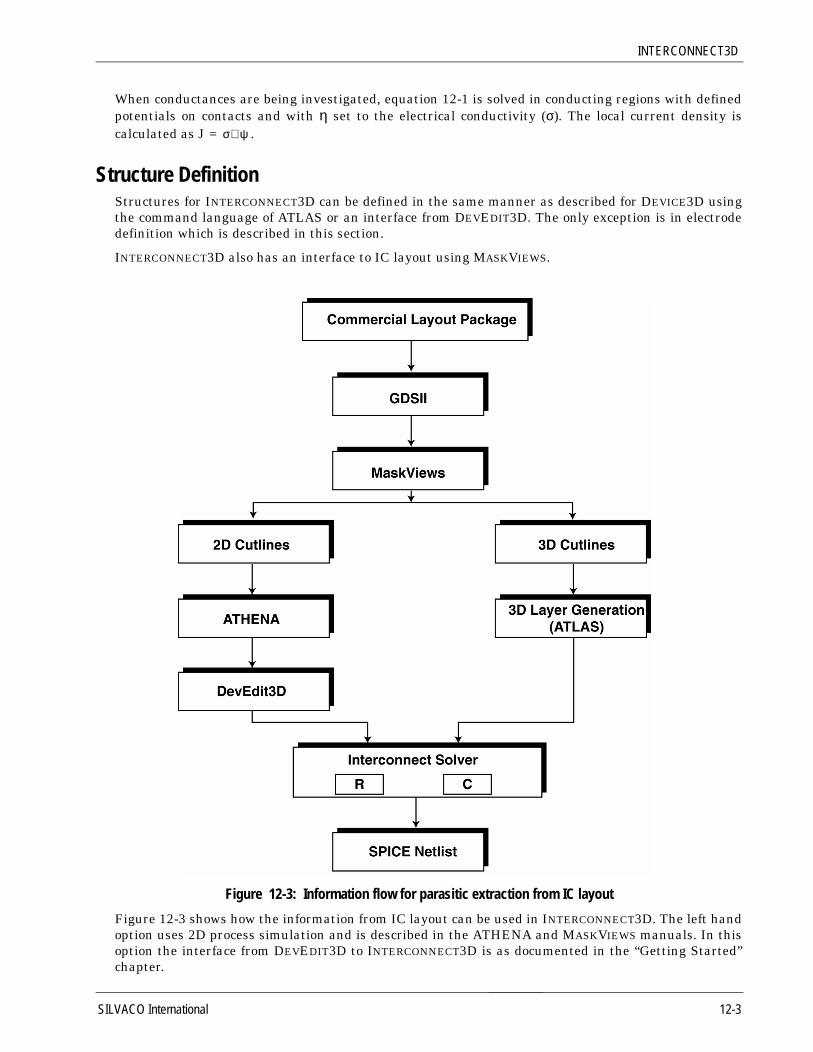
INTERCONNECT3D
When conductances are being investigated, equation 12-1 is solved in conducting regions with definedpotentials on contacts and with η set to the electrical conductivity (σ). The local current density iscalculated as J = .
Structure DefinitionStructures for INTERCONNECT3D can be defined in the same manner as described for DEVICE3D usingthe command language of ATLAS or an interface from DEVEDIT3D. The only exception is in electrodedefinition which is described in this section.
INTERCONNECT3D also has an interface to IC layout using MASKVIEWS.
Figure 12-3: Information flow for parasitic extraction from IC layout
Figure 12-3 shows how the information from IC layout can be used in INTERCONNECT3D. The left handoption uses 2D process simulation and is described in the ATHENA and MASKVIEWS manuals. In thisoption the interface from DEVEDIT3D to INTERCONNECT3D is as documented in the “Getting Started”chapter.
σ∇ψ
SILVACO International 12-3

ATLAS User’s Manual - Volume 2
The right hand branch of Figure 12-3 shows the direct layout to INTERCONNECT3D interface. This isdocumented below.
Tutorial For The MaskViews InterfaceThe MASKVIEWS-INTERCONNECT3D interface is a two step process. Firstly the mask data must beextracted and saved in MASKVIEWS. After this the layer structure of the interconnect is defined inATLAS.
Saving Mask Data For INTERCONNECT3D
The operation of MASKVIEWS including the GDS-II interface is described in the MASKVIEWSdocumentation. This tutorial assumes the layout has been correctly entered in to MASKVIEWS.
1. Set the simulator in MASKVIEWS to ATLAS. Use the Properties menu to change the simulator to ATLAS. Press Save if you want to have ATLAS as the default interface from MASKVIEWS.
2. Press the button Write_File on the main MASKVIEWS window.
3. Go to the top left of the area of your layout you wish to simulate. Press the left mouse key and hold it down. Drag the mouse over the area you wish to load into INTERCONNECT3D.
4. A new menu will appear with the coordinates of the box you have drawn.
5. Enter the name of a cross-section file (e.g.. myfile.sec)
6. Press Preview on this menu.
7. A graphics window will appear with the mask layout in 3-D. Use this to check that your chosen area is correct. The resolution of complex mask scan be controlled using the resolution setting under the MASKVIEWS menu: Define/Screen.
8. Press Write. A file is written to your disk. This file will be used in INTERCONNECT3D.
Loading Mask Data Into INTERCONNECT3D
The section of the layout file saved by MASKVIEWS should be loaded into ATLAS through the MESHstatement in the form
MESH NX=<INTEGER> NZ=<INTEGER> THREE.D LAYFILE=<FILENAME>
Note that the THREE.D parameter is required. The LAYFILE parameter specifies the name of the filesaved by MASKVIEWS. Most importantly, notice that the NY parameter is not specified on the MESHstatement. This is because the y-direction mesh is built up using the ADDLAYER statement.
The ADDLAYER statement makes a layer of the specified thickness in microns with the number of meshpoints in the y-direction specified by the DIVISION parameter.
ADDLAYER thick=<VALUE> mask=<layer_name> division=<INTEGER VALUE>
The MASK parameter tells ATLAS which mask to use from the MaskViews layout. The layer namemust correspond exactly with the layer name in MASKVIEWS.ATLAS assumes the drawn features aremetallic regions and the clear regions are insulator. If no MASK parameter is used, ATLAS assumes thelayer is completely formed from insulator.
Defining Electrodes Electrode specification in INTERCONNECT3D is different from other ATLAS simulations. Typicalstructures for INTERCONNECT3D consist of many metal conductors embedded in blocks of insulator.Some of the metal conductors are connected to make an interconnect. Each interconnect needs to be
12-4 SILVACO International
INTERCONNECT3D
defined by a unique electrode number or name. In INTERCONNECT3D, connectivity between conductorsis done automatically with no user intervention required.
There are several methods electrodes can be defined for INTERCONNECT3D:
• Define electrodes as usual in ATHENA, DEVEDIT3D or ATLAS. See ‘Getting Started’ fordetails. This method is typical if the DEVEDIT3D interface is used for conductance calculations.
• Do not define any electrodes. In this case the program finds connected blocks of metal for eachinterconnect. Each interconnect is assigned a different electrode number. The position of apoint in each conductor is printed to the run-time output to enable users to tell the number ofeach interconnect. This method is typical when the MASKVIEWS interface is used.
• Specify the point which is inside any conductor using the ELECTRODE statement.
ELECTRODE NUM=<integer> X.PNT=<val> Y.PNT=<<val> Z.PNT=<val>\
All the metal conductors of the interconnect structure connected to that point will assume the sameelectrode number. X.PNT and Z.PNT have no defaults, Y.PNT has a default of zero.
Specify parallelopiped, which intersects electrode, with boundaries (X.MIN,X.MAX)(Y.MIN,Y.MAX),(Z.MIN,Z.MAX), in the ELECTRODE statement; then all the connected points of interconnect structurewill refer to the same electrode.
ELECTRODE NUM=<integer> X.MIN=<val> Y.MIN=<val> Z.MIN=<val> \
X.MAX=<val> Y.MAX=<val> Z.MAX=<val>
In this case default values of these parameters differ from the usual ATLAS case. They are:
X.MIN - has no default; X.MAX - has no default; Y.MIN = 0; Y.MAX = <layer_thickness>; Z.MIN = 0; Z.MAX = 0;
SILVACO International 12-5

ATLAS User’s Manual - Volume 2
Model And Material Parameter Selection
Conductivity CalculationsIn conductivity calculations, the conductance of each region needs to be set using the GCOND parameterof the MATERIAL statement. For example:
MATERIAL REGION=2 GCOND=1.E3
To select that a conductance calculation is required the following statement is used:
MODEL EX.RES
Capacitance Calculations For capacitance calculation, the relative permittivity of insulator regions can be set using theMATERIAL statement. If the DEVEDIT3D interface is used this can be done using:
MATERIAL REGION=<integer> PERM=<value>
If the MASKVIEWS interface is used, INTERCONNECT3D assumes that all insulators are silicon dioxideand have a relative permittivity of 3.9. To override this, the MATERIAL statement is used. For exampleto set a nitride dielectric between two conductors in layers M1 and M2:
ADDLAYER MASK=M1 THICK=1.0 DIV=5 ADDLAYER THICK=1.0 DIV=5 ADDLAYER MASK=M2 THICK=1.0 DIV=5 MATERIAL LAYER=2 PERM=7.2
The value of the LAYER parameter is counted from the bottom upwards.
To select that a capacitance calculation is required the following statement should be included in thecommand file.
MODELS EX.CAP
12-6 SILVACO International
INTERCONNECT3D
Applying CD Variations and MisalignmentThe ADDLAYER statement supports the use of parameters to model variations in the interconnectstructure. The DELTA.CD.X and DELTA.CD.Z parameters are used to define a offset to the size ofany metal feature on that layer in the indicated direction. The units are microns. Negative values willincrease the metal width with the X or Z direction, positive values will decrease it.
Similarly the parameters MISALIGN.X and MISALIGN.Z are used to misalign layers relative to thepositions in the Maskviews section file. Separate misalignments in X and Z can be specified to modelthe worst case alignment of multi-layer interconnects. The default values are 0.0.
Numerical MethodsNo special numerical methods are required for either conductance or capacitance simulations. NoMETHOD statement is required.
Obtaining Solutions A solution is obtained for both capacitance and conductance modes with the simple statement:
SOLVE OUTF=<filename>
Only one SOLVE statement is allowed in each run of INTERCONNECT3D.
Interpreting the Results The output of INTERCONNECT3D simulation consist of a SPICE sub-circuit netlist of the capacitance orconductance of the structure. For capacitance calculations this is the capacitance between each pair ofconductors in Farads. For conductance calculations it is the resistance between each pair of electrodesin ohms.
The three dimensional structure and potential distribution can be saved in an output structure file bysetting the OUTFILE parameter in statement. This structure can be plotted using TONYPLOT3D.
More InformationExamples using INTERCONNECT3D have been installed on your distribution tape or CD. Moreinformation about the use of INTERCONNECT3D can be found by reading the text associated with eachexample.
SILVACO International 12-7

ATLAS User’s Manual - Volume 2
[This page intentionally left blank]
12-8 SILVACO International

Chapter 13:THERMAL3D
OverviewTHERMAL3D solves the steady-state heat equation to find the equilibrium temperature distribution inplanar and nonplanar three-dimensional structures. The user specifies the heat sinks and sources, andalso chooses from several temperature-dependent models for thermal conductivity within each region.A typical application for THERMAL3D is a package simulation for a power circuit or III-V ICs.
Before reading the following sections, users are advised to read the 3D device simulation chapter.
3D Structure GenerationTHERMAL3D supports structure defined on 3-D prismatic meshes. Structures may have arbitrarygeometries in two dimensions and consist of multiple slices in the third dimension. There are twomethods for creating a 3-D structure that can be used with THERMAL3D. One is through the commandsyntax of ATLAS, and the other through an interface to b. Please see documentation on both of thesemethods in the DEVICE3D chapter.
Defining Heat Sources
Heat sources are identified with regions in the 3D structure. Regions are defined in the mannerdocumented in the “Getting Started” and 3D device simulation chapters. A region has a uniquenumber, which is used to identify the region on the MATERIAL statement. The POWER parameter of theMATERIAL statement is used to set the power of the heat source in watts.
MATERIAL REGION=2 POWER=0.35
The POWER parameter must be set on the SOLVE statement if the user wishes to step the powerthrough a range of values. See the section “OBTAINING SOLUTIONS IN THERMAL3D” in this chapter forthe proper syntax.
Defining Heat Sinks
Heat sinks are identified as electrodes in the 3-D structure. Heat sink areas should be defined aselectrodes in the manner documented in the “Getting Started” and “3-D Device Simulation” chapters.Each electrode (heat sink) has a unique number, which is used to set the temperature on the heat sinkduring simulation. Setting the temperature of the heat sink is documented in the ‘Obtaining Solutions’section of this chapter.
SILVACO International 13-1
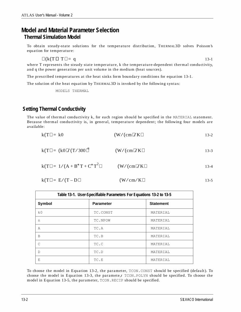
ATLAS User’s Manual - Volume 2
Model and Material Parameter SelectionThermal Simulation Model
To obtain steady-state solutions for the temperature distribution, THERMAL3D solves Poisson’sequation for temperature:
13-1where T represents the steady state temperature, k the temperature-dependent thermal conductivity,and q the power generation per unit volume in the medium (heat sources).
The prescribed temperatures at the heat sinks form boundary conditions for equation 13-1.
The solution of the heat equation by THERMAL3D is invoked by the following syntax:
MODELS THERMAL
Setting Thermal Conductivity The value of thermal conductivity k, for each region should be specified in the MATERIAL statement.Because thermal conductivity is, in general, temperature dependent; the following four models areavailable:
13-2
13-3
13-4
13-5
To choose the model in Equation 13-2, the parameter, TCON.CONST should be specified (default). Tochoose the model in Equation 13-3, the paramete,r TCON.POLYN should be specified. To choose themodel in Equation 13-5, the parameter, TCON.RECIP should be specified.
Table 13-1. User-Specifiable Parameters For Equations 13-2 to 13-5
Symbol Parameter Statement
k0 TC.CONST MATERIAL
n TC.NPOW MATERIAL
A TC.A MATERIAL
B TC.B MATERIAL
C TC.C MATERIAL
D TC.D MATERIAL
E TC.E MATERIAL
∇ k T(( )∇T ) q=
k T( ) k0= W cm( )⁄ K⁄( )
k T( ) k0( ) T 300⁄( )n⁄= W cm( )⁄ K⁄( )
k T( ) 1 A B∗T C∗++ T2( )⁄= W cm( )⁄ K⁄( )
k T( ) E T D–( )⁄= W cm⁄ K⁄( )
13-2 SILVACO International

THERMAL3D
Example
MATERIAL REGION=2 TCON.POWER TC.CO=1.0 TC.NPOW=1.2
means that the temperature-dependent thermal conductivity for region #2 is expressed as
13-6
Suggested Parameters For Thermal ConductivityThere are no pre-set material defaults in THERMAL3D. The following values are recommended forthermal conductivity of GaAs and Si.
For GaAs, use model B with
MATERIAL TCON.POWER TC.CO=0.44 TC.POW=1.25
For Si, use model B, C, or D with
(model B)MATERIAL TCON.POWER TC.CO=1.55 TC.POW=-1.33 (model C)MATERIAL TCON.POLYN TC.A=0.03 TC.B=1.56e-3 TC.C=1.65e-6 (model D)MATERIAL TCON.RECIP TC.E=320 TC.D=80
Numerical MethodsNo special numerical methods are required for thermal simulation. A METHOD statement with noparameters is assumed by default.
Obtaining Solutions In THERMAL3DThe SOLVE statement in used in THERMAL3D for heat-flow solutions much the same as it is used inother ATLAS simulations involving electrical biases. The temperature in kelvin on each heat sink isused to prescribe the boundary condition temperatures. For example,
SOLVE T1=300 T2=500
sets the temperature at 300 K and 500 K on heat sink #1 and #2 respectively.
Multiple SOLVE statements are allowed in THERMAL3D. This is useful for obtaining solutions forseveral combinations of heat sinks and thermal power sources. A range of solutions can also beobtained by stepping the value of a heat sink or power source. For example,
SOLVE T1=300 POWER2=0.35 POWER3=0.4 NSTEPS=5 STEPREGION=3 \ POWERFINAL=0.8 OUTFILE=thermal_out0
increments the thermal power source in region #3 from 0.4 watts to 0.8 watts in 5 steps and:
SOLVE T1=300 POWER2=0.35 NSTEPS=3 ELECTRODE=1 \TEMPFINAL=600 OUTFILE=thermal_out0
increments the temperature on electrode #1 from 300 K to 600 K in 3 steps. Thermal power andtemperature can be simultaneously sweep.
If more than one region power is specified during a sweep, the region to be stepped must be specifiedby STEPREGION=# as shown in the first example above. If the STEPREGION parameter is not specified,the smallest numerical value of POWER# is stepped.
During temperature and power sweeps, the output filename is modified according to the followingrule: The rightmost character is incremented using the sequence 0-9, A-Z, a-z. When a character isincremented beyond ‘z’ the character is set to ‘0’> and the character to the left (smaller than ‘z’) isincremented.
K T( ) 1
T 300⁄( )1.2---------------------------=
SILVACO International 13-3

ATLAS User’s Manual - Volume 2
Complete syntax information for the SOLVE statement can be found in Chapter 15, “Statements”.
The SOLVE statement is used in THERMAL3D for heat flow solutions much as it is used in other ATLASsimulations for electrical biases. The temperature in Kelvin on each heat sink in the device must be seton the SOLVE statement. The parameter, Tn, where n is the number of the heat sink, is used to set thetemperature. For example:
SOLVE T1=300 T2=500
This sets 300K on heat sink #1 and 500K on heat sink #2. Only one SOLVE statement is allowed inany THERMAL3D input file.
Interpreting The Results From THERMAL3DThe output of thermal simulation consists of the minumum and maximumcalculated temperature ofeach region and its location. The three-dimensional temperature distribution can be saved in an ouputstructure file by setting the OUTFILE parameter in the SOLVE statement and visualized usingTONYPLOT3D.
The output of thermal simulation consist of the minimum and maximum calculated temperature ofeach region and its location. The three dimensional temperature distribution can be saved in a outputstructure file by setting the OUTFILE parameter in the SOLVE statement and visualized usingTONYPLOT3D.
More InformationMany examples using THERMAL3D have been installed on your distribution tape or CDROM. Moreinformation about the use of THERMAL3D can be found by reading the text associated with eachexample.
13-4 SILVACO International
Chapter 14:Numerical Techniques
OverviewThis chapter describes the overall process of obtaining a numerical solution, the subtasks involved,and the options and defaults available in ATLAS.
Users do not need to master this material in order to use ATLAS. Chapter Two presents theinformation about numerical techniques that is needed by most users. This chapter providesadditional information that will mainly be of interest to advanced users.
Numerical Solution ProceduresSemiconductor device operation is modeled in ATLAS by a set of anywhere from one to six coupled,non-linear, partial differential equations (PDEs). ATLAS produces numerical solutions of theseequations by calculating the values of unknowns on a mesh of points within the device. An internaldiscretization procedure converts the original, continuous model to a discrete non-linear algebraicsystem that has approximately the same behavior. The set of PDEs, the mesh and the discretizationprocedure determine the non-linear algebraic problem that must be solved.
The non-linear algebraic system is solved using an iterative procedure that refines successiveestimates of the solution. Iteration continues until the corrections are small enough to satisfyconvergence criteria, or until it is clear that the procedure is not going to converge. The non-lineariteration procedure starts from an initial guess. The corrections are calculated by solving linearizedversions of the problem. The linear subproblems are solved by using direct techniques or iteratively.
Different solution procedures exhibit different behavior with respect to convergence, accuracy,efficiency, and robustness. The two main aspects of convergence are whether a solution is obtained,and if so, how rapidly it is approached. Accuracy is how closely the computed solution approximatesthe true solution. Efficiency is the time required to produce a solution. Robustness is the ability toconverge for a wide range of structures, using meshes and initial guess strategies that are notoptimum.
When solving general systems of non-linear equations there are no guarantees that any particularmethod will always work. It is also the case that different methods can work better for differentproblems. Fortunately there is now a lot of practical experience concerning the numerical techniquesthat are effective for device simulation. This practical experience has been captured in ATLAS in theform of default methods and parameters that work well in almost all circumstances. This chapterprovides advanced information of interest to users who want to change the defaults.
MeshesThe specification of meshes involves a trade-off between the requirements of accuracy and numericalefficiency. Accuracy requires a fine mesh that can resolve all significant features of the solution.Numerical efficiency requires a coarse mesh that minimizes the total number of grid points. Thistrade-off between accuracy and numerical efficiency is frequently a source of problems for beginners.Fortunately, enough experience to define reasonable meshes is soon acquired.
ATLAS uses triangular meshes. Some triangulations yield much better results than others. Meshgeneration is still an inexact science, but guidelines and heuristics for defining satisfactory meshesexist. ‘Good’ triangulations have the following features:
• They contain enough points to provide the required accuracy.
• They do not contain too many unnecessary points that impair efficiency.
SILVACO International 14-1

ATLAS User’s Manual - Volume 2
• They avoid, or at least minimize, the number of obtuse triangles. Obtuse triangles tend to impairaccuracy, convergence, and robustness.
• They avoid, or at least minimize, the number of long, thin triangles. These triangles also tend toimpair accuracy, convergence, and robustness.
• They allow the average size of triangles to change smoothly in transition from a region wherevery small triangles must be used to a region where the use of much larger triangles isacceptable.
The error associated with a mesh can be investigated systematically by repeating a calculation using asequence of finer meshes. This is very time consuming and is hardly ever done. The typical approach isto adequately resolve structural features, including doping, with an initial or base mesh, and then addnodes as required to resolve significant features of the solution. The insertion of additional nodes(regridding) is normally done by the program, using criteria specified by the user.
The initial mesh used by ATLAS can be specified in several ways: it can be "inherited" from ATHENA,it can be constructed using DEVEDIT, or it can be specified using the ATLAS command language.Meshes can be refined using ATLAS commands, or using DEVEDIT. The remainder of this section willfocus on the capabilities available using ATLAS commands. The capabilities provided by DEVEDIT aredocumented in the VWF INTERACTIVE TOOLS manual.
There are limits on the maximum number of nodes that can be specified. Two-dimensional ATLASsimulations may have up to 9,600 nodes. Three-dimensional simulations may have up to 200,000nodes, 400,000 elements, with no more than 20,000 in a single plane and a maximum of 200 planes inthe z direcction. Most devices can be adequately simulated in two dimensions using meshes thatcontain from several hundred to around 3000 nodes.
Mesh RegriddingThe REGRID statement supports refinement of regions of the mesh according to specified criteria.Refinement can occur when a specified solution variable exceeds some value, or when the change inthat variable across a triangle exceeds a value. The variable can be any of the key quantities in aproblem, such as potential, carrier concentration, doping concentration, or electric field.
The regrid algorithm searches the initial grid for triangles that meet the criterion specified forrefinement. Each triangle that is identified is divided into four congruent subtriangles. Grid quantities(doping, potential, carrier concentrations, and so forth) are interpolated onto the new nodes, usinglinear or logarithmic interpolation, as appropriate for that quantity. The initial grid is referred to asbeing "on level 0" and the new triangles are referred to as "on level 1". After all level 0 triangles havebeen examined, the same procedure is applied to level 1 triangles, and any subtriangles of level 1become "level 2"> triangles. The grid is checked for consistency at each level and is updated to avoidabrupt changes of size from one triangle to the next. The regrid process continues until no moretriangles meet the refinement criteria, or until a specified maximum level of refinement is reached.Grids used in practice are often coarser than is required to meet desirable refinement criteria, and sothe maximum level is the key factor in determining the size of the grid after refinement.
The MAX.LEVEL parameter of the REGRID statement is used to limit the amount of refinement at eachstep. By default, ATLAS sets the maximum level equal to one more than the highest level in theexisting mesh. To update a coarse region without regridding the finer regions, after a mesh hasalready been refined several times, set the maximum level below the level of the finer regions in theexisting grid.
If several levels of regrid are performed in immediate succession, interpolated data is used to make therefinement decisions at higher levels. Since semiconductor problems are non-linear, this interpolationmay not produce satisfactory results. It is often a good idea to calculate a new solution between regridoperations, i.e. to regrid only one level at a time and obtain a new solution each regrid operation.
Two popular choices of quantities to be used for mesh refinement are potential and doping. Ideally,variations of electrostatic and quasi-Fermi potentials across an element would be limited to no more
14-2 SILVACO International

Numerical Techniques
than kT/q, and variations in doping would be no more than a factor of 5 or so. In practice therefinement criteria are often significantly coarser: around 10-20 kT/q for potential, and two to threeorders of magnitude for doping. In high level injection situations, it is a good idea to regrid when thevalue of minority carrier concentration exceeds the local doping concentration.
Mesh Smoothing Although every step of grid generation can introduce obtuse triangles, two steps in particular cancause problems. The first is that distorting a rectangular mesh introduces a very large number ofobtuse elements. The second is that when regridding a rectangular grid that contains triangles withan aspect ratio of 4:1 or greater, very obtuse triangles are created in the transition region betweenhigh and low grid density. The REGRID statement allows several procedures to be used when dealingwith poorly shaped elements such as obtuse triangles.
The two techniques are node smoothing and triangle smoothing. With node smoothing, severaliterative passes are carried out during which each node is moved to a position which improves theangles of the triangles surrounding it. Node smoothing should only be used for grids that are alreadyirregular. If node smoothing is used for nearly rectangular grids, it may significantly degrade thequality of the mesh.
With triangle smoothing (which is also referred to as diagonal flipping), each adjoining pair oftriangles is examined. If appropriate, the diagonal of the quadrilateral is flipped to stabilize thediscretization. The diagonal is never flipped when two elements are composed of different materials.When elements are of the same material but have different region numbers, the user can specifywhether or not to flip the diagonals.
Triangle smoothing is desirable in almost all cases, and should be performed on both the initial gridand on subsequent regrids. The only exception to this rule arises from a undesirable interaction ofthree elements: regrid, high aspect ratio triangles, and smoothing. This situation frequently occurs ingate oxide regions that involve long, thin triangles. In these cases, smoothing may produce largetriangles surrounded by many smaller triangles, giving the appearance of a hole in the mesh. Toovercome this, the smoothing command SMOOTH=4 can be used to limit the formation of the largetriangles.
Discretization
The Discretization ProcessThe discretization process yields relationships between the variables defined at mesh points. In orderto be useful, a discretization must be consistent, i.e. it must limit to the underlying equation in thelimit that the mesh size tends to zero. All of the discretizations used in ATLAS have this property.Different discretizations can have different properties with respect to accuracy. The most importantmeasure of accuracy is the order of the scheme, i.e. how errors scaled as the difference between meshpoints tends to zero. Discretization schemes used in device simulation are often second order, i.e. asthe mesh becomes very fine the discretization error varies as the square of the separation betweenmesh points.
The discretizations implemented in ATLAS use the box integration method to approximate differentialoperators on a general triangular grid. Each equation is integrated over a small polygon whichencloses each node. The set of all polygons completely covers the solution domain. The integrationprocedure equates fluxes into a polygon with sources and sinks inside the polygon, which means thatquantities that are conserved physically are also conserved by the numerical solution.
The fluxes must be discretized carefully for the carrier continuity and energy balance equations,otherwise nonphysical oscillations and negative carrier concentrations and temperatures may arise.Scharfetter and Gummel35 introduced approximations for current densities that overcome this
SILVACO International 14-3

ATLAS User’s Manual - Volume 2
problem. Generalizations of this approach are used in ATLAS for the discretization of current densitiesand energy fluxes.
Non-Linear IterationThe non-linear solution method, and associated parameters such as iteration and convergence criteria,are specified in the METHOD statement. Non-linear iteration solution methods are specified in theMETHOD statement using the parameters NEWTON, GUMMEL, or BLOCK. Combinations of theseparameters may also be specified. In order to understand the effect of these parameters, it is helpful tobriefly review how numerical solutions are obtained.
The non-linear algebraic system that results from discretization on a mesh is solved iterativelystarting from an initial guess. Linearized subproblems are set up and solved. These providecorrections that are used to update the current estimate of the solution. Different sequences of linearsubproblems correspond to different non-linear iteration strategies. Iteration continues untilconvergence criteria are met, in which case the solution is accepted; or until a preset maximumallowable number of iterations is reached, in which case a different technique is tried or the solutionprocedure is abandoned. When a solution fails to converge, a user normally tries a different grid, adifferent initial guess strategy, or a different non-linear iteration technique.
Newton IterationEach iteration of the Newton method solves a linearized version of the entire non-linear algebraicsystem. The size of the problem is relatively large, and each iteration takes a relatively long time.However, the iteration will normally converge quickly (in about three to eight iterations) so long as theinitial guess is sufficiently close to the final solution. Strategies that use automatic bias step reductionin the event of non-convergence loosen the requirement of a good initial guess. Newton’s method is thedefault for drift-diffusion calculations in ATLAS. There are several calculations for which ATLASrequires that Newton’s method is used. These are: DC calculations that involve lumped elements;transient calculations; curve tracing; and when frequency-domain small-signal analysis is performed.
The Newton-Richardson method is a variant of the Newton iteration that calculates a new version ofthe coefficient matrix only when slowing convergence demonstrates that this is necessary. Anautomated Newton-Richardson method is available in ATLAS, and improves performance significantlyon most problems. The automated Newton-Richardson method is enabled by specifying the AUTOparameter of the METHOD statement.
If convergence is obtained only after many Newton iterations, the problem is almost certainly poorlydefined. The grid may be very poor (i.e. it contains many obtuse or high aspect ratio triangles), or adepletion region may have extended into a region defined as an ohmic contact, or the initial guess maybe very poor.
Gummel IterationEach iteration of Gummel’s method solves a sequence of relatively small linear subproblems. Thesubproblems are obtained by linearizing one equation of the set with respect to its primary solutionvariable, while holding other variables at their most recently computed values. Solving this linearsubsystem provides corrections for one solution variable. One step of Gummel iteration is completedwhen the procedure has been performed for each independent variable. Gummel iteration typicallyconverges relatively slowly, but the method will often tolerate relatively poor initial guesses. TheGummel algorithm can not be used with lumped elements or current boundary conditions
Two variants of Gummel’s method can improve its performance slightly. These both limit the size ofthe potential correction that is applied during each Gummel loop. The first method, called damping,truncates corrections that exceed a maximum allowable magnitude. It is used to overcome numericalringing in the calculated potential when bias steps are large (greater than 1V for room temperaturecalculations). The maximum allowable magnitude of the potential correction must be carefully
14-4 SILVACO International

Numerical Techniques
specified: too small a value slows convergence, while too large a value can lead to overflow. TheDVLIMIT parameter of the METHOD statement is used to specify the maximum allowable magnitude ofthe potential correction. By default the value of this parameter is 0.1 V. Thus, by default Gummeliterations are dampped. To specify undamped Gummel iterations, the user should specify DVLIMIT tobe negative of zero.
The second method limits the number of linearized Poisson solutions per Gummel iteration, usually toone. This leads to under-relaxation of the potential update. This “single-Poisson” solution modeextends the usefulness of Gummel’s method to higher currents. It can be useful for performing lowcurrent bipolar simulations, and simulating MOS transistors in the saturation region. It is invoked byspecifying the SINGLEPOISSON parameter of the METHOD statement.
Block IterationATLAS offers several block iteration schemes that are very useful when lattice heating or energybalance equations are included. Block iterations involves solving subgroups of equations in varioussequences. The subgroups of equations used in ATLAS have been established as a result of numericalexperiments that established which combinations are most effective in practice.
In nonisothermal drift-diffusion simulation, specifying the BLOCK method means that Newton’smethod is used to update potential and carrier concentrations, after which the heat flow equation issolved in a decoupled step.
When the carrier temperature equations are solved for a constant lattice temperature, the BLOCKiteration algorithm uses Newton’s method to update potential and concentrations. The carriertemperature equation is solved simultaneously with the appropriate continuity equation to update thecarrier temperature and again carrier concentration.
When both the heat flow equation and the carrier temperature equations are included, the BLOCKscheme proceeds as described previously for the carrier temperature case, and then performs onedecoupled solution for lattice temperature as a third step of each iteration.
Combining The Iteration MethodsIt is possible to start with the GUMMEL scheme and then switch to BLOCK or NEWTON if convergence isnot achieved within a certain number of iterations. One circumstance where this can be very helpful isthat Gummel iteration can refine initial guess to a point from which Newton iteration can converge.The number of initial GUMMEL iterations is limited by GUM.INIT.
It can also be desirable to use BLOCK iteration and then switch to NEWTON if convergence is notachieved. This is the recommended strategy for calculations that include lattice heating or energybalance. The number of initial BLOCK iterations is limited by NBLOCKIT
Any combination of the parameters GUMMEL, BLOCK and NEWTON may be specified on the METHODstatement. ATLAS will start with GUMMEL if it is specified. If convergence is not achieved within thespecified number of iterations, it will then switch to BLOCK if BLOCK is specified; if convergence is stillnot achieved the program will then switch to NEWTON.
Solving Linear SubproblemsThe linear subproblems generated by non-linear iteration can be solved by direct or iterative methods.Direct methods produce solutions in a predictable number of arithmetic operations. Solutions areaffected by roundoff error, but are otherwise exact. Iterative methods obtain solutions by making aseries of corrections to an initial guess. Iteration proceeds until the calculated corrections satisfyspecified convergence criteria. The results are not exact to within roundoff error, and convergence isnot guaranteed for general problems. However, iterative methods can be more efficient than directmethods for large linear systems, and generally require less memory.
SILVACO International 14-5

ATLAS User’s Manual - Volume 2
There are mathematical proofs regarding the types of linear system for which iterative techniquesconverge. All common iterative schemes converge for linear systems that are symmetric positivedefinite (SPD). The linearized form of Poisson’s equation is of this type. The continuity equations arenot SPD, but they can be reliably solved by modern, advanced iterative methods.
The size and structure of the coefficient matrix of the linear system plays an important role in thechoice of direct or iterative methods. The overall problem size is determined by the number ofvariables per node (m) and the number of nodes (n). The number of unknowns is m x n. The linear subproblems associated with Newton iteration have a coefficient matrix with (m x n)2 elements. Eachlinearized subproblem which is used in Gummel iteration has a coefficient matrix with n2 elements.
For practical 2-D device simulation problems, the number of elements in the coefficient matrix istypically between 105 and 108. Fortunately the matrices are sparse, i.e. most of the entries are zero,and need not be stored explicitly. The sparsity arises because the variables at each node are coupled toonly a few neighboring nodes. Special direct techniques are available for solving sparse matrices.
Direct techniques are preferred for relatively small problems. They provide reliable solutions that areexact to within roundoff error in a time that is predictable. Iterative techniques are preferred for verylarge problems because they are faster and require less memory. Direct techniques for solving sparsematrices have a competitive performance for the problem sizes typically encountered in 2-D devicesimulation, and are used by ATLAS to solve most of the linear subproblems that arise.
Convergence Criteria for Non-linear IterationsAfter a few non-linear iterations, the errors will generally decrease at a characteristic rate as theiteration proceeds. Non-linear iteration techniques typically converge at a rate that is either linear orquadratic. The error decreases linearly when Gummel iteration is used, i.e. it is reduced by about thesame factor at each iteration. For Newton iteration the convergence is quadratic, i.e., small errors lessthan one are approximately squared at each iteration. The non-linear iteration is terminated when theerrors are acceptably small. The conditions required for termination are called convergence criteria.Much effort has gone into developing reliable default convergence criteria for ATLAS. The defaultparameters work well for nearly all situations, and most users will never need to change them.
Error Measures A single positive number that characterizes error is obtained by taking a norm of the errors associatedwith each unknown. The quantity that ATLAS tries to reduce to zero is the difference between the leftand right hand sides of the equation. It is natural to use this quantity as the measure of the error. Theassociated error norm is called the right hand side (RHS) norm. The units of the RHS norm are C/µmfor the Poisson equation, and A/µm for the continuity equations.
Carrier Concentrations and CLIM.DD (CLIMIT)
Another measure of error is provided by the size of the calculated corrections for each unknown. Sincethe updates are the unknown “xs” at each step, this is called the X norm. Potential updates aremeasured in units of kT/q. Updates to carrier concentrations are measured relative to the previousvalue at the point. This relative error (εC) is defined as:
14-1
where:
C = n or p, for electrons and holes respectively.
m is the node identifier.
εC max
m
CmK 1+
CmK
–
max C0 CmK,( )
--------------------------------=
14-6 SILVACO International

Numerical Techniques
C0 is a characteristic concentration.
K is the iteration number
C0 is specified as or as CLIM.DD or as CLIM·c*,
CLIM.DD = CLIMT·c*. 14-2where:
14-3
CLIM.DD (or CLIMIT) is specified in the METHOD statement.
It is difficult to specify a reasonable default value for the parameter CLIM.DD in all situations. Inmany difficult cases, the round-off numerical errors do not allow for the resolution of very lowconcentrations. The default value of CLIMIT is set at 104 (the corresponding default value for CLIM.DDin Silicon i s 4.5·1013cm-3). In simulation of breakdown, a lower value of CLIM.DD (~108cm-3 forSilicon diodes) should be specified; otherwise, a “false” solution may be obtained.
Discussion of CLIM.EB
To estimate errors in the lattice temperature equation and the energy balance equations,corresponding RHS norms and X norms are calculated in ATLAS. Updates to temperature aremeasured relative to some characteristic value of temperature. The parameter CLIM.EB, can beviewed as a regularization parameter for the case of very small electron or hole densities in the energybalance equations. The CLIM.EB parameter specifies the minimum value of concentration for whichthe relaxation term in the energy balance equation will be properly resolved. The temperatures forpoints where the concentration is much less than CLIM.EB are equal to the lattice temperature. Theunits of CLIM.EB are cm-3 and the default is 0.0.
Terminal Current Criteria
Another qualification for convergence is derived from the relative changes in terminal currents andthe satisfaction of total current conservation. This qualification can be expressed as the simultaneoussatisfaction of the following conditions:
14-4
and
< 0.01 maxi
14-5where
Ii is the current through contact i
K is the iteration number
E1 and E2 are specified tolerances
nc is the number of contacts
c∗ NcNv4=
IiK 1+
IiK
– E1≤ IiK 1+
E2+
ΣIiK 1+
IiK 1+
E2,( )
I 1 nc,=
SILVACO International 14-7

ATLAS User’s Manual - Volume 2
Summary of Termination Criteria A summary of the termination criteria that is enough for most purposes will now be given. Detailedreference information is provided in the next section.
The non-linear iteration is terminated when one of the following four criteria is satisfied.
1. The X norm for every equation falls below a specified tolerance. The specified tolerances for X norms are:
- for potential equation;
- for concentration equations;
- for lattice temperature equation;
- for carrier temperature equation.
2. The RHS for all equations and X norms for energy balance falls below a specified tolerance. The specific tolerances are:
- for potential equations;
- for concentration equations;
- for lattice temperature equations;
-for carrier temperature equations.
3. For every equation either the X norm or the RHS norm falls below a specified tolerance. In this case, both the XNORM and RHSNORM parameters must be specified true.
4. If either 1. or 2. or 3. criterion is fulfilled for weaker values of tolerances, i.e. for specified tolerances multiplied by the parameter W, and current criteria 14-4 and 14-5 are satisfied.
To exclude the X-norm criterion, ^XNORM should be specified in the METHOD statement; to exclude RHS-norm criterion, ^RHSNORM should be specified; to exclude the current criterion E1 and E2 should bemade very small. All the above mentioned tolerances can be changed simultaneously by specifying therelaxation factor TOL.RELAX in the METHOD statement.
Ptolx
Ctolx
TLtolx
TCtolx
Ptolr
Ctolr
TLtolr
TCtolr
14-8 SILVACO International

Numerical Techniques
Table 14.1. User-Specifiable Parameters for Convergence Criteria
Symbol Statemen Parameter Default
METHOD PX.TOL 10-5
METHOD CX.TOL 10-5
METHOD TLX.TOL 10-5
METHOD TCX.TOL 10-5
METHOD PR.TOL 5.0x10⁻²⁶
METHOD CR.TOL 5.0x10⁻¹⁸
METHOD TLG.TOL 100
METHOD TCR.TOL 100
E1 METHOD IX.TOL 2.0x10⁻⁵
E2 METHOD IR.TOL 5.0x10⁻¹⁵
W METHOD WEAK 200
TOL.RELAX
METHOD TOL.RELAX 1
XNORM METHOD XNORM TRUE
RHSNORM METHOD RHSNORM TRUE
CLIMIT METHOD CLIMIT 104
CLIM.DD METHOD C0 4.5x10¹³
CLIM.EB METHOD CLIM.EB 0
Ptolx
Ctolx
TLtolx
TCtolx
Ptolr
Ctolr
TLtolr
TCtolr
SILVACO International 14-9

ATLAS User’s Manual - Volume 2
Detailed Convergence CriteriaOnly in very difficult situations is more detailed information concerning error estimation and thespecification of convergence criteria needed. The material is organized by algorithm.
Convergence Criteria For Gummel’s Algorithms
Relative update errors are defined as follows:
for potential
14-6
where mmax is the node where has its maximum value;
For electrons:
14-7
For holes:
14-8
For lattice temperature:
14-9
where nmax is the node where has its maximum value;
For carrier temperature:
14-10
where
14-11
εv
maxm
ϕmK 1+ ϕm
K–
max 1 ϕmmaxK 1+,( )
--------------------------------------------,=
ϕmK 1+ ϕm
K–
εn
maxm
nmK 1+
nmK
–
max C0 nmK,( )
-------------------------------------------=
εp
maxm
pmK 1+
pmK
–
max C0 PmK,( )
-------------------------------------------=
εTL
TL( )nmaxK 1+
TL( )nmaxK
–
TL( )nmaxK 1+
-------------------------------------------------=
TL( )iK 1+
εTcmax εTn
εTp,( )=
εTn
maxm Tn( )m
K 1+Tn( )m
K–
maxm
Tn( )mK 1+
----------------------------------------------------------=
14-10 SILVACO International
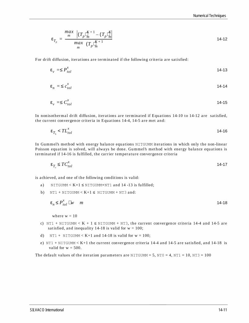
Numerical Techniques
14-12
For drift diffusion, iterations are terminated if the following criteria are satisfied:
14-13
14-14
14-15
In nonisothermal drift diffusion, iterations are terminated if Equations 14-10 to 14-12 are satisfied,the current convergence criteria in Equations 14-4, 14-5 are met and:
14-16
In Gummel’s method with energy balance equations NITGUMM iterations in which only the non-linearPoisson equation is solved, will always be done. Gummel’s method with energy balance equations isterminated if 14-16 is fulfilled, the carrier temperature convergence criteria
14-17
is achieved, and one of the following conditions is valid:
a) NITGUMM < K+1 ≤ NITGUMM+NT1 and 14 -13 is fulfilled;
b) NT1 + NITGUMM < K+1 ≤ NITGUMM + NT3 and:
14-18
where w = 10
c) NT1 + NITGUMM < K + 1 ≤ NITGUMM + NT3, the current convergence criteria 14-4 and 14-5 aresatisfied, and inequality 14-18 is valid for w = 100;
d) NT1 + NITGUMM < K+1 and 14-18 is valid for w = 100;
e) NT1 + NITGUMM < K+1 the current convergence criteria 14-4 and 14-5 are satisfied, and 14-18 isvalid for w = 500.
The default values of the iteration parameters are NITGUMM = 5, NT0 = 4, NT1 = 10, NT3 = 100
εTp
maxm Tp( )m
K 1+Tp( )m
K–
maxm
Tp( )mK 1+
----------------------------------------------------------=
εv P≤ tolx
=
εn c≤ tolx
=
εv C≤ tolx
=
εTLTLtol
x<
εTcTCtol
x≤
εn Ptolx
w m⋅≤
SILVACO International 14-11

ATLAS User’s Manual - Volume 2
Convergence Criteria For Newton’s Algorithm
Relative update errors are defined as follows:
For potential
14-19
For electron concentration:
14-20
For hole concentration:
14-21
For lattice temeprature and carrier temperature:
14-22
14-23
14-24
where the scaling temperature Tscale is by default equal to 300K.
To define the RHS norms used in ATLAS, first represent the non-linear equations obtained afterdiscretization at every node as
14-25
where α can be ψ, n, p, TL, Tn and Tp for the potential equation, electron continuity equation, holecontinuity equation, lattice temperature equation, electron temperature equation and hole
temperature equation, respectively. represents the vector of unknowns.
εvmax
mϕm
K 1+ ϕmK
–=
εn
maxm
nmK 1+
nmK
–
max C0 nmK,( )
---------------------------------------=
εp
maxm
pmK 1+
pmK
–
max C0 pmK,( )
---------------------------------------=
εTL
maxm TL( )m
K 1+TL( )– m
K
Tscale-----------------------------------------------------------,=
εTn
maxm Tn( )m
K 1+Tn( )– m
K
Tscale-----------------------------------------------------------,=
εTp
maxm Tp( )m
K 1+Tp( )– m
K
Tscale-----------------------------------------------------------,=
( ) χ( ) 0=
χ
14-12 SILVACO International

Numerical Techniques
The RHS norms in ATLAS is then defined as follows:
For the potential equation:
14-26
For the electron and continuity equations:
14-27
14-28
where CT = 10-4
For the lattice temperature and carrier temperature equations:
14-29
. 14-30
14-31
Newton iterations are terminated if one of the following criteria is satisfied:
a) the parameter XNORM is true and:
14-32
14-33
14-34
14-35
14-36
14-37
where w = 1
εvg max
m Fϕ=
εng max
mFn CT⋅=
εpg max
mFp CT⋅=
NcNv4 kT
εTL
g maxm FTL
=
εTn
g maxm FTn
=
εTp
g maxm FTp
=
εv Ptolx
w,⋅≤
εn ctolx
w,⋅≤
εp Ptolx
w,⋅≤
εTLTLtol
xw,⋅≤
εTnTCtol
xw,⋅≤
εTpTLtol
xw,⋅≤
SILVACO International 14-13
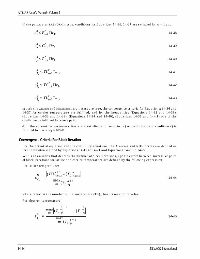
ATLAS User’s Manual - Volume 2
b) the parameter RHSNORM is true, conditions for Equations 14-36, 14-37 are satisfied for w = 1 and:
14-38
14-39
14-40
14-41
14-42
14-43
c) both the XNORM and RHSNORM parameters are true, the convergence criteria for Equations: 14-36 and14-37 for carrier temperature are fulfilled, and for the inequalities (Equations 14-32 and 14-38),(Equations 14-33 and 14-39), (Equations 14-34 and 14-40), (Equations 14-35 and 14-41) one of theconditions is fulfilled for every pair.
d) if the current convergence criteria are satisfied and condition a) or condition b) or condition c) isfulfilled for: w = w1 = WEAK
Convergence Criteria For Block Iteration
For the potential equation and the continuity equations, the X norms and RHS norms are defined asfor the Newton method by Equations 14-19 to 14-21 and Equations 14-26 to 14-27.
With s as an index that denotes the number of block iterations, update errors between successive pairsof block iterations for lattice and carrier temperature are defined by the following expression:
For lattice temperature:
14-44
where mmax is the number of the node where (TL)m has its maximum value.
For electron temperature:
14-45
εvg
Ptolr
w1,⋅≤
εng
Ctolr
w1,⋅≤
εpg
Ptolr
w1,⋅≤
εTL
gTLtol
rw1,⋅≤
εTn
gTCtol
rw1,⋅≤
εTp
gTLtol
rw1,⋅≤
εTL
B1T( )Lnmax
s 1+TL( )nmax
s–
maxm TL( )m
s 1+-----------------------------------------------------=
εTn
B1
maxm Tn( )m
s 1+
Tn( )– m
s
maxm Tn( )m
s 1+-------------------------------------------------------------=
14-14 SILVACO International
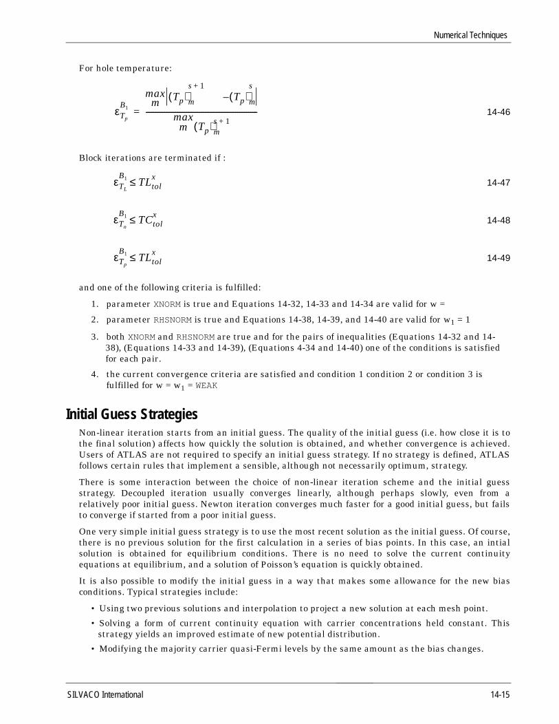
Numerical Techniques
For hole temperature:
14-46
Block iterations are terminated if :
14-47
14-48
14-49
and one of the following criteria is fulfilled:
1. parameter XNORM is true and Equations 14-32, 14-33 and 14-34 are valid for w =
2. parameter RHSNORM is true and Equations 14-38, 14-39, and 14-40 are valid for w1 = 1
3. both XNORM and RHSNORM are true and for the pairs of inequalities (Equations 14-32 and 14-38), (Equations 14-33 and 14-39), (Equations 4-34 and 14-40) one of the conditions is satisfied for each pair.
4. the current convergence criteria are satisfied and condition 1 condition 2 or condition 3 is fulfilled for w = w1 = WEAK
Initial Guess StrategiesNon-linear iteration starts from an initial guess. The quality of the initial guess (i.e. how close it is tothe final solution) affects how quickly the solution is obtained, and whether convergence is achieved.Users of ATLAS are not required to specify an initial guess strategy. If no strategy is defined, ATLASfollows certain rules that implement a sensible, although not necessarily optimum, strategy.
There is some interaction between the choice of non-linear iteration scheme and the initial guessstrategy. Decoupled iteration usually converges linearly, although perhaps slowly, even from arelatively poor initial guess. Newton iteration converges much faster for a good initial guess, but failsto converge if started from a poor initial guess.
One very simple initial guess strategy is to use the most recent solution as the initial guess. Of course,there is no previous solution for the first calculation in a series of bias points. In this case, an intialsolution is obtained for equilibrium conditions. There is no need to solve the current continuityequations at equilibrium, and a solution of Poisson’s equation is quickly obtained.
It is also possible to modify the initial guess in a way that makes some allowance for the new biasconditions. Typical strategies include:
• Using two previous solutions and interpolation to project a new solution at each mesh point.
• Solving a form of current continuity equation with carrier concentrations held constant. Thisstrategy yields an improved estimate of new potential distribution.
• Modifying the majority carrier quasi-Fermi levels by the same amount as the bias changes.
εTp
B1
maxm Tp( )m
s 1+
Tp( )– m
s
maxm Tp( )m
s 1+-------------------------------------------------------------=
εTL
B1 TLtolx≤
εTn
B1 TCtolx≤
εTp
B1 TLtolx≤
SILVACO International 14-15

ATLAS User’s Manual - Volume 2
Parameters on the SOLVE statement can be used to specify an initial guess strategy. Five initial guessstrategies are available.
• INITIAL starts from space charge neutrality throughout the device. This choice is normally usedto calculate a solution with zero applied bias.
• PREVIOUS uses the currently loaded solution as the initial guess at the next bias point. Thesolution is modified by setting a different applied bias at the contacts.
• PROJECTION takes two previous solutions whose bias conditions differ at one contact andextrapolates a solution for a new applied bias at that contact. This method is often used whenperforming a voltage ramp.
• LOCAL sets the applied bias to the specified values, and changes the majority carrier quasi-Fermilevels in heavily doped regions to be equal to the bias applied to that region. This choice iseffective with Gummel iteration, particularly in reverse bias. It is less effective with Newtoniteration.
• MLOCAL starts from the currently loaded solution and solves a form of the total current continuityequation that provides an improved estimate of the new potential distribution. All otherquantities remain unchanged. MLOCAL is more effective than LOCAL because it provides a smoothpotential distribution in the vicinity of p-n junctions. It is usually more effective than PREVIOUSbecause MLOCAL provides a better estimate of potential. This is especially true for highly dopedcontact regions and resistor-like structures.
When a regrid is performed, the solution is interpolated from the original grid onto a finer grid. Thisprovides an initial guess that can be used to start the solution of the same bias point on the new grid.Although the initial guess is an interpolation of an exact solution, this type of guess does not provideparticularly fast convergence.
Recommendations And DefaultsIt is not normally required for the user to specify any initial guess parameter.
The INITIAL parameter is normally used only to obtain a thermal equilibrium solution. ThePREVIOUS, PROJECT, LOCAL, and MLOCAL parameters are used for other bias points. PREVIOUS andPROJECTION are the most frequently used. PROJECTION is normally prefered to PREVIOUS when it isavailable, i.e., when there are two previous solutions differing in the bias applied to the appropriateterminal. PREVIOUS is required for transient simulations, and for simulations that use currentboundary conditions. LOCAL and MLOCAL tend to work well for reverse-biased devices, and areespecially efficient when trying to increase very large voltage increments. By default, PROJECTION isused whenever two appropriate solutions are available. Otherwise, the PREVIOUS guess is used,unless there is no previous solution, in which case INITIAL is used.
The DC Curve-Tracer AlgorithmTracing I-V curves for complicated device phenomena such as breakdown or latchup can be verydifficult using conventional methods. ATLAS includes a special purpose DC curve-tracing algorithmthat overcomes these problems. This algorithm is based on a dynamic load-line technique that adaptsthe boundary conditions for each step. The approach implemented in ATLAS for curve tracing is basedon the work describe in Reference 118.
The key idea is that bias conditions can evolve smoothly between the limits of pure voltage control andpure current control. This is achieved using external resistors that adapt dynamically to the shape ofthe I-V curves to ensure that at each point the load line is perpendicular to the local tangent of thetrace. With this value for the external resistor, the solution is projected to the next operating point bystepping the external voltage. Once the solution has converged, a new external resistance is calculatedbased on the new tangent information, and the process repeats itself.
14-16 SILVACO International

Numerical Techniques
Figure 14-1: Load the algorithm used in the Curve Tracer
The curve tracing capability is activated by specifying the CURVETRACE parameter in the SOLVEstatement. Prior to this, the CURVETRACE statement is used to set the parameters for the tracingalgorithm. These parameters are the name CONTR.NAME of the ramped electrode (which will bereferred to as a control electrode), the initial voltage increment STEP.INIT, the upper bound of thetracing curve, and additional parameters if they differ from the default values. The Upper boundparameter, END.VAL, is used to stop tracing. If the VOLT.CONT parameter is specified, END.VAL is avoltage. If the CURR.CONT parameter is specified, END.VAL is a current.
The applied voltage at each step is altered in accordance with the slope of the I-V curve. The resistorbetween the applied voltage and the semiconductor is also changed dynamically to ensure the voltageat the semiconductor (VINT) is smoothly varied along the I-V curve. If STEP.CONT is specified, thenumber of operational points on a trace will not exceed specified parameter STEPS.
Transient SimulationWhen transient simulation is performed, the carrier continuity equations are integrated in the timedomain. Time integration schemes differ in their accuracy, in the number of previous time levels theyemploy, and in their stability properties.
Accuracy is usually referred to as being ‘nth order’, where n is usually an integer between 1 and 4. Inthe limit of a small timestep, the magnitude of the local truncation error (LTE) introduced by the timeintegration scheme is proportional to the nth power of the timestep. Schemes that require the storageof solutions at timesteps previous to the most recent one are unattractive due to storage requirements.Single step integration schemes that use the solution at only one previous time level have a maximumorder of 2.
The continuity equations are ‘stiff ’, i.e. they are impacted by phenomena with very short timescales.Stiffness imposes stringent requirements on the stability of time integration schemes. Two forms ofstability, A-stability and L-stability, are important. A-stability guarantees that errors introduced atone time step will not increase at the next timestep. L-stability guarantees that errors will decay even
SILVACO International 14-17

ATLAS User’s Manual - Volume 2
for large time step values. A-stability is a requirement for any practical scheme. L-stability isextremely desirable to avoid non-physical ’ringing’.
Most device simulation codes use a simple first-order (implicit) backward difference formula for timeintegration. This scheme, which is known as BDF1, is both A-stable and L-stable. Unfortunately, thescheme is inaccurate for typical timesteps of interest. Second order accuracy is obtained using the thetrapezoidal rule (TR) for time integration. This scheme is A-stable, but it is not L-stable. This meansthat solutions exhibit non-physical ’ringing’ unless very small timesteps (much smaller than thosedictated by LTE considerations) are used. The BDF2 scheme is second order, and both A-stable and L-stable, but it uses solutions from two previous time levels, and is also less accurate than TR.
For drift-diffusion calculations, ATLAS uses a composite TR-BDF2 scheme that was developed byBank et. al.46 This method is one-step, second order, and both A-stable and L-stable. An estimate ofthe LTE is obtained at each timestep, and this estimate is used to automatically adapt the timestep.
Different schemes are used for transient solutions that include lattice heating or energy balance. Iflattice heating is included the block iterative procedure is organized at each time step in the same wayas for the steady state case. If energy balance is selected, the absolutely stable half-implicit scheme49
is used. Automatic timestep selection with local error control is implemented in this case. Thetolerance may be specified using the TOL.TIME parameter in the METHOD statement.
Note: The user normally specifies only the initial timestep with the TSTEP parameter of theSOLVE statement. After this, time steps are derived from the LTE and will typically increase.
Small Signal and Large Signal AnalysisThere are several ways to predict the small-signal and large-signal high-frequency properties ofsemiconductor devices (review of these different techniques was presented by Laux46). Frequencydomain perturbation analysis (FPDA) can be used to determine the small-signal characteristics whileFourier analysis of transient responses (FATR) can be used for both small-signal and large signalresponse. Each technique has advantages and disadvantages.
Frequency Domain Perturbation AnalysisFrequency-domain perturbation analysis of a DC solution can be used to calculate small-signalcharacteristics at any user-specified frequency. The calculation proceeds in the following manner:
1. Variables are represented as the sum of the known DC component and a small unknown sinusoidal AC component.
2. All equations are expanded.
3. Differentiation in time becomes multiplication by the value of ω ( ω = 2π frequency).
4. Products of AC quantities are neglected since they are small with respect to other quantities
5. The DC solution is subtracted.
What remains is a complex linear system whose unknowns are the AC components of the solution.Solving this linear system with appropriate boundary conditions yields small-signal characteristics.
The coefficient matrix of the complex linear system is simply the Jacobian associated with the DCoperating point, with some terms on the leading diagonal supplemented by jω. The Jacobian isavailable ‘for free’ if the DC solution was calculated using Newton iteration. This is a very attractivefeature of the Newton method. The resulting linear complex system can be solved by an iterative or adirect method. A form of successive over relaxation (SOR) works well for frequencies significantlybelow the cutoff frequency, but fails at higher frequencies. More sophisticated iterative techniques can
14-18 SILVACO International
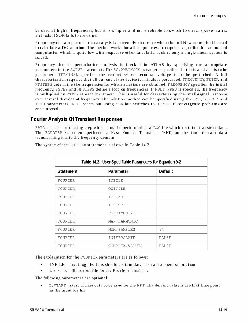
Numerical Techniques
be used at higher frequencies, but it is simpler and more reliable to switch to direct sparse matrixmethods if SOR fails to converge.
Frequency domain perturbation analysis is extremely attractive when the full Newton method is usedto calculate a DC solution. The method works for all frequencies. It requires a predictable amount ofcomputation which is quite low with respect to other calculations, since only a single linear system issolved.
Frequency domain perturbation analysis is invoked in ATLAS by specifying the appropriateparameters in the SOLVE statement. The AC.ANALYSIS parameter specifies that this analysis is to beperformed. TERMINAL specifies the contact whose terminal voltage is to be perturbed. A fullcharacterization requires that all but one of the device terminals is perturbed. FREQUENCY, FSTEP, andNFSTEPS determine the frequencies for which solutions are obtained. FREQUENCY specifies the initialfrequency. FSTEP and NFSTEPS define a loop on frequencies. If MULT.FREQ is specified, the frequencyis multiplied by FSTEP at each increment. This is useful for characterizing the small-signal responseover several decades of frequency. The solution method can be specified using the SOR, DIRECT, andAUTO parameters. AUTO starts out using SOR but switches to DIRECT if convergence problems areencountered.
Fourier Analysis Of Transient ResponsesFATR is a post-processing step which must be performed on a LOG file which contains transient data.The FOURIER statement performs a Fast Fourier Transform (FFT) on the time domain datatransforming it into the frequency domain.
The syntax of the FOURIER statement is shown in Table 14.2.
The explanation for the FOURIER parameters are as follows:
• INFILE – input log file. This should contain data from a transient simulation. • OUTFILE – file output file for the Fourier transform.
The following parameters are optional:
• T.START – start of time data to be used for the FFT. The default value is the first time pointin the input log file.
Table 14.2. User-Specifiable Parameters for Equation 9-2
Statement Parameter Default
FOURIER INFILE
FOURIER OUTFILE
FOURIER T.START
FOURIER T.STOP
FOURIER FUNDAMENTAL
FOURIER MAX.HARMONIC
FOURIER NUM.SAMPLES 64
FOURIER INTERPOLATE FALSE
FOURIER COMPLEX.VALUES FALSE
SILVACO International 14-19

ATLAS User’s Manual - Volume 2
• T.STOP – end of time data to be used for the FFT. The default value is the last time point inthe input log file.
• FUNDAMENTAL – fundamental frequency. If this is not specified, then the fundamentalfrequency is set to 1/(T.STOP - T.START). If the fundamental frequency is specified thenT.STOP is set to T.START + 1/FUNDAMENTAL.
• MAX.HARMONIC – maximum harmonic frequency that the FFT should calculate. This willautomatically calculate the correct number of samples (NUM.SAMPLES) required to generatethis frequency. FUNDAMENTAL must be specified when MAX.HARMONIC is used.
• NUM.SAMPLES – number of samples. This should be an integer power of 2, i.e. 2^n, where nis a positive integer. The default value is 64 unless the MAX.HARMONIC parameter isspecified. In this case, the number of samples is set to the nearest integer power of 2 whichwill generate this frequency.
• INTERPOLATE – performs linear interpolation on input data with non-uniform timesteps.This interpolates the data on to uniform timesteps. Interpolation of data can introduceaddition (inaccurate) harmonic values into the FFT, which would not occur if uniform timeis taken. INTERPOLATE must be used if the log file contains non-uniform time steps.
• COMPLEX.VALUES – prints the real and imaginary components to file, as well as themagnitude and phase.
Note: FFT works best with uniform time steps, therefore DT.MIN and DT.MAX on the METHODstatement should be set to the same value. The time step should be set to: time step = 1/(number of samples * fundamental frequency).
The FFT can then calculate harmonic frequencies up to:
(number of samples/2 - 1)*fundamental frequency.
Small-signal data at high frequencies can be obtained by calculating the terminal current responses toterminal voltage perturbations. The currents and voltages should then Fourier analyzed. Their ratioat each frequency provides admittance data for that frequency. The voltage perturbations are normallyselected to have an analytic form with a known Fourier transform. Care must be taken to self-consistently account for geometric capacitances when step function voltage perturbations are used.The advantages of this technique are that it can be used whenever transient calculations are possible,and each transient solution gives information over a broad range of frequencies. The maindisadvantage is that transients become very long when low frequency effects are investigated.
Overall Recommendations 1. Use frequency-domain perturbation analysis when it is available. The method works for
arbitrary frequencies and does not require transient calculations.
2. Use Fourier analysis of transient responses for high frequencies when FPDA is not availablebut transient calculations are possible.
14-20 SILVACO International
Numerical Techniques
Differences Between 2D and 3D NumericsWith respect to numerical techniques there are several differences between 2D and 3D simulations.
First, with respect to the nonlinear iteration strategies, all three strategies, NEWTON, GUMMEL andBLOCK are supported in 2D simulation, whereas, only NEWTON and GUMMEL are supported for 3Dsimulations. Implementation of the BLOCK strategy is expected in a future release.
Second, solution of the linear subproblem is handled differently for 2D and 3D simulations. Aspreviously noted the computational burden of solving the linear subproblem increases with the size ofthe solution domain. For smaller problems direct methods are quicker while for larger problemsiterative methods are preferred. It turns out that the point at which the iterative methods become lessburdensome roughly coincides with the transition between 2D and 3D domains. As such the defaultmethod for 2D simulations is a direct solver. For 3D simulations, the default method is an iterativesolver. By default ILUCGS is applied to 3D simulations. ILUCGS is an acronym for incomplete lowerupper decomposition conjugate gradient squared. Two alternative iterative solvers are also availablefor 3D simulations. BICGST (BICGST on the METHOD statement) is an acronym for biconjugate gradientsquared stabilized. GMRES (GMRES on the METHOD statement) is an acronym for generalized minimumresidual. Direct methods can be used for 3D simulation by specifying DIRECT on the METHODstatement. Practical experience shows that for 3D simulations either of the iterative methods arefaster than the direct method. However, in some cases the accuracy produced by the iterative methodscan prevent convergence in the nonlinear outer loop. For 2D simulations only direct methods aresupported.
The DC curve tracer algorithm and small signal AC analysis are also not currently supported for 3Dsimulations.
SILVACO International 14-21

ATLAS User’s Manual - Volume 2
[This page intentionally left blank]
14-22 SILVACO International

Chapter 15:Statements
entr lowercase
s
types
Overview
Input LanguageThis chapter contains a complete description (in alphabetical order) of every statement and parameter used by any ofthe ATLAS products, except for MIXEDMODE. (MIXEDMODE specific parameters are documented in theMIXEDMODE Chapter). The following documentation is provided for each statement:
• The statement name
• The product for which the statement is applicable
• The syntax of the statement
• A list of all statement parameters, their type, default value, and units
• A description of each parameter
• An example of the correct usage of each statement
Note: An error message will be generated if you attempt to specify a statement for a simulator whichyou have not purchased. For example, the BEAM statement may only be used if you have purchasedLUMINOUS or LUMINOUS3D.
Syntax RulesIn this manual, we refer to statements, and parameters. An input deck line is referred to as a statement (or statemline). Since statements and parameters are not case sensitive, they may be entered using either uppercase oletters.
A statement is specified in the general format
<STATEMENT> <PARAMETER>=<VALUE>
where STATEMENT is the statement name, PARAMETER is the parameter name, and VALUE is the parameter value.The space character is used to separate the parameters in a statement.
The words and numbers which follow a statement are parameters of that statement. A word is an alphanumeric stringwhich is terminated either by a space or by a carriage return. A number is a numeric or alphanumeric string which i
terminated either by a space or by a carriage return. Numerical values may range from 10-38 to 1038. A number maycontain the symbols + (positive), - (negative), and/or E (decimal notation). For example:
+10 -1.234E5 .003 -.12E+10
Four types of parameters are used by the ATLAS products real, integer, logical, and character. These parameter are explained in Table 15-1.
SILVACO International 15-1
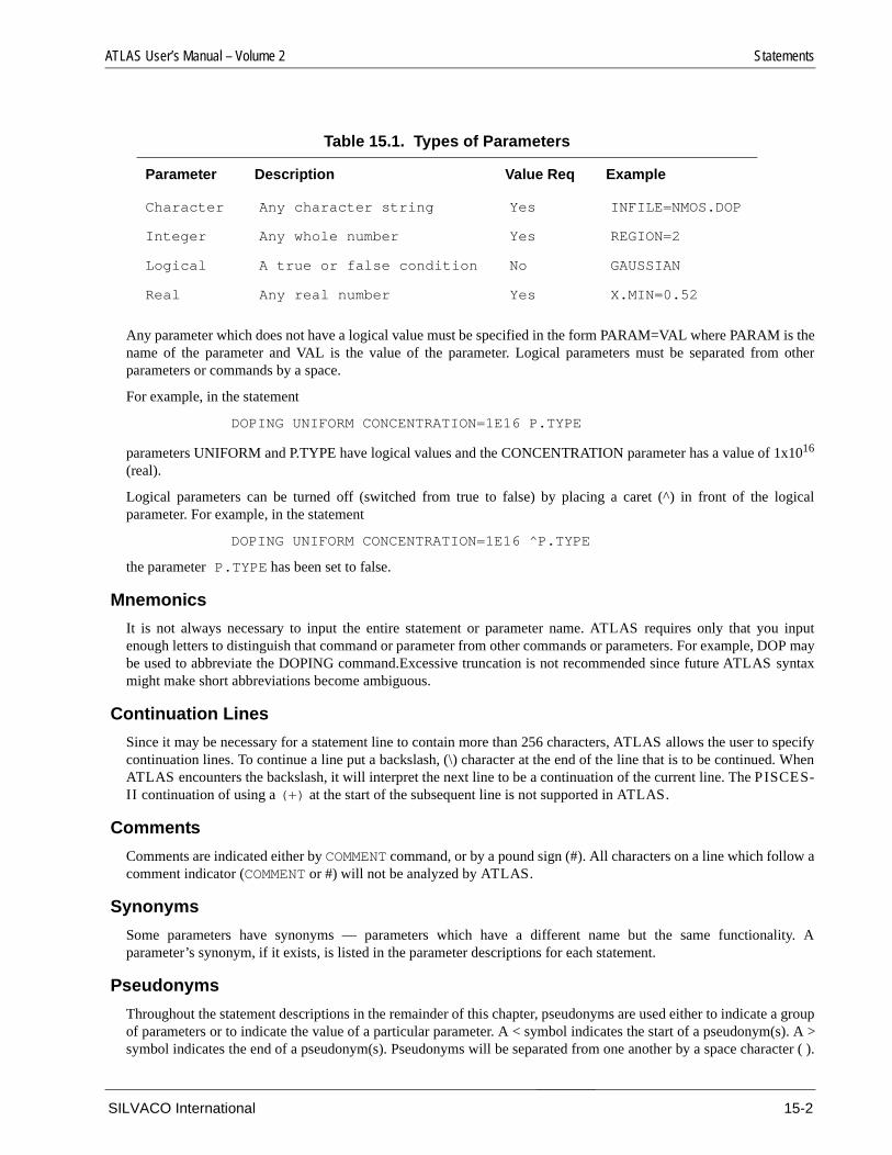
ATLAS User’s Manual – Volume 2 Statements
ality. A
e a group(s). A >
aracter ( ).
Any parameter which does not have a logical value must be specified in the form PARAM=VAL where PARAM is thename of the parameter and VAL is the value of the parameter. Logical parameters must be separated from otherparameters or commands by a space.
For example, in the statement
DOPING UNIFORM CONCENTRATION=1E16 P.TYPE
parameters UNIFORM and P.TYPE have logical values and the CONCENTRATION parameter has a value of 1x10¹⁶
(real).
Logical parameters can be turned off (switched from true to false) by placing a caret (^) in front of the logicalparameter. For example, in the statement
DOPING UNIFORM CONCENTRATION=1E16 ^P.TYPE
the parameter P.TYPE has been set to false.
Mnemonics
It is not always necessary to input the entire statement or parameter name. ATLAS requires only that you inputenough letters to distinguish that command or parameter from other commands or parameters. For example, DOP maybe used to abbreviate the DOPING command.Excessive truncation is not recommended since future ATLAS syntaxmight make short abbreviations become ambiguous.
Continuation Lines
Since it may be necessary for a statement line to contain more than 256 characters, ATLAS allows the user to specifycontinuation lines. To continue a line put a backslash, (\) character at the end of the line that is to be continued. WhenATLAS encounters the backslash, it will interpret the next line to be a continuation of the current line. The PISCES-II continuation of using a (+) at the start of the subsequent line is not supported in ATLAS.
Comments
Comments are indicated either by COMMENT command, or by a pound sign (#). All characters on a line which follow acomment indicator (COMMENT or #) will not be analyzed by ATLAS.
Synonyms
Some parameters have synonyms — parameters which have a different name but the same functionparameter’s synonym, if it exists, is listed in the parameter descriptions for each statement.
Pseudonyms
Throughout the statement descriptions in the remainder of this chapter, pseudonyms are used either to indicatof parameters or to indicate the value of a particular parameter. A < symbol indicates the start of a pseudonymsymbol indicates the end of a pseudonym(s). Pseudonyms will be separated from one another by a space ch
Table 15.1. Types of Parameters
Parameter Description Value Req Example
Character Any character string Yes INFILE=NMOS.DOP
Integer Any whole number Yes REGION=2
Logical A true or false condition No GAUSSIAN
Real Any real number Yes X.MIN=0.52
SILVACO International 15-2

Statement Statements
For example, LOC might indicate a group of location parameters and FILENAME might indicate the name of a filewhich must be specified.
Symbols
The following symbols are used in the statement descriptions throughout the rest of this chapter.
< Indicates the start of a list of pseudonyms.
> Indicates the end of a list of pseudonyms.
| Separates parameters or pseudonyms which are mutually exclusive. Only one of these parameters may be used ina statement.
[ Indicates the start of an optional command, parameter, or pseudonym.
] Indicates the end of an optional command, parameter, or pseudonym.
Expressions
ATLAS does not support arithmetic expressions in the syntax. Expressions can be evaluated and used using the SETor EXTRACT statements however.
SILVACO International 15-3

ATLAS User’s Manual – Volume 2 BEAM statement
with
BEAMBEAM — specifies an optical input signal in the form of a collimated beam of light. This statement is usedLUMINOUS or LUMINOUS3D.
Syntax
BEAM <parameters>
Parameter Type Default Units
ANGLE Real 0.0 Degrees
BACK.REFL Logical False
DEVICE Character
F.OXGENERATE Character
F.RADIATE Character
F.RADIATE3D Character
F.REFLECT Character
FRONT.REFL Logical False
ITERATION Integer 20
LENS.INDEX Real 1.0
LENS.PLANE Real 0.0 µm
LENS.RADIUS Real 0.0 µm
LENS.X Real 0.0 µm
LENS.Y Real 0.0 µm
LENS.Z Real 0.0 µm
MAX.WINDOW Real 1.0x1020 µm
METAL.REFLECT Logical False
MIN.POWER Real 0.0 µm
MIN.WINDOW Real -1.0x1020 µm
NUMBER Integer 1
NX Interger 10
NZ Integer 10
PERIODIC Logical False
PHI Real 0.0 Degrees
POLARIZE Real 0.0 Degrees
POWER.FILE Character
15-4 SILVACO International

BEAM Statement Statements
POWER.SCAL Real 1.0
QUANTUM.EFF Real 1.0
RAYS Integer 1
RAYTRACE Character
REFLECTS Integer 1
REL.POWER Real 1.0
THETA Real 0.0 Degrees
THINEST Real 0.0 µm
WAVELENGTH Real 0.623 µm
WAVEL.END Real 0.0 µm
WAVEL.NUM Integer 1
WAVEL.SCAL Real 1.0
WAVEL.START Real 0.0 µm
X.ORIGIN Real 0.0 µm
XMAX Real -1.0x1020 µm
XMIN Real 1.0x1020 µm
Y.ORIGIN Real 0.0 µm
Z.ORIGIN Real 0.0 µm
ZMAX Real -1.0x1020 µm
ZMIN Real 1.0x1020 µm
Parameter Type Default Units
SILVACO International 15-5

ATLAS User’s Manual – Volume 2 BEAM statement
Description
Figure 15-1: LUMINOUS Optical Source Coordinate System
ANGLE is the angle of propogation of the optical beam (see Figure 15-1 and 11-1). ANGLE=90 is verticalillumination from the top of the device.
Synonym: PHI
BACK.REFL specifies that back side reflections are to be taken into account. When BACK.REFL is specified, thearea outside the device domain is assumed to be a vacuum (ie. n = 1.0, k = 0.0)
DEVICE is used to specify the name of the device that the beam is associated with in MIXEDMODE simulation.
F.REFLECT specifies the name of a file containing a C-INTERPRETER function for specifying reflection coefficientmodels as a function of wavelength, position, and angle incidence (LUMINOUS only).
F.RADIATE specifies the name of a file containing a C-INTERPRETER function for specifying generation rate as afunction of position and optionally time. This function can be used to simulate single event upset (LUMINOUS only).
F3.RADIATE is the same as the F.RADIATE parameter but is applied in 3-D. This is typicallyused for single eventor photogeneration simulations with LUMINOUS3D.
FRONT.REFL specifies that front side reflections are to be taken into account. When FRONT.REFL is specified, thearea outside the device domain is assumed to be a vacuum (ie. n=1.0, k= 0.0).
LENS.INDEX sepcifies the index of refraction of a lenslet (LUMINOUS3D only).
LENS.PLANE sepcifies specifies the minimum y-cordinate of the lenslet sphere (LUMINOUS3D only).
LENS.RADIUS sepcifies the radius of the spere defining a lenslet (LUMINOUS3D only).
LENS.X sepcifies the x-coordinate of the center of the spere defining a lenslet (LUMINOUS3D only).
LENS.Y sepcifies the y-coordinate of the center of the spere defining a lenslet (LUMINOUS3D only).
LENS.Z sepcifies the z-coordinate of the center of the spere defining a lenslet (LUMINOUS3D only).
MAX.WINDOW specifies the maximum x-value of the illumination window relative to the coordinate system of theoptical beam (see Figure 15-1). The illumination window is always clipped to the device domain.
Synonym: XMAX
METAL.REFLECT sepcifies that all metals are to be treated as perfect reflectors (LUMINOUS3D only).
MIN.WINDOW specifies the minimum x-value of the illumination window relative to the coordinate system of theoptical beam.
Synonym: XMIN
15-6 SILVACO International

BEAM Statement Statements
. Rays
tween
m fileit
hoton
viewed
g of the
be used
ctor is
ee Fig.
ful for
tions.
ectral
NUMBER specifies the beam number (from 1 to 10). This number is used by the SOLVE statement to specify therelative intensity of different beams. You may specify beam numbers in any order that you desire.
NX specifies the number of rays traced along the source beam’s x axis for LUMINOUS3D (see fig11-3).
NZ specifies the number of rays traced along the source beam’s z axis for LUMINOUS3D (see fig11-3).
PERIODIC specifies that for ray tracing, the structure is to be treated as periodic in the x and z directionsexiting the sides of the device are wrapped around to the other side of the device (LUMINOUS3D only).
POLARIZE specifies the polarization of the optical beam at the origin. The polarization angle is the angle bethe E vector and the device plane.
POWER.SCALE specifies a scale factor. This factor is multiplied by each of the relative powers in the spectruwhen multi-spectral simulations are performed. The POWER.SCALE parameter can be used to perform unconversions.
POWER.FILE specifies the filename of a spectrum file. Spectrum file must be in the format
number of pairs
wavelength_1 power_1
wavelength_2 power_2
. . . . . .
. . . . . .
wavelength_n power_n
Note: The power file must contain at least two power/wavelengths pairs.
QUANTUM.EFF is a quantum efficiency factor which specifies the number of carrier pairs generated per pabsorbed.
RAYTRACE specifies the name of a file where the results of a ray trace are saved. The ray trace may beusing TONYPLOT3D (LUMINOUS3D only)
RAYS specifies the number of rays the user wishes to split the optical beam into. LUMINOUS will automatically splitthe beam into enough rays to resolve the geometry. Use of the number parameter will cause further splittinoptical beam (LUMINOUS only)
REFLECTS specifies the number of reflections that will be traced. When the value of the REFLECTS parameter isincreased, the total number of rays traced increases non-linearly. We recommend that this parameter judiciously. For example, a single ray incident on three material layers will produce 4 rays if REFLECTS=0 isspecified, 10 rays if REFLECTS=1 is specified, and 24 rays if REFLECTS=2 is specified.
REL.POWER specifies the relative power in the beam when mono-spectral simulations are performed. This famultiplied by the power parameters specified in the SOLVE statement to give the total optical power in the beam.
THETA specifies the angle of rotation for the source beam direction of propogation relative to the x-y plane (s11-2) (LUMINOUS3D only).
THINEST specifies the width of the thinnest ray to be traced (LUMINOUS only).
MIN.POWER specifies the minimum intensity relative to the source that a given ray will be traced. This is uselimiting the numbers of rays traced.
WAVELENGTH specifies the optical wavelength of the source beam (in the vacuum) for mono-spectral simula
WAVEL.END specifies the maximum wavelength of the source beam (in the vacuum) when multi-spsimulations are performed.
SILVACO International 15-7

ATLAS User’s Manual – Volume 2 BEAM statement
WAVEL.NUM specifies the number of wavelengths which will be used when multi-spectral simulations areperformed.Spectral illumination is selected when the WAVEL.NUM parameter is greater than 1. Once multi-spectralsimulations are selected, you must specify the POWER.FILE, WAVEL.START, and WAVEL.END parameters.
WAVEL.SCAL specifies the scale factor for the wavelengths which are used in multi-spectral simulations. Each ofthe wavelengths in the spectrum file is multiplied by this scale factor.
WAVEL.START specifies the minimum wavelength of the source beam (in the vacuum) when multi-spectralsimulations are performed.
XMAX specifies the maximum x-coordinate in the source beam coordinate system for ray tracing in LUMINOUS3D(see figure 11-3).
XMIN specifies the minimum x-coordinate in the source beam coordinate system for ray tracing in LUMINOUS3D(see figure 11-3).
X.ORIGIN specifies the x-coordinate of the optical beam origin (see Figures 15-1 and 11-1). The beam must originateoutside all device regions.
Y.ORIGIN specifies the y-coordinate of the optical beam origin (see Figures 15-1 and 11-1). The beam must originateoutside all device regions.
ZMAX specifies the maximum z-coordinate in the source beam coordinate system for ray tracing in LUMINOUS3D(see figure 11-1).
ZMIN specifies the minimum z-coordinate in the source beam coordinate system for ray tracing in LUMINOUS3D(see figure 11-1).
Z.ORIGIN specifies the z-coordinate of the optical beam origin (see Figure 11-1). The beam must originate outsideall device regions (LUMINOUS3D only).
Monochromatic Beam Example
This beam has a monochromatic spectrum with a wavelength of 0.6 µm. The beam originates at x=0.5 and y=-2.0. Ithas a 90 degree propogation angle and a beam width of 0.2 µm which is centered at the beam origin.During the raytrace calculation the rays will be terminated when the power level along the ray falls to 5% of the original power.
BEAM NUM=1 WAVELENGTH=0.6 X=0.5 Y=-2.0 ANG=90.0 MIN=-0.1 MAX=0.1 \
MIN.POWER=0.05
Multispectral Beam Example
A multispectral beam (at a 45 degree angle) which originates at x=0.0 and y=-1.0. The multi-spectral source isimported from the spectrum file "source.spc". The spectrum is discretized into our wavelengths between 0.4 µm and0.6 µm.
BEAM NUM=2 X=0.0 Y=-1.0 ANG=45.0 \
POWER.FILE=SOURCE.SPC WAVEL.START=0.4 \
WAVEL.END=0.6 WAVEL.NUM=4
LUMINOUS3D Lens Example
BEAM NUM=1 X.ORIGIN=2.5 Y.ORIGIN=-1.0 Z.ORIGIN = 2.5 ANG=90.0 WAVEL=0.6 \
NX=10 NZ=10 LENS.X=2.5 LENS.Y=-0.5 LENS.Z=2.5 \
LENS.INDEX=2.03 LENS.RADIUS=0.25 LENS.PLANE=-0.5
15-8 SILVACO International

COMMENT Statement Statements
COMMENT, #COMMENT – allows comments to be placed in an ATLAS input file. ATLAS will print and display comment lines.
Syntax
COMMENT [<string>]
# [<string>]
string is any alphabetic, numeric, or alphanumeric sequence of characters.
Synonyms: #
Example
COMMENT ATLAS is a copyright of Silvaco International
# ATLAS is a copyright of Silvaco International
Note: The $ was allowed as a comment character in previous versions of ATLAS. This should beavoided and replaced by the # or COMMENT statement.
15-9 SILVACO International

ATLAS User’s Manual – Volume 2 Contact Statement
CONTACTCONTACT — specifies the physical attributes of an electrode.
Note: If the CONTACT statement is not used for a given electrode, the electrode is assumed to becharge-neutral (ohmic).
Syntax CONTACT NUMBER=<n>|NAME=<ename>|ALL [<wfp>] [<bc>] [<lcr>] [<link>]
Parameter Type Default Units
ALL Logical False
ALPHA Real 0 cm
ALUMINUM Logical False
BARRIER Logical False
CAPACITANCE Real 0 F/µm
COMMOM Character
CON.RESIST Real 0 Ω·cm2
CURRENT Logical False
DEVICE Character
E.TUNNEL Logical False
ELE.CAP Integer
F.ETUNNEL Character
FACTOR Real 0
FLOATING Logical False
FG.CAP Real 0.0 F/µm
INDUCTANCE Real 0 H· µm
ME.TUNNEL Real 1.0
MO.DISILICIDE Logical False
MOLYBDENUM Logical False
MULT Logical False
NAME Character
NEUTRAL Logical True
N.POLYSILICON Logical False
15-10 SILVACO International

CONTACT Statement Statements
Description
NAME specifies the name of a previously defined electrode. See ELECTRODE statement.
NUMBER specifies the contact number to be defined. It must be the number of a previously defined electrode. It isrecommended that electrode names be used rather than numbers.
ALL defines the same properties for all electrodes.
DEVICE specifies which device the CONTACT statement applies to in MIXEDMODE.
wfp is one of the work function parameters described below. It is permitted to either specify the name of a material ora work function value (WORKFUN parameter).
bc is one or more of the boundary condition parameters .
lcr is one or more of the external parasitic element parameters .
link is one or more of a set of parameters that allow the user to associate two or more electrodes electrically.
Workfunction Parameters
ALUMINUM specifies aluminum as the contact material for the electrode. This sets the workfunction to 4.10V. Notethat this parameter should not be set if an ohmic contact is required.
MOLYBDENUM specifies molybdenum as the contact material for the electrode. This sets the work function of theelectrode to 4.53V.
MO.DISILICIDE specifies molybdenum disilicide as the contact material for the electrode. This sets the workfunction of the electrode to 4.80V.
NEUTRAL specifies that the electrode is ohmic. This is the deafult characteristic of an electrode.
N.POLYSILICON specifies n+ doped polysilicon as the contact material for the electrode. This sets the workfunction to 4.17V.
P.POLYSILICON specifies p+ polysilicon as the contact material for the electrode. This sets the work function to4.17V + Eg(Si).
TU.DISILICIDE specifies tungsten disilicide as the contact material for the electrode. This sets the work function to4.80V.
NUMBER Integer
P.POLYSILICON Logical False
RESISTANCE Real 0 Ω.µm
SHORT Logical False
SURF.REC Logical False
TU.DISILICIDE Logical False
TUNGSTEN Logical False
VSURFN Real see descrip-tion
cm/s
VSURFP Real see descrip-tion
cm/s
WORKFUN Real 0 V
Parameter Type Default Units
SILVACO International 15-11

ATLAS User’s Manual – Volume 2 Contact Statement
TUNGSTEN specifies tungsten as the contact material for the electrode. This sets the work function to 4.63V.
WORKFUN specifies the work function of the electrode in V. This parameter must be specified in the formWORKFUN=n where n is a real number. This specification is absolute workfunction and not workfunction difference tothe semiconductor.
Note: If no WORKFUN or material type parameter is specified the electrode is assumed to be an ohmiccontact
Boundary Conditions
CURRENT specifies current boundary conditions. If specified, CAPACITANCE, CON.RESIST, INDUCTANCEor RESISTANCE may not be specified.
FLOATING specifies a charge boundary condition. This parameter is used to specify the floating gate in EPROMdevices. This parameter can only be used for insulated contacts. If specified, CAPACITANCE, CON.RESIST,INDUCTANCE or RESISTANCE may not be specified, but special syntax exists for adding capacitances to afloating contact. See EL<n>.CAP and FG<n>.CAP
Synonym: CHARGE
ALPHA specifies the linear, dipole lowering coefficient. This parameter has no effect unless the BARRIER parameterhas been specified.
BARRIER turns on the barrier lowering mechanism for Schottky contacts.
E.TUNNEL specifies that the Schottky tunnelling model for electrons will be used. E.TUNNEL will also enable theSURF.REC boundary condition which models the thermionic emission in a Schottky contact.
F.ETUNNEL specifies the name of a file containing a C-INTERPRETER function that specifies electron tunnelling ata Schottky contact.
ME.TUNNEL specifies the relative effective mass for use in the electron tunneling mode (see E.TUNNEL).
SURF.REC specifies that finite surface recombination velocities are used at the respective contact. This parametermust be specified in the form SURF.REC [VSURFN=<n>] [VSURFP=<p>], where n and p are real numbers.
VSURFN specifies the actual surface recombination velocities for electrons (Vsn). If this parameter is not specified,its default value is calculated by Equation 15-1.
15-1
where ARICHN is the effective Richardson constant for electrons. This constant accounts for quantum mechanicalreflections and tunneling.
VSURFP specifies the actual surface recombination velocities for holes (Vsp). If this parameter is not specified, its
default value is calculated by Equation 15-2.
15-2
where ARICHP is the effective Richardson constants for holes. This constant accounts for quantum mechanicalreflections and tunneling.
VsnARICHNT
2
qNC--------------------------=
VspARICHPT
2
qNV--------------------------=
15-12 SILVACO International

CONTACT Statement Statements
n theias on
torode
iles and
er in the accountr extra
lectrode
es finiteition in
Contact Parasitics
Note: There are restrictions on the allowed numerical methods and types of analysis possible when anyform of parasitic element is attached to a contact. See the Getting Started section for details.
RESISTANCE specifies a lumped resistance value. You may not specify both RESISTANCE and CON.RESIST.
INDUCTANCE specifies an external inductance which is related to the specified electrode. A synonym is L
CAPACITANCE specifies a lumped capacitance value to be attached to the contact.
CON.RESIST specifies a distributed contact resistance. You cannot specify both CON.RESIST and RESIST.
Electrode Linking Parameters
These parameters allow one electrode to be biased as a function of another electrode. This allows separate regions ofthe same physical contact to be linked together. For example, in the statement:
CONTACT NAME=MYDRAIN COMMON=DRAIN FACTOR=4.6
Electrode ‘mydrain’ is linked to the electrode ‘drain’. The bias on ‘mydrain’ will always be equal to the bias odrain plus 4.6. If the optional MULT parameter had been specified, the bias on my drain would be equal to the bthe drain multiplied by 4.6.
COMMON specifies the electrode name to which the contact refered to by NAME is linked. Although the electrodesare linked separate currents will be saved for both electrodes unless SHORT is also specified. The electrode refered in NAME should not appear on any SOLVE statments since it’s bias is now determined as a function of the electrefered to by COMMON.
SHORT specifies that the electrode referred to by NAME is shorted to the electrode specified by the COMMONparameter. This implies that the two electrodes will be treated as one and only one value will be written to log fin the run time output.
FACTOR specifies the constant offset voltage (or current) between the electrodes refered by by NAME and COMMON.By default, FACTOR is added the defined voltage.
MULT specifies that FACTOR is a multiplier.
Floating Gate Capacitance Parameters
In same cases it is desirable to simulate floating gate structures, in 2D, which have control gates that are longunsimulated dimension than the floating gate. In these cases the user can specify the following parameters tofor addition capacitance between the floating gate and the control gate and other electrodes.Up to foucapacitances are allowed so in the following <n> is an integer number between 1 and 4.
EL<n>.CAP specifies the name of the electrode to which the extra capacitance is linked.
FG<n>.CAP specifies the additional capacitance per unit length to be added between the floating gate and especified in EL<n>.CAP.
Schottky Barrier and Surface Recombination Example
This example defines all electrodes except number 2 (aluminum) to be neutral. Electrode number 2 also includsurface recombination velocities and barrier lowering. A definition in the second statement overrides that definthe first statement.
CONTACT ALL NEUTRAL
CONTACT NUMBER=2 ALUMINUM SURF.REC BARRIER
SILVACO International 15-13

ATLAS User’s Manual – Volume 2 Contact Statement
added
Parasitic Resistance Example
This example attaches a lumped resistor with a value of 105Ωµm to the substrate. A distributed contact resistance of
10-6Ω·cm2 is included on the drain.
CONTACT NAME=substrate RESISTANCE=1E5
CONTACT NAME=drain CON.RESIST=1E-6
Floating Gate Example
This syntax defines a floating contact with a workfunction equal to 4.17eV. An extra 1fF/um capacitance isbetween this electrode and the electrode named ‘cgate’
CONTACT NAME=fgate FLOATING N.POLY EL1.CAP=cgate FG1.CAP=1e-15
Note: The command, MODELS PRINT, can be used to echo the back contact workfunction andparasitic elements settings to the run-time output
15-14 SILVACO International

CURVETRACE Statement Statements
of theres
CURVETRACE CURVETRACE – sets the parameters for the automatic curve tracing routine.
Syntax
CURVETRACE <params>
Note: The curvetracer functionality of ATLAS creates several temporary files in the local directory inwhich it is run. Two simultaneous ATLAS runs using curvetrace in the same directory will interfere witheach other.
Description
ANGLE1, ANGLE2 and ANGLE3 are critical angles (in degrees) affecting the smoothness and step size trace. If the difference in slopes of the last two solution points is less than ANGLE1, the step size will be increased fothe next projected solution. If the difference lies between ANGLE1 and ANGLE2, the step size remains the same. If thdifference is greater than ANGLE2, the step size is reduced. ANGLE3 is the maximum difference allowed, unlesoverridden by the MINDL parameter. ANGLE2 should always be greater than ANGLE1 and less than ANGLE3.
BEG.VAL is the value of the voltage at the starting point of the curve trace for the controlling electrode.
CONTR.ELEC is the number of the electrode that is designated as a control electrode.
Parameter Type Default Units
ANGLE1 Real 5
ANGLE2 Real 10
ANGLE3 Real 15
BEG.VAL Real 0.0 V
CONTR.ELEC Integer
CONTR.NAME Character
CURR.CONT Logical
END.VAL Real
MINCUR Real
MINDL Real 0.1
NEXTST.RATIO Real 2.0
STEP.CONT Logical
STEP.INIT Real 0.1 V
STEPS Real 0.1
TURNINGPOINT Logical False
VOLT.CONT Logical False
SILVACO International 15-15

ATLAS User’s Manual – Volume 2 CURVETRACE Statement
CONTR.NAME is the name of the control electrode.
CURR.CONT denotes that a maximum current on the control electrode, specified by END.VAL is used as the upperbound on the trace.
END.VAL is used to stop tracing if the voltage or current of control electrode equals or exceeds END.VAL.
NEXTST.RATIO specifies which factor to use to increase the voltage step on the smooth parts of the I-V curve.
MINCUR may be used to set a small current value in order to switch from internal control electrode bias ramping toexternal ramping with load resistor. This parameter is recommended for small current breakdown simulation.
MINDL is the minimum normalized step size allowed in the trace. Usually the user does not need to adjust thisparameter. Increasing MINDL will reduce the smoothness of the trace by overriding the angle criteria, resulting inmore aggressive projection and fewer simulation points. Reducing MINDL will enhance the smoothness and increasethe number of points in the trace.
STEPS is the number of operational points on a trace if STEP.CONT was specified.
STEP.CONT specifies that the trace will proceed for a certain number of simulation points.
STEP.INIT specifies initial voltage step size.
Note: To set a sweep of increasingly negative voltage in CURVETRACE it is only necessary to setSTEP.INIT to be negative. Since all parameters are multiplier of STEP.INIT the whole voltagesweep will be negative.
TURNINGPOINT specifies that binary output solution files will be saved whenever the slope of the IV curvechanges sign; i.e. there is a turning point. The name of the output file is "soln.num", where num is the number of thecurrent solution.
VOLT.CONT denotes that a maximum voltage on the control electrode, specified by END.VAL is used as the upperbound on the trace.
Diode Breakdown Example
To trace a diode breakdown curve using current value as a termination criteria, the following statement may be used:
CURVETRACE CURR.CONT END.VAL=0.01 CONTR.NAME=anode \
MINCUR=5E-12 NEXTST.RATIO=1.1 STEP.INIT=0.1
SOLVE CURVETRACE
15-16 SILVACO International

DEFECT Statement Statements
thin-film
DEFECTDEFECT — activates the band gap defect model and sets the parameter values. This model can be used whentransistor simulations are performed using the TFT product.
Syntax
DEFECTS [<parameters>]
Parameter Type Default Units
AFILE Character
CONTINUOUS Logical True
DEVICE Character
DFILE Characater
EGA Real 0.4 eV
EGD Real 0.4 eV
F.TFTACC Character
F.TFTDON Character
NGA Real 5.0x1017 cm-3
NGD Real 1.5x1018 cm-3
NTA Real 1.12x1021 cm-3/eV
NTD Real 4.0x1020 cm-3/eV
NUMBER Real All
NUMA Real 12
NUMD Real 12
SIGGAE Real 1.0x10⁻¹⁶ cm2
SIGGAH Real 1.0x10⁻¹⁴ cm2
SIGGDE Real 1.0x10⁻¹⁴ cm2
SIGGDH Real 1.0x10⁻¹⁶ cm2
SIGTAE Real 1.0x10⁻¹⁶ cm2
SIGTAH Real 1.0x10⁻¹⁴ cm2
SIGTDE Real 1.0x10⁻¹⁴ cm2
SOGTDH Real 1.0x10⁻¹⁶ cm2
WGA Real 0.1 eV
SILVACO International 15-17

ATLAS User’s Manual – Volume 2 DEFECT Statement
onential
stored.
d. This
nergy is
nergy is
r
r
ceptor
states.
Description
The DEFECTS statement is used to describe the density of defect states in the band gap. Up to four distributions can bespecified — two for donor-like states and two for acceptor-like states. Each type of state may contain one exp(tail) distribution and one Gaussian distribution.
AFILE specifies the file name in which the acceptor state density distribution as a function of energy will be This file can be examined using TONYPLOT.
CONTINUOUS specifies that the continuous defect integral model will be used.
DEVICE specifies which device the statement applies in mixed mode simulation
DFILE specifies the file name in which the donor state density distribution as a function of energy will be storefile can be examined using TONYPLOT.
EGA specifies the energy that corresponds to the Gaussian distribution peak for acceptor-like states. This emeasured from the conduction band edge.
EGD specifies the energy that corresponds to the Gaussian distribution peak for donor-like states. This emeasured from the valence band edge.
F.TFTACC specifies the name of a file containing a C-INTERPRETER function describing the distribution of acceptostate densities as a function of energy.
F.TFTDON specifies the name of a file containing a C-INTERPRETER function describing the distribution of donostate densities as a function of energy.
NGA specifies the total density of acceptor-like states in a Gaussian distribution.
NGD specifies the total density of donor-like states in a Gaussian distribution.
NTA specifies the density of acceptor-like states in the tail distribution at the conduction band edge.
NTD specifies the density of donor-like states in the tail distribution at the valence band edge.
NUMBER or REGION specifies the region index to which the DEFECT statement applies.
NUMA specifies the number of discrete levels that will be used to simulate the continuous distribution of acstates.
NUMD specifies the number of discrete levels that will be used to simulate the continuous distribution of donor
SIGGAE specifies the capture cross-section for electrons in a Gaussian distribution of acceptor-like states.
SIGGAH specifies the capture cross-section for holes in a Gaussian distribution of acceptor-like states.
SIGGDE specifies the capture cross-section for electrons in a Gaussian distribution of donor-like states.
SIGGDH specifies the capture cross-section for holes in a Gaussian distribution of donor-like states.
SIGTAE specifies the capture cross-section for electrons in a tail distribution of acceptor-like states.
SIGTAH specifies the capture cross-section for holes in a tail distribution of acceptor-like states.
SIGTDE specifies the capture cross-section for electrons in a tail distribution of donor-like states.
SIGTDH specifies the capture cross-section for holes in a tail distribution of donor-like states.
WGA specifies the characteristic decay energy for a Gaussian distribution of acceptor-like states.
WGD Real 0.1 eV
WTA Real 0.025 eV
WTD Real 0.05 ev
Parameter Type Default Units
15-18 SILVACO International

DEFECT Statement Statements
WGD specifies the characteristic decay energy for a Gaussian distribution of donor-like states.
WTA specifies the characteristic decay energy for the tail distribution of acceptor-like states.
WTD specifies the characteristic decay energy for the tail distribution of donor-like states.
TFT Example
The following statement lines specify distributed defect states which would typically be used for polysilicon.
DEFECTS NTA=1.E21 NTD=1.E21 WTA=0.033 WTD=0.049 \
NGA=1.5E15 NGD=1.5E15 EGA=0.62 EGD=0.78 \
WGA=0.15 WGD=0.15 SIGTAE=1.E-17 \
SIGTAH=1.E-15 SIGTDE=1.E-15 SIGTDH=1.E-17 \
SIGGAE=2.E-16 SIGGAH=2.E-15 SIGGDE=2.E-15 \
SIGGDH=2.E-16
SILVACO International 15-19

ATLAS User’s Manual – Volume 2 DEGRADATION Statement
e
e
r
rappingshift in
DEGRADATIONDEGRADATION – specifies parameters for MOS device degradation modeling.
Syntax
DEGRADATION <params>
Description
NTA specifies the uniform acceptor-like trap density on the interface.
NTD specifies the uniform donor-like trap density on the interface.
SIGMAE specifies the acceptor-like trap capture cross section.
SIGMAH specifies the donor-like trap capture cross section.
F.NTA specifies the file name for a C-INTERPRETER function that specifies arbitrary density distribution of thacceptor-like traps on the interface.
F.NTD specifies the file name for a C-INTERPRETER function that specifies arbitrary density distribution of thdonor-like traps on the interface.
F.SIGMAE specifies the name of a file containing a C-INTERPRETER function specifying the distribution of acceptotrap cross-sections.
F.SIGMAH specifies the name of a file containing a C-INTERPRETER function specifying the distribution of donortrap cross-sections.
MOS Interface State Example
DEGRADATION NTA=1.E-12 SIGMAE=5.E-18
This syntax defines a density of acceptor states uniformly distributed along the silicon-oxide interface. The tcross section is also defined. Traps will be filled by gate current in transient mode simulations leading to a device parameters.
Parameter Type Default Units
F.NTA Char
F.NTD Char
F.NTD Char
F.SIGMAE Char
F.SIGMAH Char
NTA Real 1.0x1011 cm-2
NTD Real 1.0x1010 cm-2
SIGMAE Real 1.0x1017 cm-2
SIGMAH Real 1.0x1017 cm-2
15-20 SILVACO International
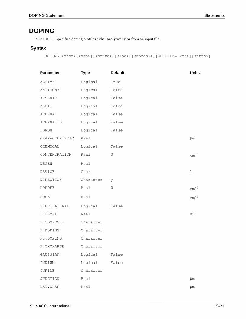
DOPING Statement Statements
DOPINGDOPING — specifies doping profiles either analytically or from an input file.
Syntax
DOPING <prof>[<psp>][<bound>][<loc>][<sprea>>][OUTFILE= <fn>][<trps>]
Parameter Type Default Units
ACTIVE Logical True
ANTIMONY Logical False
ARSENIC Logical False
ASCII Logical False
ATHENA Logical False
ATHENA.1D Logical False
BORON Logical False
CHARACTERISTIC Real µm
CHEMICAL Logical False
CONCENTRATION Real 0 cm-3
DEGEN Real
DEVICE Char 1
DIRECTION Character y
DOPOFF Real 0 cm-3
DOSE Real cm-2
ERFC.LATERAL Logical False
E.LEVEL Real eV
F.COMPOSIT Character
F.DOPING Character
F3.DOPING Character
F.OXCHARGE Character
GAUSSIAN Logical False
INDIUM Logical False
INFILE Character
JUNCTION Real µm
LAT.CHAR Real µm
SILVACO International 15-21

ATLAS User’s Manual – Volume 2 DOPING Statement
MASTER Logical False
N.TYPE Logical False
NET Logical False
OUTFILE Character
PHOSPORUS Logical False
P.TYPE Logical False
RATIO.LATERAL Real 0.7
REGION Real
RESISTI Real
OX.CHARGE Logical False
REGION Integer All
SIGN Real cm2
SIGP Real cm2
SLICE.LAT Real µm
START Real 0
SUPREM3 Logical False
TAUN Real
TAUP Real
TRAP Logical False
UNIFORM Logical False
X.COMP Logical False
X.LEFT Real left of structure µm
X.MAX Real µm
X.MIN Real µm
X.RIGHT Real right of structure µm
Y.BOTTOM Real bottom of structure µm
Y.COMP Logical False
Y.MAX Real µm
Y.MIN Real µm
Y.TOP Real top of structure
Z.BACK Real
Parameter Type Default Units
15-22 SILVACO International

DOPING Statement Statements
Description
The DOPING statement is used to define doping profiles in the device structure. Typically a sequence of DOPINGstatements is given each building on the others.
OUTFILE specifies the name of an output file for use with REGRID. The first DOPING statement should use thisparameter to specify a filename. All doping information from the first DOPING statement and all subsequent DOPINGstatements in the input file are saved to this file. The REGRID statement can read this file and interpolate doping onthe new grid.
Note: The file from OUTFILE cannot be used in TONPLOT or in the MESH statement.The SAVEcommand should be used after all of the DOPING commands required to save a file for plotting thedoping profile.
Analytical Profile Types
These parameters specify how ATLAS will generate a doping profile from analytical functions.
GAUSSIAN specifies the use of a gaussian analytical function to generate the doping profile. If GAUSSIAN isspecified, the following parameters must also be specified:
Polarity parameters N.TYPE or P.TYPE
One of the following groups of profile specifications:
Group 1:CONCENTRATION and JUNCTION
Group 2:DOSE and CHARACTERISTIC
Group 3:CONCENTRATION and CHARACTERISTIC
UNIFORM specifies the use of uniform (constant) analytical functions to generate the doping profile. If Uniform isspecified, the N.TYPE, P.TYPE, and CONCENTRATION parameters must be specified. Doping is introduced intoa box defined by the boundary parameters (see page 15-25). The box by default includes the entire region.
F.DOPING specifies the name of a file containing a C-INTERPRETER function specifying the spatial distribution ofdopants.
F3.DOPING specifies the name of a file containing a C-INTERPRETER function specifying the spatial distribution ofdopants for a 3D device.
Z.FRONT Real
Z.MIN Real
Z.MAX Real
ZLAT.CHAR Real
ZSLICE.LAT Real
ZRATIO.LAT Real 0.7
Parameter Type Default Units
SILVACO International 15-23

ATLAS User’s Manual – Volume 2 DOPING Statement
dentrations
the
ryasg profile
he
ch
,
Different
tration isns
File Import Profile Types
These parameters specify how ATLAS will generate a doping profile from a file. Files can be user-defined or fromprocess simulation.
INFILE specifies the name of the appropriate input file.
ASCII has two separate meanings:
• when combined with other format parameters is specifies the filetype is ASCII
• when used alone, it specifies ASCII data files containing concentration versus depth information.
In the second meaning this parameter must be written in the form ASCII INFILE=<filename>, wherefilename is the name of the ASCII input file. The data file must be in the following format:
depth concentration
depth concentration
depth concentration
...
where depth is specified in µm and concentration is specified in cm-3. An input file name, a dopant type, anboundary parameters must be specified. Positive concentrations are assumed to be n-type and negative concare assumed to be p-type unless the N.TYPE or P.TYPE parameters are used.
MASTER specifies that the INFILE is written in the Silvaco standard structure file format. This file format is default output format of ATHENA and SSUPREM3. This parameter is typically combined with the SSUPREM3,ATHENA 1D or ATHENA parameters. If neither of these are used the default is SSUPREM3.
SUPREM3 specifies the INFILE was produced by SSUPREM3 in standard structure file (SSF) format or binaor an ASCII export format. Export format is an obsolete file format. If this profile type is used, an input file name, dopant, and boundary parameters must be specified. When SSUPREM3 produces an output file, the doping profileare stored by dopant. Therefore, a dopant parameter should be specified in order to import the correct dopininto ATLAS. If a specific dopant is not specified the total donors and acceptor concentrations are loaded.
ATHENA.1D specifies that the doping file is a ATHENA 1D export file. This parameter acts in a similar way to tSSUPREM3 parameter.
ATHENA reads 2D doping information from ATHENA standard structure file (SSF) or PISCES-II format files.The PISCES-II format is an obsolete file format.. Doping information obtained from this file will be added to eapoint of the current ATLAS mesh. If points in the ATLAS mesh do not coincide with points in the ATHENA mesh,doping for ATLAS mesh points will be interpolated from ATHENA doping information. If this profile type is usedthe INFILE parameter must also be specified.
Note: The X.STRETCH function available in previous versions of ATLAS has been replaced by similarmore powerful functions in DEVEDIT. This feature should no longer be used in ATLAS.
Parameters that Specify the Dopant Type
These parameters give information about the dopant species or type to be used inthe specified profile. profile types require different profile specifications.
ACTIVE specifes that for the dopant specified the active concentration as opposed to the chemical concenadded. This is true by default. Files from ATHENA or SSUPREM3 contain both active and chemical concentratiofor each dopant.
ANTIMONY specifies that antimony dopant information be extracted from an imported file.
ARSENIC specifies that arsenic dopant information be extracted from an imported file.
15-24 SILVACO International

DOPING Statement Statements
is not
d of the
(x or
BORON specifies that boron dopant information be extracted from an imported file.
CHEMICAL specifies that the chemical concentration (as opposed to the active concentration) will be read from theimported file. This is generally not advisable.
DOPOFF subtracts a background doping value from the ATHENA or SSUPREM3 doping.
INDIUM specifies that indium dopant information be extracted from an imported file.
NET specifies that net doping information be extracted from an imported file. This is usually not advisable. It isbetter to use several DOPING statements to extract data dopant by dopant from a file.
N.TYPE, DONOR specifies an n-type or donor dopant. This parameter may be used with GAUSSIAN and UNIFORMprofile types.
P.TYPE, ACCEPTOR specifies a p-type or acceptor dopant. This parameter may be used with GAUSSIAN andUNIFORM profile types.
PHOSPHORUS specifies that phosphorus dopant information be extracted from an imported file.
TRAP specifies that the dopant concentration is to be treated as a trap state density.
OX.CHARGE specifies a fixed oxide charge profile. Oxide charge can only be placed in any insulator region. TheN.TYPE/P.TYPE parameters are not used hence a negative concentration implies a negative charge.
X.COMP specifies a profile of composition fraction x as defined in Appendix B. This profile can be usedto change the composition fraction of cations in terniary and quaterniary materials over a spatial distribution.
Y.COMP specifies a profile of composition fraction y as defined in Appendix B. This profile can be usedto change the composition fraction of anions in terniary and quaterniary materials over a spatial distribution.
RESISTI can be used to specify resistivity, which is converted to carrier concentration in silicon (i.e. this parameterreplaces the CONC parameter). This conversion uses tables of resistivity versus concentration for donors andacceptors. These tables currently make no distinction between specific changes of the same type. The Arora mobilitymodel is the basis of these tables.
Vertical Distribution Parameters
CHARACTERISTIC specifies the principal characteristic length of the implant. If this parameter is left unspecified,the principal characteristic can be computed from the values of the
• Polarity Parameters
• Boundary Parameters
• Concentration and Junction parameters
CONCENTRATION specifies the peak concentration when a Gaussian profile is used. If this parameter specified, peak concentration may be computed from the values of the polarity, boundary, DOSE, or RESISTI,CHARACTERISTIC concentrations. When a uniform profile is specified, the CONCENTRATION parameter sets thevalue of the uniform doping level. Concentrations must be positive.
DOSE specifies the total dose for a Gaussian profile.
JUNCTION specifies the location of a p-n junction within the silicon region of a Gaussian profile. When JUNCTIONis specified, the characteristic length is computed by examining the doping at a point halfway between the enconstant box and the given depth. The JUNCTION location is evaluated considering all previous DOPING statementsonly. This means that in some cases the order of DOPING statements is important.
PEAK specifies the depth location of the peak doping in a Gaussian profile.
Location Parameters
DIRECTION specifies the axis along which a one-dimensional profile is directed in a two-dimensional devicey). DIR=y will typically be used for implanted profiles.
REGION specifies the region number where doping is to be added.
SILVACO International 15-25

ATLAS User’s Manual – Volume 2 DOPING Statement
START specifies the depth in the y direction where the profile should start.
Lateral Extent Parameters
These parameters must be specified when a 1-D doping profile type is used (MASTER, GAUSSIAN, or ASCII).These boundary parameters set the doping boundaries before applying lateral spreading. This is equivalent to settingimplant mask edges.
X.MIN, X.MAX, Y.MIN, Y.MAX, Z.MIN and Z.MAX specify the x, y and z bounds of a rectangular shapedregion or box in the device. The dopant profile within this box will be constant with a density equal to the valuespecified by the CONC parameter. Outside this box the profile decreases from the peak, CONC, with distance, from thebox along the principal axes. The relationship between the concentration, outside the box, to distance will dependupon the profile type as specified by the GAUSSIAN, MASTER, ATHENA, ATLAS, and UNIFORM parameters.
X.LEFT, XMIN specifies the left boundary of a vertical 1-D profile.
X.RIGHT, X.MAX specifies the right boundary of a vertical 1-D profile.
Y.BOTTOM, Y.MAX specifies the bottom boundary of a horizontal 1-D profile.
Y.TOP, Y.MIN specifies the top boundary of a horizontal 1-D profile.
Z.BACK, Z.MIN specifies the back boundary of a z directed 1-D or 2-D profile.
Z.FRONT, Z.MAX specifies the front boundary of a z directed 1-D or 2-D profile.
Lateral Distribution Parameters
These parameters specify how a vertical 1-D profile is extended outside the box defined by the lateral extentparameters.
LAT.CHAR specifies the characteristic length of the lateral profile. If this parameter is not specified, thecharacteristic length is defined by:
CL = RL x OCL
where:
CL is the lateral characteristic length in the x direction.
RL is the value of RATIO.LATERAL.
OCL is the characteristic length of the original profile in the y direction.
ERFC.LATERAL specifies an error function used for lateral spreading. If two-dimensional spreading parameters areused in conjunction with a Gaussian profile, the lateral impurity profile may be transformed into an error function.
RATIO.LATERAL is the ratio of characteristic lengths in the x and y directions.
SLICE.LAT specifies the point at which the doping is examined to compute the characteristic length of a Gaussianprofile after JUNCTION has been specified. The default for this parameter is a point halfway between the end of theconstant box and the given depth.
ZLAT.CHAR specifies the characteristic length of the laterial profile in the z direction. See also LAT.CHAR.
ZRATIO.LATERAL is used analogously to RATIO.LATERAL but applies to lateral spreading in the z direction. Seealso LAT.CHAR.
ZSLICE.LAT is analogous to SLICE.LAT but applies to profiels in the z direction.
Trap Parameters
Note: See the TRAP statement for more information on each of these parameters
15-26 SILVACO International
DOPING Statement Statements
DEVICE specifies which device the statement applies to in MIXEDMODE simulation.
REGION specifies which region the traps apply to. If unspecified, the traps apply to all regions.
E.LEVEL sets the energy of the discrete trap level. For acceptors E.LEVEL is relative to the conduction band edge,for donors it is relative to the valence band edge.
DEGEN.FAC specifies the degeneracy factor of the trap level used to calculate the density.
SIGN speccifies the capture cross section of the trap for electrons.
SIGP specifies the capture cross section of the trap for holes.
TAUN specifies the lifetime of electrons in the trap level.
TAUP specifies the lifetime of holes in the trap level
Analytical Doping Defintion Example
This example describes a 1.0µm n-channel MOSFET using Gaussian source and drain profiles. The lateral extent ofthe source is given by X.RIGHT=2. This corresponds to the mask edge for the implant. Sub-diffusion is determined byan error function based on the RATIO.LAT and JUNCTION parameters. For both source and drain, the n+ doping isadded to the uniform p-well concentration to ensure a junction depth of 0.3µm.
DOP UNIF CONC=1E16 P.TYPE
DOP GAUSS CONC=9E19 N.TYPE X.RIGHT=2 JUNC=0.3 RATIO.LAT=0.6 ERFC.LAT
DOP GAUSS CONC=9E19 N.TYPE X.LEFT=3 JUNC=0.3 RATIO.LAT=0.6 ERFC.LAT
1D ATHENA or SSUPREM3 Interface Example
This example reads a 1D ATHENA bipolar profile and adds it to a uniform substrate concentration. The base andemitter doping are loaded from the same file by specifying the impurity required for each area (boron in the base andarsenic in the emitter).
The DOPOFF parameter is used to subtract the substrate arsenic dopant out of the 1-D profile that is loaded since thisdopant was already specified in the substrate doping line.
Versions of SSUPREM3 later than 5.0 use standard structure files as default when saving data. These can be loadedin ATLAS with the syntax below by replacing ATHENA.1D with SSUPREM3.
# SUBSTRATE
DOP REGION=1 UNIF CONC=1E16 N.TYPE
# BASE
DOP REGION=1 MASTER ATHENA.1D BORON RATIO.LAT=0.7 INF=bipolar.exp
# EMITTER
DOP REGION=1 MASTER ATHENA.1D ARSENIC RATIO.LAT=0.6 \
INF=bipolar.exp X.LEFT=12.0 X.RIGHT=13.0 DOPOFF=1e16
Athena Doping Interface Example
This example demonstrates how to use an SSF format ATHENA file to interpolate doping onto a ATLAS grid andsave the doping information for subsequent regrid operations.This is an alternative the prefered Athena/Atlasinterface which is documented in the Getting Started Chapter.
DOPING ATHENA MASTER INFILE=NMOS.DOP OUTFILE=NMOS.DOP
REGRID DOPING ABS LOG RATIO=4 OUTFILE=NMESH1.STR DOPFILE=NMOS.DOP
SILVACO International 15-27

ATLAS User’s Manual – Volume 2 DOPING Statement
3D Doping Defintion Example
The following example illustrates the formation of a Gaussian highly doped n-type area in a three-dimensionalstructure.
DOPING GAUSS N.TYPE CONC=1e20 PEAK=0.0 CHAR=0.2 X.LEFT=0.5 \
X.RIGHT=1.0 Z.LEFT=0.5 Z.RIGHT=1.0
15-28 SILVACO International

ELECTRODE Statement Statements
d opticalsuch as
ELECTRODEELECTRODE — specifies the locations and names of electrodes in a previously defined mesh.
Syntax
ELECTRODE NAME=<en> [NUMBER=<n>] [SUBSTRATE] <pos> <reg>
Description
MATERIAL specifies a material for the electrode (see Table B-1). This material will be displayed in TONYPLOT. Theelectrode material can also be used to define the electrode thermal characteristics (thermal conductivity) ancharacteristics (complex index of refraction). Setting the material here does not apply any electrical property workfunction to the terminal. All electrical properties of electrodes are set on the CONTACT statement.
Parameter Type Default Units
BOTTOM Logical False
IX.HIGH Integer right side of structure
IX.LOW Integer left side of structure
IY.HIGH Integer IY.LOW
IY.LOW Integer top of structure
IZ.HIGH Real
IZ.LOW Real
LEFT Logical False
LENGTH Real length of structure µm
MATERIAL Character Contact
NAME Character
NUMBER Integer defined #(electrodes)+ 1
RIGHT Logical False
SUBSTRATE Logical False
TOP Logical False
X.MAX Real right side of structure µm
X.MIN Real left side of structure µm
Y.MAX Real Y.MIN µm
Y.MIN Real top of the structure µm
Z.MIN Real µm
Z.MAX Real µm
SILVACO International 15-29

ATLAS User’s Manual – Volume 2 ELECTRODE Statement
NAME specifies an electrode name. Since other parts of the program use standard electrode names it is suggested thatthese names be used.The list of allowed names by other syntax is: gate, gg, drain, dd, source, bulk, substrate,emitter, ee, collector, cc, base, bb, anode, cathode, fgate, cgate, ngate, pgate, well, nwell, pwell, channel, andground
NUMBER specifies an electrode number from 1 to 50. Electrode numbers may be specified in any order. If NUMBERis not specified, electrodes will be automatically numbered in sequential order. This parameter cannot renumberelectrodes already defined in ATLAS or other programs.
SUBSTRATE places the specified electrode at the bottom of the device and names the electrode substrate.
pos is one of the position parameters described below.
reg is a set of the region parameters described on the next page.
Position Parameters
BOTTOM or SUBSTRATE specifies that the electrode is positioned along the bottom of the device.
LEFT specifies that the electrode starts at the left-hand edge of the device. The electrode will be positioned from leftto right along the top of the device.
RIGHT specifies that the electrode starts at the right-hand edge of the device. The electrode will be positioned fromright to left along the top of the device.
TOP specifies that the electrode is positioned along the top of the device.
Region Parameters
Device coordinates may be used to add regions to both rectangular and irregular meshes. In either case, boundariesmust be specified with the X.MAX, X.MIN, Y.MAX, and Y.MIN parameters.
LENGTH specifies the length of the electrode in the x-direction. It is not necessary to specify X.MIN, X.MAX, andLENGTH. If two of these parameters are specified, the value of the third parameter willbe calculated.
X.MAX specifies the maximum x-boundary of the electrode.
X.MIN specifies the minimum x-boundary of the electrode.
Y.MAX specifies the maximum y-boundary of the electrode.
Y.MIN specifies the minimum y-boundary of the electrode..
Z.MIN specifies the minimum z-boundary of the electrode.
Z.MAX specifies the maximum z-boundary of the electrode.
Note: If an electrode has been shortened to fit the current mesh, a warning message will be generatedby ATLAS. Electrode placement can only occur at previously defined mesh nodes.
Grid Indices
As an alternative to the region parameters above, it is permitted to use grid indices to define a region only when themesh is rectangular although these parameters are not recommended. To define a region with a rectangular mesh:
1. The X.MESH and Y.MESH statements must be used to specify grid indices.
2. The IX.HIGH, IX.LOW, IY.HIGH, and IY.LOW parameters may be used to specify x and y values.
IX.HIGH specifies the maximum x-value of the grid index.
IX.LOW specifies the minimum x-value of the grid index.
15-30 SILVACO International

ELECTRODE Statement Statements
IY.HIGH specifies the maximum y-value of the grid index
IY.LOW specifies the minimum y-value of the grid index.
Nodes which have x and y grid indices between IX.LOW and IX.HIGH and between IY.LOW and IY.HIGH aredesignated electrode nodes. Normally, horizontal planar electrodes will be used. In this case, IY.LOW equalsIY.HIGH.
IZ.HIGH specifies the maximum z-value of the grid index.
IZ.LOW pecifies the minimum z-value of the grid index.
MOS Electrode Definition Example
This example defines electrodes for a typical MOS structure.
ELEC X.MIN=0.5 LENGTH=0.25 NAME=gate
ELEC LENGTH=0.25 Y.MIN=0 LEFT NAME=source
ELEC LENGTH=0.25 Y.MIN=0 RIGHT NAME=drain
ELEC SUBSTRATE
3D Electrode Definition Example
The following example illustrates electrode defintion for a 3-D structure.
ELECTRODE NAME=ANODE X.MIN=0.5 X.MAX=1.0 \
Z.MIN=0.5 Z.MAX=1.0
Note: In ATLAS it is prefered to refer to ELECTRODES by name rather than number. However somefunctions might require the electrode number. The syntax MODELS PRINT can be used to echoelectrode numbers to the run-time output.
SILVACO International 15-31
ATLAS User’s Manual ELIMINATE Statement
cessiveboundsl bounds
re the
ELIMINATEELIMINATE – terminates mesh points along lines in a rectangular grid defined within ATLAS in order to reduce thelocal mesh density.
Syntax
ELIMINATE X.DIRECTION|Y.DIRECTION [<boundary>]
Description
The ELIMINATE statement is used to remove points along every other line within the chosen range. Suceliminations of the same range remove points along every fourth line. For horizontal elimination, the vertical should be decreased by one at each re-elimination of the same region. For vertical elimination, the horizontashould be decreased by one at each re-elimination of the same region.
ROWS or X.DIR eliminates points along horizontal lines.
COLUMNS or Y.DIR eliminates points along vertical lines.
Boundary Parameters
X.MIN, X.MAX, Y.MIN, and Y.MAX specify the location of the boundaries of an area in user coordinates wheelimination is applied.
The following are provided for backward compatibility only. Their use is not recommended.
IX.HIGH specifies the mesh line number high boundary in the x-direction.
IX.LOW specifies the mesh line number low boundary in the x-direction.
IY.HIGH specifies the mesh line number high boundary in the y-direction.
IY.LOW specifies the mesh line number low boundary in the y-direction.
Parameter Type Default Units
COLUMNS Logical False
IX.LOW Integer
IX.HIGH Integer
IY.LOW Integer
IY.HIGH Integer
ROWS Logical False
X.MIN Real µm
X.MAX Real µm
Y.MIN Real µm
Y.MAX Real µm
15-32 SILVACO International
ELIMINATE Statement Statements
Substrate Mesh Reduction Example
This example removes vertical points between the depth of 10µm and 20µm.
ELIM Y.DIR Y.MIN=10 Y.MAX=20 X.MIN=1 X.MAX=8
ELIM Y.DIR Y.MIN=10 Y.MAX=20 X.MIN=1 X.MAX=7
Note: In some cases, applications of the ELIMINATE statement can cause internal inconsistencies inthe mesh. When this occurs, an error message will be issued warning of the existence of triangles thatare not associated with any region.
Note: The ELIMINATE statement only works on meshes defined using ATLAS syntax. Elimination ofmesh points on arbitrary meshes is possible in DEVEDIT
SILVACO International 15-33

ATLAS User’s Manual – Volume 2 EXTRACT Statement
un
EXTRACTEXTRACT statements – are used to measure parameters from both LOG and Solution files.
Note: These commands are executed by DECKBUILD. This statement is documented in the VWFINTERACTIVE TOOLS MANUAL VOLUME ONE.
Terminal Current Extraction Example
By default EXTRACT works on the currently open LOG file. For example to extract peak drain current from a rimmediately after solution:
LOG OUTF=myfile.log
SOLVE .........
EXTRACT NAME=”peak Id” max(i.”drain”)
Extraction Example from Previously Generated Results
To extract the same data from a previously run simulation the INIT parameter is required.
EXTRACT INIT INFILE=”myfile.log”
EXTRACT NAME=”peak Id” max(i.”drain”)
Solution Quantities Extraction Example
To use EXTRACT with solution files, it is always required to use the INIT parameter.To find the integrateed numberof electrons in a 1D slice at X=1.0 use:
SAVE OUTF=mysolve.str or SOLVE ...... MASTER OUTF=mysolve.str
EXTRACT INIT INFILE=”mysolve.str”
EXTRACT NAME=”integrated e-” area from curve(depth,n.conc \
material="Silicon" mat.occno=1 x.val=1.0)
Note: EXTRACT commands are generally case sensitive.
15-34 SILVACO International

FOURIER Statement Statements
de and
is set
ps aresform.
. Thisy.
of
e point
FOURIERFOURIER — enables the ability to do Fourier transformations in ATLAS.
Syntax
FOURIER INFILE OUTFILE + [ OPTIONAL PARAMETERS ]
Description
The FOURIER statement performs a Fast Fourier Transform on log file data.
COMPLEX.VALUES specifies that the real and imaginary components are saved to file as well as the magnituphase values ( synonym: REAL.VALUES ).
FUNDAMENTAL specifies the fundamental frequency. If this is not specified then the fundamental frequencyto (T.STOP-T.START)/NUM.SAMPLES. If the fundamental frequency is specified then T.STOP is set toT.START + 1/FUNDAMENTAL.
INFILE specifies the input log file. This should contain data from a transient simulation.
INTERPOLATE specifies that the input data should be linearly interpolated such that data at uniform time stecreated. Interpolation of data can introduce addition (inaccurate) harmonic values into the Fourier tranINTERPOLATE must be used if the log file contains non-uniform time steps.
MAX.HARMONIC specifies the maximum harmonic frequency that the Fourier transform should calculatewill automatically calculate the correct number of samples (NUM.SAMPLES) required to generate this frequencFUNDAMENTAL must be specified when MAX.HARMONIC is used.
NUM.SAMPLES specifies the number of discrete samples. This should be an integer power of 2, i.e. 2n where n is apositive integer. The default value is 64 unless the MAX.HARMONIC parameter is specified. In this case the numbersamples is set to the nearest integer power of 2 which will generate this frequency.
OUTFILE specifies the output file for the Fourier transform data.
T.START specifies the start of time data to be used for the Fourier transform. The default value is the first timin the input log file.
Parameter Type Default Units
COMPLEX.VAL-UES
Logical False
FUNDAMENTAL Real Hz
INFILE Character
INTERPOLATE Logical False
MAX.HARMONIC Real Hz
NUM.SAMPLES Integer 64
OUTFILE Character
T.START Real s
T.STOP Real s
SILVACO International 15-35

ATLAS User’s Manual – Volume 2 FOURIER Statement
ain toGHz are
in. The
5 GHz.
T.STOP specifies the end of time data to be used for the Fourier transform. The default value is the last time point inthe input log file.
Example 1:
In this example the transient data previously written to log file “ hemt1.log “ is transformed from the time domthe frequency domain. The fundamental frequency is set to 0.5 GHz and harmonic frequencies up to 16 calculated. Since the data in “ hemt1.log “ has non-uniform time steps, the INTERPOLATE flag must be enabled. Thecomplex values as well as the magnitude and phase values are stored in “ fftout1.log “.
FOURIER INFILE=hemt1.log FUNDAMENTAL=5e8 MAX.HARMONIC=1.6E10 \
OUTFILE=fftout1.log INTERPOLATE COMPLEX.VALUES
Example 2:
In this example the log file values between 31.25 ps and 2ns are transformed into the frequency domafundamental frequency is automatically determined from the time period set by T.START and T.STOP. The datavalues from this time period are interpolated into 64 samples, giving a maximum harmonic frequency of 15.The magnitude and phase values are then stored in “ fftout2.log “.
FOURIER INFILE=hemt1.log T.START=3.125e-11 T.STOP=2e-9 NUM.SAMPLES=64 \
OUTFILE=fftout2.log INTERPOLATE
15-36 SILVACO International

GO Statement Statements
GOGO - quits and restarts ATLAS and also defines certain global parameters for ATLAS execution
Note: This command is executed by DECKBUILD. This statement is documented in the VWFINTERACTIVE TOOLS MANUAL VOLUME ONE.
Example starting a given ATLAS Version
To start a given version of ATLAS the syntax is set by the simflags argument. To start version 4.3.0.R:
go atlas simflags=”-V 4.3.0.R”
Parallel ATLAS Example
To define the number of processors to be used in parallel ATLAS the P flag is used. For example to start parallelATLAS using 4 processors.
go atlas simflags=”-V 4.3.2.C -P 4”
SILVACO International 15-37

ATLAS User’s Manual – Volume 2 IMPACT Statement
IMPACTIMPACT — specifies and set parameters for impact ionization models.
Syntax
IMPACT <model>
Parameter Type Default Units
A.NT Real 0.588
A.PT Real 0.588
AN1 Real 7.03x105 cm-1
AN2 Real 7.03x105 cm-1
AP1 Real 6.71x105 cm-1
AP2 Real 1.682x106 cm-1
B.NT Real 0.248
B.PT Real 0.248
BETAN Real 1.0
BETAP Real 1.0
BN1 Real 1.231x10⁶ V/cm
BN2 Real 1.231x10⁶ V/cm
BP1 Real 1.231x10⁶ V/cm
BP2 Real 2.036x10⁶ V/cm
C0 Real 2.5x10⁻¹⁰
CHIA Real 3.0x10⁵
CHIB Real 5.0x10⁴
CHI.HOLES Real 4.6x10⁴
CROWELL Logical False
CSUB.N Real 2.0x10¹⁴
CSUB.P Real 4.0x10¹²
DEVICE Character
EGRAN Real 4.0x10⁵ V/cm
ENERGY Real 0.0025
ETH.N Real 1.8 eV
15-38 SILVACO International

IMPACT Statement Statements
Description
The impact ionization model for continuity equations allows the accurate prediction of avalanche breakdown for manydevices. Since impact ionization is a two-carrier process, the following statement must be specified after settingimpact ionization models:
METHOD CARRIERS=2
Model Selection Flags
CROWELL specifies the Crowell and Sze formulae1.
SELB selects the impact ionization model described by Selberherr3.
N.CONCANNON, P,CONCANNON set the Concannon substrate current model
ETH.P Real 3.5 eV
F.EDIIN Character
F.EDIIP Character
ICRIT Real 4.0x10⁻³ A/cm2
INFINITY Real 0.001
LAMDAE Real 6.2x10⁻⁷ cm
LAMDAH Real 3.8x10⁻⁷ cm
LENGTH.REL Logical False
LREL.EL Real 3.35x10⁻²
LREL.HO Real 2.68x10⁻²
M.ANT Real 1.0
M.APT Real 1.0
M.BNT Real 1.0
M.BPT Real 1.0
MATERIAL Character
NAME Character
REGION Integer
SELB Logical False
TAUSN Real 0.4x10⁻¹² s
TAUSP Real 0.4x10⁻¹² s
Parameter Type Default Units
SILVACO International 15-39

ATLAS User’s Manual – Volume 2 IMPACT Statement
ex 1 BN2)
rs
rs
alance
Note: If no model selection flag is set then the model parameters from Grant are used. See the PhysicsChapter for details.
Model Localization Parameters
DEVICE specifies the device in MIXEDMODE simulation to which the statement should apply.
MATERIAL specifies what material from the Table B-1 the statement should apply. If a material is specified then allregions defined as being composed of that material will be affected.
NAME specifies what region that the IMPACT statement should apply. Note that the name must match the namespecified in the NAME parameter of the REGION statement.
REGION specifies that index of the region to which the impact parameters apply.
Crowell Model Parameters
LAMBDAE specifies the mean free path for electrons
LAMDAH specifies the mean free path for holes .
Selberrherr Model Parameters
AN1, AN2, BN1, BN2, EGRAN specify the basic set of parameters for Selberherr’s impact ionization model. Ind(AP1, BP1, AN1, and BN1) corresponds to field values less than EGRAN, and index 2 (AP2, BP2, AN2, andcorresponds to field values greater than EGRAN.
BETAN for electrons and BETAP for holes correspond to coefficients for the power of ECRIT/E
Temperature Dependence Parameters
A.NT specifies the value of the temperature-dependent parameter in Equation 3-240.
A.PT specifies the value of the temperature-dependent parameter in Equation 3-241.
B.NT specifies the value of the temperature-dependent parameter in Equation 3-242.
B.PT specifies the value of the temperature-dependent parameter in Equation 3-243.
M.ANT specifies the value of the temperature-dependent parameter in Equation 3-240.
M.APT specifies the value of the temperature-dependent parameter in Equation 3-941
M.BNT specifies the value of the temperature-dependent parameter in Equation 3-242.
M.BPT specifies the value of the temperature-dependent parameter in Equation 3-243.
Parameters for use with Energy Balance
Note: When energy balance simulations are run the Toyabe impact ionization model is used. Thismodel is used irrespective of the settings SELB or CROWELL. See the Physics Chapter for details
F.EDIIN specifies the name of the file containing a C-INTERPRETER function describing the values of the parmetein Equation 3-238 as a function of electron temperature.
F.EDIIP specifies the name of the file containing a C-INTERPRETER function describing the values of the parametein Equation 3-239 as a function of hole temperature.
LENGTH.REL specifies the use of energy relaxation length for the impact ionization model with the energy bmodel.
15-40 SILVACO International
IMPACT Statement Statements
l (eq.3-
.3-265)
3-268)
3-268)
(eq. 3-
el
urrent
LREL.EL specifies an energy relaxation length for electrons if LENGTH.REL is specified.
LREL.HO specifies an energy relaxation length for holes if LENGTH.REL is specified.
TAUSN specifies the relaxation time for electrons in the temperature dependent impact model.
TAUSP specifies the relaxation time for holes in the temperature dependent impac model.
Concannon Model Parameters
CSUB.N is an empirical tuning factor used in Concannon’s Substrate Current Model (eq. 3-264) for electrons
CSUB.P is an empirical tuning factor used in Concannon’s Substrate Current Model (eq. 3-265) for holes
ETH.N specifies the ionization threshold energy for electrons used in Concannon’s Substrate Current Mode264)
ETH.P specifies the ionization threshold energy for holes used in Concannon’s Substrate Current Model (eq
C0 specifies the electron distribution weight factor used in Concannon’s Substrate Current Model (eq.3-268)
CHIA specifies the electron distribution function constant used in Concannon’s Substrate Current Model (eq.
CHIB specifies the electron distribution function constant used in Concannon’s Substrate Current Model (eq.
CHI.HOLES specifies the hole distribution function constant used in Concannon’s Substrate Current Model 269)
ENERGY.STEP specifies the energy step for numeric integration used in Concannon’s Substrate Current Mod
INFINITY specifies the limit for the highest energy in numeric integration used in Concannon’s Substrate CModel
Selberrherr Model Example
This example shows an IMPACT statement which specifies all parameters used by the model selected by the SELBparameter. In this case, only parameters for holes are field dependent. Parameters AP1 and BP1 correspond toparameters at field values more than EGRAN. Parameters AP2 and BP2 correspond to field values less than EGRAN.Coefficients for electrons should be repeated.
IMPACT SELB AN1=7.03E5 AN2=7.03E5 BN1=1.231E6 \
BN2=1.231E6 AP1=6.71E5 AP2=1.58E6 BP1=1.693E6 \
BP2=2.036E6 BETAN=1 BETAP=1 EGRAN=4.0E5
SILVACO International 15-41
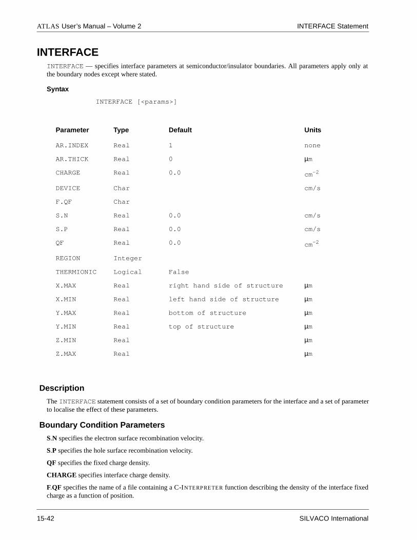
ATLAS User’s Manual – Volume 2 INTERFACE Statement
only at
rameter
d
INTERFACEINTERFACE — specifies interface parameters at semiconductor/insulator boundaries. All parameters apply the boundary nodes except where stated.
Syntax
INTERFACE [<params>]
Description
The INTERFACE statement consists of a set of boundary condition parameters for the interface and a set of pato localise the effect of these parameters.
Boundary Condition Parameters
S.N specifies the electron surface recombination velocity.
S.P specifies the hole surface recombination velocity.
QF specifies the fixed charge density.
CHARGE specifies interface charge density.
F.QF specifies the name of a file containing a C-INTERPRETER function describing the density of the interface fixecharge as a function of position.
Parameter Type Default Units
AR.INDEX Real 1 none
AR.THICK Real 0 µm
CHARGE Real 0.0 cm-2
DEVICE Char cm/s
F.QF Char
S.N Real 0.0 cm/s
S.P Real 0.0 cm/s
QF Real 0.0 cm-2
REGION Integer
THERMIONIC Logical False
X.MAX Real right hand side of structure µm
X.MIN Real left hand side of structure µm
Y.MAX Real bottom of structure µm
Y.MIN Real top of structure µm
Z.MIN Real µm
Z.MAX Real µm
15-42 SILVACO International

INTERFACE Statement Statements
THERMIONIC specifies that carrier transport across the interface by determined by thermionic emission. See theBLAZE Chapter for details. This parameter applied only at semiconductor/semiconductor boundaries.
AR.INDEX specifies the real component refractive index for the anti-reflective coating model in LUMINOUS. Thismodel assumes the imaginary component of refractive index is zero so that the layer is non-absorbing. This model isonly applicable for normal illumination.
AR.THICK specifies the thickness of an anti-reflective coating layer for the reflection model in LUMINOUS. Thislayer should generally not exist in the device mesh structure.
Position Parameters
X.MIN, X.MAX, Y.MIN, and Y.MAX define a bounding box. Any semiconductor/insulator interfaces found withinthis region are charged. If there is only one interface in a device, a nonplanar surface may be defined using a boxwhich contains the whole device
X.MIN specifies the left x-coordinate of the bounding box.
X.MAX specifies the right x-coordinate of the bounding box.
Y.MIN specifies the bottom y-coordinate of the bounding box.
Y.MAX specifies the top y-coordinate of the bounding box.
Z.MIN specifies the front z-coordinate of the bounding box. It is used in 3-D modules only.
Z.MAX specifies the back z-coordinate of the bounding box. It is used in 3-D modules only.
DEVICE specifies which device in a MIXEDMODE simulation the statement applies to
REGION specifies which the region number the statement applies to.
MOS Example
This example defines an interface with both fixed charge and recombination velocities.
INTERFACE X.MIN=-4 X.MAX=4 Y.MIN=-0.5 Y.MAX=4 \
QF=1E10 S.N=1E4 S.P=1E4
SOI Example
To define different fixed charge on the front and back interfaces of an SOI transistor two INTERFACE statements are
required. In the syntax below the first statement will apply 5.1010 cm-2 charge to any silicon/oxide interface aboveY=0.01µm. The second statement applied a higher charge to any interface below Y=0.01µm. Note that charges areonly applied at the material interfaces so the Y-coordinate needs only to be somewhere within the silicon film.
INTERFACE Y.MAX-0.01 QF=5e10
INTERFACE Y.MIN=0.01 QF=2e11
Interface Charge for III-V Devices
Interface charge can be at the interfaces between two semiconductor regions or at the edges of semiconductor regions using the CHARGE parameter. The location of the added charge can be controlled using the Position Parameters described above.
SILVACO International 15-43

ATLAS User’s Manual – Volume 2 INTTRAP Statement
tor and
/
band and
INTTRAPINTTRAP — activates interface defect traps at discrete energy levels within the bandgap of the semiconducsets their parameter values.
Syntax
INTTRAP <type> E.LEVEL=<r> DENSITY=<r> <capture parameters>
Description
DEVICE specifies which device the statement applies to in MIXEDMODE simulation.
DONOR specifies a donor-type trap level.
ACCEPTOR specifies an acceptor-type trap level.
DEGEN.FAC specifies the degeneracy factor of the trap level used to calculate the density.
DENSITY sets the maximum density of states of the trap level.
F.DENSITY specifies the name of a file containing a C-INTERPRETER function describing the density of donoracceptor interface traps as a function of position.
E.LEVEL sets the energy of the discrete trap level. It is equal to the energy distance between conductance trap level for acceptor trap, and to energy distance between trap level and valence band for donor trap.
Parameter Type Default Units
ACCEPTOR Logical False
DEGEN.FAC Real 1
DENSITY Real cm-2
DEVICE Char
DONOR Logical False
E.LEVEL Real eV
F.DENSITY Char
REGION Integer
SIGN Real cm2
SIGP Real cm2
TAUN Real s
TAUP Real s
15-44 SILVACO International

INTTRAP Statement Statements
Capture Parameters
Either the cross section or lifetime parameters should be used to define the capture parameters.
SIGN speccifies the capture cross section of the trap for electrons.
SIGP specifies the capture cross section of the trap for holes.
TAUN specifies the lifetime of electrons in the trap level.
TAUP specifies the lifetime of holes in the trap level.
Example setting Multiple Interface Trap States
The following example sets three discrete interface trap levels within the silicon bandgap. These trap levels willcapture carriers, slowing the switching speed of any device. In this example the capture cross sections are used todefine the properties of each trap.
inttrap e.level=0.49 acceptor density=2.e10 degen=12 \
sign=2.84e-15 sigp=2.84e-14
inttrap e.level=0.41 acceptor density=1.e10 degen=12 \
sign=7.24e-16 sigp=7.24e-15
inttrap e.level=0.32 donor density=1.e10 degen=1 \
sign=1.00e-16 sigp=1.00e-17
Note: For semiconductor bulk trap levels, see the TRAP statement.
E.level for donor trap
E.level for acceptor trap
EC
Eta
EV
Etd
SILVACO International 15-45

ATLAS User’s Manual – Volume 2 LOAD Statement
er
riginal
aded
t in the
ad only
form an
ded to
LOADLOAD — loads previous solutions from files as initial guesses to other bias points.
Syntax
LOAD [ASCII|MASTER] [NO.CHECK] <files>
Description
ASCII specifies that any original PISCES format files read or written by this statement will be in an ASCII raththan in a binary format.
MASTER specifies that any files read by this statement will be in a standard structure file rather than the oPISCES format. If you are using TONYPLOT to plot simulation results, this parameter should be specified.
TWOD allows loading of a 2-D solution into a 3-D structure. Note : The values from the 2-D solution are louniformly in the Z direction.
NO.CHECK prevents checking material parameter differences between loaded binary files and the values securrent input file.
File Parameters
The LOAD statement requires that one of the following file parameter syntaxes be used.
LOAD INFILE=<filename>
or
LOAD IN1FILE=<filename> IN2FILE=<filename>
INFILE specifies a single input filename for solution data. This parameter should be used when you wish to loone solution which is the most common case.
IN1FILE specifies a filename for present solution data. Use this parameter if two input files are needed to perextrapolation for an initial approximation (i.e., the PROJECT parameter of the SOLVE statement).
IN2FILE specifies an input filename for previous solution data. Use this parameter if two input files are neeperform an extrapolation for an initial approximation (i.e., the PROJECT parameter of the SOLVE statement). Thesolution specified by this parameter is the first to be overwritten when new solutions are obtained.
Parameter Type Default Units
ASCII Logical False
INFILE Character
INIFILE Character
IN2FILE Character
MASTER Logical False
NO.CHECK Logical False
TWOD Logical False
15-46 SILVACO International

LOAD Statement Statements
Simple Save and Load Examples
This example saves and later loads master format solution file SOL.STR
SAVE OUTF=SOL.STR.
....
LOAD INFILE=SOL.STR MASTER
As before but using the SOLVE syntax
SOLVE OUTF=SOL.STR MASTER
..
LOAD INF=SOL.STR MASTER
When the save and load operations are not done within the same ATLAS run see the Note below.
Binary Format Example
Saving and loading using the binary format. This is quicker but these files cannot be plotted in TONYPLOT.
SOLVE OUTF=SOLVE_TMP
..
LOAD INF=SOLVE_TMP
Note: The function to calculate the difference between two files is now inside TONYPLOT. It has beendiscontinued from the LOAD statement
Note: The LOAD statement loads only the saved solution quantities into ATLAS. The mesh, electrodes,doping, regions, contact settings, material parameters, models and numerical methods must all bespecified in advance of any LOAD statement. See the Re-Initializing ATLAS section of the GettingStarted Chapter.
SILVACO International 15-47

ATLAS User’s Manual – Volume 2 LOG Statement
ted by
LOGLOG — allows all terminal characteristics of a run to be lsaved to a file. Any DC, transient or AC data generaSOLVE statements after the LOG statement is saved. Any parameters specified by the PROBE statement are also storedin the logfile. If a log file is already open, the open log file is closed and a new log file is opened.
Syntax
LOG [OUTFILE=<filename>] [MASTER] [acparams]
Parameter Type Default Units
ABCD.PARAM Logical False
APPEND Logical False
GAINS Logical False
H.PARAM Logical False
IMPEDANCE Real 50 ohms
INPORT Character
IN2PORT Character
J.ELECTRON Logical False
J.HOLE Logical False
LCOMMON Real 0 H
LGROUND Real 0 H
LIN Real 0 H
LOUT Real 0 H
MASTER Logical True
OFF Logical False
OLD Logical False
OUTPORT Character
OUT2PORT Character
OUTFILE Character
RCOMMON Real 0 ohms
RGROUND Real 0 ohms
RIN Real 0 ohms
ROUT Real 0 ohms
S.PARAM Logical False
SIM.TIME Logical False s
15-48 SILVACO International

LOG Statement Statements
File Output Parameters
OUTFILE specifies the log file that will be used to store DC, AC or transient I-V information.
MASTER specifies that AC data and I-V information will be saved in a standard structure file format. This is thedefault format.
J.ELECTRON specifies that electron currents are to be written into the log file.
J.HOLE specifies that hole currents are to be written into the log file.
APPEND specifies that the output I-V information should be appended to an existing log file. Care should be taken toensure that the existing log files contain the same type of data (eg. DC, AC, transient) as the subsequent SOLVEstatements.
OFF specifies that any currently open log file will be closed and log file output is discontinued.
OLD specifies that AC data and IV information will be saved in the original PISCES-II file format.
Synonym: PISCES
Note: The older ACFILE syntax is not supported and should not be used. AC results are stored in thefile specified by OUTFILE as long as the first SOLVE statement after the LOG statement contains ACanalysis.
RF Analysis Parameters
If S.PARAM, H.PARAM, Z.PARAM, GAINS or ABCD.PARAM is specified, the capacitance and conductance datawill be converted into the requested set of AC parameters.
S.PARAM elects s parameter analysis. For s-parameter analysis the user may also choose to set any of the parasiticelement parameters.
H.PARAM selects h parameter analysis.
Y.PARAM selects Y parameter analysis
Z.PARAM selects z parameter analysis.
ABCD.PARAM selects ABCD parameter analysis.
GAINS selects the calculation of several types of gains used in RF analysis139. These are the stability factor, unilateralpower gain (GUmax), maximum unilateral transducer power gain (GTmax), maximum available power gain (Gma)and the maximum stable power gain (Gms). The magnitude of H21 is also calculated.
IMPEDANCE specifies the matching impedance for s-parameter calculation.
INPORT specifies the electrode name for the primary input port used when performing any AC parametercalculations.
IN2PORT specifies the electrode name of the secondary input port.
WIDTH Real 1 microns
Y.PARAM Logical False
Z.PARAM Logical False
Parameter Type Default Units
SILVACO International 15-49

ATLAS User’s Manual – Volume 2 LOG Statement
OUTPORT specifies the electrode name for the output ports used when performing any AC -parameter calculations.
OUT2PORT specifies the electrode n of the secondary output port
Parasitic Element Parameters
For RF parameter extraction, the user may also set any of the parasitic element parameters. By setting the parasiticelement parameters, the user can apply lumped parasitic resistances or inductances to the terminal of the two-portdevice during the RF parameter extraction. These parameters will not affect the capacitance or conductance matricescalculated by ATLAS.
RIN specifies the lumped parasitic resistance on the input to the two port device for s-parameter extraction. The valueof RIN is in Ohms.
ROUT specifies the lumped parasitic resistance on the output to the two port device for s-parameter extraction. Thevalue of ROUT is in Ohms.
RGROUND specifies the lumped parasitic resistance on the ground or common side of the two port device for s-parameter extraction. The value of RGROUND is in Ohms. RCOMMON is an alias for RGROUND.
LIN specifies the lumped parasitic inductance on the input to the two port device for s-parameter extraction. The valueof LIN is in Henrys.
LOUT specifies the lumped parasitic inductance on the output to the two port device for s-parameter extraction. Thevalue of LOUT is in Henrys.
LGROUND specifies the lumped parasitic inductance on the ground or common side of the two port device for s-parameter extraction. The value of LGROUND is in Henris. LCOMMON is an alias for LGROUND.
SIM.TIME saves the time taken for a bias point into the log file and measured in seconds. Note that if multiple jobsare using the same cpu that this method may not be a true reflection of processor speed.
WIDTH specified an output width (in z-direction) to apply during the s-parameter calculation. Note that thisparameter affects only the derived RF parameters and not currents, capacitances or conductances. The WIDTHparameter of the MESH statement can be used to scale these. Using both these WIDTH parameters will lead to amultiplication of the two widths for the RF parameters.
Simple Logfile Defintion Example
This example saves all I-V data in file myfile.log
LOG OUTF=myfile.log
Results should be plotted using TONYPLOT.
RF Analysis Example
To generate s-parameters assuming the input is gate/source and the output is drain/source. A width of 100 microns isalso defined along with 100ohm resistance on the input:
LOG OUTF=mysparams.log S.PARAM INPORT=gate OUTPORT=drain \ IN2PORT=source OUT2PORT=source WIDTH=100 RIN=100
Transient or AC Logfile Example
The contents of LOG files varies for different types of simulations (eg. DC, transient, AC). The content is set by thefirst SOLVE statement after the LOG statement. Therefore the following syntax is required
SOLVE VDRAIN=0.5
LOG OUTF=myfile.log
SOLVE VDRAIN=3.0 RAMPTIME=1e-9 DT=1e-11 TSTOP=1e-7
15-50 SILVACO International

LOG Statement Statements
Correct transient parameters would not have been stored if the LOG statement had been placed before the first SOLVEstatement which is DC.
SILVACO International 15-51

ATLAS User’s Manual – Volume 2 LX.MESH, LY.MESH Statement
LX.MESH, LY.MESHL<n>.MESH — specifies the location of grid lines along the <n>-axis in a rectangular mesh used in LASER simulation.The syntax is equivalent for x and y directions.
Syntax
LX.MESH NODE=<n> LOCATION=<n>
Description
NODE specifies the mesh line index. These mesh lines are assigned consecutively.
LOCATION specifies the location of the grid line.
LASER Mesh Example
This syntax defines a mesh of 33x33 covering the area bounded by (0.3,0.0) to (2.4,1.0)
LX.M n=1 l=0.3
LX.M n=33 l=2.4
LY.M n=1 l=0.0
LY.M n=33 l=1.0
Note: The mesh defined in these statements for the LASER Helmholtz Solver is entirely separate fromthe electrical device simulation mesh defined on the MESH statement.
Parameter Type Default Units
LOCATION Real µm
NODE Integer
15-52 SILVACO International

MATERIAL Statement Statements
standard
MATERIALMATERIAL — associates physical parameters with materials in the mesh. The parameter default values for semiconductors are shown in Appendix B.
Syntax
MATERIAL <localization> <material_definition>
Parameter Type Default Units
AFFINITY Real see Appendix B eV
ALIGN Real use AFFINITY
ALPHAA Real 0.0
ALPHAR Real 4.0
ARICHN Real see Appendix B A/cm2/K2
ARICHP Real see Appendix B A/cm2/K2
ASYMMETRY Real 0.5
AUGN Real see Appendix B cm6/s
AUGP Real see Appendix B cm6/s
AUGKN Num 0.0 cm3
AUGKP Num 0.0 cm3
BGN.C Real 0.5
BGN.N Real 1.0x1017 cm-3
BGN.E Real 9.0x10⁻³ V
COPT Real 0.0 cm3/s
DEVICE Character
EAB Real 0.045 eV
EDB Real 0.044 eV
EG300 Real see Appendix B eV
EGALPHA Real see Appendix B eV
EGBETA Real see Appendix B K
ETRAP Real 0.0 eV
EPSINF Real eV/K
F.ALPHAA Character
F.TAUN Character
SILVACO International 15-53
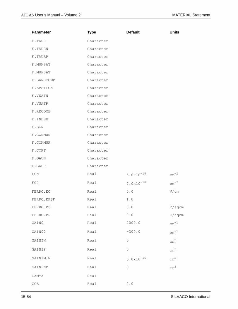
ATLAS User’s Manual – Volume 2 MATERIAL Statement
F.TAUP Character
F.TAURN Character
F.TAURP Character
F.MUNSAT Character
F.MUPSAT Character
F.BANDCOMP Character
F.EPSILON Character
F.VSATN Character
F.VSATP Character
F.RECOMB Character
F.INDEX Character
F.BGN Character
F.CONMUN Character
F.CONMUP Character
F.COPT Character
F.GAUN Character
F.GAUP Character
FCN Real 3.0x10⁻¹⁸ cm-2
FCP Real 7.0x10⁻¹⁸ cm-2
FERRO.EC Real 0.0 V/cm
FERRO.EPSF Real 1.0
FERRO.PS Real 0.0 C/sqcm
FERRO.PR Real 0.0 C/sqcm
GAIN0 Real 2000.0 cm-1
GAIN00 Real -200.0 cm-1
GAININ Real 0 cm2
GAINIP Real 0 cm2
GAIN1MIN Real 3.0x10⁻¹⁶ cm2
GAIN2NP Real 0 cm5
GAMMA Real
GCB Real 2.0
Parameter Type Default Units
15-54 SILVACO International

MATERIAL Statement Statements
G.SURF Real 1.0 cm2
GVB Real 4.0
G.CONDUCTIVITY Real
HC.A Real See Appendix B J/Kcm3
HC.B Real See Appendix B J/K2cm3
HC.C Real See Appendix B J/Kcm3
HC.D Real See Appendix B JKcm3
IMAG.INDEX Real See Appendix B
INDEX.FILE Character
KLASRH Logical False
KLAAUG Logical False
KSRHTN Real 2.5x10⁻³ s
KSRHTP Real 2.5x10⁻³ s
KSRHCN Real 3.0x10⁻¹³ cm3
KSRHCP Real 11.76x10⁻¹³ cm3
KSRHGN Real 1.77
KSRHGP Real 0.57
KAUGCN Real 1.83x10⁻³¹ cm6/s
KAUGCP Real 2.78x10⁻³¹ cm6/s
KAUGDN Real 1.18
KAUGDP Real 0.72
LT.TAUN Real 0.0
LT.TAUP Real 0.0
MASS.VTHN Real 0.0
MASS.VTHP Real 0.0
MATERIAL Character
MUN Real See Appendix B
MUP Real See Appendix B
NAME Character
NC300 Real See Appendix B cm-3
Parameter Type Default Units
SILVACO International 15-55

ATLAS User’s Manual – Volume 2 MATERIAL Statement
NSRHN Real See Appendix B cm-3
NSRHP Real See Appendix B cm-3
NUE.EXTR Real
NUH.EXTR Real
NV300 Real See Appendix B cm-3
OXCH.ONLY Logical False
PERMITTIVITY Real See Appendix B F/cm
POWER Real
REAL.INDEX Real See Appendix B
REGION All regions
SEMICONDUC Logical False
TAUMOB.EL Real 0.4x10⁻¹² s
TAUMOB.HO Real 0.4x10⁻¹² s
TAUN0 Real See Appendix B s
TAUP0 Real See Appendix B s
TAUREL.EL Real 0.4x10⁻¹² s
TAUREL.HO Real 0.4x10⁻¹² s
TC.A Real See Appendix B (cm·K)/W
TC.B Real See Appendix B cm/WK
TC.C Real See Appendix B cm/WK
TC.C0 Real
TC.NPOW Real
TC.E Real
TC.D Real
TCON.CONST Logical
TCON.POWER Logical
TCON.POLYNOM Logical
TCON.RECIPRO Logical
TMUN Real
TMUP Real
TRE.T1 Real s
Parameter Type Default Units
15-56 SILVACO International

MATERIAL Statement Statements
Description
The MATERIAL statment is used set basic material parameters related to band structure and parameters for certainmobility, recombination or carrier statistics models. Parameters for temperature dependence are noted in a separatesection below.
Localization of Material Parameters
DEVICE specifies which device the MATERIAL statement should apply to in MIXEDMODE simulation.
MATERIAL specifies which material from the table in Appendix B that the MATERIAL statement should apply. If amaterial is specified, then all regions defined as being composed of that material will be affected.
NAME specifies which region the MATERIAL statement should apply. Note that the name must match the namespecified in the NAME parameter of the REGION statement.
REGION specifies the region number to which these parameters apply. If there is more than one semiconductorregion, specification of different parameters for each region is allowed. If REGION is not specified, all regions in thestructure are changed.
Band Structure Parameters
AFFINITY specifies the electron affinity.
ALIGN specifies the fraction of the bandgap difference that is applied to the conduction band edge, relative to theminimum bandgap material in the device. Note that specifying this parameter overrides any electron affinityspecification. See the BLAZE chapter for notes on setting the band alignment.
TRE.T2 Real s
TRE.T3 Real s
TRE.W1 Real eV
TRE.W2 Real eV
TRE.W3 Real eV
TRH.T1 Real s
TRH.T2 Real s
TRH.T3 Real s
TRH.W1 Real eV
TRH.W2 Real eV
TRH.W3 Real eV
VSAT Real cm/s
VSATN Real cm/s
VSATP Real cm/s
VSATURATION Real cm/s
VTHN Real See Appendix B cm/s
VTHP Real See Appendix B cm/s
Parameter Type Default Units
SILVACO International 15-57
ATLAS User’s Manual – Volume 2 MATERIAL Statement
ARICHN specifies the effective Richardson constant for electrons.
ARICHP specifies the effective Richardson constant for holes.
EG300 specifies energy gap at 300K (see Equation 3-36).All semiconductor materials in ATLAS must have a definedEG300.
F.BANDCOMP specifies the name of a file containing a C-INTERPRETER funciton for the specification oftemperature and composition dependent band parameter models.
F.EPSILON specifies the name of a file containing a C-INTERPRETER function for the specification of temperatureand composition dependent static dielectric constant models.
MASS.VTHN specifies the electron effective mass for calculation of thermal velocity in the thermionicheterojunction model (see Equation 5-45).
MASS.VTHP specifies the hole effective mass for calculation of thermal velocity in the thermionic heterojunctionmodel (see Equation 5-46).
NC300 specifies the conduction band density at 300K. (see Equation 3-29).
NV300 specifies valence band density at 300K (see Equation 3-30).
PERMITTIVITY specifies dielectric permittivity of the material. All materials in an ATLAS structure must have adefined permittivity.
Mobility Model Parameters
F.CONMUN specifies the name of a file containing a C-INTERPRETER function for the specification of temperature,composition and doping dependent electron mobility models.
F.CONMUP specifies the name of a file containing a C-INTERPRETER function for the specification of temperature,composition and doping dependent hole mobility models.
F.MUNSAT specifies the name of a file containing a C-INTERPRETER function for the specification of parallel fielddependent electron mobility model for velocity saturation.
F.MUPSAT specifies the name of a file containing a C-INTERPRETER function for the specification of parallel fielddependent hole mobility model for velocity saturation.
F.VSATN specifies the name of a file containing a C-INTERPRETER function for the specification of temperature andcompostion dependent electron saturation velocity models.
F.VSATP specifies the name of a file containing a C-INTERPRETER function for the specification of temperature andcompostion dependent hole saturation velocity models.
GSURF specifies a factor by which mobility is reduced at the semiconductor surface.This is a simple but not accuratealternative to the transverse field dependent or surface mobility models set on the MODELS statement.
MUN specifies low-field electron mobility. This parameter is only used if no concentration dependent mobility modelis specified.
MUP specifies low-field hole mobility.This parameter is only used if no concentration dependent mobility model isspecified.
VSATURATION specifies the saturation velocity for the electric field dependent mobility.
VSATN specifies the saturation velocity for electrons.
VSATP specifies the satruation velocity for holes.
Recombination Model Parameters
AUGN specifies the Auger coefficient cn (see Equation 3-227).
AUGP Specifies the Auger coefficient cp (see Equation 3-227).
15-58 SILVACO International

MATERIAL Statement Statements
AUGKN parameter of the narrow band-gap electron Auger recombination coefficient model.
AUGKP parameter of the narrow band-gap electron Auger recombination coefficient model.
COPT specifies the optical recombination rate for the material. This parameter has no meaning unless MODELSOPTR has been specified (see Equation 3-226).
ETRAP specifies the trap energy for SRH recombination
F.COPT specifies the name of a file containing a C-INTERPRETER function for the specification of composition andtemperature dependence of the radiative recombination rate.
F.GAUN specifies the name of a file containing a C-INTERPRETER function for the specification of composition andtemperature dependence of the electron Auger coefficient.
F.GAUP specifies the name of a file containing a C-INTERPRETER function for the specification of composition andtemperature dependence of the hole Auger coefficient.
F.TAUN specifies the name of a file containing a C-INTERPRETER function for the specification of positiondependent electron lifetime models.
F.TAUP specifies the name of a file containing a C-INTERPRETER function for the specification of positiondependent hole lifetime models.
F.TAURN specifies the name of a file containing a C-INTERPRETER function specifying the electron relaxation timeas a function of electron energy.
F.TAURP specifies the name of a file containing a C-INTERPRETER function specifying the hole relaxation time as afunction of hole energy.
F.RECOMB specifies the name of a file containing a C-INTERPRETER function for the specification of temperature,composition, electron and hole concentration dependent recombination rate models.
KLASRH and KLAAUG Model parameters
KSRHTN coefficient for Klaassen’s concentration and temperature dependent SRH lifetime model.
KSRHTP coefficient for Klaassen’s concentration and temperature dependent SRH lifetime model.
KSRHCN coefficient for Klaassen’s concentration and temperature dependent SRH lifetime model.
KSRHCP coefficient for Klaassen’s concentration and temperature dependent SRH lifetime model.
KSRHGN coefficient for Klaassen’s concentration and temperature dependent SRH lifetime model.
KSRHGP coefficient for Klaassen’s concentration and temperature dependent SRH lifetime model.
KAUGCN coefficient for Klaassen’s concentration dependent Auger model.
KAUGCP coefficient for Klaassen’s concentration dependent Auger model.
KAUGDN coefficient for Klaassen’s concentration dependent Auger model.
KAUGDP coefficient for Klaassen’s concentration dependent Auger model.
NSRHN specifies the SRH concentration parameter for electrons (see Equation 3-215).
NSRHP specifies the SRH concentration parameter for holes (see Equation 3-216).
TAUN0 specifies SRH lifetime for electrons (see Equation 3-215).
TAUP0 specifies SRH lifetime for holes (see Equation 3-216).
VTHN specifies the thermal velocity for electrons for use in TRAP recombination.
VTHP specifies the thermaln velocity for holes for use in TRAP recombination.
SILVACO International 15-59

ATLAS User’s Manual – Volume 2 MATERIAL Statement
Carrier Statistics Model Parameters
ASYMMETRY specifies the relative degree to which band gap narrowing applies to the conduction band versus thevalence band. The value of the ASYMMETRY parameter is multiplied by the total change in band gap due to band gapnarrowing and that product is applied to the conduction band edge. For example, if the ASYMMETRY parameter has avalue of 1.0 then the change in band gap due to band gap narrowing is applied only to the conduction band edge andthe valence band edge remains unaffected.
BGN.E, BGN.N and BGN.C specify the parameters of the band gap narrowing model given in Equation 3-38.
EAB specifies acceptor energy level (see Equation 3-44).
EDB specifies donor energy level (see Equation 3-43).
F.BGN specifies the name of a file containing a C-INTERPRETER function for the specification of temperature,composition and doping dependent bandgap narrowing models.
GCB specifies the conduction-band degeneracy factor (see Equation 3-43).
GVB specifies the valence-band degeneracy factor (see Equation 3-44).
Energy Balance Parameters
TAUMOB.EL specifies the relaxation time for electrons in the temperature dependent mobility model.
TAUMOB.HO specifies the relaxation time for holes in the temperature dependent mobility model .
TAUREL.EL specifies the relaxation time for electrons in the energy balance model (see Equation 3-95).
TAUREL.HO specifies the relaxation time for holes in the energy balance model (see Equation 3-96).
TRE.T1, TRE.T2, TRE.T3, TRE.W1, TRE.W2, TRE.W3, TRH.T1, TRH.T2, TRH.T3, TRH.W1, TRH.W2, andTRH.W3 are used in the temperature dependent energy relaxation time model based on table data from Laux-FischettiMonte-Carlo simulation (see Table 3-9).
Lattice Temperature Dependence Parameters
EGALPHA specifies the alpha coefficient for temperature dependence of bandgap (see Equation 3-36).
EGBETA specifies the beta coefficient for temperature dependence of bandgap (see Equation 3-36).
HC.A, HC.B, HC.C, and HC.D specify the values of the four coefficient of the heat capacity equation (see Equation6-6).
LT.TAUN specifies the temperature dependence for electron lifetimes (see Equation 6-9).
LT.TAUP specifies the temperature dependence for hole lifetimes (see Equation 6-20).
POWER specifies the value of thermal power generated in a power source associated with a region in THERMAL3D.
TC.A, TC.B, and TC.C specify the three thermal conductivity coefficients (see Equation 6-4).
TC.C0 specifies the equilibrium value of thermal conductivity, k(T0), in equation 13-2.
Synonym: TC.CONST
TC.D specifies the value of the parameter D in equation 13-5.
TC.E specifies the value of the parameter E in equation 13-5.
TCON.CONST specifies that thermal conductivity should be modeled as constant with respect to temperature. Thevalue of the thermal conductivity is given by the value of the TC.C0 parameter.
TCON.POWER specifies that the temperature dependence of thermal conductivity should be modeled using equation13-3.
TCON.POLYNOM specifies that the temperature dependence of thermal conductivity should be modeled usingequation 13-4.
15-60 SILVACO International
MATERIAL Statement Statements
8-12).
eful tormat of
efaults
ot
TCON.RECIPRO specifies that the temperature dependence of thermal conductivity should be modeled usingequation 13-5.
TC.NPOW specifies the value of the coefficient of temperature dependence of thermal conductivity, n, in equation13-3.
TMUN and TMUP specify the temperature coefficients for the temperature dependence of electron lattice mobility,and of hole lattice mobility respectively.
Oxide Material Parameters.
SEMICONDUC specifies that an oxide region is to be treated as a semiconductor.
OXCH.ONLY specifies that electron and hole concentrations are omitted from Poisson’s equation in oxides.
Photogeneration Parameters.
F.INDEX specifies the name of a file containing a C-INTERPRETER function for the specification of wavelengthdependent complex index of refraction models.
IMAG.INDEX specifies the imaginary portion of the refractive index of the semiconductor (see Equation Wavelength dependent defaults exist for certain materials as documented in Appendix B.
INDEX.FILE specifies the filename from which refractive indices for a material are read. This parameter is usload wavelength dependent refractive indices for use with both mono- and multi- spectral light sources. The fothis file is:
<n>
wavelength(1) real index(1) imaginary index(1)
wavelength(2) real index(2) imaginary index(2)
...
wavelength(n) real index(n) imaginary index(n)
Where n is the number of lines to be read.
REAL.INDEX specifies the real portion of the refractive index of the semiconductor. Wavelength dependent dexist for certain materials as documented in Appendix B.
LASER Parameters
ALPHAA specifies the bulk absorption coeffiecient in Equation 9-2.
ALPHAR specifies the line width broadening factor in Equation 9-2.
EPSINF specifies the high frequency relative dielectric permittivity (ε∞) (see Equation 9-2). If this parameter is nspecified, it will be set equal to the static dielectric permittivity of the material.
F.ALPHAA specifies the name of a file containing a C-INTERPRETER function for the bulk absorption coeffiecient.
FCN parameter in the LASER free-carrier loss model.
FCP parameter in the LASER free-carrier loss model.
GAIN0 specifies the parameter g0 in Equations 9-3 and 9-11.
GAIN00 specifies the parameter g00 in Equation 9-6.
GAIN1N specifies the parameter g1n in Equation 9-6.
GAIN1P specifies the parameter g1p in Equation 9-6.
GAIN1MIN specifies the parameter g1min in Equation 9-6.
GAIN2NP specifies the parameter g2np in Equation 9-6.
SILVACO International 15-61

ATLAS User’s Manual – Volume 2 MATERIAL Statement
GAMMA specifies the parameter in Equation 9-3. If this parameter is not specified, it will be calculated usingEquation 9-5.
Material Coefficient Definition Examples
Numbered region
This example specifies SRH lifetimes and concentration independent low-field mobilities for region number 2. Allother parameters use default values and parameters in other regions are unaffected.
MATERIAL TAUN0=5.0E-6 TAUP0=5.0E-6 MUN=3000 MUP=500 REGION=2
All regions
This example defines carrier lifetimes and the refractive index for all semiconductor regions.
MATERIAL TAUP0=2.E-6 TAUN0=2.E-6 REAL.INDEX=3.7 \
IMAG.INDEX=1.0E-2
Named Material
This shows the definition of bandgap for all InGaAs regions in the structure:
MATERIAL MATERIAL=InGaAs EG300=2.8
Note: The command MODEL PRINT can be used to echo back default material parameters orMATERIAL parameter settings to the run-time output.
Note: All materials are divided into three classes: semiconductors, insulators and conductors. SeeAppendix B for important information about parameters required for each material class.
15-62 SILVACO International

MEASURE Statement Statements
MEASUREMEASURE — extracts selected electrical data from the solution.
Note: This statement is mostly obsolete and functions are replaced by the EXTRACT statement,OUTPUT statement or PROBE statement
Syntax
MEASURE <dt> [<boundary>] [OUTFILE=<filename>]
Parameter Type Default Units
CONTACT Integer
E.CRIT Real1E-8
ELECTRON Logical False
HOLE Logical False
IONIZINT Logical False
LRATIO Real 1.0
METAL.CH Logical False
N.CURRENT Logical False
N.LAYER Real 15
N.LINES Integer 50
N.RESIST Logical False
NET.CARR Logical False
NET.CHAR Logical False
OUTFILE Character
P.CURRENT Logical False
P.RESIST Logical False
REGIONS Integer All regions
SUBSTR Character
U.AUGER Logical False
U.RADIATIVE Logical False
U.SRH Logical False
U.TOTAL Logical False
X.MIN Real Left of device µm
SILVACO International 15-63

ATLAS User’s Manual – Volume 2 MEASURE Statement
er if a
Description
dt is one of the data type parameters described on the following page. These parameters are used to specify the type ofinformation to be measured.
boundary is one of the boundary parameters described on page 15-63. These parameters specify which nodes will bemeasured.
OUTFILE specifies a filename in which simulation results and bias information will be written.
Data Type Parameters
Net carrier concentration, charge concentration, electron concentration, or hole concentration may be integrated over asection of a device. The charge on part of an electrode can be calculated, as can the current through that part. This isuseful for capacitance studies in conjunction with the difference mode of the LOAD statement. The resistance of astructure cross-section, such as a diffused line, may be calculated.
E.CRIT specifies the critical electric field used to calculate integration integrals.
ELECTRON extracts integrated electron concentration.
HOLE extracts integrated hole concentration.
IONIZINT enable the calculation of ionization integrals. Other integral ionization parameters will be ignored unlessIONIZINT is specified.
LRATIO specifies the ratio between electric field lines used in ionization integral calculation. The value of thisparameter should be set from 0.5 to 1.5.
METAL.CH extracts integrated charge on a contact.
N.CURRENT extracts n-current through an electrode.
N.LINES specifies the number of ionization integrals.
N.RESIST extracts n-resistance of a cross-section.
NET.CARR extracts integrated carrier concentration.
NET.CHAR extracts integrated net charge.
NLAYERS controls the distance from the contact where electric field lines start.
P.CURRENT extracts p-current through an electrode.
P.RESIST extracts p-resistance of a cross-section.
SUBSTR selects the “substrate” electrode for electric field lines. You do not need to specify this paramet“substrate” electrode has been defined in the ELECTRODE statement.
U.AUGER specifies that the integrated Auger recombination rate is to be extracted.
U.RADIATIVE specifies that the integrated radiative recombination rate is to be extracted.
U.SRH specifies that the integrated SRH recombination rate is to be extracted.
U.TOTAL specifies that the integrated total recombination rate is to be extracted.
X.MAX Real Right of device µm
Y.MIN Real Top of device µm
Y.MAX Real Bottom of device µm
Parameter Type Default Units
15-64 SILVACO International

MEASURE Statement Statements
Boundary Parameters
Boundary parameters X.MIN, X.MAX, Y.MIN, and Y.MAX define a bounding box. Only nodes falling within thisbounding box are included in the integration. The default bounds are the boundaries of the entire device.
CONTACT specifies the contact number. For electrode quantities (current and metal charge) a contact must beselected. Only nodes falling within the bounds and belonging to the contact are included in the integration. WhenIONIZINT is specified, this is the electrode used to start electric field lines.
REGIONS specifies a particular set of regions. If REGIONS is specified, only nodes within the specified bounds thatare part of a particular set of regions will be integrated.
X.MAX specifies the x-coordinate of the right edge of the bounding box.
X.MIN specifies the x coordinate of the left edge of the bounding box.
Y.MAX specifies the y coordinate of the top of the bounding box.
Y.MIN specifies the y coordinate of the bottom of the bounding box.
Resistance Example
This example extracts the resistance of a p-type line diffused into a lightly doped n-substrate. Since the p-conductivityof the substrate is negligible, the integration bounds can include the whole device.
MEASURE P.RESIST
Gate Charge Example
In this example, the charge on the lower surface of a gate electrode is integrated. There is 0.05 µm of gate oxide on thesurface, which is located at y=0.
MEASURE METAL.CH CONT=1 X.MIN=-2.0 X.MAX=2.0 \
Y.MAX=-0.0499 Y.MIN=-0.0501
Ionization Integral Example
This example shows how to extract the maximum ionization integral in the device.
MEASURE IONIZINT CONTACT=3 SUSTR=4 N.LINES=200 \
NLAYERS=15 LRATIO=1.1
This syntax was the original implementation of ionization integrals in early ATLAS versions. It has been superceded.See the SOLVE and OUTPUT statements for the recommended approach to extract ionization integrals.
SILVACO International 15-65

ATLAS User’s Manual MESH Statement
is notical
MESHMESH — generates a mesh or reads a previously generated mesh.
Syntax
MESH <prev>|<new> [<output>]
Description
prev is a set of parameters that allow the user to read a previously generated mesh type.
new is a set of parameters that allow the user to initiate the generation of a rectangular mesh.
output is a set of the parameters for saving the mesh
Parameters related to reading in an existing mesh file
CYLINDRICAL specifies that the mesh being read in contains cylindrical symmetry. Since this information saved in the mesh file, the CYLINDRICAL parameter must be specified each time a structure with cylindrsymmetry is loaded.
FLIP.Y reverses the sign of the y coordinate.
INFILE specifies the name of a previously generated mesh that has been saved to disk.
Parameter Type Default Units
ATHENA Logical False
CYLINDRICAL Logical False
DIAG.FLIP Logical True
FLIP.Y Logical False
INFILE Character
MASTER.IN Logical True
MASTER.OUT Logical True
NX Integer
NY Integer
NZ Integer
OUTFILE Character
PISCES.IN Logical False
SCALEY Integer 1
SMOOTH.KEY Integer
SPACE.MULT Real 1.0
WIDTH Real 1.0
15-66 SILVACO International

MESH Statement Statements
MASTER.IN specifies a filename from which to read mesh and doping information in the SILVACO standardstructure file (SSF) format. This parameter is used to read in ATHENA or DEVEDIT structure files. Typically suchfiles contain all REGION, ELECTRODE and DOPING information although ATLAS allows users to modify thestructure using these statements.This parameter is true by default and is the only file format supported by Silvaco.
PISCES.IN indicates that the mesh file is in the old PISCES-II format. This is not recommended or supported bySilvaco.
SCALE.Y specifies a factor by which all x- and y-coordinates are multiplied.
SPACE.MULT is a scale factor that is applied to all specified grid spacings. This parameter can be used to produce acoarse mesh and therby reduce the simulation time.
ATHENA reads mesh and doping data generated by the ATHENA PISCES-II format file. This parameter and fileformat is obsolete.
Parameters Related to Creation of a New Mesh
RECTANGULAR initiates the generation of a rectangular mesh.
CYLINDRICAL specifies that the mesh contains cylindrical symmetry. Since this information is not saved in themesh file, the CYLINDRICAL parameter must be specified each time a grid with cylindrical symmetry is loaded.Structures defined as cylindrical will be rotated 360 degress about the y-axis. The coordinate x=0 must be on theextreme left hand side of the structure.
DIAG.FLIP flips the diagonals in a square mesh about the center of the grid. If the parameter is negated using^DIAG.FLIP is specified, all diagonals will be in the same direction.
NX specifies the number of nodes in the x direction.
NY specifies the number of nodes in the y direction.
NZ specifies the number of nodes in the z direction, used in DEVICE3D or BLAZE3D only.
WIDTH specifies a scale factor to represent the unsimulated dimension for 2-D simulations. This scale factor isapplied to all run time and log file outputs.
Output Parameters
OUTFILE specifies the output filename to which the mesh is written.
MASTER.OUT specifies the format of the output file. This parameter is true by default so the output file willconform to SILVACO Standard Structure File Format and can be plotted in TONYPLOT.
SMOOTH.KEY specifies a smoothing index. The digits of the index are read in reverse order and interpreted asfollows:
1. Triangle smoothing. All region boundaries remain fixed.
2. Triangle smoothing. Only material boundaries are maintained.
3. Node averaging.
4. Improved triangle smoothing method. This method uses diagonal flipping to reduce the number of obtuse triangles.
5. Triangle smoothing by flipping diagonals according to electric field.
Usually option 1 is sufficient. Option 2 is useful only if a device has several regions of the same material and theborder between different regions is unimportant. Option 3 is not recommended when the initial mesh is basicallyrectangular, such as mesh information usually obtained from SSUPREM4. Option 4 is similar to option 1, but option4 usually creates less obtuse triangles.
Mesh Definition Example
This example initiates a rectangular mesh and stores the mesh in file MESH1.STR.
SILVACO International 15-67

ATLAS User’s Manual MESH Statement
MESH RECTANGULAR NX=40 NY=17 OUTF=MESH1.STR
ATHENA Interface Example
This syntax reads in a mesh from ATHENA or DEVEDIT:
MESH INFILE=NMOS.STR
When the auto- interface feature is used in DECKBUILD the program will automatically insert the MESH statement toload the result of previous programs into ATLAS.
Note: Please see the Getting Started Chapter or the on-line examples for details of the interfaces fromATHENA or DEVEDIT to ATLAS
15-68 SILVACO International

METHOD Statement Statements
the these
METHODMETHOD — sets the numerical methods to be used to solve the equations and parameters associated withalgorithms.
Syntax
METHOD <gp> <mdp>
Parameter Type Default Units
2NDORDER Logical True
ATRAP Real 0.5
AUTONR Logical False
BIGGEST Logical False
BLOCK Logical True
CARRIERS Real 2
C.ITLIMIT Integer 500
C.STABIL Real 1.0x10⁻¹⁰
C.RESID Real 1.0x10⁻⁸
CLIM.DD Real 4.5x1013 cm-3
CLIM.EB Real 0 cm-3
CLIMIT Real 10000
CR.TOL Real 5.0x10⁻¹⁸
CUR.PROJ Logical False
CX.TOLER Real 1.0x10⁻⁵
DIRECT Logical False
DT.MAX Real ∞
DT.MIN Real 1.0x10⁻²⁵ s
DVLIMIT Real 0.1
DVMAX Real 2.5 V
ELECTRONS Logical True
EXTRAPOLATE Logical False
FIX.QF Logical False
GMRES Logical False
GUM.INIT Integer 15
SILVACO International 15-69
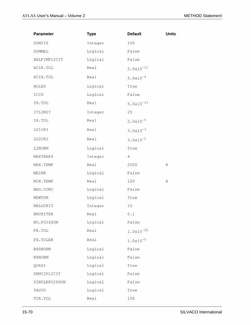
ATLAS User’s Manual – Volume 2 METHOD Statement
GUMITS Integer 100
GUMMEL Logical False
HALFIMPLICIT Logical False
HCIR.TOL Real 5.0x10⁻¹¹
HCIX.TOL Real 5.0x10⁻⁴
HOLES Logical True
ICCG Logical False
IR.TOL Real 5.0x10⁻¹⁵
ITLIMIT Integer 25
IX.TOL Real 2.0x10⁻⁵
LU1CRI Real 3.0x10⁻³
LU2CRI Real 3.0x10⁻²
L2NORM Logical True
MAXTRAPS Integer 4
MAX.TEMP Real 2000 K
MEINR Logical False
MIN.TEMP Real 120 K
NEG.CONC Logical False
NEWTON Logical True
NBLOCKIT Integer 15
NRCRITER Real 0.1
NO.POISSON Logical False
PR.TOL Real 1.0x10⁻²⁶
PX.TOLER Real 1.0x10⁻⁵
RHSNORM Logical False
RXNORM Logical False
QUASI Logical True
SEMIIPLICIT Logical False
SINGLEPOISSON Logical False
TAUTO Logical True
TCR.TOL Real 100
Parameter Type Default Units
15-70 SILVACO International

METHOD Statement Statements
Description
The METHOD statement is used to set the numerical methods for subsequent solutions. All structure and modeldefintions should precede the METHOD statement and all biasing conditions should follow it.Parameters on theMETHOD statement are used to set the solution technique, specify options for each technique and tolerances forcovergence.
Parameters to select the Solution Method
Note: Details of the different solution methods can be found in the Numerical Techniques Chapter
BLOCK specifies that the block Newton solution method will be used as a possible solution method in subsequentsolve statements until otherwise specified.The BLOCK method only has meaning when either lattice heating or energybalance is included in the simulation. For isothermal drift diffusion simulations BLOCK is equivalent to NEWTON.
BICGST switches from the default ILUCGS iterative solver to the BICGST interative solver for 3-D simulations.
DIRECT specifies that a direct linear solver should be used to solve the linear problem during 3-D simulation. Bydefault the ILUCGS iterative solver is used for 3-D problems.
GMRES switches from the default ILUCGS iterative solver to the GMRES interative solver for 3-D simulations.
GUMMEL specifies the Gummel method will be used as a solution method in subsequent SOLVE statements untilotherwise specified. If other methods (BLOCK or NEWTON) are specified in the same METHOD statement, each solutionmethod will be applied in succession until convergence is obtained. The order that the solution methods will beapplied is GUMMEL then BLOCK then NEWTON. If no solution methods are specified NEWTON is applied by default.
HALFIMPLICIT specifies that a semi-implicit scheme will be used for transient solutions in 3-D. In most cases thismethod is significantly less time consuming that the default TR-BDG method.
TCX.TOL Real
TLR.TOL Real 100
TLX.TOL Real
TMIN.FACT Real 0.4
TOL.LTEMP Real 0.001
TOL.RELAX Real 1
TOL.TIME Real 5.0x10⁻³
TRAP Logical True
TSETP.INCR Real 2.0
V.TOL Real 1.0x10⁻⁶
VSATMOD.INC Real 0.01
XNORM Logical False
WEAK Real 200
Parameter Type Default Units
SILVACO International 15-71

ATLAS User’s Manual – Volume 2 METHOD Statement
ed.If no
e 0, 1
Theld not
vergence
eters
L and
This ishis.
ion.
MEINR specifies the Meinerzhagens method whereby carrier temperature equations will be coupled with theassociated carrier continuity equation will be used during GUMMEL iterations.
NEWTON specifies that Newton’s method will be used as the solution method in subsequent SOLVE statements untilotherwise specified.Certain models and boundary conditions settings require that Newton’s method is ussolution methods are specified NEWTON is applied by default.
Parameters to select which equations are solved
CARRIERS specifies the number of carrier continuity equations that solutions will be found for. Valid values arand 2. CARRIERS=0 implies that only Poisson’s equation is solved for. CARRIERS=1 implies that only one carriersolution will be obtained. When this is specified one should also specify either HOLES or ELECTRONS.CARRIERS=2 implies that solutions will be obtained for both electrons and holes.
ELECTRONS specifies that only electrons will be simulated for single carrier simulation. .
HOLES specifies that only holes will be simulated for single carrier simulations.
Solution Tolerance Parameters
Note: Generally the solution tolerances should not be changed. Convergence problems should betackled by improving the mesh or checking the model and method combinations. The Getting StartedChapter has useful hints.
The default convergence criteria used in ATLAS consists of a combination of relative and absolute values. program will converge if either criterion is met. This is particularly useful when low-carrier concentrations wouconverge using just relative criteria.
Current convergence criteria are also used. Terminal currents are monitored at each iteration and overall conis allowed if currents converge along with absolute potential error.
CR.TOL specifies an absolute tolerance for the continuity equation.
CX.TOL or C.TOL is the relative tolerance for the continuity equation. The XNORM parameter uses paramCX.TOL and PX.TOL to calculate convergence criteria.
HCIR.TOL is the absolute current convergence criteria for energy transport models.
HCIX.TOL is the relative current convergence criteria for energy transport models.
IR.TOL specifies absolute current convergence criteria.
IX.TOL specifies relative current convergence criteria.
PR.TOL specifies an absolute tolerance for the Poisson equation.
PX.TOL is the relative tolerance for the potential equation. The XNORM parameter uses parameters CX.TOPX.TOL to calculate convergence criteria.
RHSNORM specifies that only absolute errors will be used to determine convergence. If RHSNORM is selectedPoisson error are measured in C/µm and the continuity error is measured in A/µm.
RXNORM specifies that both relative and absolute convergence criteria will be used in the solution method.the equivalent of specifying both XNORM and RHSNORM. This is the default and it is not recommended to change t
TCR.TOL specifies the absolute (RHS norm) tolerance for convergence of the carrier temperature equations.
TCX.TOL specifies the relative (X norm) tolerance for convergence of the carrier temperature equations.
TOL.TIME specifies maximum local truncation error for transient simulations.
TOL.LTEMP specifies the temperature convergence tolerance in block iterations using the lattice heat equat
15-72 SILVACO International

METHOD Statement Statements
dates.
ximation
n theear
TOL.RELAX specifies a relaxation factor for all six Poisson, continuity, and current convergence parameters(PX.TOL, CX.TOL, PR.TOL, CR.TOL, IX.TOL, and IR.TOL).
TLR.TOL specifies the relative (X norm) tolerance for convergence of the lattice temperature equation.
TLX.TOL specifies the relative (X norm) tolerance for convergence of the lattice temperature equation.
WEAK specifies the multiplication factor for weaker convergence tolerances applied when current convergence isobtained.
XNORM specifies that only the relative errors will be used to determine convergence for the drift-diffusionequations. If XNORM is used Poisson updates are measured in kT/q. and carrier updates are measured relative to thelocal carrier concentration.
General Parameters
ATRAP specifies the multiplication factor which reduces the electrode bias steps when a solution starts to diverge.This parameter has no effect unless the TRAP parameter is specified.
CLIM.DD is analogous to CLIMIT except it is expressed in a dimensional value representing the minimum carrierconcentration that can be resolved.
CLIM.EB can be treated as a regularization parameter for the case of very small carrier concentrations for energybalance simulation. It specifies the minimum value of carrier concentration for which the relaxation term in the energybalance equation will still be properly resolved. Carrier temperatures for points where the concentration is much lessthan CLIM.EB, will tend to the lattice temperature.
CLIMIT specifies a concentration normalization factor. See the Numerical Techniques chapter for a completedescription.
CUR.PROJ enables the use of projection method for initial guesses with current boundary conditions.
FIX.QF fixes the quasi-Fermi potential of each non-solved for carrier to a single value, instead of picking a valuebased on local bias.
ITLIMIT or GITLIMIT specifies the maximum number of allowed outer loops (Newton loops or Gummelcontinuity iterations).
MAXTRAPS specifies the number of times the trap procedure will be repeated in case of divergence. The value ofMAXTRAPS may range from 1 to 10.
MIN.TEMP and MAX.TEMP are specified to control the absolute range of lattice temperatures allowed duringGummel loop iterations with lattice temperature. These parameters help insure that lattice temperatures convergeduring the outer loop iterations.
NBLOCKIT specifies the maximum number of BLOCK iterations. If METHOD BLOCK NEWTON is specified thesolver will switch to Newton’s method after NBLOCKIT Block-Newton iterations.
NEG.CONC flag allows negative carrier concentrations.
NO.POISSON flag allows omission of Poisson’s equation in solution.
TMIN.FACT specifies the minimum electron or hole temperature allowable during non-linear iteration upTMIN.FACT is normalized to 300K.
TRAP specifies that if a solution process starts to diverge, the electrode bias steps taken from the initial approare reduced by the multiplication factor ATRAP.
VSATMOD.INC specifies that the derivatives of the negative differential mobility (MODEL FLDMOBEVSATMOD=1) will not be included into the Jacobian until the norm of Newton update for potential is less thavalue specified by VSATMOD.INC. This is useful since the nagative differential mobility model is highly nonlinand causes numerical stability problems.
SILVACO International 15-73

ATLAS User’s Manual – Volume 2 METHOD Statement
Gummel Parameters
DVLIMIT limits the maximum potential update for a single loop.
GUM.INIT specifies the maximum number of Gummel iterations in order to obtain an initial approximation forsuccessive Newton iterations. This parameter is used when METHOD GUMMEL NEWTON is specified
GUMITS specifies the maximum number of Gummel iterations.
LU1CRI, LU2CRI specifies amount of work per Poisson loop. The inner norm is required to (1) decrease by at leastLU1CRI before returning, or (2) reach a factor of LU2CRI below the projected Newton error; whichever is smaller. Ifthe inner norm is exceeds the projected Newton error, quadratic convergence is lost.
SINGLEPOISSON specifies that only a single Poisson iteration is to be performed per Gummel loop. In the defaultstate, the continuity equation is only treated after the Poisson iteration has fully converged. This technique is usefulwhere the carrier concentration and potential are strongly coupled but the initial guess is poor precluding the use ofNEWTON.
Newton Parameters
2NDORDER specifies that second-order discretization will be used when transient simulations are performed.
AUTONR implements an automated Newton-Richardson procedure which attempts to reduce the number of LUdecompositions per bias point. We strongly recommend that you use this parameter to increase the speed of NEWTONsolutions.Iterations using AUTONR will appear annotated with an A in the run-time output. Often an extra iteration isadded when using this parameters since the final iteration of any converged solution cannot be done using AUTONR.
DT.MAX specifies the maximum time-step for transient simulation.
DT.MIN specifies the minimum time-step for transient simulations.
DVMAX sets the maximum allowed potential update per Newton iteration. Large voltage steps are often requiredwhen simulating high voltage devices. If any simulation requires voltage steps of 10V or more, set DVMAX to100,000. Reducing DVMAX may serve to damp oscillations in solutions in some cases leading to more robust behavior.However excessive reduction in DVMAX is not recommended since the maximum voltage step allowed will be limitedby DVMAX*ITLIMIT .
EXTRAPOLATE specifies the use of second-order extrapolation to compute initial estimates for successive time-steps for transient simulations.
L2NORM specifies the use of L2 error norms rather than infinity norms when calculating time steps for transientsimulations.
NRCRITER specifies the ratio by which the norm from the previous Newton loop must decrease in order to be able touse the same Jacobian (LU decomposition) for the current Newton loop.
TAUTO selects automatic, adaptive timesteps for transient simulations from local truncation error estimates.Automatic time-stepping is the default for second-order discretization, but is not allowed for first-order.
TSTEP.INCR specifies the maximum allowable ratio between the time step sizes of successive (increasing) timesteps during transient simulation.
QUASI specifies a quasistatic approximation for transient simulations. This is useful in simulating transientsimulations with long timescales where the device is in equilibrium at each timestep.
Numerical Method Defintion Example
The default numerical method is the equivalent of:
METHOD NEWTON CARRIERS=2
For more complex problems including those involving floating regions the following is recommended
METHOD GUMMEL NEWTON GUM.INIT=5
15-74 SILVACO International
METHOD Statement Statements
When impact ionization is combined with floating regions as in SOI or guard ring breakdown simualation the abovesyntax can also be used. However quicker solutions can be obtained using the SINGLEPOISSON technique:
METHOD GUMMEL NEWTON GUM.INIT=5 SINGLE
TRAP Parameter Example
This example illustrates the trap feature (often used to capture knees of I-V curves for junction breakdown).
The first SOLVE statement solves for the initial, zero bias case. In the second SOLVE statement, we attempt to solvefor V2=3 volts and V3=5 volts. If such a large bias change caused the solution algorithms to diverge for this bias point,the bias steps would be multiplied by ATRAP (0.5).
An intermediate point (V2=1.5 volts, V3=2.5 volts) would be attempted before trying to obtain V2=3 volts and V3=5volts again. If the intermediate point can not be solved for either case, then the program will continue to reduce thebias step (the next would be V2=0.75 volts and V3=1.25 volts) up to MAXTRAPS times.
METHOD TRAP ATRAP=0.5
SOLVE INIT
SOLVE V2=3 V3=5 OUTFILE=OUTA
Transient Method Example
In this transient simulation example, second-order discretization is used (by default), but the required LTE (10-3) issmaller than the default. Because the Jacobian is exact for the second part (BDF-2) of the composite timestep, thereshould be very few factorizations for the BDF-2 interval when AUTONR is specified.
METHOD NEWTON TOL.TIME=1E-3 AUTONR
Note: For recommendations on METHOD parameters for different simulations, see the Getting StartedChapter or the on-line examples.
SILVACO International 15-75
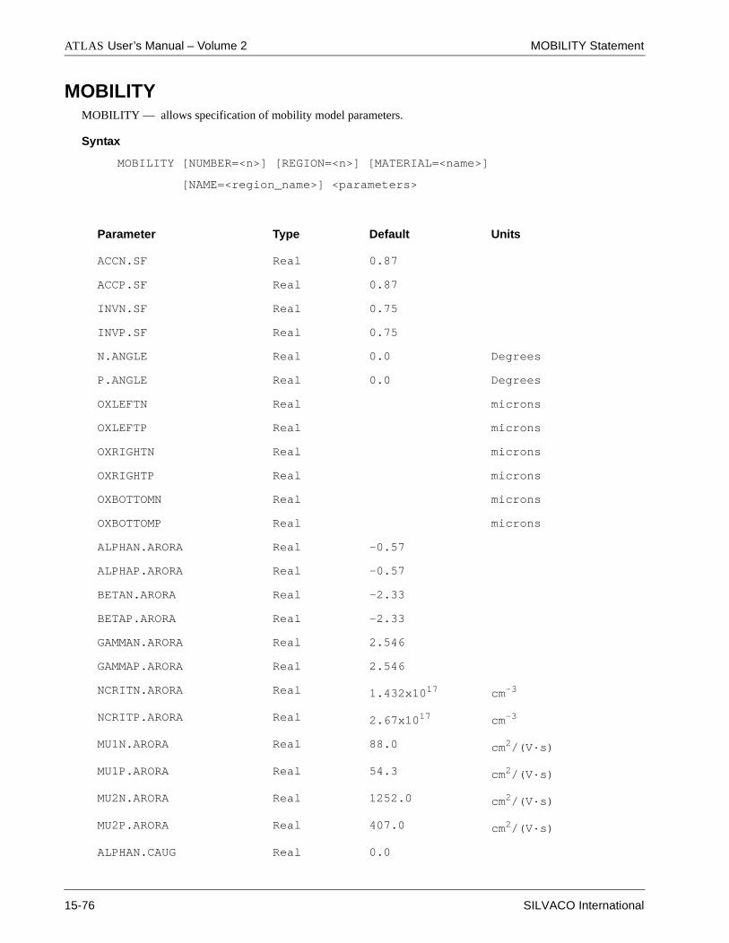
ATLAS User’s Manual – Volume 2 MOBILITY Statement
MOBILITYMOBILITY — allows specification of mobility model parameters.
Syntax
MOBILITY [NUMBER=<n>] [REGION=<n>] [MATERIAL=<name>]
[NAME=<region_name>] <parameters>
Parameter Type Default Units
ACCN.SF Real 0.87
ACCP.SF Real 0.87
INVN.SF Real 0.75
INVP.SF Real 0.75
N.ANGLE Real 0.0 Degrees
P.ANGLE Real 0.0 Degrees
OXLEFTN Real microns
OXLEFTP Real microns
OXRIGHTN Real microns
OXRIGHTP Real microns
OXBOTTOMN Real microns
OXBOTTOMP Real microns
ALPHAN.ARORA Real -0.57
ALPHAP.ARORA Real -0.57
BETAN.ARORA Real -2.33
BETAP.ARORA Real -2.33
GAMMAN.ARORA Real 2.546
GAMMAP.ARORA Real 2.546
NCRITN.ARORA Real 1.432x1017 cm-3
NCRITP.ARORA Real 2.67x1017 cm-3
MU1N.ARORA Real 88.0 cm2/(V·s)
MU1P.ARORA Real 54.3 cm2/(V·s)
MU2N.ARORA Real 1252.0 cm2/(V·s)
MU2P.ARORA Real 407.0 cm2/(V·s)
ALPHAN.CAUG Real 0.0
15-76 SILVACO International

MOBILITY Statement Statements
ALPHAP.CAUG Real 0.0
BETAN.CAUG Real -2.3
BETAP.CAUG Real -2.2
DELTAN.CAUG Real 0.73
DELTAP.CAUG Real 0.70
GAMMAN.CAUG Real -3.8
GAMMAP.CAUG Real -3.7
NCRITN.CAUG Real 1.072x1017 cm-3
NCRITP.CAUG Real 1.606x1017 cm-3
MU1N.CAUG Real 55.24 cm2/(V·s)
MU1P.CAUG Real 49.7 cm2/(V·s)
MU2N.CAUG Real 1429.23 cm2/(V·s)
MU2P.CAUG Real 479.37 cm2/(V·s)
AL1N.WATT Real -0.16
AL1P.WATT Real -0.296
AL2N.WATT Real -2.17
AL2P.WATT Real -1.62
AL3N.WATT Real 1.07
AL3P.WATT Real 1.02
ETAN.WATT Real 0.50
ETAP.WATT Real 0.33
MREF1N.WATT Real 481.0 cm2/(V·s)
MREF1P.WATT Real 92.8 cm2/(V·s)
MREF2N.WATT Real 591.0 cm2/(V·s)
MREF2P.WATT Real 124.0 cm2/(V·s)
MREF3N.WATT Real 1270.0 cm2/(V·s)
MREF3P.WATT Real 534.0 cm2/(V·s)
MOD.WATT.N Logical False
MOD.WATT.P Logical False
EXP.WATT.N Logical False
Parameter Type Default Units
SILVACO International 15-77
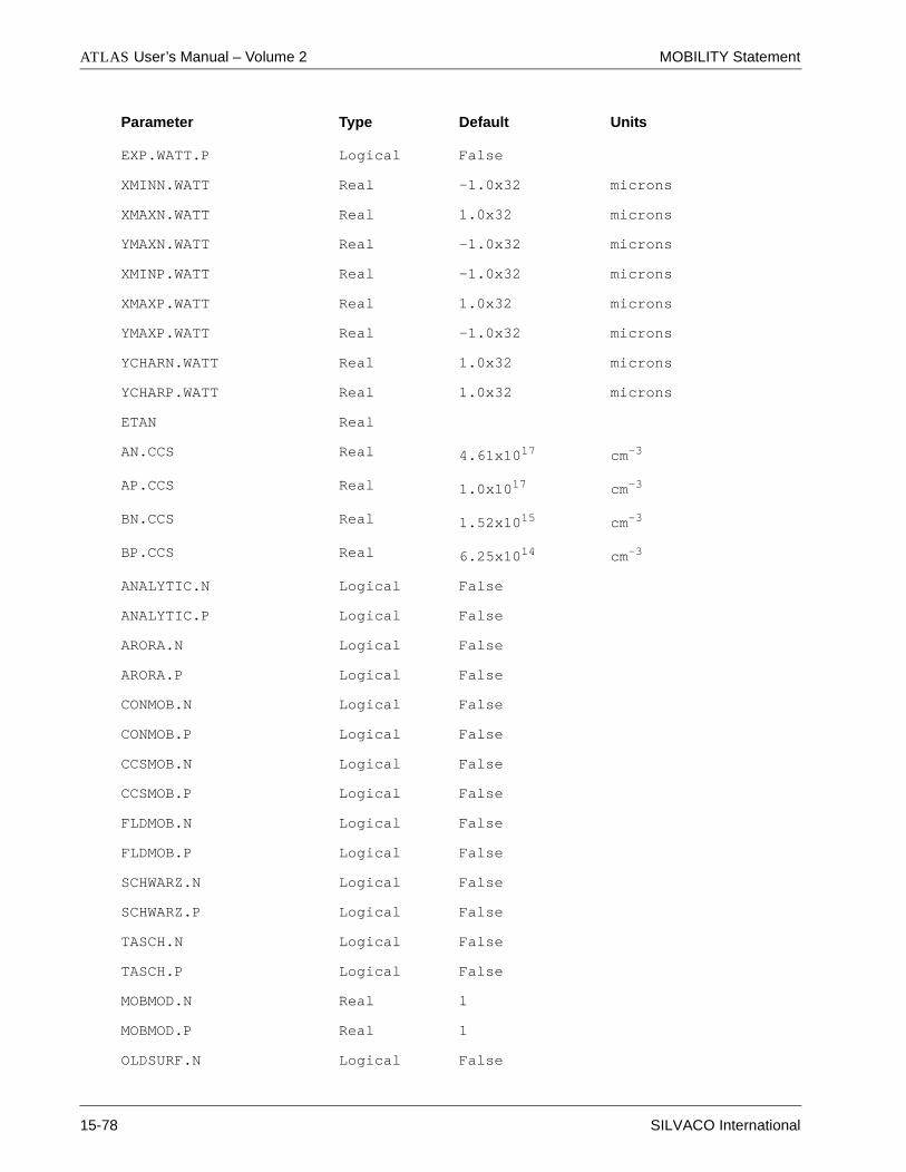
ATLAS User’s Manual – Volume 2 MOBILITY Statement
EXP.WATT.P Logical False
XMINN.WATT Real -1.0x32 microns
XMAXN.WATT Real 1.0x32 microns
YMAXN.WATT Real -1.0x32 microns
XMINP.WATT Real -1.0x32 microns
XMAXP.WATT Real 1.0x32 microns
YMAXP.WATT Real -1.0x32 microns
YCHARN.WATT Real 1.0x32 microns
YCHARP.WATT Real 1.0x32 microns
ETAN Real
AN.CCS Real 4.61x1017 cm-3
AP.CCS Real 1.0x1017 cm-3
BN.CCS Real 1.52x1015 cm-3
BP.CCS Real 6.25x1014 cm-3
ANALYTIC.N Logical False
ANALYTIC.P Logical False
ARORA.N Logical False
ARORA.P Logical False
CONMOB.N Logical False
CONMOB.P Logical False
CCSMOB.N Logical False
CCSMOB.P Logical False
FLDMOB.N Logical False
FLDMOB.P Logical False
SCHWARZ.N Logical False
SCHWARZ.P Logical False
TASCH.N Logical False
TASCH.P Logical False
MOBMOD.N Real 1
MOBMOD.P Real 1
OLDSURF.N Logical False
Parameter Type Default Units
15-78 SILVACO International

MOBILITY Statement Statements
OLDSURF.P Logical False
SURFMOB.N Logical False
SURFMOB.P Logical False
ASN.YAMA Real 1.54x10⁻⁵ cm/V
ASP.YAMA Real 5.35x10⁻⁵ cm/V
GN.YAMA Real 8.8 cm/s
GP.YAMA Real 1.6 cm/s
NREFN.YAMA Real 3.0x1016 cm-3
NREFP.YAMA Real 4.0x1016 cm-3
MULN.YAMA Real 1400.0 cm2/(V·s)
MULP.YAMA Real 480.0 cm2/(V·s)
SN.YAMA Real 350
SP.YAMA Real 81.0
VSN.YAMA Real 1.036x10 7 cm/s
VSP.YAMA Real 1.200x10 7 cm/s
ULN.YAMA Real 4.9x10 6 cm/s
ULP.YAMA Real 2.928x10 6 cm/s
ALPHN.CVT Real 0.680
ALPHP.CVT Real 0.71
BN.CVT Real 4.75x10 7 cm/(K·s)
BP.CVT Real 9.925x10 6 cm/(K·s)
BETAN.CVT Real 2.00
BETAP.CVT Real 2.00
CN.CVT Real 1.74x10 5
CP.CVT Real 8.842x10 5
CRN.CVT Real 9.68x10 16 cm-3
CRP.CVT Real 2.23x10 17 cm-3
CSN.CVT Real 3.43x10 20 cm-3
CSP.CVT Real 6.10x10 20 cm-3
Parameter Type Default Units
SILVACO International 15-79

ATLAS User’s Manual – Volume 2 MOBILITY Statement
DELN.CVT Real 5.82x10¹⁴ V/s
DELP.CVT Real 2.0546x10¹⁴ V/s
GAMN.CVT Real 2.5
GAMP.CVT Real 2.2
MU0N.CVT Real 52.2 cm2/(V·s)
MU0P.CVT Real 44.9 cm2/(V·s)
MU1N.CVT Real 43.4 cm2/(V·s)
MU1P.CVT Real 29.0 cm2/(V·s)
MUMAXN.CVT Real 1417.0 cm2/(V·s)
MUMAXP.CVT Real 470.5 cm2/(V·s)
PCN.CVT Real 0.0 cm-3
PCP.CVT Real 0.23x10 16 cm-3
TAUN.CVT Real 0.125
TAUP.CVT Real 0.0317
DEVICE Character
MATERIAL Character
NAME Character
ECRITN Real 4.0x10 3 V/cm
ECRITP Real 4.0x10 3 V/cm
GAMMAN Real 4.0
GAMMAP Real 1.0
RN.TAS Real 2
RP.TAS Real 3
MUBN.TAS Real 1150
MUBP.TAS Real 270
TMUBN.TAS Real 2.5
TMUBP.TAS Real 1.4
DN.TAS Real 3.2x10 -9
DP.TAS Real 2.35x10 -9
P1N.TAS Real 0.09
Parameter Type Default Units
15-80 SILVACO International

MOBILITY Statement Statements
P1P.TAS Real 0.334
B1N.TAS Real 1.75
B1P.TAS Real 1.5
P2N.TAS Real 4.53x10⁻⁸
P2P.TAS Real 3.14x10⁻⁷
B2N.TAS Real -0.25
B2P.TAS Real -0.3
Z11N.TAS Real 0.0388
Z11P.TAS Real 0.039
Z22N.TAS Real 1.73x10⁻⁵
Z22P.TAS Real 1.51x10⁻⁵
ESRN.TAS Real 2.449x10⁷
ESRP.TAS Real 1.0x10⁹
BETAN.TAS Real 2
BETAP.TAS Real 1
N2N.TAS Real 1.1x10²¹
N2P.TAS Real 1.4x10¹⁸
N1N.TAS Real 2.0x10¹⁹
N1P.TAS Real 8.4x10¹⁶
ALPHAN.TAS Real 2
ALPHAP.TAS Real 3.4
BETAN Real 2.0
BETAP Real 1.0
VSATN Real cm/s
VSATP Real cm/s
ALPHAN.FLD Real 2.4x107 cm/s
ALPHAP.FLD Real 2.4x107 cm/s
THETAN.FLD Real 0.8
THETAP.FLD Real 0.8
TNOMN.FLD Real 600.0 K
Parameter Type Default Units
SILVACO International 15-81

ATLAS User’s Manual – Volume 2 MOBILITY Statement
TNOMP.FLD Real 600.0 K
EVSATMOD Real 0
HVSATMOD Real 0
F.CONMUN Character
F.CONMUP Character
F.MUNSAT Character
F.MUPSAT Character
F.VSATN Character
F.VSATP Character
MUDEG.N Real 1.0
MUDEG.P Real 1.0
MUN Real 1.0 cm2/(V·s)
MUP Real 1.0 cm2/(V·s)
TMUP Real 1.0
TMUN Real 1.0
KLA.N Logical False
KLA.P Logical False
SHI.N Logical False
SHI.P Logical False
MUMAXN.KLA Real 1417.0 cm2/(V·s)
MUMAXP.KLA Real 470.5.0 cm2/(V·s)
MUMINN.KLA Real 52.2 cm2/(V·s)
MUMINP.KLA Real 44.9 cm2/(V·s)
NREF1N.KLA Real 9.68x16 cm-3
NREF1P.KLA Real 2.23x17 cm-3
ALPHA1N.KLA Real 0.68
ALPHA1P.KLA Real 0.719
THETAN.KLA Real 2.285
THETAP.KLA Real 2.247
CD.KLA Real 0.21
CA.KLA Real 0.50
Parameter Type Default Units
15-82 SILVACO International

MOBILITY Statement Statements
NREFD.KLA Real 4.0x20 cm-3
NREFA.KLA Real 7.2x20 cm-3
FCW.KLA Real 2.459
FBH.KLA Real 3.828
S1.KLA Real 0.89233
S2.KLA Real 0.41372
S3.KLA Real 0.19778
S4.KLA Real 0.28227
S5.KLA Real 0.005978
S6.KLA Real 1.80618
S7.KLA Real 0.72169
R1.KLA Real 0.7643
R2.KLA Real 2.2999
R3.KLA Real 6.5502
R4.KLA Real 2.3670
R5.KLA Real -0.8552
R6.KLA Real 0.6478
MU0N.SHI Real 1430.0 cm2/(V·s)
MU0P.SHI Real 500.0 cm2/(V·s)
E1N.SHI Real 6.3e3 V/cm
E1P.SHI Real 8.0e3 V/cm
E2N.SHI Real 0.77e6 V/cm
E2P.SHI Real 3.9e5 V/cm
P1N.SHI Real 0.28
P1P.SHI Real 0.3
P2N.SHI Real 2.9
P2P.SHI Real 1.0
THETAN.SHI Real 2.285
THETAP.SHI Real 2.247
Parameter Type Default Units
SILVACO International 15-83

ATLAS User’s Manual – Volume 2 MOBILITY Statement
Description
MATERIAL specifies which material from the table B-1 that the MOBILITY statement should apply to. If a materialis specified, then all regions defined as being composed of that material will be affected.
DEVICE specifies the device in MIXEDMODE simulation that the MOBILITY statement should apply to.
NAME specifies the name of the region that the MOBILITY statement should apply. Note that the name must matchthe name specified in the NAME parameter of the REGION statement.
Mobility Model Flags
N.ANGLE specifies angle for application of electron mobility parameters in simulation of anisotropic mobility..
P.ANGLE specifies angle for application of hole mobility parameters in simulation of anisotropic mobility.
FLDMOB.N specifies a lateral electric field dependent model for electrons (see Equation 3-198).
FLDMOB.P specifies a lateral electric field dependent model for holes (see Equation 3-199).
CONMOB.N specifies that doping concentration dependent model to be used for electrons.
CONMOB.P specifies that a doping concentration dependent model is to be used for holes.
CCSMOB.N specifies that carrier-carrier scattering model is to be used for electrons (see Equations 3-128 - 3-131).
CCSMOB.P specifies that carrier-carrier scattering model is to be used for holes (see Equations 3-128 - 3-131).
ANALYTIC.N specifies that the analytic concentration dependent model is to be used for electrons (see Equation 3-124).
ANALYTIC.P specifies that the analytic concentration dependent model is to be used for holes (see Equation 3-125).
ARORA.N specifies that the Arora analytic concentration dependent model is to be used for electrons (see Equation3-126).
ARORA.P specifies that the Arora analytic concentration dependent model is to be used for electrons (see Equation 3-127).
SURFMOB.N invokes the effective field based surface mobility model for electrons (see Equation 3-190).
SURFMOB.P invokes the effective field based surface mobility model for holes (see Equation 3-191).
SCHWARZ.N specifies the use of transverse electric field-dependent mobility models for electrons. See TFLDMB1 orSCHWARZ in the MODELS statement.
SCHWARZ.P specifies the use of transverse electric field-dependent mobility models for holes. See TFLDMB1 orSCHWARZ in the MODELS statement.
TASCH.N specifies a transverse electric field dependent mobility model for electrons based on Tasch7,9 (seeEquations 3-171 through 3-189).
TASCH.P specifies a transverse electric field dependent mobility model for holes based on Tasch7,9 (see Equations3-171 through 3-189).
EVSATMOD specifies which parallel field dependent mobility model (see Equations 3-198 and 5-50) should be usedfor electrons as follows:
1. Use the standard saturation model (Equation 3-198).
2. Use the negative differential mobility saturation model (Equation 5-50).
MOBMOD.N specifies transverse field degradation for electrons as follows:
1. No transverse degradation.
2. Use the Watt or Tasch transverse field models depending on the settings of FIELDMOB1 and FIELDMOB2.
3. Use the Yamaguchi transverse field dependent model.
15-84 SILVACO International

MOBILITY Statement Statements
4. Use the CVT transverse field dependent model.
MOBMOD.P specifies transverse field degradation for electrons as follows:
1. No transverse degradation.
2. Use the Watt or Tasch transverse field models depending on the settings of FIELDMOB1 and FIELDMOB2.
3. Use the Yamaguchi transverse field dependent model.
4. Use the CVT transverse field dependent model.
KLA.N turns on Klaassen’s mobility model for electrons (see Equations 3-132 through 3-157.
KLA.P turns on Klaassen’s mobility model for holes (see Equations 3-132 through 3-157).
MOD.WATT.N turns on modified Watt mobility model for electrons (see page 3-194).
MOD.WATT.Pturns on modified Watt mobility model for holes (see page 3-195).
EXP.WATT.N turns on exponertial modification to Watt’s mobility model for electrons (see Equation 3-194).
EXP.WATT.P turns on exponential modification to Watt’s mobility model for holes (see Equation 3-195).
SHI.N turns on Shirahata’s mobility model for electrons (see Equation 3-196).
SHI.P turns on Shirahata’s mobility model for holes (see Equation 3-197)
Temperature Dependent Low Field Mobility Parameters
MUN see Table 3-16.
MUP see Table 3-16.
TMUN see Table 3-16.
TMUP see Table 3-16.
Arora Concentration Dependent Mobility Model Parameters
MU1N.ARORA see Table 3-19.
MU1P.ARORA see Table 3-19.
MU2N.ARORA see Table 3-19.
MU2P.ARORA see Table 3-19.
ALPHAN.ARORA see Table 3-19.
ALPHAP.ARORA see Table 3-19.
BETAN.ARORA see Table 3-19.
BETAP.ARORA see Table 3-19.
GAMMAN.ARORA see Table 3-19.
GAMMAP.ARORA see Table 3-19.
NCRITN.ARORA see Table 3-19.
NCRITP.ARORA see Table 3-19.
Caughey-Thomas Concentration Dependent Model Parameters
MU1N.CAUG see Table 3-18.
MU1P.CAUG see Table 3-18.
MU2N.CAUG see Table 3-18.
SILVACO International 15-85

ATLAS User’s Manual – Volume 2 MOBILITY Statement
MU2P.CAUG see Table 3-18.
ALPHAN.CAUG see Table 3-18.
ALPHAP.CAUG see Table 3-18.
BETAN.CAUG see Table 3-18.
BETAP.CAUG see Table 3-18.
GAMMAN.CAUG see Table 3-18.
GAMMAP.CAUG see Table 3-18.
DELTAN.CAUG see Table 3-18.
DELTAP.CAUG see Table 3-18.
NCRITN.CAUG see Table 3-18.
NCRITP.CAUG see Table 3-18.
Carrier-Carrier Scattering Model Parameters
AN.CCS see Table 3-20.
AP.CCS see Table 3-20.
BN.CCS see Table 3-20
BP.CCS see Table 3-20.
Parallel Field Dependent Model Parameters
BETAN see Table 3-33.
BETAP see Table 3-33.
GAMMAN see Table 5-3.
GAMMAP see Table 5-3.
ECRITN see Table 5-3.
ECRITP see Table 5-3.
VSATN see Tables 3-33 and 5-3.
VSATP see Tables 3-33 and 5-3.
ALPHAN.FLD see Table 3-33.
ALPHAP.FLD see Table 3-33.
THETAN.FLD see Table 3-33.
THETAP.FLD see Table 3-33.
TNOMN.FLD see Table 3-33.
TNOMP.FLD see Table 3-33.
Yamaguchi Transverse Field Dependent Model Parameters
SN.YAMA see Table 3-29.
SP.YAMA see Table 3-29.
NREFN.YAMA see Table 3-29.
NREFP.YAMA see Table 3-29.
15-86 SILVACO International

MOBILITY Statement Statements
MULN.YAMA see Table 3-29.
MULP.YAMA see Table3-29.
ASN.YAMA see Table 3-29.
ASP.YAMA see Table 3-29.
VSN.YAMA see Table 3-29.
VSP.YAMA see Table 3-29.
ULN.YAMA see Table 3-29.
ULP.YAMA see Table 3-29.
GN.YAMA see Table3-29.
GP.YAMA see Table 3-29.
CVT Transverse Field Dependent Model Parameters
BN.CVT see Table 3-28
BP.CVT see Table 3-28
CN.CVT see Table 3-28
CP.CVT see Table 3-28
TAUN.CVT see Table 3-28.
TAUP.CVT see Table 3-28.
GAMN.CVT see Table 3-28.
GAMP.CVT see Table 3-28.
MU0N.CVT see Table 3-28.
MU0P.CVT see Table3-28.
MU1N.CVT see Table 3-28..
MU1P.CVT see Table 3-28.
MUMAXN.CVT see Table 3-28.
MUMAXP.CVT see Table 3-28.
CRN.CVT see Table 3-28.
CRP.CVT see Table 3-28.
CSN.CVT see Table 3-28.
CSP.CVT see Table 3-28.
ALPHN.CVT see Table 3-28.
ALPHP.CVT see Table 3-28.
BETAN.CVT see Table 3-28.
BETAP.CVT see Table 3-28.
PCN.CVT see Table 3-28.
PCP.CVT see Table 3-28.
DELN.CVT see Table 3-28.
DELP.CVT see Table 3-28.
SILVACO International 15-87

ATLAS User’s Manual – Volume 2 MOBILITY Statement
Watt Effective Transverse Field Depenedent Model Parameters
ETAN.WATT see Table 3-31
ETAP.WATT see Table 3-31
MREF1N.WATT 3-31.
MREF1P.WATT 3-31.
MREF2N.WATT see Table 3-31.
MREF2P.WATT see Table3-31.
MREF3N.WATT see Table 3-31.
MREF3P.WATT see Table 3-31.
AL1N.WATT see Table 3-31.
AL1P.WATT see Table 3-31.
AL2N.WATT see Table 3-31.
AL2P.WATT see Table 3-31.
AL3N.WATT see Table 3-31.
AL3P.WATT see Table 3-31
Tasch Mobility Model Parameters
RN.TAS see Table 3-30
RP.TAS see Table 3-30
MUBN.TAS see Table 3-30
MUBP.TAS see Table 3-30
TMUBN.TAS see Table 3-30
TMUBP.TAS see Table 3-30
DN.TAS see Table 3-30
DP.TAS see Table 3-30
P1N.TAS see Table 3-30
P1P.TAS see Table 3-30
B1N.TAS see Table 3-30
B1P.TAS see Table 3-30
P2N.TAS see Table 3-30
P2P.TAS see Table 3-30
B2N.TAS see Table 3-30
B2P.TAS see Table 3-30
Z11N.TAS see Table 3-30
Z11P.TAS see Table 3-30
Z22N.TAS see Table 3-30
Z22P.TAS see Table 3-30
ESRN.TAS see Table 3-30
15-88 SILVACO International

MOBILITY Statement Statements
ESRP.TAS see Table 3-30
BETAN.TAS see Table 3-30
BETAP.TAS see Table 3-30
N2N.TAS see Table 3-30
N2P.TAS see Table 3-30
N1N.TAS see Table 3-30
N1P.TAS see Table 3-30
ALPHAN.TAS see Table 3-30
ALPHAP.TAS see Table 3-30
Klaassen’s Mobility Model Parameters
MUMAXN.KLA see Table 3-21.
MUMAXP.KLA see Table 3-21
MUMINN.KLA see Table 3-23.
MUMINP.KLA see Table 3-23.
NREF1N.KLA see Table 3-22.
NREF1P.KLA see Table 3-22.
ALPHA1N.KLA see Table 3-22.
ALPHA1P.KLA see Table 3-22.
THETAN.KLA see Table 3-21
THETAP.KLA see Table 3-21
CD.KLA see Table 3-27
CA.KLA see Table 3-27.
NREFD.KLA see Table 3-27
NREFA.KLA see Table 3-27
FCW.KLA see Table 3-26.
FBH.KLA see Table 3-26.
S1.KLA see Table 3-24.
S2.KLA see Table 3-24.
S3.KLA see Table 3-24.
S4.KLA see Table 3-24.
S5.KLA see Table 3-24.
S6.KLA see Table 3-24.
S7.KLA see Table 3-24.
R1.KLA see Table 3-25.
R2.KLA see Table 3-25.
R3.KLA see Table 3-25.
SILVACO International 15-89

ATLAS User’s Manual – Volume 2 MOBILITY Statement
R4.KLA see Table 3-25.
R5.KLA see Table 3-25.
R6.KLA see Table 3-25.
The Modified Watt Mobility Model Parameters
XMINN.WATT see pege 3-52.
XMAXN.WATT see page 3-52.
YMAXN.WATT see page 3-52.
XMINP.WATT see page 3-52.
XMAXP.WATT see page 3-52.
YMAXP.WATT see page 3-52.
YCHARN.WATT see page 3-52.
YCHARP.WATT see page 3-52.
Shirahata’s Mobility Model Parameters
MU0N.SHI see Table 3-32.
MU0P.SHI see Table 3-32.
E1N.SHI see Table 3-32.
E1P.SHI see Table 3-32.
E2N.SHI see Table 3-32.
E2P.SHI see Table 3-32.
P1N.SHI see Table 3-32.
P1P.SHI see Table 3-32.
P2N.SHI see Table 3-32.
P2P.SHI see Table 3-32.
THETAN.SHI see Table 3-32.
THETAP.SHI see Table 3-32.
SCHWARZ and TASCH Transverse Field Dependent Model Parameters
ACCN.SF specifies the accumulation saturation factor which describes the ratio of the electron concentration in theaccumulation layer before and after bending of conductivity and valence bands for electron mobility.
ACCN.SF specifies the accumulation saturation factor which describes the ratio of the hole concentration in theaccumulation layer before and after bending of conductivity and valence bands for hole mobility.
INVN.SF specifies the inversion saturation factor which describes the ratio of the electron concentration in theinversion layer before and after the bending of conductivity and valence bands for electron mobility.
INVN.SF specifies the inversion saturation factor which describes the ratio of the hole concentration in the inversionlayer before and after the bending of conductivity and valence bands for hole mobility.
OXBOTTOMN specifies the coordinate of the bottom edge of the gate oxide for a MOSFET transistor for electronmobility.
15-90 SILVACO International

MOBILITY Statement Statements
OXBOTTOMP specifies the coordinate of the bottom edge of the gate oxide for a MOSFET transistor for holemobility.
OXLEFTN specifies the coordinate of the left edge of the gate oxide for a MOSFET transistor for electron mobility.
OXLEFTP specifies the coordinate of the left edge of the gate oxide for a MOSFET transistor for hole mobility.
OXRIGHTN specifies the coordinate of the right edge of the gate oxide for a MOSFET transistor for electronmobility.
OXRIGHTP specifies the coordinate of the right edge of the gate oxide for a MOSFET transistor for hole mobility.
Interpreter Functions
F.CONMUN specifies the name of a file containing a C-INTERPRETER function for the specification of temperature,composition and doping dependent electron mobility model.
F.CONMUP specifies the name of a file containing a C-INTERPRETER function for the specification of temperature,composition and doping dependent hole mobility model.
F.MUNSAT specifies the name of a file containing a C-INTERPRETER function for the specification of parallel fielddependent electron mobility model for velocity saturation.
F.MUPSAT specifies the name of a file containing a C-INTERPRETER function for the specification of parallel fielddependent hole mobility model for velocity saturation.
F.VSATN specifies the name of a file containing a C-INTERPRETER function for the specification of temperature andcomposition dependent electron saturation velocity models.
F.VSATP specifies the name of a file containing a C-INTERPRETER function for the specification of temperature andcomposition dependent electron saturation velocity models.
Example Selecting the Modifed Watt Model
The following example set the Modified Watt Surface mobility model for MOSFETs. This is the best model for planarMOS simulation. The MOBILITY statement is used to set the models and to specify the value of the depth of action ofthe Modified Watt model.
MODELS CONMOB FLDMOB SRH MIN.SURF PRINT
MOBILITY WATT.N MOD.WATT.N YMAXN.WATT=0.01
SILVACO International 15-91
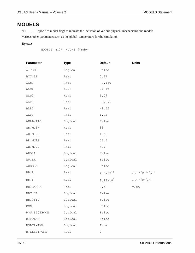
ATLAS User’s Manual – Volume 2 MODELS Statement
MODELSMODELS — specifies model flags to indicate the inclusion of various physical mechanisms and models.
Various other parameters such as the global temperature for the simulation.
Syntax
MODELS <mf> [<gp>] [<mdp>
Parameter Type Default Units
A.TEMP Logical False
ACC.SF Real 0.87
ALN1 Real -0.160
ALN2 Real -2.17
ALN3 Real 1.07
ALP1 Real -0.296
ALP2 Real -1.62
ALP3 Real 1.02
ANALYTIC Logical False
AR.MU1N Real 88
AR.MU2N Real 1252
AR.MU1P Real 54.3
AR.MU2P Real 407
ARORA Logical False
AUGER Logical False
AUGGEN Logical False
BB.A Real 4.0x1014 cm-1/2V-5/2s-1
BB.B Real 1.97x107 cm-1/2V-2s-1
BB.GAMMA Real 2.5 V/cm
BBT.KL Logical False
BBT.STD Logical False
BGN Logical False
BGN.SLOTBOOM Logical False
BIPOLAR Logical False
BOLTZMANN Logical True
B.ELECTRONS Real 2
15-92 SILVACO International

MODELS Statement Statements
B.HOLES Real 1
C0 Real 2.5x10⁻¹⁰
CALC.FERMI Logical False
CAVITY.LENGTH Real µm
CCS.EA Real 4.61x10¹⁷
CCS.EB Real 1.52x10¹⁵
CCS.HA Real 1.0x10¹⁷
CCS.HB Real 6.25x10¹⁴
CCSMOB Logical False
CGATE.N Real 0.025
CGATE.P Real 150.0
CHIA Real 3e5
CHIB Real 5.0x10⁴
CHI.HOLES Real 4.6x10⁴
CONMOB Logical False
CONSRH Logical False
CVT Logical False
B.DORT Real 1.0
D.DORT Real 2.5x10⁶
N.DORT Logical False
P.DORT Logical False
DEVDEG.E Logical False
DEVDEG.H Logical False
DEVDEG.B Logical False
DEVICE Character
DRIFT.DIFF Logical True
E.BENDING Logical False
E.TAUR.VAR Logical False
ECRIT Real 4000.0 V/cm
EIGENS Integer 15
ENERGY.STEP Real 0.0025 eV
Parameter Type Default Units
SILVACO International 15-93
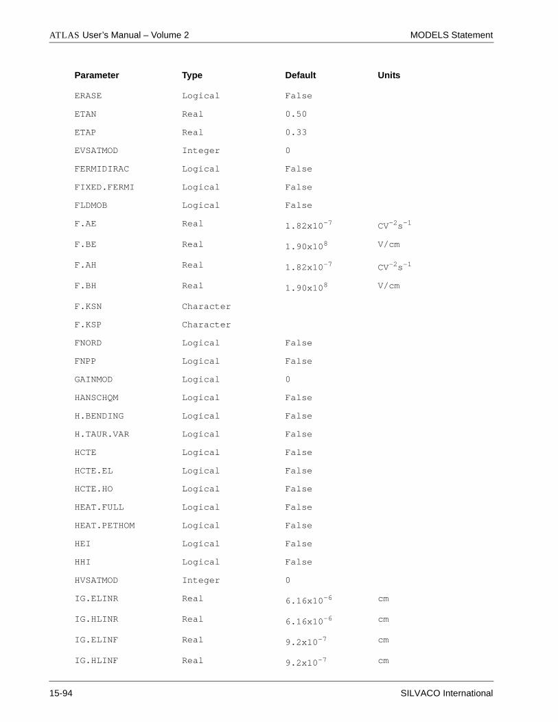
ATLAS User’s Manual – Volume 2 MODELS Statement
ERASE Logical False
ETAN Real 0.50
ETAP Real 0.33
EVSATMOD Integer 0
FERMIDIRAC Logical False
FIXED.FERMI Logical False
FLDMOB Logical False
F.AE Real 1.82x10⁻⁷ CV-2s-1
F.BE Real 1.90x10⁸ V/cm
F.AH Real 1.82x10⁻⁷ CV-2s-1
F.BH Real 1.90x10⁸ V/cm
F.KSN Character
F.KSP Character
FNORD Logical False
FNPP Logical False
GAINMOD Logical 0
HANSCHQM Logical False
H.BENDING Logical False
H.TAUR.VAR Logical False
HCTE Logical False
HCTE.EL Logical False
HCTE.HO Logical False
HEAT.FULL Logical False
HEAT.PETHOM Logical False
HEI Logical False
HHI Logical False
HVSATMOD Integer 0
IG.ELINR Real 6.16x10⁻⁶ cm
IG.HLINR Real 6.16x10⁻⁶ cm
IG.ELINF Real 9.2x10⁻⁷ cm
IG.HLINF Real 9.2x10⁻⁷ cm
Parameter Type Default Units
15-94 SILVACO International

MODELS Statement Statements
IG.EBETA Real 2.59x10⁻⁴ (V.cm)0.5
IG.HBETA Real 2.59x10⁻⁴ (V.cm)0.5
IG.EETA Real 2.0x10⁻⁵ V1/3.cm2/3
IG.HETA Real 2.0x10⁻⁵ V1/3.cm2/3
IG.EEOX Real 9.0x10⁴ V/cm
IG.HEOX Real 9.0x10⁴ V/cm
IG.EB0 Real 3.2 V
IG.HB0 Real 4.0 V
IMPACT Logical False
INCOMPLETE Logical False
INFINITY Real 0.001
IONIZ Logical False
INV.SF Real 0.75
KSN Integer 0-1
KSP Integer 0-1
KLA Logical False
KAUGDP Real 0.72
L.TEMP Logical False
LAT.TEMP Logical False
LASER Logical False
LMODE Logical False
LAS.ABSORPTION Logical False
LAS.EINIT Real eV
LAS.ESEP Real eV
LAS.EFINAL Real eV
LAS.FCARRIER Logical False
LAS.ITMAX Integer 30
LAS.LOSSES Real 0 cm-1
LAS.MAXCH Real 2.5
LAS.MIRROR Real 90 %
LAS.MULTISAVE Logical False
Parameter Type Default Units
SILVACO International 15-95

ATLAS User’s Manual – Volume 2 MODELS Statement
LAS.NEFF Real 3.57
LAS.OMEGA Real 2.16x10¹⁵ 1/sec
LAS.SIN Real 1.0x104 cm-1
LAS.SPECSAVE Integer 1
LAS.TAUSS Real 0.05
LAS.TIMERATE Logical True
LAS.TOLER Real 0.001
MATERIAL Character
MIN.SURF Logical False
MOBMOD Integer
MOS Logical False
MREFN1 Real 481.0 cm2/Vs
MREFN2 Real 591.0 cm2/Vs
MREFN3 Real 1270.0 cm2/Vs
MREFP1 Real 92.8 cm2/Vs
MREFP2 Real 124. cm2/Vs
MREFP3 Real 534. cm2/Vs
N.CONCANNON Logical False
N.TEMP Logical False
NAME Character
NEARFLG Logical False
OPTR Logical False
OX.LEFT Real mm
OX.RIGHT Real µm
OX.BOTTOM Real 0.0 µm
P.CONCANNON Logical False
P.TEMP Logical False
PATH.N Real 3.4x10⁷ microns
PATH.P Real 2.38x10⁻⁷ microns
PEFF.N Real 3.2 eV
Parameter Type Default Units
15-96 SILVACO International
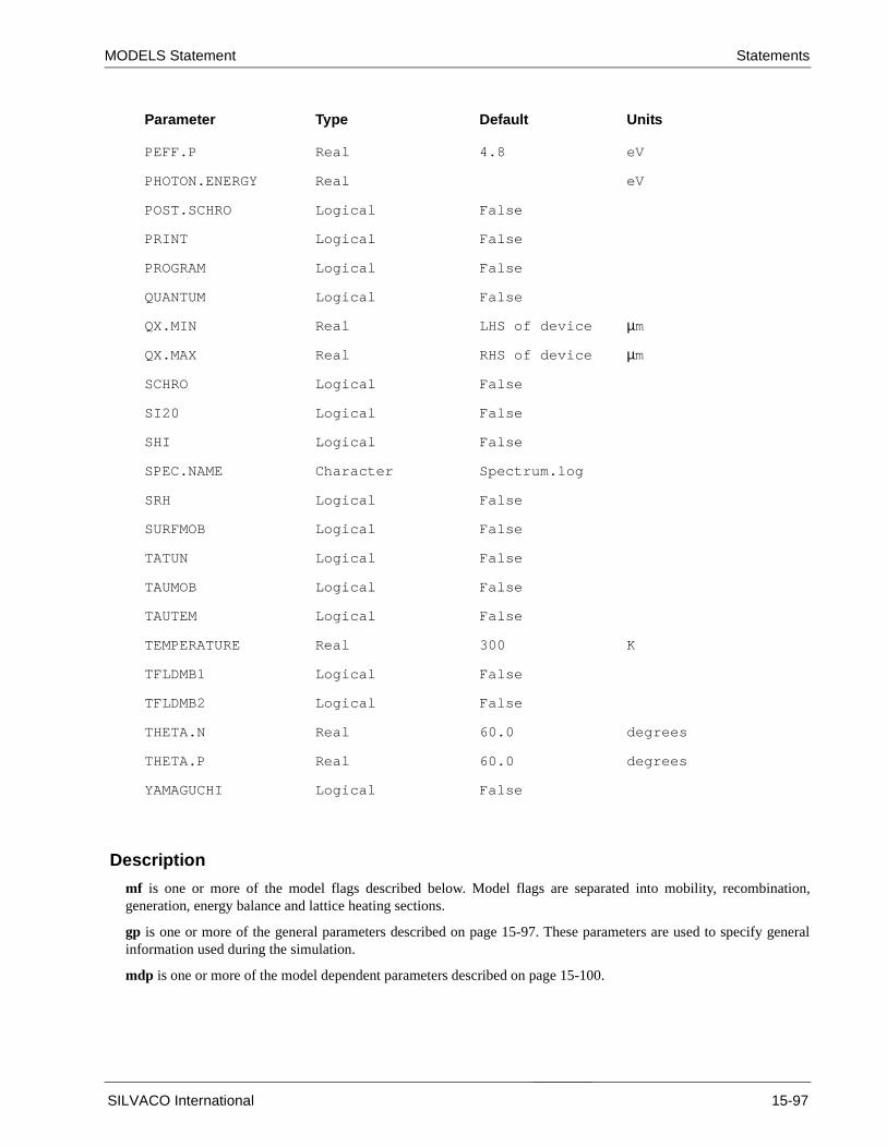
MODELS Statement Statements
Description
mf is one or more of the model flags described below. Model flags are separated into mobility, recombination,generation, energy balance and lattice heating sections.
gp is one or more of the general parameters described on page 15-97. These parameters are used to specify generalinformation used during the simulation.
mdp is one or more of the model dependent parameters described on page 15-100.
PEFF.P Real 4.8 eV
PHOTON.ENERGY Real eV
POST.SCHRO Logical False
PRINT Logical False
PROGRAM Logical False
QUANTUM Logical False
QX.MIN Real LHS of device µm
QX.MAX Real RHS of device µm
SCHRO Logical False
SI20 Logical False
SHI Logical False
SPEC.NAME Character Spectrum.log
SRH Logical False
SURFMOB Logical False
TATUN Logical False
TAUMOB Logical False
TAUTEM Logical False
TEMPERATURE Real 300 K
TFLDMB1 Logical False
TFLDMB2 Logical False
THETA.N Real 60.0 degrees
THETA.P Real 60.0 degrees
YAMAGUCHI Logical False
Parameter Type Default Units
SILVACO International 15-97

ATLAS User’s Manual – Volume 2 MODELS Statement
ion.
e
Mobility Model Flags
Note: See the MOBILITY statement for alternative ways to set mobility models
ANALYTIC specifies an analytic concentration dependent mobility model for silicon which includes temperaturedependence (see Equations 3-124 and 3-125).
ARORA specifies an analytic concentration and temperature dependent model according to Arora (see Equations 3-126 and 3-127).
CCSMOB specifies carrier-carrier scattering model according to Dorkel and Leturq (see Equation 3-128- 3-131).
CONMOB specifies that a concentration dependent mobility model be used for silicon and gallium arsenide. Thismodel is a doping versus mobility table valid for 300K only.
CVT specifies that the CVT transverse field dependent mobility model is used for the simulation.
FLDMOB specifies a lateral electric field-dependent model (see Equations 3-198 and 5-50). The EVSATMODparameter may be used to define which field dependent equation is used..
KLA specifies that the Klaassen mobility model (See Equations 3-132 - 3-157) will be used for electrons and holes.
MIN.SURF specifies that the WATT, TASCH, or SHI mobility models should only apply to minority carriers.
MOBMOD specifies mobility degradation by longitudinal electric field only (MOBMOD=1), or by both longitudinaland transverse electric fields (MOBMOD=2). When MOBMOD=2, the parameters ACC.SF, INV.SF, OX.BOTTOM,OX.LEFT, and OX.RIGHT.This parameter is only used with TFLDMB1 and TFLDMB2
SHI specifies that the Shirahata mobility model (See Equation 3-197) will be used for electrons and holes.
SURFMOB or WATT invokes the effective field based surface mobility model (see Equations 3-190 and 3-191).
SURFMOB parameters are used in the calculation of surface mobility according to the J.T. Watt model5. Do not specifythis parameter unless S-PISCES is installed on your system.
TFLDMB1 or SCHWARZ specifies the use of transverse electric field-dependent mobility models. The electronmodel is based on the Schwarz and Russek equations [6] and is implemented in [7]. The hole model, which is used
only when MOBMOD=2, is based on the Watt and Plummer equations8.
TFLDMB2 or TASCH specifies a transverse electric field dependent mobility model for electrons and holes basedon a semi-empirical equation [7,9].
YAMAGUCHI specifies that the Yamaguchi transverse field dependent mobility model is used in the simulation.
Recombination Model Flags
AUGER specifies Auger recombination (see Equation 3-227)
AUGGEN specifies that the Auger recombination model will be used as a generation term as well as a recombinationterm.
CONSRH Specifies Shockley-Read-Hall recombination using concentration dependent lifetimes (see Equations 3-215 and 3-216).
KLAAUG enables Klaassen’s model for concentration dependent auger coefficients.
KLASRH enables Klaassen’s model for concentration dependent lifetimes for Shockley Read Hall recombinat
OPTR selects the optical recombination model (see Equation 3-226). When this parameter is specified, thCOPTparameter of the MATERIAL statement should be specified.
SRH specifies Shockley-Read-Hall recombination using fixed lifetimes (see Equation 3-213).
TATUN enables the Klaassen trap-assisted tunneling model.
15-98 SILVACO International

MODELS Statement Statements
nd 3-
Generation Model Flags
BBT.KL specifies a band-to-band tunneling model according to Klaassen.
BBT.STD specifies a standard band-to-band tunneling model (see Equation 3-270).
DEVDEG.E activates the device degradation caused by hot electron injection current. HEI should also be specified inthis case.
DEVDEG.H activates the device degradation caused by hot hole injection current. HHI should also be specified inthis case.
DEVDEG.B activates the device degradation caused by both the hot electron and hot hole injection currents. HEI andHHI should also be specified in this case.
Note: The specification of either DEVDEG.E, DEVDEG.H, or DEVDEG.B will initialize the density ofelectron (hole) like traps on the interface and will clear out the trapped electron (hole) density on theinterface if any.
E.BENDING specifies that electron band bending will be taken into account for electron injection (see Equation 3-279).
FNORD selects a self-consistent Fowler-Nordheim tunneling model (see Equation 3-274).This is the recommendedapproach for calculating Fowler-Nordheim current.
FNPP selects a post-processing Fowler-Nordheim tunneling model (see Equation 3-275). Generally the Fowler-Nordheim current does not cause convergence problems so this appraoch is not required.
H.BENDING specifies that hole band bending will be taken into account for hole injection (see Equation 3-282).
HEI specifies the calculation of hot electron injection into oxides. This parameter can be used to simulate MOS gatecurrent or EPROM programming. In transient mode, the oxide current is self-consistently added to the floating gatecharge. See Equation 3-277.
HHI specifies the calculation of hot hole current into an oxide in a similar manner to HEI (see Equation 3-278).
IMPACT invokes the empirical impact ionization model with ionization coefficients taken from 12. More rigorousimpact ionization models may be specified with the IMPACT statement.
NEARFLG specifies the model used for oxide transport when HEI or HHI are used. The default is false which sets apurely drift based model assigning gate current to the electrodes where the electric field lines through the oxideterminate. Setting NEARFLG replaces this model with one assuming the gate current is flowing the electrodephysically nearest the point of injection. This assumes a purely diffusion transport mechanism.Setting NEARFLG fordevices with only one gate or a coarse mesh is advised.
N.CONCANNON enables the Concannon gate current model for electrons.
P.CONCANNON enables the Concannon gate current model for holes.
Classical Carrier Statistics Model Flags
BGN specifies band-gap narrowing (see Equation 3-38).
BGN.SLOTBOOM specifies band-gap narrowing using the original Slotboom coefficients (see Equation 3-38).
BOLTZMANN specifies that Boltzmann carrier statistics be used (see Equations 3-25 and 3-26).
FERMIDIRAC specifies that Fermi-Dirac carrier statistics be used (see Equations 3-25 – 3-62).
INCOMPLETE accounts for incomplete ionization of impurities in Fermi-Dirac statistics (see Equations 3-43 a44).
IONIZ accounts for complete ionization of heavily doped silicon when using INCOMPLETE.
SILVACO International 15-99

ATLAS User’s Manual – Volume 2 MODELS Statement
Quantum Carrier Statistics Model Flags
EIGENS specifies the number of eigenstates solved for by the Poisson-Schrodinger solver.
CALC.FERMI specifies that the Fermi level used in calculation of the quantum carrier concentration in theSchrodinger - Poisson model is calculated from the classic carrier concentrations.
FIXED.FERMI specifies that a constant Fermi level is used along each individual slice in the Y direction for carrierconcentration calculation in the Schrodinger - Poisson model.
HANSCHQM turns on the Hansch quantum effects approximation model for N channel MOS devices.
POST.SCHRO specifies to calculate the Schrodinger equation for quantum effects as a post processing step.
SCHRO enables the Poisson-Schrodinger solver. This can be used for zero carrier solutions only (specified byMETHOD CARRIERS=0). This is typically combined with the EIGENS parameter to control the number ofeigenstates calculated. This is a 1D solver that is solved within the mesh between limits set by QX.MIN and QX.MAX.
N.DORT turns on the Van Dort quantum effects approximation model for N channel MOS devices.
P.DORT turns on the Van Dort quantum effects approximation model for P channel MOS devices.
QUANTUM enables the quantum moments model.
QX.MIN, QX.MAX specify the minimum and maximum extent of the Poisson-Schrodinger solver along the x-axisdirection.
Energy Balance Simulation Flags
E.TAUR.VAR specifies that electron temperature dependent energy relaxation time is used. Use parametersTRE.T1, TRE.T2, TRE.T3, TRE.W1, TRE.W2 and TRE.W3 on material statement to specifie the energyrelaxation time.
H.TAUR.VAR specifies that hole temperature dependent energy relaxation time is used. Use parameters TRH.T1,TRH.T2, TRH.T3, TRH.W1, TRH.W2 and TRH.W3 on material statement to specifie the energy relaxationtime.
HCTE specifies that both electron and hole temperature will be solved.
HCTE.EL specifies that electron temperature will be solved.
HCTE.HO specifies that hole temperature will be solved.
F.KSN specifies the name of a file containing a C-INTERPRETER function specifying the electron Peltier coefficientas a function of electron energy.
F.KSP specifies the name of a file containing a C-INTERPRETER function specifying the hole Peltier coefficient as afunction of hole energy.
KSN specifies which hot carrier transport model will be used for electrons. KSN=0 selects the hydrodynamic modeland KSN=-1 selects the energy balance model.
KSP specifies which hot carrier transport model will be used for holes. KSP=0 selects the hydrodynamic model andKSP=-1 selects the energy balance model.
TAUMOB specifies the dependence of relaxation times with carrier temperature in the mobility definition. IfTAUMOB is specified, the values of MATERIAL statement parameters TAUMOB.EL and TAUMOB.HO are dependenton the carrier temperature.
TAUTEM specifies the dependence of relaxation times with carrier temperature. If TAUTEM is specified, the values ofMATERIAL statement parameters TAUREL.EL and TAUREL.HO are dependent on carrier temperature..
N.TEMP or HCTE.EL specifies that the electron temperature equation will be solved.
P.TEMP or HCTE.HO specifies that the hole temperature equation will be solved.
15-100 SILVACO International
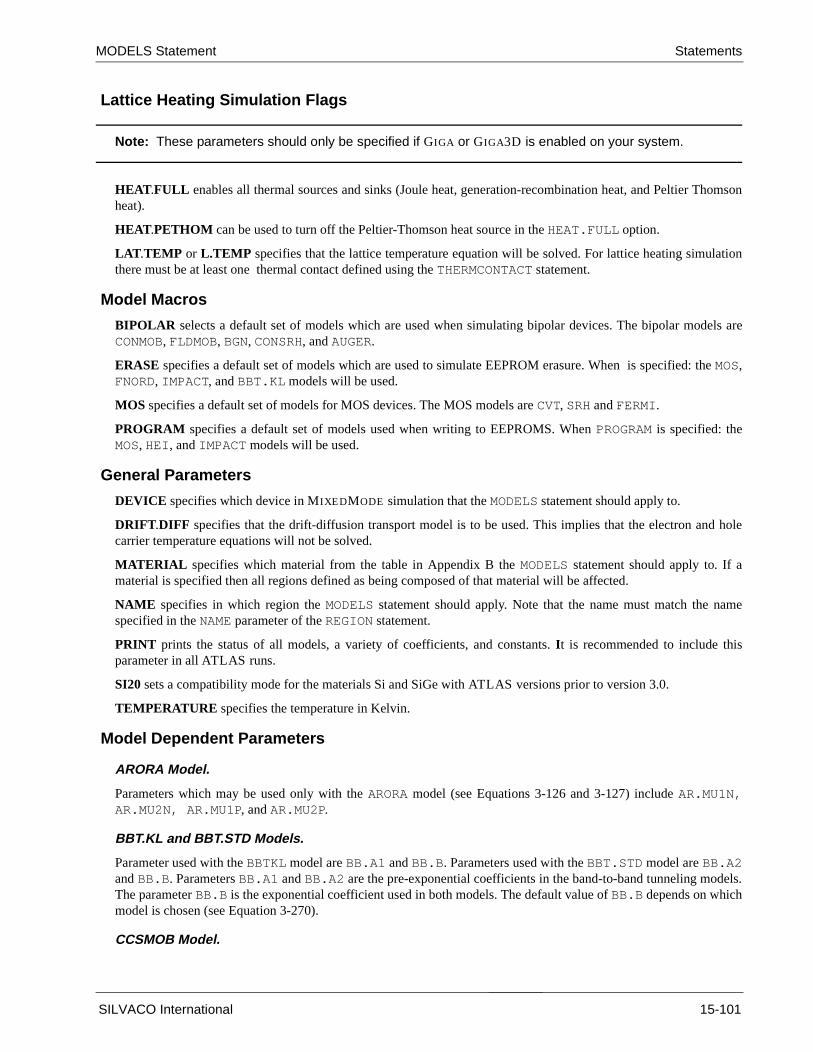
MODELS Statement Statements
Lattice Heating Simulation Flags
Note: These parameters should only be specified if GIGA or GIGA3D is enabled on your system.
HEAT.FULL enables all thermal sources and sinks (Joule heat, generation-recombination heat, and Peltier Thomsonheat).
HEAT.PETHOM can be used to turn off the Peltier-Thomson heat source in the HEAT.FULL option.
LAT.TEMP or L.TEMP specifies that the lattice temperature equation will be solved. For lattice heating simulationthere must be at least one thermal contact defined using the THERMCONTACT statement.
Model Macros
BIPOLAR selects a default set of models which are used when simulating bipolar devices. The bipolar models areCONMOB, FLDMOB, BGN, CONSRH, and AUGER.
ERASE specifies a default set of models which are used to simulate EEPROM erasure. When is specified: the MOS,FNORD, IMPACT, and BBT.KL models will be used.
MOS specifies a default set of models for MOS devices. The MOS models are CVT, SRH and FERMI.
PROGRAM specifies a default set of models used when writing to EEPROMS. When PROGRAM is specified: theMOS, HEI, and IMPACT models will be used.
General Parameters
DEVICE specifies which device in MIXEDMODE simulation that the MODELS statement should apply to.
DRIFT.DIFF specifies that the drift-diffusion transport model is to be used. This implies that the electron and holecarrier temperature equations will not be solved.
MATERIAL specifies which material from the table in Appendix B the MODELS statement should apply to. If amaterial is specified then all regions defined as being composed of that material will be affected.
NAME specifies in which region the MODELS statement should apply. Note that the name must match the namespecified in the NAME parameter of the REGION statement.
PRINT prints the status of all models, a variety of coefficients, and constants. It is recommended to include thisparameter in all ATLAS runs.
SI20 sets a compatibility mode for the materials Si and SiGe with ATLAS versions prior to version 3.0.
TEMPERATURE specifies the temperature in Kelvin.
Model Dependent Parameters
ARORA Model.
Parameters which may be used only with the ARORA model (see Equations 3-126 and 3-127) include AR.MU1N,AR.MU2N, AR.MU1P, and AR.MU2P.
BBT.KL and BBT.STD Models.
Parameter used with the BBTKL model are BB.A1 and BB.B. Parameters used with the BBT.STD model are BB.A2and BB.B. Parameters BB.A1 and BB.A2 are the pre-exponential coefficients in the band-to-band tunneling models.The parameter BB.B is the exponential coefficient used in both models. The default value of BB.B depends on whichmodel is chosen (see Equation 3-270).
CCSMOB Model.
SILVACO International 15-101

ATLAS User’s Manual – Volume 2 MODELS Statement
e used
e used
tion in
in the
The parameters CCS.EA, CCS.EB, CCS.HA, and CCS.HB describe the dependendence of mobility on doping,carrier concentration, and temperature. See Equations 3-128 – 3-131.
FLDMOB Model.
B.ELECTRONS is used in the field-dependent mobility expression for EVSATMOD=0 (see Equation 3-198).
B.HOLES is used in the field-dependent mobility expression for EVSATMOD=0 (see Equation 3-199).
E0 is used in the field dependent mobility model for EVSATMOD=1 (see Equation 5-50).
EVSATMOD specifies which parallel field dependent mobility model (see Equations 3-198 and 5-50) should bfor electrons as follows:
0. Use the standard saturation model
1. Use the negative differtial velocity saturation model
2 Use a simple velocity limiting model.
In most cases the default value of 0 should be used.
HVSATMOD specifies which parallel field dependent mobility model (see Equations 3-199 and 5-51) should bfor holes as follows:
0. Use the standard saturation model
2 Use a simple velocity limiting model.
In most cases the default value of 0 should be used.
Fowler-Nordheim Tunneling Model.
Parameters used in this model are F.AE and F.BE. F.AE is the pre-exponential factor and F.BE is theexponenential coefficient (see Equation 3-274).
WATT or SURFMOB Model.
The parameters which may be used with the WATT model include ALN1, ALN2, ALN3, ALP1, ALP2,ALP3, ETAN, ETAP, MREFN1, MREFN2, MREFN3, MREFP1, MREFP2, and MREFP3 (see Equations3-190 and 3-191).
TFLDMB1 and TFLDMB2 Models.
ACC.SF specifies the accumulation saturation factor which describes the ratio of the majority carrier concentrathe accumulation layer before and after bending of conductivity and valence bands.
INV.SF specifies the inversion saturation factor which describes the ratio of the majority carrier concentrationinversion layer before and after the bending of conductivity and valance bands.
OX.BOTTOM specifies the coordinate of the bottom edge of the gate oxide for a MOSFET transistor.
OX.LEFT specifies the coordinate of the left edge of the gate oxide for a MOSFET transistor.
OX.RIGHT specifies the coordinate of the right edge of the gate oxide for a MOSFET transistor.
CONCANNON Model Parameters
CGATE.N specifies an empirical tuning factor for electrons in the Concannon gate current model.
CGATE.P specifies an empirical tuning factor for holes in the Concannon gate current model.
PEFF.N specifies an effective barrier height for electrons in the Concannon gate current model.
PEFF.P specifies an effective barrier height for holes in the Concannon gate current model.
15-102 SILVACO International

MODELS Statement Statements
-3).
Rapid
ctivity )
THETA.N specifies the critical rejection angle for electrons in the Concannon gate current model.
THETA.P specifies the critical rejection angle for electrons in the Concannon gate current model.
C0 specifies the electron distribution weight factor in the Concannon gate current model.
CHIA specifies the electron distribution function constant in the Concannon gate current model.
CHIB specifies the electron distribution function constant in the Concannon gate current model.
CHI.HOLES specifies the hole distribution function constant in the Concannon gate current model.
ENERGY.STEP specifies the energy step for numeric integration in the Concannon gate current model.
INFINITY specifies the highest energy in numeric integration in the Concannon gate current model.
PATH.N specifies the mean free path in the oxide for electrons in the Concannon gate current model.
PATH.P specifies the mean free path in the oxide for holes in the Concannon gate current model.
HEI Model Parameters
The parameters which may be used with the HEI model include IG.ELINR, IG.HLINR, IG.ELINF, IG.HLINF,IG.EBETA, IG.HBETA, IG.EETA, IG.HETA, IG.EEOX, IG.HEOX, IG.EB0, IG.HB0.
N.DORT and P.DORT Model parameters
B.DORT user specifiable model parameter for the van Dort quantum effects approximation model.
D.DORT user specifiable model parameter for the van Dort quantum effects approximation model.
LASER Simulation Parameters
CAVITY.LENGTH specifies the cavity length in the longitudinal direction (in µm).
GAINMOD specifies the local optical gain model to be used.
• GAINMOD=0 specifies that no optical gain model will be used.
• GAINMOD=1 specifies that the complex frequency-dependent gain model will be used (see Equation 9
• GAINMOD=2 specifies that the simple gain model will be used (see Equation 9-6).
LASER enables LASER simulation.
LMODE specifies that multiple longitudinal models are to be taken into account during LASERT
simulation.
LAS.ABSORPTION enables the absorption loss model in LASER.
LAS.EINIT, LAS.EFINAL specify the lower and upper photon energies. LASER will calculate multiple longitudinalphoton rates within this range. Using wide ranges can slow down simulation.
LAS.ESEP specifies the photon energy separation. If this is not specified, LASER will automatically calculate thenumber of longitudinal modes based on the cavity length and the energy range.
LAS.FCARRIER enables the free carrier loss model in LASER.
LAS.ITMAX specifies the maximum number of iterations allowed for LASER simulation at each bias point.
LAS.LOSSES specifies the total losses in Equation 9-8.
LAS.MAXCH specifies the maximum allowable relative charge in photon densities between iterations. changes of the photon densities can cause convergence problems.
LAS.MIRROR specifies the percentage facet reflectivity ( both facets are assumed to have this value of reflefor the mirror loss in Laser. 100 % reflectivity is equalivent to no mirror loss.
SILVACO International 15-103

ATLAS User’s Manual – Volume 2 MODELS Statement
LAS.MULTISAVE specifies the whether or not to save the transient LASER spectrum as one file or multiple files.
LAS.NEFF specifies the effective refractive index in Equation 9-2.
LAS.OMEGA specifies the lasing frequency to be used in Equation 9-1. If model 2 is used for simulation, then thisparameter specifies an estimate of the lasting frequency. Instead of using this parameter, PHOTON.ENERGY can beused to specify photon energy.
LAS.SIN specifies an initial photon density in the fundamental lasing mode. This value provides an initial guess forsubsequent iterations. This parameter is used only when the single frequency model has been selected.
LAS.SPECSAVE the spectrum file will be saved after every LAS.SPECSAVE LASER solution steps.
LAS.TAUSS specifies the iteration parameter to be used for the photon rate equation when solving Equation 9-8.
LAS.TIMERATE specifies that the time dependent photon rate equation will be used in a transient laser simulation.
LAS.TOLER specifies the desired accuracy in photon areas.
PHOTON.ENERGY specifies the energy of photons. If model 2 is used for simulation, this parameter specifies onlyan initial estimate of the photon energy. Instead of using this parameter, LAS.OMEGA can be used to specify the lasingfrequency.
SPEC.NAME specifies the name of a spectrum file, which LASER will produce for each bias point if the LMODESparameter has been specified.
Model Selection Example
This example selects concentration and field dependent mobilities, SRH recombination, and Auger recombination.This is a typical model set for bipolar simulation. The simulation temperature is 290K.
MODELS CONMOB FLDMOB SRH AUGER TEMP=290
Confirming Model Selection
To echo back model selections, parameters and material constants use
MODELS PRINT
Note: For the best MODEL selection for different applications, consult the Standard Example set.
15-104 SILVACO International

OPTIONS Statement Statements
lly used,
OPTIONSOPTIONS — sets options for an entire run.
Syntax
OPTIONS [<rcp>]
Description
rcp is one or more of the run control parameters described below. These parameters, which are not normaspecify debugging options.
NORMAL is the default specification for run-time output filtering. At this setting ATLAS prints out the mostrelevant information (e.g. mesh statistics, terminal voltages, currents, warnings and error messages).
QUIET specifies the maximum of filtering of run-time output.
VERBOSE specifies the mimimum filtering of run-time output. You should specify VERBOSE if you want output ofresidual norms.
Example
The following syntax can be used to provide extra debugging output.
OPTION VERBOSE
Note: The VERBOSE output is of little interest to most users
Parameter Type Default Units
NORMAL Logical True
QUIET Logical False
VERBOSE Logical False
SILVACO International 15-105

ATLAS User’s Manual – Volume 2 OUTPUT Statement
OUTPUTOUTPUT — allows the user to specify the data that will be stored in standard structure format files.
Syntax
OUTPUT <parameters>
Parameter Type Default Units
ANGLE Logical False
AREA Logical False
BAND.PARAM Logical False
CHARGE Logical False
CON.BAND Logical False
CONTACT Integer
DELTAV Real 0.1 Volts
DEVDEG Logical False
E.FIELD Logical False
E.LINES Logical False
E.MOBILITY Logical False
E.TEMP Logical True
E.VELOCITY Logical False
EFIELD Logical False
EIGENS Integer 7
EX.FIELD Logical True
EX.VELOCITY Logical False
EY.FIELD Logical True
EY.VELOCITY Logical False
FLOWLINES Logical False
H.MOBILITY Logical False
H.TEMP Logical True
H.VELOCITY Logical False
HX.VELOCITY Logical False
HY.VELOCITY Logical False
IMPACT Logical True
INV.AREA Logical False
INV.ANGLE Logical True
15-106 SILVACO International

OUTPUT Statement Statements
INAME Character
JX.ELECTRON Logical False
J.ELECTRON Logical True
JX.ELECTRON Logical False
J.CONDUC Logical True
J.DISP Logical False
J.HOLE Logical True
J.TOTAL Logical True
JX.CONDUC Logical False
JX.HOLE Logical False
JX.TOTAL Logical False
JY.CONDUC Logical False
JY.HOLE Logical False
JY.TOTAL Logical False
KSN Logical False
KSP Logical False
LRATIO Real 1.0
MINSET Logical False
N.LINES Integer
OPT.INTENS Logical False
OX.CHARGE Logical False
OLD.AVG Logical False
PERMITTIVITY Logical False
PHOTOGEN Logical True
QFN Logical True
QFP Logical True
QSS Logical False
RECOMB Logical True
TAURN Logical False
TAURP Logical False
TOT.DOPING Logical False
TRAPS Logical True
Parameter Type Default Units
SILVACO International 15-107
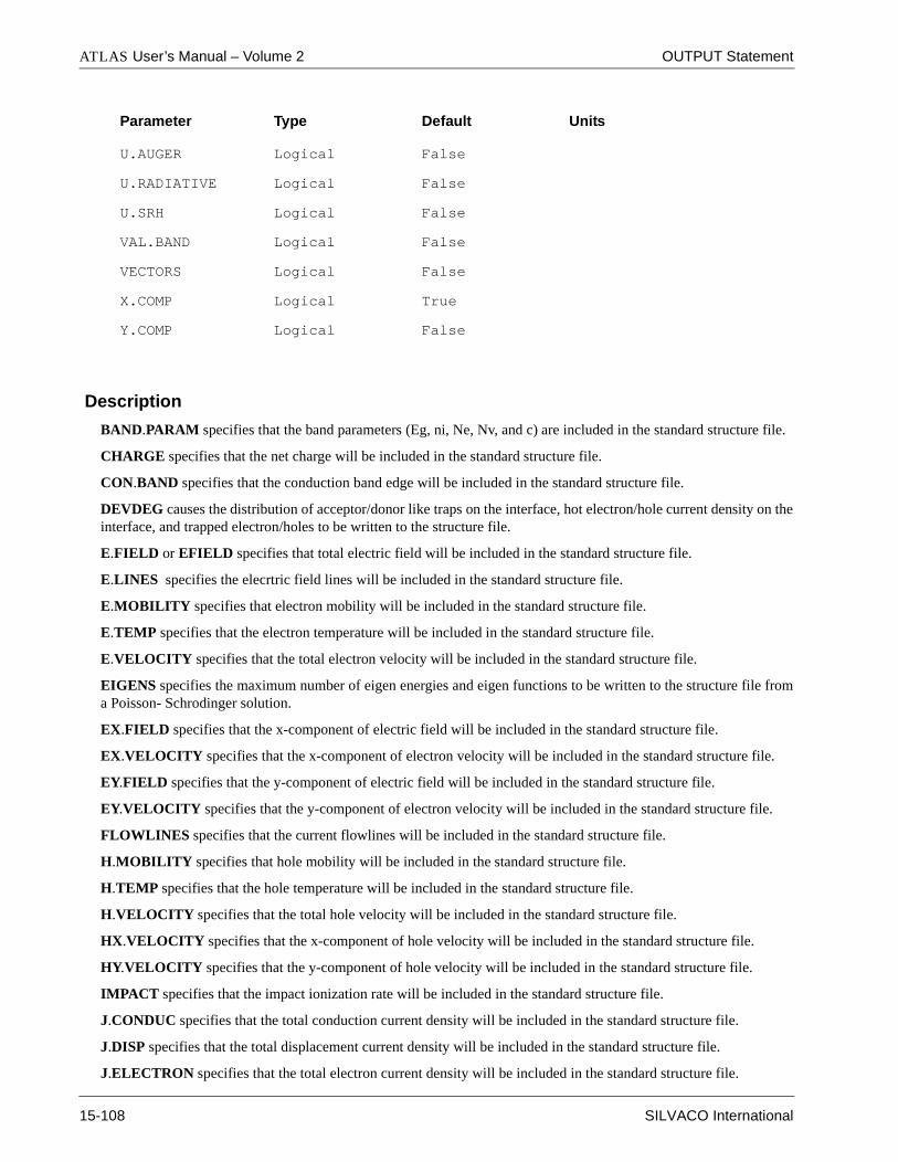
ATLAS User’s Manual – Volume 2 OUTPUT Statement
Description
BAND.PARAM specifies that the band parameters (Eg, ni, Ne, Nv, and c) are included in the standard structure file.
CHARGE specifies that the net charge will be included in the standard structure file.
CON.BAND specifies that the conduction band edge will be included in the standard structure file.
DEVDEG causes the distribution of acceptor/donor like traps on the interface, hot electron/hole current density on theinterface, and trapped electron/holes to be written to the structure file.
E.FIELD or EFIELD specifies that total electric field will be included in the standard structure file.
E.LINES specifies the elecrtric field lines will be included in the standard structure file.
E.MOBILITY specifies that electron mobility will be included in the standard structure file.
E.TEMP specifies that the electron temperature will be included in the standard structure file.
E.VELOCITY specifies that the total electron velocity will be included in the standard structure file.
EIGENS specifies the maximum number of eigen energies and eigen functions to be written to the structure file froma Poisson- Schrodinger solution.
EX.FIELD specifies that the x-component of electric field will be included in the standard structure file.
EX.VELOCITY specifies that the x-component of electron velocity will be included in the standard structure file.
EY.FIELD specifies that the y-component of electric field will be included in the standard structure file.
EY.VELOCITY specifies that the y-component of electron velocity will be included in the standard structure file.
FLOWLINES specifies that the current flowlines will be included in the standard structure file.
H.MOBILITY specifies that hole mobility will be included in the standard structure file.
H.TEMP specifies that the hole temperature will be included in the standard structure file.
H.VELOCITY specifies that the total hole velocity will be included in the standard structure file.
HX.VELOCITY specifies that the x-component of hole velocity will be included in the standard structure file.
HY.VELOCITY specifies that the y-component of hole velocity will be included in the standard structure file.
IMPACT specifies that the impact ionization rate will be included in the standard structure file.
J.CONDUC specifies that the total conduction current density will be included in the standard structure file.
J.DISP specifies that the total displacement current density will be included in the standard structure file.
J.ELECTRON specifies that the total electron current density will be included in the standard structure file.
U.AUGER Logical False
U.RADIATIVE Logical False
U.SRH Logical False
VAL.BAND Logical False
VECTORS Logical False
X.COMP Logical True
Y.COMP Logical False
Parameter Type Default Units
15-108 SILVACO International

OUTPUT Statement Statements
J.HOLE specifies that the total hole current density will be included in the standard structure file.
J.TOTAL specifies that the total current density will be included in the standard structure file.
JX.CONDUC specifies that the x-component of the total conduction current density will be included in the standardstructure file.
JX.ELECTRON specifies that the x-component of electron current density will be included in the standard structurefile.
JX.HOLE specifies that the x-component of hole current density will be included in the standard structure file.
JX.TOTAL specifies that the x-component of total current density will be included in the standard structure file.
JY.CONDUC specifies that the y-component of the total conduction current density will be included in the standardstructure file.
JY.ELECTRON specifies that the y-component of electron current density will be included in the standard structurefile.
JY.HOLE specifies that the y-component of hole current density will be included in the standard structure file.
JY.TOTAL specifies that the y-component of total current density will be included in the standard structure file.
KSN specifies that electron Peltier coefficients are to be written to any saved structure file.
KSP specifies that hole Peltier coefficients are to be written to any saved structure file.
MINSET that a minimum set of data (potential, carrier concentration, and electric field) will be included in thestandard structure file.
OPT.INTENS specifies that optical intensity is included in the standard structure file.
OX.CHARGE specifies that fixed oxide charge is inclued in the standard structure file.
PERMITTIVITY specifies the dielectric permittivity is saved
PHOTOGEN specifies that the photogeneration rate will be included in the standard structure file.
QFN specifies that the electron quasi-fermi level will be included in the standard structure file.
QFP specifies that the hole quasi-fermi level will be included in the standard structure file.
QSS specifies that the surface charge will be included in the standard structure file.
RECOMB specifies that the recombination rate will be included in the standard structure file.
TAURN specifies that electron relaxation times are to be written to any saved structure file.
TAURP specifies that hole relaxation times are to be written to any saved structure file.
TOT.DOPING specifies that total doping will be included in the standard structure file.
TRAPS specifies that trap density information will be included in the standard structure file.
U.AUGER specifies that the Auger component of recombination is to be written to solution files.
U.RADIATIVE specifies that the radiative component of recombination is to be written to solution files.
U.SRH specifies that the SRH component of recombination is to be written to solution files.
VAL.BAND specifies that the valence band edge will be included in the standard structure file.
VECTORS specifies that only vector components will be included in the standard structure file.
X.COMP specifies that the composition fraction “x” is to be written to solution files.
Y.COMP specifies that the composition fraction “y” is to be written to solution files.
SILVACO International 15-109

ATLAS User’s Manual – Volume 2 OUTPUT Statement
Ionization Integral Parameters
Note: See the SOLVE statement and the on-line examples for instructions on using ionization integrals
INAME specifies the name of a contact for which electric field lines are calculated.
CONTACT specifies a contact number for which electric field lines are calculated.
LRATIO specifies the spacing ratio between adjacent electric field lines. Defaults to 1.0 for uniform spacing.
N.LINES specifies the number of electric field lines.
DELTAV since the electric field is near zero at the contact, the electric field line calculations begin at a distance fromthe contact at which the contact voltage has changed by DELTAV. Defaults to 0.1 V.
Averaging Parameters for Vector Quantities
OLD.AVG specifies that the current and field quantities will be averaged using an older algorithm (from version3.0.0.R and back). By default the new method is used.
ANGLE specifies that averaging of current and fields will be weighted by the size of the angle of trianglesintersecting at the node.
INV.ANGLE specifies that averaging of current and fields will be weighted by the inverse of the size of the angle oftriangles intersecting at the node.
AREA specifies that averaging of current and fields will be weighted by the areas of triangles intersecting at the node.
INV.AREA specifies that averaging of current and fields will be weighted by the inverse of areas of trianglesintersecting at the node.
Note: Certain quantities that can be output into the structure file and subsequently displayed usingTONYPLOT need special mention. These quantities are evaluated within ATLAS along the links betweengrid points. They are represented in the structure file at the grid points themselves. As such thesequantities are subject to averaging. In particular, electric field and currents are averaged so as to takeinto account the vector nature of these values. Mobility is simply summed up over all the linkssurrounding the grid point and divided by the total number of links. Carrier velocities are derived bydividing the averaged current by the carrier density at the grid point and the fundamental electron chargeq.
Example of combining OUTPUT with SOLVE and SAVE
The OUTPUT statement is often used in conjuction with the SAVE statement. The following statement lines specifythat current flowlines and electron velocity components are saved in all subsequent standard structure solution files.
OUTPUT FLOWLINES EX.VELO EY.VELO
SOLVE PREVIOUS V5=2 OUTF=data1.str MASTER
SAVE OUTF=data2.str
15-110 SILVACO International

PROBE Statement Statements
ny ofe LOG
PROBEPROBE — allows users to output the minimum value, maximum value or value at a specified location of aseveral distributed quantities to the LOG file. The quantities will be saved at each bias point of timestep in thfile.
Note: PROBE is the most accurate way to determine the value of many parameters calculated byATLAS. Parameters stored on node points in the structure files for Tonyplot are often interpolated andsubject to noise.
Syntax
PROBE[MIN|MAX|X=<n>Y=<n>[DIR=<n>]][POTENTIAL|N.CONC|P.CONC|N.TEMP|P.TEMP|LAT.TEMP|GENERATION|RECOMBINATION|RSRH|RAUGER|RRADIATIVE]
Parameter Type Default Units
DEVICE Character
DIR Real 0.0 degrees
FIELD Logical False
LAT.TEMP Logical False
MAX Logical False
MIN Logical False
N.CONC Logical False
N.MOB Logical False
N.TEMP Logical False
NAME Character
P.CONC Logical False
P.MOB Logical False
P.TEMP Logical False
POLARIZATION Logical False
POTENTIAL Logical False
QFN Logical False
QFP Logical False
RAUGER Logical False
RECOMBIN Logical False
RRADIATIVE Logical False
SILVACO International 15-111

ATLAS User’s Manual – Volume 2 PROBE Statement
Description
DEVICE specifies which device in mixed mode simulation the probe statement should apply to.
DIR specifies the direction relative to the x axis in degrees associated with certain directed quantities. Thesequantities include FIELD, N.MOB, P.MOB and POLARIZATION.
Note: The algorithm used finds the triangle in the mesh containing the specified X and Y values. Thenthe value of the DIR parameter is used to find which edge of the triangle lies in the direction nearest thatvalue
FIELD - specifies that a value of electric field is probed. The DIR parameter should also be specified if FIELD isused.
GENERATION specifies that the generation rate due to impact ionization is probed.
LAT.TEMP specifies that the probe will operate on lattice temperature.
MAX specifies that the probe will find the maximum value on the mesh.
MIN specifies that the probe will find the minimum value on the mesh.
NAME sets a character string that allows the user to specify the description displayed by TONYPLOT.
N.CONC specifies that the probe will operate on electron concentration.
N.MOB specifies that the probe will operate on the electron mobility. The DIR parameter should also be specified ifN.MOB is used.
N.TEMP specifies that the probe will operate on electron temperature.
P.CONC specifies that the probe will operate on hole concentration.
P.MOB specifies that the probe will operate on the hole mobility. The DIR parameters should also be specified ifP.MOB is used.
P.TEMP specifies that the probe will operate on hole temperature.
POLARIZATION specifies that the probe will operate on ferroelectric polarization.The DIR parameter should alsobe specified if POLARIZATION is used.
POTENTIAL specifies that the probe will operate on electrostatic potential.
QFN specifies that the probe will operate on the electron quasi-Fermi level.
QFP specifies that the probe will operate on the hole quasi-Fermi level.
RAUGER specifies that the probe will operate on Auger recombination rate.
RECOMBIN specifies that the probe will operate on net recombination rate.
RRADIATIVE specifies that the probe will operate on radiative recombination rate.
RSRH specifies that the probe will operate on SRH recombination rate.
RSRH Logical False
X Real µm
Y Real µm
Parameter Type Default Units
15-112 SILVACO International

PROBE Statement Statements
Example of Probing the Maximum Value
The following line will cause the maximum electron concentration on the grid to be output to the log file:
PROBE NAME=peak_electrons MAX N.CONC
Example of PROBE at a location
This syntax will cause the potential at the location X=0.5 Y=0.1 to be output to the log file:
PROBE NAME=mypotential X=0.5 Y=0.1 POTENTIAL
Vector Quantitiy Example
For vector quantities the direction parameter DIR must be specified.These two lines allow a lateral mobility andvertical field in a MOSFET.
PROBE NAME=channel_mobility x=1 y=0.001 N.MOB DIR=0
PROBE NAME=channel_field x=1 y=0.001 FIELD DIR=90
SILVACO International 15-113
ATLAS User’s Manual – Volume 2 QUIT Statement
ef
QUITQUIT — stops execution of ATLAS.
Syntax
QUIT
Synonyms
END
EXIT
Description
The QUIT statement may be placed anywhere in an input file. ATLAS will stop execution upon encountering thQUIT statement. All input lines after the occurrence of the QUIT statement will be ignored for that execution oATLAS.
Note: To quit and immediately restart ATLAS inside of DECKBUILD the GO ATLAS statement should beused. Full details on the GO syntax are in the VWF INTERACTIVE TOOLS MANUAL VOLUME ONE
15-114 SILVACO International

REGION Statement Statements
d as a
REGIONREGION — specifies the location of materials in a previously defined mesh. Every triangle must be definematerial.
Syntax
REGION NUMBER=<n> <material> [<position>]
Description
n specifies a region number from 1 to 200.
material is one or more of the material names described below.
position is one or more of the position parameters described below.
Parameter Type Default Units
GRAD.12 Real µm
GRAD.23 Real mm
GRAD.34 Real µm
GRAD.41 Real µm
IX.LOW Integer left of structure
IX.HIGH Integer right of structure
IY.LOW Integer top of structure
IY.HIGH Integer bottom of structure
IZ.HIGH Real
IZ.LOW Real
MATERIAL Character
NAME Character
NUMBER Integer
X.COMP Real 0.0
Y.COMP Real 0.0
X.MIN Real left of structure µm
X.MAX Real right of structure µm
Y.MIN Real top of structure µm
Y.MAX Real bottom of structure µm
Z.MAX Real
Z.MIN Real
SILVACO International 15-115

ATLAS User’s Manual – Volume 2 REGION Statement
Material Parameters
MATERIAL specifies the material used for the region. Valid material names are listed in the table in Appendix B.Allmaterials are divided into three classes: semiconductors, insulators and conductors. See Appendix B for importantinformation about requirements for each material class.
NAME specifies the name of the region. The name can be used in the MODELS, MATERIAL, and IMPACTstatements to provide regionally dependent models.This name is just a label any does not imply any materialparameter settings.
NUMBER assigns a region number. Multplie REGION lines with the same number can be used to define regionshapes made from several rectangles.
Note: If REGION definitions overlap the highest region number takes precedence
GRAD.<n> specifies the compositional gradings for heterojunctions along each side of the region rectangle orquadrillateral. The value of the GRAD parameters specifies the distance at which the composition fraction reduces tozero. A value of 0.0 specifies that the heterojunction is abrupt. The value of <n> can be the numbers 12, 23, 34, and41. These correspond to the point indices around the rectangular region working clockwise from top left.
• 12 = top surface
• 23= right hand side
• 34= bottom surface
• 41 = left hand side
Position Parameters
You may use grid indices to define a region only when the mesh is rectangular. To define a region with a rectangularmesh:
1. The X.MESH and Y.MESH statements must be used to specify grid indices.
2. The IX.HIGH, IX.LOW, IY.HIGH, and IY.LOW parameters may be used to specify x and y mesh line number values.
Note: To add regions to irregular meshes, such as those read from ATHENA, boundaries must bespecified using the X.MAX, X.MIN, Y.MAX, and Y.MIN parameters.
IX.HIGH specifies the maximum x value of the grid index.
IX.LOW Specifies the minimum x value of the grid index.
IY.HIGH specifies the maximum y value of the grid index.
IY.LOW specifies the minimum y value of the grid index.
IZ.HIGH specifies the maximum z value of the grid index.
IZ.LOW specifies the mimimum z value of the grid index.
X.COMP is the composition fraction “X” for a region with a composition dependent cations (e.g. AlGaAs).
X.MAX specifies the maximum x-boundary.
X.MIN specifies the minimum x-boundary.
Y.COMP is the composition fraction “Y” for a region with a composition dependent anions(e.g. InGaAsP).
15-116 SILVACO International

REGION Statement Statements
Y.MAX specifies the maximum y-boundary.
Y.MIN specifies the minimum x-boundary.
Z.MIN specifies the minimum z-boundary.
Z.MAX specifies the maximum z-boundary.
Grid Inidices Example
Define a silicon region extending from nodes 1 to 25 in the x-direction and from nodes 1 to 20 in the y-direction.
REGION NUM=1 IX.LO=1 IX.HI=25 IY.LO= 1 IY.HI=20 MATERIAL=SILICON
Non-Rectangular Region Example
Define a region which is composed of two separate retangular areas. Note that region statements are cumulative ineffect.
REGION NUM=1 IX.LO=4 IX.HI=5 IY.LO=1 IY.HI=20 MATERIAL=OXIDE
REGION NUM=1 IX.LO=1 IX.HI=30 IY.LO=1 IY.HI=37 MATERIAL=OXIDE
Typical MOS Example
Define regions for a typical MOS structure.
REGION NUM=1 Y.MAX=0 MATERIAL=OXIDE
REGION NUM=2 Y.MIN=0 MATERIAL=SILICON
3D Region Definition Example
Define a cube of oxide within a region silicon in 3D.
REGION NUM=1 MATERIAL=SILICON
REGION NUM=2 Y.MAX=0.5 X.MIN=0.5 \
X.MAX=1.0 Z.MIN=0.5 Z.MAX=1.0 MATERIAL = OXIDE
Graded Heterojunction Defintion Example
Define a graded heterojunction of AlGaAs/GaAs
REGION NUM=1 MATERIAL=GaAs Y.MIN=1
REGION NUM=2 MATERIAL=AlGaAs Y.MAX=0.9 X.COMP=0.2 GRAD.34=0.1
In this case the area between y=0.9 and 1.0 is graded in composition from 0.2 to 0.0. The parameter Y.MAX refers tothe bottom of the uniform composition region. The actual bottom of the AlGaAs region is Y.MAX+GRAD.34
SILVACO International 15-117

ATLAS User’s Manual – Volume 2 REGRID Statement
y more
REGRIDREGRID — allows the user to refine a crude mesh. A triangle is refined when the chosen variable changes bthan a specified criteria.
Syntax
REGRID RATIO=<n> <var> [<lp>] [<cp>] [<io>]
Parameter Type Default Units
ABSOLUTE Logical False
ASCII Logical False
CHANGE Logical True
COS.ANG Real 2.0
DOPFILE Character
DOPING Logical cm-3
E.TEMP Logical False
EL.FIELD Logical V/cm
ELECTRON Logical cm-3
H.TEMP Logical False
HOLE Logical cm-3
IGNORE Integer
IN.GREEN Character
LOCALDOP Logical False
LOGARITHM Logical True
MAX.LEVEL Integer 1+ maximum level of grid
MIN.CARR Logical cm-3
NET.CARR Logical cm-3
NET.CHRG Logical cm-3
PISCES.OUT Logical False
OUT.GREEN Character value of OUTFILE + tt
OUTFILE Character
POTENTIAL Logical V
QFN Logical V
QFP Logical V
15-118 SILVACO International

REGRID Statement Statements
ding.
which are
Description
RATIO or STEP — specifies the maximum allowed variance across one element.
var is one of the variable parameters described below. The selected parameter is used as the basis for regrid
lp is one of more of the location parameters described below. These parameters are used to select the areasto be refined.
cp is one or more of the control parameters. These parameters are used to control the plotted output.
io is one or more of the File I/O parameters .
Variable Parameters
DOPING selects net doping.
E.TEMP select electron temperature.
EL.FIELD selects electric field.
ELECTRON selects electron concentration.
H.TEMP selects hole temperature.
HOLE selects hole concentration.
MIN.CARR selects minority carrier concentration.
NET.CARR selects net carrier concentration.
NET.CHRG selects net charge.
POTENTIAL selects mid-gap potential.
QFN selects the electron quasi-Fermi level.
QFP selects the hole quasi-Fermi level.
Location Parameters
If no location parameters are specified, refinement will include:
1. All regions for potential and electric field regrids
2. All semiconductor regions for regrids which depend on the other variables
IGNORE specifies regions that are not to be refined.
REGION Integer All
SMOOTH.K Integer
STEP Real
X.MAX Real Right µm
X.MIN Real Left µm
Y.MAX Real Bottom µm
Y.MIN Real Top µm
Parameter Type Default Units
SILVACO International 15-119

ATLAS User’s Manual – Volume 2 REGRID Statement
ter is
This
gative,m of ae
ults to than or
ted as
se
nd theasically
. This
g the
REGION specifies regions which are refined according to the specified critierion. Other regions may be refined tomaintain well-shaped triangles.
X.MAX uses device coordinates to specify the maximum x-value for refinement.
X.MIN uses device coordinates to specify the minimum x-value for refinement.
Y.MAX uses device coordinates to specify the maximum y-value for refinement.
Y.MIN uses device coordinates to specify the minimum y-value for refinement.
Control Parameters
ABSOLUTE specifies that the absolute value of the variable be used.
CHANGE determines whether to use the magnitude or the difference of a triangle variable as the refinement criterion.This parameter defaults to “difference”.
COS.ANGLE limits the creation of obtuse angles in the mesh by specifying “obtuse criterion”. If this parameused, nodes are added to the mesh so that the number of obtuse triangles is reduced.
Note: Be careful when using the COS.ANGLE parameter. Recommended values are from 0.8 to 0.95.Smaller values may dramatically increase the number of nodes.
LOCALDOP specifies that if minority carrier concentration exceeds local doping, the grid will be refined. parameter is used in conjunction with minority carrier regrids.
LOGARITHM specifies a logarithmic refinement scale. Since many of the quantities may become nenumerical problems are avoided by using log(x)=sign(x)·log10(1+|x|). If you wish to obtain the true logarithquantity, the ABSOLUTE parameter must be specified before the LOGARITHM parameter is specified. The absolutvalue of a quantity is computed first, thereby eliminating negative arguments.
MAX.LEVEL specifies the maximum level of any triangle relative to the original mesh. This parameter defaone more than the maximum level of the grid, but can be set to a smaller value to limit refinement. Values lessequal to zero are interpreted relative to the current maximum grid level.
SMOOTH.KEY specifies a smoothing index. The digits of the index are read in reverse order and interprefollows:
1. Triangle smoothing. All region boundaries remain fixed.
2. Triangle smoothing. Only material boundaries are maintained.
3. Node averaging.
4. Improved triangle smoothing method. This method uses diagonal flipping to reduce the number of obtutriangles.
5. Aligns triangles with electric field gradient.
Usually option 1 is sufficient. Option 2 is useful only if a device has several regions of the same material aborder between different regions is unimportant. Option 3 is not recommended when the initial mesh is brectangular, such as mesh information usually obtained from SSUPREM4. Option 4 is similar to option 1, but option4 usually creates less obtuse triangles.
File I/O Parameters
ASCII specifies that mesh files and triangle trees will be written in an ASCII rather than a binary formatparameter has no effect on the device doping file (see the DOPFILE parameter).
DOPFILE specifies the name of a file which contains device doping information. This file is created on the DOPINGstatement. Specifying DOPFILE avoids linear interpolation of doping values at newly created grid points by usininitial doping specification to apply doping to the new grid points.
15-120 SILVACO International

REGRID Statement Statements
IN.GREEN specifies a triangle tree for the mesh which will be used in this regrid. If this parameter is not specified,the program will look for a file with the same name as the current mesh plus tt at the end. If no such file exists, theprogram will not use a triangle tree for the previous mesh.
MASTER.OUT saves mesh and doping information in a standard structure file format.
OUTFILE specifies the name of a standard structure output file where mesh information will be stored. Thisparameter must be specified if the mesh is to be used for subsequent runs.
OUT.GREEN specifies the name of the file that holds the history of the triangle tree. This history is used in furtherregrid steps.
PISCES.OUT saves mesh and doping information in a binary PISCES-II format.Files in this format cannot bedisplayed in TONYPLOT
Doping Regrid Examples
Starting with an initial grid, we refine twice so that all triangles with large doping steps are refined.
REGRID LOG DOPING RATIO=6 OUTF=grid1 DOPF=dopxx SMOOTH=4
REGRID LOG DOPING RATIO=6 OUTF=grid2 DOPF=dopxx SMOOTH=4
A similar effect could be obtained with just one regrid statement.
REGRID LOG DOPING RATIO=6 OUTF=grid2 DOPF=dopxx MAX.LEVEL=2
In both cases, two levels of refinement are performed. The first example is recommended because new dopinginformation is introduced at each level of refinement. This produces better refinement criterion and fewer triangles.
Potential Regrid Example
Next, an initial solution is produced and triangeles which exhibit large potential steps are refined.
SOLVE INIT
REGRID POTENTIAL RATIO=0.2 OUTF=grid3.str SMOOTH=4
Re-initializing after regrid example
Often it is necessary to re-solve the same bias point after a REGRID using the following style of syntax.
SOLVE VDRAIN=3.0
REGRID POTENTIAL RATIO=0.25 SMOOTH=4 OUTF=mygrid.str
SOLVE PREV
Occasionally it is necessary to quit and restart ATLAS with the new mesh. This is done using syntax such as:
SOLVE VDRAIN=3.0
REGRID POTENTIAL RATIO=0.25 SMOOTH=4 OUTF=mygrid.str
go atlas
MESH INF=mygrid.str
After this MESH statement all models, material parameters and numerical methods have to be respecified before anySOLVE statement.
SILVACO International 15-121
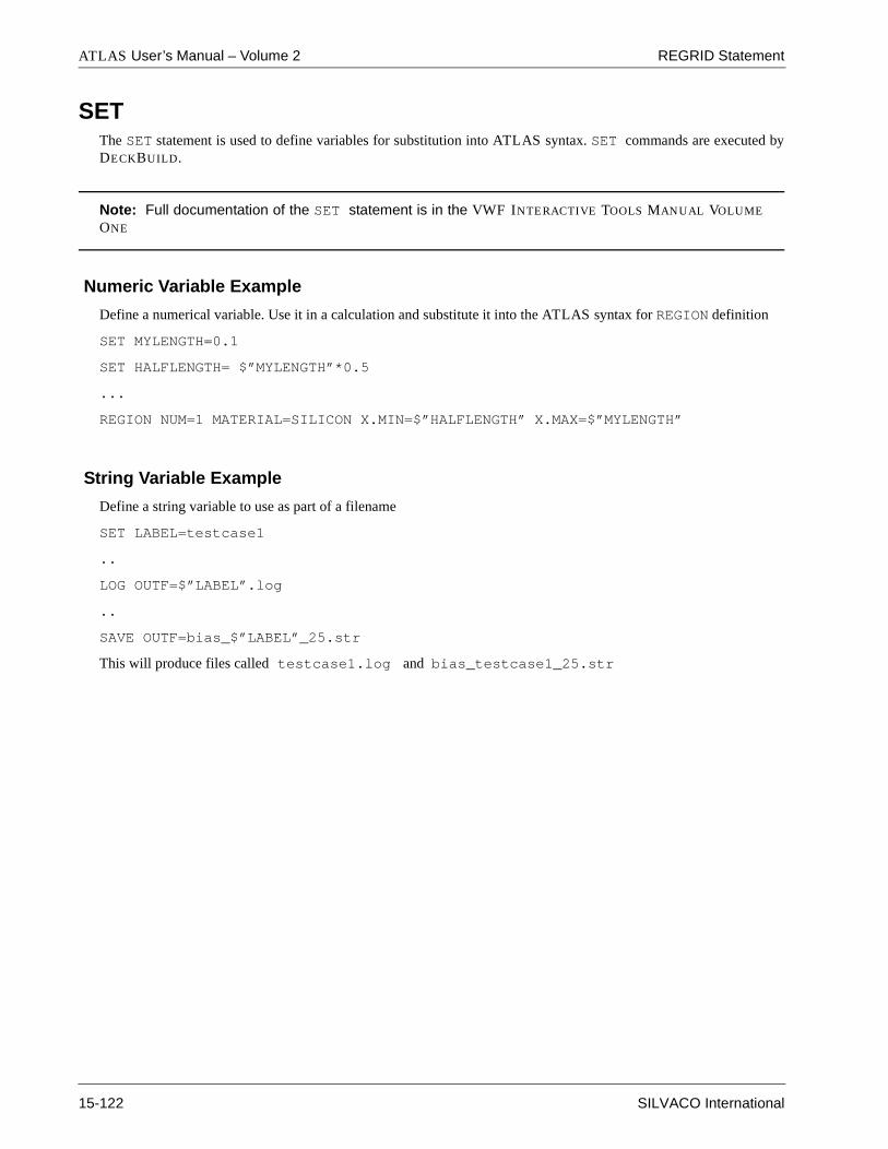
ATLAS User’s Manual – Volume 2 REGRID Statement
SETThe SET statement is used to define variables for substitution into ATLAS syntax. SET commands are executed byDECKBUILD.
Note: Full documentation of the SET statement is in the VWF INTERACTIVE TOOLS MANUAL VOLUMEONE
Numeric Variable Example
Define a numerical variable. Use it in a calculation and substitute it into the ATLAS syntax for REGION definition
SET MYLENGTH=0.1
SET HALFLENGTH= $”MYLENGTH”*0.5
...
REGION NUM=1 MATERIAL=SILICON X.MIN=$”HALFLENGTH” X.MAX=$”MYLENGTH”
String Variable Example
Define a string variable to use as part of a filename
SET LABEL=testcase1
..
LOG OUTF=$”LABEL”.log
..
SAVE OUTF=bias_$”LABEL”_25.str
This will produce files called testcase1.log and bias_testcase1_25.str
15-122 SILVACO International
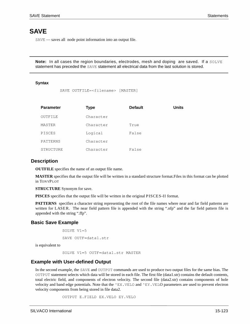
SAVE Statement Statements
lotted
erns arele is
. Thentents,
of holeon
SAVESAVE — saves all node point information into an output file.
Note: In all cases the region boundaries, electrodes, mesh and doping are saved. If a SOLVEstatement has preceded the SAVE statement all electrical data from the last solution is stored.
Syntax
SAVE OUTFILE=<filename> [MASTER]
Description
OUTFILE specifies the name of an output file name.
MASTER specifies that the output file will be written in a standard structure format.Files in this format can be pin TONYPLOT
STRUCTURE Synonym for save.
PISCES specifies that the output file will be written in the original PISCES-II format.
PATTERNS specifies a character string representing the root of the file names where near and far field pattwritten for LASER. The near field pattern file is appended with the string “.nfp” and the far field pattern fiappended with the string “.ffp”.
Basic Save Example
SOLVE V1=5
SAVE OUTF=data1.str
is equivalent to
SOLVE V1=5 OUTF=data1.str MASTER
Example with User-defined Output
In the second example, the SAVE and OUTPUT commands are used to produce two output files for the same biasOUTPUT statement selects which data will be stored in each file. The first file (data1.str) contains the default cototal electric field, and components of electron velocity. The second file (data2.str) contains components velocity and band edge potentials. Note that the ^EX.VELO and EY.VELO parameters are used to prevent electrvelocity components from being stored in file data2.
OUTPUT E.FIELD EX.VELO EY.VELO
Parameter Type Default Units
OUTFILE Character
MASTER Character True
PISCES Logical False
PATTERNS Character
STRUCTURE Character False
SILVACO International 15-123

ATLAS User’s Manual – Volume 2 SAVE Statement
SAVE OUTF=data1.str
OUTPUT HX.VELO HY.VELO CON.BAND VAL.BAND ^EX.VELO ^EY.VELO
SAVE OUTF=data2.str
Note: Contents of the saved file can be customised using the OUTPUT statement.
15-124 SILVACO International

SINGLEEVENTUPSET Statement Statements
.
SINGLEEVENTUPSETSINGLEEVENTUPSET — specifies the values of parameters used in Single Event Upset modeling in DEVICE3D orBLAZE3D.
Syntax
SINGLEEVENTUPSET <parameters>
Description
A1, A2, A3 and A4 are the first set of parameters for the length dependence of the charge generation pulse.
B1, B2, B3 and B4 are the second set of parameters for the length dependence of the charge generation pulse
Parameter Type Default Units
A1 Real
A2 Real
A3 Real
A4 Real
B1 Real
B2 Real
B3 Real
B4 Real
B.DENSITY Real 0 cm-3
BEAM.RADIUS Real 0 µm
DENSITY Real cm-3
ENTRYPOINT Real vector µm
EXITPOINT Real vector µm
PCUNITS Logical False
RADIALGAUSS Logical False
RADIUS Real µm
RESCALE Logical False
TFINAL.SEU Real
T0 Real c
TC Real c
TF Real sec
UNIFORM Logical False
SILVACO International 15-125

ATLAS User’s Manual – Volume 2 SINGLEEVENTUPSET Statement
B.DENSITY specifies the number of electron-hole pairs per unit volume or generated charge in pico Coulumbs permicron if the PCUNITS parameter is specified.
BEAM.RADIUS is the radius of the beam where the generation rate is maintained constant. Beyond this point thegeneration will decay by either an exponential or by a Gaussian function.
DENSITY specifies the number of electron-hole pairs per unit volume generated along the alpha particle track.
ENTRYPOINT specifies the x, y, and z coordinates of the beginning of the alpha particle track. The specified pointshould belong to the semiconductor region.
EXITPOINT specifies the x, y, and z coordinates of the end of the alpha particle track. The specified point shouldbelong to the semiconductor region.
PCUNITS sets the units of B.DENSITY to be pC per micron.
RADIALGAUSS specifies the Gaussian radial dependence of the charge generation pulse. By default the exponentialdependence is used.
RADIUS specifies the radius of the alpha particle track.
RESCALE causes nodal generation rates to be scaled by the ratio of the integral of the analytic generation ratedivided by the numerically intergrated value. NOTE: this may cause problems when the track radius approachesdevice dimensions.
TFINAL.SEU specifies the finish time for the track, this defaults to the finish time of the transient simulation ifTFINAL.SEU is not specified.
T0 specifies the peak in time of the charge generation pulse.
TC specifies the width of the charge generation pulse.
UNIFORM specifies that a uniform generation rate corresponding to that specified by the DENSITY parameter isapplied.
SEU Example
This statement specifies a track path, radius and density:
SINGLEEVENTUPSET ENTRYPOINT="1.5,2.0,0.0"\
EXITPOINT="1.0,1.0,4.0 RADIUS=0.05" \
DENSITY=1E18
Note: For user-defined Single Event Generation profiles the C-INTERPRETER function F3.RADIATE onthe BEAM statement can be used.
15-126 SILVACO International

SOLVE Statement Statements
SOLVESOLVE — instructs ATLAS to perform a solution for one or more specified bias points.
Syntax
SOLVE [<ion>] <dc> [<fp>][<ep>][<tp>][<ac>][<photo>] [<thermal>]
Parameter Type Default Units
AC.ANALYSIS Logical False
ANAME Character
AR.INDEX Real 1.0
AR.THICKNESS Real 0.0 microns
ASCII Logical False
AUTO Logical True
B<n> Real 0.0 W/cm2
CNAME Character
COMPLIANCE Real
CURVETRACE Logical False
CYCLES Integer 1
CYCLIC.BIAS Logical False
CYCLIC.RELAX Real 0.2
CYCLIC.TOL Real 1.0x10⁻⁵
DECAY Real s
DELTAV Real 0.1 V
DIRECT Logical False
DT Real 0 s
E.COMPL Real
E.CRIT Real 1.0x10⁻⁸
ELECTRODE Integer
ENDRAMP Real s
FREQUENCY Real Hz
FSTEP Real 0 Hz
GRAD Logical False
I<n> Real A/µm
SILVACO International 15-127

ATLAS User’s Manual – Volume 2 SOLVE Statement
IFINAL Real A/µm
IMULT Logical False
INAME Character
INDEX.CHECK Logical False
INITIAL Logical False
ION.CRIT Real 1.0
ION.ELEC Integer see Description
IONIZINT Logical False
IONLINES Integer 50 none
IONSTOP Logical True
ISTEP Real 0.0 A/µm
LAMBDA1 Real µm
LIT.STEP Real W/cm2
LOCAL Logical False
LRATIO Real 1.0
L.WAVE Real µm
MASTER Logical False
MAX.INNER Integer 25
MLOCAL Logical True
MULT.FREQ Logical False
N.BIAS Real V
NAME Character
NB1 Real V
NB2 Real V
NB3 Real V
NB4 Real V
NB5 Real V
NB6 Real V
NB7 Real V<B>
NB8 Real V
NFSTEPS Integer 0
Parameter Type Default Units
15-128 SILVACO International

SOLVE Statement Statements
NLAYERS Real 15
NSTEPS Integer 0
ONEFILEONLY Logical See Description
OUTFILE Character
P.BIAS Real
PB1 Real V
PB2 Real V
PB3 Real V
PB4 Real V
PB5 Real V
PB6 Real V
PB7 Real V
PB8 Real V
POWER<n> Real W
POWERFINAL Real W
PREVIOUS Logical False
PROJECT Logical False
PULSE.WIDTH Real s
Q<n> Real C/µm
QFACTOR Real 1.0 or previous value
QFINAL Real C/µm
QSTEP Real C/µm
RAMPTIME Real s
RAMP.LIT Logical False
SCAN.SPOT Real
S.OMEGA Real 1.0
SINUAMP.COMP Real 0.0
SINUVAR.COMP Real 0.0
SOR Logical False
SQPULSE Logical False
SS.LIGHT Real 0.001 W/cm2
Parameter Type Default Units
SILVACO International 15-129

ATLAS User’s Manual – Volume 2 SOLVE Statement
Description
Each SOLVE statement must specify an initial bias condition. Once any DC condition has been solved, either atransient or AC analysis may be performed. You may also solve for carrier generation due to incident light under DC,or AC analysis transient conditions.
dc is one or more of the DC bias parameters
fp is one or more of the file parameters
ep is one or more of the initial guess or estimate parameters. Estimate parameters are used to specify how the initialapproximation for the solution is to be obtained.
tp is one or more of the transient parameters. These parameters are used to specify data for transient analysis.
ac is one or more of the AC parameters. AC parameters are used to specify data for AC analysis.
ion is a set of the ionization integral parameters.
photo is one or more of the photogeneration parameters. Photogeneration parameters are used to specify illuminationdata.
therm is one or more of the thermal parameters. Thermal parameters are used for obtaining solutions inTHERMAL3D.
SS.PHOT Logical False
T <n> Real K
T.COMP Real 0 K
T.SAVE Real 0.0 s
TDELAY Real 0.0 s
TFALL Real 0.0 s
TRISE Real 0.0 s
TSAVE.MULT Real 1.0
TERMFINAL Real K
TERMINAL Integer all contacts
TOLERANCE Real 1.0x10⁻⁵
TRANS.ANALY Logical False
TSTOP Real
TWOFILESONLY Logical False
V<n> Real V
VFINAL Real V
VSTEP Real 0.0 V
VSS Real 0.1 V
Parameter Type Default Units
15-130 SILVACO International

SOLVE Statement Statements
DC Parameters
CURVETRACE initiates curve tracing. See also the CURVETRACE statement.
ELECTRODE specifies electrodes that you wish to add voltage and current increments (VSTEP and ISTEP) to. If nelectrodes are to be stepped, ELECTRODE should be an n-digit integer, where each of the digits is a separate electrodenumber. See also NAME.
I<name> specifies the applied current for a named electrode. One of several commonly used terminal names shouldbe specified. These names are as follows: gate, gg, drain, dd, source, bulk, substrate, emitter, ee, collector, cc,base, bb, anode, cathode, fgate, cgate, ngate, pgate, well, nwell, pwell, channel, and ground.No other user definednames are allowed.This parameter is used when current boundary conditions are selected (see the CONTACTstatement)
I<n> specifies the terminal current for electrode n. This parameter is used when current boundary conditions areselected (see the CONTACT statement). Normally, I defaults to the current from the previous bias point.It is more usualto use electrode names rather than numbers. This parameter is superceded by I<name>
IFINAL specifies the final current value for a set of bias increments. If IFINAL is specified, either ISTEP orNSTEPS must be specified.
IMULT specifies that the current (for current boundary conditions) be multiplied by ISTEP rather than incremented.
ISTEP specifies a current increment to be added to one or more electrodes, as specified by the electrode name appliedto the NAME parameter. If ISTEP is specified, either IFINAL or NSTEPS must also be specified.
N.BIAS specifies fixed electron quasi-Fermi potentials if electron continuity is not being solved. If N.BIAS is notspecified, then local quasi-Fermi potentials based on bias and doping are used. However, if FIX.QF is set in theMETHOD statement, quasi-Fermi levels will be set to the maximum bias.
NB<n> allows region by region specification of N.BIAS . The n index corresponds to the region index for which thespecified value of electron quasi-fermi level applies.
NAME specifies that the named electrode is to be ramped. Custom electrode names are supported by name. See alsothe V<name> parameter.
NSTEPS specifies the number of DC bias increments.
P.BIAS specifies fixed hole quasi-Fermi potentials if hole continuity is not being solved. If P.BIAS is not specified,then local quasi-Fermi potentials based on bias and doping are used. However, if FIX.QF is set in the METHODstatement, quasi-Fermi levels will be set to the minimum bias.
PB<n> allows region by region specification of P.BIAS. The n index corresponds to the region index for which thespecified value of hole quasi-fermi level applies.
Q<name> specifies the charge on a named electrode. These names are as follows: gate, gg, fgate, cgate, ngate,pgate.No other user defined names are allowed.This parameter is used when floating or charge boundary conditionsare selected (see the CONTACT statement)
Q<n> specifies the charge on electrode number n.It is more usual to use electrode names rather than numbers. Thisparameter is superceded by Q<name>
QFINAL specifies the final charge for a set of bias increments. If QFINAL is specified, either QSTEP or NSTEPSmust also be specified.
QSTEP specifies a charge increment to be added to one or more electrodes, as specified by the electrode nameapplied to the NAME parameter. If QSTEP is specified, either QFINAL or NSTEPS must also be specified.
V<name> specifies the bias voltage for a named electrode. One of several commonly used terminal names should bespecified. These names are as follows: gate, gg, drain, dd, source, bulk, substrate, emitter, ee, collector, cc, base,bb, anode, cathode, fgate, cgate, ngate, pgate, well, nwell, pwell, channel, and ground.No other user definednames are allowed.
V<n> specifies the bias voltage for electrode n. Normally, Vn defaults to the potential from the previous bias point. Itis more usual to use electrode names rather than numbers. This parameter is superceded by V<name>
SILVACO International 15-131

ATLAS User’s Manual – Volume 2 SOLVE Statement
Initial
ures in
. Thiselectrodes
minated
ram
VFINAL specifies the final voltage for a set of bias increments. If VFINAL is specified, either VSTEP or NSTEPSmust also be specified.
VSTEP specifies a voltage increment to be added to one or more electrodes, as specified by the electrode nameapplied to the NAME parameter. If VSTEP is specified, either VFINAL or NSTEPS must also be specified.
File Output Parameters
MASTER specifies that the output file selected by the OUTFILE parameter will be written in a standard structure filerather than in the older PISCES-II binary format.
ONEFILEONLY specifies that only one filename will be used to save solutions during a bias ramp. If this parameteris specified filename incrementation described under OUTFILE is not applied.This parameter is true by default unlessthe NAME or ELECTRODE parameters or transient simulationis specified. When CURVETRACE is used it is necessaryto explicitly set this parameter to false using ^ONEFILEONLY to save a different filename at each bias point.
OUTFILE specifies the name of the output file in which bias point solution information will be stored. If an electrodeis stepped so that more than one solution is generated by the SOLVE statement, the ASCII code of the last non-blankcharacter of the supplied file name will be incremented by one for each bias point in succession, resulting in a uniquefile per bias point.
Note: The output file specified by OUTFILE has a limit of 132 characters on a UNIX system, and eightcharacters on a PC system.
Initial Guess Parameters
INITIAL sets all voltages to zero. If this parameter is not specified for the first bias point in a given structure aSOLVE INIT statement is automatically inserted. The SOLVE INIT statement is always solved in zero carrier modewith no external elements attached.It is used to provide a good initial guess to subsequent solutions.
LOCAL specifies that the initial approximation should use local values of quasi-Fermi levels. Refer to the “Guesses” section of the Numerical Techniques Chapter for more detailed information.
MLOCAL specifies the modified local initial guess. This parameter is used when solved for carrier temperatthe energy balance models. If any energy balance model is specified, MLOCAL defaults to true.
PREVIOUS specifies that the previous solution as the initial approximation.
PROJ specifies that an extrapolation from the last two solutions will be used as an initial approximationparameter may be used if there are two or more existing solutions and equivalent bias steps are taken on any that are changed.
Note: If no initial guess parameters are specified, ATLAS will use PROJ wherever possible.
QFACTOR specifies as scaling factor to improve initial guesses when the QUANTUM model is used. Thisparameter should be ramped slowly from zero to unity at the start of quantum effect simulations.
Compliance Parameters
Compliance parameters define a current limit for a DC bias ramp or transient simulation. Simulation can be terby monitoring the current and checking against a user defined limit.
COMPLIANCE sets a limit on the current from the electrode which has been specified by the CNAME orE.COMPLIANCE parameter. When the COMPLIANCE value is reached, any bias ramp is stopped and the progcontinues withthe next line of the input file. The COMPLIANCE parameter is normally specified in A. If the GRADparameter is specified, COMPLIANCE is specified in A/V.
15-132 SILVACO International

SOLVE Statement Statements
E.COMPLIANCE specifies the electrode number to be used by the COMPLIANCE parameter. See also CNAME.
CNAME specifies the name of the electrode used by the COMPLIANCE.
GRAD specifies that the compliance value is a current/voltage gradient, and not a current value.
Transient Parameters
CYCLES specifies the number of periods to be simulated ( both FREQUENCY and TRANS.ANALY must be specifiedwhen this parameter is used ). ( synonym: PERIODS )
CYCLIC.BIAS specifies that a cyclic bias140 simulation is being performed. Cyclic biasing allows the effects ofrepeated trapazodial/square transient pulses (see SQPULSE) on the output characteristics to be determined, withouthaving to do the extremely large numbers of cycles. When CYCLIC.BIAS is specified, ATLAS will calculate a seriesof trapazodial/square pulses using the SQPULSE parameters. At the end of the third cycle (and at all subsequentcycles) the values of the potential (V), electron concentration (n), hole concentration (p) and trap probability ofoccupation (fT) will be modified according to the equation: x(k+1) = x(k) - CYCLIC.RELAX*((x(k) - x(k-1)) *dx(k))/(dx(k) - dx(k-1))
where x is a parameter such as V, n, p or fT at every node point, x(k) is the updated value calculated from the equation,k is the cycle number (with k+1 being the new update for parameter x), CYCLIC.RELAX is the relaxation factor,δx(k) is the difference between the simulated values of x at the start and beginning of the current cycle, while δx(k-1)is the equivalent for the previous cycle.
Steady state cyclic convergence is determined by comparing the normalizing sum of the updated values of V, n, p andfT with a tolerance value (CYCLIC.TOL).
CYCLIC.RELAX specifies the CYCLIC.BIAS relaxation factor (the recommended range for this parameter toensure stable convergence is between 0.2 and 1).
CYCLIC.TOL specifies the CYCLIC.BIAS tolerance factor.
DECAY specifies the time constant used for defining an exponential change in bias for transient simulation.
ENDRAMP applies any bias changes as linear ramps. ENDRAMP specifies the exact end of the ramp in running time;i.e. the ramp will start at t=t0 and end at t=ENDRAMP.
NSTEPS can be used to signal the end of the run; i.e., the final time would be t = t + NSTEPS* DT. This parametermay be used instead of the TSTOP parameter.
PULSE.WIDTH specifies the time constant used for sinusoidal nonlinear time domain simulation. If SQPULSE isspecified, PULSE.WIDTH is the width of the trapazodial/square pulse not including the rise and fall times.
RAMPTIME applies any bias changes as linear ramps. RAMPTIME specifies a ramp interval in seconds; i.e., theramp will begin at t=t0 and ends at t=t0 +RAMPTIME.
SINUAMP.COMP specifies that sinusoidal amplitude compliance will be used. The transient simulation will stop ifthe amplitude of a sinusoidal waveform is less than the value of SINUAMP.COMP.
SINUVAR.COMP specifies that sinusoidal variance compliance will be used. The transient simulation will stop if thechange in amplitude of a sinusoidal waveform is less than SINUVAR.COMP.
SQPULSE specifies that multiple trapazodial/square transient pulses will be applied. The pulse is controlled by theparameters: TDELAY, TRISE, PULSE.WIDTH, TFALL and FREQUENCY.
T.COMP specifies a temperature for temperature compliance. Once the specified temperature is obtained at somelocation on the mesh the solution process is discontinued.
T.SAVE specifies a time increment at which the device structure files are saved. Note: Actual time steps may notcorrespond to the user specified increment.
TDELAY specifies the time delay before the first cycle of multiple trapazodial/square transient pulses (SQPULSE)will be applied.
SILVACO International 15-133

ATLAS User’s Manual – Volume 2 SOLVE Statement
TFALL specifies the fall time for trapazodial/square transient pulses (SQPULSE).
TRISE specifies the rise time for trapazodial/square transient pulses (SQPULSE).
TRANS.ANALY specifies that transient analysis is being performed and that a sinusoid with a frequency, specified bythe FREQUENCY parameter, should be applied.
TSAVE.MULT specifies a multiplier the save time increment, T.SAVE, is multiplied by after each time a structure issaved.
TSTEP or DT specifies the time-step to be used. For automatic time-step runs, DT is used to select only the first timestep (see the METHOD statement).
TSTOP specifies the end of the time interval. If simulation begins at t=t0, it will end at t=TSTOP+t0.
AC Parameters
AC.ANALYSIS specifies that AC sinusoidal small-signal analysis should be performed after solving for the DCcondition. The full Newton method must be used for this analysis. This is typically specified with the statement
METHOD NEWTON CARRIERS=2
ANAME specifies the name of the electrode to which the AC bias will be applied. See also TERMINAL.If no ANAMEis specified, all electrodes have AC bias applied in turn.
AUTO selects an automatic AC analysis method. This method initially uses SOR. The DIRECT method will be used ifconvergence problems occur. We strongly recommend the use of the AUTO parameter.
DIRECT selects the direct AC solution method. This method is robust at all frequencies, but slow.
FREQUENCY specifies the AC analysis frequency. Analysis may be repeated at a number of different frequencies(without solving for the DC condition again) by specifying FSTEP. FREQUENCY can also be used to specify asinusoidal or square pulse frequency for transient simulations.
FSTEP specifies a frequency increment which is added to the previous frequency. If MULT.FREQ is specified, thefrequency will be multiplied by FSTEP.
MAX.INNER specifies the maximum number of SOR iterations.
MULT.FREQ specifies that the frequency will be multiplied by FSTEP, instead of added to FSTEP.
NFSTEPS specifies the number of times that the frequency is to be incremented by FSTEP.
S.OMEGA specifies the SOR parameter. This parameter is not the AC frequency.
SOR selects the SOR AC solution method. Although SOR is fast, it should only be used when you are performingsimulations at low frequencies. Low frequency can be defined here as at least an order of magnitude below the cutofffrequency.
TERMINAL specifies the electrode number to which the AC bias will be applied. Although more than one contactnumber may be specified (via concatenation), each will be solved separately. Each contact that is specified generates acolumn of the admittance matrix. If no TERMINAL is specified, all electrodes have AC bias applied in turn. See alsoANAME.
TOLERANCE specifies SOR convergence criterion.
VSS specifies the magnitude of the applied small-signal bias. The approach used for small-signal analysis constructs alinear problem based on derivatives calculated during Newton iterations, so adjusing VSS will generally not affect theresults.
Ionization Integral Parameters
Ionization parameters are used to calculate ionization integrals. No calculation will take place unless the IONIZINTparameter is specified.
15-134 SILVACO International

SOLVE Statement Statements
DELTAV since the electric field can be near zero at electrodes, the electric field line calculations begin at a distancefrom the electrode. A potential contour is drawn around the electrode at a distance where the potential is DELTAV lessthan the applied bias on the contact. Defaults to 0.1 V, but will typically need to be increased especially for powerdevices and heavily doped contact regions.
E.CRIT specifies the minimum electric field used to calculate integration integrals. Field lines will terminate whenthe field drops below E.CRIT.
INAME specifes the electrode name from which the electric field lines are calculated.The default is to use the sameas electrode as specified in NAME.
ION.CRIT specifies the critical value of the ionization integral used by IONSTOP to terminate the simulation. Whenthe critical value is reached, any bias ramp will be terminated and the next line of the input file will be executed.
ION.ELEC specifies the electrode from which the electric field lines are calculated. This parameter defaults to theelectrode which is being ramped (if any).
IONIZINT enables the calculation of ionization integrals along electric field lines.
IONLINES specifies the number of electric field lines to be calculated. Ionization integrals are calculated along eachline.
IONSTOP stops the bias ramp if integral is greater than 1.0
LRATIO specifies the ratio between the starting points of the electric field lines. An LRATIO value of between 0.5and 1.5 is recommended. LRATIO=1 means that the spacing between the starting points of the electric field lines isequal. LRATIO < 1 means more lines start towards the left hand side of the structure. LRATIO > 1 means more linesstart towards the right hand side.
Photogeneration Parameters
All these parameters require LUMINOUS to be licensed for correct operation.
AR.INDEX specifies the index of refraction for an antireflective coating.
AR.THICKNESS specifies the thickness in microns of an antireflective coating.
B<n> specifies the optical spot power associated with optical beam number n. The beam number must be an integerfrom 1 to 10. .
BEAM specifies the beam number of the optical beam when AC photogeneration analysis is performed. Unlike theELECTRODE parameter, this parameter can only be used to specify a single beam.
INDEX.CHECK specifies that the real and imaginary refractive indices used in the ray tracing of each beam will beprinted to the run-time output. This parameter can be used as confirmation of the input of user-defined refractiveindices or to check the default parameters.
L.WAVE specifies the luminous wavelength to use to calculate the luminous power estimate for radiativerecombination. If a positive value of L.WAVE is specified the luminous power will be saved in any log file specifiedfor that solution.
LAMBDA1 specifies the wavelength of the optical source (beam) number 1 for this solution. This parameter can beused to perform analysis of spectral response as a function of wavelength.
LIT.STEP selects the light intensity increment of all optical beams which have been specified. This parameter is usedwhen light intensity varies by stepping (similar to the VSTEP parameter). If LIT.STEP is specified, the NSTEPparameter should be used to select the number of steps.
RAMP.LIT specifies that the light intensity is to be ramped when transient simulations are performed. If RAMP.LITis specified, transient mode parameters such as RAMPTIME, TSTEP, and TSTOP must also be specified. TheRAMP.LIT parameter affects all specified optical beams (i.e., all beams are ramped).
SCAN.SPOT specifies a beam number for spot scanning. Spot scanning requires that the user specify the RAYSparameter of the BEAM statement. with this specification the incident light is split into the user specified number ofrays. During the spot scan solutions are obtained with the beam energy applied to each of the rays in sequence.
SILVACO International 15-135

ATLAS User’s Manual – Volume 2 SOLVE Statement
ges on
. The
sred.
SS.LIGHT specifies the intensity in the small signal part of the optical beam when small signal AC photogenerationanalysis is performed.
SS.PHOT specifies that small signal AC analysis will be performed on the optical beam selected by the BEAMparameter. When SS.PHOT is specified, other AC parameters (e.g., FREQUENCY, FSTEP, MAX.INNER,MULT.FREQ, NFSTEPS, S.OMEGA, and TOLERANCE) should also be specified. It is not necessary to specifythe AC.ANALYSIS parameter when performing small signal AC analysis on optical beams.
Thermal3D parameters
See also the section “Obtaining Solutions in THERMAL3D” of this manual.
POWER<n> specifies the power in watts on the n-th heat source.
POWERFINAL specifies the final power for a linearly ramped heat source.
T<n> specifies the temperature in K on the n-th heat sink.
TEMPFINAL specifies the final temperature for a linearly ramped heat sink.
DC Conditions Example
The following statement solves for a defined bias point and saves the solution to output file OutA. The voltaelectrodes other than the gate will keep the value from the previous SOLVE statement.
SOLVE VGATE=0.1 OUTFILE=OutA
Bias Stepping Example
In the next example, bias stepping is illustrated. The two SOLVE statements produce the following bias conditions:
The solutions for these bias points will be saved to the files OUT1, OUTA, OUTB, OUTC, OUTD and OUTEinitial approximation for each bias point is obtained directly from the preceding solution.
For bias points 4, 5, and 6, the program will use a PROJ to obtain an initial approximation. Since, starting with biapoint 4, both of its preceding solutions (bias points 2 and 3) only had the same electrode bias (number 1) alte
SOLVE Vdrain=.5 Vsub=–.5 OUTF=OUT1
SOLVE Vgate=1 VSTEP=1 VFINAL=5 NAME=gate OUTF=OUTA
Transient Simulation Example
The following sequence is an example of a time dependent solution. The METHOD statement specifies second-orderdiscretization, automatic time-step selection, and an automated Newton-Richardson procedure.
Bias Point Vgate Vdrain Vsub
1 0.0 0.5 -0.5
2 1.0 0.5 -0.5
3 2.0 0.5 -0.5
4 3.0 0.5 -0.5
5 4.0 0.5 -0.5
6 5.0 0.5 -0.5
15-136 SILVACO International

SOLVE Statement Statements
The first SOLVE statement then computes the solution for a device with 1V on the base electrode and 2V on thecollector in steady-state. The second SOLVE statement specifies that the base electrode is to be ramped to 2V over aperiod of 10 ns and is left on until 25 ns. Each solution is written to a file. The name of the file is incremented in amanner similar to that described for a DC simulation (UP1, UP2, etc.). Note that an initial time step had to be specifiedin this statement.
The third SOLVE statement ramps ther base down from 2V to - 0.5V in 20 ns (end of ramp is at =45 ns). The device isthen solved at this bias for another 55 ns (out to 100 ns). Each solution is again saved in a separate file (DOWN1,DOWN2, etc.).
No initial timestep was required since one had been estimated from the last transient solution from the previousSOLVE statement.
Finally, the fourth SOLVE statement performs the steady-state solution at Vbe = -0.5V and Vce = 2V.
METHOD 2ND TAUTO AUTONR
SOLVE Vbase=1 Vcollector=2
SOLVE Vbase=2 DT=1E-12 TSTOP=25E-9 RAMPTIME=10E-9 OUTF=UP1
SOLVE Vbase= –0.5 TSTOP=100E-9 RAMPTIME=20E-9 OUTF=DOWN1
SOLVE Vbase= –0.5 Vcollector=2
AC Analysis Example
The following example illustrates an application of the SOLVE statement for AC analysis. It is assumed that thedevice has three electrodes. This analysis is being performed after DC conditions are solved at V1 = 0V, 0.5V, 1.0V,1.5V, and 2.0V. A series of 10mV AC signals with frequencies of 1 MHz, 10 MHz, 100 MHz, 1 GHz, 10 GHz, and 100GHz are applied to each electrode in the device.
Ninety AC solutions will be performed (5 X 6 X 3 = 90).
SOLVE V1=0 V2=0 V3=0 VSTEP=0.5 NSTEPS=4 ELECT=1 \
AC FREQ=1E6 FSTEP=10 MULT.F NFSTEP=5 VSS=0.01
Photogeneration Examples
The following statement simulates two DC optical beams incident on the device with optical spot powers of 15 and 25
W/cm2.
SOLVE B1=15 B3=25
The next example shows how DC spot power of the two optical beams can be stepped simultaneously. Beam #1 will
increase to 35 W/cm2 and beam #3 will increase to 45 W/cm2.
SOLVE LIT.STEP=5.0 NSTEP=4
In the next example, the beams are ramped in the time domain. Beam #1 is ramped down to 0 W/cm2 and beam #3 is
ramped up to 100 W/cm2. The duration of the ramp is 1 ns. After the ramp, simulation will continue for 4 ns.
SOLVE B1=0 B3=100 RAMP.LIT TSTEP=2E-11 RAMPTIME=1E-9 TSTOP=5E-9
Next, the small signal response of a single beam is analyzed. First, ATLAS will solve the DC characteristics at thespecified optical spot powers. Then, the AC response of beam #1 will be calculated at a frequency of 10 MHz.
SOLVE B1=10 B3=20 BEAM=1 FREQUENCY=1e7 SS.PHOT SS.LIGHT=0.01
Finally, frequency stepping is used to look at the small signal AC frequency response of one of the beams. ACresponse is calculated at frequencies from 1kHz to 100MHz at each decade. The MULT.F parameter is used togeometrically increase the frequency.
SILVACO International 15-137
ATLAS User’s Manual – Volume 2 SOLVE Statement
SOLVE B1=10 B3=5 BEAM=1 SS.PHOT SS.LIGHT=0.01 \
MULT.F FREQUENCY=1E3 FSTEP=10 NFSTEP=6
Ionization Integral Example
Ionization integrals are used to estimate the breakdown voltage from analysis of the electric field. They can be used inzero carrier mode providing much faster simulation that conventional breakdown analysis. The ionization syntax usesthe parameter IONIZ to enable the ionization integral calculation. An equipotential contour is calculated at a potentialDELTAV from the contact NAME (or INAME). Electric field lines are started at distances along this potential contour.IONLINES sets the number of lines and LRATIO is the ratio of the distance between the starting points of the lines.The following syntax is for a PMOS transistor. See the on-line examples for other cases using ionization integrals.
IMPACT SELB
METHOD CARR=0
SOLVE VDRAIN=-1 VSTEP=-1 VFINAL=-20.0 NAME=DRAIN \
IONIZ IONLINES=50 LRATIO=0.9 DELTAV=1.2
Note: There are over 300 on-line examples supplied with ATLAS to provide examples of sequencesof SOLVE statements applied to practical problems for a variety of device technologies.
15-138 SILVACO International
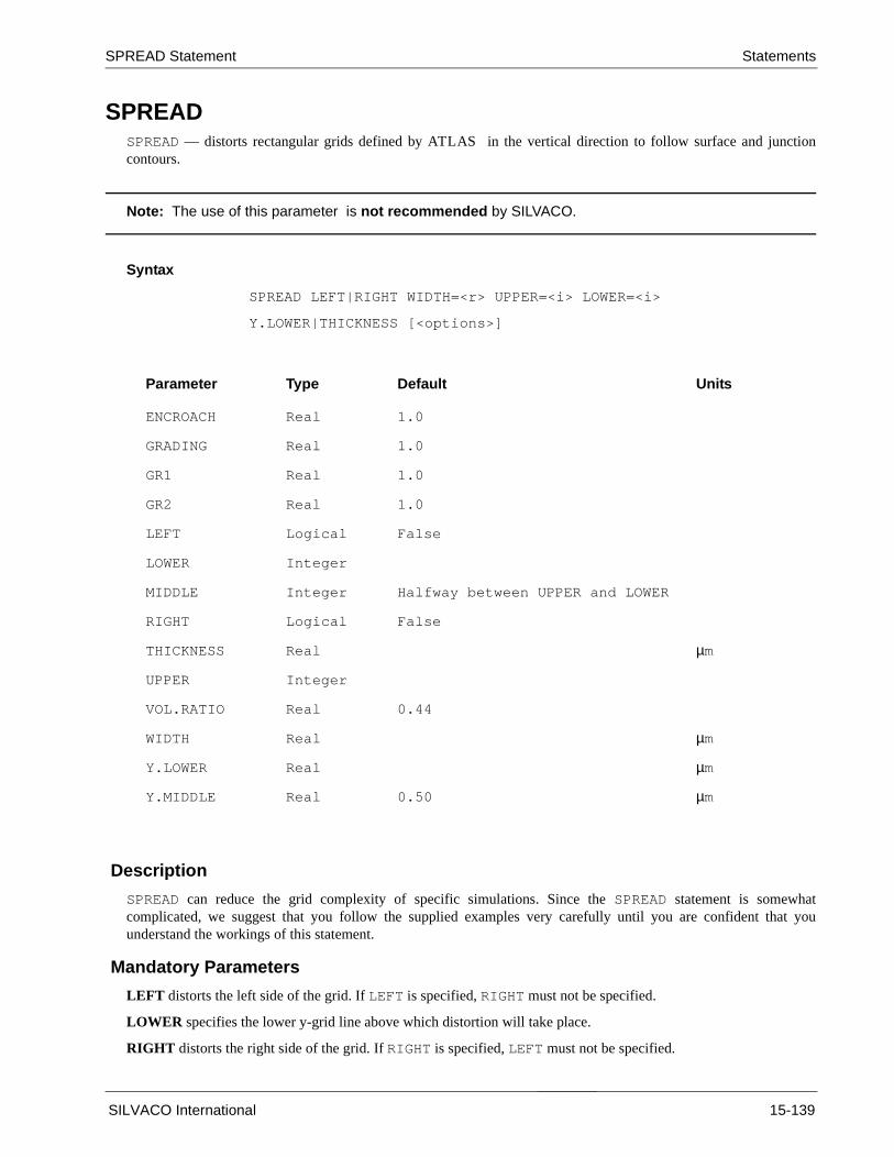
SPREAD Statement Statements
n
tat you
SPREADSPREAD — distorts rectangular grids defined by ATLAS in the vertical direction to follow surface and junctiocontours.
Note: The use of this parameter is not recommended by SILVACO.
Syntax
SPREAD LEFT|RIGHT WIDTH=<r> UPPER=<i> LOWER=<i>
Y.LOWER|THICKNESS [<options>]
Description
SPREAD can reduce the grid complexity of specific simulations. Since the SPREAD statement is somewhacomplicated, we suggest that you follow the supplied examples very carefully until you are confident thunderstand the workings of this statement.
Mandatory Parameters
LEFT distorts the left side of the grid. If LEFT is specified, RIGHT must not be specified.
LOWER specifies the lower y-grid line above which distortion will take place.
RIGHT distorts the right side of the grid. If RIGHT is specified, LEFT must not be specified.
Parameter Type Default Units
ENCROACH Real 1.0
GRADING Real 1.0
GR1 Real 1.0
GR2 Real 1.0
LEFT Logical False
LOWER Integer
MIDDLE Integer Halfway between UPPER and LOWER
RIGHT Logical False
THICKNESS Real µm
UPPER Integer
VOL.RATIO Real 0.44
WIDTH Real µm
Y.LOWER Real µm
Y.MIDDLE Real 0.50 µm
SILVACO International 15-139

ATLAS User’s Manual – Volume 2 SPREAD Statement
ickness
Å.factor.
THICKNESS specifies the thickness of the distorted region. Unless VOL.RATIO is set to 0 or 1, THICKNESS willusually move the positions of both the UPPER and LOWER grid lines. The Y.LOWER and THICKNESS parametersdefine the distorted grid region. Only one of these parameters should be specified.
UPPER specifies the upper y-grid line under which distortion will take place.
WIDTH specifies the width from the left or right edge (depending on whether LEFT or RIGHT is selected) of thedistorted area. The actual x coordinate specified by WIDTH (min[x]+ WIDTH for LEFT, max[x] + WIDTH for RIGHT)will lie in the middle of the transition region between distorted and undistorted grid regions.
Y.LOWER specifies the physical location in the distorted region to which the line specified by LOWER will be moved.The line specified by UPPER is not moved. The Y.LOWER and THICKNESS parameters define the distorted gridregion. Only one of these paramaters should be specified.
Optional Parameters
ENCROACH defines the abruptness of the transition between a distorted and nondistorted grid. The transition regionbecomes more abrupt with smaller ENCROACH factors (the minimum is 0.1).
Note: Depending on the characteristics of the undistorted grid, long. thin, or obtuse triangles may resultif too low an ENCROACH value is used.
GRADING specifies a grid ratio which produces a non-uniform grid in the distorted region. This parameter isidentical to the RATIO parameter in the X.MESH and Y.MESH statements.
GR1 and GR2 may be used instead of the GRADING parameter. GR1 and GR2 may be specified in conjunction withMIDDLE (y grid line) and Y.MIDDLE (location) so that GR1 specifies grading in the spread region from UPPER toMIDDLE, and GR2 specifies grading from MIDDLE to LOWER.
MIDDLE specifies the y-grid line that serves as a boundary between the grading specified by GR1 and the gradingspecified by GR2.
VOL.RATIO specifies the ratio of the downward displacement of the lower grid line to the net increase in thickness.The default (0.44) should be used for oxide-silicon interfaces. VOL.RATIO is ignored if Y.LOWER is specified.
Y.MIDDLE specifies the physical location in the distorted grid to which the line specified by MIDDLE will be moved.
Examples
This example spreads a uniform 400 Å of oxide to 1000 Å on the left side of the device. This increases oxide thby 600 Å. Because VOL.RATIO is not specified, the default (0.44) is used. Therefore, 0.44 X 600 = 264 Å of the netincrease will lie below the original 400 Å and 0.56 X 600 = 336 Å of the net increase will lie above the original 400The width of the spread region is 0.5 µm, and the oxide taper is quite gradual because of the high encroachment The grid is left uniform in the spread region.
# *** Mesh definition ***
MESH NX=30 NY=20 RECT
X.M N=1 L=0
X.M N=30 L=5
Y.M N=1 L=-.04
Y.M N=5 L=0
Y.M N=20 L=1 R=1.4
# *** Thin oxide ***
REGION IY.H=5 OXIDE NUM=1
15-140 SILVACO International
SPREAD Statement Statements
# *** Silicon substrate ***
REGION IY.L=5 SILICON NUM=2
# *** Spread ***
SPREAD LEFT W=0.7 UP=1 LO=4 THICK=0.1 MID=2 Y.MID=0.05
In the second example, the right side of the grid is distorted in order to follow a junction contour. The initial grid isassumed to be above. Y.LOWER is used so that there is no increase in the size of the device, just grid redistribution.When Y.LOWER is set to the junction, the ENCROACH parameter should be chosen such that the lower grid line(LOWER=10) follows the junction as closely as possible. The grid is graded so that grid lines are spaced closertogether as they approach the junction. Because the point specified by WIDTH lies in the middle of the transitionregion, it should be chosen to be slightly larger than the width of the doping “box.”
# *** Doping ***
DOPING UNIFORM N.TYPE CONC=1E15
DOPING GAUSS P.TYPE X.LEFT=1.5 X.RIGHT=2 \
PEAK= CONC=1.e19 RATIO=.75 JUNC=0.3
# *** Spread ***
SPREAD RIGHT W=0.7 UP=1 LO=4 THICK=0.3 MID=2 Y.MID=0.10
SILVACO International 15-141

ATLAS User’s Manual – Volume 2 SYMBOLIC Statements
SYMBOLIC
Note: In versions 3.0 and greater, the SYMBOLIC statement is no longer needed. All functions aremoved to the METHOD statement.
15-142 SILVACO International

SYSTEM Statement Statements
n a third
variable
SYSTEMSYSTEM — allows execution of any UNIX command within an input file
Note: The SYSTEM statement is executed by DECKBUILD and is fully documented in the VWFINTERACTIVE TOOLS MANUAL VOLUME ONE
Note: The SYSTEM command must be enabled using an option on the DECKBUILD Main_Control menuunder Category: Options.
ExamplesThe following command will remove all files test*.str before a SOLVE statement where the OUTF parameteris used
system \rm -rf test*.str
SOLVE .... OUTF=test0
The system command and the UNIX commands are case sensitive.
UNIX commands may be concatentated on a single line using the semicolon (;) operator. For example to ruparty program that reads and writes Silvaco format files with fixed names input.str and output.str.
SAVE OUTF=mysave.str
system mv mysave.str input.str; source myprog.exe; mv output.str myrestart.str
EXTRACT INIT INF=myrestart.str
The UNIX re-direct symbol > is not supported by the system command. The UNIX echo and sed syntax can beused instead to output values or variables to a given filename. For example to save the extracted value of$myvariable to the file myfile.
system echo $”myvariable” | sed -n “ w myfile”
15-143 SILVACO International

ATLAS User’s Manual – Volume 2 THERMOCONTACT Statement
d when
g order.
if
ame
THERMCONTACTTHERMCONTACT — specfies the position and properties of thermal contacts. This statement must be uselattice heating solutions are specified using GIGA or GIGA3D.
Syntax
THERMCONTACT NUMBER=<n> <position> [EXT.TEMPER=<n>] [ALPHA=<n>]
Description
At least one thermal contact statement must be specified when simulating lattice heating effects (MODELSLAT.TEMP). The THERMCONTACT statement must appear in the input deck before any METHOD statement.
position is a set of the position parameters described below. Either X.MIN, X.MAX, Y.MIN, and Y.MAXparameters are used to specify the exact postion of the contact or the ELEC.NUMBER parameter to specify anelectrode number that the thermal contact coincides with..
NUMBER specifies a thermal contact number from 1 to 20. Contact numbers should be specified in increasinThis parameters must be specified on all THERMCONTACT statements.
ALPHA specifies the reverse value of thermal resistance (α=1/RTH). This parameter may not be used ELEC.NUMBER parameter has been specified.
EXT.TEMPER specifies the external temperature.
Synonym: TEMPERATURE
Position Parameters
NAME specifies which region the THERMCONTACT statement applies to. Note that the name must match the nspecified in the NAME parameter of the REGION statement.
DEVICE specifies which device in MIXEDMODE simulation the THERMCONTACT statement applies to.
ELEC.NUMBER specifies an electrode number that the thermal contact is coincident with.
Parameter Type Default Units
ALPHA Real ∞ W/(cm2·K)
DEVICE Character
ELEC.NUMBER Integer
EXT.TEMPER Real 300 K
NAME Character
NUMBER Integer 1
X.MAX Real Right side of structure µm
X.MIN Real Left side of structure µm
Y.MAX Real Bottom of structure m µ
Y.MIN Real Top of structure µm
Z.MIN Real Front microns
Z.MAX Real Back microns
15-144 SILVACO International

THERMCONTACT Statement Statements
X.MIN specifies the left edge of the contact.
X.MAX specifies the right edge of the contact.
Y.MIN specifies the top edge of the contact.
Y.MAX specifies the bottom edge of the contact.
Z.MIN specifies the location of the front edge of the thermal contact.
Z.MAX specifies the location of the rear edge of the thermal contact.
Coordinate Definition Example
A thermal contact is located where y-coordinate values range from 10 µm to the bottom side of the structure and x-ccordinate values range from the left edge of the structure to the right edge of the structure (be default). The externaltemperature is set to 300K and a thermal resistance of 1 is added. Thus, the temperature at y = 10 µm will be greaterthan 300K once lattice heating effects occur.
THERMCONTACT NUM=1 Y.MIN=10 EXT.TEMP=300 ALPHA=1
Example Setting Thermal and Electrical Contacts Coincident
The next statement line creates a thermal contact at the location of electrode #4. An external temperature of 400K isspecified.
THERMCONTACT NUM=2 ELEC.NUM=4 EXT.TEMP=400
Note: Location and Parameters of thermal contacts are not stored in the ATLAS solution files.Therefore THERMCONTACT statements must be defined in each ATLAS run involving lattice heating.
SILVACO International 15-145

ATLAS User’s Manual – Volume 2 THERMOCONTACT Statement
TONYPLOTTONYPLOT — starts the graphical post-processor TONYPLOT
Note: The TONYPLOT statement is executed by DECKBUILD and is fully documented in the VWFINTERACTIVE TOOLS MANUAL VOLUME ONE
ExamplesAll graphics in ATLAS is performed by saving a file and loading the file into TONYPLOT. The command:
TONYPLOT
causes ATLAS to automatically save a structure file and plot it in TONYPLOT. The tonyplot window will appeardisplaying the material boundaries. Use the Plot:Display menu to see more graphics options.
This command will display the file myfile.str
tonyplot -st myfile.str
This command will overlay the results of myfile1.str and myfile2.str
tonyplot -overlay myfile1.str myfile2.str
Note: For documentation of the extensive features of TONYPLOT for graphical display and analysisconsult the TONYPLOT chapter of the VWF INTERACTIVE TOOLS MANUAL VOLUME ONE
15-146 SILVACO International

TITLE Statement Statements
TITLETITLE — specifies the title (up to 29 characters) that will appear in the standard output. If used the TITLE commandshould be the first statement inthe ATLAS input file.
Syntax
TITLE <string>
Example
This example causes the text “ *** CMOS p-channel device *** “ to be printed at the top of all ATLAS printouts,and screen displays.
TITLE *** CMOS p-channel device ***
Note: TITLE cannot be used with the automatic ATHENA to ATLAS interface feature of DECKBUILD
SILVACO International 15-147

ATLAS User’s Manual – Volume 2 TRAP Statement
ts their
e,
TRAPTRAP — activates bulk traps at discrete energy levels within the bandgap of the semiconductor and separameter values.
Syntax
TRAP DONOR|ACCEPTOR E.LEVEL=<r> DENSITY=<r> DEGEN=<v> <capture parameters>
Description
DEVICE specifies which device the statement applies to in MIXEDMODE simulation.
DONOR specifies a donor-type trap level.
ACCEPTOR specifies an acceptor-type trap level.
REGION specifies which region the traps apply to. If unspecified, the traps apply to all regions.
DENSITY sets the maximum density of states of the trap level.
DEGEN.FAC specifies the degeneracy factor of the trap level used to calculate the density.
E.LEVEL sets the energy of the discrete trap level. For acceptors E.LEVEL is relative to the conduction band edgfor donors it is relative to the valence band edge.
Parameter Type Default Units
ACCEPTOR Logical False
DEVICE Character
DEGEN.FAC Real undefined
DENSITY Real cm-3
DONOR Logical False
E.LEVEL Real eV
FAST Logical False
REGION Integer 0
SIGN Real cm2
SIGP Real cm2
TAUN Real s
TAUP Real s
15-148 SILVACO International

TRAP Statement Statements
Capture Parameters
Either the cross section or lifetime parameters should be used to define the capture parameters.
SIGN speccifies the capture cross section of the trap for electrons.
SIGP specifies the capture cross section of the trap for holes.
TAUN specifies the lifetime of electrons in the trap level.
TAUP specifies the lifetime of holes in the trap level.
Multiple Trap Level Definition Example
The following example sets three discrete trap levels within the silicon bandgap. These trap levels will capturecarriers, slowing the switching speed of any device. In this example the capture cross sections are used to define theproperties of each trap.
trap e.level=0.49 acceptor density=2.e15 degen=12 \
sign=2.84e-15 sigp=2.84e-14
trap e.level=0.41 acceptor density=1.e15 degen=12 \
sign=7.24e-16 sigp=7.24e-15
trap e.level=0.32 donor density=1.e15 degen=1 \
sign=1.00e-16 sigp=1.00e-17
Note: For distributed trap levels, see the DEFECT statement.
Note: For interface traps see the INTTRAP Statement .
Note: Spatial TRAP distributions in x, y or z directions must be defined on the DOPING statement
E.level for donor trap
E.level for acceptor trap
EC
Eta
EV
Etd
SILVACO International 15-149

ATLAS User’s Manual – Volume 2 UTMOST Statement
UTMOSTUTMOST — converts data from a ATLAS logfile format into an UTMOST logfile format.
Note: UTMOST 12.3.4 or later can read ATLAS format logfiles directly in batch mode. This statementis obsolete and its use is not recommended.
Syntax
UTMOST BIP|DIODE|MOS <input> OUTFILE=<fn> WIDTH=<n> [<elec>] <cntrl>
[TRANSLATE INFILE1=<filename>][<analysis>] [<parasites>]
Parameter Type Default Units
AC Logical False
ANODE Integer 1
APPEND Logical False
BASE Integer
BIP Logical False
BULK Integer
CATHODE Integer
COLLECTOR Integer
DEVICE Integer 1
DIODE Logical False
DRAIN Integer
EMITTER Integer
GATE Integer
INFILE Character
INTERNAL Logical False
LENGTH Real 1.0 µm
MESFET Logical False
MINSTEP Real 0.01 V
MOS Logical False
OUTFILE Character
POLARITY Integer 1 (n-type)
ROUTINE Integer 1
SOURCE Integer
15-150 SILVACO International

UTMOST Statement Statements
Description
You must specify a technology parameter (BIP, DIODE, or MOS), an input file (INFILE1=), and an output file(OUTFILE=). You may specify one or more of the optional electrode parameters
The INFILE parameter is used to convert up to nine ATLAS logfiles into a single UTMOST logfile. The ATLASlogfiles must be specified in the form:
INFILE1=<fn> INFILE2=<fn> INFILE3=<fn> . . .
where fn is the name of the logfile that you wish to convert.
OUTFILE specifies the name of a file in which I-V data will be stored in an UTMOST file format.
APPEND specifies that I-V data should be appended to the output file specified by OUTFILE2.
WIDTH is used to specify the width of the device. Electrode current is multiplied by the value of WIDTH before beingsaved in the logfile.
Technology Parameters
BIP creates an UTMOST bipolar transistor log file.
DIODE creates an UTMOST diode log file.
MOS creates an UTMOST MOSFET log file.
MESFET creates an UTMOST MESFET log file.
Electrode Parameters
Different electrode parameters may be specified with different technologies.
BIP Technology
BASE specifies the base electrode number.
COLLECTOR specifies the collector electrode numb.
EMITTER specifies the emitter electrode numb.
POLARITY indicates the device type. Polarity=1 specifies npn. Polarity=-1 specifies pnp.
MOS And MESFET Technologies
Note: If you have used the NAME parameter of the ELECTRODE statement to assign standard electrodenames (bulk, drain, gate, and source), it is not necessary to re-specify these names in the UTMOSTstatement.
BULK or SUBSTRATE specifies the bulk electrode number.
DRAIN specifies the drain electrode number.
TEMPERATURE Real 300 K
WELL Integer
WIDTH Real 1.0 µm
Parameter Type Default Units
SILVACO International 15-151
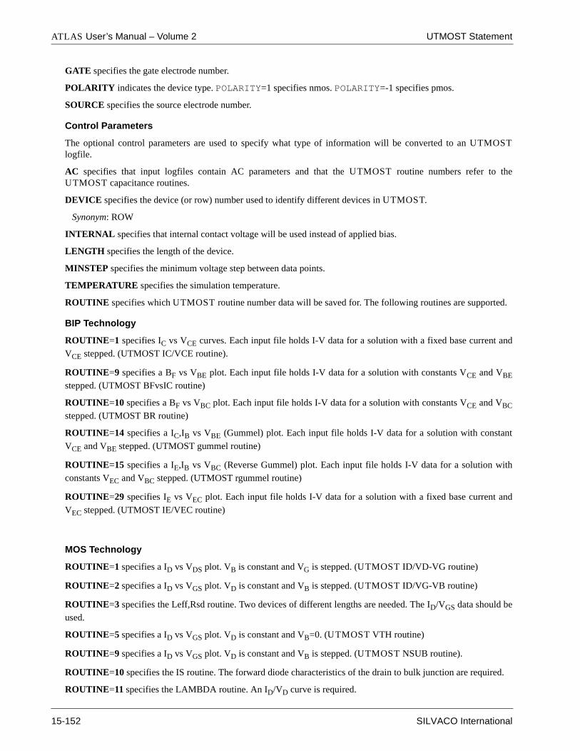
ATLAS User’s Manual – Volume 2 UTMOST Statement
GATE specifies the gate electrode number.
POLARITY indicates the device type. POLARITY=1 specifies nmos. POLARITY=-1 specifies pmos.
SOURCE specifies the source electrode number.
Control Parameters
The optional control parameters are used to specify what type of information will be converted to an UTMOSTlogfile.
AC specifies that input logfiles contain AC parameters and that the UTMOST routine numbers refer to theUTMOST capacitance routines.
DEVICE specifies the device (or row) number used to identify different devices in UTMOST.
Synonym: ROW
INTERNAL specifies that internal contact voltage will be used instead of applied bias.
LENGTH specifies the length of the device.
MINSTEP specifies the minimum voltage step between data points.
TEMPERATURE specifies the simulation temperature.
ROUTINE specifies which UTMOST routine number data will be saved for. The following routines are supported.
BIP Technology
ROUTINE=1 specifies IC vs VCE curves. Each input file holds I-V data for a solution with a fixed base current andVCE stepped. (UTMOST IC/VCE routine).
ROUTINE=9 specifies a BF vs VBE plot. Each input file holds I-V data for a solution with constants VCE and VBE
stepped. (UTMOST BFvsIC routine)
ROUTINE=10 specifies a BF vs VBC plot. Each input file holds I-V data for a solution with constants VCE and VBC
stepped. (UTMOST BR routine)
ROUTINE=14 specifies a IC,IB vs VBE (Gummel) plot. Each input file holds I-V data for a solution with constant
VCE and VBE stepped. (UTMOST gummel routine)
ROUTINE=15 specifies a IE,IB vs VBC (Reverse Gummel) plot. Each input file holds I-V data for a solution withconstants VEC and VBC stepped. (UTMOST rgummel routine)
ROUTINE=29 specifies IE vs VEC plot. Each input file holds I-V data for a solution with a fixed base current and
VEC stepped. (UTMOST IE/VEC routine)
MOS Technology
ROUTINE=1 specifies a ID vs VDS plot. VB is constant and VG is stepped. (UTMOST ID/VD-VG routine)
ROUTINE=2 specifies a ID vs VGS plot. VD is constant and VB is stepped. (UTMOST ID/VG-VB routine)
ROUTINE=3 specifies the Leff,Rsd routine. Two devices of different lengths are needed. The ID/VGS data should beused.
ROUTINE=5 specifies a ID vs VGS plot. VD is constant and VB=0. (UTMOST VTH routine)
ROUTINE=9 specifies a ID vs VGS plot. VD is constant and VB is stepped. (UTMOST NSUB routine).
ROUTINE=10 specifies the IS routine. The forward diode characteristics of the drain to bulk junction are required.
ROUTINE=11 specifies the LAMBDA routine. An ID/VD curve is required.
15-152 SILVACO International
UTMOST Statement Statements
ROUTINE=12 specifies the ETA routine. A set of ID/VGS data for different VDS is required.
ROUTINE=13 specifies the VMAX routine. A set of ID/VGS curves for small changes in VDS are required.
ROUTINE=14 specifies the U0 routine. A set of ID/VGS data is required.
ROUTINE=26 specifies a ID vs VGS plot. VB is constant and VD is stepped. (UTMOST ID/VG-VD routine).
MOS Capacitances
The following routines may be specified if both MOS and AC parameters are selected.
ROUTINE=1 specifies the CGSO routine. CGS vs. VGS data is required.
ROUTINE=2 specifies the CGDO routine. CGD vs. VGS data is required.
ROUTINE=5 specifies the CJ routine. CBD vs. VDS data is required.
ROUTINE=6 specifies the CJSW routine. CBD vs. VDS data is required.
ROUTINE=12 specifies the CJ/CJSW routine. CGD vs. VGS data is required for two different size drain areas.
Diode Technology
ROUTINE=1 specifies an I vs V plot. V is stepped. (UTMOST ID vs. VD routine)
Note: UTMOST 12.3.4 or later can read ATLAS format logfiles directly in batch mode. This statementis obsolete and its use is not recommended.
SILVACO International 15-153

ATLAS User’s Manual – Volume 2 X.MESH, Y.MESH, Z.MESH Statement
.
creasing
djacent
he
X.MESH, Y.MESH, Z.MESH<n>.MESH — specifies the location of grid lines along the <n>-axis in a rectangular mesh for 2-D or 3-D simulation
Note: The commands are equivalent in the x, y or z directions.
Syntax
X.MESH LOCATION=<l> (NODE=<n> [RATIO=<r>])| SPACING=<v>
Description
LOCATION specifies the location of the grid line.
NODE specifies mesh line index. There is a limit of 120 mesh lines. These mesh lines must be assigned in inorder.
RATIO specifies the ratio to use when interpolating grid lines between given locations. Spacing between agridlines will increase or decrease by the factor assigned to the RATIO parameter. A RATIO value of between 0.667and 1.5 is recommended. RATIO should not be used if SPACING is specified.
SPACING specifies the mesh spacing at the mesh locations specified by the LOCATION parameter. If the SPACINGparameter is specified, the NODE and RATIO parameters should not be specified. If the SPACING parameter is used tospecify mesh spacings, the NX, NY and NZ parameters of the MESH statement should not be specified. When tmesh spacings are specified using the SPACING parameter, the mesh size will be calculated.
Example Setting Fine Grid at A Junction
This example shows how to space grid lines closely around a junction at y=0.85 microns.
Y.MESH LOC=0.0 SPAC=0.2
Y.MESH LOC=0.85 SPAC=0.01
Y.MESH LOC=2 SPAC=0.35
Parameter Type Default Units
LOCATION Real µm
NODE Integer
RATIO Real 1
SPACING Real µm
15-154 SILVACO International

Appendix A:C-Interpreter Functions
Introduction
ATLAS has a built-in C language interpreter that allows many of the models contained in ATLAS to bemodified. In order to use the SILVACO C-INTERPRETER, C language functions containing analyticdescriptions of the model must be written. The C-INTERPRETER uses the ANSI standard definition of C.If you are not familiar with the C language, we suggest you refer to any of the popular C languagereferences such as the one written by Kernighan and Ritchie [74]. Additional information about the C-INTERPRETER can be found in the SILVACO C-INTERPRETER MANUAL.
The function arguments of the C-INTERPRETER functions and return values are fixed in ATLAS. Thuscare should be taken to ensure that the arguments and the return values for the functions match thoseexpected by ATLAS. To help the user, this release of ATLAS includes a set of templates for the availablefunctions. The C-INTERPRETER function template can be obtained by typing:
atlas -T filename
where filename is the name of a file where you want the template to be copied. The C-INTERPRETER
function template can also be obtained by accessing the template file through DECKBUILD.
This template file should be copied and edited when implementing user defined C-INTERPRETER
functions. In order to use the C-INTERPRETER function, the file name containing this function must bespecified in the appropriate ATLAS statement. The relevant statement names and parameters arelisted in the template file.
The following example shows how the C-INTERPRETER function “munsat” can be used to describe velocitysaturation for electrons.
First, examine the template file and find the template for “munsat”. The template should looksomething like this:
/*
* Electron velocity saturation model.
* Statement: MATERIAL
* Parameter: F.MUNSAT
*/
/* e electric field (V/cm) */
/* v saturation velocity (cm/s) */
/* mu0 low field mobility (cm^2/Vs) */
/* *mu return: field dependent mobility (cm^2/Vs) */
/* *dmde return: derivative of mu with e */
int munsat(double e, double v, double mu0, double *mu, double *dmde)
return(0); /* 0 - ok */
Here we see that the function is passed the electric field, the saturation velocity and the low fieldmobility. The function returns the field dependent mobility and the derivative of mobility with respectto electric field.
SILVACO International A-1

ATLAS User’s Manual - Volume 2
Note: It is important to properly calculate and return derivative values when specified, since theconvergence algorithms in ATLAS require these derivatives.
The return value is an error flag. In this case it is set to zero, indictating that the function wassuccesful (0=OK, 1=fail).
In this example the electron saturation velocity characteristic is changed to one which is akin to thatused for holes in silicon. This model could be specified by setting the B.ELE parameter to 1 but forexample purposes, the C-INTERPRETER function “munsat” is used instead. This will enable comparisonbetween the built-in model and the C-INTERPRETER model.
To implement the model, two lines additional lines of C code in the body of the function are specified asfollows:
/*
* Electron velocity saturation model.
* Statement: MATERIAL
* Parameter: F.MUNSAT
*/
/* e electric field (V/cm) */
/* v saturation velocity (cm/s) */
/* mu0 low field mobility (cm^2/Vs) */
/* *mu return: field dependent mobility (cm^2/Vs) */
/* *dmde return: derivative of mu with e */
int munsat(double e, double v, double mu0, double *mu, double *dmde)
*mu = mu0/(1.0+mu0*e/v);
*dmde = (*mu)*(*mu)/v;
return(0); /* 0 - ok */
The function then needs to be stored in a file. For example, the function may be stored in the file“test.lib”. The function is then introduced into a specific example by specifying the file name on theF.MUNSAT parameter in the MATERIAL statement as follows:
MATERIAL F.MUNSAT="test.lib"
When the input deck is executed the user’s C-INTERPRETER functions will be used in place of the built infunction. When trying this example, it is useful to place print statements (using the ‘printf ’ Ccommand) in the function to check that the function is working correctly.
A complete list of all the interpreter functions avialable in ATLAS is given in table 15-1 below.
Table 15-1. Complete list of available C-Interpreter functions in ATLAS
Statement Parameter Template Description
MATERIAL F.MUNSAT munsat () Electron velocity satura-tion model.
A-2 SILVACO International

C-Interpreter Functions
MATERIAL F.MUNSAT mupsat () Hole velocity saturation model.
MATERIAL F.BANDCOMP bandcomp () Temperature and composi-tion dependent band param-eters.
DOPING F.DOPING doping () Position dependent net doping.
DOPING F3.DOPING doping3() Position dependent net doping.
DOPING F.COMPOSIT composition () Position dependent compo-sition fractions.
MATERIAL F.EPSILON epsilon () Composition and tempera-ture dependent permittiv-ity.
MATERIAL F.FERRO ferro () Position and field depen-dent permittivity.
MATERIAL F.VSATN vsatn () Composition and tempera-ture dependent electron saturation velocity.
MATERIAL F.VSATP vsatp () Composition and tempera-ture dependent hole satu-ration velocity.
MATERIAL F.RECOMB recomb () Position, temperature, and concentration dependent recombination.
MATERIAL F.INDEX index () Wavelength dependent com-plex index of refraction.
BEAM F.REFLECT reflect () Reflection coefficient.
MATERIAL F.BGN bgn () Composition, temperature, and doping dependent band gap narrowing.
MATERIAL F.CONMUN conmun () Composition, temperature, and doping dependent elec-tron mobility.
MATERIAL F.CONMUP conmup () Composition, temperature, and doping dependent hole mobility.
BEAM F.RADIATE radiate () Generation rate as a func-tion of position.
BEAM F3.RADIATE radiate3 () Generation rate as a func-tion of position (3D).
MATERIAL F.TAUN taun () Electron SRH lifetime as a function of position.
Table 15-1. Complete list of available C-Interpreter functions in ATLAS
Statement Parameter Template Description
SILVACO International A-3

ATLAS User’s Manual - Volume 2
MATERIAL F.TAUP taup () Hole SRH lifetime as a function of position.
MATERIAL F.COPT copt () Radiative recombination rate as a function of com-position and temperature.
MATERIAL F.GAUN gaun () Electron Auguer rate as a function of composition and temperature.
MATERIAL F.GAUP gaup () Hole Auger rate as a func-tion of composition and temperature.
INTERFACE F.QF int_fixed_charge () Interface fixed charge as a function of position.
DEGREDAT F.NTA devdeg_nta () Interface acceptor trap density as a function of location.
DEGREDAT F.NTD devdeg_ntd () Interface donor trap den-sity as a function of location.
DEGREDAT F.SIGMAE devdeg_sigmae () Interface electron c apture cross-section.
DEGREDAT F.SIGMAH devdeg_sigmah () Interface hole capture cross-section.
INTTRAP F.DENSITY inte_acc_trap () Interface (acceptor/donor) trap density as a function of location.
DEFECT F.TFTDON tftdon () TFT donor trap densit yas a function of energy.
DEFECT F.TFTACC tftacc () TFT acceptor trap density as a function of energy.
IMPACT F.EDIIN ediin () Electron temperature coef-ficients for impact ion-ization.
IMPACT F.EDIIP ediip () Hole temperature coeffi-cients for impact ioniza-tion.
MATERIAL F.TAURN taurn () Energy dependent electron relaxation time.
MATERIAL F.TARUP taurp () Energy dependent hole relaxation time.
MODELS F.KSN fksn () Energy dependent electron Peltier coefficient.
Table 15-1. Complete list of available C-Interpreter functions in ATLAS
Statement Parameter Template Description
A-4 SILVACO International

C-Interpreter Functions
MODELS F.KSP fksp () Energy dependent hole Peltier coefficient.
BEAM F.OXGENERATE oxgenerate () Generation rate as a func-tion of position, time, and field (ORCHID).
DOPING F.OXCHARGE oxcharge () Position and current dependent net doping (ORCHID).
INTTRAP F.INTDONOR intdonor () Initial interface donor trap density, etc., as a function of position.
INTTRAP F.INTACCEPTO intacceptor () Initial interface acceptor trap density, etc., as a function of position.
INTTRAP F.INTPASSIVA intpassivated () Initial passivated trap density, tec., as a func-tion of position.
INTTRAP F.INTRATE intrate () Interfere passivation rate equation versus proton flux (ORCHID).
MODELS F.ALPHAA bulk_absorb () Bulk absorption coeffi-cient versus carrier den-sity and photon energy.
Table 15-1. Complete list of available C-Interpreter functions in ATLAS
Statement Parameter Template Description
SILVACO International A-5

ATLAS User’s Manual - Volume 2
[This page intentionally left blank]
A-6 SILVACO International

Appendix B:Material Systems
OverviewATLAS understands a library of materials for reference to material properties and models of variousregions in the semiconductor device. These materials are chosen to represent those most commonlyused by semiconductor physicists today. Users of BLAZE or BLAZE3D will have access to all of thesematerials. S-PISCES or DEVICE3D users will have only access to Silicon and Polysilicon.
S-PISCES is designed to maintain backward compatibility with the standalone program SPISCES2version 5.2. In the SPISCES2 syntax, certain materials could be used in the REGION statement just byusing their name as logical parameters. This syntax is still supported.
Semiconductors, Insulators and ConductorsAll materials in ATLAS are strictly defined into three classes as either semiconductor materials,insulator materials or conductors. Each class of material has particular properties to which all usersshould be aware.
Semiconductors
All equations specified by the user’s choice of models are solved in semiconductor regions. Allsemiconductor regions must have a band structure defined in terms of bandgap, density of states,affinity etc. The parameters used for any simulation can be echoed to the run-time output usingMODELS PRINT. For complex cases with mole fraction dependent models these quantities can be seenin Tonyplot by specifying OUTPUT BAND.PARAM and saving a solution file.
Any semiconductor region that is defined as an electrode is then considered to be a conductor region.This is typical for polysilicon gate electrodes.
Insulators
In insulator materials only the Poisson and lattice heat equations are solved. Therefore for isothermalsimulations, the only parameter required for an insulator is dielectric permittivity defined usingMATERIAL PERM=<n>.
Materials usually considered as insulators (eg. SiO2) can be treated as semiconductors using BLAZE,however all semiconductor parameters are then required.
Conductors
All conductor materials must be defined as electrodes. Conversely all electrode regions are defined asconductor material regions. If a file containing regions of a material known to be a conductor are readin, these regions will automatically become un-named electrodes. As noted bellow if the file containsmaterials that are unknown, these region will become insulators.
During electrical simulation only the electrode boundary nodes are used. Nodes that are entirelywithin an electrode region are not solved. Any quantities seen inside a conductor region in TONYPLOTare spurious. Only optical ray tracing and absorption for LUMINOUS and lattice heating are solvedinside of conductor/electrode regions.
SILVACO International B-1

ATLAS User’s Manual - Volume 2
Unknown Materials
If a mesh file is read containing materials not in Table B-1 these will automatically become insulatorregions with a relative permittivity of 3.9. All user-defined materials from ATHENA, irrespective ofthe material name chosen by the user, will also become such insulator materials.
B-2 SILVACO International

Material Systems
ATLAS Materials
ATLAS materials are listed in Table B-1 below.
Table B-1. The ATLAS Materials
Single Element Semiconductors
Silicon1 Poly2 Germanium Diamond
Binary Compound Semiconductors
GaAs 3 GaP CdSe SnTe
SiGe InP CdTe ScN
a-SiC InSb HgS GaN
b-SiC InAs HgSe AlN
AlP ZnS HgTe InN
AlAs ZnSe PbS BeTe
AlSb ZnTe PbSe
GaSb CdS PbTe
Ternary Compound Semiconductors
AlGaAs GaSbP InAlAs GaAsP
InGaAs GaSbAs InAsP HgCdTe
InGaP InGaN AlGaN
Quaternary Compound Semiconductors
InGaAsP AlGaAsP AlGaAsSb InAlGaN
InGaNAs InGaNP AlGaNAs AlGaNP
AlInNAs AlInNP InAlGaAs InAlGaP
InAlAsP
SILVACO International B-3

ATLAS User’s Manual - Volume 2
Notes
1. The material models and parameters of Silicon are identical to those of S-PISCES version 5.2. Users should beaware that although these band parameters may be physically inaccurate compared to bulk silicon measurements,most other material parameters and models are empirically tuned using these band parameters.
2. Polysilicon is treated differently depending on how it is used. In cases where it is defined as an electrode, it is treatedas a conductor. It can also be used as a semiconductor such as in a polysilicon emitter bipolars.
3. The composition of SiGe is the only binary compound that can be varied to simulate the effects of band gap varia-tions.
4. Conductor names are only associated with electrodes. They are used for the specification of thermal conductivitiesand complex index of refraction and for display in TonyPlot.
Rules for Specifying Compound Semiconductors
The rules for specifying the order of elements for compound semiconductors are derived from the rulesused by the International Union of Pure and Applied Chemistry:
1. Cations appear before anions.
2. When more than one cation is present the order progresses from the element with the largest atomic number to the element with the smallest atomic number.
3. The order of anions should be the in order of the following list: B, Si, C, Sb, As, P, N, H, Te, Se, S, At, I, Br, Cl, O, and F.
4. The composition fraction x is applied to the cation listed first.
5. The composition y is applied to the anion listed first.
To accomodate popular conventions, there are several exceptions to these rules.
Insulators
Vacuum Oxide Nitride Si3N4
Air SiO2 SiN Sapphire
Ambient
Conductors4
Polysilico2
Palladium TiW TaSi
Aluminum Cobalt Copper PaSi
Gold Molybdenum Tin PtSi
Silver Lead Nickel MoSi
AlSi Iron WSi ZrSi
Tungsten Tantalum TiSi AlSi
Titanium AlSiTi NiSi Conductor
Platinum AlSiCu CoSi Contact
B-4 SILVACO International

Material Systems
•SiGe: The composition fraction x applies to the Ge component. SiGe is then specified as Si(1-x)Ge(x),an exception to rule #4.
•AlGaAs : This is specified as Al(x)Ga(1-x)As. This is an exception to rule #2.
•InGaAsP: The convention In(1-x)Ga(x)As(y)P(1-y) as set forth by Adachi is used. This is an exception torule #4.
SILVACO International B-5

ATLAS User’s Manual - Volume 2
Silicon and PolysiliconThe material parameters defaults for Polysilicon are identical to those for Silicon. The followingparagraphs describe some of the material parameter defaults for Silicon and Polysilicon.
Note: Within the Physics section of this manual, a complete description is given of each model. Theparameter defaults listed in Chapter Three are all Silicon material defaults.
Silicon and Polysilicon Band Parameters
Silicon and Polysilicon Dielectric Properties
Silicon and Polysilicon Default Mobility Parameters
The default mobility parameters for Silicon and Poly are identical in all cases. The defaults useddepend on the particular mobility models in question. A full description of each mobility model andtheir coefficients are given in Chapter 3.
Table B-4 contains the silicon and polysilicon default values for the low field constant mobility model.
Table B-2. Band parameters for Silicon and Poly
MaterialEg300
eVα β Nc300
per ccNv300per cc
χeV
Silicon 1.08 4.73x10⁻⁴ 636.0 2.8x10¹⁹ 1.04x10¹⁹ 4.17
Poly 1.08 4.73x10⁻⁴ 636.0 2.8x10¹⁹ 1.04x10¹⁹ 4.17
Table B-3. Static dielectric constants for Silicon and Poly
Material Dielectric Constant
Silicon 11.8
Poly 11.8
Table B-4. Lattice Mobility Model Defaults for Silicon and Poly
Material MUNcm2/Vs
MUPcm2/Vs
TMUN TMUP
Silicon 1000.0 500.0 1.5 1.5
Poly 1000.0 500.0 1.5 1.5
B-6 SILVACO International
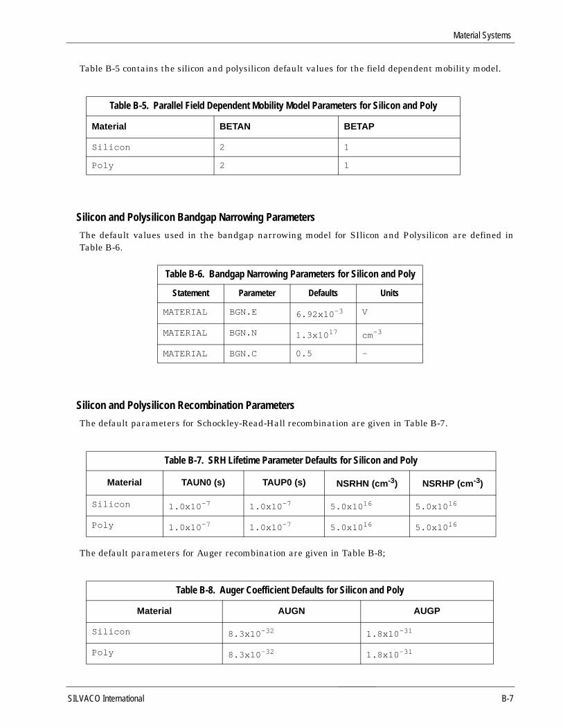
Material Systems
Table B-5 contains the silicon and polysilicon default values for the field dependent mobility model.
Silicon and Polysilicon Bandgap Narrowing Parameters
The default values used in the bandgap narrowing model for SIlicon and Polysilicon are defined inTable B-6.
Silicon and Polysilicon Recombination Parameters
The default parameters for Schockley-Read-Hall recombination are given in Table B-7.
The default parameters for Auger recombination are given in Table B-8;
Table B-5. Parallel Field Dependent Mobility Model Parameters for Silicon and Poly
Material BETAN BETAP
Silicon 2 1
Poly 2 1
Table B-6. Bandgap Narrowing Parameters for Silicon and Poly
Statement Parameter Defaults Units
MATERIAL BGN.E 6.92x10⁻³ V
MATERIAL BGN.N 1.3x1017 cm-3
MATERIAL BGN.C 0.5 —
Table B-7. SRH Lifetime Parameter Defaults for Silicon and Poly
Material TAUN0 (s) TAUP0 (s) NSRHN (cm-3) NSRHP (cm-3)
Silicon 1.0x10 -7 1.0x10 -7 5.0x10 16 5.0x10 16
Poly 1.0x10 -7 1.0x10 -7 5.0x10 16 5.0x10 16
Table B-8. Auger Coefficient Defaults for Silicon and Poly
Material AUGN AUGP
Silicon 8.3x10 -32 1.8x10 -31
Poly 8.3x10 -32 1.8x10 -31
SILVACO International B-7

ATLAS User’s Manual - Volume 2
Silicon and Polysilicon Impact Ionization Coefficients
The default values for the SELB impact ionization coefficients are given in Table B-9.
Silicon and Polysilicon Thermal Parameters
The default values used for thermal conductivity and capacity are given in Table B-10.
Silicon And Polysilicon Effective Richardson Coefficients
Table B-9. Impact Ionization Coefficients for Silicon and Poly
Parameter Value
EGRAN 4.0x10⁵
BETAN 1.0
BETAP 1.0
AN1 7.03x10⁵
AN2 7.03x10⁵
BN1 1.231x10⁶
BN2 1.231x10⁶
AP1 6.71x10⁵
AP2 1.582x10⁶
BP1 1.693x10⁶
BP2 2.036x10⁶
Table B-10. Effective Richardson Coefficients for Silicon and Poly
Material TCA TCB TCC HCA HCB HCC HCD
Silicon 0.03 1.56x10⁻³ 1.65x10⁻⁶ 1.97 3.6x10⁻⁴ 0.0 -3.7x10⁴
Poly 0.03 1.56x10⁻³ 1.65x10⁻⁶ 1.97 3.6x10⁻⁴ 0.0 -3.7x10⁴
B-8 SILVACO International

Material Systems
Table B-11. Effective Richardson Coefficients for Silicon and Poly
Material ARICHN (A/cm2/K2) ARICHP (A/cm2/K2)
Silicon 110.0 30.0
Poly 110.0 30.0
SILVACO International B-9

ATLAS User’s Manual - Volume 2
The Al(x)Ga(1-x)As Material System
AlGaAs Recombination Parameters.
The default recombination parameters for AlGaAs are given in Table B-12.
GaAs and AlGaAs Impact Ionization Coefficients.
The default values for the SELB impact ionization coefficients used for GaAs are given in Table B-13.AlGaAs uses the same values as GaAs.
Table B-12. Default Recombination Parameters for AIGaAs
Parameter Value Equation
TAUN0 1.0x10⁻⁹ 3-213
TAUP0 1.0x10⁻⁸ 3-213
COPT 1.5x10⁻¹⁰ 3-226
AUGN 5.0x10⁻³⁰ 3-227
AUGP 1.0x10⁻³¹ 3-227
Table B-13. Impact Ionization Coefficients for GaAs
Parameter Value
EGRAN 0.0
BETAN 1.82
BETAP 1.75
EGRAN 0.0
AN1 1.889x10⁵
AN2 1.889x10⁵
BN1 5.75x10⁵
BN2 5.75x10⁵
AP1 2.215x10⁵
AP2 2.215x10⁵
BP1 6.57x10⁵
BP2 6.57x10⁵
B-10 SILVACO International

Material Systems
AlGaAs Thermal Parameters.
The default thermal parameters used for AlGaAs are given in Table B-14.
GaAs Effective Richardson Coefficients.
The default values for the effective Richardson coefficients for GaAs are 6.2875 A/cm2/K2 for electronsand 105.2 A/cm2/K2 for holes.
Table B-14. Default Thermal Parameters for GaAs
Parameter Value
TCA 2.27
HCA 1.738
SILVACO International B-11

ATLAS User’s Manual - Volume 2
The In(1-x)Ga(x)As(y)P(1-y) System
InGaAsP Thermal Parameters.
The default material thermal models for InGaAsP assumes lattice-matching to InP. The materialdensity is then given by;
The specific heat for InGaAsP is given by;
The thermal resistivities of InGaAsP are linearly interpolated from Table B-15.
The default thermal properties of the binary compounds in the InGaAsP system are given in Table B-16.
Table B-15. Thermal Resistivities for InGaAsP Lattice-Matched to InP
Composition Fraction y Thermal Resistivity (deg(cm/w)
0.0 1.47
0.1 7.05
0.2 11.84
0.3 15.83
0.4 19.02
0.5 21.40
0.6 22.96
0.7 23.71
0.8 23.63
0.9 22.71
1.0 20.95
Table B-16. Default Thermal Properties of InP InAs GaP and GaAs
Material Thermal Capacity (J/cm3) Thermal Resistivity (deg(cm/W)
InP 1.543 1.47
InAs 1.994 3.70
GaP 1.292 1.30
GaAs 1.738 2.27
ρ 4.791 0.575y.composition 0.138y.composition+ +=
Cp 0.322 0.026y.composition 0.008y.composition–+=
B-12 SILVACO International

Material Systems
The default thermal properties for the terniary compounds in the InGaAsP system: In(1-x)Ga(x)As,In(1-x)Ga(x)P, InAs(y)P(1-y), and GaAs(y)P(1-y) are given, as a function of composition fraction, by linearinterpolations from these binary compounds.
SILVACO International B-13
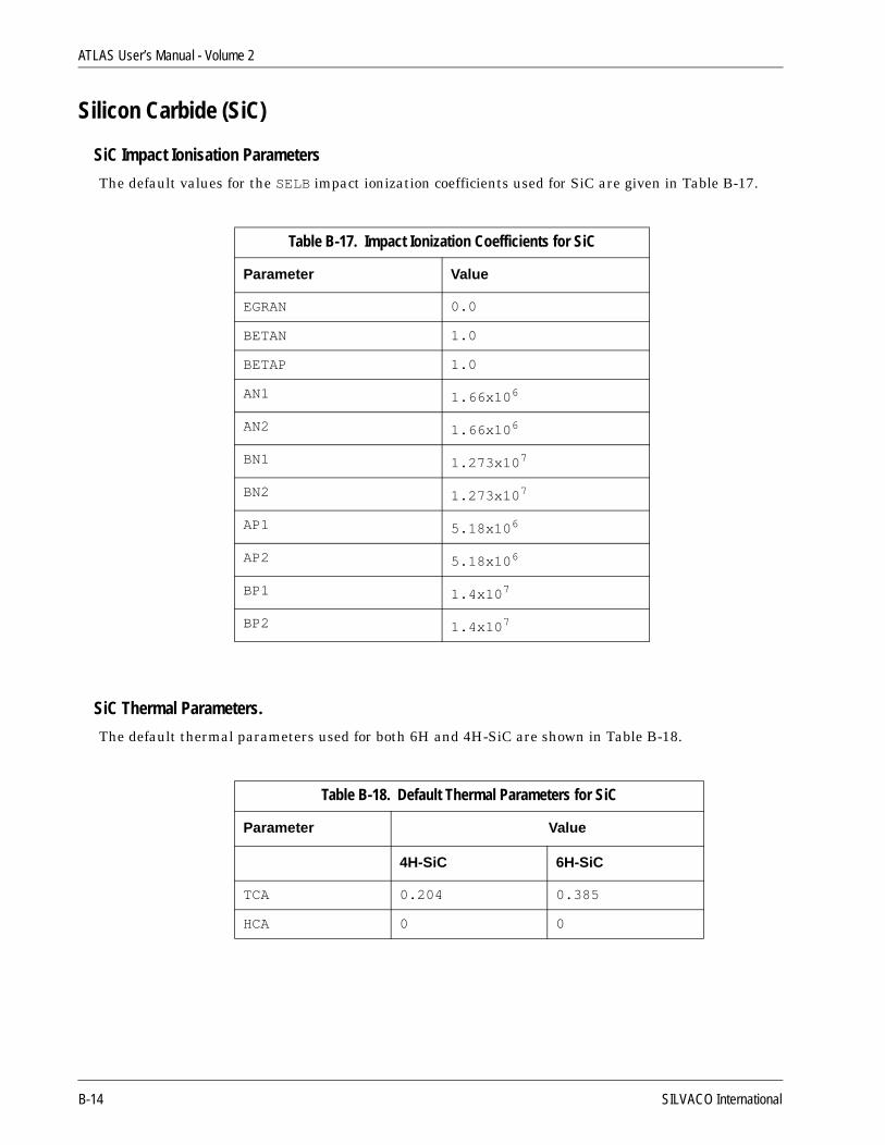
ATLAS User’s Manual - Volume 2
Silicon Carbide (SiC)
SiC Impact Ionisation Parameters
The default values for the SELB impact ionization coefficients used for SiC are given in Table B-17.
SiC Thermal Parameters.
The default thermal parameters used for both 6H and 4H-SiC are shown in Table B-18.
Table B-17. Impact Ionization Coefficients for SiC
Parameter Value
EGRAN 0.0
BETAN 1.0
BETAP 1.0
AN1 1.66x10⁶
AN2 1.66x10⁶
BN1 1.273x10⁷
BN2 1.273x10⁷
AP1 5.18x10⁶
AP2 5.18x10⁶
BP1 1.4x10⁷
BP2 1.4x10⁷
Table B-18. Default Thermal Parameters for SiC
Parameter Value
4H-SiC 6H-SiC
TCA 0.204 0.385
HCA 0 0
B-14 SILVACO International
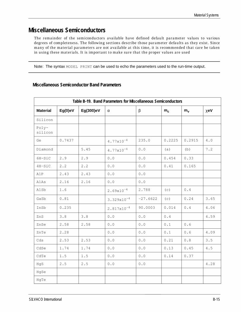
Material Systems
Miscellaneous SemiconductorsThe remainder of the semiconductors available have defined default parameter values to variousdegrees of completeness. The following sections describe those parameter defaults as they exist. Sincemany of the material parameters are not available at this time, it is recommended that care be takenin using these materials. It is important to make sure that the proper values are used
Note: The syntax MODEL PRINT can be used to echo the parameters used to the run-time output.
Miscellaneous Semiconductor Band Parameters
Table B-19. Band Parameters for Miscellaneous Semiconductors
Material Eg(0)eV Eg(300)eV α β mc mv χeV
Silicon
Poly-silicon
Ge 0.7437 4.77x10⁻⁴ 235.0 0.2225 0.2915 4.0
Diamond 5.45 4.77x10⁻⁴ 0.0 (a) (b) 7.2
6H-SiC 2.9 2.9 0.0 0.0 0.454 0.33
4H-SiC 2.2 2.2 0.0 0.0 0.41 0.165
A1P 2.43 2.43 0.0 0.0
A1As 2.16 2.16 0.0 0.0
A1Sb 1.6 2.69x10⁻⁴ 2.788 (c) 0.4
GaSb 0.81 3.329x10⁻⁴ -27.6622 (c) 0.24 3.65
InSb 0.235 2.817x10⁻⁴ 90.0003 0.014 0.4 4.06
ZnS 3.8 3.8 0.0 0.0 0.4 4.59
ZnSe 2.58 2.58 0.0 0.0 0.1 0.6
ZnTe 2.28 0.0 0.0 0.1 0.6 4.09
Cds 2.53 2.53 0.0 0.0 0.21 0.8 3.5
CdSe 1.74 1.74 0.0 0.0 0.13 0.45 4.5
CdTe 1.5 1.5 0.0 0.0 0.14 0.37
HgS 2.5 2.5 0.0 0.0 4.28
HgSe
HgTe
SILVACO International B-15

ATLAS User’s Manual - Volume 2
Notes
(a). Nc300 = 5.0x10¹⁸
(b). Nv300 = 1.8x10¹⁹
(c). mc(X) = 0.39
mc(G) = 0.09
Nc = Nc(X) + Nc(G)
(d). mc(G) = 0.047
mc(L) = 0.36
Nc = Nc(G) + Nc(L)
Miscellaneous Semiconductor Dielectric Properties
PbS 0.37 0.37 0.0 0.0 0.25 0.25
PbSe 0.26 0.26 0.0 0.0 0.33 0.34
PbTe 0.29 0.29 0.0 0.0 0.17 0.20 4.6
SnTe 0.18 0.18 0.0 0.0
ScN 2.15 2.15 0.0 0.0
GaN 3.45 3.45 0.0 0.0 0.172 0.259
A1N 6.28 6.28 0.0 0.0 0.314 0.417
InN 1.89 1.89 0.0 0.0 0.11 0.17
BeTe 2.57 2.57 0.0 0.0
Table B-20. Static Dielectric Constants for Miscellaneous Semiconductors
Material Dielectric Constant
Ge 16.0
Diamond 5.5
6H-SiC(a) 9.66
4H-SiC(b) 9.72
AlP 9.8
AlAs 12.0
AlSb 11.0
Table B-19. Band Parameters for Miscellaneous Semiconductors
Material Eg(0)eV Eg(300)eV α β mc mv χeV
B-16 SILVACO International

Material Systems
Miscellaneous Semiconductor Mobility Properties
GaSb 15.7
InSb 18.0
ZnS 8.3
ZnSe 8.1
CdS 8.9
CdSe 10.6
CdTe 10.9
HgS
HgSe 25.0
HgTe 20.
PbS 170.0
PbSe 250.0
PbTe 412.0
SnTe
ScN
GaN 9.5
AlN 9.14
InN 19.6
BeTe
Table B-21. Mobility Parameters for Miscellaneous Semiconductors
Material MUNO (cm2/Vs) MUPO (cm2/Vs) VSATN(cm/s) VSAT(cmcm/s)
Ge 3900.0(a) 1900.0(b)
Diamond 500.0 300.0 2.0x10⁷
SiC(a) 330.0 300.0 2.0x10⁷
SiC(b) 1000.0 50.0 2.0x10⁷
AlP 80.0
Table B-20. Static Dielectric Constants for Miscellaneous Semiconductors
Material Dielectric Constant
SILVACO International B-17

ATLAS User’s Manual - Volume 2
Notes
(a) Uses Equation B-4 with TMUN=1.66.
(b) Uses Equation B-4 with TMUP = 2.33.
AlAs 1000.0 100.0
AlSb 200.0 550.0
GaSb 4000.0 1400.0
InSb 7800.0 750.0
ZnS 165.0 5.0
ZnSe 100.0 16
CdS 340.0 50.0
CdSe 800.0
CdTe 1050.0 100.0
HgS
HgSe 5500.0
HgTe 22000.0 100.0
PbS 600.0 700.0
PbSe 1020.0 930.0
PbTe 6000.0 4000.0
SnTe
ScN
GaN 400.0 8.0 2.0x10⁷
AlN 14.0
InN 3000.0
BeTe
Table B-21. Mobility Parameters for Miscellaneous Semiconductors
Material MUNO (cm2/Vs) MUPO (cm2/Vs) VSATN(cm/s) VSAT(cmcm/s)
B-18 SILVACO International

Material Systems
InsulatorsThe default material parameters for insulator materials are given in the following sections. As notedin the “Semiconductors, Insulators and Conductors” section the only parameter required for electricalsimulation in insulator materials is the the dielectric constant .Thermal and optical properties arerequired in GIGA and LUMINOUS respectively.
Insulator Dielectric Constants
Insulator Thermal Properties
Table B-22. Default Static Dielectric Constants of Insulators
Material Dielectric Constant
Vacuum 1.0
Air 1.0
Ambient 1.0
Oxide 3.9
Si02 3.9
Nitride 7.5
SiN 7.5
Si3N4 7.55
Sapphire 12.0
Table B-23. Default Thermal Parameters for Insulators
Material Thermal Capacity (J/cm3) Thermal Conductivity(deg(cm/W) Reference
Vacuum 0.0 0.0
Air 1.0 0.026 7
Ambient 1.0 0.026 7
Oxide 3.066 0.014 4
Si02 3.066 0.014 4
Nitride 0.585 0.185 4
SILVACO International B-19

ATLAS User’s Manual - Volume 2
SiN 0.585 0.185 4
Si3N4 0.585 0.185 4
Sap-phire
Table B-23. Default Thermal Parameters for Insulators
Material Thermal Capacity (J/cm3) Thermal Conductivity(deg(cm/W) Reference
B-20 SILVACO International
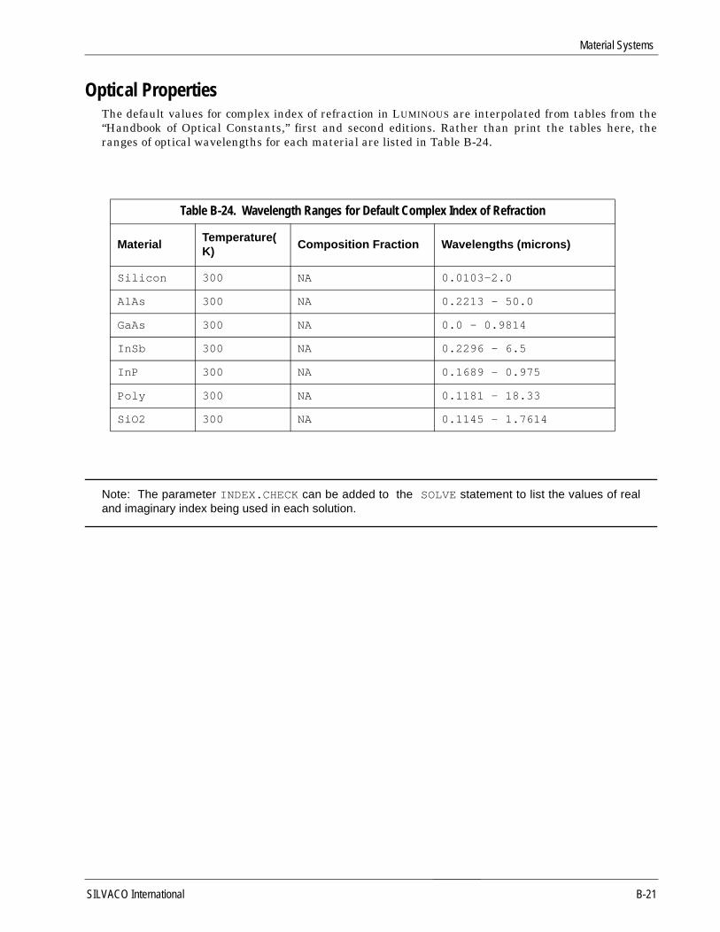
Material Systems
Optical PropertiesThe default values for complex index of refraction in LUMINOUS are interpolated from tables from the“Handbook of Optical Constants,” first and second editions. Rather than print the tables here, theranges of optical wavelengths for each material are listed in Table B-24.
Note: The parameter INDEX.CHECK can be added to the SOLVE statement to list the values of realand imaginary index being used in each solution.
Table B-24. Wavelength Ranges for Default Complex Index of Refraction
Material Temperature(K)
Composition Fraction Wavelengths (microns)
Silicon 300 NA 0.0103-2.0
AlAs 300 NA 0.2213 - 50.0
GaAs 300 NA 0.0 - 0.9814
InSb 300 NA 0.2296 - 6.5
InP 300 NA 0.1689 - 0.975
Poly 300 NA 0.1181 - 18.33
SiO2 300 NA 0.1145 - 1.7614
SILVACO International B-21
ATLAS User’s Manual - Volume 2
User Defined MaterialsThe current version of ATLAS does not directly support user defined materials. A simple workaroundcan be done using the already existing user specifications. This workaround is based on the use of analready existing material name and modifying the material parameters as appropriate.
In ATLAS material names are defined to give the user a reasonable set of default material parameters.Any of these defaults can be overriden using the MATERIAL, IMPACT, MODEL, and MOBILITYstatements. The key to defining new materials is choosing a material name that is defined in ATLAS,then modifying the material parameters of that material to match the user material. Here it is best tochoose a material that has default parameter values that might best match the user material, whilebeing sure to choose a material that is not already in the user device. Next the user must associate thismaterial name with the device regions where the new material is present. This is done by eitherspecifying the chosen material name on the appropriate REGION statements (when the device isdefined in the ATLAS syntax) or choosing the material name from the materials menu when definingthe region in DEVEDIT.
Next, the user should modify the material statements using MATERIAL, IMPACT, MOBILITY, andMODEL statements. When doing this the MATERIAL parameter of the given statement should beassigned to the chosen material name.
For materials with variations in composition fraction, the user should choose a defined material withX and/or Y composition fractions (i.e., a terniary or quaterniary material). The user may also find itconvenient to use C interpreter functions to define the material parameters as a function ofcomposition. The C interpreter functions that are useful for this approach are: F.MUNSAT,F.MUPSAT, F.BANDCOMP, F.VSATN, F.VSATP, F.RECOMB, F.INDEX, F.BGN, F.CONMUN,F.CONMUP, F.COPT, F.TAUN, F.TAUP, F.GAUN, and F.GAUP.
In defining new materials there exists a minimum set of parameters that should be defined. This setincludes bandgap (EG300), electron and hole density of states (NC300 and NV300), dielectricpermitivity (PERMITIVITY), and electron and hole mobilities (MUN and MUP). For bipolar devicescertain recombination parameters should also be defined such as: lifetimes (TAUN and TAUP), radiativerecombination rates (COPT), and Auger coefficients (AUGN and AUGP). For devices with variationsin material composition certain band-edge alignment parameters should also be defined: eitherelectron affinity (AFFINITY) or edge alignment (ALIGN). If impact ionization is considered the impactionization coefficients should also be defined.
As an example, consider the case where the user is simulating a device with an AlInGaP region.Consulting table B-1, we see that this material system is not defined in ATLAS. We then choose amateral that is defined in ATLAS which has default material parameters that best approximate thematerial parameters of the new material. In this case, we choose InGaAsP since, at least for examplepurposes, we feel that this material is closest to the AlInGaP. Next, we must specify InGaAsP as thematerial of the region(s) that is/are composed of AlInGaP. This can be done either on the REGIONstatement if the structure is defined in ATLAS syntax or from the material menu when the region isdefined in DEVEDIT.
Supposing that we are satisfied with the default values of the parameters from the "minimum set"discussed above, and that we are principally concerned with the recombination and heat flowparameters defaults, the following section of the input deck illustrates how these parameter defaultsmay be modified:
# new material AlInGaPMATERIAL MATERIAL=InGaAsP# SRHMATERIAL MATERIAL=InGaAsP TAUN0=1.1e-9 TAUP0=2.3e-8 # AugerMATERIAL MATERIAL=InGaAsP AUGN=5.8e-30 AUGP=1.1e-31# Opticalmaterial material=InGaAsP COPT=1.7e-30
B-22 SILVACO International

Material Systems
# ThermoconductivityMATERIAL MATERIAL=InGaAsP TC.A=2.49# Heat capacityMATERIAL MATERIAL=InGaAsP HC.A=1.9
SILVACO International B-23

ATLAS User’s Manual - Volume 2
B-24 SILVACO International
Appendix C:Hints and Tips
This appendix is a collection of answers to commonly asked questions about the operation of ATLAS.This information has been previously published in articles in The Simulation StandardTM, Silvaco’strade publication. The original articles can be viewed at Silvaco’s home page at http://silvaco.com/simstd.
Question:
Can ATLAS handle photogeneration from non-normally incident light? What syntax is used todetermine the correct photogeneration rate?
Answer:
The models with LUMINOUS allow simulation of photogeneration within ATLAS. Arbitrary light sourcesare available within Luminous using the BEAM statement. The program uses geometric ray tracing todetermine the path of a light beam includingrefraction and reflection of non-normally incident light. Itthen applies models for the absorption of the light to determine the photogeneration rate.
To use luminous the use should first define a light source using the BEAM statement and then choosethe light intensity using a SOLVE statement. The BEAM statement can be explained by a simpleexample. The following syntax generates the ray trace in Figure C-1.
BEAM NUM=1 X.ORIGIN=3.0 Y.ORIGIN=-5.0 ANGLE=60.0 \MIN.W=-1 MAX.W=1 WAVEL=0.6 REFLECT=2
The parameter NUM sets the beam number. LUMINOUS can applications up to 10 independent beams.X.ORIGIN and Y.ORIGIN define the initial starting point for the light beam. This must be outside thedevice coordinates and for non-normal beams it is important to keep this point well away from thedevice. The ANGLE parameter determines the direction of the light beam relative to the x-axis.ANGLE=90 gives normal incidence from the top of the device. The light is defined as coming from a lineperpendicular to the direction set by ANGLE and passing through (X.ORIGIN, Y.ORIGIN). MAX.W andMIN.W set a window along this line through which the light passes. The default for these parameters is+/- infinity.
The wavelength of the light beam is defined in microns using the WAVEL parameter. It is also possibleto specify spectral sources of light by replacing WAVEL with POWER.FILE=filename, where thefile is a UNIX text file defining the spectrum in terms of an XY list of wavelength vs intensity.
LUMINOUS automatically chooses the number of rays needed to resolve the geometry. In the case ofFigure C-1, only one initial ray is needed. The number of rays used by LUMINOUS is purely a function ofthe geometry and is not related to optical intensity, photogeneration rate, or MIN.W and MAX.W. TheREFLECT parameter is used to limit the number of reflections the light beam is allowed. In ATLASVersion 3.0.0.R an alternative parameter MIN.POWER is used to set a relative intensity below which nomore rays are traced.
The user has a choice in LUMINOUS as to whether the rays should reflect from the sidewalls and bottomof the device structure. If the simulation is of a partial wafer (such as is typical for CCD simulation)the light should not reflect. This is the default shown in Figure C-1. If the simulation is of a completedevice, such as is typical for solar cells, the light should reflect. The parameter BACK.REFL is used toenable back and side reflection. The result of adding this to the previous syntax is shown in Figure C-2. In this figure the limit set by REFLECT=2 is also clear as each ray reflects only two times.
SILVACO International C-1

ATLAS User’s Manual - Volume 2
The ray trace is only done once a SOLVE statement is used to turn on the light beam. For example, thesyntax SOLVE B1=0.5 sets the power of beam #1 to 0.5W/cm2. DC and transient ramps of lightintensity can also be performed.
The refraction and reflection are determined by the real portion of the refractive index for eachmaterial. The imaginary portion on the refractive index controls the absorption of the light.Wavelength dependent defaults exist in ATLAS for common materials, but can be defined by the user asfollows:
MATERIAL MATERIAL=Silicon REAL.INDEX=value IMAG.INDEX=value
From the ray trace information and the imaginary refractive indices, the photogeneration rate iscalculated at each node in the structure. An integration method is used to ensure the charge generatedis independent of the mesh density. The photogeneration rate from the ray trace in Figure C-2 isshown in Figure C-3. The electrons and holes generated are included in electrical simulations in ATLASto determine collection efficiency, spectral response and other device parameters.
Figure C-1: Simple ray trace in LUMINOUS
Figure C-2: Addition of back and sidewall reflection to Figure C-1
C-2 SILVACO International

Hints and Tips
Figure C-3: Photogeneration contours based on ray trace in Figure C-2
Question:
What choices of numerical methods are available in ATLAS? When should each type of method be used?
Answer:
The latest release of ATLAS features more choices of numerical methods for users. It also has a newmore logical syntax that clears up some of the previously confusing issues with the choice of numericalmethod for ATLAS solutions.
ATLAS has the ability to solve up to six equations on the simulation mesh. These are the Poissonequation, two carrier continuity equations, two carrier energy balance equations, and the lattice heatflow equation. The choice of numerical technique in solving these equations can strongly affect boththe convergence and CPU time required to complete a simulation run.
In general equations can either be solved in a coupled manner with all equations solved at once or adecoupled manner with a subset of the equation solved whilst others are held constant. The coupledsolutions are best when the interactions between the equations is strong (i.e., high current producingsignificant local heating). However they require a good initial guess to the solution variables forreliable convergence. Unless special techniques, such as projection, are used for calculating initialguesses this would mean that the voltage step size during a bias ramp might have to be rather small.
Decoupled methods can have advantages when the interaction between the equations is small(typically low current and voltage levels). They do not require such good initial guesses forconvergence. They tend to either not converge or take excessive CPU time once the interactionsbecome stronger.
ATLAS uses the METHOD only statement to define numerical methods. The older SYMBOLIC statement isno longer required, although existing input files will run as before. To select the decoupled method fortwo carriers use:
method gummel carriers=2
To select the coupled method for two carriers use:
method newton carriers=2
SILVACO International C-3

ATLAS User’s Manual - Volume 2
This is the default. In fact users do not need to specify a METHOD statement at all for this case. For themajority of isothermal drift-diffusion simulations this choice of numerics is the recommended one.
ATLAS has the ability to switch automatically between different numerical methods. The syntax
method gummel newton
would start each bias point using a decoupled method and then switch to a coupled solution. Thistechnique is extremely useful when the initial guess is not good. Typically this happens for deviceswith floating body effects (i.e., SOI).
For more complex simulation with energy balance or lattice heating other techniques are alsoavailable in ATLAS. A mixed technique where the poisson and continuity equations are solved coupled,and then the other equations are decoupled can be applied.
The syntax for this is:
method block
Typically this mixed technique is quicker and more robust at low lattice and carrier temperatures,whereas the fully coupled technique is better for high lattice and carrier temperatures. The mixedmethod can be combined very effectively with the fully coupled technique to provide improved speedand convergence for all ranges using:
method block newton
As an example of this Figure C-4 shows the CPU time taken for individual biasing points for a non-isothermal energy balance simulation of second breakdown of a sub-micron MOSFET. The device wasconstructed using ATHENA and the mesh contains a low number of obtuse triangles (not zero). Thegraph clearly shows that at initially the coupled method takes much longer to converge. This isbecause the initial guess is not good until two bias points are solved so that projection can be used. Asthe voltage is increased the block method has increasing convergence difficulty whereas the timetaken for the newton method is flat. The time for the mixed method has the advantages of block atlower currents, but without the severe increases of block.
The ideal solution for most problems is the use of the mixed "block newton" method initially switchingto the fully coupled "newton" method as the simulation proceeds. Of course the cross-over point, whichis at x=2.5 in Figure C-4, varies from case to case. To avoid excessive user-interaction the "blocknewton" could be used throughout the simulation without a very excessive hit in terms of CPU time.
Figure C-4: Comparison of CPU time showing advantages of decoupled methods at low current and coupled method at high currents
C-4 SILVACO International

Hints and Tips
Question:
Can the workfunction of the MOS polysilicon gate contact be calculated by ATLAS based on the doping?Can poly depletion effects be simulated in ATLAS?
Answer:
The polysilicon gate contact in MOS devices can be simulated in two distinct ways using ATLAS. Thesecorrespond to treating the polysilicon region as:
• A metal-like equipotential region with a specified workfunction.
• A semiconductor region with a potential defined by the doping level.
Most commonly the former approach is adopted. The polysilicon region acting as the gate is defined asan electrode in ATHENA.
The electrode statement is used with the X and Y parameters acting as crosshairs to target aparticular region of the structure. The whole region, irrespective of shape, is then defined as anelectrode.
ELECTRODE NAME=gate X=x value Y=y value
A region defined this way is now treated as equipotential in ATLAS. The potential of this region will bedefined by the VGATE parameter of the SOLVE statement. Hence poly depletion cannot be modeled ingate contacts defined this way. The workfunction of this region must be set by the user. For example, aheavily n doped polysilicon contact can be defined by either of the two following statements:
CONTACT NAME=gate N.POLY CONTACT NAME=gate WORK=4.17
The second approach of treating the polysilicon gate region as a semiconductor is achieved by placing acontact on the top of the gate. In ATHENA this is done be depositing a metal (or silicide) layer on top ofthe polysilicon. The ELECTRODE statement is then used to define this metal region as the gateelectrode. In ATLAS a workfunction for the gate should not be specified on the CONTACT statement asthis would give an undesirable workfunction difference between the metal and polysilicon. thepotential on the metal region is defined by the VGATE parameter of the SOLVE statement. The potentialwithin the polysilicon gate region will depend on the doping level of the polysilicon. In non-degenerately doped polysilicon a voltage drop is seen across this region from top to bottom. Theworkfunction difference between the gate and the substrate can be derived from a potential profilethrough the channel region.
It is also possible for the polysilicon to be depleted starting at the gate oxide interface. Figure C-5shows a comparison of high frequency CV curves between a MOS device with a uniform degeneratelydoped poly gate typical when tube doping is used and a lighter, non-uniformly doped gate typical whensource/drain implants are used to dope the polysilicon. In the accumulation region the poly begins todeplete leading to an effectively thicker gate dielectric. This effect is illustrated in Figure C-6. Theamount of poly depletion observed is dependent on the doping level. Accurate polysilicon diffusionmodels are available in ATHENA to simulate the doping. In addition the SILICIDE module allowssimulation of the dopant redistribution during gate silicidation. Silicides can typically reduce theeffective gate doping making poly depletion more likely.
SILVACO International C-5

ATLAS User’s Manual - Volume 2
Figure C-5: High frequency CV curve showing poly depletion effects at positive Vgs.
Figure C-6: Figure 2 Electron concentration profile of an NMOS transistor poly depletion occurs at the poly/gate oxide interface.
C-6 SILVACO International

Hints and Tips
Question:
How can I remesh my process simulation result for device simulation?
Answer:
The structure editing and griding tool DEVEDIT provides an effective way to remesh structures betweenprocess and device simulation.
DEVEDIT is able to read and write files to both ATHENA and ATLAS. In addition to the graphical userinterface, DEVEDIT can operate in batch mode under DECKBUILD. The batch mode DEVEDIT features apowerful syntax that can be applied to remesh structures read directly from ATHENA. DEVEDIT employsa heirachical method for remeshing existing structures. Users specify mesh parameters at each stage.Initially a base mesh is applied with the command:
BASE.MESH HEIGHT=<h1> WIDTH=<w1>
This mesh of h1 by w1 microns provides the coarsest mesh in the structure. On top of this base levelmesh DEVEDIT determines which points must be added to ensure the geometry of all regions ispreserved. Optional boundary conditioning to smooth region boundaries can be applied using theBOUND.COND statement.
Mesh constraints can be applied to arbitrary boxes with the device using the syntax:
constr.mesh x1=<n> x2=<n> y1=<n> y2=<n>\max.height=<h2> max.width=<w2>
This sets the maximum mesh size to h2 by w2 microns the box with diagonal from (x1,y1) to (x2,y2).Using the constraint boxes in critical areas of the device is the most effective way to use DEVEDIT. InMOSFETS the constraint boxes can be applied to the silicon region under the gate. Typically verticalgrid spacings of 5 are required for accurate simulation of channel conduction in sub-micron MOSFETs.
Use of multiple constraint boxes can be applied. For MOSFET breakdown constraint boxes can beapplied to the drain/gate overlap area.
In addition to constraint boxes, DEVEDIT can refine on quantities such as individual doping species, netdoping, potential. The IMP.REFINE statement allows users to select the critical value of a quantity forrefinement and an associated minimum grid spacing.
This type of refinement is useful when key effects are located very close to junctions. For example theemitter-base junction in bipolar transistors.
The final level of grid refinement are "manual refine boxes" defined using:
Refine Mode=Both|x|y P1=x1,y1 P2=x2,y2
These are boxes with a diagonal from (x1,y1) to (x2,y2), inside which the grid spacing is halved in thegiven direction. These can be used as a final customization to the mesh. In general, however, theconstraint boxes described above are easier to use.
As a demonstration of the effectiveness of regriding using devedit Figures C-7 and C-8 show meshescreated from the same process simulation structure. Figures C-9 and C-10 show the Id/Vds andbreakdown characteristics respectively of the device for each mesh. The mesh at the silicon surface isidentical in both cases to a depth of 100A. However the mesh below this is much coarser in Figure C-8.
However the device results show no significant change despite the reduction in the node count by afactor of two.
SILVACO International C-7

ATLAS User’s Manual - Volume 2
Figure C-7: Fine Grid - 5000 nodes
Figure C-8: Fine Grid only in Key Areas - 2450 nodes
C-8 SILVACO International

Hints and Tips
Figure C-9: Id-Vds Curves for two MOSFET Meshes
Figure C-10: Breakdown Voltage for Two MOSFET Meshes
Demonstration of optimized griding using constraint boxes in DEVEDIT. Both very fine and optimizedmesh produces equivalent results.
SILVACO International C-9
ATLAS User’s Manual - Volume 2
Question:
How can solution quantities such as Electric Field be saved for plotting against applied bias?
Answer:
There are two types of output files saved by ATLAS:
• Solution files contain physical quantities mapped to the simulation grid. One solution file is saved per bias point.
• Log files which traditionally have saved the terminal characteristics for all bias points.
A new feature of ATLAS 4.0 is the addition of a capability to save physical quantities at user-specifiedlocations within the device grid to the log files. A new statement PROBE is used to specify the quantityto be saved and the location. For example, to save the electron concentration rate at a location [1,0.1]the syntax is:
PROBE NAME=my_e_conc N.CONC X=1.0 Y=0.5
The label specified by the NAME parameter is used to label the saved quantity in TONYPLOT andsubsequent EXTRACT statements.
For vector quantities the PROBE statement also requires a direction to be given using the DIRparameter. This is specified as an angle in degrees with the X axis as DIR=0. To find the electric fieldacross an oxide layer the syntax is:
PROBE X=1.2 Y=0.2 FIELD DIR=90 \ NAME=oxide_field
Figure C-11 shows the resultant plot of electric field in a MOSFET gate oxide during a transient ESDpulse. This result shows the probability of oxide breakdown during the ESD stress, without the need toexamine many separate solution files.
Another advantage of the probe for vector quantities is that it reads the values directly from thesimulator at the closest location to the specified XY coordinates. This avoids many issues ofinterpolation and averaging of vector quantities onto the simulation grid.
If two physical quantities are probed at the same location it is possible to plot them against each otherto examine model settings. For example, impact ionization rate or mobility versus electric field. FigureC-12 shows a plot of channel electron mobility in a submicron NMOS transistor versus the transverseelectric field from the gate.
All of the primary solution quantities can be probed. A full list is given in the manual under thePROBE statement. In addition to values at point locations the PROBE statement also supports MINand MAX parameters to find the minimum and maximum of a given quantity.
C-10 SILVACO International

Hints and Tips
Figure C-11: Electric field in MOS gate oxide during a high current pulse on the drain.
Figure C-12: Mobility (normalized) rolls off as a high gate electric field is applied
SILVACO International C-11

ATLAS User’s Manual - Volume 2
Figure C-13: Using a PROBE of electron concentration allows a study of MOS width effect using 2D simulation. An enhanced electron concentration is seen along slice 2.
Question:
What are the options for generating 3D structures for ATLAS device simulation?
Answer:
Currently there are three options for generating 3D device structures. In all cases the prismaticmeshing of ATLAS/DEVICE3D permits arbitrary shaped device regions in 2 dimensions (typically X andY) and rectangular regions in the other dimension (typically Z).
• Definition though the ATLAS syntax.
This limits the user to defining box shaped regions. Region definition is though statements such as:
region num=1 silicon x.min=0 \ x.max=1 y.min=0 y.max=1 z.min=0 \ z.max=1
Mesh generation is handled though the Z.MESH statement which is analogous to the X.MESH andY.MESH statement used in 2D ATLAS simulations. Electrodes and doping can be defined using the samesyntax as 2D ATLAS but with Z.MIN and Z.MAX parameters to control the Z extent. Doping profiles canbe read from the formats supported in 2D ATLAS: ssuprem3, athena, ascii.
• Use DEVEDIT to create a 3D mesh structure.
DEVEDIT3D is a 3D structure generation and meshing tool used to generate the mesh, regions,electrodes and doping used in ATLAS/DEVEDIT. It allows users to draw regions by hand in 2D andproject them into the third direction.
DEVEDIT3D contains all the sophisticated meshing options available to 2D DEVEDIT. These include:mesh constraints by region, mesh constraints by a user defined box, refinement on doping and other
C-12 SILVACO International

Hints and Tips
quantities, mouse controlled refine and unrefine boxes. DEVEDIT3D has both interactive and batchmode operation. This is the recommended approach for 3D power device simulation.
• Use ATHENA and DEVEDIT3D to extend a 2D process simulation to 3D.
A 2D process simulation from ATHENA can be extruded to form a 3D structure using DEVEDIT3D. In thismode DEVEDIT3D can be used to add extra regions and doping if required. This mode us commonly usedfor modeling MOS width effects in 3D (see Figure C-14). An ATHENA simulation of the isolation bird'sbeak and field stop implant is performed.
The 2D structure is loaded into DEVEDIT3D and extended in Z direction. The polysilicon gate istruncated in Z and aluminum source/drain contacts are added. The source/drain doping profiles can beread from analytical functions or other process simulation results. A worked example, namedmos2ex04.in, is supplied with the Fall 96 release CDROM.
Figure C-14: 3D device simulation of MOS width effect can be performed on structures created ATHENA.
For devices with non-rectangular regions in the XZ plane such as pillar MOSFETs or cylindricallydesigned power structures DEVEDIT3D can also be used by drawing in the XZ plane and projecting intothe Y direction.
The future release of Silvaco's 3D process/device simulator ODIN will provide a fourth option for 3Dsimulation problems. ODIN is based on tetrahedral mesh elements and will overcome the meshrestrictions described above.
SILVACO International C-13

ATLAS User’s Manual - Volume 2
[This page intentionally left blank]
C-14 SILVACO International
Appendix D:ATLAS Version History
Version History
Version 5.2.0.R1. Introduced LUMINOUS3D
• LUMINOUS3D provides a similar functionality to 2D LUMINOUS. This allows simulationof interaction between arbitrary optical sources and semiconductor devices in threedimensions.
2. Smartlib
• Implemented the SmartSpice Compact Device Model Library (Smartlib). These modelsreplaces the old MIXEDMODE Diode, MOSFET and BJT Models. Additional device modelssuch as TFT and SOI can now be used. Also, additional devices such as JFETS andMESFETs can now be used.
3. Implemented a New and Improved C-Interpreter
• Implemented a new C-Intrepreter. This completely replaces the old version of the C-Interpreter. The new C-Interpreter is faster than the old version and supports more Cfunctions. The new C-Interpreter conforms more to the ANSI standard.
4. Hetereojunction Thermionic Emission and Field Emission
• Introduced a new implementation of thermionic emission models for hetero-interfaces. Thisimplementation supercedes the previous one, which is no longer supported.
• Also introduced a new heterojunction tunneling (thermionic field emission) model that iscompatible with the new thermionic emission model.
5. Cyclic Biasing
• Implemented cyclic biasing model to simplify prediction of steady state conditions incyclically biased devices exhibiting long time constants.
6. Miscellaneous Improvements
• Added the following new material names: InGaN, AlGaN, InAlGaN, inganas, InGaNAs,inGaNP, AlGaNAs, AlGaNP, A1InNAs, AlInNP, InA1GaAs, InA1GaP and InA1AsP.
• Added the following new gain output parameters. ATLAS will now ouput the maximumavailable gain (Bma) as well as the maximum stable gain (Gms).
• Added capability to add sheet charge along region interfaces for simulation of piezoelectricstrain effects.
• Added temperature dependence to the Shirahata mobility model.
• Added capability for multiple trapazodial/square transient pulses.
• Added a more general parameterized temperature-dependent model for saturation velocityfor field-dependent mobility.
• Changed the calculation of effective mass used in calculation of thermal velocity for traps innoo-silicon materials. The new approach calculates mass, based on the material density ofstates.
SILVACO International D-1

ATLAS User’s Manual – Volume 2
Version 5.0.0.R
1. Introduced several new 3D products
a. Giga3D.
• Giga3D contains most of the functionality of the 2D Giga, but works with 3D products. Thisallows modeling of heatflow and self-heating effects in 3D devices. The only functionality notsupported in this version of Giga3D that is supported in 2D is the BLOCK method.
b. Blaze3D
• This version accounts for spatial variations in band gap due to spatial variations in materialcomposition in 3D. This version supports all the same models that are supported in Blaze 2Dwith the exception of thermionic emission at hetereojunctions and energy transport. Thisversion also does not support compositional variation in the z direction.
c. MixedMode3D
• This improvement allows simulation of 3D devices embedded in lumped element circuits.MixedMode3D contains all the functionality of 2D MixedMode simulator.
d. TFT3D
• This model allows modeling of poly and amorphous semiconductor devices such as TFTs in3D. This model has all the functionality of the 2D TFT simulator.
e. Quantum3D
• This allows modeling of the effects of quantum confinement using the quantum momentapproach. This model has all the functionality of the 2D Quantum model.
2. Orchid
• Orchid is a new product used in conjunction with SPisces to model the effects of totalradiation dosage on MOS device reliability. Key to this capability is the ability to model the gateoxide as a semiconductor. The user may then define carrier pair generation in the oxide as afunction of position, time, and electric fields, using a new C interpreter function. Another Cinterpreter function can be used to calculate the cumulative fixed charge density as a functionof position and electron and hole current densities in the oxide. The deduced fixed oxide chargedensity directly effects the threshold degradation of the device.
3. Introduced SiC
• SiC is a new simulation capability for simulating anisotropic materials such as silicon carbide.The basis of this model is the incorporation of a new anisotropic mobility model that allowsusers to define separate mobilities along normal directions.
• Also added a new default value for thermal conductivity and electron saturation velocity ofsilicon carbide.
4. Modifications to Laser
Included additional functionality into Laser. The new features are:
• transient mode (time-dependent photon rate equation)
• far field patterns
• addtitional loss mechanisms including:
– mirror loss
– free carrier loss
– absorption loss (including C interpreter function for bulk absorption)
5. New Large Lignal and Simulation Capabilities
• Added specifications of sinusoidal waveforms to the SOLVE statement.
• Implemented post processing Fourier analysis. This performs a Fast Fourier Transform (FFT)on data within a log file to convert time domain data into frequency domain data.
D-2 SILVACO International

ATLAS Version History
• Added solution compliance based on sinusoidal analysis. In this mode, transient simulationwill stop if the amplitude of a sinusoidal waveform is less than the user-specified value.
6. Modifications to LUMINOUS
• Added capability to print the complex indices of refraction as they are calculated for the variousmaterials during the ray trace in Luminous.
• Added functionality to simulate single-layer antireflective coatings in Luminous. Thiscapability calculates the reflection coefficient for a single layer coating under conditions ofnormal incidence.
7. Modifications to MIXEDMODE
• Added the capability to specify multiple .TRAN statements in a single input deck.
Added the extraction of network parameters (S, Z, Y, H, ABCD), stability factor, unilateral powergain, and maximum unilateral transducer power gain in MIXEDMODE.
• Added the capability to use the PROBE in MIXEDMODE.
8. Modification to GIGA
• Enabled simulations of floating gate structures with heat flow in GIGA.
9. New Physical models
• Added Klaassen’s concentration and temperature-dependent SRH lifetime and Auger ratemodels.
• Implemented new continuous trap level model in TFT.
• Added new carrier concentration dependent Auger coefficient model.
• Added the capability to calculate the band-to-band tunneling coeffiicients from principles.
• Added the capability to model thermionic field emission tunneling in Schottky contacts.
• Added two new parameters to the single-event upset model. The generated electron/holes pairs(or charge) will not be calculated after tf seconds if this parameter is specified in the inputdeck. The width of the beam can now be specified as a constant value, followed by anexponential or Gaussian function by using the beam.radius parameter. For radi greater thanbeam.radius, either the Gaussian or exponential functions is used (if they are specified).
10. New Numerical Techniques
• Two sparse matrix reordering techniques are now available: Minimum Degree (MD) andReverse Cuthill McKee (RCM). They are used in the 2D linear solver. MD is the default.Choosing RCM instead of MD sometimes solves the problem of having a zero on the diagonal,which is indicated by the error message:
Internal error in linear solver: Z-#.
If this happens, the user should switch from MD to RCM or vice-versa.
• For Parallel ATLAS, two new mesh partitioning techniques are now available:
– Natural Ordering (NO) and
– Multi-level Graph Partitioning (MGP)
These are used to assign sub-meshes to different processor. MGP is the default and should alwaysoutperform NO. On the other hand, NO requires less preprocessing time and might perform aswell as MGP in the case of meshes generated by the ATLAS statement.
• Made it possible to use projection for initial guesses in conjunction with current boundaries.
11. Structures and Log File Improvements
• Added the capability to write X and G (rhs) errors in a standard structure file for subsequentvisualization using TONYPLOT.
• Added the capability to save electron, hole relaxation times, and Peltier coefficients to
SILVACO International D-3

ATLAS User’s Manual – Volume 2
structure files.
• Added the capability to save electron, hole, and displacement currents to log files.
12. New Quantum models.
• Implemented a new self-consistent Schrodinger-Poisson solver. This model interactively solvesPoisson’s and Schrodinger’s equations to calculate the potential and carrier concentration,including the effects of quantum confinement. These solutions also produce eigen energies andeigen functions.
• Added Hansch’s model for quantum mechanical correction for carrier distributions in Nchannel MOSFETs inversion layers.
• Added van Dort’s model for quantum mechanical correction for carrier distributions in N and Pchannel MOSFETs in inversion and accumulation layers.
13. Miscellaneous ATLAS Improvements
• Reconfigured small signal AC post processing to include the effects of parasitics in gaincalculations.
• Changed functionality of C interpreter functions, F.CONMUN and F.CONMUP, to account fordonor and acceptor concentrations separately.
• Added trap concentrations to concentration-dependent mobility models and band gapnarrowing models.
• Added new C interpreter functions for energy-dependent relaxation times for electrons andholes.
• Added new C interpreter functions for energy-dependent Peltier coefficients for electrons andholes.
• Added a new C interpreter function to specify doping in 3D as a function of position.
• Added extra checking to the AC memory allocation. If there is insufficient memory for thefactorization, more will be allocated. A warning message will also be printed.
• Enabled multiple contacts with the same name to have the same work function and otherparameters.
• Modified the DOPING statement so that ATHENA master files can now be used in 2D.ATHENA doping is interpolated onto the ATLAS mesh.
Version 4.3.0.R1. Introduced Quantum Transport Model
This model accounts for redistribution of carriers near abrupt material transitions due to the effects ofquantum confinement. It is also useful when simulating heterojunction devices such as HBTs andHEMTs, as well as short channel thin gate oxide MOS devices.
2. Introduced Improvements to the Ferroelectric Model
This release includes modifications which allow better modeling of unsaturated loop simulation offerroelectric materials. It also includes the capability to characterize the AC ferroelectric permitibityaffected by the polarization as a fraction of the DC case.
3. Log File Improvements have been Made for Capturing Data
• PROBE has been enhanced to add the capability of probing minimums and maximums of thedirectional quantities; electric field, electron mobility, hole mobility and polarization.
• PROBE has been enhanced to allow the measurement of dielectric permitivity and the band-to-band tunneling rate.
• Added the capability to capture simulation time in the log file.
D-4 SILVACO International

ATLAS Version History
4. Structure File Improvements
The default method of averaging for capture of impact ionization rate, the electron and hole mobilitiesto the structure file has been changed. The new averaging techniques provide smoother plots inTonyPlot.
5. Improved Parameterization of Band-to-Band Tunneling Models.
This release allows user accessibility to the gamma parameter of the standard band-to-band tunnelingmodel.
Version 4.0.0.R
1. Introduced a ferroelectric permitivity model
This model accounts for ferroelectric polarization and hysteresis. This release includes a new model tomodel ferroelectric materials. It is useful for simulating ferroelectric devices such as ferroelectriccapacitors and FETs.
2. Introduced Klaassen’s mobility model
This release includes a new model for low field electron and hole mobilities in silicon. This modelaccounts for lattice, impurity, and carrier scattering and screening as a function of temperature,doping and carrier concentrations. This model has been calibrated over a wide range of conditions andshould be used as the default low field model for silicon simulations.
3. Introduced Concannon’s gate and substrate current models
This release includes a new model for EPROM simulation. This model estimates the gate current inEPROM devices as a function of carrier temperature by integrating a non-maxwellian distributionfunction. The model also uses a impact ionization model that uses the same distribution function toensure a direct relationship between gate and substrate currents.
4. Introduced Shirahata’s mobility model
This release includes a new surface mobility model which accounts for carrier screening effects in thechannel. This is done largely by using Klaassen’s model for the low field mobility. The model alsoaccounts for parallel and perpendicular fields in the channel.
5. Introduced a "Probe" capability
A new statement has been implemented which allows users to write local scalar quantities (e.g.potential, electron concentration, hole concentration, etc.) and vectors (e.g. field etc.) to the log file as afunction of bias, time etc. The user may specify the probe by location, minimum or maximum, andtype.
6. Modifications to the Watt mobility model
Several modifications were made to the Watt mobility model. First, the user may now apply the modelto grid nodes below the interface down to a user specified depth. Also the user can use an exponentialscaling on the effective field. Finally, the user can make the models only apply to minority carriers.
7. Improved vector averaging
Certain quantities used in ATLAS are not defined on grid points but between points (e.g. electricfields). To write these quantities into the structure files they must be averaged. In thisimplementation an improved averaging scheme was introduced which produces smoother results. Theuser also has control over various weighting schemes for the averaging.
8. Traps in MIXEDMODE
New parameters were introduced to the TRAP, INTTRAP, DEFECT, and INTERFACE statements toenable proper handling of these physical models in MIXEDMODE.
SILVACO International D-5

ATLAS User’s Manual – Volume 2
9. Modified run time outpu
The ATLAS run time output was modified to be more concise and informative.
10. Misalignment and delta CD in INTERCONNECT3D
INTERCONNECT3D now allows users to specify misalignment and variations in critical dimensionswith interconnects specified by mask sets from MASKVIEWS.
11. Lumped elements and current boundary conditions in DEVICE3D
DEVICE3D now supports lumped element and current boundary conditions.
12. GaAs in DEVICE3D
DEVICE3D now supports GaAs material models.
13. Electric field lines.
Electric field lines can now be plotted in TONYPLOT. The specification of where to elines lines arecalculated was improved for both plotting and for evaluation of ionization integrals.
14. Energy dependent impact ionization coefficients.
Two new C interpreter functions were introduced to enable user specification of impact ionizationcoefficients as a function of carrier temperature for Selberherr’s model.
15. Removed obsolete syntax
The FIT, COLOR, CONTOUR, LABEL, LOOP, L.END, PLOT.1D, PLOT.2D and PLOT.3dstatements are no longer supported by ATLAS. Equivalent functionalities are available throughDECKBUILD and TONYPLOT.
16. DEVICE3D improvements for SEU simulation
Introduced a new C interpreter function, F3.RADIATE. This function allows users to specify arbitrarygeneration rate versus spatial position and time. The SINGLEEVENTUPSET statement was changed toallow users to control whether the generation rate is scaled by the ratio of the numerical and analyticintegrals of the analytic generation function. This permits conservation of total generation rate in adevice. By default the rescaling is now turned off.
17. MIXEDMODE Improvements
The .DC statement now allows linear and logarithmic stepping of sources and nested sweeps.
Version 3.0.0.R
1. First release of “six equation solver” version of ATLAS.
In this release an advanced Non-Isothermal Energy Balance Model was implemented. The modelallows self-consistent solution of a set of up to 6 partial differential equations for electrostaticpotential, electron and hole concentrations, electron and hole carrier temperatures, and latticetemperature. All the important combinations of equations are supported.
2. DEVICE3D introduced.
DEVICE3D is introduced as the first truly 3D simulator in the ATLAS framework. It is a virtualanalogy to S-PISCES. With it three dimensional steady-state silicon device simulation can beperformed to calculate electrical behavior of bipolar and MOS transistors, as well as EPROM devices.
• Syntactically and behaviorally like ATLAS S-PISCES.
• Poisson, one carrier or two carrier analysis can be performed.
• Uses Gummel, Newton or combined Gummel/Newton algorithms.
• Supports semi-implicit scheme for transient simulation. Significantly faster than TR-BDF.
D-6 SILVACO International

ATLAS Version History
• Supports the essential set of physical models for silicon modeling including: SRHrecombination,
Auger recombination and radiative recombination; concentration dependent mobility models(Conmob,Arora, Analytical); longitudinal and transverse electric field dependent mobility models(Caughey-Thomas, CVT, Yamaguchi); Band Gap Narrowing (BGN), Boltzman statistics, Fermi-Diracstatistics, and incomplete ionization; Fowler-Nordheim current calculation, Lucky electron model forhot carrier injection and transient programming and erasing of EPROM devices.
• The three dimensional simulated structure can be specified using DEVEDIT3D.
• Uses TONYPLOT3D for postprocessing.
• Single Event Upset simulation is feasible with DEVICE3D. The capability of single eventupset/ photogeneration transient simulation has been introduced. It allows specification ofmultiple tracks and radial, length and time dependence specification of generated charge alongtracks.
3. THERMAL3D introduced.
THERMAL3D is introduced as a new capability for three dimensional simulation using ATLAS. ThePoisson equation for temperature is solved in three dimensional regions of specified heat conductivitywith defined temperatures on thermal contacts (which are ideal heat conductors). The user mayspecify the thermal properties of regions heat sources, and heat sinks.
• Four models of temperature dependent thermal conductivity.
• User may specify independent temperatures on all thermal sinks (thermal electrodes).
• User may specify multiple independent heat sources.
• Completely compatible with ATLAS.
• The simulated structure is specified using DEVEDIT3D (including thermal electrodes).
• Temperature distributions can be examined using TONYPLOT3D.
4. INTERCONNECT3D introduced
INTERCONNECT3D has been introduced as another 3D capability in the ATLAS framework. Thissimulator is used to extract parasitics from arbitrary 3D interconnect structures.
• Can extract parasitic capacitance and conductance for arbitrary 3D interconnect structures.
• Provides an interface to MASKVIEWS for simple mask layer definition of interconnect structure.
• Completely compatible with ATLAS.
5. Curve tracer introduced
Allows automatic tracing of complex IV behavior (including functions that are multivalued) withoutuser intervention. Automatically varies an external resistance on a given contact to ensure optimalsteps are chosen.
6. Enhancements for Energy Balance Model
Aside from the introduction of the “Six Equation Solver”, several other improvements were made withrespect to the Energy Balance Model (EBM).
• Fermi statistics can be used with the EBM.
• The “GaAs” like mobility model can be used with the EBM.
• The energy relaxation length can be specified for impact ionization in the EBM.
• Carrier temperature projection for initial guesses is supported.
7. New solution methods
8. GIGA improvements
Aside from the introduction of the “Six Equation Solver”, several other enhancements were made toGIGA.
SILVACO International D-7

ATLAS User’s Manual – Volume 2
• GIGA now allows self consistent 5 and 6 equation solutions of lattice temperature with electronand hole temperatures.
• GIGA now supports static projection for initial guesses for lattice temperature.
9. LUMINOUS improvements
In this release many improvements were made to LUMINOUS.
• LUMINOUS now supports extraction of spatial response to optical sources.
• A MIN.POWER parameter of the BEAM statement can now be used to limit the number of raystraced in LUMINOUS.
• LUMINOUS now recognizes metals (electrodes) as bulk regions.
• Optical properties of bulk metal (electrodes) region can now be defined.
• The C Interpreter function RADIATE for user definable photogeneration was enhanced toinclude time dependence.
10. TFT improvements
Several enhancements were made in this release for TFT.
• Parameters were introduced to allow control of the number of mid-gap states used for TFTsimulations.
• TFT now supports output of donor and acceptor trap state densities and energies to userspecifiable files for examination by TONYPLOT.
• TFT now provides two new Interpreter functions for specifying the donor and acceptor densitiesas a function of energy.
11. Miscellaneous new features
A host of new features were introduced into ATLAS in general.
ATLAS now properly handles touching electrodes and electrodes with the same name.
Incorporated the trap assisted tunneling model given in Hurkx, G.A.M., Klassen, D.B.M. and Knuvers,M.P.G., “A New Recombination Model for Device Simulation Including Tunneling”, IEEE Transactionson Electron Devices, V. 39, No. 2. Feb., 1992, pp. 331-338. This model accounts for tunneling via traptransitions using an analytic approximation that modifies the lifetimes in the standard Schockley-Read-Hall recombination model.
Modified the models for hot electrons, and holes and Fowler Nordheim tunneling currents. The newmodels account for the flow of the electrons/holes in the insulating layers to arbitrary electrodes basedon one of two primitive models. The first, is the default model and trys to force the currents to followthe maximum potential gradients to find the proper electrode. In the second model insulator, currentsgo the the nearest electrode. With these modifications the electrode current run time outputs aremodified to better reflect the new models.
Enabled correct small signal simulation when simulating with bulk and interface traps.
Distinction made between active and chemical dopant densities.
Small signal analysis with interface traps now works properly.
Moved the C Interpreter function F.COMPOSIT from the MATERIAL statement to the DOPINGstatement. In previous releases this function did not work as advertised, since material compositionneeded to be defined at structure creation. In order to make the function work properly it had to bemoved to the DOPING statement.
In addition to CLIMIT parameter which existed earlier, new parameters CLIM.DD and CLIM.EB wereadded in METHOD statement. CLIM.DD is exact analog of CLIMIT parameter, but in comparisonwith CLIMIT it specifies dimensional value of minimal concentration which can be resolve usingATLAS. By default CLIM.DD is not specified and ATLAS uses default value of CLIMIT, as in previousversions. Parameter CLIM.EB can be treated as regularization parameter for the case of very smallelectron (hole) concentration for energy balance model. It specifies the mimimal value of concentrationfor which relaxation term in energy balance equation will be still properly resolved, otherwise
D-8 SILVACO International

ATLAS Version History
temperature for the points where concentration is much less than CLIM.EB, will tend to latticetemperature.
12. New syntax
With this release, the ATLAS syntax was augmented to simplify and somewhat rationalize some of themore confusing problems.
• The SYMBOLIC statement is no longer needed.
• The numerical method can now be specified on the MODEL statement. The user may choosefrom Gummel, Block and Newton methods. More than one method can be chosen; and ATLASprovides automatic switching between the methods.
• ATLAS now supports a new syntax for specifying which equations are simulated. The syntax isnow supported on either the MODEL or METHOD statement and is the preferred syntax forfuture compatibility. The new syntax provides a more rational, intuitive way of choosing whichequations are solved.
• ATLAS still supports syntax from previous versions.
13. Improved run-time output
Many improvements have been made to the run-time outputs of ATLAS.
• Added multiple levels of verbosity.
• Improved printing of mesh statistics, region and electrode summaries and models.
• Printing of error messages was made more consistent and informative in many places inATLAS.
• Removed spurious printout from S parameter extraction with the UTMOST statement.
14. New platforms
ATLAS has now been ported to DEC Alpha and SGI workstations.
15. Miscellaneous bug fixes
In this release many bugs were removed that existed in the previous version.
• Fixed bug that caused setting the value of the MODEL statement parameter CCS.EA to alsoset the value of the MATERIAL statement parameter COPTR.
• Fixed bug causing improper association of nodes with regions on BLAZE structures read infrom DevEdit. In some instances nodes j would be assigned a region at the interface then thecomposition fraction (e.g.) from the opposing region, thus causing distortions in the banddiagram at the interface.
• Fixed bug in static projection. Bug caused by two consecutive bias steps of opposite polarity.
• Fixed bug in TFT. Caused the midgap Gaussian donor defects to have the same distribution asthe midgap acceptor defects.
• Fixed bug in UTMOST interface. Bug caused ATLAS not to recognize routines 2, 3, 5, 12, 13,14, and 26.
• The calculations for the electron and hole mobilities in the InGaAsP system were found to be inerror both in the manual as well as the code. Referring to the ATLAS Users manual, Edition 2,in the equations B-36 and B-37, the “y”s should be replaced by (1-y). This fix was introducedinto the code for this release.
• Fixed a bug in the calculation of electric fields for output to structure files for examination inTONYPLOT. This bug caused the estimates of the X and Y components of the electric field to becalculated based on the dielectric constant of silicon for all semiconductors. Although, thecalculation properly handled insulators it used the dielectric constant of silicon for allsemiconductors regardless of composition. This has been fixed in this version.
Fixed bug causing extra space in UTMOST format output log files.
SILVACO International D-9

ATLAS User’s Manual – Volume 2
16. New examples
In this release the standard examples were completely reworked and improved. The ATLAS examplesare now divided into 21 application specific areas. There are now 117 ATLAS examples in all whichillustrate virtually all the functionality of ATLAS.
17. Improved quality control
In this version, new quality control tools and procedures for automated testing were implemented andused that greatly simplify and expanded ATLAS testing. This version of ATLAS represents the mostthoroughly tested version to date. Continued application of the improved quality control procedureswill ensure that future versions will continue to be of the highest quality.
Version 2.0.0.R 1. Improved Standard Structure Output – The standard structure output format has been
improved to account for multiple values at region interfaces (e.g., contours projecting into regions where they did not apply).
2. Reliable Metal Regions – Fixed bug that caused metal regions on standard structure format structures that are read into ATLAS to be lost following modification in ATLAS by either addition of electrodes or regridding.
3. MEASURE Statement – Because of conflicts with the DECKBUILD extract compatibility syntax, the ATLAS EXTRACT statement has been changed to MEASURE.
4. Error Messages – Fixed bug that caused infinite loop of error messages during write of structures containing isolated triangles.
5. Larger Allocation – Fixed bug for “large” version (altas-E) for dynamic allocation to allow up to 6,000 nodes.
6. Ramping – Fixed bug for case where frequency is ramped in AC analysis during a static ramp. The frequency is now properly reset to its base value after each static solution.
7. Maximum Time Step – Added DT.MAX parameter to the METHOD statement to limit the maximum time step size during transient solutions.
8. Electron Current Vectors – Fixed bug that caused electron current vectors to point in the wrong direction in TONYPLOT.
9. Ionization Printout – Removed spurious printout during ionization integral calculation.
10. Incomplete Ionization – Fixed bug in incomplete ionization. Bug caused lack of convergence.
11. Interpreter – Fixed bug in F.DOPING Interpreter function for specifying doping.
12. Material – Fixed bug to allow Interpreter functions in material statement to be defined for a given material.
13. Region Interface – Fixed bug to resolve ambiguities in definition of region membership of nodes at interface between two regions.
14. Holes – Fixed bug that caused holes in regions or embedded regions to be improperly displayed in TonyPlot.
15. Trap Recombination – Fixed bug in recombination calculation for regionally specified traps.
16. Transient Projection Algorithm – Installed transient projection algorithm.
17. Improved Interpreter Function for Complex Index of Refraction – The C Interpreter function for complex index of refraction was changed to account for material composition and temperature.
D-10 SILVACO International

ATLAS Version History
18. New Built-in Index Data – Added built-in complex index of refraction data for: AlAs, GaAs, InSb, InP, Polysilicon, and Si02.
19. Light Intensity Contours – Added interface to TONYPLOT for optical intensity. To enable, set the OPT.INTENS parameter of the OUTPUT statement.
20. New C Interpreter Function – Added C Interpreter function for general generation rate as a function of position.
21. Cylindrical Coordinates – LUMINOUS now supports cylindrical coordinates. Specify CYL on the MESH statement.
22. Energy Balance Modeling – LUMINOUS is now supported in energy balance simulations.
23. Loading and Saving Optical Sources – LOAD and SAVE statements act to save and restore optical sources.
BLAZE Version 2.0.0.R 24. Improved DevEdit Composition: Fixed bug that caused DEVEDIT composition fraction
information to be lost when the DEVEDIT structure is loaded in MESH statement followed by any ELECTRODE statement.
25. Composition Fraction Modification: Fixed bug to allow composition fraction modification on loaded structures.
26. Thermionic Emission: Added capability to specify thermionic emission for heterojunctions in loaded structures.
GIGA Version 2.0.0.R 27. Quasi-Fermi Level: Fixed bug that caused improper display of the hole quasi-fermi level in
GIGA generated structure files.
28. Outer Block Iteration: Fixed bug in GIGA that caused premature exit from the outer block iteration when the maximum temperature update exceeded the starting temperature during the initial solution.
29. Material Thermal Parameters: The ability to specify the GIGA thermal parameters dependently for different materials/regions was added in this version.
30. Improved Thermal Dependencies: The temperature dependencies of many models were improved.
LASER Version 2.0.0.R (Initial Release of LASER Under The ATLAS Framework) 31. This version supports simulation of various types of Fabry-Perot semiconductor diode lasers.
BLAZE Version 2.0.0.R 32. Now supports running MIXEDMODE decks under DECKBUILD.
33. Implemented small-signal AC simulation in MIXEDMODE.
34. Energy Balance for Heterojunctions: Modifications to to the ATLAS energy balance formulas were introduced to account for positionally dependent band structures.
35. Improved Material Defaults: Some material model parameter defaults were changed to reflect better models in literature. In particular, these improvements affect InGaAsP and related compounds, AlGaAs, and SiGe.
36. Improved DevEdit Interface: Donor and acceptor impurities were added to the DEVEDIT interface for doping specification in DEVEDIT.
SILVACO International D-11

ATLAS User’s Manual – Volume 2
MIXEDMODE Version 2.0.0.R 37. User-definition of how often solutions are saved during transient simulation
38. The cylindrical coordinate system may now be used with MIXEDMODE.
39. Schottky contacts are now supported in MIXEDMODE.
40. Tabulated time-dependent voltage and current sources may be specified.
41. Previously calculated device solutions can be loaded into MIXEDMODE.
42. Circuits may include lossless transmission lines.
43. User-defined two-terminal elements may be specified.
TFT Version 2.0.0.R 44. User Specifiable Thermal Conductivities of Metals: GIGA now recognizes metals (electrodes)
as different materials from semiconductors and insulators. Users can now specify metal thermal conductivity.
45. Regional DOS Specification: Added REGION parameter to the DEFECT statement to allow DOS to be defined differently in different regions.
D-12 SILVACO International

Bibliography
1. C.R. Crowell, S.M. Sze, “Temperature Dependence of Avalanche Multiplication inSemiconductors”, Applied Physics Letters 9, pp. 242-244, 1966.
2. W.N. Grant, “Electron and Hole Ionization Rates in Epitaxial Silicon at High Electric Fields”,Solid-State Electronics, 16, pp. 1189-1203, 1973.
3. S. Selberherr, “Analysis and Simulation of Semiconductor Devices”, Springer-Verlag, Wien-New York. 1984.
4. M.R. Pinto, Conor S. Rafferty, and Robert W. Dutton, “PISCES2 - Poisson and ContinuityEquation Solver”, Stanford Electronics Laboratory Technical Report, Stanford University,September 1984.
5. J.T. Watt, Ph.D. Thesis, Stanford University, 1989.
6. S.A. Schwarz and S.E. Russe, “Semi-Empirical Equations for Electron Velocity in Silicon: PartII — MOS Inversion Layer”, IEEE Trans. on Electron Devices. ED-30, N12, pp. 1634-1639,1983.
7. H. Shin, A.F. Tasch, C.M. Maziar, and S.K. Banerjee. “A New Approach to Verify and Derive aTransverse-field-dependent Mobility Model for Electrons in MOS Inversion Layers”, IEEETrans. Electron Devices, ED-36 No. 6, pp. 1117-1123, 1989.
8. J.T. Watt, and J.D. Plummer, “Universal Mobility-Field Curves for Electrons and Holes inMOS Inversion Layers”, presented at 1987 Symposium on VLSI Technology, Karuizawa,Japan.
9. H. Shin, G.M. Yeric, A.F. Tasch, and C.M. Maziar. “Physically-based Models for EffectiveMobility and Local-field Mobility of Electrons in MOS Inversion Layers”, to be published.
10. S.P. Gaur and D.H. Navon, “Two-Dimensional Carrier Flow in a Transistor Structure UnderNonisothermal Conditions”, IEEE Trans. on Electron Devices. ED-23, N1, pp. 50-57, 1976.
11. D.J. Roulston, N.D. Arora, and S.G. Chamberlain, “Modeling and Measurement of Minority-Carrier Lifetime versus Doping in Diffused Layers of n ±p Silicon Diodes”, IEEE Trans. onElectron Devices, ED-29, pp. 284-291. Feb., 1982.
12. A.S. Grove, “Physics and Technology of Semiconductor Devices”, Wiley, 1967.
13. S.M. Sze, “Physics of Semiconductor Devices”, Wiley, 1981.
14. J.W. Slotboom, “The PN Product in Silicon”, Solid State Electronics 20, pp. 279-283. 1977.
15. Z. Yu, Ph.D. dissertation, Stanford Electronic Laboratories, Stanford University.
16. Z. Yu and R.W. Dutton, “SEDAN III - A Generalized Electronic Material Device AnalysisProgram”, Stanford Electronics Laboratory Technical Report, Stanford University, July 1985.
17. W.B. Joyce and R. W. Dixon, “Analytic Approximation for the Fermi Energy of an ideal FermiGas”, Appl. Phys Lett. 31, pp. 354-356, 1977.
18. R.C. Jaeger and F. H. Gaensslen, “Simulation of Impurity Freezeout through NumericalSolution of Poisson’s Equations and Application to MOS Device Behavior”, IEEE Trans. onElectron Devices, ED-27, pp. 914-920, May 1980.
19. R. Van Overstraeten and H. Deman, “Measurement of the Ionization Rates in Diffused Siliconp-n Junctions”, Solid-State Electronics, 13, pp. 583-608. 1970.
20. W.T. White, et.al., IEEE Trans. on Electron Devices. ED-37, p. 2532, 1990.
21. O.S. Heavens, “Optical Properties of Thin Solid Films”, Dover, New York,
22. D.M. Caughey and R. E. Thomas, “Carrier Mobilities in Silicon Empirically Related to Doping
SILVACO International BIB-1

ATLAS User’s Manual
and Field”, Proc. IEEE 55, pp. 2192-2193. 1967.
23. S. Selberherr, “Process and Device Modeling for VLSI”, Microelectron. Reliab. 24 No. 2, pp.225-257, 1984.
24. J.J. Barnes, R.J. Lomax, and G.I. Haddad, “Finite-element Simulation of GaAs MESFET’swith Lateral Doping Profiles and Sub-micron Gates”, IEEE Trans. on Electron Devices, ED-23, pp. 1042-1048, September, 1976.
25. M.J. Littlejohn, J.R. Hauser, and T.H. Glisson, “Velocity-field Characteristics of GaAs with
Conduction Band Ordering”, J. Applied Physics 48, no. 11, pp. 4587-4590,
November 1977.
26. D.H. Rose and R.E. Bank, “Global Approximate Newton Methods”, Numerische Mathematik37, pp. 279-295, 1981.
27. T. Wimp, “Sequence Transformation and their Application”, Academic Press, 1981.
28. D.G. Anderson, “Iterative Procedure for Nonlinear Integral Equations”, ACM Journal, Vol. 12,No. 4, pp. 547-560.
29. H. Iwai, M.R. Pinto, C.S. Rafferty, J.E. Oristian, and R.W. Dutton, “Velocity Saturation Effecton Short Channel MOS Transitor Capacitance“, IEEE Electron Device Letters, EDL-6, pp.120-122, March 1985.
30. S. Tam, P-K Ko, and C. Hu, “Lucky-electron Model of Channel Hot-electron Injection inMOSFET’s”. IEEE Trans. on Electron Devices, Vol. ED-31, N9, September 1984.
31. C.R. Crowell and S. M. Sze, “Current Transport in Metal-Semiconductor Barriers”, Solid StateElectronics, 9, pp. 1035-1048, 1966.
32. E. Sangiorgi, C.S. Rafferty, M.R. Pinto, and R.W. Dutton, “Non-planar Schottky DeviceAnalysis and Applications”, Proc. International Conference on Simulation of SemiconductorDevices and Processes, Swansea, U.K., July 1984.
33. C.S. Rafferty, M.R. Pinto, and R.W. Dutton, “Iterative Methods in Semiconductor DeviceSimulation”, IEEE Trans. on Electron Devices, ED-32, pp. 2018-2027, October 1985.
34. R.S. Varga, “Matrix Iterative Analysis”, Prentice-Hall, Englewood Cliffs, NJ, 1962.
35. D.L. Scharfetter and H.K. Gummel, “Large-Signal Analysis of a Silicon Read DiodeOscillator”, IEEE Trans. on Electron Devices, ED-16, pp. 64-77, January 1969.
36. C.H. Price, “Two Dimensional Numerical Simulation of Semiconductor Devices”, Ph.D.Dissertation, Stanford University, May 1982.
37. B.A. Carre, Computer Journal 4, 1961, p. 73.
38. E.M. Buturla and P.E. Cotrell, “Simulation of Semiconductor Transport Using Coupled andDecoupled Solution Techniques”, Solid State Electronics 23, No. 4, pp. 331-334, 1980.
39. S.C. Eisenstat, M.C. Gursky, M.H. Schultz, A.H. Sherman, Computer Science Department,Yale Univ., Tech. Rep. 112, 1977.
40. R.E. Bank and A.H. Sherman, “A Refinement Algorithm and Dynamic Data Structure forFinite Element Meshes”, University of Texas at Austin Technical Report CS TR-159/CNA Tr-166, October 1980.
41. B.S. Baker, E.M. Grosse, and C.S. Rafferty, “Non-obtuse Triangulation of General Polygons”,to be published.
42. C.W. Gear, “Numerical Initial Value Problems in Ordinary Differential Equations”, Prentice-Hall, 1971.
43. A. De Mari, “An Accurate Numerical One-dimensional Solution of the P-N Junction UnderArbitrary Transient Conditions”, Solid-State Electronics 11, pp. 1021-1053, 1968.
Γ6e
L6e
– X6e
–
BIB-2 SILVACO International

Bibliography
44. J. Lambert, “Computational Methods in Ordinary Differential Equations”, Wiley, 1973.
45. R. Bank, W.M. Coughran, W. Fichtner, E.H. Grosse, D.J. Rose, and R.K. Smith, “TransientSimulation of Silicon Devices and Circuits”, IEEE Trans. on Electron Devices, ED-32, pp.1992-2007, October 1985.
46. S.E. Laux, “Techniques for Small-Signal Analysis of Semiconductor Devices”, IEEE Trans. onElectron Devices, ED-32, pp. 2028-2037, October 1985.
47. B. Polsky and J. Rimshans, “Half-Implicit Scheme for Numerical Simulation of TransientProcesses in Semiconductor Devices”, Solid-State Electronics, Vol. 29, pp. 321-328, 1986.
48. R. Stratton, “Phys. Rev.”, 126 (6) p. 2002, 1962.
49. K. Blotekjaer, IEEE Trans., ED 17, p. 38, 1970.
50. B. Meinerzhagen and W.L. Engl, “The Influence of Thermal Equilibrium Approximation onthe Accuracy of Classical Two-Dimensional Numerical Modeling of Silicon SubmicrometerMOS Transistors”, IEEE Trans., ED-35, No. 5, pp. 689-697, 1988.
51. K. Katayama and T. Toyabe, “A New Hot Carrier Simulation Method Based on Full 3DHydrodynamic Equations”, IEDM-89, Technical Digest, p. 135, 1989.
52. G. Liu and S. Fonash, “Low Thermal Budget Poly-Si Transistors on Glass”, JJAP, Vol. 30, p.269, 1991.
53. K. Fujii, Y. Tanaka, K. Honda, H. Tsutsu, H. Koseki, and S. Hotta, “Process Techniques of 15inch Full Color and High Resolution a-Si TFT LCD”, 5th Int. MicroProcess Conf., Kawasaki,Japan, 1992.
54. F. Hayashi and M. Kitakata, “A High Performance Polysilicon TFT Using RTA and PlasmaHydrogenation Applicable to Highly Stable SRAM’s of 16 Mbit and Beyond”, Digest of VLSITechnology Symposium, p. 36, 1992.
55. N. Lifshitz, S. Fang, and A. Kornblit, “Novel Thin Film Transistor for SRAM Applications”,Proceedings International Semiconductor Device Research Symposium, Charlottesville, VA, p.529, 1991.
56. R. Ditizio, S. Fonash, and B. C. Hshieh, “Examination of The Optimization of TFT Passivationwith Hydrogen ECR Plasma”, J. Vacuum Science and Technology, Vol. 10, p. 59, 1992.
57. M. Hack, H. Tuan, J. Shaw, M. Shur, and P. Yap, “Physics of Novel Amorphous Silicon High-Voltage Transistor”, Mat. Res. Soc. Symp. Proc. Vol. 95, p. 457, 1987.
58. T. Shaw and M. Hack, “An Analytical Model for Calculating Trapped Charge in AmorphousSilicon”, Journal of Applied Physics, 6419, p. 4562, 1988.
59. J. Smith, Ph.D. Thesis, Pennsylvania State University, 1992.
60. G.K. Wachutka, “Rigorous Thermodynamic Treatment of Heat Generation in SemiconductorDevice Modeling”, IEEE Trans., Computer-Aided Design, Vol. 9, No. 11, pp. 1141-1149, 1990.
61. R. Stratton, “Semiconductor Current-Flow Equations (Diffusion and Degeneracy)”, IEEETrans., ED, Vol. ED-19, No. 12, pp. 1288-1292, 1972.
62. A. Nakagawa and H. Ohashi, “A Study on GTO Turn-off Failure Mechanism — A Time- andTemperature-Dependent 1-D Model Analysis”, IEEE Trans., ED, Vol. ED-31, No. 3, pp. 273-279, 1984.
63. P. Mars, “Temperature Dependence of Avalanche Breakdown Voltage in p-n Junctions”,International Journal of Electronics, Vol. 32, No. 1, pp. 23-27.
64. Handbook of Chemistry and Physics, Editor R.C. Weast.
65. M. Klausmeier-Brown, M. Lundstrom, M. Melloch, “The Effects of Heavy Impurity Doping onAlGaAs/GaAs Bipolar Transistors”, IEEE Trans., ED-36, No. 10, pp. 2146-2155, 1989.
66. J. Dorkel and Ph. Leturcq, “Carrier Mobilities in Silicon Semi-Empirically Related to
SILVACO International BIB-3

ATLAS User’s Manual
Temperature Doping and Injection Level”, Solid-State Electronics, 24, pp. 821-825, 1981.
67. G.A.M. Hurkx, H.C. de Graaf, W.J. Klosterman, et. al., “A Novel Compact Model Descriptionof Reverse Biase Diode Characteristics including Tunneling”, ESSDERC, pp. 49-52, 1990.
68. D.B.M. Klaassen, “Physical Modeling fro Bipolar Device Simulation”, In: Simulation ofSemiconductor Devices and Processes, Edited by W. Fichtner and D. Aemmer, Harting-Gorre,1991, Vol. 4, pp. 23-43.
69. S. Keeney, F. Piccini, M. Morelli, A. Mathewson, et. al., “Complete Transient Simulation ofFlash EEPROM Devices”, IEDM Technical Digest, pp. 201-204, 1990.
70. J. Sutherland and F. Hauser, “A Computer Analysis of Heterojunction and GradedComposition Solar Cells”, IEEE Trans., ED-24, pp. 363-373, 1977.
71. M. Lundstrom and R. Shuelke, “Numerical Analysis of Heterostructure SemiconductorDevices”, IEEE Trans., ED-30, pp. 1151-1159, 1983.
72. C.M. Wu and E.S. Yang, “Carrier Transport Across Heterojunction Interfaces”, Solid-StateElectronics, 22, pp. 241-248, 1979.
73. R.L. Anderson, “Experiments on Ge-GaAs Heterojunctions”, Solid State Electronics, Vol. 5,pp. 341-351, 1962.
74. Kernighan and Ritchie,”The C Programming Language”, Prentice-Hall, 1978.
75. Adachi, S., Physical Properties of III-V Semiconductor Compounds InP, InAs, GaAs, GaP,InGaAs, and InGaAsP, John Wiley and Sons, New York, 1992.
76. Green, Martin A., Intrinsic Concentration, Effective Densities of States, and Effective Mass inSilicon, J. Appl. Phys., V. 67, No. 6, March 6, 1990.
77. Law, M.E., et. al., Self-Consistent Model of Minority-Carrier Lifetime, Diffusion Length, andMobility, IEEE Electron Device Letters, Vol. 12, Nol 8, 1991.
78. Muller, R.S., and Kamins, T.I., Device Electronics for Integrated Circuits, 2nd Ed., JohnWiley and Sons, New York, 1986.
79. Pejcinovic, B., et. al., Numerical Simulation of Semiconductor Devices, Springer-Verlag Wien,New York, 1984.
80. Sze, S. M., Physics of Semiconductor Devices, 2nd Ed., John Wiley and Sons, New York, 1981.
81. Yoshida, J., et. al., Emitter-Base Bandgap Grading Effects on GaAlAs/GaAs HeterojunctionBipolar Transistor Characteristics, IEEE Trans. on Elect. Devices, Vol. ED-32, No. 9, Sept.1985.
82. Nomenclature of Inorganic Chemistry, Journal of the American Chemistry Society, No. 82, p.5525, 1960.
83. K. Mayaram, “CODECS: A Mixed-Level Circuit and Device Simulator”, Memo No. UCB/ERLM88/71, University of California, Berkeley, CA.
84. K. Mayaram and D.O. Pederson, “Coupling Algorithms for Mixed-Level Circuit and DeviceSimulation”, IEEE Transactions on Computer- Aided Design, Vol. 11, No. 8, August 1992, pp.1003-1012.
85. Semiconductor device modeling with SPICE, Ed. by P. Antogneti and G.Massobrio, McGraw-Hill Book Company, 1987.
86. UTMOST III Modeling Manual, SILVACO International, 1993.
87. Rhoderick, E.H., and Williams, R.H., “Metal-Semiconductor Contacts”, Second Ed., OxfordScience Publications, 1988.
88. W. Hansch, et al., “A New Self-Consistent Modeling Approach to Investigating MOSFETDegradation”, IEEE Trans., ED-11, p. 362, 1990.
89. S. Odanaka, A. Hiroki, “A Numerical Simulation of Hot-Carrier Induced Device Degradation”.
BIB-4 SILVACO International

Bibliography
90. P. Roblin, A. Samman, S. Bibyk, “Simulation of Hot-Electron Trapping and Aging ofnMOSFET’s”, IEEE Trans., ED-35, p. 2229, 1988.
91. D.P. Wilt and A. Yariv, “A Self-Consistent Static Model of the Double-Heterostructure Laser”,IEEE Journal of Quantum Electronics, Vol. QE-17, No. 9, 1981, pp. 1941-1949.
92. K.B. Kahen, “Two-Dimensional Simulation of Laser Diodes in Steady State”, IEEE Journal ofQuantum Electronics, Vol. 24, No. 4, April 1988.
93. T. Ohtoshi, K. Yamaguchi, C. Nagaoka, T. Uda, Y. Murayama and N. Chinone, “A Two-Dimensional Device Simulator of Semiconductor Lasers”, Solid-State Electronics, Vol. 30,No. 6, pp. 627-638, 1987.
94. G. Hugh Song, K. Hell, T. Kerkhoven and U. Ravaioli, “Two-Dimensional Simulator forSemiconductor Lasers”, Proc. of the Int. IEEE Electron Device Metting, Washington, 1989, p.143.
95. A. Yariv, Optical Electronics, CBS College Publishing, 1985.
96. S. Seki, T. Yamanaka and K. Yokoyama, “Two-Dimensional Analysis of Current BlockingMechanism in InP Buried Heterostructure Lasers”, J. Appl. Phys. 71(7), April 1992, pp.3572-3578.
97. G. Baccarani, M. Rudan, R. Guerrieri, and P. Ciampolini, “Physical Models for NumericalDevice Simulation”, European School of Device Modeling, University of Bologna, 1991.
98. J.W. Slotboom and H.C. De Graaf, “Measurements of Bandgap Narrowing in Silicon BipolarTransistors”, Solid State Electronics, Vol. 19, pp. 857-862, 1976.
99. J.G. Fossum and D.S. Lee, “A Physical Model for the Dependence of Carrier Lifetime onDoping Density in Nondegenerate Silicon”, Solid State Electronics, Vol. 25, pp. 741-747,1982.
100. J. Dziewior and W. Schmid, “Auger Coefficient for Highly Doped and Highly Excited Silicon”,Appl. Phys. Lett., Vol. 31, pp. 346-348, 1977.
101. W.L. Engl and H.K. Dirks, “Models of Physical Parameters in an Introduction to theNumerical Analysis of Semiconductor Devices and Integrated Circuits”, J.J.H. Miller Ed.,Dublin: Boole Press, 1981.
102. K.K. Thornber, “Relation of Drift Velocity to Low Field Mobility and High Field SaturationVelocity”, J. Appl. Phys., Vol. 51, pp. 2127- 2136, 1980.
103. K. Yamaguchi, “A Mobility Model for Carriers in the MOS Inversion Layer”, IEEE Trans.Elect. Devices, Vol. ED-30, pp. 658-663, 1983.
104. G.A.M. Hurkx, H.C. de Graaf, W.J. Klosterman, et. al., “A Novel Compact Model Descriptionof Reverse Biased Diode Characteristics including Tunneling, ESSDERC, pp. 49-52, 1990.
105. D.B.M. Klaasen, “Physical Modeling for Bipolar Device Simulation — Simulation ofSemiconductor Devices and Processes”, Edited by W. Fichter and D. Aemmer, Zurich,Harting-Gorre, 1991, Vol. 4, pp. 23-43.
106. G.A.M. Hurkx, D.B.M. Klaasen, M.P.G. Knuvers, and F.G. O’Hara, “A New RecombinationModel Describing Heavy-Doping Effects and Low Temperature Behaviour”, IEDM TechnicalDigest, pp. 307-310, 1989.
107. A.I. Adamsone and B.S. Polsky, “3D Numerical Simulation of Transient Processes inSemiconductor Devices”, COMPEL — The International Journal for Computation andMathematics in Electrical and Electronic Engineering, Vol. 10, No. 3, pp. 129-139.
108. Lombardi et al, “A Physically Based Mobility Model for Numerical Simulation of Non-PlanarDevices”, IEEE Trans. on CAD, Nov. 1988, p. 1164.
109. B. Meinerzhagen, K. Bach, I. Bozk, and W.L. Eugl, “A New Highly Efficient Nonlinear
SILVACO International BIB-5

ATLAS User’s Manual
Relaxation Scheme for Hydrodynamic MOS Simulations”, Proe. NUPAD IV, p. 91, 1992.
110. R.J. G. Gossens, S. Beebe, Z. Yu and R.W. Dutton, “An Automatic Biasing Scheme forTracing Arbitrarily Shaped I-V curves”, IEEE Trans., Computer-Aided Design, vol. 13, No. 3,pp. 310-317.
111. Shirahata M., Kusano H., Kotani N., Kusanoki S. and Akasaka Y., “A Mobility ModelIncluding the Screening Effect in MOS Inversion Layer”, IEEE Trans. Computer-AidedDesign, V. 11, No. 9, pp. 1114-1119, Sept. 1992.
112. Concannon, A., Piccinini, F., Mathewson, A., and Lombardi, C., “The Numerical Simulationof Substrate and Gate Currents in MOS and EPROMs”, (to be published).
113. Miller, et. al., “Device modeling of ferroelectric capacitors”, J. Appl. Phys. 68 (12) 15 Dec.1990.
114. Klaassen, D.B.M., “A Unified Mobility Model for Device Simulation - I. Model Equations andConcentration Dependence”, Sol. St. Elec., V. 35, No. 7, pp. 953-959, 1992.
115. Klaassen, D.B.M., “A Unified Mobility Model for Device Simulation - II. TemperatureDependence of Carrier Mobility and Lifetime”, Sol. St.Elec., V. 35, No. 7, pp. 961-967, 1992.
116. Klaassen, D. B. M., Slotboom, J. W. and De Graaff, H. C., “Unified Apparent BandgapNarrowing in n- and p- type Silicon”, Sol. St. Elec.,V. 35, No. 2, pp. 125-129, 1992.
117. Wang, “Fundamentals of Semiconductor Theory and Device Physics”, Prentice Hall Inc. p.521.
118. Yu, Z., Chen, D., So, L., and Dutton, R. W. “Pisces-2ET, Two Dimensional Device Simulationfor Silicon and Heterostructures”, Integrated Circuits Laboratory, Stanford University,1994, p. 27.
119. Arora, N.D., Hauser, J.R., Roulston, D.J. “Electron and Hole Mobilities in Silicon as afunction of Concentration and Temperature”, IEEE Trans Electron Devices, ED-29,292-295(1982).
120. Zhou, J.R. and Ferry, D.K., “Simulation of Ultra-small GaAs MESFET Using QuantumMoment Equations”: IEEE Trans. Electron Devices, Vol. 39, Mar. 1992, pp 473-478
121. Zhou, J.R. and Ferry, D.K., “Simulation of Ultra-small GaAs MESFET Using QuantumMoment Equations - II:Volocity Overshoot”, IEEE Trans. Electron Devices, Vol. 39, Aug.1992, pp 1793-1796.
122. Yamada, T., Zhou, J.R., Miyata, H., and Ferry, D.K., “In-Plane Transport Properties of Si/Si(1-x)Ge(x) Structure and its FET Performance by Computer Simulation”, IEEE Trans.Electron Devices, Vol. 41, Sept. 1994, pp. 1513-1522.
123. Van Dort, M. J., Woerlee, P. H. and Walker, A. J. “A Simple Model for Quantisation Effectsin Heavily-Doped Silicon MOSFETs at Inversion Conditions”, Solid-State Elec., Vol. 37, No.3, pp. 411-414, 1994.
124. Hansch, W., Vogelsang, Th., Kirchner, R., and Orlowski, M. “Carrier Transport Near the Si/SiO2 Interface of a MOSFET”, Solid-State Elec., Vol. 32, No. 10, pp. 839-849, 1989.
125. Hurkx, G.A.M, Klaassen, D.B.M., Knuvers, M.P.G., “A New Recombination Model for DeviceSimulation Including Tunneling,” IEEE Trans. Electron Devices, Vol. ED-39, Feb. 1992, pp331-338.
126. Simmons J.G. and Taylor G.W., Phys. Rev. B, 4, p. 502, 1971.
127. Chynoweth A.G., “Ionisation Rates for Electrons and Holes in Silicon”, Phys. Rev., 109, pp.1537-1540, 1958.
128. Baraff G.A., “Distribution Functions and Ionisation Rates for Hot Electrons inSemiconductors”, Appl. Phys. Rev., 128, pp. 2507-2517, 1962.
BIB-6 SILVACO International

Bibliography
129. Feigna C., Venturi F., “Simple and Efficient Modelling of EPROM Writing”, IEEE Trans.Elect. Dev., Vol. 38, pp. 603-610, 1991.
130. Cassi C. and Ricco B., “An Analytical Model of the Energy Distribution of Hot Electrons”,IEEE Trans. Elect. Dev., Vol. 37, pp. 1514-1521, 1990.
131. Wada, M. et al, “A Two-Dimensional Computer Simulation of Hot Carrier Effects inMOSFETs”, Proc. IEDM Tech. Dig., pp. 223-225, 1981.
132. Hall, R.N., “Electron Hole Recombination in Germanium”, Phys. Rev., 87, pp. 387, 1952.
133. Shockley W. and Read W.T., “Statistics of the Recombination of Holes and Electrons”, Phys.Rev., 87, pp. 835-842, 1952.
134. Beattie, A.R. and White, A.M., “An Analytical Approximation with a Wide Range ofApplicability for Electron Initiated Auger Transitions in Narrow-gap Semiconductors”, J.Appl. Phys., Vol. 79, No. 12, pp. 802-813, 1996.
135. Tan, G-L., Bewtra, N., Lee, K. and Xu, J.M., “A Two-Dimensional Nonisothermal FiniteElement Simulation of Laser Diodes”, IEEE Journal of Quantum Electronics, Vol. QE-29,No. 3, pp. 822-835, March 1993.
136. Lindefelt U., “Equations for Electrical and Electrothermal Simulation of AnisotropicSemiconductors”, J. Appl. Phys., 76, pp. 4164-4167, 1994.
137. Lades M. and Wchutka G., “Extended Anisotropic Mobility Model Applied to 4H/6H-SiCDevices”, Proc. IEEE SISPAD, pp.169-171, 1997.
138. Yang K, East J. and Haddad G., “Numerical Modeling of Abrupt Heterojunctions Using aThermionic-Field Emission Boundary Condition”, Solid-State Electronics, Vol. 36, No. 3, ,pp.321-330, 1993.
139. Vendelin G.D., “Design of Amplifiers and Oscillators by the S-parameter Method”,Wiley,New York, 1982, ISBN 0471092266.
140. Takahashi Y., Kunihiro K. and Ohno Y., “Two-Dimensional Cyclic Bias Device Simulatorand Its Applications to GaAs HJFET Pulse Pattern Effect Analysis”, IEICE Journal C,June 1999.
SILVACO International BIB-7

ATLAS User’s Manual
[This page intentionally left blank]
BIB-8 SILVACO International

Index
Symbols"kink" ..................................................................................................4-9
Numerics3D ........................................................................................... 11-1, 13-1
AAbsorption ..........................................................................................8-6
Absorption Loss ..................................................................... 9-2, 9-5AC Analysis .................................................................... 15-134, 15-138
Affinity ....................................................................................... 3-24, 5-3AlAs .................................................................................................. 5-20AlGaAs .............................................................................................5-20
ALIGN ...............................................................................................2-21Anti-Reflective Coatings ......................................................... 8-5, 15-42A-stability ........................................................................................14-17
ATHENA..............................................................................................2-8Auger coefficient .............................................................................15-57Auger Recombination........................................................... 3-64, 15-97
Available Photocurrent .......................................................................8-8Avalanche breakdown ......................................................................3-66
BBandgap Narrowing ...................................3-3, 3-7, 4-5, 4-8, 5-18, 5-23,
................................................................................ 5-25,15-58, 15-98
Band-to-Band Tunneling ...................................................... 3-74, 15-97Barrier Height .....................................................................................5-2Barrier Lowering ................................................................... 3-25, 15-11
Batch Mode ........................................................................................2-2BDF ..............................................................................................2 15-73Beam ................................................................................................15-5
Bias Stepping ...............................................................................15-137BICGST ..................................................................... 11-8, 14-21, 15-69Bipolar ........................................................................................ 4-5, 6-1
Blaze3D ............................................................................................11-1BLOCK ........................................................................ 11-8, 14-4, 15-69
Block Methods .....................................................................2-27, C-4Boltzmann statistics ............................................................................3-5
Boltzmann Carrier Statistics .......................................................15-98Boundary Conditions ........................................................................11-7Breakdowm ................................................................... 2-37, 4-9, 15-15
Breakdown Voltage.......................................................................2-36Bulk Absorption Coeffiecient ...........................................................15-59
Bulk Traps ........................................................................................3-11
CCapacitance .....................................................................................12-1
SILVACO International
Capture Cross Sections ......................................................... 3-13, 7-13Carrier Heating ........................................................................... 4-4, 4-9
Carrier-carrier Scattering ..................................................................3-36CCD ............................................................................................ 8-1, 8-9C-Interpreter .............................................................2-26, 3-72, 8-7, A-1
Circuit Models ...................................................................................10-1CLIM.DD ...........................................................................................14-7CLIM.EB ...........................................................................................14-7
CLIMIT ......................................................................... 2-36, 14-7, 15-71Command Menu .................................................................................2-7Comments ........................................................................................15-2
Compliance ........................................................................ 2-37, 15-133Conductance ....................................................................................12-1Conduction Band Density............................................................... 15-56
Conductivity ......................................................................................12-1Contact .............................................................................................2-17
Contact Resistance ............................................................ 2-18, 3-29Continuation .....................................................................................15-2Continuity Equations ..........................................................................3-1
Convergence Criteria ........................................................... 14-6, 14-10Current Boundary ........................................................ 2-18, 2-36, 15-11
Current Boundary Conditions .......................................................3-27Curve trace .......................................................................................2-37
Curve Tracing ..........................................................................15-131Curve-tracer ................................................................... 14-16, 15-14
Cylindrical Coordinates .................................................................... 2-11
DDark Current .....................................................................................8-12
DeckBuild ................................................................................. 2-2, 2-38Defect .............................................................................................15-17
defect states ...................................................................................7-1degeneracy .......................................................................................3-13degradation ......................................................................................3-83
Density Of States ..........................................3-5, 3-20, 5-21, 5-23, 5-26Detection Efficiency ..........................................................................8-13DevEdit3D ........................................................................................11-3
Device Degradation ........................................................................15-97Device3D.......................................................................................... 11-1dielectric constant ................................................................... 5-24, 5-26
dielectric permittivity .......................................................................15-56dipole lowering ...............................................................................15-11Direct methods .................................................................................14-5
Dirichlet ............................................................................................3-23Discretization .......................................................................... 14-1, 14-3Displacement Current .........................................................................3-4
Distributed Contact Resistance ......................................................15-12Doping .................................................................................. 2-11, 15-20
Index-1
ATLAS User’s Manual – Volumes 1 & 2
Drift Diffusion.................................................................................... 5-12Drift-diffusion Model .......................................................................3-2
EEEPROM............................................................................................ 4-6
effective mass ......................................................................... 5-22, 5-24effective refractive index ....................................................................9-4Eigen Functions .................................................................................9-1
Eigen Values .......................................................................................9-1Einstein relationship ...........................................................................3-3Electrode ................................................................ 2-11, 4-3, 4-5, 15-28
Electron Affinity ........................................... 3-8, 5-21, 5-23, 5-26, 15-56Electron Injection ............................................................................15-97ELIMINATE ......................................................................................2-10
Emission Rates ................................................................................3-13Energy Balance ..........................2-22, 2-28, 3-4, 3-17, 3-19, 3-30, 3-56,
..................................................................... 4-4, 4-6, 4-9, 5-17, 15-99Energy Dependent Mobilities ...........................................................3-22Energy Gap .....................................................................................15-56
Energy Relaxation............................................................................ 3-21EPROM ..............................................................................................4-7Error Norm .......................................................................................14-6
ESD............................................................................................. 4-4, 6-1Examples ...........................................................................................2-4
FFast Fourier Transform .................................................................. 15-34Fermi-Dirac ...............................................................................3-4, 5-13
Fermi-Dirac carrier statistics .............................. 3-5, 3-9, 3-10, 15-98Ferroelectric .....................................................................................3-84Floating Contacts ....................................................................2-18, 3-26
Floating Field Plates........................................................................... 6-8Floating Gates ...................................................... 4-6, 4-7, 15-11, 15-12Floating Guard Rings ......................................................................... 6-8
Fourier Analysis .............................................................................14-19Fowler-Nordheim tunneling .....................................................4-7, 15-97Free-carrier ........................................................................................9-2
free-carrier loss ..............................................................................9-5Freeze-out .................................................................................3-9, 3-10
GGaAs ................................................................................................5-20gains ...............................................................................................15-48
gate current ................................................................... 3-75, 4-7, 15-98GDS-II ..............................................................................................12-4generation ........................................................................................5-18
Giga3D .............................................................................................11-1GMRES................................................................................14-21, 15-69GUMMEL ............................................................. 4-9, 11-8, 14-4, 15-69
Gummel method ..........................................................................2-27
SILVACO International
HHalf-implicit Scheme ...................................................................... 14-18HBT ...........................................................................................5-1, 5-24
Heat Capacitance ...............................................................................6-2Heat Capacity .................................................................................15-58Heat Sink ...................................................................................6-2, 13-1
Heat-flow ...................................................................................4-4, 13-3Helmholtz ...........................................................................................9-1HEMT ........................................................................................5-1, 5-24
Heterojunctions .............................................................. 2-21, 5-1, 15-16Hole Injection .................................................................................15-97Hot Carrier Injection Mode ...............................................................3-76
Hot Electron Injection .........................................................................4-7Hot Hole Injection ...............................................................................4-7
IIGBT................................................................................................... 6-1ILUCGS ..................................................................... 11-8, 14-21, 15-69impact ionization .................................................................15-37, 15-98
Impact Ionization Models .............................................................3-66incomplete ionization ..........................................................3-9, 15-98
InGaAsP ...........................................................................................5-22Initial Guess ............................................................ 2-32, 14-15, 15-133
InP ....................................................................................................5-22Insulating contacts ...........................................................................3-27Interactive Mode..................................................................................2-2
Interface ...........................................................................................2-21Interface Charge .............................................................................4-4Interface Trapped Charge ............................................................3-11Interface Traps ...............................................................................-11
Intrinsic Carrier Concentration .......................................... 3-6, 3-7, 5-13Inversion Layer Mobility ...................................................................3-43
Ionization Integral .............................................. 15-109, 15-135, 15-138Iterative methods.............................................................................. 14-5
KKlaassen’s Carrier Concentration
Dependent Model ........................................................................3-64
LLaplace’s equation ........................................................................... 12-1LASER ..................................................................................9-1, 15-102
latch-up ............................................................................................2-37Lattice Heating ........................................................... 2-27, 4-4, 4-9, 6-1Leakage Current ................................................................................4-9
LED ............................................................................................5-1, 8-16Lifetimes ..................................................................................3-60, 3-61Line Width Broadening Factor ........................................................15-60
LOCAL ........................................................................................... 14-16Local Optical Gain ..............................................................................9-2Log Files ........................................................................ 2-1, 2-40, 15-47
Index-2

Index
low field mobility ...............................................................................3-31L-stability ........................................................................................14-17
Lucky Electron.................................................................................. 3-76LUMINOUS .........................................................................................8-1
Luminous Efficiency ......................................................................8-16Luminous Intensity ........................................................................8-16Luminous Wavelength ................................................................. 8-16Lumped Capacitance .................................................................15-12Lumped Elements ........................................................................3-28Lumped Resistance ...................................................................15-12
MMaskViews ........................................................................................12-4Material Parameters .........................................................................2-17Material Properties ...........................................................................2-20
Mathiesen’s Rule..................................................................... 3-38, 3-44Mesh ....................................................................... 2-9, 4-8, 14-1, 15-64METHOD Statement ........................................................................2-29
mirror loss ...........................................................................................9-5MIXEDMODE ......................................................................... 10-1, 11-2MLOCAL .........................................................................................14-16
mobility ........3-31, 4-5, 4-8, 5-15, 5-19, 5-24, 5-26, 15-57, 15-82, 15-96Models.............................................................................................. 2-21Monochromatic .................................................................................8-10
MOS ........................................................................................... 4-1, 6-1MSM........................................................................................... 8-1, 8-9Multispectral ..................................................................................... 8-10
Nnegative differential mobility .............................................................5-16negative differential resistance ...........................................................4-9
Netlist ...............................................................................................10-3Neumann boundary ..........................................................................3-27NEWTON ..................................................... 4-9, 11-8, 14-4, 15-69, C-4
Newton method ............................................................................2-27Newton-Richardson ......................................................... 14-4, 15-72
Non-volatile Memory .......................................................................... 4-6Numerical Methods .......................................................2-27, 15-67, C-3
OOhmic contacts .................................................................................3-23Open Circuit Voltage ................................................................. 4-6, 8-16
Optical Recombination ...................................................................15-97Optimizer ..........................................................................................2-41
PParallel ATLAS ...................................................................................2-3Parameter Extraction ........................................................................2-40Parameters ............................................................................... 2-5, 15-1
Parasitic Element ...........................................................................15-49Peltier coefficient ................................................................................6-8Photoconductor .......................................................................... 8-1, 8-9
Index-3
Photocurrent .......................................................................................8-8Photodetectors ........................................................................... 8-1, 8-9
Photodiodes ............................................................................... 8-1, 8-9Photogeneration .................................................... 8-1, 8-6, 15-138, C-1Photon Density ...................................................................................9-4
Photon Rate Equations ......................................................................9-4PISCES-II ................................................................................. 2-7, 2-30Poisson’s Equation..............................................................................3-1
Poisson-Schrodinger ......................................................................15-98Polarization ............................................................................. 8-10, 15-6Power Device .....................................................................................6-8
PREVIOUS .....................................................................................14-16Probability Of Occupation....................................................................7-3PROJECTION ................................................................................14-16
QQuantum Efficiency ................................................ 8-6, 8-8, 8-13, 15-16Quantum Moments Model .............................................................. 15-98
Quantum3D ......................................................................................11-2Quasi-Fermi ......................................................................................5-12Quasistatic.......................................................................................15-73
RRadiative (Direct) Recombination .....................................................3-64Ray Trace ...........................................................................................8-1
Recombination ......................................................................... 4-8, 5-18Reflection Coefficient ......................................................................... 8-4Refractive ..........................................................................................8-11
Refractive Index ........................................................... 8-1, 9-2, 15-59Regions ............................................................................................2-10
Regrid....................................................................................... 2-13, 4-2Reliability ..........................................................................................3-83Remesh ....................................................................................2-13, C-7
RHSNORM .......................................................................................14-8Richardson Constant ............................................................ 3-25, 15-56Run-Time Output ..............................................................................2-38
SSaturation Velocity ............................................................... 3-56, 15-57Scattering ......................................................................................... 3-31
Schottky.................................................................. 2-17, 3-24, 3-25, 5-3Semi-implicit ...................................................................................15-70Shockley-Read-Hall Recombination...................................... 3-60, 15-97
Short Circuit Current .........................................................................8-16SiGe .................................................................................................5-25Silicon Carbide .................................................................................5-27
Silvaco’s Virtual Wafer Fab ................................................................2-1Single Event Upset ............................................................. 11-5, 15-126Small-signal ....................................................................................14-18
Small-Signal AC ...........................................................................2-34Smoothing ...................................................... 2-14, 14-3, 15-65, 15-121
SILVACO International

ATLAS User’s Manual – Volumes 1 & 2
Snapback ..................................................................................2-37, 4-9SOI .....................................................................................................4-8
Solar Cells...........................................................................................8-1Solution Files ......................................................................................2-1Solution Tolerances .......................................................................15-70
Source Photocurrent ..........................................................................8-8Space Charge ..................................................................................3-11S-parameter ...................................................................................15-48
Spectral Response............................................................................8-15SPICE ..............................................................................................10-1SPISCES2......................................................................................... B-1
SSUPREM3 .....................................................................................2-13Statements ................................................................................2-5, 15-1Stiffness .........................................................................................14-17
Stimulated Emission........................................................................... 9-4Surface Recombination ............................................. 3-65, 15-11, 15-41Syntax .......................................................................................2-5, 15-1
TTemperature Dependent Mobility .....................................................3-56termination criteria ............................................................................14-8
TFT .....................................................................................................7-1TFT3D ..............................................................................................11-2Thermal Boundary Conditions ............................................................6-6
Thermal Conductivity .................................................... 6-2, 13-2, 15-59Thermal Contact ..................................................................11-7, 15-145Thermal Resistance ............................................................................6-6
Thermal Velocities.............................................................................3-13Thermionic Emission ........................................................................5-14Threshold Voltage ...............................................................................4-9
Tonyplot .......................................................................................15-147Tonyplot3D .......................................................................................11-8Transient Simulation .........................................................14-17, 15-137
Transient Solutions ..........................................................................2-35Transient Traps .........................................................................3-16, 7-4Transmission Coefficient.................................................................... 8-4
Trap ........................................................................... 2-33, 3-11, 15-149Trap-Assisted Tunneling ................................................. 3-14, 3-62, 7-5TR-BDF .................................................................................11-8, 14-18
UUTMOST ......................................................................................15-151
Vvalence band density .....................................................................15-56velocity saturation ........................................................... 4-5, 5-16, 5-26
Wwavelength .......................................................................................15-6Workfunction ......................................... 2-17, 3-24, 4-3, 5-2, 15-11, C-5
SILVACO International
XXNORM............................................................................................ 14-8
Index-4