Atmospheric phase correctionfor ALMA

Alison Stirling

John Richer

Richard Hills

University of Cambridge

Mark Holdaway

NRAO Tucson

ALMA GoalTo achieve:• Diffraction-limited operation at sub-mm

wavelengths on baselines up to 14 km

Atmospheric phase correction essential

• Corresponds to 0.01 arcsec resolution requirement• To achieve at ALMA’s highest frequencies (~950 GHz), require phase errors < 50 microns on baselines of 14 km

• Typical atmospheric phase fluctuations at Chajnantor: on 300m baselines at 25-75% level• Corresponds to fluctuations of ~300- at 14km

Atmospheric phase dependence

Atmospheric phase fluctuations in sub-mm caused by variations in water vapour and air density

Phase correction strategyTo use a combination of:• Fast switching• Measure phase from a nearby point source calibrator

• Measures total atmospheric phase• Intermittent (every ~10s of seconds) • Gives phase along a different line of sight

• Water vapour radiometry• 183 GHz radiometers four channels

• Only sensitive to wet component• Continuous, on source• Two prototype WVRs built by Cambridge and Onsala now ready for testing

Correction Strategy Issues

• How often to switch to a calibrator?

• Time spent on calibrator?

• Angular distance to calibrator?

• Smoothing time for WVR brightness temperatures?

• Calculation of conversion factor for WVR?

Correction Strategy• Answers depend in detail on atmospheric

structure, e.g.– Ratio of wet to dry phase fluctuations– Phase structure function

• Also depends on– Instrumental noise (antenna and WVR)– Distribution and brightness of point source

calibrators

Aim of work: to simulate realistic atmospheric phase fluctuations for the Chajnantor siteDay time: 390-1000 m (on 300 m baselines)Night: 90-290Need separate analysis for day and night time conditions

Met Office Large Eddy Model

• Solves Navier-Stokes equation on a grid• Assumes a Kolmogorov energy cascade on

sub-grid scales• Models water vapour, temperature, pressure• Two scenarios:

– daytime -- convection from surface heating– night time -- wind shear induced turbulence

Daytime profiles

.H

eig

ht

/ km

Horizontal distance / km0

1.2

-2.5 2.5

QuickTime™ and aDV/DVCPRO - NTSC decompressor

are needed to see this picture.

Y /

km

X /km

2.5

-2.5

-2.5 2.5

QuickTime™ and aH.263 decompressor

are needed to see this picture.

Location of dry, wet and total refractive index fluctuations

Significant anticorrelation between dry and wetFluctuations at the temperature inversion.

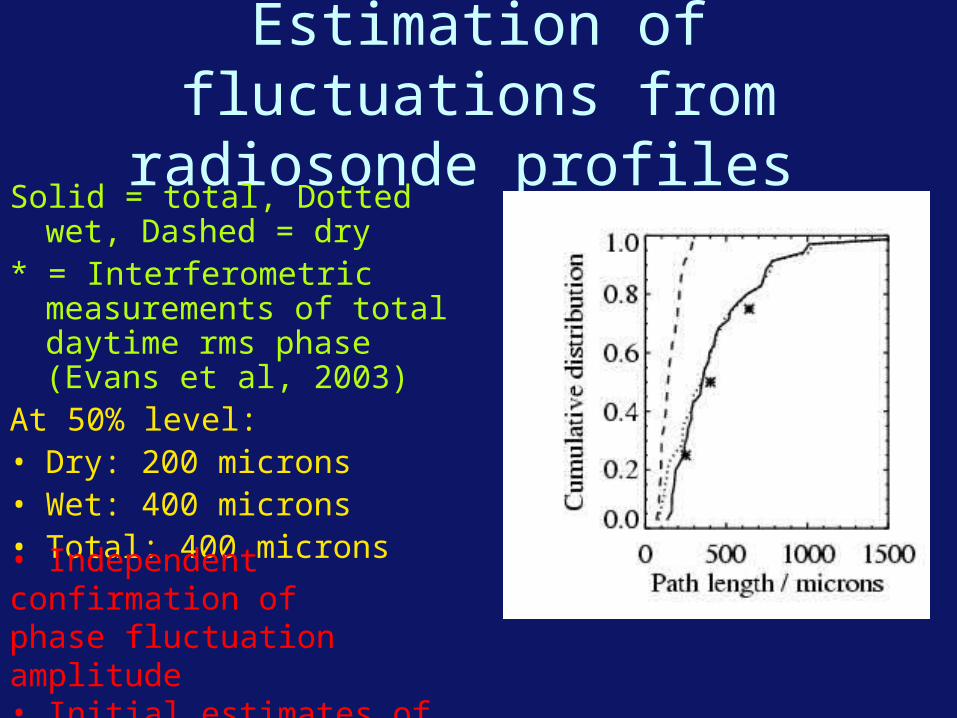
Estimation of fluctuations from radiosonde profiles

Solid = total, Dotted wet, Dashed = dry

* = Interferometric measurements of total daytime rms phase (Evans et al, 2003)

At 50% level:• Dry: 200 microns• Wet: 400 microns• Total: 400 microns

• Independent confirmation of phase fluctuation amplitude• Initial estimates of dry fluctuation component

Daytime structure function

• Solid = dry • Dot dashed = wet• Dotted = cross-

correlation term• Consistent with

Kolmogorov spectrum on small scales

Nocturnal mean profiles

Gradient of temperature profile opposite sign fromwater vapour profile

Evolution of night time fluctuations

Hei

gh

t / k

m

0

0.6

-0.3 0.3Horizontal distance / km

QuickTime™ and aDV/DVCPRO - NTSC decompressor

are needed to see this picture.

Location of dry, wet and total refractive index fluctuations

Negative correlation between wet and dry fluctuations near ground

Nocturnal structure function• Blue dashed = wet;

black solid = dry• r.m.s. wet

fluctuations ~ 2 x r.m.s dry

• Exponent of wet: 1.0, dry: 0.8

• Turn over around 800m (~ depth of layer)

Simulations of phase correction

• AIPS++ code written by Mark Holdaway• Combines Mark’s fast switching simulator with our 3-D

simulations of atmosphere• WVR simulated using `am’ radiative transfer code to

calculate brightness temperatures (Scott Paine)

Correction process: WVR

WVR: rms error

Conclusions

• Now have realisations of the atmosphere at Chajnantor for day and night conditions

• Dry and wet fluctuations have different distributions depending on time of day

• Have developed simulations of FS+WVR phase correction

• Future plans: – Investigate different phase correction strategies– Validation of the two ALMA prototype WVRs on

SMA