atmospheric turbulence and astronomical adaptive optics€¦ · atmospheric turbulence monitors •...
TRANSCRIPT

Atmospheric Turbulence and Astronomical Adaptive Optics
Matthew Britton
Caltech Optical Observatories

Outline• Atmospheric turbulence profiles
• Turbulence and image quality
• Angular anisoplanatism
• PSF estimation and deconvolution
• Differential tilt jitter
• The PSF of a laser guide star AO system
• Wide field adaptive optics architectures

Atmospheric Turbulence

Atmospheric Turbulence
WavefrontPhase
1.25 µm PSF
1.65 µm PSF
2.2 µm PSF

Atmospheric Turbulence Monitors
• Differential Motion Measurement (DIMM)
• Slope Detection and Ranging (SLODAR)
• Sonic Detection and Ranging (SODAR)
• Scintillation Detection and Ranging (SCIDAR)
• Shadow Band Ranging (SHABAR)

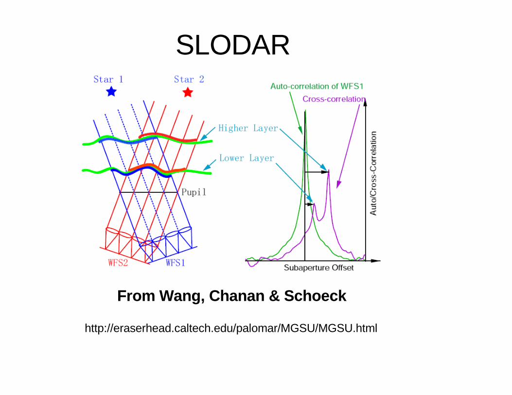
SLODAR
From Wang, Chanan & Schoeck
http://eraserhead.caltech.edu/palomar/MGSU/MGSU.html

Scintillation
5 meters
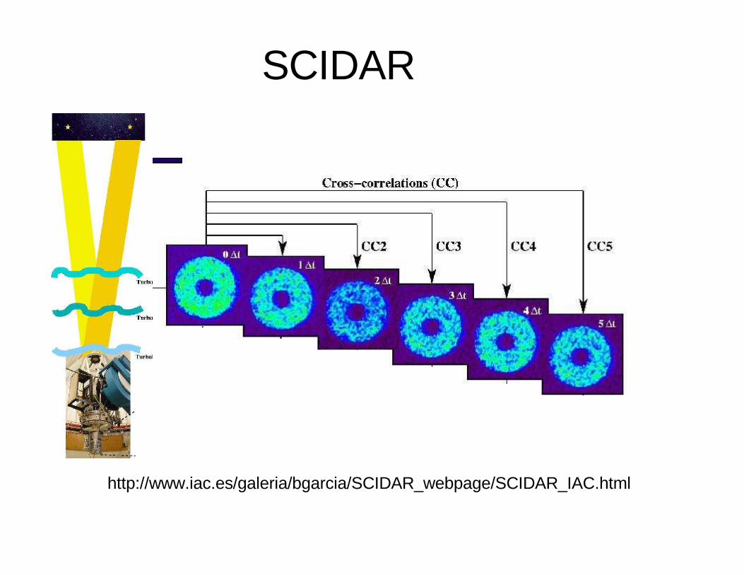
SCIDAR
http://www.iac.es/galeria/bgarcia/SCIDAR_webpage/SCIDAR_IAC.html

Multi Aperture Scintillation Spectrometry
http://www.ctio.noao.edu/~atokovin/profiler/index.html

DIMM/MASS
http://odata1.palomar.caltech.edu/massdimm/

Fried Parameter and Seeing
5/3
0
2200 )(423.0
−∞
= ∫ zCdzkr n
The Fried parameter r0 is the lateral coherence scale of the wavefront phase
0/ rSeeing λ=

Fried Parameter Variability
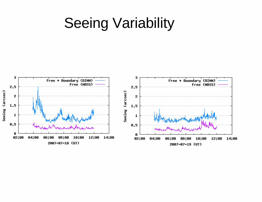
Seeing Variability

Seeing and r0 Statistics

Atmospheric Turbulence and Image Quality

The Long Exposure Point Spread Function
Diffraction limit(λ/D)
Seeing limit(λ/r0)
Seeing limit (x40)

Long Exposure Seeing Limited PSF Variability
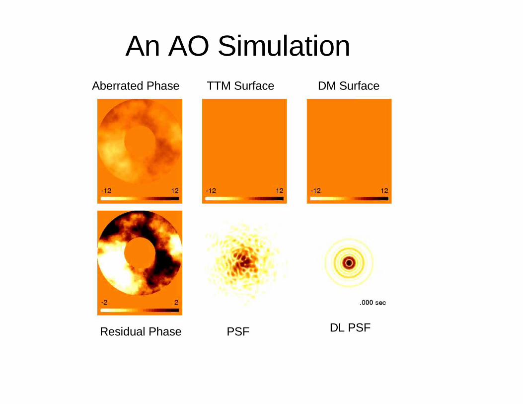
An AO SimulationAberrated Phase TTM Surface DM Surface
Residual Phase PSF DL PSF

Strehl Ratio vs Time

Guide Star Strehl Variability
3/5
0
= 2
r
dFF ασ
• Short term Strehl variability arises from the random realizations of atmospheric turbulence.
• Long term Strehl variability arises from the evolution of the atmospheric turbulence profile and the resulting change in AO system performance. For example, fitting error for an AO system with subapertures of size d is

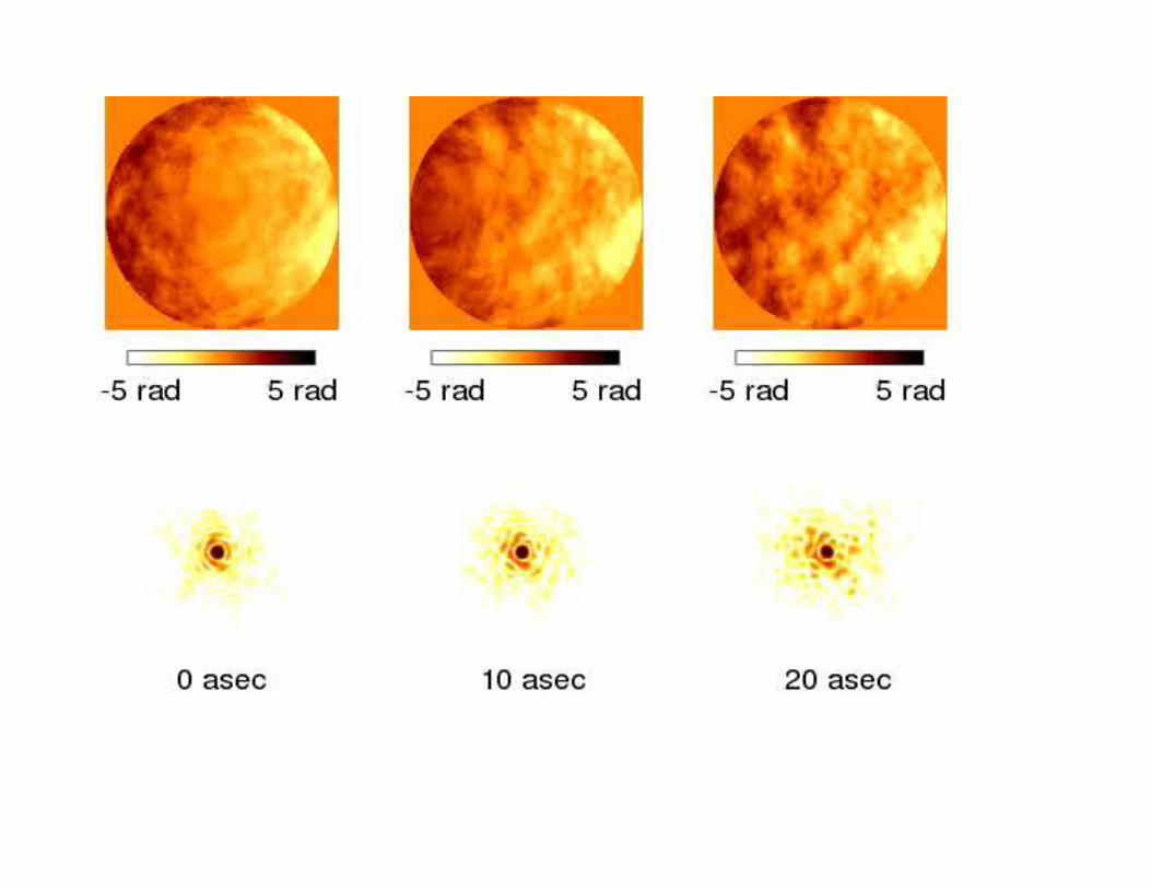
Angular Anisoplanatism
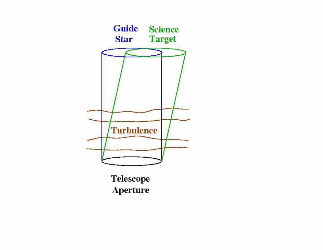

30”
Anisoplanatic Wavefront Phase Errors

30 asec separation
http://www.gemini.edu/sciops/instruments/adaptiveOptics/MCAO.html

Isoplanatic Angle
[ ] 5/32091.2
−
5/30 = µθ k
∫ = 3/523/5 )( zzdzCnµ
Θ0 is the angular decorrelation scale for wavefront phase aberrations arising from atmospheric turbulence.
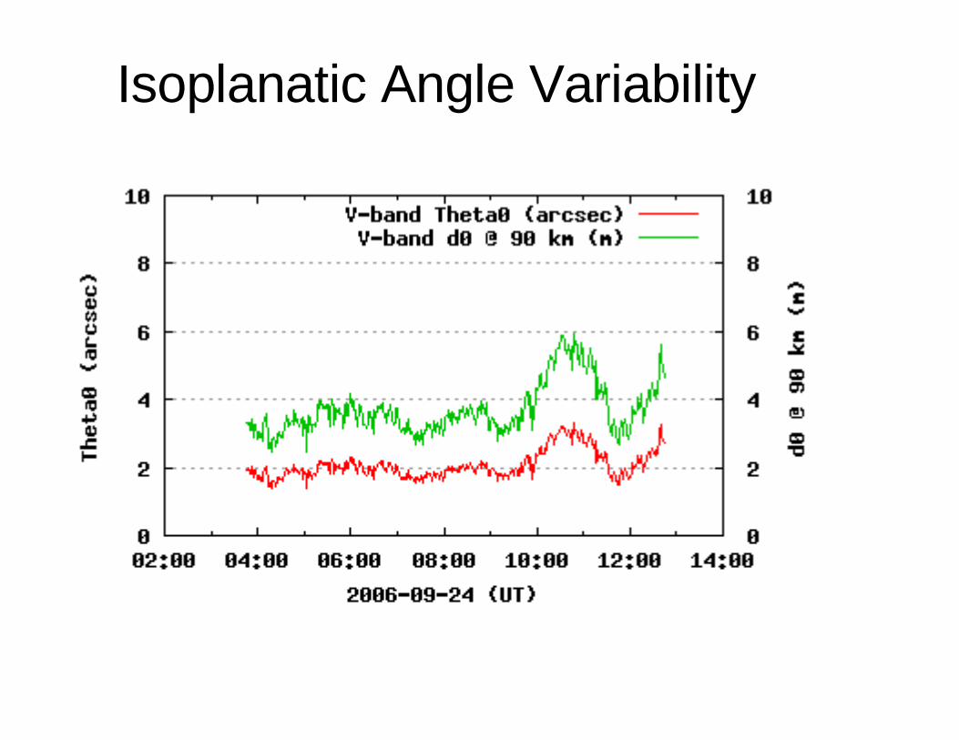
Isoplanatic Angle Variability

Θ0 Statistics
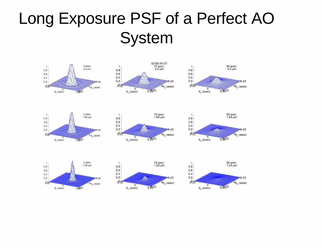
Long Exposure PSF of a Perfect AO System

Trapezium Images from Palomar
Guide star
Stars 1,2

Astronomical Impact of PSF Variability in Time and Field
• Turbulence profile variability is not stationary on observational timescales, so PSF variability doesn’t average away.
• Variations depend on turbulence and wind profiles, which impact AO system performance and anisoplanatic degradation.
• Variability in Strehl ratio can be factors of several on timescales of a minute or less.
Quantitative Applications of Astronomical Adaptive Optics
• Differential photometry
• Differential astrometry
• High contrast imaging
• Imaging and IFU spectroscopy of resolved objects
To understand the level of precision AO can provide, one must understand the consequences of turbulence profile variability on PSF stability in a particular observational context.
PSF Estimation and Deconvolution

PSF Estimation
• From a PSF calibration star
• From the data
• From a parameterized model
• From a measured turbulence profile

The Anisoplanatic Transfer Function
[ ] )()(5.0exp)( rOTFrDrOTF gsaploa
��� −=
{ }3/53/53/53/5
0
220
3/8 22)(2)( abababnapl zrzrrzzCdzkrD θθθ������� −−+−+Ξ= ∫
∞

PSF Estimation from Cn2 Profile
Guide Star Companion
[ ] )()(5.0exp)( rOTFrDrOTF oaaplgs
��� =−

Observed and Predicted PSFs
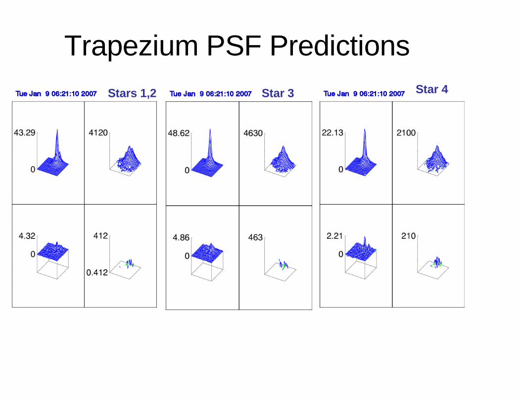
Trapezium PSF PredictionsStars 1,2 Star 3 Star 4

Deconvolution

Observations of a Quadruple

Modelling the Observation

Differential Tilt Jitter

Differential Tilt Jitter
≈
2
||
⊥
1
367.2
2
2
2
3/1 DD
θµσσ
To leading order


Tilt Jitter vs Angular Separation

Probability of the Measurements
{ }))(5.0exp)( rrrrrP T −(Σ−−∝ −1
( )( )jjiiij rrrr���� −−=Σ

Grid Astrometry
∑=i i
i
r
rs 2�
��
r7
r3
r5
r1
AATs Σ=Σ�

Grid Astrometry in Trapezium
N
1
N
1
N
1 t
1300 uas in 30 sec
Cameron, Britton & Kulkarni, in prep.
25 Images Averaged 10 stars averaged
Focal Anisoplanatism

LGS Adaptive Optics

Focal Anisoplanatism Parameter
−
Η.5=
−
25/35/3
5/3
2
200 452.
Hkd
µµ
In the differential wavefront phase between the LGS and the science target, d0 is the size of the coherence patch in the pupil plane.

d0 Variability

d0 Statistics
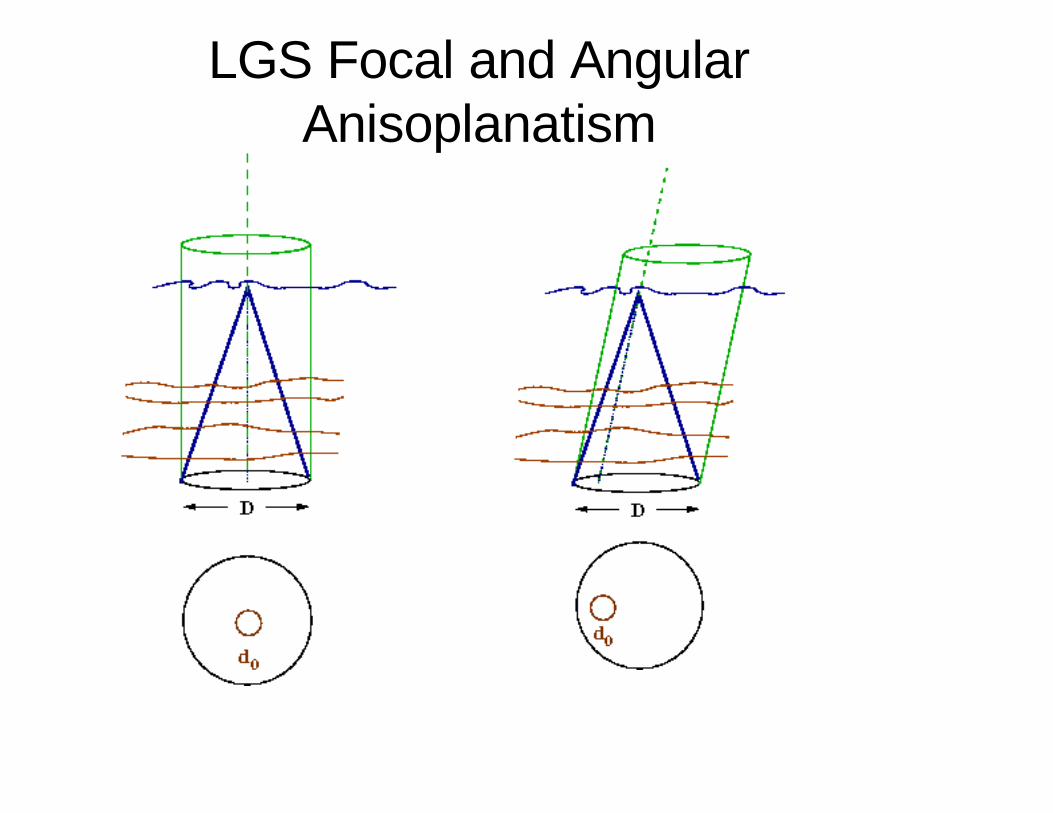
LGS Focal and Angular Anisoplanatism

Strehl Histories

The LGS PSF
==
H
km
m
D
H
Dc
90
30"702θ
The PSF is stable over a field of view of size
The PSF core width is
1
==00
450
d
m
mmas
dw
µλλ

Wavefront Sensing with Multiple Laser Beacons

Multiconjugate Adaptive Optics

ESO Multiconjugate AO Demonstrator
• Uses two 60 actuator bimorph deformable mirrors conjugated to 0km, 8.5km• Wavefront sensing performed with three natural guide stars

Multiobject Adaptive Optics
Optically separate the light from each science target and correct wavefront phase aberrations using a deformable mirror
Summary
• Measurement of atmospheric turbulence profiles• Effects of turbulence on image quality• Variability of the AO PSF in time and field • Estimation of the AO PSF• Quantitative applications of AO• The motivation for future wide field astronomical adaptive
optics architectures
Thank you