> TGRS-2008-00629.R1<

1

Abstract— New algorithms for total atmospheric water vapor

content (Q) and total cloud liquid water content (W) retrieval from satellite microwave radiometer data, based on Neural Networks (NNs) and applicable for high latitude open water areas, were developed. For algorithm development, a radiative transfer equation numerical integration was carried out for Special Sensor Microwave/Imager (SSM/I) and Advanced Microwave Scanning Radiometer (AMSR-E) channel characteristics for non-precipitating conditions over the open ocean. Sets of sea surface temperatures less than 15°C, surface winds and radiosonde reports collected by Russian research vessels served as input data for integration. It was shown that NNs perform better than the conventional regression techniques. Q retrieval algorithms were validated both for SSM/I and AMSR-E instrument using satellite radiometric measurements collocated in space and time with polar station radiosonde data. The resulting SSM/I and AMSR-E retrieval errors proved to be 1.09 kg/m2 and 0.90 kg/m2 correspondingly. For SSM/I Q retrievals the algorithms were compared with Wentz global operational algorithm. This comparison demonstrated the advantages of NNs-based polar regional algorithm in comparison with Wentz global one. The retrieval errors proved to be 1.34 kg/m2 and 1.90 kg/m2 (~40% worse) for NNs and Wentz algorithms correspondingly.

Index Terms— Microwave radiometry, Algorithms, Water, Neural networks

I. INTRODUCTION ECENT synthesis reviews based on the available observational data provide a coherent portrait of the

Manuscript received October 6, 2008. This work was supported by Japan

Aerospace Exploration Agency (project AD2-3rdRA-ENTRY AMSR013 and GCOM 1st RA project 111), Research Council of Norway (project 179125/S30) and by a Russian Fund of Basic Research, Far Eastern Branch (RFBR FEB grant 06-05-96076).

L. P. Bobylev is with Scientific Foundation "Nansen International Environmental and Remote Sensing Centre" (NIERSC), 199034 St. Petersburg, Russia (e-mail: leonid.bobylev@niersc.spb.ru).

E. V. Zabolotskikh, is with NIERSC, 199034 St. Petersburg, Russia (phone: 7-812-324-5103; fax: 7-812-324-5102; e-mail: elizaveta.zabolotskikh @niersc.spb.ru).

L. M. Mitnik is with V.I. Il’ichev Pacific Oceanological Institute, Far Eastern Branch Russian Academy of Science (POI FEB RAS), 690041 Vladivostok, Russia (e-mail: mitnik@poi.dvo.ru).

Maia L. Mitnik is with POI FEB RAS, 690041 Vladivostok, Russia (e-mail: maia@poi.dvo.ru).

Arctic climate change, indicating that the last 2 - 3 decades have experienced unusual warming over the northern Eurasia and North America [1], reduced Arctic sea ice [2], glaciers and snow cover [3], marked changes in the Arctic Ocean hydrography, increased river runoff into the Arctic, increased tree growth in the northern Eurasia, reduced tundra areas, and thawing permafrost [4]. These changes are consistent with the observed global warming associated with the increasing concentration of greenhouse gases (GHGs) in the atmosphere [5]. A consensus from coupled atmosphere-ocean model simulations of increasing GHGs scenarios is that the anthropogenic global warming will continue and be enhanced in the northern high latitudes [6], [7] due to complex feedback mechanisms in the atmosphere – ocean - ice system. This supposes that the Arctic may be the region where the most rapid and dramatic climate changes might take place during the 21st century. However, both instrumental observations and modeling show that the Arctic is the region of large natural climate variability [8], [9] complicated by fluctuating atmospheric conditions and influenced by the Arctic Oscillation [2], [10]. In depth analyses of the Arctic climate signal-to-noise ratio is therefore a prerequisite for proper quantification of the human-induced contribution to existing and future changes in the Arctic climate system. Therefore, additional observational studies are needed including changes of the Arctic atmosphere parameters such as water vapor and cloud liquid water content.

Water vapor is one of the major greenhouse gases and the most important gaseous absorber of the infrared radiation in the atmosphere. Therefore it is exceptionally important to know how the water vapor content and distribution in the atmosphere will be affected by the anthropogenic increase in other greenhouse gases, particularly in carbon dioxide. The existing estimates show that in the warmer world the concentration of water vapor in the atmosphere should increase [11]. This follows from the assumption that the relative humidity is constant when the atmosphere gets warmer. Therefore, the warming of the atmosphere caused by carbon dioxide concentration growth should lead to the increase in the saturation water vapor pressure and consequently increase in water vapor concentration. This, in its turn, will enhance further the greenhouse effect. Climate

Atmospheric Water Vapor and Cloud Liquid Water Retrieval over the Arctic Ocean Using

Satellite Passive Microwave Sensing Leonid P. Bobylev, Associate Member, IEEE, Elizaveta V. Zabolotskikh, Leonid M. Mitnik,

and Maia L. Mitnik

R

> TGRS-2008-00629.R1<

2

models indicate that this important positive feedback increases the sensitivity of surface temperatures to carbon dioxide by nearly a factor of two [12]. However, there is no consensus on this conclusion. The atmospheric storage of water vapor is not yet well studied [13], and many investigations are being conducted presently to estimate water budget and recycling ratio (the fraction of precipitation over a region that originated as evaporation from the same region) [14], [15].

Cloud liquid water influences the radiation coming to the Earth’s surface and thereby strongly affects the surface energy flux. Generally the role of clouds in the climate system is poorly known. Therefore, the long-term high-quality well-maintained observations of atmospheric water vapor and cloud liquid water content are necessary [16] including observations over the Arctic. They are essential both for the study of the variability and trends of these parameters and detachment of anthropogenic effects from natural climate variations.

Such long-term observations of the water content in the Arctic atmosphere can be provided by the satellite microwave radiometers over the open water [17] – [20]. Both atmospheric water vapor content (Q) and cloud liquid water content (W) over the oceans have been successfully retrieved from satellite microwave sensors, such as Scanning Multichannel Microwave Radiometer (SMMR) on board the Nimbus 7 and Special Sensor Microwave/Imager (SSM/I) on board the DMSP series satellites. Comparatively recently these opportunities have been widened and enriched by the launch of Advanced Microwave Sounding Radiometer (AMSR-E) on board the Aqua satellite. The latter gives new possibilities, associated with additional lower frequency channels at 6 and 10 GHz, and improved spatial resolution.

However, despite a comparatively long history of satellite passive microwave observations and their advantages, the retrievals of geophysical products from microwave radiometer data have always had large errors under significantly changing environmental conditions [21]. Also, Q and W retrievals from SSM/I and AMSR-E data have always been limited to the ice-free ocean regions. Many algorithms have been developed during the period of satellite passive microwave observations for Q and W retrievals including Neural Networks based ones [20], [22] - [24]. But so far none of the SSM/I or AMSR-E algorithms were developed specifically for the Arctic conditions. Great potential in obtaining water vapor fields over the Arctic belongs to such microwave sounders as Advanced Microwave Sounding Unit (AMSU) [25]. The methods exploring AMSU data allow water vapor retrievals over the ice but unfortunately so far they can be successfully applied only in dry (Q < 7 kg/m2) atmospheres. In [25] a new technique is suggested making possible Q retrievals over ice from AMSU data up to 15 kg/m2, but the retrieval errors are about 3 kg/m2, and the algorithm requires information about sea ice emissivities that restricts its application. Therefore, prior to processing satellite passive microwave data with the goal of developing a water vapor climatology for the Arctic, there is a strong need in having precise polar retrieval

algorithms tuned for the specific Arctic environmental conditions. Such algorithms should be developed separately for the open water and ice-covered areas.

This study is devoted to the development of specific high latitude algorithms mainly for the atmospheric water vapor content Q, but also for cloud liquid water content W retrievals from satellite radiometer measurements over the open ocean having in mind the follow-up studies, including both expansion of the area (Marginal Ice Zone and possibly ice-covered areas) for the algorithm application and estimation of the Arctic atmospheric water vapour variability and trends with relation to the Arctic climate change. The algorithms are physically-based, based on the Radiative Transfer Equation (RTE) solution for the atmosphere-ocean system using Neural Networks (NNs) as an inversion operator.

Computer simulations of the brightness temperatures (TB) were carried out for the input data sets consisting of radiosonde reports and values of ocean surface parameters such as sea surface temperature (Ts), salinity and wind speed (V). These simulations were done for frequencies, polarization, sensitivity, and sensing geometry of SSM/I and AMSR-E instruments, described in Section II.

For the development of the specific regional Arctic algorithms the appropriate input data set of the oceanic and atmospheric parameters for the latitudes north to 45°N with Ts < 15°C was created from Russian research vessel measurement data. Data collection for such an extended region was dictated by the task of measuring water vapor fluxes out of the Arctic into the middle latitude areas and vice versa over times. Initially, considering that the Ts influences strongly upon the sea surface emissivity and such a dependence is much non-linear, the selected data were subdivided into two subsets – specifically for polar waters with Ts ≤ 5°C, and for the middle latitude water with 5°C < Ts < 15°C, which were further used for training separate inversion algorithms. But it was found that Neural Networks handled effectively sea surface emissivity non-linearity: the algorithms trained separately for different Ts ranges performed not better than one general algorithm trained on the data set for the whole Ts range: Ts < 15°C. The data used for algorithm development are described in Section III. Data set of collocated in space and time satellite radiometer and radiosonde data from polar island stations used for validation/comparison purposes is described in Section VI.

The radiative transfer model of the atmosphere-ocean system, used in the study, implied the absence of scattering, i.e. non-precipitating clouds, and the absence of sea ice. The accuracy of the brightness temperature TB

p(ν) calculations for the frequency ν and polarization p depends on the uncertainties in the coefficients of electromagnetic radiation-medium interaction. Description of the microwave radiative transfer model and its restrictions is given in Section IV.

The main task of this study, as it was mentioned earlier, is the development of the algorithm for Q retrieval. However, simultaneously the total cloud liquid water content W retrieval algorithm is also suggested both as a distinct method and as an

> TGRS-2008-00629.R1<

3

additional facility for Q-algorithm tuning and validation. Neural Networks technique was chosen as a method for TB inversion into Q and W, and Linear (L), Non-Linear Quadratic (NL) and Logarithmic (LG) functions were used as alternative inversion techniques for the theoretical comparison purposes. Section V describes in detail Q and W retrieval algorithms, their accuracy and sensitivity to the systematical bias in the radiometer channels.

Theoretically developed algorithms were applied to SSM/I and AMSR-E measurement data. Validation of Q retrieval algorithms was carried out by means of the comparison with radiosonde data from small polar island stations. Indirect validation of W retrieval algorithm was done by means of the comparison of the cloud liquid water fields, obtained from passive microwave measurements, with infrared and visible images. At last, the comparison of Q values retrieved with NNs and Wentz Benchmark Pathfinder decode4a algorithm was done for the same polar island station data. The procedure of validation and the results obtained are described in details in Section VI. Comparison of the algorithms is described in Section VII. The summary of the major results and the conclusions are presented in Section VIII.

II. INSTRUMENT DESCRIPTION

A. Special Sensor Microwave/Imager The Special Sensor Microwave/Imager (SSM/I) is installed

onboard the Defense Meteorological Satellite Program (DMSP) spacecrafts placed in a circular sun-synchronous near-polar orbit at the altitude of approximately 833 km [26]. The active portion of the scan covers a swath of 1 400 km with the incidence angle at the Earth surface of approximately 53º. The sensor consists of 7 separate total-power radiometers sharing a common feedhorn. These 7 radiometers take dual-polarization measurements at 19.35, 37.0, and 85.5 GHz, and only vertical-polarization measurements at 22.235 GHz. The channel footprint varies with the channel frequency, the position in the scan, along the scan or along the track direction and the altitude of the satellite. The 85 GHz footprint is the smallest with a size of 13 x 15 km and the 19 GHz footprint is the largest with a size of 43 x 69 km. The sensitivity varies not exceeding 0.5 K for all the channels except 85 GHz. All brightness temperatures at the lower frequencies are resampled to a common location and resolution of 25 km (the channels at 85 GHz to 12.5 km). This resampling reduces the effective noise to the order of 0.2 K. The data from the DMSP satellites are received and used at operational centers continuously. The first in the series of SSM/I was launched in June 1987, and currently there are three satellites in orbit.

B. Advanced Microwave Scanning Radiometer The Advanced Microwave Scanning Radiometer (AMSR)

launched onboard the Aqua and ADEOS-II (now not functioning) satellites in 2002 (on the Aqua it is abbreviated as AMSR-Earth Observation System or AMSR-E) is similar

to SSM/I. AMSR-E takes dual-polarization observations at the 6 frequencies: 6.925, 10.65, 18.7, 23.8, 36.5, and 89.0 GHz. From the altitude of 705 km it measures the upwelling Earth brightness temperatures with a resulting swath width of 1 445 km. The nadir angle is fixed at 47.4º which results in an Earth incidence angle of 55.0º ± 0.3º. During a scan period the sub-satellite point travels 10 km. The instantaneous field-of-view for each channel is different; however, Earth observations are recorded at equal sample intervals of 10 km (5 km for 89 GHz channels) along the scan. The sensitivity (noise equivalent temperature) for the channels from 10.65 up to 36.5 GHz is about 0.6 K [27] and about 1.1 K at 89 GHz.

It should be noted that the instrument calibration for AMSR-E is more complicated than for SSM/I, for which it can be considered as well-established.

III. DATA Two arrays of data were used in the study. The first array

consists of the data used for the algorithm development. These data include the set of in-situ measurements of oceanic and atmospheric parameters and the corresponding set of simulated values of the brightness temperatures.

For the brightness temperature calculations the data set of the oceanic and atmospheric parameters was composed from radiosonde (r/s), meteorological - wind speed, forms and amount of clouds (percentage of cloud cover) - and hydrophysical (Ts and salinity) simultaneous measurements. These measurements were taken by research vessels of the Far Eastern Research Hydrometeorological Institute (USSR/Russia) during the period of 1966 - 1993. Only part of this data set, with Ts values less than 15ºC, was selected for the polar algorithm development. This selection was based on the climate atlas analysis, according to which the geographical region with latitudes higher than 45ºN is characterized by Ts < 15ºC. The selected data composed the Arctic input data set. It consists of 789 radiosondes with simultaneous Ts and salinity measurements.

R/s profiles of air temperature, humidity and pressure were complimented by the cloud liquid water content (w) profiles. These profiles were constructed by summarizing w measurements for different forms of clouds [28]. Forms and amount of clouds were determined by experienced meteorologists during radiosonde launching. The upper and lower boundaries of cloudiness were estimated using relative humidity profiles. Uniform w profiles were taken for the clouds with thickness less than 1 km with typical w values of 0.05 - 0.10 g/m3. For clouds with thickness greater than 1 km the w profiles were described by triangle function. In this case the cloud liquid water content maximum was located at the one third of thickness below the upper boundary of cloudiness. This maximum increases with the increase of the cloud thickness. A linear relation was assumed between w and the cloud amount. The decrease of w values with the decrease of cloud temperature for the given form of clouds was also

> TGRS-2008-00629.R1<

4

taken into account, basing on the statistical data, describing liquid water content distribution in the clouds of varying forms and temperatures.

Finally the data set was artificially increased by including surface wind speed values randomly and uniformly distributed between 0 and 16 m/s. Thus the resulting data set includes 14 202 members. Since the sea surface emissivity depends on Ts and such dependence is a non-linear one, firstly this data set was divided into two subsets: for polar waters with Ts ≤ 5°C, and for the middle latitude water with 5°C < Ts < 15°C. The aim of such division was training different NNs inversion algorithms for these two Ts ranges. Later it was found that the algorithms trained separately for two Ts ranges had no advantages in comparison with a single algorithm trained using the whole data set with Ts < 15°C. This confirms the ability of Neural Networks to be adjusted effectively to various kinds of non-linearity. So, in the further work the general set of data Ts < 15°C was used. Additional restriction was applied to the values of polarization difference ∆T37 = TB

V(37 GHz) - TBH(37 GHz) at 37 GHz (SSM/I) or 36.5 GHz

(AMSR-E) in the observed brightness temperatures. Data with ∆T37 < 10 K were discarded (less than 1% of all data) as most probably associated with precipitation. Handling these data needs special consideration. Such low values of polarization difference are caused most likely by dense atmosphere due to precipitation with the intensity higher than 3 – 5 mm/h impending surface polarized signal. High winds under more transparent atmosphere can also decrease the ∆T37 (winds of 20 m/s lead to decrease of 12 – 18 K in polarization difference). Q and W retrievals are also possible under such conditions but a special algorithm should be developed.

Finally, after discarding, the resulting data set (DS1) consists of 14 110 simultaneous data. For the algorithm development this data set was randomly divided into two subsets - training and testing. The training subset was used for Neural Networks training, and the testing one - for the algorithm performance assessment. The statistical characteristics of the total atmospheric water vapor content for training and testing subsets are presented in Table I.

TABLE I

STATISTICAL CHARACTERISTICS OF THE TOTAL ATMOSPHERIC WATER VAPOR CONTENT Q FOR TRAINING AND TESTING SUBSETS OF DATA (N – THE SAMPLE

SIZE; Qmin, Qmax,, Qmean AND σQ – MINIMUM, MAXIMUM, MEAN VALUES AND STANDARD DEVIATION OF THE TOTAL ATMOSPHERIC WATER VAPOR

CONTENT) Data

subset N Qmin,

kg/m2 Qmax,

kg/m2 Qmean,

kg/m2 σQ,

kg/m2 training 7 058 0.6 33.4 8.3 5.7

testing 7 144 0.6 33.4 8.5 5.8

The second array of data (DS2) consists of the

measurements used for Q-retrieval algorithm validation. These data include SSM/I and AMSR-E measurements collocated in space and time with 12 hour radiosonde measurements from three polar island stations: Jan Mayen, Bjornaya and Torshavn. The data cover the whole 2005 year (each day) and encompasses the range of Q variability in the Arctic. SSM/I

calibrated brightness temperatures were taken from DMSP F15 radiometer from Global Hydrology Resource Center (GHRC). Also part of these data was taken for the comparison of NNs-based SSM/I algorithm with the Wentz SSM/I algorithm performance. AMSR-E calibrated brightness temperatures were provided by Japan Aerospace Exploration Agency. Ready made Wentz Q fields were taken also from GHRC. Data, used for the comparison, included only Torshavn radiosonde measurements since for the other two stations Wentz algorithm was not applicable due to spacious mask of possible ice. In more details the description of the validation/comparison data sets can be found in Section VI.

IV. RADIATIVE TRANSFER MODEL The governing factor of any retrieval algorithm is the

atmosphere-ocean system (AOS) geophysical model which relates geophysical parameters to observed brightness temperatures. Its uncertainties define the uncertainties in forward modeling. We restrict our model by non-precipitating conditions using absorption-emission approximation and neglecting microwave radiation scattering on large rain drops and ice particles. Such an approximation is valid for the frequencies less than 37 GHz for clear and cloudy atmosphere and for light rain up to ~ 2 mm/h. It is estimated [29] that only 3% of all SSM/I global ocean observations relate to the rainfalls with rate more than 2 mm/h. So, non-scattering model is applicable to about 97% of all ocean observations. For latitudes higher than 45°N this assessment is all the more justified.

For the non-scattering approximation the AOS brightness temperature TB

V,H(ν,θ) at frequency ν, incidence angle θ and polarization P (vertical-V or horizontal-H) is a function of surface temperature Ts, sea surface emissivity χV,H, and total atmospheric absorption τ [30].

Under non-precipitating conditions in the microwave range of frequencies below 100 GHz the atmospheric absorption is defined by three components: oxygen, water vapor and cloud liquid water. It should be noted that the water vapor emission model uncertainties and selection of the instrument channels to be used in the retrieval are the predominant error sources for satellite-derived Q values.

The dependence of oxygen and water vapor absorption coefficients on frequency, temperature, pressure and water vapor density was studied by many researchers [31] – [34]. Special studies were devoted to the inter-comparison of the models and influence of the model parameters on the resulting satellite-derived water vapor values [35]. In our geophysical model we used oxygen and water vapor absorption coefficients from [31] with an exception for the frequency range 20 – 24 GHz, where the formulas from [34] were deployed. Incorrectly modeled water vapor absorption coefficients can lead to the errors in its following retrievals, though for typical values of water vapor in Arctic marine atmosphere this issue has less value than generally.

> TGRS-2008-00629.R1<

5

A precise knowledge of the complex dielectric permittivity of water ε is essential for studying the transfer of the microwave radiation in the AOS because it enters into the radiative transfer equations by two ways: firstly it refers to the sea water and defines the sea surface emissivity and reflectivity, and, secondly, it refers to the fresh water of the cloud droplets. The choice of a model for ε dependence on frequency, temperature and salinity, influences the calculated brightness temperatures. A number of studies were carried out recently [36] – [39]. This resulted in new models, updated regarding commonly used [40]. The latter, as it was shown by various authors [21], [41] – [43], is getting increasingly inaccurate with frequency increase.

For our calculations we took the model of Meissner and Wentz [39], since it is extensively validated and valid for frequencies up to at least 90 GHz for the fresh water in the temperature range between -20°C and +40°C including supercooled water, and for sea water for temperatures between -2°C and +29°C. This model has large distinction from the other models in the ε behavior for temperatures below 0°C and performs well under low temperatures which is most important for our polar case. Additional reason for this choice was that the models from [38] and [39] provided close results for ε calculations even for high frequency of 85.5 GHz.

To calculate brightness temperatures we also needed a model for sea surface emissivity χV,H(ν,θ) which for the calm sea surface depends only on dielectric constant of marine water (Frenel’s equations), but for the wind influenced sea surface needs additional definition.

Formulating a consistent theoretical model for the wind speed dependency of sea surface emissivity is very difficult. But there exist empirical models based on near-surface measurements. Such coordinated observations were performed, for example, in [44] by Aziz et al. during the Fluxes, Air – Sea Interaction, and Remote Sensing (FAIRS) experiment. The results obtained during FAIRS showed a good agreement with previous models [21], [45] - [48] and a good linear fit between emissivity and surface wind speed in the range of 4 - 16 m/s at three incidence angles (45°, 53°, and 65°) at 10.8 and 36.5 GHz. Some uncertainty for using these results for forward modeling in polar regions relates to the sea surface temperature restricted to only single value of Ts = 17°C. Slightly different results from [44] were obtained by Meissner and Wentz [49]. Here the isotropic (direction independent) wind induced emissivity for vertical and horizontal polarizations was derived by averaging globally over a large number of wind directions.

In our geophysical model we used the combination of wind induced emissivity models. For horizontal polarization we adopted [48], since it is in the best agreement with all the models referenced here but provides the values of derivatives of emissivity with respect to wind speed ∂χ/∂V for the whole range of frequencies from 6 to 90 GHz. For vertical polarization, to define ∂χ/∂V, we used a combination of [38], [39], [44], and [48] models to come to the best agreement

between them. After all the models for the microwave radiation interaction

with the atmosphere-ocean system had been defined, the brightness temperatures for frequencies, polarization and angles of incidence of SSM/I and AMSR-E instruments were calculated. Normally distributed radiometric noise with 0.5 K equivalent temperature was added to the resulted TB values, which then were included into the data set DS1, described in Section III. The whole matched-up data set DS1 of geophysical parameters Q, W (calculated from the corresponding radiosonde reports), Ts and V and simulated values of TB for SSM/I and AMSR-E served as a base for the inverse problem solution – for the algorithm development.

V. RETRIEVAL ALGORITHMS Several algorithms for the total atmospheric water vapor

content and cloud liquid water content retrievals from satellite passive microwave data are available in the literature. Some of them are based on purely statistical technique [17], [18] using collocated in-situ and satellite measurements. The other ones are physically-based, resting on the radiative transfer simulations [19], [21], [50], [51]. The established advantage of physically-based algorithms is their well developed theoretical basis.

Neural Networks (NNs) - based algorithms can also be both statistically and physically-grounded. Their general point is that they don’t require a priori knowledge of the transfer function, which can be of any non-linear character. Such great method potential has been successfully used in a large variety of remote sensing applications, including our specific case of Q- and W-parameter retrievals [20], [22], [52] – [54].

The algorithms suggested in this study refer to physical, based on RTE simulations, NNs regional techniques for the total atmospheric water vapor and total cloud liquid water retrievals from SSM/I and AMSR-E radiometric data applicable for the Arctic and Sub-Arctic areas. Neural Networks here play a role of inverse function. For the theoretical comparison of NNs technique with other alternative inversion functions we used Linear (L), Non-Linear Quadratic (NL) and Logarithmic (LG) regressions. The choice of the logarithmic function was determined by the close to exponential dependency of brightness temperature, through total atmospheric absorption, on Q and W. This approach was first proposed in [55] and then successfully applied in different modifications by several researchers to retrieve Q and W from satellite microwave observations. All regression coefficients were derived from the same training data set (randomly selected half of DS1) on which NNs algorithms were trained, and applied to the same testing data set (the other half of DS1) to which NNs algorithms were applied.

Standard Neural Network of Multilayer Perceptron (MLP) type with feedforward backpropagation of errors was used to connect simulated brightness temperatures with parameters Q

> TGRS-2008-00629.R1<

6

and W. MLP Neural Network is a processing block in which input (in our case TB at the radiometer channels) and output (Q and W) parameters of the task are connected via the system of neurons at hidden layers, relatively to input and output layers [56]. The neurons are connected among themselves and with input and output parameters by weighted links (ω). The inputs of the Neural Network (TB) are processed using this block of weighted links (ω) and one or another weight activation function to produce an output (parameter P):

),( BTfP ω= (1)

Multiple output parameter schemes produce simultaneously

several output parameters whereas single output nets generate one parameter as a result. Neural Networks are trained using training data sets of input and output vectors. During training the weights of links are being varied in such a way that the root mean square difference F between known parameters (Pm) and processed input parameters (f(ω, TBm))

∑=

−=M

mBmm TfPF

1

2)),(( ω (2)

is turned to its minimum. Here m signifies the number of a

data set, M – the total number of data sets. There always exists a risk of overtraining NNs due to their

complexity. Overtraining results into the loss of NNs generalization features [57]. If NNs configuration is too simple, it may fail to conform to data, producing large F values. On the other hand, NNs should not be too complicated. In such a case the algorithm may perform well when applied to training data set, but results to large errors for another (testing) data set. In order to avoid such overtraining, each training procedure was conducted comprehensively, e.g. configuration had been sophisticated until the testing error began to increase. The training was carried out via supervised learning and feedforward backpropagation of errors, starting from various random initial weights to avoid getting local minima [58].

In the retrieval algorithms a single output parameter configuration was used, e.g. for water vapor and cloud liquid water separate Neural Networks were trained. The MLP configuration with a single hidden layer was used since in the tasks of the best approximation any continuous on a finite interval function can be approximated by a Neural Network of MLP type with one hidden layer [59]. The numerical experiments with other configurations confirmed that including additional layers led to rapid loss of the generalization capabilities, especially for noisy data.

At first different NNs were trained for three different ranges of Ts: Ts ≤ 5°C; 5°C < Ts < 15°C and the overall temperature range Ts < 15°C. But, as was found later, there was no difference in the performance of separately trained algorithms when they were applied to the testing data sets – either divided according to temperature range or not.

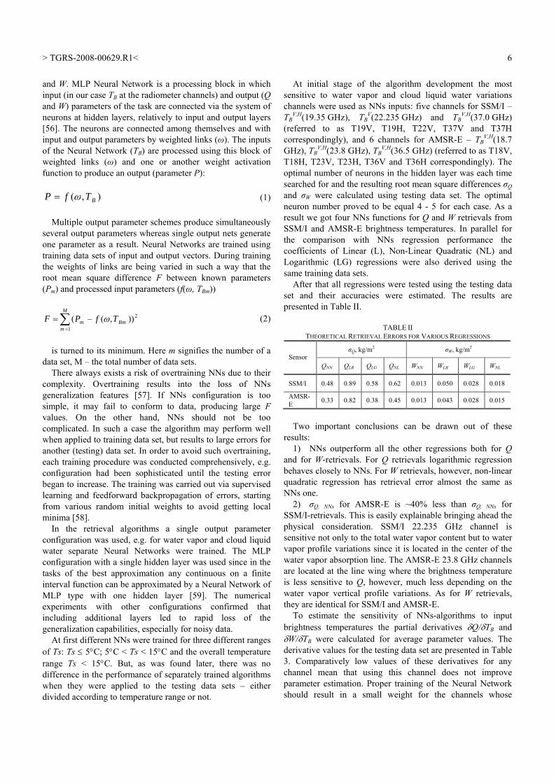
At initial stage of the algorithm development the most sensitive to water vapor and cloud liquid water variations channels were used as NNs inputs: five channels for SSM/I – TB

V,H(19.35 GHz), TBV(22.235 GHz) and TB

V,H(37.0 GHz) (referred to as T19V, T19H, T22V, T37V and T37H correspondingly), and 6 channels for AMSR-E – TB

V,H(18.7 GHz), TB

V,H(23.8 GHz), TBV,H(36.5 GHz) (referred to as T18V,

T18H, T23V, T23H, T36V and T36H correspondingly). The optimal number of neurons in the hidden layer was each time searched for and the resulting root mean square differences σQ and σW were calculated using testing data set. The optimal neuron number proved to be equal 4 - 5 for each case. As a result we got four NNs functions for Q and W retrievals from SSM/I and AMSR-E brightness temperatures. In parallel for the comparison with NNs regression performance the coefficients of Linear (L), Non-Linear Quadratic (NL) and Logarithmic (LG) regressions were also derived using the same training data sets.

After that all regressions were tested using the testing data set and their accuracies were estimated. The results are presented in Table II.

TABLE II

THEORETICAL RETRIEVAL ERRORS FOR VARIOUS REGRESSIONS

σQ, kg/m2 σW, kg/m2 Sensor

QNN QLR QLG QNL WNN WLR WLG WNL

SSM/I 0.48 0.89 0.58 0.62 0.013 0.050 0.028 0.018

AMSR-E 0.33 0.82 0.38 0.45 0.013 0.043 0.028 0.015

Two important conclusions can be drawn out of these

results: 1) NNs outperform all the other regressions both for Q

and for W-retrievals. For Q retrievals logarithmic regression behaves closely to NNs. For W retrievals, however, non-linear quadratic regression has retrieval error almost the same as NNs one.

2) σQ, NNs for AMSR-E is ~40% less than σQ, NNs for SSM/I-retrievals. This is easily explainable bringing ahead the physical consideration. SSM/I 22.235 GHz channel is sensitive not only to the total water vapor content but to water vapor profile variations since it is located in the center of the water vapor absorption line. The AMSR-E 23.8 GHz channels are located at the line wing where the brightness temperature is less sensitive to Q, however, much less depending on the water vapor vertical profile variations. As for W retrievals, they are identical for SSM/I and AMSR-E.

To estimate the sensitivity of NNs-algorithms to input brightness temperatures the partial derivatives δQ/δTB and δW/δTB were calculated for average parameter values. The derivative values for the testing data set are presented in Table 3. Comparatively low values of these derivatives for any channel mean that using this channel does not improve parameter estimation. Proper training of the Neural Network should result in a small weight for the channels whose

> TGRS-2008-00629.R1<

7

brightness temperatures are little or not sensitive to the parameter. Thus, the sensitivity estimation (see Table III) allowed us to exclude some channels from the input sets: T19V and T37V for SSM/I Q retrievals; T19V and T22V for SSM/I W retrievals; T18V and T36V for AMSR-E Q retrievals; and T18V and T23H for AMSR-E W retrievals. After such removals new algorithms were trained and tested the same way as initially, including derivation of the coefficients for all the other regressions considered. This procedure, as it was foreseen, did not result into increase of the errors.

TABLE III

SSM/I AND AMSR-E NNS INITIAL ALGORITHM SENSITIVITY TO INPUT TB FOR Q AND W RETRIEVALS

SSM/I

Channel 19H 19V 22V 37H 37V

δ<Q>/δTB (kg/m2)/K 0.10 0.09 0.61 -0.22 -0.01

δ<W>/δTB

(kg/m2)/K -0.011 -0.001 0.004 0.008 0.008

AMSR-E

Channel 18H 18V 23H 23V 36H 36V

δ<Q>/δTB (kg/m2)/K -0.22 -0.03 0.38 0.26 -0.20 0.00

δ<W>/δTB (kg/m2)/K -0.011 -0.002 0.000 0.003 0.009 0.008

At this the instrumental noise won’t so much influence the

results, since any systematical bias in TB (e.g. due to a problem of the radiative transfer model or calibration), which will be assimilated by the Neural Network and lead to biased results.

Thus, the final optimal NNs configurations for SSM/I and AMSR-E were fixed. These configurations are shown in Fig. 1.

T19H

T22V

T37H

Q

T19H

T37H

T37V

W

a

T18H

T23H

T36H

Q

b

T23V

T18H

T23V

T36V

W T36H

Fig. 1. Multilayer Perceptron Neural Network optimal configurations for Q and W retrievals over the areas north to 45ºN from SSM/I (a) and AMSR-E (b).

The new values of δQ/δTB and δW/δTB, derived under average Q and W, are presented in Table IV. These values are slightly changing with parameter change but not more than by 2-5%.

TABLE IV SSM/I AND AMSR-E NNS FINAL ALGORITHM SENSITIVITY TO INPUT TB FOR Q

AND W RETRIEVALS

Sensor SSM/I AMSR-E

Channel 19H 22V 37H 18H 23H 23V 36H

δ<Q>/δTB (kg/m2)/K 0.09 0.63 -0.20 -0.22 0.39 0.25 -0.20

Channel 19H 37V 37H 18H 23V 36V 36H

δ<W>/δTB (kg/m2)/K -0.005 0.003 0.015 -0.011 0.002 0.009 0.007

The estimation of the algorithm sensitivity to the bias in the

instrument channels was also carried out. It is an important stage of the study, associated with the existent uncertainties of the radiation transfer model and the calibration of microwave radiometers. Such estimation was done using the following procedure. A varying bias ∆TB from 0 up to 5 K was added by turns to separate channel brightness temperatures. As a result, the mean for the ensemble of retrieved parameters <Q> and <W> shifted to the other values – <Q’> and <W’>. The dependences of δ<Q> = <Q’> - <Q> and δ<W> = <W’> - <W> on ∆TB, which can be interpreted as the sensitivity of the algorithm to the calibration/geophysical model errors, for SSM/I and AMSR-E are shown in Fig. 2.

The knowledge of δQ/δTB and δW/δTB values in practice provides us with the tool for managing calibration/validation uncertainties. It is therefore quite important to know how these functions behave under various atmospheric absorptions. We showed that for Neural Networks - based algorithms they increase approximately linearly in absolute values up to τ ~ 0.2 - 0.3 and then remain nearly invariable.

For testing algorithm behavior for different parameter ranges, the root mean square errors σQ and σW were calculated for NNs-algorithms for SSM/I and AMSR-E as the functions of Q, W, and Ts values. The analysis of these functions, presented in Fig. 3, provides the knowledge about the algorithm performance under various environmental conditions and dependence of the retrieval results on the parameters Q, W and Ts. It can be concluded from the analysis of these dependencies that NNs-algorithms are more or less steady relatively to the sea surface temperature. Significant growth of the errors is observed when the cloud liquid water content increases. The errors also tend to rise gently with Q. The stable performance along with high retrieval accuracies characterizes NNs-algorithms as suitable for spatial and temporal water vapor variability studies. It can be resumed that the theoretical retrieval errors, calculated using simulated testing data set, are equal to σQ = 0.48 kg/m2, σW = 0.013 kg/m2 for SSM/I, and σQ = 0.34 kg/m2, σW = 0.013 kg/m2 for AMSR-E. The retrieval errors for the other regressions are 15 - 100% higher.

> TGRS-2008-00629.R1<

8

-0.04

-0.02

0.00

0.02

0.04

0.06

0.08

0 1 2 3 4 5

19H37H37V

-2

-1

0

1

2

3

4

0 1 2 3 4 5

19H22V37H

Sens

itivi

ty δ

<Q>

(kg/

m2 )

Sens

itivi

ty δ

<W>

(kg/

m2 ) a

b

-2

-1

0

1

2

3

4

0 1 2 3 4 5

18H23H23V36H

Bias ∆TB (K)

Sens

itivi

ty δ

<Q>

(kg/

m2 )

-0.06

-0.04

-0.02

0.00

0.02

0.04

0.06

0.08

0 1 2 3 4 5

18H23V36H36V

Sens

itivi

ty δ

<W>

(kg/

m2 )

Bias ∆TB (K)

Fig. 2. SSM/I (a) and AMSR-E (b) NNs algorithm sensitivity to systematical bias in the input channels for Q and W retrievals.

0.0

0.2

0.4

0.6

0.8

1.0

0 5 10 15 20 25 300.00

0.01

0.02

0.03

0.04

0 5 10 15 20 25 30

0.0

0.5

1.0

1.5

2.0

0.0 0.5 1.0 1.5 2.00.00

0.02

0.04

0.06

0.08

0.10

0.0 0.5 1.0 1.5 2.0

0.0

0.2

0.4

0.6

0.8

1.0

0 2 4 6 8 10 120.00

0.01

0.02

0.03

0.04

0.05

0 2 4 6 8 10 12

Atmospheric water vapor content Q (kg/m2)

Total cloud liquid water content W (kg/m2)

Sea surface temperature Ts (°C)

Atm

osph

eric

wat

er v

apor

con

tent

retri

eval

err

or σ

Q (k

g/m

2 )

Tota

l clo

ud li

quid

wat

er c

onte

nt re

triev

al e

rror

σW

(kg/

m2 )

Atmospheric water vapor content Q (kg/m2)

Total cloud liquid water content W (kg/m2)

Sea surface temperature Ts (°C)

Fig. 3. Resulting SSM/I (solid line) and AMSR-E (dash line) retrieval errors σQ and σW as functions of Q, W and Ts parameters.

VI. ALGORITHM VALIDATION Theoretically developed algorithms were validated for

SSM/I and AMSR-E total water vapor content retrievals against radiosonde data from three polar island stations - Jan Mayen (70.9ºN, 8.7ºW), Bjornoya (74.5ºN, 19.0ºE) and

> TGRS-2008-00629.R1<

9

Torshavn (62.0ºN, 6.8ºW). The radiosonde data for the whole year 2005 were used to ensure the representation of the water vapor for the whole range of its natural variability for all seasons. Radiosonde data are available for each day two times: at 00:00 UTC and at 12:00 UTC. However for SSM/I and AMSR-E radiometers only daytime (from 9:00 UTC to 14:00 UTC) paths were used which passed over the Norwegian Sea where the stations were situated. So, 12 hour radiosonde data collocated in time within 1.5 hour time difference with radiometric measurements were used for validation. The spatial collocation of pixels was done within the distance of 50 km from a station, but in such way that neither land, no coastal zone, able to influence the signal and lead to its misinterpretation, fell into the pixel used for validation. Measurements of 5 pixels within the distance of 50 km from a station were converted into water vapor content values (QSSM/I from SSM/I or QAMSR-E from AMSR-E measurements), averaged and compared with radiosonde water vapor content value Qr/s. Radiosonde data were downloaded from the University of Wyoming web site (http:// weather.uwyo.edu/upperair/sounding.html). Fig. 4 presents the distribution of Qr/s during the whole year 2005 based on the data of these 3 stations. Fig. 4 shows that the maximum water vapor values in the considered area don’t exceed 25-30 kg/m2, and the most values fall into the interval from 4 to 14 kg/m2. This means that the suggested algorithms were validated for this range of values, typical for the Arctic region.

Total water vapor content Q (kg/m2)

0.00

0.05

0.10

0.15

0 5 10 15 20 25 30

Fig. 4. Distribution of atmospheric total water vapor Qr/s over stations Jan Mayen, Bjornoya and Torshavn in 2005.

Careful selection of the collocated data was carried out before the validation. The water vapor and liquid water fields were built for every day to analyze these fields in the vicinity of the stations. This was done aiming at the exclusion from the comparison the situations with abrupt atmospheric changes or severe weather conditions such as passing atmospheric fronts, taking place right over the radiosonde stations. Such data, especially with large collocation time difference, were discarded from the validation data set DS2.

For the illustration Fig. 5 shows total water vapor field derived with NNs algorithm from SSM/I radiometer measurements on 3 June 2005 at 10:30 UTC. The sharp increase of water vapor in the vicinity of Torshavn Island is

associated with the abrupt atmospheric front. Obviously such data should be excluded from testing. Besides, the larger the collocation time difference is the more distant fronts need to be taken into account in dependence on the sea surface wind speed and direction.

Total water vapor content QSSM/I (kg/m2)

Fig. 5. Total water vapor content field over the Norwegian Sea area retrieved with NNs-algorithm from SSM/I measurements acquired on 3 June 2005 at 10:30UTC.

The total number of data collocations used for SSM/I

algorithm validation for the whole year 2005 amounted to 884. 31 data of 365 were discarded from Jan Mayen data due to either the absence of appropriate space and time collocation or due to the cases of atmospheric fronts (17 data). 84 data of 365 were discarded from Bjornaya data due to a) absence of collocation, b) ice in the vicinity of the station in February and March, and c) atmospheric fronts (25 data). 96 data of 365 were discarded from Torshavn data – mostly due to the absence of space collocation. Torshavn is situated far from the North Pole, so that many SSM/I and AMSR-E paths suitable for time collocation lie far away from Torshavn Island. 24 data of 96 refer to the cases of abrupt atmospheric fronts. The total number of data collocations used for AMSR-E algorithm validation amounted to 970 (more than for SSM/I due to larger number of space and time collocations).

radiosonde Qr/s (kg/m2)

NN

s ret

rieve

d Q

SSM

/I (k

g/m

2 )

y = 1.01xR2 = 0.96

0

5

10

15

20

25

30

0 5 10 15 20 25 30

Fig. 6. SSM/I NNs retrieved versus radiosonde total water vapor content over Jan Mayen, Bjornoya and Torshavn polar stations for the period of 2005.

The total Q retrieval error (root mean square difference)

calculated for the data set DS2 proved to be 1.09 kg/m2 for SSM/I and 0.90 kg/m2 for AMSR-E. For SSM/I separate

> TGRS-2008-00629.R1<

10

analysis for the stations was carried out: σQ totaled to 1.05, 0.85 and 1.34 kg/m2 for Jan Mayen, Bjornoya and Torshavn r/s data respectively. The corresponding scatter plot of retrieved from SSM/I QSSM/I versus radiosonde Qr/s is presented in Fig. 6. The correlation coefficient R2 is close to 1, which confirms high algorithm performance. The bias is about

-0.5 which means that the algorithm tends to underestimate radiosonde data. In Fig. 7 the dependence of the SSM/I retrieval error on the atmospheric water parameters is shown. It is seen that the absolute algorithm error slightly increases with Q and W increase.

0.0

0.5

1.0

1.5

2.0

2.5

3.0

0.0 0.1 0.2 0.3 0.4 0.5 0.60.0

0.5

1.0

1.5

2.0

2.5

0 5 10 15 20 25 30

a b

NNs retrieved QSSM/I (kg/m2)

SSM

/I ro

ot m

ean

squa

re N

Ns

retri

eval

err

or σ

Q (k

g/m

2 )

NNs retrieved WSSM/I (kg/m2)

Fig. 7. SSM/I root mean square NNs retrieval error σQ as a function of Q (a) and W (b) values For SSM/I W retrieval algorithms the indirect validation

was carried out by means of the comparison of the cloud liquid water content fields, derived from SSM/I measurements, with visible and infrared images for various polar areas and time seasons. The correspondence of the areas free from clouds in the visible and infrared images to the areas of zero W values in microwave images, as well as the absence of negative retrieved total cloud liquid water values exceeding 2σW indirectly confirms the correct algorithm performance. An example of such indirect validation is shown in Fig. 8 where W field derived from SSM/I measurements is compared with AVHRR visible image for 1 July 2005. Time difference of the collocation is about 20 minutes.

WSSM/I (kg/m2)

Fig. 8. W field built with NNs algorithm from SSM/I measurements, acquired on 1 July 2005 at 7:44UTC (a) and AVHRR visible (0.58-µm) image taken 1 July 2005 at 7:26UTC (b)

Since in-situ cloud liquid water content measurements are

very scarce and practically unavailable, we could not find the other way of the algorithm validation. One of the additional considerations allowing concluding high LWP retrieval accuracies is the following: water vapor and liquid water are the two parameters which determine the atmospheric changing contribution to the brightness temperatures. If one of the

parameters is estimated with high accuracy (that is confirmed by comparison with r/s measurements), than the other one is also estimated accurately.

VII. ALGORITHM COMPARISON To further estimate the performance of developed

algorithms we compared Q values, retrieved from SSM/I measurements with Neural Networks - based regional polar algorithm, with Q values, retrieved by Wentz algorithm [21]. Algorithm developed by Wentz is a physically based global algorithm which is most widely used nowadays. It is used operationally, and daily averaged Q and W fields, derived with the latest version of this algorithm are available at the site of the Remote Sensing Systems (http://ssmi.com/). The swath Q and W values, appropriate for the comparison purposes, are available at the Global Hydrology Resource Center. They are derived from SSM/I data with the Wentz's SSM/I Benchmark Pathfinder Algorithm, decode4a. The general comparison was done for Torshavn island station. For the other two stations the comparison was not possible due to the vast ice mask. This ice mask covers Jan Mayen and Bjornoya during the whole year. So, the comparison was carried out for 269 collocated data. The natural variability of the water vapor content presented in this data set is 5.23 kg/m2, the average value is 11.43 kg/m2. The comparison showed that the root mean square error σNNs for NNs-algorithm proved to be 1.34 kg/m2 whereas for Wentz algorithm σWentz totaled to 1.90 kg/m2 which is 40% higher. The errors were calculated using exactly one and the same data set as well as exactly the same pixels for both Wentz and NNs retrievals. Thus, the comparison showed significantly increased accuracy of total water vapor retrieval by NNs polar algorithm compared to Wentz algorithm. The scatter plot of the comparative results is presented in Fig. 9, where retrieved versus radiosonde Q values over Torshavn polar station for the period of 2005 are

> TGRS-2008-00629.R1<

11

shown both for NNs and for Wentz algorithm. The correlation coefficient R2 = 0.95 for NNs-based algorithm is higher than R2 = 0.91 for Wentz one. The bias in the trend line equation for Wentz algorithm is +0.57 which means that the algorithm overestimates water vapor content values. NNs algorithm also slightly overestimates Q values (the bias is +0.11).

y = 1.03x + 0.57R2 = 0.91

y = 1.03x + 0.11R2 = 0.95

0

5

10

15

20

25

30

0 5 10 15 20 25 30radiosonde Qr/s(kg/m2)

SSM

/I re

triev

ed Q

SSM

/I (k

g/m

2 )

Fig. 9. SSM/I NNs (in grey diamonds) and Wentz (in black circles) retrieved versus radiosonde total water vapor content over Torshavn polar stations for the period of 2005.

VIII. CONCLUSION This paper deals with the development of the new retrieval

algorithms based on the Neural Networks approach for the total atmospheric water vapor and total cloud liquid water content retrievals over the northern open water areas from SSM/I and AMSR-E data. The NNs algorithms were developed using the brightness temperature simulation through RTE solution under conditions of nonprecipitating atmosphere over the ocean, free of ice, with Ts less than 15ºC. A mild filter was applied to input data depending on the polarization difference at 37 GHz (SSM/I) or 36.5 GHz (AMSR-E): data with ∆T37 < 10 K were discarded (less than 1% of all data) as most probably associated with precipitation. The algorithms were trained to establish the relationships between Q, W and the simulated TB at SSM/I and AMSR-E channel frequencies, polarization and incidence angles. The NNs architecture was studied and the optimal configurations were found ensuring the least retrieval errors calculated using the testing data sets. An MLP configuration with a single hidden layer of neurons and with a single output (separately for Q and W) was used. The study of the sensitivity of the algorithms to input TB was accomplished, which allowed making the choice of the optimal input channels. The optimal configuration includes the following inputs for NNs: T19H, T22V and T37H for Q retrieval from SSM/I; T19H, T37V and T37H for W retrieval from SSM/I; T18H, T23H, T23V and T36H for Q retrieval from AMSR-E; T18H, T23V, T36V and T36H for W retrieval from AMSR-E. For each case the optimal NNs configuration includes one hidden layer of five neurons, yielding the theoretical root mean square error σ of 0.48 kg/m2 and 0.34 kg/m2 for Q for SSM/I and AMSR-E respectively and 0.014 kg/m2 for W for both instruments.

The performance of the NNs-based algorithms was compared with the performance of various regression algorithms (linear, quadratic non-linear, logarithmic) trained using the same data sets. It was shown that the Neural Network regression performed better than all the other used conventional regression techniques for both parameters and both radiometers. It was concluded also that separate training NNs for different Ts ranges did not lead to an improvement of the algorithm performance.

The developed algorithms were applied to SSM/I and AMSR-E measurement data. The validation of the NNs-based Q retrieval algorithms was done by means of the comparison with the radiosonde data from three polar island stations – Jan Mayen, Bjornoya and Torshavn, for the whole year 2005. For SSM/I and AMSR-E retrievals the resulting retrieval error proved to be 1.09 kg/m2 and 0.90 kg/m2 correspondingly. No additional calibration was done for brightness temperatures, which means that the RTM used for training the algorithm is consistent with the RTM that was used for calibrating the brightness temperatures of the satellite radiometers, at least for typical water vapor content observable over the ocean in Arctic.

Indirect validation of W retrieval algorithm was done by means of the comparison of the cloud liquid water fields, derived from passive microwave measurements, with infrared and visible images for various polar areas and seasons. The comparison of the NNs-based polar regional algorithm for SSM/I Q retrieval with Wentz global algorithm was carried out for Torshavn radiosonde measurement data. The results demonstrated 40% smaller root mean square error (1.34 kg/m2) for NNs algorithm than for Wentz algorithm (1.90 kg/m2).

It can be concluded that the developed algorithms present themselves as effective precise techniques for the atmospheric water studies over the Arctic open water regions.

REFERENCES [1] S. I. Kuzmina, O. M. Johannessen, L. Bengtsson, O. G. Aniskima, and L.

P. Bobylev, “High northern latitude surface air temperature: comparison of existing data and creation of a new gridded data set 1900–2000,” Tellus, vol. 60A, pp. 289–304, 2008.

[2] O. M. Johannessen, “Decreasing Arctic Sea Ice Mirrors Increasing CO2 on Decadal Time Scale,” Atm. and Ocean. Sci. Letters, vol. 1, pp. 51-56, 2008.

[3] O. M. Johannessen, K. S. Khvorostovsky, M. W. Miles, and L. P. Bobylev, “Recent Ice-Sheet Growth in the Interior of Greenland. Science,” vol. 310, pp. 1013-1016, 2005.

[4] L. P. Bobylev, K. Ya. Kondratyev, and O. M. Johannessen, Arctic Environment Variability in the Context of Global Change. Chichester: Springer-Praxis, 471p., 2003.

[5] T. R. Karl and K. E. Trenberth, “Modern global climate change,” Science, vol. 302, pp. 1719-1723, 2003.

[6] G. McBean “Arctic Climate - Past and Present”, in Arctic Climate Impact Assessment (ACIA), Cambridge, United Kingdom: Cambridge University Press, 2005, pp. 21-60.

[7] Intergovernmental Panel on Climate Change (IPCC). Fourth Assessment Report. The physical science basis. Cambridge, United Kingdom: Cambridge University Press, 2007.

[8] A. Sorteberg, T. Furevik, H. Drange, and N. G. Kvamsto, “Effects of simulated natural variability on Arctic temperature projections,”

> TGRS-2008-00629.R1<

12

Geophys. Res. Lett., vol. 32, L18708, doi:10.1029/2005GL023404, 2005.

[9] L. Bengtsson, K. I. Hodges, E. Roeckner, and R. Brokopf, “On the natural variability of the pre-industrial European climate,” Climate Dynamics, vol. 27, no. 7-8, pp. 743-760, 2006.

[10] D. W. J. Thompson, and J. M. Wallace, “The Arctic Oscillation signature in the wintertime geopotential height and temperature fields,” Geophys. Res. Lett., vol. 25, no. 9, pp. 1297-1300, 1998.

[11] F. J. Wentz and M. Schabel, “Precise climate monitoring using complementary satellite data sets,” Nature, vol. 403, pp. 414-416, 2000.

[12] I. M. Held and B. J. Soden, “Water Vapor Feedback and Global Warming,” Annu. Rev. Energy Environ., vol. 25, pp. 441-475, 2000.

[13] M. Bettwy, “A warmer world might not be a wetter one,” The Earth Observer, vol. 17, no. 6, pp. 15, 2005.

[14] P. A. Dirmeyer, and K. L. Brubaker, “Evidence for trends in the Northern hemisphere water cycle,” Geophys. Res. Lett., vol. 33, pp. L14712, 2006.

[15] H. Brogniez, and R. T. Pierrehumbert, “Using microwave observations to assess large-scale control of free troposheric water vapor in the middle-latitudes,” Geophys. Res. Lett., vol. 33, pp. L14801, 2006.

[16] M. G. Bosilovich, S. D. Schubert, and G. K. Walker, “Global Changes of the Water Cycle Intensity,” Journal of Climate, vol. 18, no. 10, pp. 1591-1608, 2005.

[17] J. C. Alishouse, S. A. Snyder, J. Vongsathorn, and R. R. Ferraro, “Determination of oceanic total precipitable water from the SSM/I,” IEEE Trans. Geosci. Remote Sensing, vol. 28, pp. 811–816, 1990.

[18] J.C. Alishouse, J. B. Snider, E. R. Westwater, C. T. Swift, C. S. Ruf, S. A. Snyder, J. Vongsathorn, and R. R. Ferraro, “Determination of cloud liquid water content using the SSM/I,” IEEE Trans. Geosci. Remote Sensing, vol. 28, pp. 817-822, 1990.

[19] T. J. Greenwald, G. L. Stephens, T. H. Vonder Haar, and D. L. Jackson, “A physical retrieval of cloud liquid water over the global ocean using Special Sensor Microwave/Imager (SSM/I) observation,” J. Geophys. Res., vol. 98, pp. 18448–18471, 1993.

[20] T. Jung, E. Ruprecht, and F. Wagner, “Determination of cloud liquid water path over the ocean from Special Sensor Microwave/Imager (SSM/I) data using neural networks,” Int. J. Appl. Meteorol., vol. 37, pp. 832–844, 1998.

[21] F. J. Wentz, “A well-calibrated ocean algorithm for Special Sensor Microwave /Imager,” J. Geophys. Res., vol. 102, no. C4, pp. 8703-8718, 1997.

[22] V. M. Krasnopolsky, W. H. Gemmill, and L. C. Breaker, “A Neural Network Multiparameter Algorithm for SSM/I Ocean Retrievals - Comparisons and Validations,” Remote Sensing of Environment, vol. 73, no. 2, pp. 133-142, 2000.

[23] F. Del Frate and G. Schiavon, “Neural networks for the retrieval of water vapor and liquid water from radiometric data,” Radio Science, vol. 33, no. 5, pp. 1373-1386, 1998.

[24] B.G. Vasudevan, B.S. Gohil, and V.K. Agarwal, “Backpropagation neural-network-based retrieval of atmospheric water vapor and cloud liquid water from IRS-P4 MSMR”, IEEE Trans. Geosci. Remote Sensing, vol. 42, no. 5, pp. 985 - 990, 2004.

[25] C. Melsheimer and G. Heygster, “Improved Retrieval of Total Water Vapor Over Polar Regions From AMSU-B Microwave Radiometer Data,” IEEE Trans. Geosci. Remote Sensing, vol. 46, no. 8, pp. 2307-2322, 2008.

[26] J. P. Hollinger, J. L. Pierce, and G. A. Poe, “SSM/I instrument evaluation,” IEEE Trans. Geosci. Remote Sensing, vol. 28, no. 5, pp. 781-790, 1990.

[27] T. Kawanishi, T. Sezai, Y. Ito, K. Imaoka, T. Tukeshima, Y. Ishido, A. Shibata, M. Miura, H. Inabata, and R. W. Spencer, “The Advanced Microwave Scanning Radiometer for the Earth Observing System (AMSR-E). NASDA’s contribution to the EOS for global energy and water cycle studies,” IEEE Trans. Geosci. Remote Sensing, vol. 41, no. 2, pp. 184-194, 2003.

[28] I. P. Mazin and A. Kh. Khrgian, Clouds and Cloudy Atmosphere: A Handbook. Leningrad: Gidrometeoizdat, 1989. (in Russian)

[29] F. J. Wentz and R. W. Spencer, “SSM/I rain retrievals within an unified all-weather ocean algorithm,” J. Atmospheric Science, vol. 55, pp. 1613-1627, 1998.

[30] A. E. Basharinov and B. G. Kutuza, “Investigation of cloud atmosphere emission and absorption in millimeter and centimeter wave ranges,” VMGO transactions, vol. 222, pp. 100-110, 1968. (in Russian)

[31] H. J. Liebe, “An updated model for millimeter wave propagation in moist air,” Radio Sci., vol. 20, pp. 1069-1089, 1985.

[32] H. J. Liebe, G. A. Hufford, and M. G. Cotton, “Propagation modeling of moist air and suspended water/ice particle at frequencies below 1000 GHz,” in Proc. AGARD Conference 542 “Atmospheric propagation effects through natural and man-made obscurants for visible through MM-wave radiation”, 1993, pp. 3.1-3.10.

[33] P. W. Rosenkranz, “Water vapor continuum absorption: a comparison of measurements and models,” Radio Sci., vol. 33, pp. 919–928, 1998.

[34] S. L. Cruz Pol, C. S. Ruf, and S. J. Keihm, “Improved 20- to 32-GHz atmospheric absorption model,” Radio Sci., vol. 33, pp. 1319–1333, 1998.

[35] J. C. Liljegren, S.-A. Boukabara, K. Cady-Pereira, and S. A. Clough, “The effect of the half-width of the 22-GHz water vapor line on retrievals of temperature and water vapor profiles with a 12-channel microwave radiometer,” IEEE Trans. Geosci. Remote Sensing, vol. 45, no. 5, pp. 1102- 1108, 2005.

[36] A. P. Stogryn, H. T. Bull, K. Ruayi, and S. Iravanchy, The Microwave Permittivity of Sea and Fresh Water. Azusa, CA: GenCorp Aerojet, 1995.

[37] W. J. Ellison, A. Balana, G. Delbos, K. Lamkaouchi, L. Eymard, C. Guillou, and C. Prigent, “New permittivity measurements of seawater,” Radio Sci., vol. 33, no. 3, pp. 639– 648, 1998.

[38] W. J. Ellison, S. J. English, K. Lamkaouchi, A. Balana, E. Obligis, G. Deblonde, T. J. Hewison, P. Bauer, G. Kelly, and L. Eymard, “A comparison of ocean emissivity models using the Advanced Microwave Sounding Unit, the Special Sensor Microwave Imager, the TRMM Microwave Imager, and airborne radiometer observations,” J. Geophys. Res., vol. 108, no. D21, 4663, doi:10.1029/2002JD003213, 2003.

[39] T. Meissner and F. J. Wentz, “The complex dielectric constant of pure and sea water from microwave satellite observations,” IEEE Trans. Geosci. Remote Sensing, vol. 42, no. 9, pp. 1836–1849, 2004.

[40] L. A. Klein and C. T. Swift, “An improved model for the dielectric constant of sea water at microwave frequencies,” IEEE Trans. Antennas Propagat., vol. AP-25, no. 1, pp. 104–111, 1977.

[41] F. J. Wentz, “Measurement of oceanic wind vector using satellite microwave radiometers,” IEEE Trans. Geosci. Remote Sensing, vol. 30, pp. 960–972, 1992.

[42] C. Guillou, W. J. Ellison, L. Eymard, K. Lamkaouchi, C. Prigent, G. Delbos, A. Balana, and S. A. Boukabara, “Impact of new permittivity measurements on sea surface emissivity modeling in microwaves,” Radio Sci., vol. 33, no. 3, pp. 649–667, 1998.

[43] J. R. Wang, “A comparison of the MIR-estimated and model-calculated fresh water surface emissivities at 89, 150, and 220 GHz,” IEEE Trans. Geosci. Remote Sensing, vol. 40, no. 6, pp. 1356–1365, 2002.

[44] M. A. Aziz, S. C. Reising, W. E. Asher, L. A. Rose, P. W. Gaiser, and K. A. Horgan, “Effects of Air–Sea Interaction Parameters on Ocean Surface Microwave Emission at 10 and 37 GHz,” IEEE Trans. Geosci. Remote Sensing, vol. 43, no. 8, pp. 1763-1774, 2005.

[45] A. P. Stogryn, “The apparent temperature of the sea at microwave frequencies,” IEEE Trans. Antennas Propagat., vol. AP-15, no. 2, pp. 278–286, 1967.

[46] J. P. Hollinger, “Passive microwave measurements of sea surface roughness,” IEEE Trans. Geosci. Electron., vol. GE-9, no. 3, pp. 165–169, 1971.

[47] W. J. Webster, T. T. Wilheit, D. B. Ross, and P. Gloersen, “Spectral characteristics of the microwave emission from a wind-driven foam covered sea,” J. Geophys. Res., vol. 81, no. 18, pp. 3095–3099, 1976.

[48] P. W. Rosenkranz, “Rough-Sea Microwave Emissivities Measured with the SSM/I,” IEEE Trans. Geosci. Remote Sensing, vol. 30, no. 5, pp. 1081-1085, 1992.

[49] T. Meissner and F. J. Wentz. (2005). Ocean Retrievals for WindSat. Radiative Transfer Model, Algorithm, Validation. Presented at International Geoscience and Remote Sensing Symposium (IGARSS'05) [on CD].

[50] G. Liu and J. A. Curry, “Determination of characteristic feature of cloud liquid water from satellite microwave measurements,” J. Geophys. Res., vol. 98, pp. 5069–5092, 1993.

[51] L. M. Mitnik and M. L. Mitnik, “Retrieval of atmospheric and ocean surface parameters from ADEOS-II Advanced Microwave Scanning Radiometer (AMSR) data: Comparison of errors of global and regional algorithms,” Radio Sci., vol. 38, no. 4, 8065, doi:10.1029/2002RS002659, 2003.

> TGRS-2008-00629.R1<

13

[52] F. Aires, C. Prigent, W. B. Rossow, and M. Rothstein, “A new neural network approach including first guess for retrieval of atmospheric water vapor, cloud liquid water path, surface temperature, and emissivities over land from satellite microwave observations,” J. Geophys. Res., vol. 106, pp. 14887–14907, 2001.

[53] E. Moreau, C. Mallet, B. Maxbboux, F. Badran, and C. Klapisz, “Atmospheric liquid water retrieval using a gated experts neural network,” J. Atmos. Ocean Technol., vol. 19, pp. 457–467, 2002.

[54] C. Mallet, E. Moreau, L. Casagrande, and C. Klapisz, “Determination of integrated cloud liquid water path and total precipitate water from SSM/I data using a neural network algorithm,” Int. J. Remote Sens., vol. 23, pp. 661–674, 2002.

[55] T. T. Wilheit and A. T .C. Chang, “An algorithm for retrieval of ocean surface and atmospheric parameters from the observations of the scanning multichannel microwave radiometer,” Radio Sci., vol. 15, pp. 525-544, 1980.

[56] P. M. Atkinson and A. R. L. Tatnall, “Neural networks in remote sensing,” Int. J. Remote Sens., vol. 18, pp. 699 – 709, 1977.

[57] C. H. Cheng, Fuzzy Logic and Neural Network Handbook. New York: McGraw-Hill, 1996.

[58] E. V. Zabolotskikh, “Retrieval of Atmospheric and Oceanic Parameters from Satellite Microwave Remote Sensing Using Neural Networks,” Ph.D. Thesis, St. Petersburg: St. Petersburg State University Press, 2001. (in Russian)

[59] K. Hornik, “Approximation Capabilities of Multilayer Feedforward Network,” Neural Networks, vol. 4, pp. 251 – 257, 1991.

Leonid P. Bobylev received M.Sc. degree in atmospheric physics from the Leningrad (now St. Petersburg) State University, St. Petersburg, Russia, in 1971. In 1980 he received the Ph.D. degree in physics (remote sensing of the atmosphere) from Voeikov Main Geophysical Observatory, St. Petersburg, Russia.

From 1971 to 1973, he was a Junior Scientist at the Arctic and Antarctic Research Institute, St. Petersburg, Russia. From 1973 to 1990, he was a Research Scientist and then a Head of Laboratory of Microwave Remote Sensing of the Atmosphere at Voeikov Main Geophysical Observatory, St. Petersburg, Russia. From 1990 to 1992, he was a Head of Laboratory of Remote Sensing, Lake Research Institute, Russian Academy of Science, St. Petersburg, Russia. He now (from 1992) is a Director and the Leader of the Climate Group at the Nansen International Environmental and Remote Sensing Centre (NIERSC), St. Petersburg, Russia. He holds also a position of Adjunct Professor at the Department of Geography and Geoecology of St. Petersburg State University, Chair of Climatology and Environmental Monitoring. His primary research interests include Global Climate Change in the Arctic; satellite remote sensing of the sea ice and the atmosphere.

Dr. Bobylev is the member of the Norwegian Scientific Academy for Polar Research. He received, together with Prof. Johannessen and Prof. Bengtsson, the EU Descartes Prize in the Earth Science in 2005 for the project “Climate and Environmental Change in the Arctic (CECA)”.

Elizaveta V. Zabolotskikh was born in 1967 in Leningrad. She received an Engineer Diploma in semiconductor physics from Leningrad Politechnical Institute named by Kalinin and a Ph.D. in physics and mathematics from St. Petersburg State University, St. Petersburg.

She is presently a senior scientist in the Scientific Foundation “Nansen International Environmental and Remote Sensing Centre”. Since 1997, she has worked mainly in the areas of simulation of the radiation transfer in the atmosphere-ocean system, inverse problem modeling – the development of the algorithms for atmospheric and oceanic parameter retrievals from satellite passive microwave measurement data using Neural Networks-based approach.

Leonid M. Mitnik was born in 1938 in Leningrad. He received an Engineer Diploma in Electrical Engineering from Leningrad Electric Engineering Institute in 1961, a Ph.D. in geophysics in 1970 from the State Hydrometeorological Center, Moscow and a Doctor of Sciences degree in remote aerospace research in 1996 from

the Institute for Space Research, Russian Academy of Sciences, Moscow. He is presently a Head of the Satellite Oceanography Department, Pacific

Oceanological Institute (POI), Far Eastern Branch, Russian Academy of Sciences, Vladivostok. In 1965 he was employed by the Institute Radio Engineering and Electronics, USSR Academy of Sciences, Moscow where he was involved in the microwave remote sensing of the Earth. Since joining the POI in 1977, he has worked mainly in the area of passive microwave and radar remote sensing of the atmosphere-ocean system and conducted measurements from research vessels, aircrafts and satellites. In 1993-2004 he was a visiting Professor at several Universities in Taiwan, Germany, Japan and China where he used satellite SAR and passive microwave observations to study both the oceanic and atmospheric phenomena and processes. He has published book chapters and more than 100 papers in refereed journals and also had more than 100 papers and presentations in national and international conferences and symposia. Awards: PORSEC Distinguished Science Award, 2004, NASA Group Achievement Award, Aqua Mission Team, 2003, GSFC NASA, Group Achievement Award, Outstanding Teamwork EAS Aqua Mission Team, 2003.

Maia L. Mitnik was born in 1939 in Leningrad. She received an Engineer Diploma in Electronic Engineering from Leningrad Electric Engineering Institute in 1961 and a Ph.D. in oceanography in 2000 from the Pacific Oceanological Institute (POI), Far Eastern Branch, Russian Academy of Sciences, Vladivostok.

She is presently a Senior Scientist, Satellite Oceanography Department, POI. In 1964-1978 she has worked as a lector at College of Aviation Device Construction, Leningrad. Since joining the POI in 1978, she has worked mainly in the area of passive microwave remote sensing, microwave radiative transfer modeling, development of retrieval algorithms and their application to marine weather system study. She has also conducted microwave measurements from research vessels and from the sea coast.