atomic theory · brandsen and c. j. joachain: physics of atoms and molecules (benjamin cummings,...

Atomic Theory:

Atoms in external fields

— Lecture script —

WS 2015/16

http://www.atomic-theory.uni-jena.de/

→ Teaching → Atomic Theory

(Script and additional material)

Stephan Fritzsche

Helmholtz-Institut Jena &

Theoretisch-Physikalisches Institut, Friedrich-Schiller-Universitat Jena

Frobelstieg 3, D-07743 Jena, Germany

(Email: [email protected], Telefon: +49-3641-947606, Raum 204)

Copies for private use are allowed with reference to the author; no commercial use permitted.

Please, send information about misprints, etc. to [email protected].

Wednesday 7th October, 2015

Contents

0. Preliminary remarks 7

0.1. Schedule and agreements . . . . . . . . . . . . . . . . . . . . . . . . . . . . . . . . . . 7

0.2. Further reading . . . . . . . . . . . . . . . . . . . . . . . . . . . . . . . . . . . . . . . 7

1. Atomic theory: A short overview 9

1.1. Atomic spectroscopy: Structure & collisions . . . . . . . . . . . . . . . . . . . . . . . 9

1.2. Atomic theory . . . . . . . . . . . . . . . . . . . . . . . . . . . . . . . . . . . . . . . . 10

1.3. Applications of atomic theory . . . . . . . . . . . . . . . . . . . . . . . . . . . . . . . 12

1.3.a. Need of (accurate) atomic theory and data . . . . . . . . . . . . . . . . . . . 12

1.3.b. Laser-particle acceleration: An alternative route . . . . . . . . . . . . . . . . 13

1.4. Overview to light-matter interactions . . . . . . . . . . . . . . . . . . . . . . . . . . . 14

1.4.a. Properties of light . . . . . . . . . . . . . . . . . . . . . . . . . . . . . . . . . 14

1.4.b. Origin of light and its interaction with matter . . . . . . . . . . . . . . . . . . 14

1.4.c. Light sources . . . . . . . . . . . . . . . . . . . . . . . . . . . . . . . . . . . . 16

1.4.d. Atomic physics & photonics: Related areas and communities . . . . . . . . . 17

1.4.e. Applications of light-atom interactions . . . . . . . . . . . . . . . . . . . . . . 19

2. Atoms in static external fields 23

2.1. Atoms in homogenoeus magnetic effects (Zeeman effect) . . . . . . . . . . . . . . . . 23

2.1.a. Normal Zeeman effect (S = 0) . . . . . . . . . . . . . . . . . . . . . . . . . . 24

2.1.b. Anomalous Zeeman & Paschen-Back effect . . . . . . . . . . . . . . . . . . . 24

2.1.c. Zeeman effect for different field strengths B . . . . . . . . . . . . . . . . . . 25

2.2. Atoms in homogenoeus electric fields (Stark effect) . . . . . . . . . . . . . . . . . . . 25

2.2.a. Linear Stark effect . . . . . . . . . . . . . . . . . . . . . . . . . . . . . . . . . 25

2.2.b. Quadratic Stark effect . . . . . . . . . . . . . . . . . . . . . . . . . . . . . . . 25

3. Interactions of atoms in weak (light) fields 29

3.1. Radiative transitions . . . . . . . . . . . . . . . . . . . . . . . . . . . . . . . . . . . . 29

3.1.a. Einstein’s A and B coefficients . . . . . . . . . . . . . . . . . . . . . . . . . . 29

3.1.b. Additional material to Einstein relations and others . . . . . . . . . . . . . . 30

3.1.c. Transition amplitudes and probabilities . . . . . . . . . . . . . . . . . . . . . 31

3.2. Electric-dipole interactions and higher multipoles . . . . . . . . . . . . . . . . . . . . 32

3.2.a. Electric-dipole approximation . . . . . . . . . . . . . . . . . . . . . . . . . . . 32

3.2.b. Selection rules and discussion . . . . . . . . . . . . . . . . . . . . . . . . . . . 32

3.2.c. Higher multipole components . . . . . . . . . . . . . . . . . . . . . . . . . . . 32

3.2.d. Dipole transitions in many-electron atoms . . . . . . . . . . . . . . . . . . . . 33

3.3. Multipol expansions of the radiation field . . . . . . . . . . . . . . . . . . . . . . . . 33

3.4. Characteristic radiation . . . . . . . . . . . . . . . . . . . . . . . . . . . . . . . . . . 34

3.5. Atomic photoionization . . . . . . . . . . . . . . . . . . . . . . . . . . . . . . . . . . 34

3.5.a. Photoionization amplitudes . . . . . . . . . . . . . . . . . . . . . . . . . . . . 35

3.6. Radiative electron capture . . . . . . . . . . . . . . . . . . . . . . . . . . . . . . . . . 35

3

Contents

3.7. Bremsstrahlung . . . . . . . . . . . . . . . . . . . . . . . . . . . . . . . . . . . . . . . 36

3.8. Non-radiative transitions: Auger transitions and autoionization . . . . . . . . . . . . 36

3.9. Beyond single-photon or single-electron transitions . . . . . . . . . . . . . . . . . . . 37

4. Interaction of atoms with driving light fields 43

4.1. Time-dependent Schrodinger eq. for two-level atoms . . . . . . . . . . . . . . . . . . 43

4.2. Einstein’s B coefficient revisited . . . . . . . . . . . . . . . . . . . . . . . . . . . . . 44

4.3. Interaction of atoms with monochromatic radiation . . . . . . . . . . . . . . . . . . . 46

4.3.a. Rabi oscillations . . . . . . . . . . . . . . . . . . . . . . . . . . . . . . . . . . 46

4.3.b. Ramsay fringes . . . . . . . . . . . . . . . . . . . . . . . . . . . . . . . . . . . 47

4.4. Radiative damping . . . . . . . . . . . . . . . . . . . . . . . . . . . . . . . . . . . . . 48

4.4.a. Damping of a classical dipole . . . . . . . . . . . . . . . . . . . . . . . . . . . 48

4.4.b. Density matrix of a two-level system . . . . . . . . . . . . . . . . . . . . . . . 49

4.5. Optical absorption cross sections . . . . . . . . . . . . . . . . . . . . . . . . . . . . . 50

4.5.a. Optical absorption cross sections for intense light . . . . . . . . . . . . . . . . 50

4.5.b. Cross sections for pure radiative broadening . . . . . . . . . . . . . . . . . . . 51

4.5.c. Saturation intensity . . . . . . . . . . . . . . . . . . . . . . . . . . . . . . . . 52

4.5.d. Power broadening . . . . . . . . . . . . . . . . . . . . . . . . . . . . . . . . . 53

4.6. Light shifts . . . . . . . . . . . . . . . . . . . . . . . . . . . . . . . . . . . . . . . . . 53

5. Hyperfine interactions and isotope shifts 55

5.1. Magnetic-dipole interactions . . . . . . . . . . . . . . . . . . . . . . . . . . . . . . . . 55

5.2. Electric-quadrupole interactions . . . . . . . . . . . . . . . . . . . . . . . . . . . . . . 56

5.3. Isotope shifts . . . . . . . . . . . . . . . . . . . . . . . . . . . . . . . . . . . . . . . . 56

5.3.a. Mass shift . . . . . . . . . . . . . . . . . . . . . . . . . . . . . . . . . . . . . . 56

5.3.b. Field shifts . . . . . . . . . . . . . . . . . . . . . . . . . . . . . . . . . . . . . 56

6. Trapping and cooling of charged particles 59

6.1. Ions in external electric fields . . . . . . . . . . . . . . . . . . . . . . . . . . . . . . . 59

6.2. Linear Paul trap . . . . . . . . . . . . . . . . . . . . . . . . . . . . . . . . . . . . . . 60

6.3. Quadrupole mass spectroscopy . . . . . . . . . . . . . . . . . . . . . . . . . . . . . . 60

6.4. 3-dimensional Paul trap . . . . . . . . . . . . . . . . . . . . . . . . . . . . . . . . . . 60

6.4.a. ... . . . . . . . . . . . . . . . . . . . . . . . . . . . . . . . . . . . . . . . . . . 60

7. Laser-cooling of atoms 61

7.1. History of mechanical forces of light . . . . . . . . . . . . . . . . . . . . . . . . . . . 61

7.2. Mechanical forces of light . . . . . . . . . . . . . . . . . . . . . . . . . . . . . . . . . 61

7.3. Optical molasses . . . . . . . . . . . . . . . . . . . . . . . . . . . . . . . . . . . . . . 61

7.4. Magneto-optical trap . . . . . . . . . . . . . . . . . . . . . . . . . . . . . . . . . . . . 61

7.5. Density matrix for a two-level atom . . . . . . . . . . . . . . . . . . . . . . . . . . . 61

8. Interactions ... 63

8.1. ... . . . . . . . . . . . . . . . . . . . . . . . . . . . . . . . . . . . . . . . . . . . . . . . 63

8.1.a. ... . . . . . . . . . . . . . . . . . . . . . . . . . . . . . . . . . . . . . . . . . . 63

4

0. Preliminary remarks

0.1. Schedule and agreements

Lecture period: 19. 10. 2015 – 12. 2. 2016

Lecture: Thu 8 – 10, Max-Wien-Platz (Physik, SR 1)

Tutorial: Tue 8 – 10, every 2nd week, to be agreed

Language: German / English ??

ECTS points: 4 (inclusive the tasks and exam).

Exam: Tasks (40 %), oral or written exam.

Requirements for exam: Modulanmeldung within the first 6 weeks;

at least 50 % of the points from tutorials.

A few questions ahead: How much have you heart about atomic theory so far ??

Who makes regularly use of Maple oder Mathematica ??

...

0.2. Further reading

➣ K. Blum: Density Matrix Theory and Applications: Physics of Atoms and Molecules

(Plenum Press, New York, 1981, 1996).

➣ B. H. Brandsen and C. J. Joachain: Physics of Atoms and Molecules

(Benjamin Cummings, 2nd Edition, 2003).

➣ R. D. Cowan: Theory of Atomic Struture and Spectra

(Los Alamos Series, 1983).

➣ W. R. Johnson: Atomic Structure Theory: Lectures on Atomic Physics

(Springer, Berlin, 2007).

➣ J. Foot: Atomic Physics (Oxford Master Series, Oxford University Press, 2005).

➣ H. Friedrich: Theoretical Atomic Physics (Springer, 3rd edition, 2003).

➣ M. Metcalf, J. Reid and M. Cohen: Fortran 95/2003 Explained: Numerical Mathematics and

Scientific Computation (Oxford University Press, Oxford, 2007).

➣ G. K. Woodgate: Elementary Atomic Structure

(Oxford University Press, 2nd Edition, 1983).

➣ Controlling the Quantum World: The Science of Atoms, Molecules and Photons

(The National Academy Press, Washington, 2007).

Additional texts: ... (Blackboard)

5

1. Atomic theory: A short overview

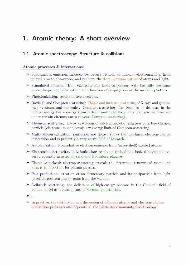
1.1. Atomic spectroscopy: Structure & collisions

Atomic processes & interactions:

➣ Spontaneous emission/fluorescence: occurs without an ambient electromagnetic field;related also to absorption, and it shows the deep quantum nature of atoms and light.

➣ Stimulated emission: from excited atoms leads to photons with basically the samephase, frequency, polarization, and direction of propagation as the incident photons.

➣ Photoionization: results in free electrons.

➣ Rayleigh and Compton scattering: Elastic and inelastic scattering of X-rays and gammarays by atoms and molecules. Compton scattering often leads to an decrease in thephoton energy but a energy transfer from matter to the photon can also be observedunder certain circumstances (inverse Compton scattering).

➣ Thomson scattering: elastic scattering of electromagnetic radiation by a free chargedparticle (electrons, muons, ions); low-energy limit of Compton scattering.

➣ Multi-photon excitation, ionization and decay: shows the non-linear electron-photoninteraction and is presently a very active field of research.

➣ Autoionization: Nonradiative electron emission from (inner-shell) excited atoms.

➣ Electron-impact excitation & ionization: results in excited and ionized atoms and oc-curs frequently in astro-physical and laboratory plasmas.

➣ Elastic & inelastic electron scattering: reveals the electronic structure of atoms andions; it is important for plasma physics.

➣ Pair production: creation of an elementary particle and its antiparticle from light(electron-positron pairs); pairs from the vacuum.

➣ Delbruck scattering: the deflection of high-energy photons in the Coulomb field ofatomic nuclei as a consequence of vacuum polarization.

➣ ...

➣ In practice, the distinction and discussion of different atomic and electron-photoninteraction processes also depends on the particular community/spectroscopy.

7


1.2. Atomic theory

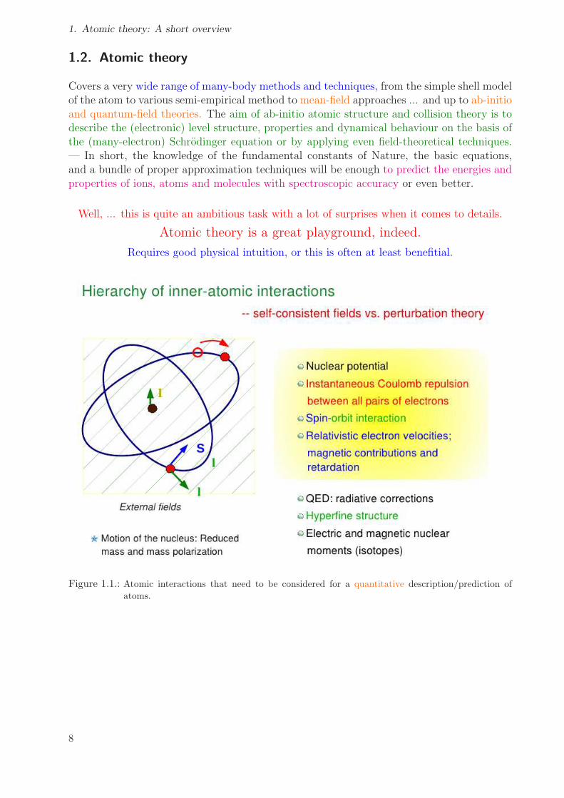
Covers a very wide range of many-body methods and techniques, from the simple shell modelof the atom to various semi-empirical method to mean-field approaches ... and up to ab-initioand quantum-field theories. The aim of ab-initio atomic structure and collision theory is todescribe the (electronic) level structure, properties and dynamical behaviour on the basis ofthe (many-electron) Schrodinger equation or by applying even field-theoretical techniques.— In short, the knowledge of the fundamental constants of Nature, the basic equations,and a bundle of proper approximation techniques will be enough to predict the energies andproperties of ions, atoms and molecules with spectroscopic accuracy or even better.

Well, ... this is quite an ambitious task with a lot of surprises when it comes to details.

Atomic theory is a great playground, indeed.

Requires good physical intuition, or this is often at least benefitial.

Figure 1.1.: Atomic interactions that need to be considered for a quantitative description/prediction of

atoms.

8

1.2. Atomic theory

Figure 1.2.: Characteristic time scales of atomic and molecular motions; taken from: Controlling the Quan-

tum World, page 99.

Theoretical models:

➣ Electronic structure of atoms and ions: is described quantum mechanically in termsof wave functions, energy levels, ground-state densities, etc., and is usually based onsome atomic (many-electron) Hamiltonian.

➣ Interaction of atoms with the radiation field: While the matter is treated quantum-mechanically, the radiation is — more often than not (> 99 % of all case studies) —described as a classical field (upon which the quantum system does not couple back).

➣ This semi-classical treatment is suitable for a very large class of problems, sometimesby including quantum effects of the field in some ‘ad-hoc’ manner (for instance,spontaneous emission).

➣ Full quantum treatment: of the radiation field is very rare in atomic and plasma physicsand requires to use quantum-field theoretical techniques; for example, atomic quantumelectrodynamics (QED). QED is important for problems with definite photon statisticsor in cavities in order to describe single-photon-single-atom interactions.

9


Combination of different (theoretical) techniques:

➣ Special functions from mathematical physics (spherical harmonics, Gaussian, Legendre-and Laguerre polynomials, Whittacker functions, etc.).

➣ Racah’s algebra: Quantum theory of angular momentum.

➣ Group theory and spherical tensors.

➣ Many-body perturbation theory (MBPT, coupled-cluster theory, all-order methods).

➣ Multiconfigurational expansions (CI, MCDF).

➣ Density matrix theory.

➣ Green’s functions.

➣ Advanced computational techniques (object-oriented; computer algebra;high-performance computing).

1.3. Applications of atomic theory

1.3.a. Need of (accurate) atomic theory and data

➣ Astro physics: Analysis and interpretation of optical and x-ray spectra.

➣ Plasma physics: Diagnostics and dynamics of plasma; astro-physical, fusion or labora-tory plasma.

➣ EUV lithography: Development of UV/EUV light sources and lithograhpic techniques(13.5 nm).

➣ Atomic clocks: design of new frequency standards; requires very accurate data onhyperfine structures, atomic polarizibilities, light shift, blackbody radiation, etc.

➣ Search for super-heavy elements: beyond fermium (Z = 100); ‘island of stability’; betterunderstanding of nuclear structures and stabilities.

➣ Nuclear physics: Accurate hyperfine structures and isotope shifts to determine nuclearparameters; formation of the medium and heavy elements.

➣ Surface & environmental physics: Attenuation, autoionization and light scattering.

➣ X-ray science: Ion recombination and photon emission; multi-photon processes; devel-opment of x-ray lasers; high-harmonic generation (HHG).

➣ Fundamental physics: Study of parity-nonconserving interactions; electric-dipole mo-ments of neutrons, electrons and atoms; ‘new physics’ that goes beyond the standardmodel.

➣ Quantum theory: ‘complete’ experiments; understanding the frame and boundaries ofquantum mechanics ?

➣ ...

10

1.4. Overview to light-matter interactions

1.3.b. Laser-particle acceleration: An alternative route

➣ High power short-pulse lasers with peak powers at the Terawatt or even Petawattlevel enables one to reach focal intensities of 1018 − 1023 W/cm2. These lasers areable also to produce a variety of secondary radiation, from relativistic electrons andmulti-MeV/nucleon ions to high energetic x-rays and gamma-rays.

➣ Applications: The development of this novel tool of particle acceleration is presentlyexplored in many different labs, and includes studies in fundamental and high-fieldphysics as well as on medical technologies for diagnostics and tumor therapy.

➣ Extreme Light Infrastructure (ELI): a new EU-funded large-scale research infrastruc-ture in which one (out of four) pillar is exclusively devoted to nuclear physics basedon high intensity lasers. The aim is to push the limits of laser intensity three orderstowards 1024 W/cm2.

➣ This ELI project, a collaboration of 13 European countries, comprises three branches:

• Ultra High Field Science to explore laser-matter interactions in an energy range where relativistic

laws could stop to be valid;

• Attosecond Laser Science to conduct temporal investigations of the electron dynamics in atoms,

molecules, plasmas and solids at the attosecond scale;

• High Energy Beam Science.

Figure 1.3.: Status of the ELI project 2014 (from: http://www.nature.com).

11


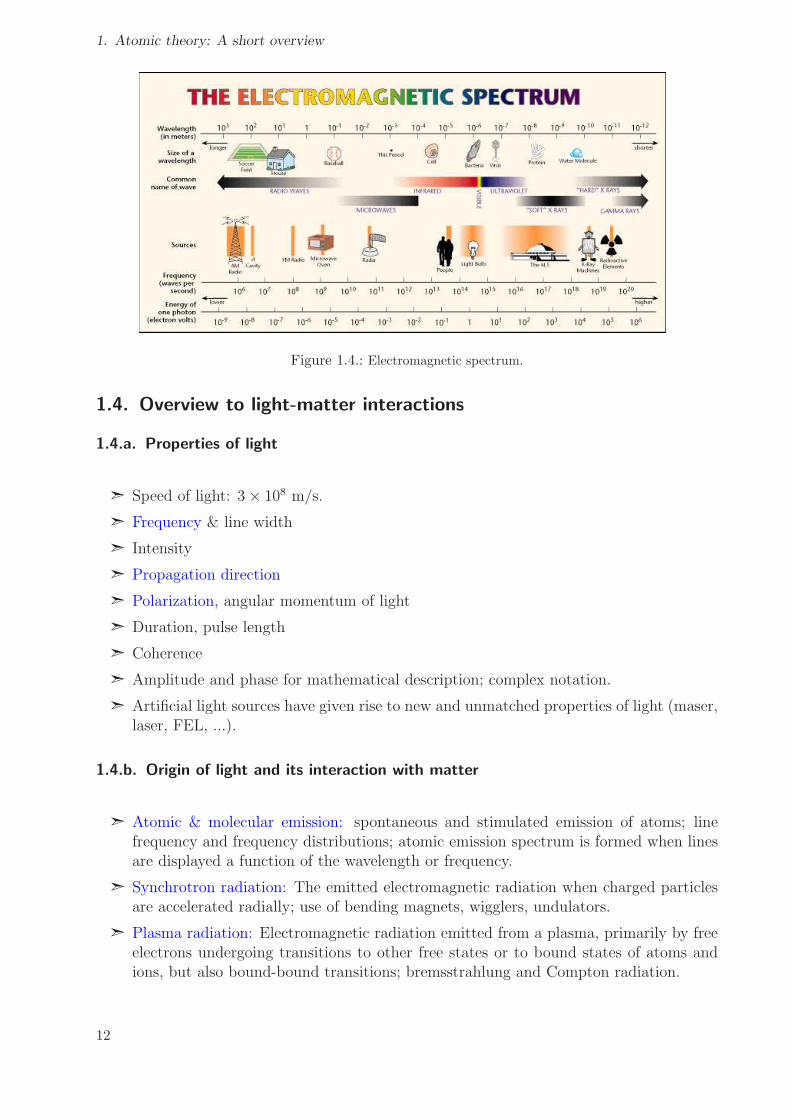
Figure 1.4.: Electromagnetic spectrum.


1.4.a. Properties of light

➣ Speed of light: 3× 108 m/s.

➣ Frequency & line width

➣ Intensity

➣ Propagation direction

➣ Polarization, angular momentum of light

➣ Duration, pulse length

➣ Coherence

➣ Amplitude and phase for mathematical description; complex notation.

➣ Artificial light sources have given rise to new and unmatched properties of light (maser,laser, FEL, ...).

1.4.b. Origin of light and its interaction with matter

➣ Atomic & molecular emission: spontaneous and stimulated emission of atoms; linefrequency and frequency distributions; atomic emission spectrum is formed when linesare displayed a function of the wavelength or frequency.

➣ Synchrotron radiation: The emitted electromagnetic radiation when charged particlesare accelerated radially; use of bending magnets, wigglers, undulators.

➣ Plasma radiation: Electromagnetic radiation emitted from a plasma, primarily by freeelectrons undergoing transitions to other free states or to bound states of atoms andions, but also bound-bound transitions; bremsstrahlung and Compton radiation.

12


➣ Blackbody radiation: best possible emitter of thermal radiation which results in acharacteristic, continuous spectrum that depends on the body’s temperature. As thetemperature increases beyond a few hundred degrees Celsius, black bodies start to emitvisible wavelengths, appearing red, orange, yellow, white, and blue with increasingtemperature. Planck’s law; Rayleigh-Jeans law.

Interactions of light with atoms and matter:

➣ Light can also undergo reflection, scattering and absorption; sometimes, the en-ergy/heat transfer through a material is mostly radiative, i.e. by emission and ab-sorption of photons (for example, in the core of the Sun).

➣ Light of different frequencies may travel through matter at different speeds; this iscalled dispersion. In some cases, it can result in extremely slow speeds of light inmatter slow light.

➣ The factor by which the speed of light is decreased in a material is called the refractiveindex of the material. In a classical wave picture, the slowing can be explained by thelight inducing electric polarization in the matter; the polarized matter then radiatesnew light, and the new light interfers with the original light wave to form a delayedwave.

➣ Alternatively, photons may be viewed as always traveling at c, even in matter. Dueto the interaction atomic scatters, the photons get a shifted (delayed or advanced)phase. In this bare-photon picture, photons are scattered and phase shifted, whilein the dressed-state photon picture, the photons are dressed by their interaction withmatter and move with lower speed but, otherwise, without scattering or phase shifts.

➣ Nonlinear optical processes are another active research area, including topics suchas two-photon absorption, self-phase modulation, and optical parametric oscillators.Though these processes are often explained in the photon picture, they do not requirethe assumption of photons. These processes are often modeled by treating some atomsor molecules as nonlinear oscillators.

➣ Light-matter interactions:

dispersion ➥ frequency spectrumdiffraction ➥ spatial frequency spectrumabsorption ➥ central frequencyscattering ➥ change in wavelength

Different approaches for studying light-matter interactions:

➣ Geometrical optics: λ ≪ object size ➥ daily experience;optical instrumentation; optical imaging.intensity, direction, coherence, phase, polarization, photons

➣ Wave optics: λ ≈ object size ➥ interference, diffraction, dispersion, coherence;laser, resolution issues, pulse propagation, holography.intensity, direction, coherence, phase, polarization, photons

➣ Laser and electro-optics: reflection and transmission in wave guides; resonators, ...lasers, integrated optics, photonic crystals, Bragg mirrors, ...intensity, direction, coherence, phase, polarization, photons

13


➣ Quantum optics: photons and photon number statistics, fluctuation, atoms in cavities,laser cooling techniques ...intensity, direction, coherence, phase, polarization, photons

1.4.c. Light sources

Traditional light sources:

➣ Celestial and atmospheric light: Sun, stars, aurorae, Cherenkov, ...

➣ Terrestrial sources: bioluminiscence (glowworm), volcanic (lava, ...)

➣ Combustion-based: candles, latern, argon flash, ...

➣ Electric-powered: halogen lamps, ...

➣ Gas discharge lamps: neon and argon lamps; mercury-vapor lamps, ...

➣ Laser & laser diodes: gas, semi-conductor, organic, ...

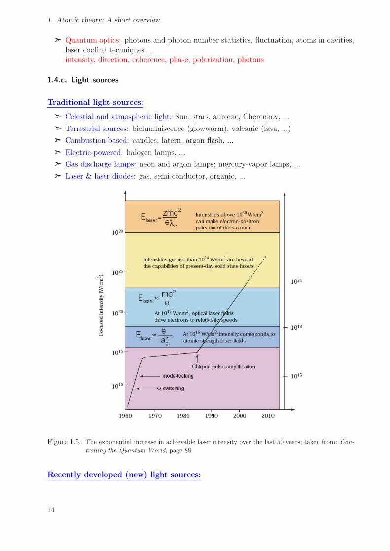
Figure 1.5.: The exponential increase in achievable laser intensity over the last 50 years; taken from: Con-

trolling the Quantum World, page 88.

Recently developed (new) light sources:

14


Figure 1.6.: Left: Photonic crystals from nature. Right: Photonic crystals from artifical nanostructures.

➣ LED’s: Semiconductor diodes that consists out of a chip of semi-conducting materialand a p-n (positive-negative) junction. When connected to a power source, the currentflows from the p- to the n-side. LED’s generate little or no long wave IR or UV, butconvert only 15-25 % of the power into visible light; the remainder is converted toheat that must be conducted from the LED die (p-n junction) to the underlying circuitboard and heat sinks.

➣ Laser-plama light sources: The application of a dense plasma focus as a light sourcefor extreme ultraviolet (EUV) lithography.

➣ High-harmomic generation (HHG): tunable table-top source of XUV/Soft X-rays thatis usually synchronised with the driving laser and produced with the same repetitionrate; HHG strongly depends on the driving laser field and, therefore, the high harmonicshave similar temporal and spatial coherence properties.

➣ Free-electron lasers (FEL): use a relativistic electron beam as the lasing medium whichmoves freely through a magnetic structure. FEL’s can cover a very wide frequency rangeand are well tunable, ranging currently from microwaves, through terahertz radiationand infrared, to the visible spectrum, to ultraviolet, to X-rays.

Further reading (Attosecond Light Sources):

➣ Read the article by David Villeneuve, La Physique au Canada 63 (2009) 65; cf. 1.2-Villeneuve.pdf on the web page of the lecture.

1.4.d. Atomic physics & photonics: Related areas and communities

➣ Spectroscopy: to study details of the medium, for instance, photon spectroscopy, elec-tron spectroscopy, Raman spectroscopy, ...Spectroscopic data are often represented by a spectrum, a plot of the response of in-terest as a function of wavelength or frequency.

➣ Different spectroscopic techniques are often distiguished by their type of radiative en-ergy (infrared-, x-ray-, etc.) nature of interaction (absorption-, emission-, coherent-,...) or type of materials (atoms, molecular, crystal, nuclei, ...).

15


Figure 1.7.: Left: The invisibility of meta materials. Right: Some 3d structures.

➣ Interferometry: family of techniques in which electromagnetic waves are superimposedin order to extract information about the waves and their properties. An instrumentused for that is called an interferometer. Interferometry is an important investiga-tive technique in the fields of astronomy, fiber optics, engineering metrology, opticalmetrology, oceanography, seismology, quantum mechanics, nuclear and particle physics,plasma physics, remote sensing and biomolecular interactions.

➣ Metrology: is the science of measurement. Metrology includes all theoretical and prac-tical aspects of measurement.

➣ Design of ‘new’ media: Photonic crystals are periodic optical nanostructures that aredesigned to affect the motion of photons in a similar way that periodicity of a semicon-ductor crystal affects the motion of electrons. Photonic crystals occur in nature and invarious forms.Meta materials are artificial materials engineered to have properties that may not befound in nature. Metamaterials usually gain their properties from structure rather thancomposition. Materials with negative refractive index; creation of superlenses whichmay have a spatial resolution below that of the wavelength; invisiblity and cloaking.

➣ Electro-magnetic optics: the study of the propagation and evolution of electromagneticwaves, including topics of interference and diffraction. Besides the usual branches ofanalysis, this area includes geometric topics such as the paths of light rays.

➣ Relativistic optics: The generation of ultrahigh intense pulse has open up a new fieldin optics, the field of relativistic nonlinear optics, where the nonlinearity is dictatedby the relativistic character of the electron. This young field has already produced aseries of landmark experiments. Among them are the generation of energetic beams ofparticles (electrons, protons, ions, positrons), as well as beams of X-rays and γ-rays.

➣ Quantum electronics: A term that is sometimes used for dealing with the effects ofquantum mechanics on the behavior of electrons in matter as well as their interactionswith photons. Nowadays, it is not seen so much as a sub-field of its own but has beenabsorbed into solid state physics, semiconductor physics, and several others.

16


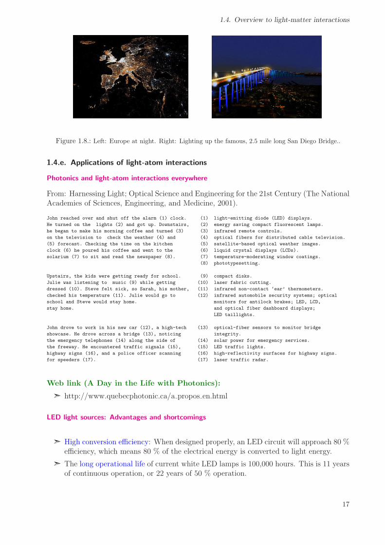
Figure 1.8.: Left: Europe at night. Right: Lighting up the famous, 2.5 mile long San Diego Bridge..

1.4.e. Applications of light-atom interactions

Photonics and light-atom interactions everywhere

From: Harnessing Light; Optical Science and Engineering for the 21st Century (The NationalAcademies of Sciences, Engineering, and Medicine, 2001).

John reached over and shut off the alarm (1) clock. (1) light-emitting diode (LED) displays.

He turned on the lights (2) and got up. Downstairs, (2) energy saving compact fluorescent lamps.

he began to make his morning coffee and turned (3) (3) infrared remote controls.

on the television to check the weather (4) and (4) optical fibers for distributed cable television.

(5) forecast. Checking the time on the kitchen (5) satellite-based optical weather images.

clock (6) he poured his coffee and went to the (6) liquid crystal displays (LCDs).

solarium (7) to sit and read the newspaper (8). (7) temperature-moderating window coatings.

(8) phototypesetting.

Upstairs, the kids were getting ready for school. (9) compact disks.

Julie was listening to music (9) while getting (10) laser fabric cutting.

dressed (10). Steve felt sick, so Sarah, his mother, (11) infrared non-contact ‘ear’ thermometers.

checked his temperature (11). Julie would go to (12) infrared automobile security systems; optical

school and Steve would stay home. monitors for antilock brakes; LED, LCD,

stay home. and optical fiber dashboard displays;

LED taillights.

John drove to work in his new car (12), a high-tech (13) optical-fiber sensors to monitor bridge

showcase. He drove across a bridge (13), noticing integrity.

the emergency telephones (14) along the side of (14) solar power for emergency services.

the freeway. He encountered traffic signals (15), (15) LED traffic lights.

highway signs (16), and a police officer scanning (16) high-reflectivity surfaces for highway signs.

for speeders (17). (17) laser traffic radar.

Web link (A Day in the Life with Photonics):

➣ http://www.quebecphotonic.ca/a propos en.html

LED light sources: Advantages and shortcomings

➣ High conversion efficiency: When designed properly, an LED circuit will approach 80 %efficiency, which means 80 % of the electrical energy is converted to light energy.

➣ The long operational life of current white LED lamps is 100,000 hours. This is 11 yearsof continuous operation, or 22 years of 50 % operation.

17


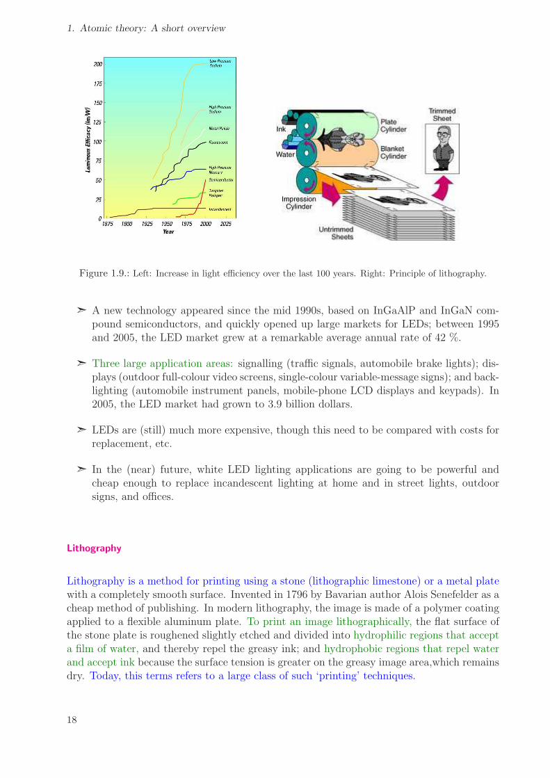
Figure 1.9.: Left: Increase in light efficiency over the last 100 years. Right: Principle of lithography.

➣ A new technology appeared since the mid 1990s, based on InGaAlP and InGaN com-pound semiconductors, and quickly opened up large markets for LEDs; between 1995and 2005, the LED market grew at a remarkable average annual rate of 42 %.

➣ Three large application areas: signalling (traffic signals, automobile brake lights); dis-plays (outdoor full-colour video screens, single-colour variable-message signs); and back-lighting (automobile instrument panels, mobile-phone LCD displays and keypads). In2005, the LED market had grown to 3.9 billion dollars.

➣ LEDs are (still) much more expensive, though this need to be compared with costs forreplacement, etc.

➣ In the (near) future, white LED lighting applications are going to be powerful andcheap enough to replace incandescent lighting at home and in street lights, outdoorsigns, and offices.

Lithography

Lithography is a method for printing using a stone (lithographic limestone) or a metal platewith a completely smooth surface. Invented in 1796 by Bavarian author Alois Senefelder as acheap method of publishing. In modern lithography, the image is made of a polymer coatingapplied to a flexible aluminum plate. To print an image lithographically, the flat surface ofthe stone plate is roughened slightly etched and divided into hydrophilic regions that accepta film of water, and thereby repel the greasy ink; and hydrophobic regions that repel waterand accept ink because the surface tension is greater on the greasy image area,which remainsdry. Today, this terms refers to a large class of such ‘printing’ techniques.

18


Figure 1.10.: The transatlantic cable system continues to grow.

Telecommunication, Medicine & life sciences

Sensorics

Micro- and nano-optics

19

2. Atoms in static external fields

Change of level structure and line spectra in external fields due to:

➣ Splitting of degnerate levels.

➣ Shift of energy levels.

➣ Superposition and hybridization of energy levels.

Usually, the level splitting in external fields is treated perturbatively by studying the

Hamiltonian: H = Ho + H ′.

2.1. Atoms in homogenoeus magnetic effects (Zeeman effect)

Splitting in external B -field due to:

➣ Particle with magnetic moment µµµ has energy: e = −µµµ ·B➣ Magnetic moment of electron due to its orbital angular momentum:

µµµl = − e�

2ml = −µB

l

�µB =

e�

2m... Bohr′s magneton .

➣ Spin magnetic moment: µµµs = − gse�2m

s = − gs µBs

�with gs = 2 (Dirac theory).

➣ g-factor: one of the most accurate quantities in physics; differs for free and boundelectrons and generally depends on the details of binding � gJ -factor of atomic levels.

➣ Total Hamiltonian (atom ’plus’ magnetic field):

H = − Δ

2− Z

r+ ξ(r) l · s

� ��

fine−structure, HFS

+ µB (l+ 2s) · B� ��

B−field interaction, HB

= Ho + HFS + µB (lz + 2sz) · Bz B || ez .

Often, one distinguishes three effects of a homogeneous magnetic field:

➣ Normal Zeeman effect: Splitting of atomic level (energies) with total spin S = 0 intousually three σ± and π -components.

➣ Anomalous Zeeman effect: Splitting of atomic level (energies) with total spin S �= 0.

➣ Paschen-Back effect: Limit of the anomalous Zeeman effect for strong fields, in whichthe spin-orbit coupling is broken by the external magnetic field.

21


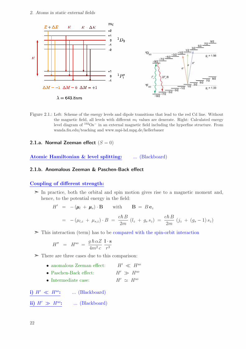
Figure 2.1.: Left: Scheme of the energy levels and dipole transitions that lead to the red Cd line. Without

the magnetic field, all levels with different ml values are denerate. Right: Calculated energy

level diagram of 192Os− in an external magnetic field including the hyperfine structure. From

wanda.fiu.edu/teaching and www.mpi-hd.mpg.de/kellerbauer

2.1.a. Normal Zeeman effect (S = 0)

Atomic Hamiltonian & level splitting: ... (Blackboard)

2.1.b. Anomalous Zeeman & Paschen-Back effect

Coupling of different strength:

➣ In practice, both the orbital and spin motion gives rise to a magnetic moment and,hence, to the potential energy in the field:

H ′ = − (µµµl + µµµs) ·B with B = B ez

= − (µl,z + µs,z) · B =e�B

2m(lz + gs sz) =

e�B

2m(jz + (gs − 1) sz)

➣ This interaction (term) has to be compared with the spin-orbit interaction

H ′′ = Hso =g �αZ

4m2 c

l · sr3

➣ There are three cases due to this comparison:

• anomalous Zeeman effect: H ′ ≪ Hso

• Paschen-Back effect: H ′ ≫ Hso

• Intermediate case: H ′ ≃ Hso

i) H ′ ≪ Hso: ... (Blackboard)

ii) H ′ ≫ Hso: ... (Blackboard)

22

2.2. Atoms in homogenoeus electric fields (Stark effect)

2.1.c. Zeeman effect for different field strengths B

With increasing field strength B : ... (Blackboard)


2.2.a. Linear Stark effect

Atom-field Hamiltonian: ... (Blackboard)

Figure 2.2.: he 1st excited state is split from 4 degenerate states to 2 distinct, and 1 degenerate state.

2.2.b. Quadratic Stark effect

Hydrogen in the 1s ground state: ... (Blackboard)

23


Figure 2.3.: Stark effect on the n = 2 → 3 transitions in atomic hydrogen. Left: The electric

field is said to be strong when the splitting of the energy levels becomes larger than the

fine-structure splitting. Right: The transition energy without the fine-structure. From

http://www.afs.enea.it/apruzzes/Spectr/Stark.

24


Figure 2.4.: The n = 2 → 3 transition energy including the fine-structure of the levels. From

http://www.afs.enea.it/apruzzes/Spectr/Stark.

25

3. Interactions of atoms in weak (light) fields

Basic assumption: Weak coupling of the atom with the radiation field, i.e. the field doesnot affect the electronic structure of the atoms and ions.

3.1. Radiative transitions

3.1.a. Einstein’s A and B coefficients

Consider two levels of an atom: �ω = E2 − E1 > 0.

Figure 3.1.: Model of the induced and spontaneous processes.

ρ(ω) ... energy density/dν =number of photons

volume · dν

Einstein’s argumentation and coefficients:

➣ Einstein’s rate equation

− dN2

dt=

dN1

dt� ��

particle conservation

= AN2 + B21 ρ(ω) N2 − B12 ρ(ω) N1

= Pemission N2 − Pabsorption N1

➣ No field, ρ(ω) = 0:

N2(t) = N2(0) e−At A =

1

τ

A ... inverse lifetime, transition rate [1/s]

27


➣ Equilibrium state: dN2

dt= 0:

Pabsorption

Pemission

=N2

N1

=B12 ρ(ω)

A + B21 ρ(ω)

➣ Atoms with more than two levels: We here assume additionally the principle of detailedbalance

Pij

Pji

=Nj

Ni

=Bij ρ(ωij)

Aji + Bji ρ(ωij)

For each pair ij of atomic levels, the emission and absorption is in equilibrium, andindependent of other possible transition processes.

➣ Generalized field-free case:

− dNj

dt=

�

i

AjiNj � τj =

��

i

Aji

�−1

➣ Ratio Aji : Bji : Bij:

Thermal equilibrium:

− Nj

Ni

=gjgi

exp

�

− �ωij

kT

�

g(ωij) =ω2ij

π2 c3�ωij

exp�

− �ωij

kT

�

− 1

Planck’s black-body radiation

➣ Einstein’s relation (1917): Relation of detailed balance is fulfilled for

Aji =ω2ij

π2 c3� ωij Bji =

ω2ij

π2 c3� ωij

gigj

Bij

Einstein’s coefficients depend on the internal structure of the atoms and they are (as-sumed to be) independent of the radiation field and the state of the atomic ensemble.

3.1.b. Additional material to Einstein relations and others

Some additions: ... (Blackboard)

Photoabsorption and emission of σ- vs. π-light ... (Blackboard)

Line-width contributions in atomic spectroscopy ... (Blackboard)

28

3.1. Radiative transitions

Example (Line-width contributions for the yellow sodium line): This ’yellow line’

(known from sodium vapor lamps, for instance) has the frequency ωo ∼ 2π · 4 · 1014 Hz, alifetime τ ∼ 10−8 s and a natural width Δωo ∼ 108 Hz.

For sodium with mass number A = 23 and for a temperature T = 500 K, we find a Dopplerwidth Δω/ω ∼ 3 · 10−6 or Δω ≈ 12 GHz.

In general: Doppler widths ≫ natural widts.

3.1.c. Transition amplitudes and probabilities

radiation field interaction atomic structure

(time− dependent) ⇐⇒ and motion

Time-dependent perturbation theory:

• semi-classical: quantized atom ⊕ classical em field.

• QED: quantized atom ⊕ quantized em field (Dirac 1927).

Limitations of the semi-classical description: ... (Blackboard)Hamiltonian function of a particle in an electro-magnetic field:

H =1

2m(p + eA)2 − eφ + V E = −∇∇∇φ − ∂A

∂t

B = rotA

(φ,A) ... 4− comp. vector potential

=p2

2m+ V (r) +

e

2m(p ·A + A · p) +

e2

2mA2 − eφ

= Hatom + Hatom−field interaction

= Ho + H ′

Special case: Superposition of plane waves

φ = 0

A = Ao ei (k·r−ωt) + A1 e

−i (k·r−ωt)

divA = 0 Coulomb gauge [p, A] = 0

H ′ =e

mA · p +

e2

2mA2

� ��

neglegible

29


Ho ⊕ time-dependent perturbation ➥ time-dependent perturbation theory.

Absorption probability: ... (Blackboard)

3.2. Electric-dipole interactions and higher multipoles

3.2.a. Electric-dipole approximation

Consider a light field with plane-wave structure ∼ eik·r and |k| = 2πλ;

➥ visible light: λ ≈ 500 nm ... 1000-10000 atomic radii

eik·r = 1 + ik · r + ...

Dipole approximation: light wave is constant over the extent of the atom.

Evaluation of the Einstein A coefficients: ... (Blackboard)

3.2.b. Selection rules and discussion

Intensity of lines ∼ (i) occpuation of levels; (ii) transition probability.

Electron temperature Te:

Nj

Ni

=gjgi

e−(Ej − Ei)

kT

• Te ≈ 104 K � kTe ∼ 1 eV

• Te ≈ 300 K � kTe ∼ 1/40 eV

• Te → ∞

Selection rules for bound-bound transitions: ... (Blackboard)

3.2.c. Higher multipole components

eik·r = 1 + ik · r + ...

magnetic-dipole (M1) and electric-quadrupole (E2) radiation

(M1) ∼ ω2

c2

��

�

j

��

e �

2mla

��i

��

2

=ω2

c2|�j |µµµla | i�|2

µµµ =e �

2ml ... magnetic moment of electron

(E2) ∼ ω4

c2|�j | e xaxb| i�|2

30

3.3. Multipol expansions of the radiation field

xaxb ... second-order tensor (components)

Intensity ratio for hydrogen-like wave functions:

E1 : M1 : E2 = 1 : α2 : α2

3.2.d. Dipole transitions in many-electron atoms

For a weak radiation field, its interaction with the atom can be described perturbatively bythe Hamiltonian

H ′ =e

mA ·

�

k

pk

and where the spontenous emission rates are obtained from the induced rates via the Einsteinrelation above. In this very common semi-classical approach, the spontenous emission ratesis

Aji =32 π3e2 a2o

3h(Ej − Ei)

3�

q

��γjJjMj

��P (1)

q

�� γiJiMi

��2

P (1)q =

N�

i=1

r(1)q (i) =N�

i=1

ri

�

4π

3Y1q(ϑi,ϕi)

spherical component of the (many-electron) dipole operator

Analogue formulas also applied for the multipole radiation of higher order.

Spherical tensor operators: ... (Blackboard)

Gauge forms of the transition probabilities: ... (Blackboard)

Selection rules for electric-dipole radiation: ... (Blackboard)

3.3. Multipol expansions of the radiation field

Multipoles ... ... (Blackboard)

31


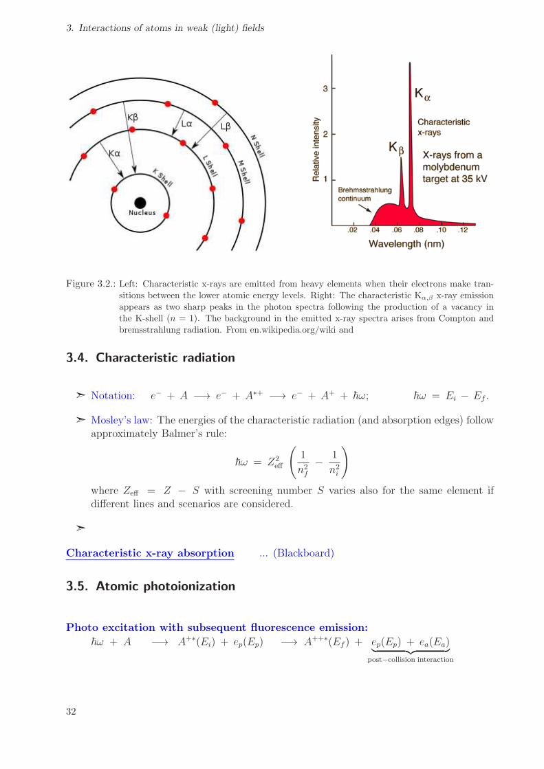
Figure 3.2.: Left: Characteristic x-rays are emitted from heavy elements when their electrons make tran-

sitions between the lower atomic energy levels. Right: The characteristic Kα,β x-ray emission

appears as two sharp peaks in the photon spectra following the production of a vacancy in

the K-shell (n = 1). The background in the emitted x-ray spectra arises from Compton and

bremsstrahlung radiation. From en.wikipedia.org/wiki and

3.4. Characteristic radiation

➣ Notation: e− + A −→ e− + A∗+ −→ e− + A+ + �ω; �ω = Ei − Ef .

➣ Mosley’s law: The energies of the characteristic radiation (and absorption edges) followapproximately Balmer’s rule:

�ω = Z2eff

�

1

n2f

− 1

n2i

�

where Zeff = Z − S with screening number S varies also for the same element ifdifferent lines and scenarios are considered.

➣

Characteristic x-ray absorption ... (Blackboard)

3.5. Atomic photoionization

Photo excitation with subsequent fluorescence emission:

�ω + A −→ A+∗(Ei) + ep(Ep) −→ A++∗(Ef ) + ep(Ep) + ea(Ea)� ��

post−collision interaction

32

3.6. Radiative electron capture

Figure 3.3.: While the x-ray (analytical) community still largely uses the so-called Siegbahn notation, the

IUPAC notation is consistent with notation used for Auger electron spectroscopy, though the

latter one is slightly more cumbersome. From nau.edu/cefns/labs

3.5.a. Photoionization amplitudes

➣ Photoionoization from the ground state for �ω > Ip (1st ionization potential.

➣ For a weak photon field, this ionization is again caused by the Hamiltonian

H ′ =e

mA ·

�

i

pi

➣ The (induced) photo excitation and ionization is usually described by means of crosssections:

σi→f (ω) ∼ ω3�

q

��(γfJf , ǫfκf )J

′M ′��P (1)

q

�� γiJiMi

��2.

3.6. Radiative electron capture

➣

e−(Ekin) + A −→ A+∗(Ei) + �ω −→

➣

33


Figure 3.4.: Left: Edges in the x-ray absorption coefficients as function of the photon energy. Right:

Principle of X-ray absorption near edge structure (XANES) and extended X-ray absorption

fine structure (EXAFS) spectroscopy. From chemwiki.ucdavis.edu and pubs.rsc.org

3.7. Bremsstrahlung

➣ e− + A =⇒ e− + A + γ

➣ Maximal electron energy Emax = eU leads to a minimum wave lengths

λmin =hc

Emax

=hc

eUλ[nm] =

1240

E[eV ] .

➣ Examples: U = 10kV � λ ∼ 1 A; U = 100kV � λ ∼ 0.1 A

3.8. Non-radiative transitions: Auger transitions and autoionization

➣ Auger transitions and autoionization are caused by the inter-electronic interactions.

➣ Kinetic energy of emitted electrons:

Ekin = E(initial, N) − E(final, N − 1)

➣ Autoionization: (Low-energy) emission of valence electrons.

Auger decay: (High-energetic) electron emission after decay of an inner-shellhole.

➣ Autoionization and Auger decay are theoretically ver similar; they are both describedby the Auger rate

Afi ∼ 2π

��

�

(γfJf , ǫfκf )J′M ′

��

�

i<j

1

rij

��γiJiMi

��

2

34

3.9. Beyond single-photon or single-electron transitions

Figure 3.5.: The total absorption coefficient of lead (atomic number 82) for gamma rays, plotted versus

gamma energy, and the contributions by the three effects. Above 5 MeV, pair production

starts to dominate.

➣ Selection rules for Auger transitions:

ΔJ = ΔM = 0 (strict)

ΔL = ΔML = ΔS = ΔMS = 0 (in the non− relativistic framework)

➣ Excitation and subsequent decay:

�ω + A → A+∗(Ei) + ep(Ep) → A++∗(Ef ) + ep(Ep) + ea(Ea)� ��

post−collision interaction


Weak processes with several photons and/or electrons: ... (Blackboard)

35


Figure 3.6.: Comparison of different ionization and subsequent decay processes in atoms.

Figure 3.7.: First ionization potential as function of the nuclear charge of elements.

36


Figure 3.8.: Cross sections for photoionization of neutral W atoms. The upper panel shows the result of

relativistic Hartree-Fock (RHF) calculations for photoabsorption by neutral tungsten atoms

brought into the gas phase by evaporating tungsten at 3200 K. From www.mdpi.com.

Figure 3.9.: Left: Different elastic and inelastic electron scattering processes on atoms, including

bremsstrahlung. Right: Bremsstrahlung is characterized by a continuous distribution of ra-

diation that is shifted towards higher photon energies and becomes more intense with in-

creasing electron energy. From: www.nde-ed.org/EducationResources and hyperphysics.phy-

astr.gsu.edu

37


Figure 3.10.: Schematic diagram for the XPS emission process (left). An incoming photon causes the

ejection of the photoelectron. Relaxation process (right) resulting in the emission of an Auger

KLL electron; from http://www.vub.ac.be/

Figure 3.11.: Information Available from Auger electron spectroscopy. From and

http://www.lpdlabservices.co.uk

38


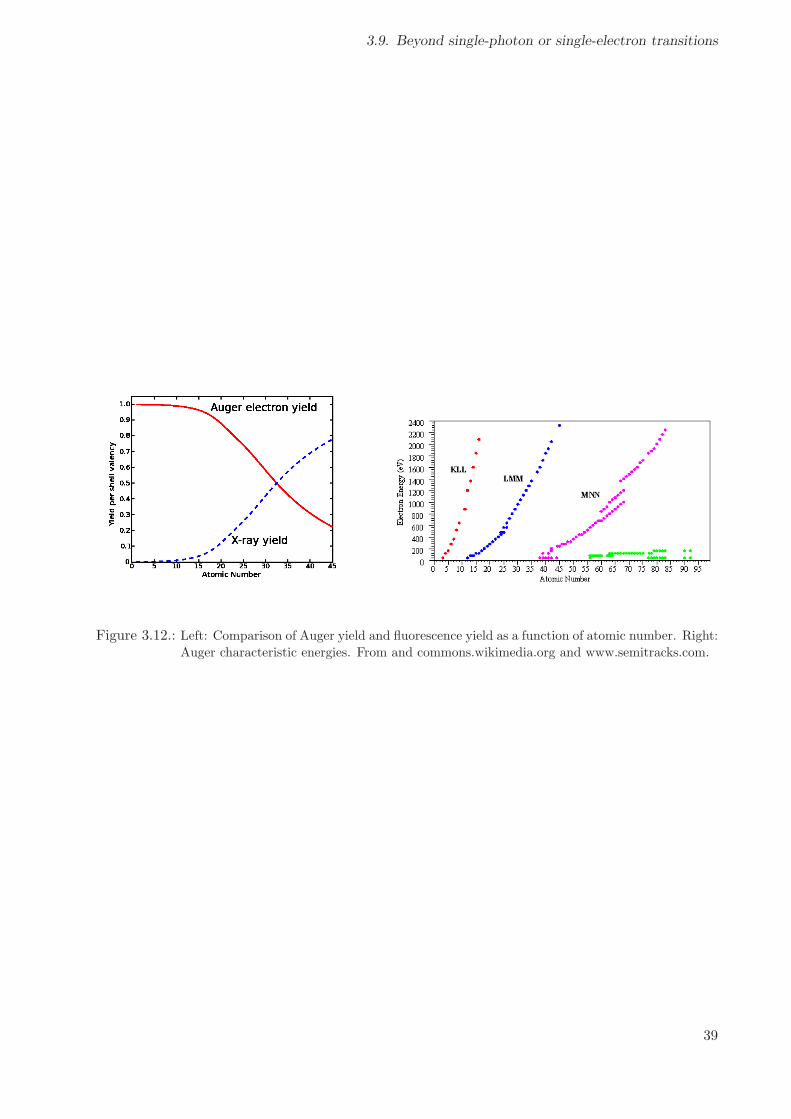
Figure 3.12.: Left: Comparison of Auger yield and fluorescence yield as a function of atomic number. Right:

Auger characteristic energies. From and commons.wikimedia.org and www.semitracks.com.

39

4. Interaction of atoms with driving light fields

Web link (Lecture by the nobel laureate Claude Cohen-Tannoudji):

➣ For more motivation, listen to cdsweb.cern.ch/record/423817

4.1. Time-dependent Schrodinger eq. for two-level atoms

Let us consider the time-dependent Schrodinger equation with H = H0+HI(t) , where H0

is the Hamiltonian of the free (unperturbed) atom and HI(t) describes the interaction withthe oscillating electric field.

For a finite set of levels with energy En, the eigenfunctions can be written as

Ψn(r, t) = ψn(r) e−

i�Ent .

For a two-level atom, that evolves under the influence of a perturbation HI(t), the time-dependent wave function can therefore be written as

Ψ(r, t) = c1(t)ψ1(r) e−

i�E1t + c2(t)ψ2(r) e

−i�E2t

= c1 |1� e−iω1t + c2 |2� e−iω2t

with ci ≡ ci(t) and ωi = Ei/� , and with |c1|2 + |c2|2 = 1 due to normalization.

Perturbation due to an oscillating electric field:

➣ For a bound electron e with position vector r (with regard to the center of mass), anoscillating electric field E = E0 cosωt gives rise to the Hamiltonian

HI(t) = e r · E0 cos(ωt)

➣ Substitution of ansatz Ψ(r, t) into the time-dependent SE gives

i c1 = Ω cos(ωt) e−ω0t c2 i c2 = Ω∗ cos(ωt) eω0t c1

with ω0 = (E2 − E1)/� and the (so-called) Rabi-frequency Ω.

➣ Rabi-frequency

Ω =�1 |er · E0| 2�

�=

e

�

�

d3rψ∗

1(r) r · E0 ψ2(r)

≈ eE0

�

�

d3rψ∗

1(r) rψ2(r)

41


➣ The dipole approximation in the last line holds when the radiation has a wavelengthgreater than the size of the atom, i.e. λ ≫ a0.

➣ Especially for linear-polarized radiation along x−axis, i.e. E = E0 ex cos(ωt):

Ω =eX12E0

�with X12 = �1 |x| 2� .

➣ In general, further approximations are needed to solve Eqs. (4.1) for c1(t) and c2(t).

Consider the initial (population) condition c1(0) = 1 and c2(0) = 0, a reasonable ‘first-order’solution is

c1(t) = 1

c2(t) =Ω∗

2

�1 + exp [i(ω0 + ω) t]

ω0 + ω+

1 + exp [i(ω0 − ω) t]

ω0 − ω

�

i.e. as long as c2(t) remains small.

Rotating-wave approximation: ... (Blackboard)

Figure 4.1.: The excitation probability function of the radiation frequency has a maximum at the atomic

resonance. The line width is inversely proportional to the interaction time; from Foot (2006).

4.2. Einstein’s B coefficient revisited

So far, we considered the effect of an oscillating electric field E0 cos(ωt) on the atom. Howis this (quantum-mechanial) behavior of the excitation probability related to Einstein’s sta-tistical treatment of the atom-field interaction ? Especially, what do we expect if somebroadband radiation with the energy density ρ(ω) dω = ǫ0 E

20(ω)/2 interacts with a

two-level atom ?

Einstein’s coefficients expressed by the dipole amplitude:

42

4.2. Einstein’s B coefficient revisited

➣ If we square the Rabi frequency Ω for linear-polarized radiation and use the energydensity from above, we find

|Ω|2 =

��

eX12 E0(ω)

�

��

2

=e2 |X12|2

�2

2ρ(ω) dω

ǫ0,

and together with c2(t) (by integration over the frequency)

|c2(t)|2 =2e2 |X12|2

ǫ0 �2

� ω0+Δ/2

ω0−Δ/2

dω ρ(ω)sin2{(ω0 − ω)t/2}

(ω0 − ω)2.

This is the excitation probability for broadband radiation.

➣ This expression for the makes use of the assumption that contributions at differentfrequencies do not interfere with each other.

➣ Since for broadband radiation, the energy density ρ(ω) does not change significantlyover the ‘major’ extent of the sinc-function, one can take the density out of the integraland write

|c2(t)|2 ≃ 2e2 |X12|2ǫ0 �2

ρ(ω0) × t

2

� φ

−φ

dxsin2x

x2.

steady-state excitation rate for broadband radiation

Apparently, the probability for a transition from level 1 to 2 increases linearly withtime.

➣ Steady-state excitation rate for broadband radiation: This rate (i.e. the transitionprobability per time) is given by

R12 =|c2(t)|2

t=

e2 |X12|2ǫ0 �2

.

➣ Comparison with Einstein’s treatment of the upward rate, B12 ρ(ω0) shows:

B12 =πe2|D12|23ǫ0�2

,

if we replace |X12|2 −→ |D12|2/3, i.e. by the (magnitude of the) standard dipole matrixelement

D12 = �1 |r| 2� =

�

d3r ψ∗

1 rψ2 .

➣ Here, D12 is a vector, and the factor 1/3 arises from the average of D · erad (with eradbeing the unit vector along the electric field) over all spatial directions.

➣ From the known relation between the Einstein coefficients A21 and B21, we finally find

A12 =g1g2

4α

3c2× ω3 |D12|2

where α = e2/4πǫ0 �c is the fine-structure constant. The matrix element D12 betweenthe initial and final states depends only on the wave functions of the atom, that is theEinstein coefficients are properties of the atom or molecule.

43


➣ For some typical (allowed) transition, the matrix element above has a value D12 ≃ 3a0(taking the wave functions from hydrogen), and this gives A21 ≃ 2π × 107/s−1 for atransition of the wavelength λ = 6× 10−7 m and g1 = g2 = 1.

In conclusion, although we have no real explanation for the spontaneous emission of atomsand molecules, Einstein’s treatment provides us with a relation between A21 and B21, andwe have used time-dependent perturbation theory to derive an expression for B21.

4.3. Interaction of atoms with monochromatic radiation

4.3.a. Rabi oscillations

➣ If c2(t) is not small for all times, we re-write Eq. (4.1) as:

ic1 = c2�ei(ω−ω0)t + e−i(ω+ω0)t

� Ω

2

and analogue for ic2.

➣ Since the term (ω + ω0)t oscillates very quickly, it averages to zero for any reasonableinteraction time, and we obtain a second-order differential equation for c2(t):

d2c2dt2

+ i(ω − ω0)dc2dt

+

��

Ω

2

��

2

c2 = 0 .

➣ This initial-value equations can be solved for the conditions c1(0) = 1 and c2(0) = 0

|c2(t)|2 =Ω2

W 2sin2

�Wt

2

�

with W 2 = Ω2 + (ω − ω0)2

➣ At resonance (ω = ω0), we find

|c2(t)|2 = sin2

�Ωt

2

�

Rabi oscillations, i.e. the population oscillates between the two levels.

➣ When Ωt = π, all the population has gone from level 1 into the upper state, |c2(t)|2 = 1,and when Ωt = 2π the atom has returned back to the lower state.

π− and π/2−pulses: ... (Blackboard)

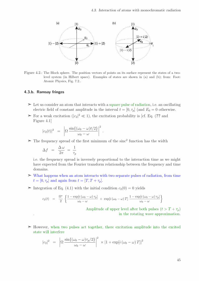
Bloch sphere representation: ... (Blackboard)

Web link (how a pulse acts upon a two-level atom):

➣ www.youtube.com/watch?v=eONhmaVKw c

➣ www.youtube.com/watch?v=n4iIx8XuJlU

44

4.3. Interaction of atoms with monochromatic radiation

Figure 4.2.: The Bloch sphere. The position vectors of points on its surface represent the states of a two-

level system (in Hilbert space). Examples of states are shown in (a) and (b); from: Foot:

Atomic Physics, Fig. 7.2..

4.3.b. Ramsay fringes

➣ Let us consider an atom that interacts with a square pulse of radiation, i.e. an oscillatingelectric field of constant amplitude in the interval t = [0, τp] (and E0 = 0 otherwise.

➣ For a weak excitation (|c2|2 ≪ 1), the excitation probability is [cf. Eq. (?? andFigure 4.1]

|c2(t)|2 =

��Ω

sin{(ω0 − ω)t/2}ω0 − ω

��

2

.

➣ The frequency spread of the first minimum of the sinc2 function has the width

Δf =Δω

2π=

1

τp

i.e. the frequency spread is inversely proportional to the interaction time as we mighthave expected from the Fourier transform relationship between the frequency and timedomains.

➣ What happens when an atom interacts with two separate pulses of radiation, from timet = [0, τp] and again from t = [T, T + τp].

➣ Integration of Eq. (4.1) with the initial condition c2(0) = 0 yields

c2(t) =Ω∗

2

�1− exp[i (ω0 − ω) τp]

ω0 − ω+ exp[i (ω0 − ω)T ]

1− exp[i (ω0 − ω) τp]

ω0 − ω

�

Amplitude of upper level after both pulses (t > T + τp). in the rotating wave approximation.

➣ However, when two pulses act together, there excitation amplitude into the excitedstate will interfere

|c2|2 =

��Ω

sin{(ω0 − ω)τp/2}ω0 − ω

��

2

× |1 + exp[i (ω0 − ω)T ]|2

45


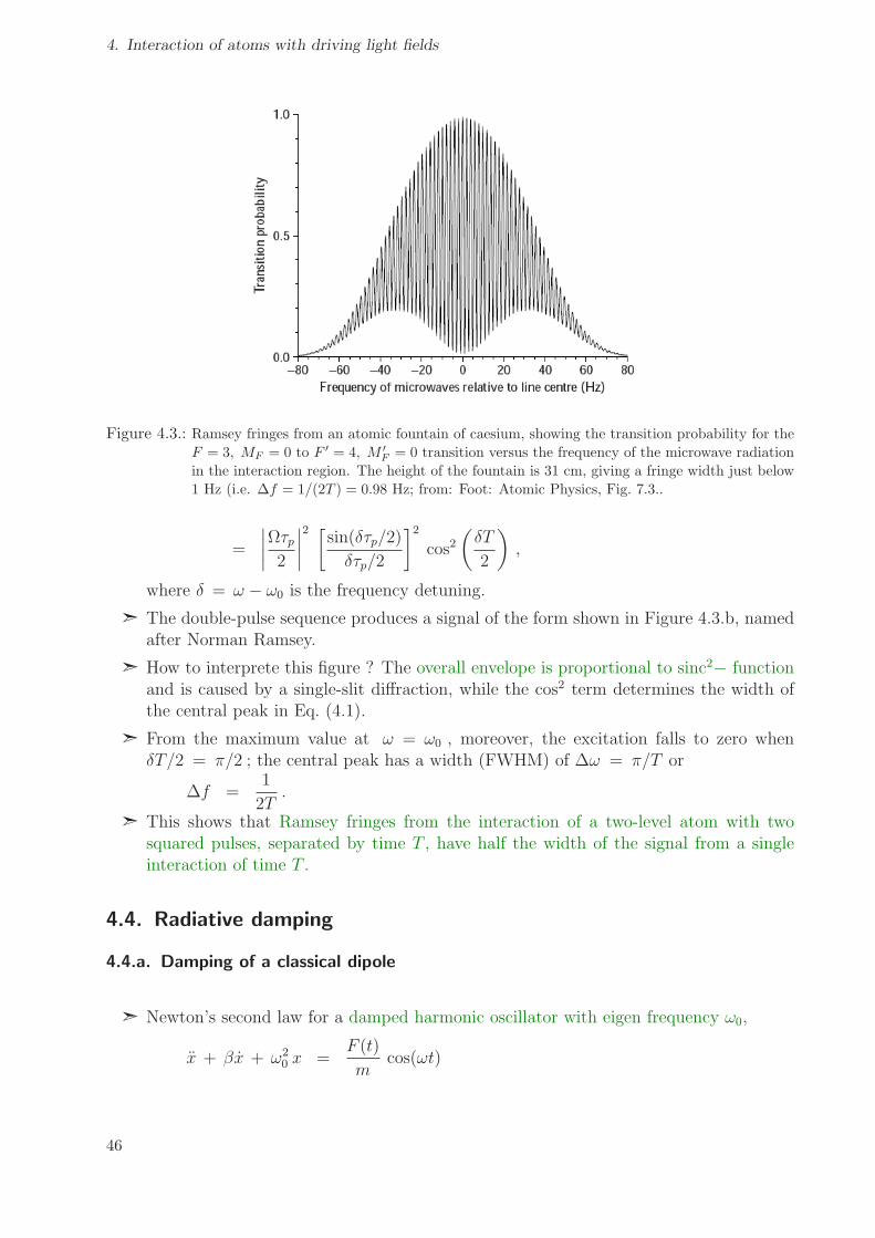
Figure 4.3.: Ramsey fringes from an atomic fountain of caesium, showing the transition probability for the

F = 3, MF = 0 to F ′ = 4, M ′

F = 0 transition versus the frequency of the microwave radiation

in the interaction region. The height of the fountain is 31 cm, giving a fringe width just below

1 Hz (i.e. Δf = 1/(2T ) = 0.98 Hz; from: Foot: Atomic Physics, Fig. 7.3..

=

��

Ωτp2

��

2 �sin(δτp/2)

δτp/2

�2

cos2�δT

2

�

,

where δ = ω − ω0 is the frequency detuning.

➣ The double-pulse sequence produces a signal of the form shown in Figure 4.3.b, namedafter Norman Ramsey.

➣ How to interprete this figure ? The overall envelope is proportional to sinc2− functionand is caused by a single-slit diffraction, while the cos2 term determines the width ofthe central peak in Eq. (4.1).

➣ From the maximum value at ω = ω0 , moreover, the excitation falls to zero whenδT/2 = π/2 ; the central peak has a width (FWHM) of Δω = π/T or

Δf =1

2T.

➣ This shows that Ramsey fringes from the interaction of a two-level atom with twosquared pulses, separated by time T , have half the width of the signal from a singleinteraction of time T .

4.4. Radiative damping

4.4.a. Damping of a classical dipole

➣ Newton’s second law for a damped harmonic oscillator with eigen frequency ω0,

x + βx + ω20 x =

F (t)

mcos(ωt)

46

4.4. Radiative damping

for a driving frequency ω and a friction force F friction = −mβ x . The amplitude ofF (t) is assumed to vary slowly when compared with ω.

➣ Solution can be found with ansatz, see classical mechanics:

x(t) = U(t) cosωt − V(t) sinωt .

➣ For (F (t) = 0), i.e. no driving force, we obtain

x(t) = x0 e−βt/2 cos(ω′t + φ)

with ω′ ≃ ω0 for light damping β/ω0 ≪ 1. The energy is proportional to the amplitudeof the motion squared, E ∝ exp(−βt).

➣ For a (nearly) constant driving force (F (t) =, the energy of the classical oscillator

E =|FV|ω2β

increases linearly with the strength of the driving force.

➣ In a two-level atom, in contrast, the energy must have an upper limit

4.4.b. Density matrix of a two-level system

For a semi-classical description of an atom in the radiation field, we need to know the electricdipole moment of the atom as induced by the radiation

−eDx(t) = −�

d3rΨ+(t) exΨ(t) .

(Optical) Bloch equations:

➣ The electric dipole moment of the two-level atom can be either in terms of the (time-dependent) amplitudes c1(t), c2(t) or by means of the density matrix

|Ψ� �Ψ| =

�

c1

c2

�

�c∗1 c∗2

�=

�

|c1|2 c1c∗

2

c∗1c2 |c2|2

�

=

�

ρ11 ρ12

ρ21 ρ22

�

.

➣ In the density matrix, the diagonal elements |c1|2 and |c2|2 represent the (level) pop-ulation, while the off-diagonal matrix elements are (sometimes) called the coherenceswhich describe the response of the system to the frequency of the driving fields.

➣ In the expression of the electric dipole moment, the (modified) coherences appear in theform ρ12 = ρ12 exp(−iδt) with δ = ω− ω0 as well as ρ21 = ρ21 exp(iδt) = (ρ12)

∗ .

➣ With these definitions (of combined density matrix elements), the Schrodinger equa-tionfor the driven two-level atoms can be expressed in the compact form

u = δ v

v = −δ u + Ωω

w = −Ω v

(optical) Bloch equations

47


➣ In these Bloch equations, the three real and time-dependent functions are defined as

u = ρ12 + ρ21

v = −i(ρ12 − ρ21)

w = ρ11 − ρ22

i.e. as the real and imaginary parts of the density matrix.

➣ In addition, these three functions can be interpreted also as components of the (so-called) Bloch vector

R = u e1 + v e2 + w e3

(Optical) Bloch equations with damping: ... (Blackboard)

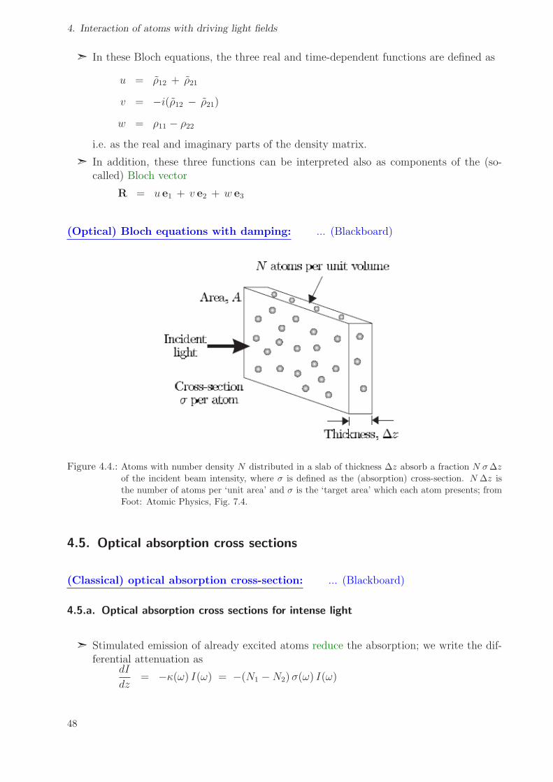
Figure 4.4.: Atoms with number density N distributed in a slab of thickness Δz absorb a fraction N σΔz

of the incident beam intensity, where σ is defined as the (absorption) cross-section. N Δz is

the number of atoms per ‘unit area’ and σ is the ‘target area’ which each atom presents; from

Foot: Atomic Physics, Fig. 7.4.

4.5. Optical absorption cross sections

(Classical) optical absorption cross-section: ... (Blackboard)

4.5.a. Optical absorption cross sections for intense light

➣ Stimulated emission of already excited atoms reduce the absorption; we write the dif-ferential attenuation as

dI

dz= −κ(ω) I(ω) = −(N1 −N2) σ(ω) I(ω)

48

4.5. Optical absorption cross sections

since absorption and stimulated emission have the same cross-section (see Einstein’sanalysis).

➣ In steady state, the conservation of energy further requires

(N1 −N2) σ(ω) I(ω) = N2 A21 �ω ,

because the net rate of the absorbed energy per unit volume (lhs) must be equal to therate of spontaneous emission times �ω (rhs).

➣ Since w = N2−N1

N, we can write the absorption cross section as

σ(ω) =ρ22w

A21 �ω

I=

Ω2/4

(ω − ω0)2 + Γ2/4× A21 �ω

I

= 3× π2c2

ω20

A21 gL(ω) (4.1)

➣ The particular frequency dependence is described by the (normalized) Lorentzian lineshape

gL(ω) =1

2π

Γ

(ω − ω0)2 + Γ2/4;

➣ The pre-factor (3) in (4.1) can take any value between 0 ... 3; for unpolarized light andrandomly oriented atoms, this factor is 1.

➣ Under these conditions and for denegerate levels, the optical absorption cross sectionbecome

σ(ω) =g2g1

× π2c2

ω20

A21 gL(ω)

Example (Zeeman level MF interacts with polarized laser beam): Consider

atoms in a specific MF state and a polarized laser beam, e.g. sodium atoms in a magnetictrap that absorb a circularly polarized probe beam, Figure 4.5.a.

To drive the ΔMF = +1 transition, we need circularly polarized light and a beam directionparallel to the quantization axis of the atoms (magnetic field).

4.5.b. Cross sections for pure radiative broadening

➣ For ω = Ω0, the absorption cross section (4.1) becomes

σ(ω0) = 3 × 2πc2

ω20

A21

Γ

➣ With λ0 = 2π c/ω0 and Γ = A21, we also have

σ(ω0) = 3 × λ20

2π≃ λ0

2,

an absorption cross section much larger than the size of an atom.

➣ However, the optical cross-section decreases rapidly off resonance.

49


Figure 4.5.: The Zeeman states of the 3s 2

P1/2 F = 2 and 3p 2P3/2 F ′ = 3 hyperfine levels of sodium,

and the allowed electric dipole transitions between them. The other hyperfine levels (F = 1

and F ′ = 0, 1 and 2) have not been shown. Excitation of the transition F = 2, MF = 2

to F ′ = 3, M ′

F = 3 (labelled a) gives a closed cycle that has similar properties as a two-

level atom: Due to the selection rules, the atoms in the state F ′ = 3, M ′

F = 3 will decay

back spontaneously to the initial state. (Circularly polarized light that excites ΔMF = +1

transitions leads to cycles of absorption and emission that tend to drive the population in the

F = 2 level towards the state of maximum MF , and this optical pumping process provides

a way of preparing a sample of atoms in this state.) When all the atoms have the correct

orientation, i.e. they are in the F = 2, MF = 2 state for this example, then Eq. (4.1) applies.

Atoms in this state give less absorption for linearly-polarized light (transition b), or circular

polarization of the wrong handedness (transition c); from Foot: Atomic Physics, Fig. 7.5.

4.5.c. Saturation intensity

➣ Let us define the (dimensionless) ratio and difference in the population density

r =N2

N1 −N2

=σ(ω) I(ω)

�ωA21

N1 −N2 =N

1 + 2r=

N

1 + I/Is(ω).

and use this to define the saturation intensity

Is(ω) =�ωA21

2 σ(ω)

➣ Then, the same saturation intensity can be used to express the intensity dependenceof the absorption coefficient

κ(ω, I) =Nσ(ω)

1 + I/Is(ω)

➣ The mininum saturation occurs at resonance where the cross section is largest; it isoften this value which is called the saturation intensity

I sat = Is(ω0) =π�cΓ

3λ3.

50

4.6. Light shifts

➣ For the resonance transition in sodium at λ = 589 nm, for example, we have:

lifetime τ = 16 ns � intensity I sat = 6 mW/cm2

Figure 4.6.: The absorption coefficient κ(ω, I) is a Lorentzian function of the frequency that peaks at ω0,

the atomic resonance. Saturation causes the absorption line shape to change from the curve for

a low intensity (I ≪ Is, dashed line), to a broader curve (solid line), with a lower peak value

but still described by a Lorentzian function.

4.5.d. Power broadening

➣ Absorption coefficient κ(ω, I) ... depends on both, the frequency and the intensityof light.

➣ This coefficient can be expressed also in terms of σ0 = σ(ω0):

κ(ω, I) =Nσ(ω)

1 + I/Is(ω)= Nσ0

Γ2/4

(ω − ω0)2 + Γ2/4 (1 + I/Is)

➣ Therefore, the absorption coefficient κ(ω, I) also has a Lorentzian line shape and aFWHM of

ΔωFWHM = Γ

�

1 +I

Is. (4.2)

(4.3)

4.6. Light shifts

➣ Difference between the unperturbed energies and energy eigenvalues of the system whenperturbed by a light field (‘dressed-atom’ picture)..

51


Figure 4.7.: Eigenenergies of a two-level atom interacting with an external electric field. (a) and (b) show

the a.c. Stark effect for negative and positive frequency detunings respectively, as a function

of the Rabi frequency. (c) The d.c. Stark effect as a function of the applied field strength.

52

5. Hyperfine interactions and isotope shifts

5.1. Magnetic-dipole interactions

Nucleus with (total) nuclear spin: |I MI� ... fixed for given isotope.

Apart from the total charge (electric monopole), a nucleus generally also possesses multipolemoments of higher order; in fact, these multipole moments due to non-spherical charge andmagnetization distributions cause the hyper-fine structure of all atomic levels. A multipoleexpansion for a rotational symmetric nucleus gives rise to:

• magnetic multipoles: odd

• electric multipoles: even

Hamiltonian of the magnetic dipole interaction:

H ′ = − µµµI��

nuclear coordinates

· B(0)��

electronic coordinates

B(0) ... field as cause by the electrons at the nucleus (origin).

For a sufficiently isolated electronic level EJ with total angular momentum J , the hyperfinesplitting is much smaller than the fine-structure splitting, and we can make use of the IJFcoupling scheme: |(IJ)FMF � .

Nuclear magnetic moment:

µµµI = gI µN I (sign!) µN =e�

2M≈ µB

1836≪ µB

B ∼ J weak splitting; isolated level

H ′ = A I · J

magnetic dipole interaction; A can often be determined experimentally.

Magnetic-dipole interaction Hamiltonian: ... (Blackboard)

Energy splitting in first-order: ... (Blackboard)

53

5. Hyperfine interactions and isotope shifts

5.2. Electric-quadrupole interactions

Deviations from the spherical symmetry of the nuclear charge distribution leads to (even)higher-order electrical multipole moments of the nucleus; again, a multipole expansion helpresult for re ≫ rN into a separation of the nuclear and electron coordinates.

For this electric-quadrupole interaction, a Hamiltonian H ′′ can be written as scalar productof a nuclear tensor and an electronic tensor (of each second rank).

The effects of the electric-quadrupole interaction is often seen as (more or less small) devia-tions from the ΔE(F ) rule to the dominant magnetic-dipole interaction.

5.3. Isotope shifts

Reasons for isotope shifts:

➣ Finite nuclear mass.

➣ Extended and non-uniform charge distribution inside of the nucleus.

5.3.a. Mass shift

Consider an atom at rest with total momentum P +�

i pi = 0 .

Kinetic energy:

T =P 2

2M+

�

i

p2i2m

=

�

i p2i

2M+

�

i p2i

2m� ��

normal mass shift

+1

M

�

i<j

pi · pj

� ��

specific mass shift

Normal mass shift: ... (Blackboard)

Specific mass shift: ... (Blackboard)

5.3.b. Field shifts

Different charge distributions of isotopes affect first of all the s electrons (as well as the p1/2electrons within a relativistic treatment). The major contribution arises from differences inthe volume

ro = 1.2 · 10−15 m 3√A;

δroro

=1

3

δA

A

ΔE = 4π

�∞

0

dr r2 (V (r) − Vo(r))

volume shift

54

atomic theory · brandsen and c. j. joachain: physics of atoms and molecules (benjamin cummings,...

Documents