Attentional ShapeContextNet for Point Cloud Recognition

Saining Xie∗ Sainan Liu∗ Zeyu Chen Zhuowen Tu

University of California, San Diego

{s9xie, sal131, zec003, ztu}@ucsd.edu

Abstract

We tackle the problem of point cloud recognition. Un-

like previous approaches where a point cloud is either con-

verted into a volume/image or represented independently in

a permutation-invariant set, we develop a new representa-

tion by adopting the concept of shape context as the build-

ing block in our network design. The resulting model, called

ShapeContextNet, consists of a hierarchy with modules not

relying on a fixed grid while still enjoying properties similar

to those in convolutional neural networks — being able to

capture and propagate the object part information. In ad-

dition, we find inspiration from self-attention based models

to include a simple yet effective contextual modeling mech-

anism — making the contextual region selection, the feature

aggregation, and the feature transformation process fully

automatic. ShapeContextNet is an end-to-end model that

can be applied to the general point cloud classification and

segmentation problems. We observe competitive results on

a number of benchmark datasets.

1. Introduction

Convolutional neural networks (CNN) [20, 19, 29, 31,

14] and their recent improvements [32, 16, 39, 43] have

greatly advanced the state-of-the-arts for a wide range of

applications in computer vision. Areas like classification,

detection [11, 26], and segmentation [22, 13] for 2D im-

ages have witnessed the greatest advancement. Extend-

ing 2D-based convolution to 3D-based convolution for 3D

computer vision applications such as 3D medical imaging

[23, 10], though still effective, is arguably less explosive

than the 2D cases. This observation becomes more evi-

dent when applying 3D convolution to videos [33, 4, 34, 40]

where 2D frames are stacked together to form a 3D matrix.

Innate priors induced from careful study and understanding

of the task at hand are often necessary.

The development of large datasets of 2D static images

like ImageNet [9] is one of the key factors in the recent

∗Equal contributions.

Figure 1. A motivating example to illustrate how the basic build-

ing block of our proposed algorithm, the shape context kernel, is

applied to a 3D point cloud to capture the contexual shape infor-

mation.

development of deep learning technologies. Similarly, the

emergence of 3D shape based datasets such as ShapeNet

[5] has attracted a great deal of attention and stimulated ad-

vancement in 3D shape classification and recognition. In ar-

eas outside of computer vision, the 3D shape classification

and recognition problem has been extensively studied in

computer graphics [7, 12, 28] and robotics [27, 36]. Unlike

2D images where pixels are well-positioned in a strict grid

framework, shapes encoded by 3D point clouds [38, 42]

consist of individual points that are scattered in the 3D space

where neither is there a strict grid structure nor is there an

intensity value associated with each point.

To combat the 3D point cloud classification problem,

there have been previous works [17, 42, 30, 38] in which

scattered 3D points are assigned to individual cells in a

well structured 3D grid framework. This type of conver-

sion from 3D points to 3D volumetric data can facilitate the

extension from 2D CNN to 3D CNN but it also loses the

intrinsic geometric property of the point cloud. A pioneer-

ing work, PointNet [6], addresses the fundamental repre-

sentation problem for the point cloud by obtaining the in-

14606

trinsic invariance of the point ordering. Well-guided proce-

dures are undertaken to capture the invariance within point

permutations for learning an effective PointNet [6], achiev-

ing state-of-the-art results with many desirable properties.

One potential problem with PointNet, however, is that the

concept of parts and receptive fields is not explicitly ad-

dressed, because the point features in PointNet are treated

independently before the final aggregation (pooling) layer.

An improved work, PointNet++ [25], has recently been de-

veloped to incorporate the global shape information using

special modules such as farthest point sampling and geo-

metric grouping. Our paper instead focuses on developing

a deep learning architecture for point cloud classification

that connects the classic idea of shape context [3] to the

learning and computational power of hierarchical deep neu-

ral networks [20]. We name our algorithm ShapeContextNet

(SCN) and a motivating example is shown in Figure 1.

Before the deep learning era [19], carefully designed fea-

tures like shape context [3] and inner distances [21] were

successfully applied to the problem of shape matching and

recognition. In shape context, an object is composed of a

number of scattered points and there is a well-designed disc

with unevenly divided cells to account for the number of

neighborhood points falling into each cell; the overall fea-

tures based on the occurrences of the points within every

individual cells give rise to a rich representation for the ob-

ject parts and shapes. Shape context was widely used before

but kept relatively distant to the deep learning techniques.

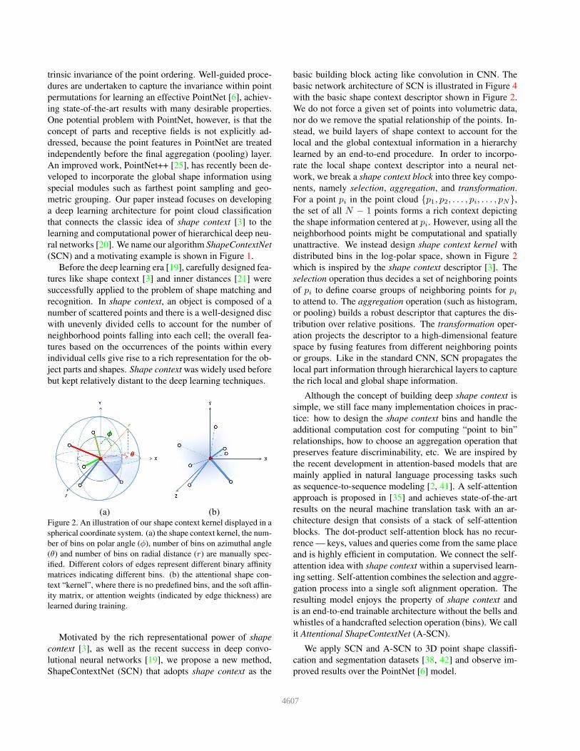
(a) (b)Figure 2. An illustration of our shape context kernel displayed in a

spherical coordinate system. (a) the shape context kernel, the num-

ber of bins on polar angle (φ), number of bins on azimuthal angle

(θ) and number of bins on radial distance (r) are manually spec-

ified. Different colors of edges represent different binary affinity

matrices indicating different bins. (b) the attentional shape con-

text “kernel”, where there is no predefined bins, and the soft affin-

ity matrix, or attention weights (indicated by edge thickness) are

learned during training.

Motivated by the rich representational power of shape

context [3], as well as the recent success in deep convo-

lutional neural networks [19], we propose a new method,

ShapeContextNet (SCN) that adopts shape context as the

basic building block acting like convolution in CNN. The

basic network architecture of SCN is illustrated in Figure 4

with the basic shape context descriptor shown in Figure 2.

We do not force a given set of points into volumetric data,

nor do we remove the spatial relationship of the points. In-

stead, we build layers of shape context to account for the

local and the global contextual information in a hierarchy

learned by an end-to-end procedure. In order to incorpo-

rate the local shape context descriptor into a neural net-

work, we break a shape context block into three key compo-

nents, namely selection, aggregation, and transformation.

For a point pi in the point cloud {p1, p2, . . . , pi, . . . , pN},

the set of all N − 1 points forms a rich context depicting

the shape information centered at pi. However, using all the

neighborhood points might be computational and spatially

unattractive. We instead design shape context kernel with

distributed bins in the log-polar space, shown in Figure 2

which is inspired by the shape context descriptor [3]. The

selection operation thus decides a set of neighboring points

of pi to define coarse groups of neighboring points for pito attend to. The aggregation operation (such as histogram,

or pooling) builds a robust descriptor that captures the dis-

tribution over relative positions. The transformation oper-

ation projects the descriptor to a high-dimensional feature

space by fusing features from different neighboring points

or groups. Like in the standard CNN, SCN propagates the

local part information through hierarchical layers to capture

the rich local and global shape information.

Although the concept of building deep shape context is

simple, we still face many implementation choices in prac-

tice: how to design the shape context bins and handle the

additional computation cost for computing “point to bin”

relationships, how to choose an aggregation operation that

preserves feature discriminability, etc. We are inspired by

the recent development in attention-based models that are

mainly applied in natural language processing tasks such

as sequence-to-sequence modeling [2, 41]. A self-attention

approach is proposed in [35] and achieves state-of-the-art

results on the neural machine translation task with an ar-

chitecture design that consists of a stack of self-attention

blocks. The dot-product self-attention block has no recur-

rence — keys, values and queries come from the same place

and is highly efficient in computation. We connect the self-

attention idea with shape context within a supervised learn-

ing setting. Self-attention combines the selection and aggre-

gation process into a single soft alignment operation. The

resulting model enjoys the property of shape context and

is an end-to-end trainable architecture without the bells and

whistles of a handcrafted selection operation (bins). We call

it Attentional ShapeContextNet (A-SCN).

We apply SCN and A-SCN to 3D point shape classifi-

cation and segmentation datasets [38, 42] and observe im-

proved results over the PointNet [6] model.

4607

2. Method

2.1. Revisiting the Shape Context Descriptor

We first briefly describe the classic shape context de-

scriptor, which was introduced in a seminal work [3] for

2D shape matching and recognition. One main contribution

in [3] is the design of the shape context descriptor with spa-

tially inhomogeneous cells. The neighborhood information

for every point in a set is captured by counting the number

of neighboring points falling inside each cell. The shape de-

scriptor for each point is thus a feature vector (histogram) of

the same dimension as the number of the cells with each fea-

ture dimension depicting the number of points (normalized)

within each cell. The shape context descriptor encodes the

rich contextual shape information using a high-dimensional

vector (histogram) which is particularly suited for matching

and recognition objects in the form of scattered points. For

each point pi in a give point set, shape context computes a

coarse histogram hi of the relative coordinates of the neigh-

boring point,

hi(l) = #{pj 6= pi : (pj − pi) ∈ bin(l)}.

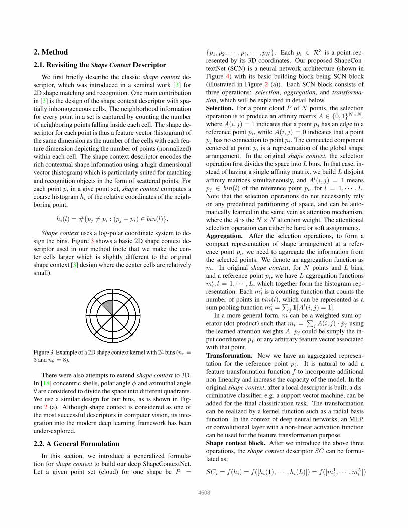
Shape context uses a log-polar coordinate system to de-

sign the bins. Figure 3 shows a basic 2D shape context de-

scriptor used in our method (note that we make the cen-

ter cells larger which is slightly different to the original

shape context [3] design where the center cells are relatively

small).

Figure 3. Example of a 2D shape context kernel with 24 bins (nr =

3 and nθ = 8).

There were also attempts to extend shape context to 3D.

In [18] concentric shells, polar angle φ and azimuthal angle

θ are considered to divide the space into different quadrants.

We use a similar design for our bins, as is shown in Fig-

ure 2 (a). Although shape context is considered as one of

the most successful descriptors in computer vision, its inte-

gration into the modern deep learning framework has been

under-explored.

2.2. A General Formulation

In this section, we introduce a generalized formula-

tion for shape context to build our deep ShapeContextNet.

Let a given point set (cloud) for one shape be P =

{p1, p2, · · · , pi, · · · , pN}. Each pi ∈ R3 is a point rep-

resented by its 3D coordinates. Our proposed ShapeCon-

textNet (SCN) is a neural network architecture (shown in

Figure 4) with its basic building block being SCN block

(illustrated in Figure 2 (a)). Each SCN block consists of

three operations: selection, aggregation, and transforma-

tion, which will be explained in detail below.

Selection. For a point cloud P of N points, the selection

operation is to produce an affinity matrix A ∈ {0, 1}N×N ,

where A(i, j) = 1 indicates that a point pj has an edge to a

reference point pi, while A(i, j) = 0 indicates that a point

pj has no connection to point pi. The connected component

centered at point pi is a representation of the global shape

arrangement. In the original shape context, the selection

operation first divides the space into L bins. In that case, in-

stead of having a single affinity matrix, we build L disjoint

affinity matrices simultaneously, and Al(i, j) = 1 means

pj ∈ bin(l) of the reference point pi, for l = 1, · · · , L.

Note that the selection operations do not necessarily rely

on any predefined partitioning of space, and can be auto-

matically learned in the same vein as attention mechanism,

where the A is the N ×N attention weight. The attentional

selection operation can either be hard or soft assignments.

Aggregation. After the selection operations, to form a

compact representation of shape arrangement at a refer-

ence point pi, we need to aggregate the information from

the selected points. We denote an aggregation function as

m. In original shape context, for N points and L bins,

and a reference point pi, we have L aggregation functions

mli, l = 1, · · · , L, which together form the histogram rep-

resentation. Each mli is a counting function that counts the

number of points in bin(l), which can be represented as a

sum pooling function mli =

∑

j 1[Al(i, j) = 1].

In a more general form, m can be a weighted sum op-

erator (dot product) such that mi =∑

j A(i, j) · pj using

the learned attention weights A. pj could be simply the in-

put coordinates pj , or any arbitrary feature vector associated

with that point.

Transformation. Now we have an aggregated represen-

tation for the reference point pi. It is natural to add a

feature transformation function f to incorporate additional

non-linearity and increase the capacity of the model. In the

original shape context, after a local descriptor is built, a dis-

criminative classifier, e.g. a support vector machine, can be

added for the final classification task. The transformation

can be realized by a kernel function such as a radial basis

function. In the context of deep neural networks, an MLP,

or convolutional layer with a non-linear activation function

can be used for the feature transformation purpose.

Shape context block. After we introduce the above three

operations, the shape context descriptor SC can be formu-

lated as,

SCi = f(hi) = f([hi(1), · · · , hi(L)]) = f([m1

i , · · · ,mLi ])

4608

Figure 4. ShapeContextNet (SCN) and Attentional ShapeContextNet (A-SCN) architectures. The classification network has 5

ShapeContext blocks; each block takes N point feature vectors as input, and applies the selection, aggregation and transformation opera-

tions sequentially. The ShapeContext blocks can be implemented by hand-designed shape context kernels (SCN block), or a self-attention

mechanism learned from data (A-SCN block). See text in Section 2 for details.

where mli =

∑

j 1[Al(i, j) = 1]. Note that every com-

ponents in this formulation can be implemented by a back-

propagatable neural network module, and thus, similar to a

convolutional layer, SC is a compositional block that can

be used to build a shape context network,

SCNet = SCi(SCi(SCi(· · · )))

2.3. ShapeContextNet

Shape context kernel. Similar to [18], we use concentric

shells to design the shape context kernel. The kernel is ad-

justable with three parameters: polar angle φ, azimuthal an-

gle θ and radial distance r (Figure 2 (a)). In our setting, φ

and θ are evenly divided into different sectors, while for r,

a logarithmic parametrization of the shell radii is used. We

also set a maximum radius of the sphere max R, which de-

fines the receptive field size for a single shape context ker-

nel. Thus the design of the shape context kernel is paramer-

ized by the maximum radius (max R), the number of bins

for radius r (nr), angles θ (nθ) and angles φ (nφ). The com-

bined number of bins for a shape context kernel is equal to

nr × nθ × nφ.

Selection. With the L bins induced by a shape context ker-

nel, the selection operation builds L disjoint affinity matri-

ces A1, · · · , AL, where each matrix is corresponding to a

specific bin. We generate the affinity matrices online during

training and share them across different layers.

Aggregation. Following original shape context, the aggre-

gation operation is simply a sum-pooling layer that aggre-

gates points (associated with D-dimensional feature vec-

tors) within each bin. Note that the sum-pooling layer

can be implemented by L parallel matrix multiplications,

as AL is binary. The aggregation operation results in L

sets of pooled features, thus the output is a tensor of shape

N × L×D.

Transformation. Finally the transformation operation is

realized by a convolutional layer with a [L, 1] kernel that

fuses L sets of feature points and projects them to (higher

dimensional) output feature vectors of Dout. A ShapeCon-

text block consists of above operations and our ShapeCon-

textNet is a stack of ShapeContext blocks with increas-

ing output dimensions of Dout. We follow the over-

all network configuration of PointNet and use Dout =(64, 64, 64, 128, 1024) as the output dimensions for each

ShapeContext block.

Limitations. While being conceptually simple and en-

4609

joying good properties of classic shape context descrip-

tors such as translation-invariance, handcrafting shape con-

text kernels are not straight-forward and hard to general-

ize across different point cloud datasets which usually have

varying size and density. This motivates us to propose the

following attention-based model.

2.4. Attentional ShapeContextNet

We now introduce a different approach inspired by

research in natural language processing (sequence-to-

sequence) tasks. Traditional sequence-to-sequence models

usually adopt recurrent neural networks (e.g. LSTM[15]),

external memory or temporal convolutions to capture the

context information. The dot-product self-attention pro-

posed in [35] is a model that handles long path-length

contextual modeling by a light-weight gating mechanism,

where the attention weight matrix is generated using a

simple dot-product. It is worth-noting that self-attention

is also invariant to the input ordering. Unlike traditional

attention-based sequence-to-sequence models, in a self-

attention block, query vector Q ∈ RDQ , key vector K ∈RDK (usually DQ = DK) and value vector V ∈ RDV are

learned from the same input. In a supervised classification

setting, one can think Q, K and V are just three feature

vectors learned by three independent MLP layers. Atten-

tion weights are computed by a dot product of Q and K,

and then multiplied with V to obtain the transformed repre-

sentation.

Figure 2 shows the similarities and differences between

manually specified shape context kernels and the automat-

ically learnable self-attention mechanism: They all aim to

capture the distribution over relative positions; they are uni-

fied under the same formulation in Section 2.2; the selection

operation in self-attention does not rely on hand-designed

bin partitioning as it can be learned from data; self-attention

has better modeling capability by adopting a weighted sum

aggregation function, in contrast to using a simple sum-

pooling function.

Selection and Aggregation. We consider computing self-

attention on the whole point cloud P of size N . The se-

lection operation produces a soft affinity matrix, which is

the self-attention weight matrix A of size N × N , the ag-

gregation operation is transforming the value vector V with

weight matrix A by a dot product,

Attention(Q, V,K) = Softmax(QKT

√

DQ

) · V (1)

Transformation. MLPs with ReLU activation function can

be added as a feature transformation operation after each

self-attention operation (Equation 1). To further improve

the model expressiveness, we add a simple feature gating

layer to the MLP, similar to [8, 24].

Figure 5. Ablation analysis on the number of ShapeContext

blocks. The error rates obtained by increasing the number of

ShapeContext blocks. Metric is overall accuracy on 2D MNIST

test set (N = 256). The bin configuration is: max R = 0.5, nr = 3,

nθ = 12.

Model N Error rate (%)

PointNet[6] 256 0.78

PointNet++[25] 512 0.51

shape context local 256 1.18

ShapeContextNet 256 0.60

Table 1. 2D point cloud classification results on the MNIST

dataset. ShapeContextNet achieves better performance than Point-

Net showing the effectiveness of contextual information; the shape

context local model consists of only one shape context block.

3. Experimental Results

3.1. ShapeContextNets: 2D case

We first showcase the effectiveness of deep ShapeCon-

textNet which has a stack of shape context blocks.

2D point set is generated for MNIST dataset following

the same protocol as used in PointNet[6], where 256 points

are sampled for each digit. We use a shape context kernel

with max R = 0.5, nr = 3 and nθ = 12, thus 36 bins in

total.

Table 1 shows that a simple 5-layer SCN achieves better

performance than PointNet, showing that using the distri-

bution over relative positions as a context feature is indeed

helpful for the shape recognition task. The performance

of SCN is also competitive to the recent PointNet++[25]

model which uses 512 points as input. shape context local is

a model that consists of only one shape context block, which

resembles the “feature extraction and classifier learning”

pipeline in traditional computer vision. To better under-

stand the importance of hierarchical learning in ShapeCon-

textNet, in Figure 5, we vary the number of shape context

blocks from 0 to 5 in the network (Figure 4), where the 5-

layer model is our ShapeContextNet, the 1-layer model is

the shape context local model, and 0 means no shape con-

4610

text block. We observe that as the number of shape context

blocks increases, the error rate decreases.

3.2. ShapeContextNets: 3D case

We evaluate the 3D shape classification performance of

SCN on the ModelNet40[38] dataset, with point cloud data

from 12,311 CAD models in 40 categories. We use 9,843

for training and 2,468 for testing. Following [6], 1,024

points are sampled for each training/testing instance. Ta-

ble 2 summarizes the impact of different shape context ker-

nel design choices parametrized by max R, nr, nθ and nφ.

max No. of No. of No. of accuracy accuracy

R r bins θ bins φ bins avg. class overall

PointNet vanilla[6] - - - - - 87.1

PointNet[6] - - - - 86.2 89.2

PointNet++[25] - - - - - 90.7

(A) 0.25 3 3 3 86.2 89.3

(B) 1 84.8 88.6

(C) 0.5 2 86.7 89.6

(D) 4 86.5 89.6

(E) 3 2 81.4 84.8

(F) 4 82.2 84.2

(G) 3 2 85.5 88.9

(H) 4 87.5 89.7

SCN (I) 0.5 3 3 3 87.6 90.0

Table 2. Ablation analysis on shape context kernel design in

ShapeContextNet. We evaluate SCN models with different ker-

nel configurations (model (A)-(I)). max R is the maximum lo-

cal radius for the sphere shape context kernel at each reference

point. nr , nθ and nφ are the number of different shell and angle

bins. Unlisted values are identical to those of the preceding model.

We report averaged and overall accuracy on ModelNet40 test set

(N=1024).

We obtain the best results with max R = 0.5. Note that

the coordinates of point cloud in ModelNet40 are normal-

ized to [−1, 1]. This means the receptive field of a single

shape context kernel covers around a quarter of the entire

point cloud. With the same radius bin configuration, the

test accuracy peaks when nr = nθ = nφ = 3. Empirically,

the number of r bins has the least impact on the test accu-

racy, whereas the number of θ bins appears to be crucial for

the performance. With minimal change in architecture to a

vanilla PointNet (by replacing the MLP layers to carefully

designed shape context kernels), ShapeContextNet (model

(I)) achieves better or competitive results compared to full

PointNet model (with additional input/feature transforma-

tion layers), and the recent PointNet++ model (with special

sampling/grouping modules).

3.3. Attentional ShapeContextNet

ModelNet40 Shape Classification. The architecture of

Attentional ShapeContextNet (A-SCN) follows the gen-

eral design of ShapeContextNet (SCN). In contrast to

using hand-crafted shape context kernels, we adopt the

self-attention module as the shape context block in the

network (Figure 4). Q, K and V feature vectors are

ReLU BN residual Num of accuracy accuracy

A-SCN Q=K? Q/K/V Q/K/V connect. heads avg. class overall

(A) ✓ ✓/✓/✓ ✓/✓/✓ ✓ 1 85.7 89.0

(B) ✗ 28.2 36.7

(C) ✗ ✓ 85.7 89.1

(D) ✗/✗/✗ 86.1 89.2

(E) ✗/✗/✓ 87.4 89.8

(F) 2 86.3 89.2

(G) 4 87.2 89.8

Table 3. Ablation analysis on the Attentional ShapeContextNet

architecture. We evaluate the Attentional ShapeContextNet

model on ModelNet40 dataset with different hyperparameter set-

tings (model (A)-(G)). We report class-averaged and overall ac-

curacy on test set. Unlisted values are identical to those of the

preceding model. Q, K and V here represent the feature vectors

learned in an A-SCN block (Figure 4).

learned from the input using three MLPs. We use

DK = DQ = (32, 32, 32, 32, 64) and DV = Dout =(64, 64, 64, 128, 1024) for each block. Attention weight

matrix of shape N × N is computed according to Equa-

tion 1. Table 3 summarizes the performance of A-SCN with

different hyperparameters. The choices of different hyper-

parameters are generally aligned with those in [35] on the

machine translation task. For example, the residual connec-

tion is necessary in order to learn a good model, and learn-

ing Q and K vectors independently is better than weight-

sharing. Note that similar to SCN where L affinity matrices

are used, we can also learn multiple attention weights in

parallel for A-SCN. This is called multi-head attention in

[35]. However, empirically we find that using multi-head

attention does not yield better performance comparing to

the one-head model, and introduces additional computation

overhead. Therefore, in this paper A-SCN refers to our one-

head model (model (E)). A-SCN is able to achieve 89.8%

overall accuracy, which is on par with SCN, but with a sim-

pler design and fewer critical hyper-parameter to set.

In Figure 6 we show surprisingly diverse and semanti-

cally meaningful behavior of the learned attention weights.

For a reference point, it oftentimes attends to areas far away

to itself. The selected areas are usually descriptive and dis-

criminative parts of a model, e.g. back or legs of a chair.

Figure 7 visualizes how shape information is propagated

and condensed into a compact representation in a multi-

level neural network. For a fixed reference points, attention

becomes increasingly sparse, and focuses on smaller areas

when the level gets higher.

ShapeNet Part Segmentation. Part segmentation is a

challenging task in 3D object recognition domain. Given a

set of points of a 3D shape model (e.g. a plane), the part

segmentation task is to label each point in the set as one

of the model’s part (e.g. engine, body, wing and tail). We

follow the experimental setup in [6], and defines the task as

a point-wise classification problem.

Our model (A-SCN) is trained and evaluated on

4611

mean aero bag cap car chair ear guitar knife lamp laptop motor mug pistol rocket skate table

phone board

# shapes 2690 76 55 898 3758 69 787 392 1547 451 202 184 283 66 152 5271

Wu [37] - 63.2 - - - 73.5 - - - 74.4 - - - - - - 74.8

Yi [42] 81.4 81.0 78.4 77.7 75.7 87.6 61.9 92.0 85.4 82.5 95.7 70.6 91.9 85.9 53.1 69.8 75.3

3DCNN[6] 79.4 75.1 72.8 73.3 70.0 87.2 63.5 88.4 79.6 74.4 93.9 58.7 91.8 76.4 51.2 65.3 77.1

PointNet++[25] 85.1 82.4 79.0 87.7 77.3 90.8 71.8 91.0 85.9 83.7 95.3 71.6 94.1 81.3 58.7 76.4 82.6

PointNet[6] 83.7 83.4 78.7 82.5 74.9 89.6 73.0 91.5 85.9 80.8 95.3 65.2 93.0 81.2 57.9 72.8 80.6

A-SCN (ours) 84.6 83.8 80.8 83.5 79.3 90.5 69.8 91.7 86.5 82.9 96.0 69.2 93.8 82.5 62.9 74.4 80.8

Table 4. Segmentation results on ShapeNet part dataset. We compared the results with Wu [37], Yi [42], 3DCNN from [6], PointNet [6]

and recent PointNet++[25] which uses additional normal direction features. The results are evaluated with mean IoUs(%) metric on points.

Our A-SCN model achieves competitive performance for point cloud part segmentation.

Figure 6. Attention weights learned by A-SCN on three shape models: a plane, a chair and a toilet. First column in each row shows

the original point cloud. The other columns visualize learned weights for one randomly sampled reference point. Higher value indicates

stronger connection to the reference point. Attention weights learned by A-SCN are diverse, sparse, and semantically meaningful and a

reference point learns to attend to discriminative parts of a model.

Block 1 Block 2 Block 3 Block 4

Figure 7. Attention weights learned on different levels. In A-

SCN, shape information is propagated and condensed into a com-

pact representation through a multi-level network structure. From

left to right are attention weights, for a fixed reference point,

learned in the first, second, third and fourth attentional shape con-

text block. Attention becomes increasingly sparse, and focuses on

smaller areas with compact representations.

ShapeNet part dataset following the data split from [5].

ShapeNet part dataset [42] consists of 16,881 object from

16 object categories, where each object category is labeled

with 2-5 parts. During training, we randomly sample 1024

points from the 3D point cloud of each object and use

cross-entropy as our loss function. We also followed the

settings from [42], which assume the object category label

is known. During testing, we test the model on all the

points from each object and evaluated using point mean

intersection over union (mIoU), averaged across all part

classes, similar to [6]. Our A-SCN model outperforms

PointNet in terms of mean IoUs over most of categories,

and is on par with the recent PointNet++ model which aug-

ment the input points with additional normal information.

Full results for part segmentation are listed in Table 4.

4612

Input Scene Ground Truth PointNet A-SCN

Figure 8. Visualization of semantic segmentation results by A-SCN. From left to right: original input scenes; ground truth point cloud

segmentation; PointNet[6] segmentation results and Attentional ShapeContextNet (A-SCN) segmentation results. Color mappings are red:

chairs, purple: tables , orange: sofa, gray: board, green: bookcase, blue: floors, violet: windows, yellow: beam, magenta: column, khaki:

doors and black: clutters.

S3DIS Semantic Segmentation. Stanford 3D indoor

scene dataset[1] includes 6 large scale areas that in total

have 271 indoor scenes. Each point in the scene point cloud

is associated with one label in 13 categories. We follow

[6] for data pre-processing, dividing the scene point cloud

into small blocks. We also use the same k-fold strategy for

training and testing. We randomly sample 2,048 points from

each block for training and use all the points for testing. For

each point, we use the XYZ coordinates, RGB value and the

normalized coordinates as its input vector.

mean IoU(%) overall accuracy (%)

PointNet [6] 47.71 78.62

A-SCN (ours) 52.72 81.59

Table 5. Results on scene semantic segmentation. Mean

IoU(%) on and point-wise accuracy are reported. Our Attentional

ShapeContextNet model outperforms PointNet in both metrics.

The evaluation results of our method are in Figure 5.

By taking into account the global shape context in a hier-

archical learning way, our A-SCN model achieves 52.72%

in mean IoU and 81.59% in point-wise accuracy, improv-

ing the results by PointNet in both metrics. Some of our

segmentation results are visualized in Figure 8.

4. Conclusion

To tackle the recognition problem for 3D/2D point

clouds, we develop a new neural network based algorithm

by adopting the concept of shape context to build our basic

building block, shape context kernel. The resulting model,

named as ShapeContextNet (SCN), consists of hierarchical

modules that are able to represent the intrinsic property of

object points by capturing and propagating both the local

part and the global shape information. In addition, we pro-

pose an Attentional ShapeContextNet (A-SCN) model to

automate the process for contextual region selection, fea-

ture aggregation, and feature transformation. We validated

the effectiveness of our model on a number of benchmark

datasets and observed encouraging results.

Acknowledgment

This work is funded by NSF IIS-1618477 and NSF IIS-

1717431. S. Xie is supported by Google. The authors would like

to thank Justin Lazarow for insightful discussions, Hao Su and

Charles R. Qi for helping with the MNIST experiment setup.

4613

References

[1] I. Armeni, O. Sener, A. R. Zamir, H. Jiang, I. Brilakis,

M. Fischer, and S. Savarese. 3d semantic parsing of large-

scale indoor spaces. In CVPR, 2016. 8

[2] D. Bahdanau, K. Cho, and Y. Bengio. Neural machine trans-

lation by jointly learning to align and translate. In ICLR,

2015. 2

[3] S. Belongie, J. Malik, and J. Puzicha. Shape matching and

object recognition using shape contexts. TPAMI, 24(4):509–

522, 2002. 2, 3

[4] J. Carreira and A. Zisserman. Quo vadis, action recognition?

a new model and the kinetics dataset. In CVPR, 2017. 1

[5] A. X. Chang, T. Funkhouser, L. Guibas, P. Hanrahan,

Q. Huang, Z. Li, S. Savarese, M. Savva, S. Song, H. Su,

et al. Shapenet: An information-rich 3d model repository.

arXiv preprint arXiv:1512.03012, 2015. 1, 7

[6] R. Q. Charles, H. Su, M. Kaichun, and L. J. Guibas. Pointnet:

Deep learning on point sets for 3d classification and segmen-

tation. In CVPR, 2017. 1, 2, 5, 6, 7, 8

[7] D.-Y. Chen, X.-P. Tian, Y.-T. Shen, and M. Ouhyoung. On

visual similarity based 3d model retrieval. In Computer

graphics forum, 2003. 1

[8] Y. N. Dauphin, A. Fan, M. Auli, and D. Grangier. Language

modeling with gated convolutional networks. In ICML,

2017. 5

[9] J. Deng, W. Dong, R. Socher, L.-J. Li, K. Li, and L. Fei-Fei.

ImageNet: A Large-Scale Hierarchical Image Database. In

CVPR, 2009. 1

[10] Q. Dou, L. Yu, H. Chen, Y. Jin, X. Yang, J. Qin, and P.-A.

Heng. 3d deeply supervised network for automated segmen-

tation of volumetric medical images. Medical Image Analy-

sis, 2017. 1

[11] R. Girshick, J. Donahue, T. Darrell, and J. Malik. Rich Fea-

ture Hierarchies for Accurate Object Detection and Semantic

Segmentation. In CVPR, 2014. 1

[12] K. Guo, D. Zou, and X. Chen. 3d mesh labeling via deep con-

volutional neural networks. ACM Transactions on Graphics

(TOG), 35(1):3, 2015. 1

[13] K. He, G. Gkioxari, P. Dollar, and R. Girshick. Mask r-cnn.

In ICCV, 2017. 1

[14] K. He, X. Zhang, S. Ren, and J. Sun. Deep Residual Learning

for Image Recognition. In CVPR, 2016. 1

[15] S. Hochreiter and J. Schmidhuber. Long short-term memory.

Neural computation, 9(8):1735–1780, 1997. 5

[16] G. Huang, Z. Liu, L. van der Maaten, and K. Q. Weinberger.

Densely connected convolutional networks. In CVPR, 2017.

1

[17] S. Ji, W. Xu, M. Yang, and K. Yu. 3d convolutional neural

networks for human action recognition. TPAMI, 35(1):221–

231, 2013. 1

[18] M. Kortgen, G. Park, M. Novotni, and R. Klein. 3d shape

matching with 3d shape contexts. In In the 7th Central Eu-

ropean Seminar on Computer Graphics, 2003. 3, 4

[19] A. Krizhevsky, I. Sutskever, and G. E. Hinton. Imagenet

classification with deep convolutional neural networks. In

NIPS, 2012. 1, 2

[20] Y. LeCun, B. Boser, J. S. Denker, D. Henderson, R. E.

Howard, W. Hubbard, and L. D. Jackel. Backpropagation

applied to handwritten zip code recognition. Neural compu-

tation, 1(4):541–551, 1989. 1, 2

[21] H. Ling and D. W. Jacobs. Shape classification using the

inner-distance. TPAMI, 29(2):286–299, 2007. 2

[22] J. Long, E. Shelhamer, and T. Darrell. Fully convolutional

networks for semantic segmentation. In CVPR, 2015. 1

[23] A. Payan and G. Montana. Predicting alzheimer’s disease: a

neuroimaging study with 3d convolutional neural networks.

arXiv preprint arXiv:1502.02506, 2015. 1

[24] E. Perez, F. Strub, H. de Vries, V. Dumoulin, and

A. Courville. Film: Visual reasoning with a general con-

ditioning layer. In AAAI, 2018. 5

[25] C. R. Qi, L. Yi, H. Su, and L. J. Guibas. Pointnet++: Deep

hierarchical feature learning on point sets in a metric space.

In NIPS, 2017. 2, 5, 6, 7

[26] S. Ren, K. He, R. Girshick, and J. Sun. Faster r-cnn: Towards

real-time object detection with region proposal networks. In

NIPS, 2015. 1

[27] R. B. Rusu, N. Blodow, and M. Beetz. Fast point feature

histograms (fpfh) for 3d registration. In IEEE Robotics and

Automation, 2009. 1

[28] M. Savva, F. Yu, H. Su, M. Aono, B. Chen, D. Cohen-Or,

W. Deng, H. Su, S. Bai, X. Bai, et al. Shrec16 track: large-

scale 3d shape retrieval from shapenet core55. In Eurograph-

ics Workshop on 3D Object Retrieval, 2016. 1

[29] K. Simonyan and A. Zisserman. Very deep convolutional

networks for large-scale image recognition. In ICLR, 2015.

1

[30] H. Su, S. Maji, E. Kalogerakis, and E. Learned-Miller. Multi-

view convolutional neural networks for 3d shape recognition.

In ICCV, 2015. 1

[31] C. Szegedy, W. Liu, Y. Jia, P. Sermanet, S. Reed,

D. Anguelov, D. Erhan, V. Vanhoucke, and A. Rabinovich.

Going deeper with convolutions. In CVPR, 2015. 1

[32] C. Szegedy, V. Vanhoucke, S. Ioffe, J. Shlens, and Z. Wojna.

Rethinking the inception architecture for computer vision. In

CVPR, 2016. 1

[33] D. Tran, L. Bourdev, R. Fergus, L. Torresani, and M. Paluri.

Learning spatiotemporal features with 3d convolutional net-

works. In ICCV, 2015. 1

[34] D. Tran, H. Wang, L. Torresani, J. Ray, Y. LeCun, and

M. Paluri. A closer look at spatiotemporal convolutions for

action recognition. arXiv preprint arXiv:1711.11248, 2017.

1

[35] A. Vaswani, N. Shazeer, N. Parmar, J. Uszkoreit, L. Jones,

A. N. Gomez, Ł. Kaiser, and I. Polosukhin. Attention is all

you need. In NIPS, 2017. 2, 5, 6

[36] D. Z. Wang and I. Posner. Voting for voting in online point

cloud object detection. In Robotics: Science and Systems,

2015. 1

[37] Z. Wu, R. Shou, Y. Wang, and X. Liu. Interactive shape co-

segmentation via label propagation. Computers & Graphics,

38:248–254, 2014. 7

[38] Z. Wu, S. Song, A. Khosla, F. Yu, L. Zhang, X. Tang, and

J. Xiao. 3d shapenets: A deep representation for volumetric

shapes. In CVPR, 2015. 1, 2, 6

4614

[39] S. Xie, R. Girshick, P. Dollar, Z. Tu, and K. He. Aggregated

residual transformations for deep neural networks. In CVPR,

2017. 1

[40] S. Xie, C. Sun, J. Huang, Z. Tu, and K. Murphy. Rethink-

ing spatiotemporal feature learning for video understanding.

arXiv preprint arXiv:1712.04851, 2017. 1

[41] K. Xu, J. Ba, R. Kiros, K. Cho, A. Courville, R. Salakhudi-

nov, R. Zemel, and Y. Bengio. Show, attend and tell: Neural

image caption generation with visual attention. In ICML,

2015. 2

[42] L. Yi, V. G. Kim, D. Ceylan, I. Shen, M. Yan, H. Su, A. Lu,

Q. Huang, A. Sheffer, L. Guibas, et al. A scalable active

framework for region annotation in 3d shape collections.

ACM Transactions on Graphics (TOG), 35(6):210, 2016. 1,

2, 7

[43] B. Zoph and Q. V. Le. Neural architecture search with rein-

forcement learning. In ICLR, 2017. 1

4615