attia, john okyere. “ transient analysis.” electronics and circuit analysis...

Attia, John Okyere. “Transient Analysis.”Electronics and Circuit Analysis using MATLAB.Ed. John Okyere AttiaBoca Raton: CRC Press LLC, 1999

© 1999 by CRC PRESS LLC

CHAPTER FIVE

TRANSIENT ANALYSIS

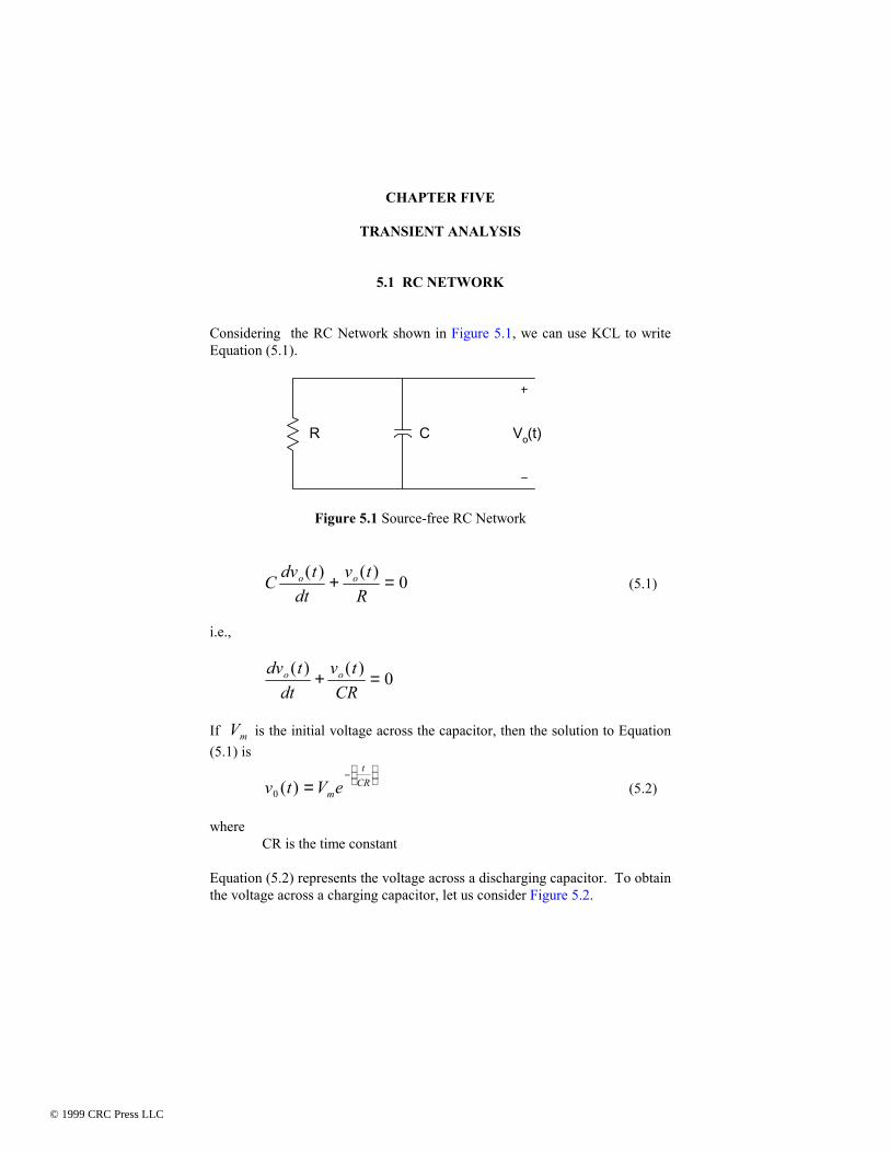
5.1 RC NETWORK Considering the RC Network shown in Figure 5.1, we can use KCL to write Equation (5.1).

R C Vo(t)

Figure 5.1 Source-free RC Network

C dv tdt

v tR

o o( ) ( )+ = 0 (5.1)

i.e.,

dv t

dtv tCR

o o( ) ( )+ = 0

If Vm is the initial voltage across the capacitor, then the solution to Equation (5.1) is

v t V em

tCR

0 ( ) =−

(5.2)

where CR is the time constant Equation (5.2) represents the voltage across a discharging capacitor. To obtain the voltage across a charging capacitor, let us consider Figure 5.2.

© 1999 CRC Press LLC


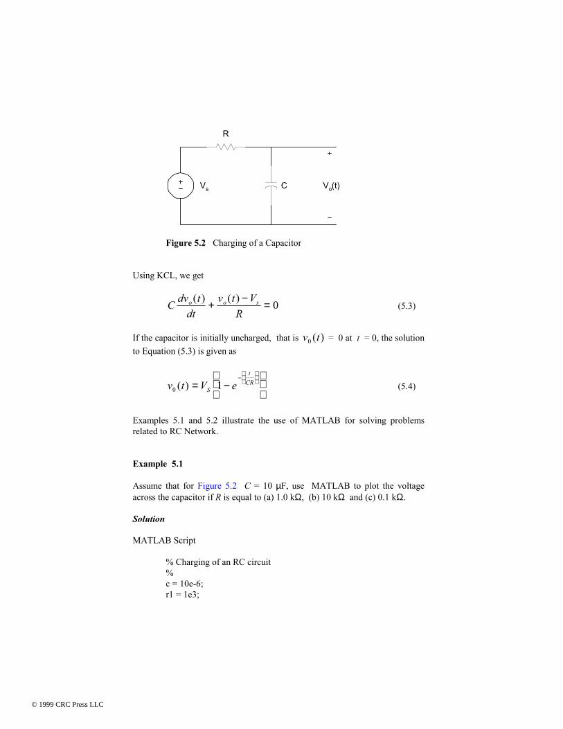
Vo(t)

R

CVs

Figure 5.2 Charging of a Capacitor Using KCL, we get

C dv tdt

v t VR

o o s( ) ( )+ − = 0 (5.3)

If the capacitor is initially uncharged, that is v t0 ( ) = 0 at t = 0, the solution to Equation (5.3) is given as

v t V eS

tCR

0 1( ) = −

−

(5.4)

Examples 5.1 and 5.2 illustrate the use of MATLAB for solving problems related to RC Network. Example 5.1 Assume that for Figure 5.2 C = 10 µF, use MATLAB to plot the voltage across the capacitor if R is equal to (a) 1.0 kΩ, (b) 10 kΩ and (c) 0.1 kΩ. Solution MATLAB Script

% Charging of an RC circuit % c = 10e-6; r1 = 1e3;



tau1 = c*r1; t = 0:0.002:0.05; v1 = 10*(1-exp(-t/tau1)); r2 = 10e3; tau2 = c*r2; v2 = 10*(1-exp(-t/tau2)); r3 = .1e3; tau3 = c*r3; v3 = 10*(1-exp(-t/tau3)); plot(t,v1,'+',t,v2,'o', t,v3,'*') axis([0 0.06 0 12]) title('Charging of a capacitor with three time constants') xlabel('Time, s') ylabel('Voltage across capacitor') text(0.03, 5.0, '+ for R = 1 Kilohms') text(0.03, 6.0, 'o for R = 10 Kilohms') text(0.03, 7.0, '* for R = 0.1 Kilohms')

Figure 5.3 shows the charging curves.

Figure 5.3 Charging of Capacitor



From Figure 5.3, it can be seen that as the time constant is small, it takes a short time for the capacitor to charge up. Example 5.2 For Figure 5.2, the input voltage is a rectangular pulse with an amplitude of 5V and a width of 0.5s. If C = 10 µF, plot the output voltage, v t0 ( ) , for resistance R equal to (a) 1000 Ω, and (b) 10,000 Ω. The plots should start from zero seconds and end at 1.5 seconds. Solution MATLAB Script

% The problem will be solved using a function program rceval function [v, t] = rceval(r, c) % rceval is a function program for calculating % the output voltage given the values of % resistance and capacitance. % usage [v, t] = rceval(r, c) % r is the resistance value(ohms) % c is the capacitance value(Farads) % v is the output voltage % t is the time corresponding to voltage v tau = r*c; for i=1:50 t(i) = i/100; v(i) = 5*(1-exp(-t(i)/tau)); end vmax = v(50); for i = 51:100 t(i) = i/100; v(i) = vmax*exp(-t(i-50)/tau); end end % The problem will be solved using function program % rceval % The output is obtained for the various resistances c = 10.0e-6; r1 = 2500;



[v1,t1] = rceval(r1,c); r2 = 10000; [v2,t2] = rceval(r2,c); % plot the voltages plot(t1,v1,'*w', t2,v2,'+w') axis([0 1 0 6]) title('Response of an RC circuit to pulse input') xlabel('Time, s') ylabel('Voltage, V') text(0.55,5.5,'* is for 2500 Ohms') text(0.55,5.0, '+ is for 10000 Ohms')

Figure 5.4 shows the charging and discharging curves.

Figure 5.4 Charging and Discharging of a Capacitor with Different Time Constants



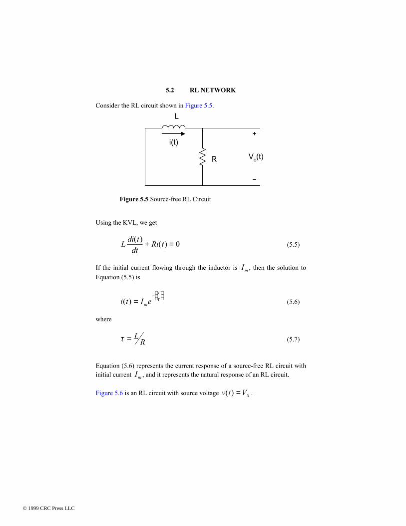
5.2 RL NETWORK Consider the RL circuit shown in Figure 5.5.

L

R Vo(t)

i(t)

Figure 5.5 Source-free RL Circuit Using the KVL, we get

L di tdt

Ri t( ) ( )+ = 0 (5.5)

If the initial current flowing through the inductor is Im , then the solution to Equation (5.5) is

i t I em

t

( ) =−

τ (5.6)

where

τ = LR (5.7)

Equation (5.6) represents the current response of a source-free RL circuit with initial current Im , and it represents the natural response of an RL circuit. Figure 5.6 is an RL circuit with source voltage v t VS( ) = .



VR(t)

L

Ri(t)

V(t)

Figure 5.6 RL Circuit with a Voltage Source Using KVL, we get

Ldi t

dtRi t VS

( )( )+ = (5.8)

If the initial current flowing through the series circuit is zero, the solution of Equation (5.8) is

i tVR

eSRtL( ) = −

−

1 (5.9)

The voltage across the resistor is v t Ri tR ( ) ( )=

= V eS

RtL1−

−

(5.10)

The voltage across the inductor is v t V v tL S R( ) ( )= −

=−

V eS

RtL (5.11)

The following example illustrates the use of MATLAB for solving RL circuit problems.



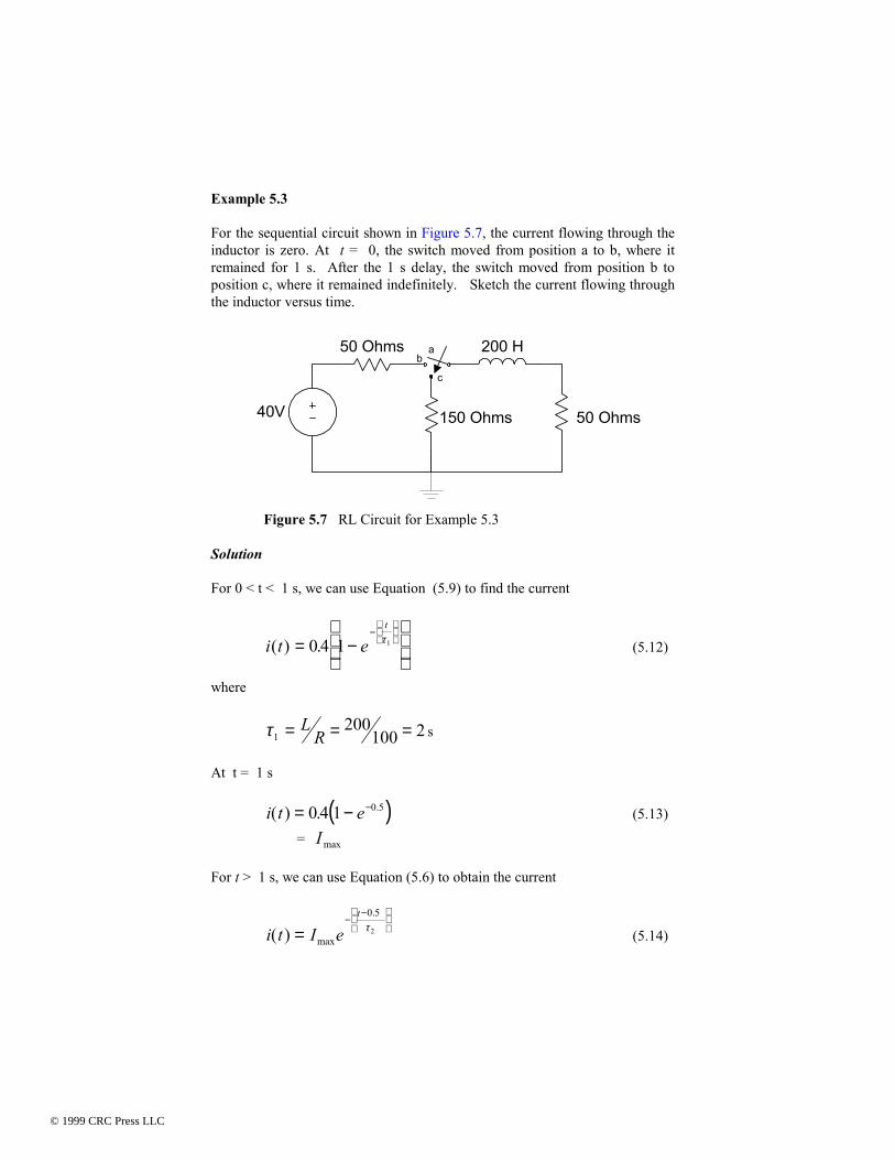
Example 5.3 For the sequential circuit shown in Figure 5.7, the current flowing through the inductor is zero. At t = 0, the switch moved from position a to b, where it remained for 1 s. After the 1 s delay, the switch moved from position b to position c, where it remained indefinitely. Sketch the current flowing through the inductor versus time.

40V

50 Ohms

150 Ohms

200 H

50 Ohms

ab

c

Figure 5.7 RL Circuit for Example 5.3 Solution For 0 < t < 1 s, we can use Equation (5.9) to find the current

i t et

( ) .= −

−

0 4 1 1τ (5.12)

where

τ1200

100 2= = =LR s

At t = 1 s

( )i t e( ) . .= − −0 4 1 0 5 (5.13)

= Imax For t > 1 s, we can use Equation (5.6) to obtain the current

i t I et

( ) max

.

=−

−

0 5

2τ (5.14)



where

τ 22

200200 1= = =L

Req s

The MATLAB program for plotting i t( ) is shown below. MATLAB Script

% Solution to Example 5.3 % tau1 is time constant when switch is at b % tau2 is the time constant when the switch is in position c % tau1 = 200/100; for k=1:20 t(k) = k/20; i(k) = 0.4*(1-exp(-t(k)/tau1)); end imax = i(20); tau2 = 200/200; for k = 21:120 t(k) = k/20; i(k) = imax*exp(-t(k-20)/tau2); end % plot the current plot(t,i,'o') axis([0 6 0 0.18]) title('Current of an RL circuit') xlabel('Time, s') ylabel('Current, A')

Figure 5.8 shows the current i t( ) .



Figure 5.8 Current Flowing through Inductor

5.3 RLC CIRCUIT For the series RLC circuit shown in Figure 5.9, we can use KVL to obtain the Equation (5.15).

Vo(t)

L

RVs(t) = Vs

i(t)

Figure 5.9 Series RLC Circuit



v t Ldi t

dt Ci d Ri tS

t

( )( )

( ) ( )= + +−∞∫

1τ τ (5.15)

Differentiating the above expression, we get

dv t

dtL

d i tdt

Rdi t

dti tC

S ( ) ( ) ( ) ( )= + +

2

2

i.e.,

1 2

2Ldv t

dtd i t

dtRL

di tdt

i tLC

S ( ) ( ) ( ) ( )= + + (5.16)

The homogeneous solution can be found by making v tS ( ) = constant, thus

02

2= + +d i tdt

RL

di tdt

i tLC

( ) ( ) ( ) (5.17)

The characteristic equation is 0 2= + +λ λa b (5.18) where

a RL= and

b LC= 1 The roots of the characteristic equation can be determined. If we assume that the roots are λ α β= , then, the solution to the homogeneous solution is i t A e A eh

t t( ) = +1 21 2α α (5.19)

where



A1 and A2 are constants. If v tS ( ) is a constant, then the forced solution will also be a constant and be given as i t Af ( ) = 3 (5.20) The total solution is given as i t A e A e At t( ) = + +1 2 3

1 2α α (5.21) where

A1 , A2 , and A3 are obtained from initial conditions. Example 5.4 illustrates the use of MATLAB for finding the roots of characteristic equations. The MATLAB function roots, described in Section 6.3.1, is used to obtain the roots of characteristic equations. Example 5.4 For the series RLC circuit shown in Figure 5.9, If L = 10 H, R = 400 Ohms

and C = 100µF, v tS ( ) = 0, i( )0 4= A anddi

dt( )0 15= A/s, find i t( ) .

Solution Since v tS ( ) = 0, we use Equation (5.17) to get

0 40010

10002

2= + +d i tdt

di tdt

i t( ) ( ) ( )

The characteristic equation is 0 40 10002= + +λ λ The MATLAB function roots is used to obtain the roots of the characteristics equation.



MATLAB Script

p = [1 40 1000]; lambda = roots(p) lambda = -20.0000 +24.4949i -20.0000 -24.4949i

Using the roots obtained from MATLAB, i t( ) is given as i t e A t A tt( ) ( cos( . ) sin( . )= +−20

1 224 4949 24 4949 i e A A A( ) ( ( ))0 0 40

1 2 1= + ⇒ =−

[ ][ ]

di tdt

e A t A t

e A t A t

t

t

( )cos( . ) sin( . )

. sin( . ) . cos( . )

= − + +

− +

−

−

20 24 4949 24 4949

24 4949 24 4949 24 4949 24 4949

201 2

201 2

di

dtA A

( ).

024 4949 20 152 1= − =

Since A1 4= , A2 38784= .

[ ]i t e t tt( ) cos( . ) . sin( . )= +−20 4 24 4949 38784 24 4949 Perhaps the simplest way to obtain voltages and currents in an RLC circuit is to use Laplace transform. Table 5.1 shows Laplace transform pairs that are useful for solving RLC circuit problems. From the RLC circuit, we write differential equations by using network analysis tools. The differential equations are converted into algebraic equations using the Laplace transform. The unknown current or voltage is then solved in the s-domain. By using an inverse Laplace transform, the solution can be expressed in the time domain. We will illustrate this method using Example 5.5



Table 5.1 Laplace Transform Pairs

f (t)

f(s)

1

1

1s

s>0

2

t

12s

s>0

3

t n

nsn

!+1 s>0

4

e at−

1s a+

s>a

5

te at−

12( )s a+

s>a

6

sin( )wt w

s w2 2+ s>0

7

cos( )wt s

s w2 2+ s>0

8

e wtat sin( ) w

s a w( )+ +2 2

9

e wtat cos( ) s a

s a w+

+ +( )2 2

10

dfdt

sF s f( ) ( )− +0

11

f dt

( )τ τ0∫

F ss( )

12

f t t( )− 1

e F st s− 1 ( )



Example 5.5 The switch in Figure 5.10 has been opened for a long time. If the switch opens at t = 0, find the voltage v t( ) . Assume that R = 10 Ω, L = 1/32 H, C = 50µF and I AS = 2 .

R C LIs V(t)

t = 0

+

-

Figure 5.10 Circuit for Example 5.5 At t < 0, the voltage across the capacitor is vC ( ) ( )( )0 2 10 20= = V In addition, the current flowing through the inductor iL ( )0 0= At t > 0, the switch closes and all the four elements of Figure 5.10 remain in parallel. Using KCL, we get

Iv tR

Cdv t

dt Lv d iS

t

L= + + +∫( ) ( )

( ) ( )1

00

τ τ

Taking the Laplace transform of the above expression, we get

Is

V sR

C sV s VV s

sLi

sS

CL= + − + +

( )[ ( ) ( )]

( ) ( )0

0

Simplifying the above expression, we get



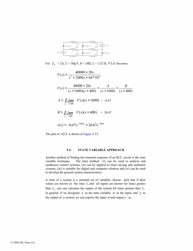
3 Ohms 4 Ohms

2 Ohms 2 Ohms

2 Ohms 4 Ohms

2 Ohms 4 Ohms

4 Ohms 3 Ohms

6 V

6 V

I1 I2

I3 I4

For I S = 2A, C = 50µ F, R = 10Ω, L = 1/32 H, V s( ) becomes

V s ss s

( )*

= ++ +

40000 202000 64 102 4

V s ss s

As

Bs

( )( )( ) ( ) ( )

= ++ +

=+

++

40000 201600 400 1600 400

A V s ssLim= +→ −1600

1600( )( ) = -6.67

B V s ssLim= +→ −400

400( )( ) = 26.67

v t e et t( ) . .= − +− −6 67 26 671600 400

The plot of v t( ) is shown in Figure 5.13.

5.4 STATE VARIABLE APPROACH

Another method of finding the transient response of an RLC circuit is the state variable technique. The later method (i) can be used to analyze and synthesize control systems, (ii) can be applied to time-varying and nonlinear systems, (iii) is suitable for digital and computer solution and (iv) can be used to develop the general system characteristics.

A state of a system is a minimal set of variables chosen such that if their values are known at the time t, and all inputs are known for times greater than t1 , one can calculate the output of the system for times greater than t1 . In general, if we designate x as the state variable, u as the input, and y as the output of a system, we can express the input u and output y as



x t Ax t Bu t( ) ( ) ( )•

= + (5.22)

y t Cx t Du t( ) ( ) ( )= + (5.23)

where

u t

u tu t

u tn

( )

( )( )..( )

=

1

2

x t

x tx t

x tn

( )

( )( )..( )

=

1

2

y t

y ty t

y tn

( )

( )( )..( )

=

1

2

and A, B, C, and D are matrices determined by constants of a system.

For example, consider a single-input and a single-output system described by the differential equation

d y tdt

d y tdt

d y tdt

dy tdt

y t u t4

4

3

3

2

23 4 8 2 6( ) ( ) ( ) ( ) ( ) ( )+ + + + =

(5.24)

We define the components of the state vector as

x t y t1( ) ( )=

x t dy tdt

dx tdt

x t21

1( ) ( ) ( ) ( )= = =•

x t d y tdt

dx tdt

x t3

2

22

2( ) ( ) ( ) ( )= = =•

x t d y tdt

dx tdt

x t4

3

33

3( ) ( ) ( ) ( )= = =•



x t d y tdt

dx tdt

x t5

4

44

4( ) ( ) ( ) ( )= = =•

(5.25)

Using Equations (5.24) and (5.25), we get

x t u t x t x t x t x t4 4 3 2 16 3 4 8 2( ) ( ) ( ) ( ) ( ) ( )•

= − − − − (5.26)

From the Equations (5.25) and (5.26), we get

x t

x t

x t

x t

x tx tx tx t

u t

1

2

3

4

1

2

3

4

0 1 0 00 0 1 00 0 0 12 8 4 3

0006

( )

( )

( )

( )

( )( )( )( )

( )

•

•

•

•

=

− − − −

+

(5.27)

or x t Ax t Bu t( ) ( ) ( )•

= + (5.28)

where

x

x t

x t

x t

x t

•

•

•

•

•

=

1

2

3

4

( )

( )

( )

( )

; A =

− − − −

0 1 0 00 0 1 00 0 0 12 8 4 3

; B =

0006

(5.29)

Since

y t x t( ) ( )= 1

we can express the output y t( ) in terms of the state x t( ) and input u t( ) as

y t Cx t Du t( ) ( ) ( )= + (5.30)

where



[ ]C = 1 0 0 0 and [ ]D = 0 (5.31)

In RLC circuits, if the voltage across a capacitor and the current flowing in an inductor are known at some initial time t, then the capacitor voltage and inductor current will allow the description of system behavior for all subsequent times. This suggests the following guidelines for the selection of acceptable state variables for RLC circuits:

1. Currents associated with inductors are state variables.

2. Voltages associated with capacitors are state variables.

3. Currents or voltages associated with resistors do not specify independent state variables.

4. When closed loops of capacitors or junctions of inductors exist in a circuit, the state variables chosen according to rules 1 and 2 are not independent.

Consider the circuit shown in Figure 5.11.

Vs

R1 R3R2

C1 C2LV1 V2

I1

y(t)

++

+

- -

-

Figure 5.11 Circuit for State Analysis

Using the above guidelines, we select the state variables to be V V1 2, , and i1 .

Using nodal analysis, we have



C dv tdt

V VR

V VR

s1

1 1

1

1 2

2

0( ) + − + − = (5.32)

Cdv t

dtV V

Ri2

2 2 1

21 0

( )+

−+ = (5.33)

Using loop analysis

V i R L di tdt2 1 31= + ( )

(5.34)

The output y t( ) is given as

y t v t v t( ) ( ) ( )= −1 2 (5.35)

Simplifying Equations (5.32) to (5.34), we get

dv t

dt C R C RV V

C RV

C Rs1

1 1 1 21

2

1 2 1 1

1 1( ) ( )= − + + + (5.36)

dv t

dtV

C RV

C RiC

2 1

2 2

2

2 2

1

2

( )= − − (5.37)

di t

dtVL

RL

i1 2 31

( ) = − (5.38)

Expressing the equations in matrix form, we get

V

Vi

C R C R C R

C R C R C

LRL

VVi

C RVs

1

2

1

1 1 1 2 1 2

2 2 2 2 2

3

1

2

1

1 1

1 1 10

1 1 1

01

1

00

•

•

•

=

− +

− −

−

+

( )

(5.39)



and the output is

[ ]yVVi

= −

1 1 01

2

1

(5.40)

MATLAB functions for solving ordinary differential equations are ODE functions. These are described in the following section.

5.4.1 MATLAB Ode Functions

MATLAB has two functions, ode23 and ode45, for computing numerical solutions to ordinary differential equations. The ode23 function integrates a system of ordinary differential equations using second- and third-order Runge-Kutta formulas; the ode45 function uses fourth- and fifth-order Runge-Kutta integration equations.

The general forms of the ode functions are

[ t,x ] = ode23 (xprime, tstart, tfinal, xo, tol,trace)

or

[ t,x ] = ode45 (xprime, tstart, tfinal, xo, tol, trace)

where

xprime is the name (in quotation marks) of the MATLAB function or m-file that contains the differential equations to be integrated. The

function will compute the state derivative vector x t( )•

given the current time t, and state vector x t( ) . The function must have 2 input arguments, scalar t (time) and column vector x (state) and the

function returns the output argument xdot x, ( ).

, a column vector of state derivatives

x t dx tdt

( ) ( )1

1•

=



tstart is the starting time for the integration

tfinal is the final time for the integration

xo is a column vector of initial conditions

tol is optional. It specifies the desired accuracy of the solution.

Let us illustrate the use of MATLAB ode functions with the following two examples.

Example 5.6

For Figure 5.2, VS = 10V, R = 10,000 Ω, C = 10µF. Find the output voltage v t0 ( ) , between the interval 0 to 20 ms, assuming v0 0 0( ) = and by (a) using a numerical solution to the differential equation; and (b) analytical solution.

Solution

From Equation (5.3), we have

C dv tdt

v t VR

o o s( ) ( )+ − = 0

thus

dv t

dtVCR

v tCR

v to s o( ) ( ) ( )= − = −100 10 0

From Equation(5.4), the analytical solution is

v t et

CR0 10 1( ) = −

−

MATLAB Script



% Solution for first order differential equation % the function diff1(t,y) is created to evaluate % the differential equation % Its m-file is diff1.m % % Transient analysis of RC circuit using ode % function and analytical solution % numerical solution using ode t0 = 0; tf = 20e-3; xo = 0; % initial conditions [t, vo] = ode23('diff1',t0,tf,xo); % the analytical solution given by Equation(5.4) is vo_analy = 10*(1-exp(-10*t)); % plot two solutions subplot(121) plot(t,vo,'b') title('State Variable Approach') xlabel('Time, s'),ylabel('Capacitor Voltage, V'),grid subplot(122) plot(t,vo_analy,'b') title('Analytical Approach') xlabel('Time, s'),ylabel('Capacitor Voltage, V'),grid

% function dy = diff1(t,y) dy = 100 - 10*y; end

Figure 5.12 shows the plot obtained using Equation (5.4) and that obtained from the MATLAB ode23 function. From the two plots, we can see that the two results are identical.



(a) (b)

Figure 5.12 Output Voltage v t0 ( ) Obtained from (a) State Variable Approach and (b) Analytical Method

Example 5.7

For Figure 5.10, if R = 10Ω, L = 1/32 H, C = 50µF, use a numerical solution of the differential equation to solve v t( ) . Compare the numerical solution to the analytical solution obtained from Example 5.5.

Solution

From Example 5.5, vC ( )0 = 20V, iL ( )0 0= , and

L

di tdt

v t

Cdv t

dti

v tR

I

LC

CL

CS

( )( )

( ) ( )

=

+ + − =0



Simplifying, we get

di tdt

v tL

dv tdt

IC

i tC

v tRC

L C

C S L C

( ) ( )

( ) ( ) ( )

=

= − −

Assuming that

x t i tx t v t

L

C

1

2

( ) ( )( ) ( )

==

We get

x tL

x t1 2

1•=( ) ( )

x tIC C

x tRC

x tS2 1 2

1 1•= − −( ) ( ) ( )

We create function m-file containing the above differential equations.

MATLAB Script

% Solution of second-order differential equation % The function diff2(x,y) is created to evaluate the diff. equation % the name of the m-file is diff2.m % the function is defined as: % function xdot = diff2(t,x) is = 2; c = 50e-6; L = 1/32; r = 10; k1 = 1/c ; % 1/C k2 = 1/L ; % 1/L k3 = 1/(r*c); % 1/RC xdot(1) = k2*x(2); xdot(2) = k1*is - k1*x(1) - k3*x(2); end



To simulate the differential equation defined in diff2 in the interval 0 ≤ t ≤ 30 ms, we note that

x iL1 0 0 0( ) ( )= = V

x vC2 0 0 20( ) ( )= =

Using the MATLAB ode23 function, we get

% solution of second-order differential equation % the function diff2(x,y) is created to evaluate % the differential equation % the name of m-file is diff2.m % % Transient analysis of RLC circuit using ode function % numerical solution t0 = 0; tf = 30e-3; x0 = [0 20]; % Initial conditions [t,x] = ode23('diff2',t0,tf,x0); % Second column of matrix x represent capacitor voltage subplot(211), plot(t,x(:,2)) xlabel('Time, s'), ylabel('Capacitor voltage, V') text(0.01, 7, 'State Variable Approach') % Transient analysis of RLC circuit from Example 5.5 t2 =0:1e-3:30e-3; vt = -6.667*exp(-1600*t2) + 26.667*exp(-400*t2); subplot(212), plot(t2,vt) xlabel('Time, s'), ylabel('Capacitor voltage, V') text(0.01, 4.5, 'Results from Example 5.5')

The plot is shown in Figure 5.13.



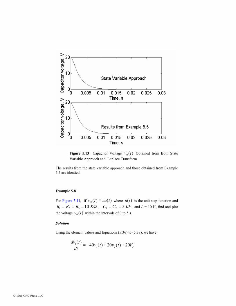
Figure 5.13 Capacitor Voltage v t0 ( ) Obtained from Both State Variable Approach and Laplace Transform

The results from the state variable approach and those obtained from Example 5.5 are identical.

Example 5.8

For Figure 5.11, if v t u tS ( ) ( )= 5 where u t( ) is the unit step function and R R R K1 2 3 10= = = Ω , C C F1 2 5= = µ , and L = 10 H, find and plot

the voltage v t0 ( ) within the intervals of 0 to 5 s.

Solution

Using the element values and Equations (5.36) to (5.38), we have

dv t

dtv t v t Vs

11 240 20 20( ) ( ) ( )= − + +



dv t

dtv t v t i t2

1 2 120 20( ) ( ) ( ) ( )= − −

di t

dtv t i t1

2 101 1000( ) . ( ) ( )= −

We create an m-file containing the above differential equations. MATLAB Script

% % solution of a set of first order differential equations % the function diff3(t,v) is created to evaluate % the differential equation % the name of the m-file is diff3.m % function vdot = diff3(t,v) vdot(1) = -40*v(1) + 20*v(2) + 20*5; vdot(2) = 20*v(1) - 20*v(2) - v(3); vdot(3) = 0.1*v(2) -1000*v(3); end

To obtain the output voltage in the interval of 0 ≤ t ≤ 5 s, we note that the output voltage

v t v t v t0 1 2( ) ( ) ( )= −

Note that at t < 0, the step signal is zero so

v v i0 2 10 0 0 0( ) ( ) ( )= = =

Using ode45 we get

% solution of a set of first-order differential equations % the function diff3(t,v) is created to evaluate % the differential equation % the name of the m-file is diff3.m % % Transient analysis of RLC circuit using state



% variable approach t0 = 0; tf = 2; x0 = [0 0 0]; % initial conditions [t,x] = ode23('diff3', t0, tf, x0); tt = length(t); for i = 1:tt vo(i) = x(i,1) - x(i,2); end plot(t, vo) title('Transient analysis of RLC') xlabel('Time, s'), ylabel('Output voltage')

The plot of the output voltage is shown in Figure 5.14.

Figure 5.14 Output Voltage 10 V

10,000 Ohms

LR

VLPL



SELECTED BIBLIOGRAPHY 1. MathWorks, Inc., MATLAB, High-Performance Numeric Computation Software, 1995. 2. Biran, A. and Breiner, M. MATLAB for Engineers, Addison-Wesley, 1995. 3. Etter, D.M., Engineering Problem Solving with MATLAB, 2nd

Edition, Prentice Hall, 1997. 4. Nilsson, J.W., Electric Circuits, 3rd Edition, Addison-Wesley Publishing Company, 1990. 5. Vlach, J.O., Network Theory and CAD, IEEE Trans. on Education, Vol. 36, No. 1, Feb. 1993, pp. 23 - 27. 6. Meader, D. A., Laplace Circuit Analysis and Active Filters, Prentice Hall, New Jersey, 1991.

EXERCISES

5.1 If the switch is opened at t = 0, find v t0 ( ) . Plot v t0 ( ) between the time interval 0 ≤ t ≤ 5 s.

30V

20 kilohms 10 kilohms

1 microfarads40 kilohms

t = 0

Vo(t)

Figure P5.1 Figure for Exercise 5.1



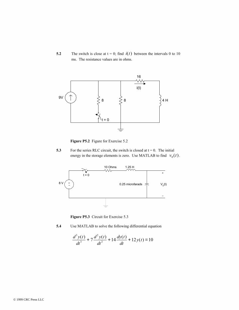
5.2 The switch is close at t = 0; find i t( ) between the intervals 0 to 10 ms. The resistance values are in ohms.

9V8 8

16

4 H

t = 0

i(t)

Figure P5.2 Figure for Exercise 5.2 5.3 For the series RLC circuit, the switch is closed at t = 0. The initial

energy in the storage elements is zero. Use MATLAB to find v t0 ( ) .

10 Ohms 1.25 H

0.25 microfarads8 V Vo(t)

t = 0

Figure P5.3 Circuit for Exercise 5.3

5.4 Use MATLAB to solve the following differential equation

d y t

dtd y t

dtdy t

dty t

3

3

2

27 14 12 10( ) ( ) ( ) ( )+ + + =



with initial conditions

y( )0 1= , dy

dt( )0 2= ,

d ydt

2

20 5( ) =

Plot y(t) within the intervals of 0 and 10 s. 5.5 For Figure P5.5, if V u tS = 5 ( ), determine the voltages V1(t), V2(t),

V3(t) and V4(t) between the intervals of 0 to 20 s. Assume that the initial voltage across each capacitor is zero.

VS

1 kilohms

1pF

V1 1 kilohms1 kilohms1 kilohms

4pF3pF2pF

V4 V3 V2

Figure P5.5 RC Network

5.6 For the differential equation

d y t

dtdy t

dty t t t

2

2 5 6 3 7( ) ( )

( ) sin( ) cos( )+ + = +

with initial conditions y( )0 4= and dy

dt( )0 1= −

(a) Determine y t( ) using Laplace transforms.

(b) Use MATLAB to determine y t( ) .

(c) Sketch y t( ) obtained in parts (a) and (b).

(d) Compare the results obtained in part c.



attia, john okyere. “ transient analysis.” electronics and circuit analysis...

Documents