audio recognition with distributed wireless sensor networks
TRANSCRIPT

Audio Recognition with Distributed Wireless Sensor Networksby
Bidong ChenB.Sc. University of Victoria, 2004B.Eng. Zhejiang University, 1996
A Thesis Submitted in Partial Fulfillment of the Requirementsfor the Degree of
MASTER OF SCIENCE
in the Department of Computer Science
c© Bidong Chen, 2010University of Victoria
All rights reserved. This thesis may not be reproduced in whole or in part byphotocopy or other means, without the permission of the author.

ii
Audio Recognition with Distributed Wireless Sensor Networks
by
Bidong Chen
B.Sc. University of Victoria, 2004
B.Eng. Zhejiang University, 1996
Supervisory Committee:
Dr. Kui Wu, Co-Supervisor (Department of Computer Science)
Dr. George Tzanetakis, Co-Supervisor (Department of Computer Science)
Dr. Jianping Pan, Outside Member (Department of Computer Science)

iii
Supervisory Committee:
Dr. Kui Wu, Co-Supervisor (Department of Computer Science)
Dr. George Tzanetakis, Co-Supervisor (Department of Computer Science)
Dr. Jianping Pan, Outside Member (Department of Computer Science)
ABSTRACT
Recent technique advances have made sensor nodes to be smaller, cheaper and more pow-
erful. Compared with traditional centralized sensing systems, wireless sensor networks are
very easy to deploy and can be deployed densely. They have a better sensing coverage
and provide more reliable information delivery. Those advantages make wireless sensor
networks very useful in a wide variety of applications. As one of active research areas,
acoustic monitoring with wireless sensor networks is still new, and very few applications
can recognize human voice, discriminate human speech and music, or identify individual
speakers. In this thesis work, we designed and implemented an acoustic monitoring system
with a wireless sensor network to classify human voice versus music. We also introduce a
new, effective sound source localization method, using Root Mean Square (RMS) detected
by different nodes of a wireless sensor network to estimate the speaker’s location. The ex-
perimental results show that our approaches are effective. This research could form a basis
for further developing speech recognition, speaker identification, even emotion detection
with wireless sensor networks.

iv
Table of Contents
Spervisory Committee ii
Abstract iii
Table of Contents iv
List of Tables vii
List of Figures viii
List of Abbreviations ix
Acknowledgment x
Dedication xi
1 Introduction 1
1.1 Wireless Sensor Networks . . . . . . . . . . . . . . . . . . . . . . . . . . 1
1.2 Acoustic Monitoring with Wireless Sensor Network . . . . . . . . . . . . 2
1.3 The Goal and the Challenges . . . . . . . . . . . . . . . . . . . . . . . . . 3
1.4 A Sketch Introduction of Our System . . . . . . . . . . . . . . . . . . . . 5
1.5 Contributions . . . . . . . . . . . . . . . . . . . . . . . . . . . . . . . . . 8
2 Related Work 10
2.1 Acoustic Monitoring with Wireless Sensor Networks . . . . . . . . . . . . 10
2.2 Speech/Music Classification . . . . . . . . . . . . . . . . . . . . . . . . . 12

Table of Contents v
2.3 Speech Recognition with Wireless Sensor Network . . . . . . . . . . . . . 13
3 System Description 15
3.1 The Framework of Audio Recognition System . . . . . . . . . . . . . . . 15
3.2 Sampling . . . . . . . . . . . . . . . . . . . . . . . . . . . . . . . . . . . 16
3.3 Activity Detection . . . . . . . . . . . . . . . . . . . . . . . . . . . . . . 16
3.4 Framing . . . . . . . . . . . . . . . . . . . . . . . . . . . . . . . . . . . . 17
3.5 Fast Fourier Transform (FFT) . . . . . . . . . . . . . . . . . . . . . . . . 17
3.6 Feature Extraction /Transmission . . . . . . . . . . . . . . . . . . . . . . 18
3.6.1 Spectral Centroid . . . . . . . . . . . . . . . . . . . . . . . . . . 18
3.6.2 Spectral Rolloff . . . . . . . . . . . . . . . . . . . . . . . . . . . 19
3.6.3 RMS . . . . . . . . . . . . . . . . . . . . . . . . . . . . . . . . . 19
3.7 TinyOS and nesC . . . . . . . . . . . . . . . . . . . . . . . . . . . . . . . 20
3.8 Classification . . . . . . . . . . . . . . . . . . . . . . . . . . . . . . . . . 20
3.8.1 Bayesian Networks . . . . . . . . . . . . . . . . . . . . . . . . . 21
3.8.2 K-Nearest Neighbors . . . . . . . . . . . . . . . . . . . . . . . . 21
3.8.3 Decision Tree (D-Tree) . . . . . . . . . . . . . . . . . . . . . . . 23
3.8.4 Support Vector Machines (SVM) . . . . . . . . . . . . . . . . . . 24
3.8.5 The Classification of Speech and Music . . . . . . . . . . . . . . . 25
3.8.6 Speaker Localization . . . . . . . . . . . . . . . . . . . . . . . . . 25
4 Evaluation 29
4.1 Speech and music discrimination . . . . . . . . . . . . . . . . . . . . . . 30
4.2 Results on estimating speaker’s location . . . . . . . . . . . . . . . . . . . 31
5 Lessons Learned 37
5.1 Memory constraint . . . . . . . . . . . . . . . . . . . . . . . . . . . . . . 37
5.2 No continuous sampling . . . . . . . . . . . . . . . . . . . . . . . . . . . 37
5.3 Threshold value selection . . . . . . . . . . . . . . . . . . . . . . . . . . 38

Table of Contents vi
5.4 Synchronization . . . . . . . . . . . . . . . . . . . . . . . . . . . . . . . 38
5.5 Validation . . . . . . . . . . . . . . . . . . . . . . . . . . . . . . . . . . . 39
5.6 Noise . . . . . . . . . . . . . . . . . . . . . . . . . . . . . . . . . . . . . 39
5.7 Select classification algorithm . . . . . . . . . . . . . . . . . . . . . . . . 39
6 Conclusion 41
6.1 wireless sensor networks . . . . . . . . . . . . . . . . . . . . . . . . . . . 41
6.2 Contributions . . . . . . . . . . . . . . . . . . . . . . . . . . . . . . . . . 43
6.3 Future works . . . . . . . . . . . . . . . . . . . . . . . . . . . . . . . . . 44
Bibliography 46

vii
List of Tables
Table 4.1 Weka algorithms and parameters used in classification experiments . 29
Table 4.2 Classification accuracy in a system with three sensor nodes using two
features . . . . . . . . . . . . . . . . . . . . . . . . . . . . . . . . . . . . 31
Table 4.3 Classification accuracy in a system with two sensor nodes using two
features . . . . . . . . . . . . . . . . . . . . . . . . . . . . . . . . . . . . 32
Table 4.4 Classification accuracy in a system with one sensor node using two
features . . . . . . . . . . . . . . . . . . . . . . . . . . . . . . . . . . . . 32
Table 4.5 Performance drops when reducing the number of sensors . . . . . . . 33
Table 4.6 Classification accuracy in a system with three sensor nodes using one
feature . . . . . . . . . . . . . . . . . . . . . . . . . . . . . . . . . . . . . 33
Table 4.7 Classification accuracy in a system with three sensor nodes using one
feature . . . . . . . . . . . . . . . . . . . . . . . . . . . . . . . . . . . . . 34
Table 4.8 Classification accuracy in estimating the speaker’s location . . . . . . 36
viii
List of Figures
Figure 1.1 A Mica2 sensor mote from Crossbow Inc. . . . . . . . . . . . . . . 2
Figure 1.2 Wireless sensor network architecture [1] . . . . . . . . . . . . . . . 5
Figure 1.3 Flowchart for audio recognition . . . . . . . . . . . . . . . . . . . . 7
Figure 3.1 Flowchart for an audio recognition system with wireless sensor net-
work . . . . . . . . . . . . . . . . . . . . . . . . . . . . . . . . . . . . . 15
Figure 3.2 A simple Bayesian network . . . . . . . . . . . . . . . . . . . . . . 22
Figure 3.3 A simple example of the K-NN algorithm . . . . . . . . . . . . . . 23
Figure 3.4 An example of D-Tree . . . . . . . . . . . . . . . . . . . . . . . . . 24
Figure 3.5 Flowchart for speech and music classification . . . . . . . . . . . . 26
Figure 3.6 Flowchart for estimating speaker location . . . . . . . . . . . . . . 28
Figure 4.1 Estimate speaker’s location . . . . . . . . . . . . . . . . . . . . . . 35
Figure 4.2 chart of RMS . . . . . . . . . . . . . . . . . . . . . . . . . . . . . 35

ix
List of Abbreviations
ADT Analog-to-Digital Converter
B-Net Bayesian Networks
DAG Directed Acyclic Graph
DFT Discrete Fourier Transform
DSP Digital Signal Processing
DTW Dynamic Time Warping
D-tree Decision Tree
FFT Fast Fourier Transform
K-NN K-nearest Neighbors Algorithm
LDA Linear Discriminant Analysis
MFCC Mel-scaled Frequency Cepstral Coefficients
PC Personal Computer
RMS Root Mean Square
SVM Support Vector Machines
TOA Time of Arrival
UCLA University of California, Los Angeles
WOLA Weighted Overlap-add

x
Acknowledgment
I would like to express my deep appreciation to my supervisors, Dr. Kui Wu and Dr.
George Tzanetakis, for their patience, support, guidance and encouragement in all the time
of research and writing of this thesis. I would like to thank my examining committee
members, Dr. Jianping Pan and Dr. Issa Traore, for their valuable effort.
I would also like to thank my friends and my family who have privided constant support
and encouragement to me throught this long process.

xi
Dedication
To my family

Chapter 1
Introduction
1.1 Wireless Sensor Networks
Recent technique advance in integrated circuit, wireless communication, and Micro Electro-
Mechanical System, has made it feasible to construct very small sensor nodes, which are
cheap, consume low energy, and have the capabilities of signal processing and wireless
communication [2]. As shown in Fig. 1.1, the size of such sensor nodes could be as small
as several cubic centimeters, and as such they sometimes are also called sensor motes.
When many sensor motes are interconnected with wireless communication, they form an
autonomic network system, called a wireless sensor network.
Compared to a single sensor system, wireless sensor networks have many advantages.
First, they are very easy to deploy. For instance, sensor motes can be dropped by air flight
into a forest, and they automatically communicate with each other to form a network suit-
able for forest fire monitoring. Second, due to the low cost of each individual sensor, sensor
nodes can be deployed very densely. In this way, although the processing capability of each
sensor node might be limited, the aggregate of many sensor nodes actually possesses non-
trivial computational power. Third, when multiple sensors work together, the information
redundancy among the sensors and the redundant communication channels in the networks
enable a better sensing coverage and provide more reliable information delivery. The above
advantages make wireless sensor networks much more powerful than traditional centralized
sensing systems. It has become a clear trend that wireless sensor networks are being used in

1.2 Acoustic Monitoring with Wireless Sensor Network 2
Figure 1.1. A Mica2 sensor mote from Crossbow Inc.
a wide range of applications, including environmental monitoring, condition-based mainte-
nance, habitat monitoring, military surveillance, inventory tracking, health care, and much
more [2, 3, 4].
1.2 Acoustic Monitoring with Wireless Sensor Network
Acoustic signals contain a great deal of information about their generating sound sources.
Due to this reason, acoustic monitoring based on wireless sensor networks has received
much attention and has been used in a lot of applications. For example, a research group
in UCLA [5] built an acoustic habitat-monitoring sensor network, which recognizes and
locates specific animal calls in real time. Simon et al. [6] developed a system based on ad-
hoc wireless sensor networks to detect and locate shooters in urban environment. Phadke et
al. [7] designed an embedded speech recognition system, which is capable of recognizing

1.3 The Goal and the Challenges 3
a spoken word from a small vocabulary of about 10-15 words. Underwater acoustic moni-
toring is being used to study the distribution of large whales in the open oceans [8]. Hydro
acoustic monitoring system has been applied to detect and precisely locate small undersea
earthquakes [9]. A wireless sensor network using acoustic sensors can be used to monitor
volcanic eruption [10]. It can also be used in monitoring unstable cliffs, slopes, and rock
faces [11].
1.3 The Goal and the Challenges
Although many acoustic monitoring applications have been developed, acoustic monitor-
ing with wireless sensor networks is still new, and very few systems can recognize human
voice, discriminate human speech and music, or identify individual speakers. These func-
tionalities are important, since they are indispensable in many new acoustic monitoring
applications. For example, speaker identification can be used in a “smart conference hall”
application, which needs to identify and locate speakers through an acoustic monitoring
system deployed in a large conference place; Speech/music discrimination can be used
in hearing aid instruments that can automatically switch between different hearing aid al-
gorithms based on the current environment. In this thesis, we explore the possibility of
discriminating human speech and music, and localizing speakers with wireless sensor net-
works.
To achieve the above goal, we need to explore and integrate knowledge from multi-
ple disciplines, particularly on audio recognition, machine learning, and wireless sensor
networking. The project poses the following research challenges that this thesis will ad-
dress [3, 5, 12, 13].
• Limited computational capability. Due to the small size, current sensor nodes pro-
vide only very limited processing power. For example, the MICA2 mote uses a slow
8 MHz Atmel 128 microprocessor. The limited processing capability renders existing
audio recognition algorithms impossible to implement on individual sensors. Audio

1.3 The Goal and the Challenges 4
recognition algorithms are frequently used in the application of speech recognition,
speaker identification, and music classification. They generally need to compare
sounds, with the help of the extraction of sound features. Many applications have
been developed for automatic classification of speech or music, but most of them
are only suitable to run over powerful PCs, using the samples from a single sensor
(e.g., a single microphone). We instead focus on designing and implementing an
audio recognition system with the abundant information from multiple collaborative,
distributed sensor nodes.
• Limited storage space. The MICA2 mote has only 4 kB data memory space. With
such a limited space, it is unrealistic to sample the sound in a high sample rate,
because otherwise the large number of samples will quickly overflow the buffer. With
limited sample size, it is a big challenge to get the accurate and effective feature set
suitable for different audio classification tasks. As a result, the feature extraction
algorithms implemented over sensor node should have not only low computational
complexity but also low memory requirements.
• Limited bandwidth. The scarce communication bandwidth greatly limits data trans-
mission between a sensor node and the processing center (also called the base station.
It is a laptop in our system). For instance, the sensor nodes in our system, MICA2
motes, have the current draw of 27 mA when transmitting with maximum power and
the maximum bandwidth of 38.4 kbps only. The bandwidth bottleneck requires that
we must carefully balance the overhead of communication and computation. Send-
ing all raw samples from a sensor node may not be a wise choice. Instead, it is better
to pre-process the data in sensors and only transmit feature information to reduce
bandwidth overhead.
• Limited energy supply. The sensor nodes are not connected to any wired energy
sources. They are usually powered by battery but are expected to work for several
months to one year without recharging. The communication requires much higher
energy consummation compared to data processing. In order to extend the lifetime
1.4 A Sketch Introduction of Our System 5
of battery-powered sensors, communication needs to be minimized as much as pos-
sible. Such a requirement asks us to avoid transmitting raw data to the base station
by processing data (e.g., data compression, feature extraction, etc.) locally before
sending them to the base station.
1.4 A Sketch Introduction of Our System
We tackle the above challenges in this thesis. To help quickly understand our method,
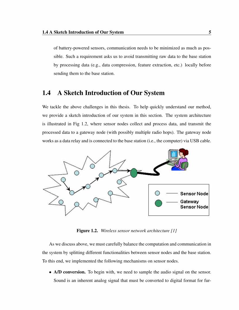
we provide a sketch introduction of our system in this section. The system architecture
is illustrated in Fig 1.2, where sensor nodes collect and process data, and transmit the
processed data to a gateway node (with possibly multiple radio hops). The gateway node
works as a data relay and is connected to the base station (i.e., the computer) via USB cable.
Figure 1.2. Wireless sensor network architecture [1]
As we discuss above, we must carefully balance the computation and communication in
the system by splitting different functionalities between sensor nodes and the base station.
To this end, we implemented the following mechanisms on sensor nodes.
• A/D conversion. To begin with, we need to sample the audio signal on the sensor.
Sound is an inherent analog signal that must be converted to digital format for fur-

1.4 A Sketch Introduction of Our System 6
ther processing. Audio recognition begins with the digital samples of audio signals.
Because of the limitation of the memory size, we need to set an appropriate sampling
rate which can produce records useful for Fast Fourier Transform (FFT) and fea-
ture extraction. Eight-bit samples at an 8 kHz sampling rate is the minimum quality
requirement for recorded speech that can be understood by humans [14].
• FFT. We need to implement the Fast Fourier Transform (FFT) algorithm on the sen-
sor node because FFT forms the basis of most audio feature extraction algorithms.
FFT calculates the frequency components of a signal. After FFT, a sampled sig-
nal is transformed to the frequency domain. Then we can easily observe the main
frequencies in our sampled signals are. Based on the result of FFT, we can further
implement the feature extraction algorithms on the sensor. Sensor nodes could keep
these features in a buffer, and send them to the base station when the buffer is nearly
full.
• Feature extraction. The extraction of feature vector from audio signals is the ba-
sis of automatic audio recognition system. Because of the limited bandwidth and
constrained resources on processing and storage capacity, a sensor node cannot sam-
ple human voice in a high rate, nor could it store a large number of samples in its
memory. In addition, transmitting raw sample data will cause too large communica-
tion overhead. We need to implement a simple, memory efficient feature extraction
algorithm over sensor nodes.
When sensor nodes transmit the extracted audio feature values to the base station, fur-
ther processing will be performed on the base station, including training, and classifying
sound features. Fig. 1.3 shows the basic operations in our audio recognition system with
wireless sensor network. Note that Fig. 1.3 is just a high-level flow chart. The details on
each individual steps, particularly on “Feature Extraction” and “Further Signal Processing”,
will be disclosed in Chapter 3.

1.4 A Sketch Introduction of Our System 7
Sampling
Detection and framing
256-point FFT
Feature extraction
Collect enoughfeatures
NO
YES
Speech/Music
Sensor node
Base station
Further Signal Processing
Classifiers
Each sensor node transmitsdata to base station by radio
Figure 1.3. Flowchart for audio recognition

1.5 Contributions 8
1.5 Contributions
In this thesis, we made the following contributions:
• Design and implementation of an acoustic monitoring system that extracts sound
features in a distributed fashion. We compute low-level numerical features from
the audio input at each sensor node, which are then transmitted wirelessly to the base
station. We then perform further processing of the features, using machine learn-
ing algorithms. Since each sensor contributes a set of audio features from different
places, our approach enables good audio recognition even when some of the sensors
are not working optimally. The transmission of features instead of raw sample data
can significantly reduce bandwidth cost and is resilient to ordering errors.
• Diverse audio recognition functionality. We use the wireless sensor network to
automatically classify different types of audio sources. In this thesis, we research on
how to classify human voice versus music. This research may lay the foundations for
more complex tasks, like emotion recognition and speaker identification.
• Effective sound source localization method. We study a new approach that uses
Root Mean Square (RMS) of a set of audio sample values to measure the energy of
sound detected by a sensor and to estimate the speaker’s location. Unlike locating a
target using the time difference of arrival, this approach does not need complicated
computation, and can be easily setup in a small area such as a meeting room. Each
sensor node records the sound and computes the RMS locally, and then sends the
extracted features to base station. The base station, after collecting enough data, uses
machine learning algorithms to estimate the location of the speaker. Our experimen-
tal test shows that this method is effective and performs very well.
The rest of the thesis is organized as follows. Chapter 2 reviews the related work. In
Chapter 3, we introduce in detail our design of the automatic audio signal classifier with
wireless sensor network. In Chapter 4, we test the system and evaluate the testing results.
The lessons learned from this project is described in Chapter 5. Finally, we introduce future

1.5 Contributions 9
work and conclude the thesis in Chapter 6.

10
Chapter 2
Related Work
Many audio recognition systems, including speech recognition, speaker identification, speech/music
discrimination, emotion recognition, etc., have been developed over Personal Computers
(PC) [15]. The performance of such systems varies, and improving the accuracy of audio
recognition systems has been a long-standing challenge since the early days of comput-
ing. Equipped with multiple geographically scattered sensors, wireless sensor networks
may open a big opportunity to build an audio recognition system better than ever. Nev-
ertheless, audio recognition with wireless sensor networks is still new. The potential of
using distributed wireless sensor networks has not been fully explored, due to some dif-
ficulties introduced in the first Chapter. To help better understand our contributions, we
introduce existing research efforts on acoustic monitoring with wireless sensor networks in
this chapter.
2.1 Acoustic Monitoring with Wireless Sensor Networks
Wireless sensor networks have a variety of applications. Examples include environmental
monitoring, habitat monitoring, seismic detection, military surveillance, inventory track-
ing, smart spaces, etc. Recently, researchers try to push the limit of tiny little sensors to
perform complex monitoring tasks. One such effort is to use wireless sensor networks for
audio recognition. Along the line, several applications have been developed to recognize a
specific animal, locate a target, or recognize human speech.

2.1 Acoustic Monitoring with Wireless Sensor Networks 11
A research group in UCLA has developed an acoustic habitat-monitoring sensor net-
work that recognizes and locates specific animal calls in real time [5]. They propose a
system architecture and a set of lightweight collaborative signal processing algorithms to
achieve real-time detection, with the goal to minimize the inter-node communication and
maximize the system lifetime. In particular, the target classification is based on spectro-
gram pattern matching while the target localization is based on beamforming using time
difference of arrival.
Researchers in Vanderbilt University have built a system based on an ad-hoc wireless
sensor network to spot shooters precisely in urban environments [6]. The system utilizes
an ad-hoc wireless sensor network built with cheap sensor nodes. After deployment, the
sensor nodes can synchronize their time, perform self-localization and wait for acoustic
events. The sensors are able to detect muzzle blasts and acoustic shockwaves, and measure
their time of arrival (TOA). Utilizing a message routing service, the TOA measurements are
delivered to the base station, typically a laptop computer, where a sensor fusion algorithm
is executed to estimate the shooter’s location.
Note that in the above two systems, target localization is done with the analysis of TOA
values. These methods are sensitive to errors in packet orders and the inaccuracy in system
clocks. To overcome the problem, in this thesis we explore a totally different method that
estimates the energy of audio waves.
In Australia, a group of researchers [16] are using a wireless sensor network in Queens-
land’s Springbrook National Park to monitor the recovery of the regenerating rainforest
from previous agricultural grassland. Currently, the system is extended to include new
monitoring tasks such as frog monitoring, because frog populations are often a good bio-
indicator of the health of waterway ecosystems. The frog monitoring is fulfilled with acous-
tic monitoring that recognizes, records, and classifies frog vocalizations [17].

2.2 Speech/Music Classification 12
2.2 Speech/Music Classification
Speech/music classification is one of the most interesting and useful techniques in audio
signal classification. For instance, speech/music classification and discrimination can be
used as a first stage in an automatic speech recognition system. They can also be used
to recognize the genre of music [18]. As recognizing and classifying audio signals (e.g.,
human speech, different animal sounds) is one of the most sophisticated human abilities,
the implementation of such intelligence in a monitoring system is clearly critical for the
success of many applications.
In recent years, many methods have been proposed to automatically discriminate speech
and music signals. Saunders [19] introduced a real-time speech/music discriminator that
was used to automatically classify audio content of FM radio channels. In the system,
zero-crossings rate and energy related features are calculated for 16 msec frames, and then
the statistical features were calculated in every 2.4 seconds window. The classifier in the
system was a multivariate-Gaussian classifier. Panagiotakis and Tziritas [20] designed a
speech/music discriminator that uses Root Mean Squares (RMS) and zero-crossings cal-
culation. They computed the normalized RMS and the probability of null zero-crossings.
The decision was made by comparing the results with a threshold value. Scheirer and
Slaney [21] proposed a solution to discriminate speech from various types of music by us-
ing features such as spectral centroid, spectral flux, zero-crossing rate, 4 Hz modulation
energy, and the percentage of low-energy frames. Four different classifiers have been used
in the evaluation of the performance. Williams and Ellis [22] used features, which are ob-
tained with the output results from an acoustic phone classifier, to separate speech from
music material. In [23], Cortizo et al. presented a speech/music classification method that
uses Fisher linear discriminant analysis (Fisher LDA) for each feature extracted from audio
signals. The above approaches use supervised learning and thus require a large amount
of training data and pre-determined audio classes to train their classifiers. In the contrast,
in [24], a fast and effective unsupervised clustering method for speech/music classification

2.3 Speech Recognition with Wireless Sensor Network 13
has been presented. The method is inspired by the classical K-means algorithms and is
based on one-class support vector description of a dataset.
In the existing published work, none of the proposed systems are implemented in a
distributed network using resource constrained wireless sensors. Unlike previous work, in
this thesis we must achieve a good balance between algorithm complexity, performance,
and resource limitation in our audio signal classifier.
2.3 Speech Recognition with Wireless Sensor Network
From Section 2.1, we can see that several acoustic monitoring systems with wireless sen-
sor networks have been developed. Nevertheless, none of them is particularly targeted at
human speech recognition as the main design goal. Although the methodology in human
speech recognition and other types of audio recognition (e.g., animal sounds or sounds
from gun shotting) is similar, the different project goals have significant impact on the se-
lection of an appropriate feature set suitable for the particular task. In this section, we
review the methods that have been used in the particular domain of speech recognition and
speech/music classification.
In [25], an efficient filter bank technique, called WOLA (Weighted Overlap-add), was
used as the front-end for automatic speech recognition. This approach leads to very low-
cost implementation of signal processing algorithms suitable for a low-resource system.
Cornu and Sheikhzadeh [12] demonstrate the possibility of implementing voice recogni-
tion based services for mobile users. They described the implementation of the complete
digital Signal Processing (DSP) front-end algorithms, including feature extraction, feature
compression and multi-framing, on a DSP system designed specifically for speech pro-
cessing on a mobile device with very little power and very limited CPU resources. A team
form IIT Bombay [7] implemented an embedded speech recognition system to recognize a
spoken word from a template of 10− 15 words. This is a speaker-dependent speech recog-
nition system, but it has only a very small vocabulary. The feature extraction is based on

2.3 Speech Recognition with Wireless Sensor Network 14
modified Mel-scaled Frequency Cepstral Coefficients (MFCC), and the template matching
method employs Dynamic Time Warping (DTW). Shen [26] designed a wireless sensor
network suitable for automatic real-time speech recognition. He presented the key design
steps, including the definition of the network topology, protocol design, implementation of
the embedded speech recognition algorithm, and distribution of computation and commu-
nication tasks.

15
Chapter 3
System Description
3.1 The Framework of Audio Recognition System
Fig. 3.1 shows the basic operations that are part of the audio recognition system with a
wireless sensor network. Note that the operations of sampling, activity detection, framing,
FFT, feature extractions are performed on sensor nodes, and the task of classification is
done on the base station (a laptop in our case). We explain each individual operation in
detail in the following sections.
Sampling Activity Detection Framing
FFTFeature extractionClassificationResult
Voice input
Figure 3.1. Flowchart for an audio recognition system with wireless sensor network

3.2 Sampling 16
3.2 Sampling
Automatic audio recognition system starts with sampling the acoustic signals. In our sys-
tem, we employ a sampling frequency of 8 KHz. This sample rate is good enough for
human voice, but may be a bit low for music. Because of the limited memory size and
limited computational resource of sensor nodes, a high sampling frequency, e.g., 16 KHZ,
may quickly end up with buffer overflow and thus is not suitable. The value of 8 KHz
sampling rate is selected to make a good balance between sampling rate and the limited
resources. We use an 8-bit analog-to-digital converter (ADC) on the sensor node to sample
and convert sensed signals from an acoustic sensor.
3.3 Activity Detection
The system needs to automatically decide when it should start recording speech or music.
This feature is especially important in saving energy consumption on unnecessary process-
ing (e.g., feature extraction). It also greatly facilitates the collaboration of multiple sensor
nodes. In our project, after the system is initialized, sensor nodes keep capturing samples
from background noise and calculate the Root Mean Square (RMS) (refer to Section 3.6)
for these samples. We set a predefined threshold 1 for the RMS. The samples that have a
RMS value less than the threshold will be treated as background noise or silence. If the
samples’ RMS value exceeds the threshold, the sensor node records the speech or music
until the buffer, the size of which is 4 Kb in MICA2 motes, is filled. Then the acoustic data
are then passed to the next step for further signal processing and features extraction.
1The threshold value is set to 0.02 based on our experimental observation in an office environment at
night. This value is good enough for all sensor nodes to detect speech or music. Also, it is not too close to
the RMS value for the background silence, so backgroud noise would not cause the sensors to start collecting
data by mistake.
3.4 Framing 17
3.4 Framing
Once the system is triggered to process a block 4K samples, the block of samples is first
partitioned into 20 overlapping frames, where each frame consists of 256 samples.
3.5 Fast Fourier Transform (FFT)
When we try to identify a person, we usually describe the person’s age, height, weight, the
color of eyes, the color of hair, and so on, and hopefully these features can help “uniquely”
identify the person. Similarly, to build an audio recognition system, we also need to find
the features of the audio content, which are representative and can capture the “unique”
pattern in the audio content. The most important features for this purpose are usually the
frequency/magnitude values in the audio source, and as such we need to transform samples
obtained with the microphone sensors from the time domain to the frequency domain.
Fourier transform is exactly for this purpose. In practice, we usually use a specific kind of
Fourier transform, discrete Fourier transform (DFT).
Since wireless sensor nodes have only limited computational resource, it will be inef-
ficient and very hard to implement DFT directly on the sensor nodes. Instead, we need an
efficient algorithm to compute DFT, and thus we use Fast Fourier Transform (FFT). FFT
includes a group of distinct algorithms. In our system, we apply a 256-point FFT on each
frame. The algorithm we implemented is the real fast Fourier transform algorithm [27].
We can then use the output of FFT to construct desirable features to represent the audio
content. These features will be described in the next section. With the features selected, we
then use machine learning techniques to build up and train an audio classifier for various
recognition tasks.

3.6 Feature Extraction /Transmission 18
3.6 Feature Extraction /Transmission
In order to alleviate the problems caused by the limited resources on communication, com-
putation, and memory, we should process the signal locally on the sensor node, and only
transmit the extracted features to the base station. To this end, we need to define proper
features in the audio signals. Selecting suitable features is the base that leads to a good au-
dio signal recognition system. The objective of feature extraction is to obtain a numerical
representation which can be used to characterize the audio signal. Once the features are
extracted and transmitted to the base station, standard machine learning techniques such as
those introduced in Section 3.8 can be applied to classify the type of audio sources [18].
The following features are used in our system.
3.6.1 Spectral Centroid
With FFT, we can obtain the magnitude value at a frequency (more specifically, a dis-
cretized frequency range). The spectral centroid is defined as the center of gravity of mag-
nitude spectrum of FFT.
Ct =
N∑n=1
Mt[n]∗n
N∑n=1
Mt[n]
Where Mt[n] is the magnitude of the Fourier Transform at frame t and frequency bin
n. In our implementation, we apply a 256-point FFT on each frame, so the number of fre-
quency bins (N ) is set to 128 and the frequency range is 64 HZ in each frequency bin. Spec-
tral centroid corresponds to how bright the sound is and the pitch of the sound. Brighter
and higher pitches have higher values of spectral centroid [18].
The intuitive meaning of spectral centroid is to characterize where the “center of mass”
of the spectrum is. Perceptually, this value is closely related to the “brightness”’ of the
sound. Clearly, the “brightness” of the sound is a good feature we should capture.

3.6 Feature Extraction /Transmission 19
3.6.2 Spectral Rolloff
Spectral rolloff is another measure of spectral shape [18]. It is defined as the α-quantile
of the total energy in the audio signals. In other words, it is the frequency under which a
fraction of the total energy is found. In our system, we define the fraction value as 85%,
since this is a commonly-used value in many applications. Assume that the spectral rolloff
is Rt, we have the following relationship:
maxM{
M∑n=1
Mt[n]/N∑
n=1
Mt[n]} ≤ 0.85,
where M < N and the frequency value in the frequency bin M is Rt.
Clearly, based on spectral rolloff, we can find the frequency value under which the
majority (e.g., 85%) of the total energy resides.
3.6.3 RMS
RMS (Root Mean Square) is the square root of the arithmetical average of a set of squared
instantaneous audio sample values in a frame.
RMS =
√N∑i=1
M2[i]
N,
where N is the total number of samples and the M [i] is the i-th sample value in the
set. Note that no FFT is required in the calculation of RMS. Intuitively, the RMS is used to
measure the energy of sound detected by sensor.
We have observed that the above three features are critical and effective to capture the
property of audio signals for our later classification tasks.
After feature extraction, the sensor node starts sending the features to base station
through wireless communication. Each sensor has a unique ID, and this ID is used in
each packet to tell the base station where the message comes from.
3.7 TinyOS and nesC 20
3.7 TinyOS and nesC
In our system, all those sampling, framing, FFT, and features extraction will be imple-
mented on sensor nodes, MICA2, based on the open-source TinyOS operating system. The
TinyOS system, libraries, and applications are written in nesC, a new language for program-
ming structured component-based applications. The nesC language is primarily intended
for embedded systems such as sensor networks. nesC has a C-like syntax, but supports
the TinyOS concurrency model, as well as mechanisms for structuring, naming, and link-
ing together software components into robust network embedded systems. The principal
goal is to allow application designers to build components that can be easily composed into
complete, concurrent systems, and yet perform extensive checking at compile time [28].
TinyOS defines a number of important concepts that are expressed in nesC. First, nesC
applications are built out of components with well-defined, bidirectional interfaces. Sec-
ond, nesC defines a concurrency model, based on tasks and hardware event handlers, and
detects data races at compile time [28].
3.8 Classification
The base station is responsible for collecting features sent from sensor nodes in the system.
Machine learning algorithms are applied to train the system to classify the audio signal type.
In our system, four supervised learning algorithms are selected to evaluate the performance:
Bayesian networks (B-Net), K-nearest neighbors algorithm (K-NN), decision tree (D-tree),
and Support Vector Machines (SVM). In the following, we briefly introduce the basic idea
behind these machine learning methods to help better understand our system. More details
of these algorithms can be found in [29].

3.8 Classification 21
3.8.1 Bayesian Networks
A Bayesian network (B-Net) is a probabilistic graphical model that represents a set of ran-
dom variables and their conditional dependencies via a directed acyclic graph (DAG). A
simple but classical example of B-Net is shown in Fig. 3.2. When used together with statis-
tical techniques, B-Net has several advantages for data analysis, which make it particularly
powerful in different machine learning tasks. First, because the model encodes the depen-
dencies among different random variables, B-Net can easily handle the cases when some
data are missing. Second, because the dependencies among random variables actually cap-
ture the causal relationships, B-Net is very helpful in the prediction of consequences of
parameter changes (i.e., intervention to the system). For instance, in Fig. 3.2, we can know
that “grass wet” is caused either by “Rain” or by “Sprinkler”. Third, because the model
encodes both probabilities and causal relationship, it can easily combine prior knowledge
and data. Fourth, the problem of over-fitting can be avoided by using statistical methods
together with the B-Net representation. A B-Net is usually constructed from some prior
knowledge (e.g. the chance of raining from historical data) and then further improved by
tuning probability values by using statistical methods and more in-coming data.
3.8.2 K-Nearest Neighbors
To classify an object (e.g., an audio clip), the simplest way is to use the K-Nearest Neigh-
bors (K-NN) algorithm. It can be performed with little or no prior knowledge about the
distribution of the data. After we obtain the values of features (i.e., the samples in the fea-
ture space), we can classify the new object in consideration based on the closest training
samples in the feature space. The decision is made by a majority vote of its neighbors,
with the object being assigned to the class most common amongst its K nearest neighbors,
where K is a positive small integer.
As a simple example shown in Fig. 3.3, the circles and the squares are training samples
in the feature space. When an unknown object, the circle with the question mark, is in

3.8 Classification 22
C P(S=F) P(S=T)
F 0.5 0.5
T 0.9 0.1
C P(R=F) P(R=T)
F 0.8 0.2
T 0.2 0.8
P(C=F) P(C=T)
0.3 0.7
S R P(W=F) P(W=T)
F F 1.0 0T F 0.1 0.9F T 0.1 0.9T T 0.01 0.99
Cloudy
Sprinkler
Wet Grass
Rain
Figure 3.2. A simple Bayesian network

3.8 Classification 23
consideration, it will be classified as a circle if we set K = 3 because in this case two out
of its three neighbors are circles. But, it will be classified as a square if we set K = 5
because three out of its five neighbors are squares.
Figure 3.3. A simple example of the K-NN algorithm
3.8.3 Decision Tree (D-Tree)
The Decision Tree (D-Tree) is a popular classification algorithm in current use in Data
Mining and Machine Learning. Simply put, a tree-like decision structure is built based on
existing dataset, and an unknown object is classified with the decision tree, by fitting the

3.8 Classification 24
features of the unknown object along the decision tree from the root to a leaf node. As an
“imaginary” example, Fig. 3.4 shows a decision tree to classify the health insurance fee of
a given people. Only two features are used in the decision tree, the age of the person and
whether or not the person smokes. With the decision tree, it is easy to classify a person,
who is 37 years old and smokes, into the fee category of $300 per year.
Figure 3.4. An example of D-Tree
3.8.4 Support Vector Machines (SVM)
Support vector machines (SVMs) include a group of supervised learning methods for the
tasks of classification and regression. Although the details of algorithms vary, the idea
of SVMs is the same: an SVM training algorithm builds a model from a set of training
samples, each marked as belonging to one of two categories. The SVM then uses the model
to predict whether a new sample falls into one category or the other. If we consider the
samples as points in space, then the SVM model is to map the points in separate categories

3.8 Classification 25
that are divided by a gap. Of course, we require that the gap be as wide as possible to make
the classification / prediction easy. New samples are mapped into the same space and are
decided to belong to which category based on which side of the gap they fall on.
In the following, we introduce how different classification tasks are performed.
3.8.5 The Classification of Speech and Music
This task is to distinguish between speech and music. Spectral centroid and spectral rolloff
are the two important features used for this task because they could capture the “content”
(i.e., brightness, energy distribution) of the sound. In order to get a good coverage, we
use multiple sensors, each of which records a piece of audio signals, and then performs
FFT on these samples. Based on the results of the FFT, algorithms for extracting spectral
centroid and spectral rolloff are executed. Sensors then send the features to the base station
with radio. The base station is in charge of collecting all the features from all the sensor
nodes, and uses various machine learning algorithms to classify the audio. The flowchart
is illustrated in Fig. 3.5. In the flowchart, the condition check, “collect enough features”,
means whether or not the recorded samples have filled up the 4K buffer. This is equivalent
to using the maximum possible window size in sensor nodes.
The particular parameters in building the classifier with different machine learning al-
gorithms will be presented in the next Chapter.
3.8.6 Speaker Localization
Time-of-arrival (TOA) is commonly used to locate a target in wireless sensor networks [5].
The signal from the target will arrive at slightly different times at two spatially separated
sensor nodes. With two sensor nodes at known locations, the target can be located onto a
hyperboloid according to the time difference. When more sensor nodes are involved, the
target’s location can be estimated from the intersection of all those hyperboloids. Sine the
algorithms relying on TOA require knowledge of geometry of sensor nodes and they are

3.8 Classification 26
Sampling
Detection and framing
256-point FFT
Feature extraction(Compute spectral centroid
and spectral rolloff
Collect enoughfeatures
NO
YES
Speech/Music
Sensor node
Base station
Partition the features intooverlapping frames and compute
an average for each frame
Classifiers
Each sensor node transmitsdata to base station by radio
Figure 3.5. Flowchart for speech and music classification

3.8 Classification 27
usually computationally complex and not robust to errors, they may not suit for some small
project where the efficiency is more important than accuracy. In this task, we are going to
propose a new localization algorithm that is not relied on TOA.
This task is to use distributed sensor nodes to locate the speaker in certain area, i.e.,
identify the speaker is in which part of a grid area. We can deploy a number of sensor
nodes in an area, and divide this area into a grid. Then each sensor samples the voice of
the speaker and computes the RMS of a set of samples. There is no FFT needed because
RMS is directly computed on the audio samples the sensor recorded. On the base station,
each sensor’s RMS will be saved in a database. At a later time, future processing will be
performed to compute the normalization of RMS for these sensors. Roughly speaking, the
closer to the speaker, the bigger value of RMS a sensor obtains. Therefore, the normaliza-
tion can represent the energy’s distribution of the voice, and is very useful for locating the
speaker. We find that using the energy of sound is very robust because it is resilient to the
order of packets.
In our experiment, we divided a room into nine grid cells, and put a sensor on each of
the four walls of the room. On the base station, the RMS is normalized by the following
formula.
n[i] = RMS[i]4∑
j=1RMS[j]
,
Where the RMS[i] is the RMS computed on sensor i, n[i] is the normalized value of
RMS[i].
These normalized features were applied to the machine learning algorithms to train the
system and successfully identify the location of the speaker. The flowchart for speaker
localization is illustrated in Fig. 3.6. We will analyze the test result in the next chapter.

3.8 Classification 28
Sampling
Detection and framing
256-point FFT
Feature extraction(Compute RMS)
Collect enoughfeatures
NO
YES
Voice
Sensor node
Base station
Normalize the featuresreceived from four sensors.
Classifiers
Each sensor node transmitsdata to base station by radio
Figure 3.6. Flowchart for estimating speaker location

29
Chapter 4
Evaluation
In this chapter, we will describe our experiments results. We setup two experiments, one
for classifying speech and music; the other for estimating speaker’s location in a room.
After collecting sufficiently large feature sets, we use the Weka [30] open source data
mining software to evaluate the performance of trained classifiers in these two tasks. Weka
contains a collection of machine learning algorithms for data mining tasks. To evaluate
the experiments’ result, we check classification performance for Bayesian Networks (B-
Net), k-NN, Decision Tree (D-Tree) and Support Vector Machines (SVM), using 10 fold
cross-validation. Table 4.1 shows the details of the algorithms used.
B-Net K-NN D-Tree SVM
BayesNet algorithm IBK algorithm J48 algorithm SMO algorithm
Simple estimator, K2search algorithm k=3 Default parameters Default parameters
Table 4.1. Weka algorithms and parameters used in classification experiments
In 10 fold cross-validation, the instances are randomly partitioned into 10 groups. Of

4.1 Speech and music discrimination 30
the 10 groups, a single group is used for validating or testing the model, and the remaining
groups are used as training data. The cross-validation process is then repeated 10 times,
with each of the 10 groups used exactly once as the validation data. The 10 results from
the folds can be averaged to produce the estimation of classification accuracy.
Since MICA2, the sensor node used in our experiment cannot perform sound sampling,
signal processing, and radio transmission concurrently, each sensor node needs to sample
the audio signal as much as it can in order to achieve a maximum window of a continuous
audio stream before the feature extraction algorithms are applied on those samples. On
wireless transmission, each packet will be sent five times in order to overcome the possible
packet loss caused by the bottleneck on the base station.
4.1 Speech and music discrimination
The data used for evaluating the system consists of 30 speech clips and 30 music clips, each
of them consisting of 30 seconds. In testing, three sensor nodes were deployed around a
computer’s speaker which was used to playback the audio clips. Each sensor had a different
distance to the speaker. After sampling the audio signals, the sensor nodes compute spectral
centroid and spectral rolloff, and transmit these two features to the base station through a
wireless communication channel. In this experiment, the base station collected information
sent from each sensor node and created a total of 608 instances (256 music instances and
352 speech instances) for Weka to classify.
Table 4.2 shows the classification accuracy for the four algorithms used to discriminate
speech and music. The decision tree classifier has the best classification 94.1%. The worst
classification accuracy is for the SMO classifier but it still a respectable 91.4%. This re-
sult indicates that our speech and music discriminator implemented with a wireless sensor
network can be used to classify speech and music.
Table 4.3 shows the classification accuracy when using only two sensor nodes’ features
for classifying. As can be seen, the classification accuracy is decreased compared with

4.2 Results on estimating speaker’s location 31
Table 4.2. Table 4.4 gives the result when only one sensor node’s features are used.
Again, we can see the classification accuracy decreased. Figure 4.5 is a plot that shows
how classification performance drops when reducing the number of sensors. These results
demonstrate an important advantage of audio recognition with multiple sensors. Compared
to signal sensor node, more sensor nodes can bring a better coverage for the audio features
and improve the accuracy rate in classification.
We also evaluated the performance when only one feature is used for classification.
Table 4.6 and Table 4.7 shows that using Spectral Centroid we can get better classification
accuracy than using spectral Rolloff, and even better than using a combination of these two
features.
Algorithm Features Sensor node Accuracy rate (%)
BayesNet (B-Net) Centroid Rolloff 3 93.9
IBK (k-NN) Centroid Rolloff 3 93.3
J48 (D-tree) Centroid Rolloff 3 94.1
SMO (SVM) Centroid Rolloff 3 91.4
Table 4.2. Classification accuracy in a system with three sensor nodes using two features
4.2 Results on estimating speaker’s location
In this experiment, we divide a room into nine grid locations, and put four sensor nodes on
the walls (see Figure 4.1). A person stands in one grid and speaks ”‘HA HA ...”’ or ”‘Hello
Hello ...”’. When the sensor nodes detect a sound, they will start sampling. When the local
buffer used to store samples is full, sensor nodes will process data, compute RMS, and then

4.2 Results on estimating speaker’s location 32
Algorithm Features Sensor node Accuracy rate (%)
BayesNet (B-Net) Centroid Rolloff 2 92.8
IBK (k-NN) Centroid Rolloff 2 92.1
J48 (D-tree) Centroid Rolloff 2 91.8
SMO (SVM) Centroid Rolloff 2 88.5
Table 4.3. Classification accuracy in a system with two sensor nodes using two features
Algorithm Features Sensor node Accuracy rate (%)
BayesNet (B-Net) Centroid Rolloff 1 88.7
IBK (k-NN) Centroid Rolloff 1 85.4
J48 (D-tree) Centroid Rolloff 1 87.1
SMO (SVM) Centroid Rolloff 1 84.7
Table 4.4. Classification accuracy in a system with one sensor node using two features

4.2 Results on estimating speaker’s location 33
Accuracy reate (%) 3 sensors 2 sensors 1 sensorBayesNet (B-Net) 93.9 92.8 88.7IBK (k-NN) 93.3 92.1 85.4J48 (D-tree) 94.1 91.8 87.1SMO (SVM) 91.4 88.5 84.7
80
82
84
86
88
90
92
94
96
3 sensors 2 sensors 1 sensor
Accuracy rate
BayesNet (B-Net)
IBK (k-NN)
J48 (D-tree)
SMO (SVM)
Table 4.5. Performance drops when reducing the number of sensors
Algorithm Features Sensor node Accuracy rate (%)
BayesNet (B-Net) Centroid 3 93.4
IBK (k-NN) Centroid 3 97.2
J48 (D-tree) Centroid 3 95.1
SMO (SVM) Centroid 3 90.3
Table 4.6. Classification accuracy in a system with three sensor nodes using one feature

4.2 Results on estimating speaker’s location 34
Algorithm Features Sensor node Accuracy rate (%)
BayesNet (B-Net) Rolloff 3 82.1
IBK (k-NN) Rolloff 3 78.6
J48 (D-tree) Rolloff 3 81.6
SMO (SVM) Rolloff 3 82.1
Table 4.7. Classification accuracy in a system with three sensor nodes using one feature
transmit the results to base station. On the base station, the normalized values of RMS are
calculated over the data received from four sensor nodes.
Figure 4.2 shows the RMS received from the sensor nodes when the speaker stands on
grid location 2. We can see that sensor 1 get a biggest value of RMS since it is the closest
one to the speaker. To evaluate the performance, base station collected total 1957 instances
for Weka to classify. Table 4.8 shows the correct rate in estimating the speaker’s location.
K-NN classifier gets a highest accuracy rate 99.6% in the four classifiers. From this result,
we can see that using RMS to estimate speaker’s location with wireless sensor network is
practical. Compared to the standard approach that is based on time-of-arrival calculation,
our approach doesn’t need to know the geometry of the sensors and there is no need for
precise synchronization between the sensors.

4.2 Results on estimating speaker’s location 35
Figure 4.1. Estimate speaker’s location
Figure 4.2. chart of RMS

4.2 Results on estimating speaker’s location 36
Algorithm Features Sensor node Accuracy rate (%)
BayesNet (B-Net) RMS 4 92.2
IBK (k-NN) RMS 4 99.6
J48 (D-tree) RMS 4 96.8
SMO (SVM) RMS 4 87
Table 4.8. Classification accuracy in estimating the speaker’s location

37
Chapter 5
Lessons Learned
In this project, I met many difficulties when implementing feature extraction algorithm on
the sensor node, and transmitting data using wireless to the base station. Some of them are
because of the hardware constraints from the sensor nodes. In this chapter, I will describe
the lessons I learned from this project.
5.1 Memory constraint
The Mica2 Berkeley motes used in the experiments are extremely memory constrained.
They only have 128 KB program memory and 4 KB data memory. That constraint has
caused some troubles when I implemented the features extraction algorithms on the sensor
nodes. For example, originally I wanted to use 512 points Fast Fourier Transform algorithm
on the sensor node, but that doesn’t work because the sensor node got stuck due to running
out of memory. Finally, I had to select 256 points FFT instead.
5.2 No continuous sampling
We cannot have a thread keep sampling the audio signal while the other thread for com-
puting features and sending data to base station is running at the same time. TinyOS is the
operating system for Mica2. It does not support multiple threads thus it cannot perform
sound sampling and feature extraction or data transmission concurrently. Because of this

5.3 Threshold value selection 38
limitation, when we start feature extraction, the sensor node stops sampling and sound is
missed until the sensor node finishes data transmission with the base station.
5.3 Threshold value selection
We use threshold based detection technique to detect speech and music signals to see if data
collection should start. Selecting a proper threshold value is important. If the threshold
value is too close to the RMS value for the background silence, then noise can cause the
sensors to start collecting data by mistake. Each sensor has a different distance to the
speaker, so the energy of sound detected by each sensor can be different. If the threshold
value was not big enough, sometimes it could just trigger some of the sensors to start data
collection, but not all. Actually, we can select a big value for the threshold, and then use a
very loud sound from a clap to notify all sensors that data collection has begun.
5.4 Synchronization
There are multiple sensor nodes used in our audio recognition system and the speaker
locating system, we need a way to synchronize every sensor node to do the tasks in same
steps so that every sensor node can measure on the same part of the sound at each time.
Sensor nodes repeat sampling of the audio signal, extracting features, and sending data to
base by wireless. Among those steps, the time spent on sampling the signal and extracting
features are mostly fixed, but the time spent on sending data can be varied. Although
the same size of data is sent at each round, no protocol can guarantee that the data gets
successfully sent in a fixed time. Without spending the same time on sending, sensor nodes
cannot keep doing their tasks in syncrhony. In the experiments, we found a way to solve
this problem. When sending data, each packet will be sent five times (when we use three or
four sensor nodes for sampling the audio signal). Sending a packet five times can overcome
the packet loss due to the traffic caused by the bandwidth bottleneck of the base station. By

5.5 Validation 39
doing that, we can make sure it takes the same time to send data to each sensor node. So
after we trigger the sensor nodes to start sampling at the same time, they will repeat their
sequence of processing steps until being stopped.
5.5 Validation
When collecting data on the base station, we need to validate if we have received all data
from each sensor. If not, then the data is not appropriate for input to the classifier and it
should be dropped. Although each packet will be sent five times, the base station still can
miss it sometime due to traffic or the bad radio signal. When that happens, the base station
needs have a way to detect and drop all the data it collects at this round.
5.6 Noise
Noise is a factor that can disturb the experiments and the accuracy of the result. Many
times, the data collected are marked not good just because some unexpected loud noise
was found in the middle of a test. Since there is no component to filter background noise
out in our system, finding a quiet environment to setup the testing was key. Also, it is better
to put the sensor nodes as far as possible from the noise sources, for example, the desktops.
It would be good if we can add a component on the sensor nodes to filter noise out before
computing the features.
5.7 Select classification algorithm
Don’t strictly use only one classification algorithm in implementing your audio recogni-
tion system. From the experiments, we can see that different classification algorithm have
different performance. The classification algorithm has difference performance when the
inputs contain different number of features, different number of sensor nodes, different fea-

5.7 Select classification algorithm 40
tures, or we select different parameters for the classifier. For example, k-NN(k=3) has a best
accuracy rate in estimating the speaker’s location but it is not the best one for speech/music
classification.

41
Chapter 6
Conclusion
In this thesis, we describe the difficulties in developing audio-recognition system with dis-
tributed sensor networks and propose our solutions to overcome those challenges. We have
presented experimental results to show that we can compute spectral centroid and spectral
rolloff on a sensor node which has very limited computational resources, and these fea-
tures are suitable for classifying different audio types, for example, differentiating between
speech and music. We also successfully used RMS to estimate speaker’s location in our
experiments.
Although we only present the use of sensor networks for classifying speech and music,
the steps applied in this thesis such as audio signal sampling, FFT transformation, and fea-
ture extraction can provide the foundation for more complex tasks. For example, speaker
identification, emotion recognition, speech recognition all share the same basic steps. Esti-
mating speaker’s location by RMS can be applied in some ”‘smart home theater”’ applica-
tion, where we want to automatic change the speaker system when the audience moves to
a new place, so that the audience can always get the best sound experience in the room.
6.1 wireless sensor networks
Although wireless distributed sensor networks have certain limitations, such as limited
computational resources, energy, and communication bandwidth, however, these imper-
fection do not restrict the usage of this technology. On the contrary, wireless distributed

6.1 wireless sensor networks 42
sensor network has been widely exploited in many areas and deployed on a wide range of
applications over recent years. Reasons behind this include the following advantages[31]:
• Improved signal-to-noise ration by reducing average distances from a sensor to a
target
• Increased energy efficiency in communications
• Collecting relevant information from more than one sensor node
• Robustness and scalability
There are many applications being developed for commercial and military purposes,
for example, environmental monitoring, industrial sensing and diagnostics, infrastructure
protection, battlefield awareness, and context-aware computing.
Since wireless distributed sensor network is still relative new, few researches on sen-
sor networks have been going in depth, neither do researches on acoustic monitoring with
wireless distributed sensor networks. Even though there are many acoustic monitoring
applications have been successfully developed with wireless distributed sensor network,
most of these applications such as habitat monitoring, speech recognition, target localiza-
tion, are merely focusing on monitoring simple sounds like animal calls, muzzle blasts,
and uncomplicated word command. Discrimination of speech and music with wireless dis-
tributed sensor networks is one of the areas where few researchers from the field of acoustic
monitoring have reached. This therefore, becomes one of the purposes of our project that
is to discover the possibility on implementing a discriminator for speech and music with
wireless distributed sensor networks. This research could also form the basis for further
developing speech recognition, speaker identification, even motion detection with wireless
distributed sensor networks.
In the area of PC based applications, audio recognition including speech recognition,
speaker identification, and speech/music discrimination has been a mature technology and
been widely used. However, it is a totally different story that when those applications
are to be deployed in wireless distributed sensor network system - a non-PC environment.

6.2 Contributions 43
Because of the resource constraints on wireless distributed sensor networks, implementing
a speech and music discriminator has to face a lot of challenges. For the traditional speech
and music discrimination application running on a desktop/PC, many features have been
addressed and used successfully, including zero crossing rate, cepstral and spectral features,
low frequency features, entropy features, and a combination of them. Nevertheless most
of these features are either too complex or requiring too much memory. As a result, they
are not suitable for wireless distributed sensor networks which have common defects of
limited computational resource and memory, and low-powered CPU. That to find a set
of features that are appropriate for a speech/music discriminator with wireless distributed
sensor networks is a big challenge. Furthermore, wireless communication is a key energy
consumer, for that reason we need to minimize the size of data that needs to be sent to the
base station, and some compressing algorithm may be applied if possible.
6.2 Contributions
Through this thesis, we have discovered that it is possible to implement a speech and music
discriminator with wireless distributed sensor networks. The basic idea is that each sensor
will sample the audio signal and compute low level numerical features locally. When the
set of features are collected, it will send the features to the base station through the wire-
less connection. Further processing for the features and classification algorithms will be
executed on the base station. In this system, each sensor node contributes a set of features
from different parts of the audio signal enabling better coverage compared to a single sen-
sor. One of the important advantages of this approach is that the transmission of features
requires significantly less bandwidth than sending audio raw data. The features used in our
speech and music discriminator system are spectral centroid and spectral rolloff. Spectral
centroid corresponds to how bright the sound is and the pitch of the sound, while the spec-
tral rolloff is a measure of spectral shape. Both of these features extraction algorithms are
implemented based on the result from Fast Fourier Transform (FFT). We choose these two

6.3 Future works 44
features to classify speech and music because their extraction algorithms are not complex
but meet the computational resource constraints in wireless distributed sensor networks.
The result from our experiments shows that using these two features could successfully
discriminating speech and music.
In this thesis, we also proposed a new approach that uses RMS to measure the energy of
sound detected by a sensor and to estimate the speaker’s location. Unlike locating a target
using the time difference of arrival, this approach does not need complicated computation,
and can be easily setup in a samll area. Our experimental result shows that this method is
effective and performs very well.
6.3 Future works
The work we have done in this project provides a foundation for more complex tasks in
automatic audio recognitions with wireless sensor networks. For classification on speech
and music, we could perform much more and profound researches regarding to new features
extraction algorithms that could be better implemented on a sensor nodes and be able to
facilitate in discriminating speech and music to increase the accuracy rate. In order to
overcome the constrain of limited communication bandwidth and energy in wireless sensor
network, further research could be carried out on how to reduce the size of data that needs
to be sent to base station.
Recently, many compression algorithms for wireless sensor network have been discov-
ered, for example, a fast linear approximation method with quality guarantee [32], which
could compress the audio data down to approximately 20% of the original size. That driv-
ing algorithms from sensor node to base station could overcome constrains inborn with
sensor node. One interesting research is to move the signal processing algorithms from
the sensor node to base station where more complex feature extraction algorithms can be
performed on the compressed audio data.
Further advanced applications could be developed. With the development of technol-

6.3 Future works 45
ogy, more and more low-cost and computation power sensor nodes will be available. Be-
sides how to improve the accuracy rate on automatically discriminating speech and music
with wireless sensor network, addition possible researches can be performed on using wire-
less sensor network for more sophisticated tasks in acoustic monitoring. Such tasks include
emotion recognition, speaker identification, and speech recognition. All these researches
will push the acoustic monitoring with wireless distributed sensor networks to a whole new
level and eventually be wildly used in many applications and cross industries.

46
Bibliography
[1] Wikipedia, “Wireless sensor network,” November 2009,http://en.wikipedia.org/wiki/Wireless sensor network.
[2] I. Akyildiz, W. Su, Y. Sankarasubramaniam, and E. Cayirci, “Wireless sensor net-works: a survey,” Computer Networks, vol. 38, no. 4, pp. 393–442, Mar. 2002.
[3] D. Culler, D. Estrin, and M. Srivastava, “Guest editors’ introduction: Overview ofsensor networks,” Computer, vol. 37, no. 8, pp. 41–49, Aug. 2004.
[4] K. Romer and F. Mattern, “The design space of wireless sensor networks,” IEEEWireless Communications, vol. 11, no. 6, pp. 54–61, Dec. 2004.
[5] H. Wang, J. Elson, L. Girod, D. Estrin, and H. Yao, “Target classification and local-ization in habitat monitoring,” In Proceedings of IEEE International Conference onAcoustics, Speech, and Signal Processing (ICASSP 2003), vol. 4, no. 6, pp. 844–847,Apr. 2003.
[6] G. Simon, A. Ledezczi, and M. Maroti, “Sensor network-based countersniper sys-tem,” SenSys, Nov. 2004.
[7] S. Phadke, R. Limaye, S. Verma, and K. Subramanian, “On design and implemen-tation of an embedded automatic speech recognition system,” in Proceedings of the17th International conference on VLSI design, 2004, pp. 127–132.
[8] S. Moore, M. Dahlheim, K. Stafford, C. Fox, H. Braham, M. McDonald, andJ. Thomason, “Acoustic and visual detection of large whales in the eastern north pa-cific ocean,” NOAA Technical Memorandum, vol. NMFS-AFSC-107, Nov. 1999.
[9] E. Sasorova, B. Levin, and V. Morozov, “Hydro-seismic-acoustical monitoring ofsubmarine earthquakes preparation: observations and analysis,” Advances in Geo-sciences, vol. 14, pp. 99–104, Jan. 2008.
[10] G. Werner-Allen, J. Johnson, M. Ruiz, J. Lees, and M. Welsh, “Monitoring volcaniceruptions with a wireless sensor network,” in Proc. IEEE ICASSP, May 1996, pp.993–996.
[11] C. Alippi, C. Galperti, and M. Zanchetta, “Micro acoustic monitoring with memsaccelerometers: towards a wsn implementation,” Sensors, 2007 IEEE, pp. 966–969,Oct. 2007.

Bibliography 47
[12] E. Cornu and H. Sheikhzadeh, “A low-resource miniature implementation of the ETSIdistributed speech recognition front-end,” in Proceedings of the International Confer-ence on Spoken Language Processing (ICSLP), 2002.
[13] G. Ramaswamy and P. Gopalakrishnan, “Compression of acoustic features for speechrecognition in network environments,” in Proceedings of the International conferenceon Acoustic, Speech, and Signal Processing (ICASSP), vol. 2, 1998, pp. 977–980.
[14] E. Schindler, The computer speech book. Morgan Kaufmann, 1996.
[15] M. S. Entwistle, “The performance of automated speech recognition system underadverse conditions of human exertion,” International journal of Human-computer in-teraction, vol. 16, no. 2, pp. 127–140, Oct. 2003.
[16] T. Wark, W. Hu, P. Corke, J. Hodge, A. Keto, B. Mackey, G. Foley, P. Sikka, andM. Brunig, “Springbrook: challenges in developing a long-term, rainforest wirelesssensor network,” Proceedings of 4th International Conference on Intelligent Sen-sors, Sensor Networks and Information Processing (ISSNIP 2008), pp. 599–604, Dec.2008.
[17] W. Hu, N. Bulusu, C. Chou, A. Taylor, V. Tran, and S. Jha, “The design and evaluationof a hybrid sensor network for cane-toad monitoring,” ACM Trans. Sensor Networks,vol. 5, Feb. 2009.
[18] G. Tzanetakis and P. Cook, “Musical genre classification of audio signals,” IEEETransactions on Speech and Audio Processing, vol. 10, no. 5, Jul. 2003.
[19] J. Saunders, “Real-timer discrimination of broadcast speech/music,” in Proceeedingsof the Second European Workshop on Wireless Sensor Networks,, Jan. 2005, pp. 108–120.
[20] C. Panagiotakis and G. Tziritas, “A speech/music discriminator based on rms andzero-crossings,” IEEE Transactions on Multimedia, vol. 7, no. 1, Feb. 2005.
[21] E. Scheirer and M. Slaney, “Construction and evaluation of a robust multifeaturespeech/music discriminator,” ICASSP, vol. 1, pp. 1331–1334, 1997.
[22] G. Williams and D. Ellis, “Speech/music discrimination based on posterior probabil-ity features,” in Proc. Eurospeech99, Budapest, Sep. 1999.
[23] E. Cortizo, M. Zurera, and F. Ferreras, “Application of fisher linear discriminant anal-ysis to speech/music classification,” in Proceedings of the 120th Audio EngineeringSociety Convention (AES ’06), Nov. 2005, pp. 1666–1669.
[24] S. Sadjadi, S. Ahadi, and O. Hazrati, “Unsupervised speech/music classification usingone-class support vector machines,” in Proceedings of the 6th International Confer-

Bibliography 48
ence on Information, Communications and Signal Processing (ICICS ’07), Dec. 2007,pp. 1–5.
[25] S. Ahadi, H. Sheikhzadeh, R. Brennan, and G. Freeman, “An efficient front-end forautomatic speech recognition,” in Proceedings of the IEEE International Conferenceon Electronics, Circuits and Systems, Sharjah, United Arab Emirates, Dec. 2003.
[26] C. Shen, W. Plishker, and S. Bhattacharyya, “Design and optimization of a distributed,embedded speech recognition system,” In Proceedings of the 16th International Work-shop on Parallel and Distributed Real-Time Systems, pp. 1–8, Apr. 2008.
[27] R. Bracewell, The Fourier Transform and Its Applications. McGraw-Hill, 1999.
[28] tinyos, “Getting started with tinyos and nesc,” April 2010,http://www.tinyos.net/tinyos-1.x/doc/tutorial/lesson1.html.
[29] C. Bishop, Pattern Recognition and Machine Learning. Springer, 2007.
[30] Weka, “Data mining software in java,” November 2009,http://www.cs.waikato.ac.nz/ml/weka.
[31] F. Zhao and L. Guibas, Wireless Sensor Networks: an information processing ap-proach. Morgan Kaufmann, 2004.
[32] E. Soroush, K. Wu, and J. Pei, “Fast and quality-guaranteed data streaming inresource-constrained sensor networks,” in MobiHoc 2008, May 2008.