audio watermarking
DESCRIPTION
This thesis proposes an audio watermarking model using MATLAB® andSimulink® software for 1K and 2K fast Fourier transform (FFT) lengths. The watermark insertion process is performed in the frequency domain to guarantee the imperceptibility of the watermark to the human auditory system. Additionally, the proposed audio watermarking model was implemented in a Cyclone® II FPGA device from Altera® using the Altera® DSP Builder tool and MATLAB/Simulink® software. To evaluate the performance of the proposed audio watermarking scheme, effectiveness and fidelity performance tests were conducted for the proposed software and hardware-in-the-loop based audio watermarking model.TRANSCRIPT

APPROVED: Elias Kougianos, Major Professor Saraju P. Mohanty, Co-Major Professor Robert G. Hayes, Committee Member Albert B. Grubbs, Jr., Committee Member Richard F. Reidy, Interim Chair of the
Department of Engineering Technology Costas Tsatsoulis, Dean of the College of
Engineering James D. Meernik, Acting Dean of the Robert
B. Toulouse School of Graduate Studies
SOFTWARE AND HARDWARE-IN-THE-LOOP MODELING OF AN AUDIO
WATERMARKING ALGORITHM
Ismael Zárate Orozco, B.E.
Thesis Prepared for the Degree of
MASTER OF SCIENCE
UNIVERSITY OF NORTH TEXAS
December 2010

Zárate Orozco, Ismael. Software and Hardware-In-The-Loop Modeling of an
Audio Watermarking Algorithm. Master of Science (Engineering Systems), December
2010, 101 pp., 16 tables, 53 figures, references, 28 titles.
Due to the accelerated growth in digital music distribution, it becomes easy to
modify, intercept, and distribute material illegally. To overcome the urgent need for
copyright protection against piracy, several audio watermarking schemes have been
proposed and implemented. These digital audio watermarking schemes have the purpose
of embedding inaudible information within the host file to cover copyright and
authentication issues.
This thesis proposes an audio watermarking model using MATLAB® and
Simulink® software for 1K and 2K fast Fourier transform (FFT) lengths. The watermark
insertion process is performed in the frequency domain to guarantee the imperceptibility
of the watermark to the human auditory system. Additionally, the proposed audio
watermarking model was implemented in a Cyclone® II FPGA device from Altera®
using the Altera® DSP Builder tool and MATLAB/Simulink® software. To evaluate the
performance of the proposed audio watermarking scheme, effectiveness and fidelity
performance tests were conducted for the proposed software and hardware-in-the-loop
based audio watermarking model.

ii
Copyright 2010
by
Ismael Zárate Orozco

iii
ACKNOWLEDGEMENTS
I owe my deepest gratitude to my major professor, Dr Elias Kougianos, whose
continuous support, guidance and encouragement throughout this process enabled me to
successfully complete my work. I would also like to thank my co-major professor, Dr.
Saraju P. Mohanty, and my committee members, Dr. Robert G. Hayes and Dr Albert B.
Grubbs for giving their valuable time to guide me and review my thesis.
It is a pleasure to thank the Bleil family for letting me be a member of your
wonderful family during my graduate studies. Your support has been essential for the
fulfillment of my thesis. Special thanks go to my parents, Manuel and Lucia Elena, and
my whole family for being a constant source of moral support and guidance in my life.
I am heartily thankful to Samantha E. Briceño, who stood beside me and
encouraged me constantly during these years. Your friendship and love have added a
bright spot to my life. I dedicate this work to you.
Lastly, I thank God for giving me the opportunity of coming to this country and
completing my master‟s degree at UNT. I offer my regards and blessings to all the
beautiful friends and people I have met in this country.

iv
TABLE OF CONTENTS
ACKNOWLEDGEMENTS.................................................................................................. iii
LIST OF TABLES .............................................................................................................. vii
LIST OF FIGURES ............................................................................................................ viii
Chapters
1. INTRODUCTION .................................................................................................01
1.1. Motivation .......................................................................................................02
1.2. Digital Audio Watermarking ..........................................................................04
1.2.1. Characteristics of Audio Watermarking ...............................................05
1.2.2. Applications of Audio Watermarking ..................................................07
1.2.3. Types of Audio Watermarking .............................................................09
1.3. Audio Watermarking Algorithms ...................................................................10
1.3.1. Phase Encoding.....................................................................................12
1.3.2. Spread Spectrum Watermarking ...........................................................13
1.3.3. Echo Hiding Watermarking ..................................................................13
1.3.4. Low Bit Coding ....................................................................................13
2. AUDIO WATERMARKING IMPLEMENTATION............................................14
2.1. DC Watermarking Insertion Process ..............................................................14
2.1.1. Framing .................................................................................................15
2.1.2. Power Spectral Analysis .......................................................................16
2.1.3. DC Component Removal ......................................................................18
2.1.4. Watermark Addition .............................................................................18
v
2.2. DC Watermarking Extraction Process ............................................................19
2.2.1. Framing .................................................................................................20
2.2.2. Power Spectral Analysis .......................................................................20
2.2.3. Watermark Extraction ...........................................................................21
2.3. DC Watermarking Limitations .......................................................................21
3. MATLAB/SIMULINK® DC WATERMARKING SYSTEM .............................23
3.1. General System Description ...........................................................................23
3.2. Ks-Factor Calculation Model .........................................................................26
3.3. Watermark Insertion Model ............................................................................28
3.3.1. Power Spectral Density Analysis .........................................................30
3.3.2. Watermark Addition .............................................................................31
3.4. Watermark Extraction System Description ....................................................32
3.4.1. Watermark Detection Model ................................................................34
3.4.2. Watermark Verification Model ............................................................35
3.5. Performance and Discussion ...........................................................................36
3.5.1. Host Audio Signal and Watermarked Signal Comparison ...................38
3.5.2. Bit Error Rate and SNR Analysis .........................................................43
3.5.3. Watermark System Improvement .........................................................50
3.6. 1K-FFT-Lenght MATLAB/Simulink® DC Watermarking Model ...............51
3.6.1. System Parameters ................................................................................52
3.6.2. Experimental Results and Discussion ...................................................53
4. DSP BUILDER AND MATLAB/SIMULINK® MODEL IMPLEMENTATION
...............................................................................................................................57
4.1. Hardware Implementation ..............................................................................57
4.1.1. FPGA and DSP Builder Features .........................................................59
4.1.2. FFT Mega Core Function Description ..................................................61
4.1.3. System-Level Design Flow ..................................................................64

vi
4.2. FFT Function Hardware-in-the-Loop Implementation ..................................66
4.2.1. MATLAB/Simulink® and DSP Builder Model Description ...............68
4.2.2. Controller Design and Performance ....................................................69
4.2.3. FFT HIL Model Resource Usage ........................................................71
4.2.4. HIL DC Watermarking Model Testing and MATLAB/Simulink®
Model Comparison .................................................................................74
4.3. Hardware-In-The-Loop Implementation of the DC Watermarking Insertion
Process ............................................................................................................82
4.3.1. MATLAB/Simulink® and DSP Builder Model Description ...............85
4.3.2. On-Chip Single-Port ROM Memory ....................................................86
4.3.3. DC Watermarking HIL Model Resource Usage ...................................89
4.3.4. HIL Model Performance and MATLAB/Simulink® System
Comparison ..............................................................................................90
5. CONCLUSIONS AND FUTURE WORK ...........................................................93
REFERENCES ..................................................................................................................99

vii
LIST OF TABLES
Table 1. MATLAB/Simulink® configuration parameters model .....................................24
Table 2. Audio file parameters ..........................................................................................24
Table 3. Audio files specifications used in the performance test evaluation ....................37
Table 4. Common effectiveness and objective degradation metrics .................................42
Table 5. Experimental BER and SNR values ...................................................................44
Table 6. MATLAB/Simulink® configuration parameters for 1K frame size ...................52
Table 7. Audio files specifications for 1K. ........................................................................52
Table 8. Effectiveness and objective degradation metrics results ....................................55
Table 9. FFT parameterized values ...................................................................................63
Table 10. FFT resource usage for Cyclone II® device .....................................................64
Table 11. 2K-FFT HIL model resource usage ...................................................................72
Table 12. 1K-FFT HIL model resource usage ...................................................................73
Table 13. Effectiveness and objective degradation metrics results -2K-FFT model .........79
Table 14. effectiveness and objective degradation metrics results -1K-FFT model ..........82
Table 15. Alternative DC watermarking model resource usage ........................................89
Table 16. Effectiveness and degradation results -alternative DC watermarking model ....92

viii
LIST OF FIGURES
Figure 1. Watermarking processes ....................................................................................11
Figure 2. Watermarking technologies ...............................................................................12
Figure 3. DC watermarking insertion process ..................................................................15
Figure 4. A spectral power analysis ..................................................................................17
Figure 5. DC watermarking extraction process ................................................................20
Figure 6. Original waveform of the track 1 in stereo ........................................................25
Figure 7. Simulink® DC watermarking model for a stereophonic audio file ...................26
Figure 8. Ks- factor Simulink® model .............................................................................27
Figure 9. Basic DC watermarking insertion model block diagram ..................................28
Figure 10. Simulink® DC watermark insertion model .....................................................29
Figure 11. Watermark insertion Simulink® model ..........................................................31
Figure 12. Watermark extraction block diagram ..............................................................33
Figure 13. Watermark detection Simulink® model ..........................................................34
Figure 14. Simulink® watermark verification model .......................................................36
Figure 15. Track1 DC watermarking resulting simulation waveforms ............................38
Figure 16. Track2 DC watermarking resulting simulation waveforms ............................39
Figure 17. Track3 DC watermarking resulting simulation waveforms ............................40
Figure 18. Track 1 SNR vs. Ks factor plot ........................................................................46
Figure 19. Track 2 SNR vs. Ks factor plot .......................................................................46

ix
Figure 20. Track 1 Ks factor vs. BER plot ........................................................................47
Figure 21. Track 2 Ks factor vs. BER plot ........................................................................48
Figure 22. BER for different Ks factor and watermark signals plot .................................49
Figure 23. Track1 DC watermarking resulting simulation waveforms for 2K-FFT .........50
Figure 24. Track1 DC watermarking resulting simulation waveforms for 1K frame size 53
Figure 25. Track2 DC watermarking resulting simulation waveforms for 1K frame size 54
Figure 26. Track3 DC watermarking resulting simulation waveforms for 1K frame size
............................................................................................................................................54
Figure 27. FFT function streaming data flow ...................................................................62
Figure 28. DC audio watermarking design flow ...............................................................65
Figure 29. FFT function HIL block diagram ....................................................................66
Figure 30. PSD analysis and watermark addition Simulink® model ................................67
Figure 31. MATLAB/Simulink® and DSP Builder® model ............................................68
Figure 32. The 1K-FFT length model RTL view ..............................................................69
Figure 33. The controller performance simulation ............................................................70
Figure 34. The RTL view of the controller ........................................................................71
Figure 35. The 2K-FFT HIL model resource usage percentage plot .................................72
Figure 36. The 1K-FFT HIL model resource usage percentage plot .................................73
Figure 37. First frame MATLAB/Simulink® vs FPGA device 2K-FFT values ...............75
Figure 38. Track1 DC watermarking simulation waveforms -2K-FFT model ..................77
Figure 39. Track2 DC watermarking simulation waveforms -2K-FFT model ..................77
Figure 40. Track3 DC watermarking simulation waveforms -2K-FFT model ..................78

x
Figure 41. First frame MATLAB/Simulink® vs FPGA device 1K-FFT values ...............79
Figure 42. Track1 DC watermarking simulation waveforms -1K-FFT model ..................80
Figure 43 Track 2 DC watermarking simulation waveforms -1K-FFT model ..................81
Figure 44. Track3 DC watermarking simulation waveforms -1K-FFT model ..................81
Figure 45. FFT function HIL block diagram .....................................................................83
Figure 46. Alternative HIL DC watermarking insertion process model ............................85
Figure 47. Part of the alternative DC watermarking RTL view ........................................86
Figure 48 Alternative DC watermark insertion using DSP blocks ....................................87
Figure 49. The ROM memory controller performance ......................................................88
Figure 50. The ROM memory controller RTL view ..........................................................89
Figure 51. Alternative DC watermarking resource usage percentage plot ........................90
Figure 52. Track1 alternative DC watermarking simulation waveforms ..........................91
Figure 53. Track 1 MATLAB/Simulink® DC audio watermarking (a) and
MATLAB/Simulink®-hardware-in-the-loop audio watermarking model (b) comparison
waveforms ..........................................................................................................................96

1
CHAPTER 1
INTRODUCTION
The growth in distribution of digital audio (in the form of files in compressed or
uncompressed format) has resulted in a corresponding rise in the need for copyright
protection of digital audio. Cryptographic schemes (which include encryption and
decryption) are one approach to content protection, but do not completely solve the
problem because once the encrypted digital audio is decrypted it can be easily copied and
distributed [1]. Cryptography hides the contents from the unauthorized users by encrypts
the content. In the process of audio encryption, a private key is hidden which can be
accessed only by an individual who has purchased it. The private key is then used as a
decryption key during viewing of the content.
Another approach, steganography, protects the file using a non-attracting or
harmless message as mentioned in [1] and [2]. The main purpose of steganography is to
conceal the fact of communication. At the sender's end the message is inserted into a
carrier which can only be sensed and extracted at the intended receiving end [3].
To overcome this deficiency, digital watermarking techniques have been used to
serve the purposes of proof of ownership, data authentication, and copyright protection.
Watermarking satisfies the requirement of robustness which is not met by stenography.
Two main attributes of a watermark are imperceptibility and inseparability. In general, a

2
more effective digital rights management (DRM) scheme needs both encryption and
watermarking [1] and [4].
Since watermarking and steganography belong to the same hiding information
category, it might be confusing to differentiate the goal of both methods. However their
conditions are quite different. In watermarking the medium or "external" data is more
important than the encrypted message [1].
For instance, a music track in audio watermarking is the important element and
the watermarked data is just additional information to protect the intellectual property by
proving the ownership. On the other hand, steganography can use the same medium or
external data as a carrier for the main message due to the fact that the most important
information is the encrypted data. Another difference between these techniques is that
steganography has the purpose of making the message imperceptible to an unauthorized
person and it is no longer needed once the message has been decrypted. In contrast, the
watermarking technique has the intention of sharing the hidden information any time it is
needed and is permanently encrypted in the host medium [1].
1.1. Motivation
Many watermarking schemes have been developed or re-designed to improve the
watermarking system performance. Even though the current literature is rich in increasing
number of published papers cover watermarking, most of them are related to video or
image watermarking [1] and [5]. The amount of published documents and available
material in libraries for audio watermarking schemes is still lacking. However, there is an

3
urgent need for audio watermarking due to explosive growth of online sale of the digital
audio [4] and [6].
Additionally, the implementation of some digital signal processing (DSP)
applications in a field-programmable gate array (FPGA) devices can generate high
efficiency and low-cost DSP systems [7]. This is achieved due easy availability of the
FPGA hardware architecture which can be customized as per the need. As a result, this
flexible feature has increased the need for implementing many DSP systems in FPGAs.
Now-a-days, there is a wide variety of FPGA family devices making the use of FPGAs
accessible to many research and development entities such as laboratories, and
universities.
Another advantage of using FPGA technologies in different research areas is that
unlike the traditional hardware design flow, some powerful DSP tools such as the
Altera® DSP builder [8] tool make the FPGA hardware implementation user friendly and
faster than ever before. The design flow for FPGAs can be software-based flow or
software and hardware combined flow [7]. For instance, the DSP Builder tool allows the
designer to create complex DSP systems with reduced hardware description language
(HDL) knowledge. MATLAB/Simlink® [9] computer programming language also has
facility to program the FPGAs [7] and [10].
Based on these observations, this thesis aims to develop an audio watermarking
system using algorithm development software like MATLAB® and Simulink® to
implement the DSP system design in an Altera® Cyclone II FPGA device [8]. The audio
watermarking process produces suitable performance results in terms of effectiveness and

4
imperceptibility. The audio watermarking algorithm is based on manipulation of direct
current (DC) component of the audio in the discrete cosine transform (DCT) domain.
1.2. Digital Audio Watermarking
Sharing electronic files on internet has grown extremely fast over the last decade
due to large volume of the mobile phones. These files include diverse forms of
multimedia such as, music, video, text documents, and images. However, digital files can
be easily copied, distributed, and altered leading to copyright infringement of intellectual
property. For instance, many people download and compress music from the internet,
creating exact copies of the original data. It is this ease of reproducing that causes
copyright violations and unauthorized distribution. In order to combat theft and
unauthorized distribution, many cryptographic algorithms have been implemented [1] and
[4]. However, encryption techniques are unable to solve this problem completely. The
reason is that once the encrypted information has been removed, there is no other data
that proves the owner‟s authenticity. For that reason, composers and distributors are more
focused on implementing digital watermarking techniques to protect their material
against illegal copying and distribution as mentioned in [1]. Digital audio watermarking
is a sub-category of watermarking techniques that attempts to protect intellectual property
by embedding watermark data into the audio file and recovering that information without
affecting the audio quality of the original data. Another aspect that audio watermarking
techniques have to consider is that the encrypted information should not add noise or
include additional sounds to the host audio file.

5
1.2.1. Characteristics of Audio Watermarking
An ideal audio watermark is one that possesses imperceptibility, robustness, and
data rate properties according to [11]. However, many audio watermarking schemes are
somehow restricted with regard to these properties due to the application [1]. In the
following sections, a brief description of each property is discussed as well as additional
properties.
Imperceptibility: The human ears can perceive frequencies that are in the range of
20Hz to 20 KHz. The frequencies that are located below and above this hearing
bandwidth are called infra-sounds and ultra-sounds, respectively. Watermark data that is
not detectable the human auditory system has to be located in neither the audible region
nor have high level signal in the audible region. In addition, an imperceptible watermark
should not also alter the quality of the original file [1] and [12]. This characteristic can be
achieved by certain digital processes on the watermark signal. In other words, a
watermark signal is imperceptible when both the original and the watermarked signal are
very similar.
Robustness: This property is present when a watermark signal is detected after
various changes or attacks on the host signal as mentioned in [1] and [11]. The most
common attacks include: compression, amplification, re-sampling, noise addition, and
volume adjustment. Most of the music software editors available to the general public
include these, and extra editing tools. This ease of easily altering audio files is increasing,
enforcing the watermark designers to develop more sophisticated watermarking
techniques. However, it is important that not all watermarking applications should

6
attempt to defeat all signal processing attacks. Essentially, there are two aspects that
robust watermark systems deal with according to [1] and [13]. These aspects are the
presence and detection of the watermarked signal after it has undergone any kind of
signal processing attack. In the case where the watermarked signal has not been detected
during the detection process, then the attack has successfully achieved its target. Despite
many efforts, none of them has been able to protect watermarked signals from all hostile
attacks. Actually, it might be impossible to achieve such an ideal technique [1]. The
reason is that a very effective watermarking system implies an extremely high cost of
development and production. The fact is that the cost of a watermarking system depends
mostly in the application the system has been designed for. As an example, a
watermarking system that has outstanding robustness features will introduce several
distortion problems during the watermarking insertion process.
Data rate: This property indicates the number of bits per second that can be
embedded in a watermark signal [1]. A watermark has 2N different messages, where N is
the number of bits the watermark encodes. In other words, there are 2N different
watermarks to be detected and to be inserted. Some watermarking detectors might be able
to detect only one watermark signal for a 3-bit watermark. A one-bit watermark is very
common and is used in this work. This watermark contains an array of two different
values, which indicate whether or not the watermark signal is present.
Redundancy: This term refers to the multiple locations the watermark signal is
embedded in a host audio signal as mentioned in [1]. This property is mainly used to

7
guarantee robustness in the watermark system. However, care has to be taken to ensure
quality host audio and robustness of the watermarking scheme.
Multiple watermarks: The aim of this property is the ability to embed more than
one watermark signal into a file [1]. This property must preserve a watermark signal that
has been embedded previously even under different watermarking algorithms.
Secret keys: This property is essential for security issues as described in [1] and
[4]. Secret keys are included in many watermarking systems to protect the watermark
information from undesirable alterations or even removal. The use of this key permits the
watermark to be undetectable and even decoded in case the watermark has been detected
by the user. There are two kinds of secret keys: unrestricted-keys and restricted-keys.
Unrestricted-keys are those in which the same key is known and used in different
watermarks, whereas restricted-keys are used only in a specific watermark.
Computational cost: As previously discussed, the cost of the watermarking system
implementation depends on its application. Effectiveness and time are the main issues
related to this property [1] and [4]. On the other hand, an expensive but real-time
insertion and extraction watermark processing is required for broadcast monitoring. A
cheaper but effective watermark system is necessary for many day to day applications.
1.2.2. Applications of Audio Watermarking
Presently, there are several audio watermarking applications; the properties of
each depend on the specific function. For instance, even though copyright notices are
included in original works, these can be removed and published without the owner‟s
8
consent. Hence, watermarking systems provide a solution for this issue. The most
common audio watermarking applications are discussed in the following sections.
Broadcast monitoring: Both musicians and advertisers are concerned if their work
is broadcast. Several techniques have been implemented to ensure broadcasting
verification. Some of them are ineffective because they are expensive and non-
automated. Watermarking systems deal with these and other issues to prove owner‟s
authentication. One way an audio watermarking system works in this field is by
monitoring and computing the air time of the broadcast signal by embedding an identifier
into it [1]. The advantage of this technique is that the system is compatible with the
broadcast equipment of the station. However, this technique is more complex than the
common ones and degrades the quality of the broadcast signal.
Copyright protection: This is the most important watermark application. To
protect an original work from unauthorized publication, a creator needs a technique that
proves rightful ownership. Watermarking systems are used to solve this matter by
inserting copyright information into the audio file [1] and [11]. Robustness of audio
watermarking systems is necessary for this application to make the watermark signal
neither detectable nor separable from the original audio file.
Proof of ownership: Most of the creators need to copyright their original work;
however, this might be costly in some scenarios. Unlike pictures and videos, audio files
face more problems since is difficult to demonstrate visually the copyright notices [1] and
[11]. Moreover, audio files lack tangible evidence when proving ownership in court.
Hence, watermarking systems provide a solution to both identify and proof ownership.

9
Data authentication: The aim of this application is to detect any modifications of
the original file [1]. For this application it is necessary to use a watermark whose
robustness is not high. Therefore, fragile watermarks are commonly used for this
application. During the authentication process the watermarked data is compared with an
embedded signature. If the watermark and signature are equal, then the data is authentic;
otherwise, the data has been altered. During the encryption process, it is crucial that the
watermark must not alter the original file.
1.2.3. Types of Audio Watermarking
Robust watermarks: These watermarks have the capability to preserve the
watermark data after various attacks [1]. In other words, the watermark has to be present
and detected in the audio file after several signal processing attacks. To accomplish this,
it is necessary to analyze and obtain important features of the original audio to embed the
watermark using a secure key, which makes the watermark undetectable and unalterable
[4] and [14]. For that reason, this type of watermark is mainly used for copyright
protection to prove ownership since most attacks have the main intention of altering or
even destroying the watermark.
Fragile watermarks: These types of watermarks are able to detect whether or not a
watermark has been modified [1] and [15]. A watermark is considered intact if the
watermark has undergone none or slight changes during the insertion and extraction
process. To achieve this, low-robustness watermarks are embedded within the host audio.
10
This type of watermarking is implemented in many applications, mainly for
authentication purposes.
Perceptible watermarks: Unlike most of the watermarks already mentioned,
perceptible watermarks have the aim to explicitly identify the owner‟s work as mentioned
in [1] and [15]. Logos are a good perceptible watermark example since they are visible.
An audio example occurs when inserting an audible signal on the original audio to avoid
copying [16]. In other words, perceptible watermarks have the intention of claiming
ownership immediately by making the watermark detectable for either the human
auditory or visual system.
Fingerprinting: The applications for this kind of watermarks have specific
purposes [1]. In this type of watermarking, the watermark contains unique information to
identify the creator or receiver. For this special application, the watermark data has to
poses robustness.
1.3. Audio Watermarking Algorithms
There are several watermarking techniques focused on audio applications. The
main difference among them depends on the purpose they were created for. In addition, a
challenge that audio watermarking systems face is the fact that the human auditory
system (HAS) has a wide dynamic range and it is also sensitive to noise [1]. Therefore,
audio watermarking systems are concentrated on inserting the watermark in such a
manner that the watermark is undetectable. In order to accomplish this, various

11
algorithms have been proposed and implemented, consisting of the two crucial processes
shown in Figure 1 [1] and [17].
Figure 1. Watermarking processes
In Figure 1, the watermark insertion process refers to the methodology and
content of the watermark data to be embedded. As mentioned, the encrypted watermark
signal differs not only on the technique but also in the application. On the other hand, the
extraction process, as the name states, is concentrated in detecting and extracting the
watermark signal from the host audio file. The purposes of the extraction might vary for
the application, but mainly it is used to prove ownership and copyright protection.
Despite having a wide dynamic range, the HAS possesses some other positive
features on which watermarking systems focus. For instance, the HAS has a very
imperceptible thin range, so quiet sounds are imperceptible for average human ears [1].
In fact, this phenomenon, called masking, is widely used in many watermarking
techniques, where quiet sounds are masked by loud sounds.
Watermarking algorithm
Watermark insertion
Watermark extraction

12
Figure 2 shows the most popular watermarking algorithms based on [1] and [18].
These four algorithms possess some of the properties described on the previous section.
Moreover, the goal of the following watermark algorithms should be to contain the
imperceptibility, robustness, and data rate properties. However, it is impossible to have
such ideal watermarking techniques. For instance, if a watermark system has very high
property such as robustness, it might have weakness on the other two properties.
Figure 2. Watermarking technologies
1.3.1. Phase Encoding
With phase encoding, the watermark is accomplished by substituting the phase of
the original audio signal A with one of two reference phases, each one encoding a bit of
information, i.e. the watermark data W is represented by a phase shift in the phase of A
[1] and [18]. This technique is possible because the human auditory system is less
sensitive to the phase components of sound than to noise components.
Watermarking Technology
Low Bit Coding
Phase Encoding
Spread Spectrum Watermarking
Echo Hiding Watermarking

13
1.3.2. Spread Spectrum Watermarking
Spread spectrum techniques embed a narrow-band signal (the watermark) into a
wide-band channel (the audio file) according to [1], [18], and [19]. The process can
protect watermark privacy by using a secret key to control a pseudorandom sequence
generator [1]. Pseudorandom numbers are binary numbers that have specific statistical
properties such as correlations which can be used for watermark detection purpose.
1.3.3. Echo Hiding Watermarking
Echo watermarking embeds information by adding a repeated version (echo) of a
component of the audio signal with an imperceptible delay [1] and [18]. As the offset
between the original and the echo decreases, the two signals blend to the point where the
human ear cannot distinguish between them. The echo is perceived as added resonance
which in some cases can create a richer sound.
1.3.4. Low Bit Coding
Low bit coding embeds a watermark by replacing the low bit, or least significant
bit, of each sampling point with a coded binary string corresponding to the watermark [1]
and [18]. Low bit coding is the simplest way to embed data into digital audio and can be
applied in all ranges of transmission rates with digital communication modes. However,
manipulation can destroy the encoded information.

14
CHAPTER 2
AUDIO WATERMARKING IMPLEMENTATION
The purpose of direct current (DC)watermarking is to hide the watermark data in
the lower frequency or DC component of the audio file. The reason of hiding the
watermark in this position is that the lower frequency is always below the perceptual
threshold, making it imperceptible for the human auditory system. In addition this
technique offers a clear overview of most audio watermarking technologies. Moreover,
some authors state that many watermarking designers have paid no attention to the DC
area even though it provides very outstanding features when a correct technique is
applied. One of these features is the good balance between robustness and fidelity
properties in watermarking systems.
Since DC watermarking is the watermark algorithm this project is based on, a
more detailed explanation of its insertion and extraction processes is provided in the
following sections.
2.1. DC Watermarking Insertion Process
The DC watermarking insertion process is defined by the four processes shown in
Figure 3 [20]. For this particular case, the watermark is embedded into a wave format file
(.wav). To do so, the host audio file is framed based on a proposed frame size.
Subsequently, it is analyzed in the frequency domain and processed.

15
Then, the DC component is removed, so the watermark can replace it. Finally, the
watermark signal is embedded into the host audio file. Each process is now briefly
described in the rest of the section.
Figure 3. DC watermarking insertion process
2.1.1. Framing
In this process, the host audio file is sectioned in different frames by a
predetermined constant frame size value. This frame size is determined so that it satisfies
the following prerequisites, which will provide important parameters such as the number
of frames and the sample rate:
Original Signal
Framing
Power Spectral Analysis(FFT)
DC / zero frequency component removal
Watermark Data Addition
Watrmarked Signal
16
Avoid introducing perceptible distortion: after embedding the watermark, the
watermarked signal should be equal to the original data. Therefore, the
watermark should not add any audible distortion into the host audio file.
The power of two criterions: in order to evaluate the Discrete Fourier Transform
faster and more efficiently, the number of samples should be a power of two.
2.1.2. Power Spectral Analysis
After the framing process, each frame of the host signal is analyzed to obtain the
lowest frequency or DC component [20]. To do so, the original audio signal has to be
transformed from the time domain to the frequency domain. In other words, a spectral
analysis is performed by a fast Fourier transform (FFT) analysis. Using the FFT is very
helpful for acquiring robustness and imperceptibility in the watermark system. The
following Equation (1) defines the FFT of each frame:
k=1, 2,…N
Where N is the number of frames, F(k) is the FFT of the k-th frame and f(n) is the
original time domain signal.
Furthermore, the overall power of each frame is obtained from the Fast Fourier
Transform analysis. By implementing the following Equation (2), the power spectral
density is determined. Additionally, this equation also provides the amplitude of the
watermark signal in each frame.

17
Figure 4 illustrates a spectral power analysis example of the first four frames of a sample
host audio file.
Figure 4. Spectral power analysis

18
2.1.3. DC Component Removal
In this process, the DC component or lowest frequency of each frame is explicitly
removed. This process is achieved by following the next Equation (3), where F(1) is the
lowest frequency and was obtained by the previous analysis.
It is important to mention that any modification on the signal at this specific frequency (0
Hz) is completely inaudible to the human auditory system.
2.1.4. Watermark Addition
The main purpose of this process is to include the watermark signal into the
lowest frequency component instead of the previously discarded DC component. This can
be achieved by the following expression, which is a function of three variables. The first
one is the spectral power on every frame and is used to define the watermark amplitude.
Another variable is the scaling factor (Ks), which mainly scales the watermark in such a
way that is inaudible to the average human ears. Finally, the variable w(n), the watermark
signal, is included. This particular watermark signal is a sequence binary numbers.
Where: N = number of frames

19
Ks = scaling factor
w (n) = watermark signal data.
After this process has been done, the insertion has been concluded. Now the
watermarked signal is ready to be tested by extracting it and verifying that the watermark
has undergone no alterations. However, slight alterations can be acceptable in some
cases, concluding that the watermark signal extracted is identical to the inserted one.
2.2. DC Watermarking Extraction Process
This process is fairly similar to the insertion process; however, the objective is
now to extract the watermark data from the audio watermarked file. To accomplish this,
the watermarked signal is portioned uniformly into frames. Therefore, each frame is
processed in the frequency domain and the watermark is finally extracted. Figure 5 shows
the three main processes [20], which will be briefly described.

20
Figure 5. DC watermarking extraction process
2.2.1. Framing
The watermarked signal is portioned into same-size frames. In fact, this size has
to be identical to the frames size used during the insertion process.
2.2.2. Power Spectral Analysis
Once the host signal has been completely sectioned into frames, a spectral
analysis is executed using the fast Fourier transform. The aim of this process is to
determine the following parameters on each frame:
The lowest frequency component
The power spectral density
Watrmarked Signal
Framing
Power Spectral Analysis(FFT)
Watermark Extraction
Watermark Data

21
2.2.3. Watermark Extraction
Based on the two obtained variables, the watermark signal can be extracted
according to the criteria of the following formula:
Where: W(i) = extracted watermark signal
N = number of frames
Since the watermark signal is a series of binary numbers, a threshold of 0.5 is
used since this value is the midpoint between the 1 and 0 values.
Comparing with the inserted watermark signal, the extracted watermark should be
identical or slightly different to conclude that the DC watermark technique has been
successfully implemented.
2.3. DC Watermarking Limitations
As mentioned, it is impossible to have an ideal watermark system that possesses
imperceptibility, robustness, and data rate properties at the same level [1]. The DC
watermarking technique is not an exception due to mainly two limitations concerning
robustness and data density.
For the first limitation, the embedded watermark data can be either intentionally
or accidentally altered under several attacks. Common signal processing attacks are
22
compression, noise addition, and re-sampling; most of these modify both the host audio
signal and the watermark signal. A method to resolve this issue is by the mentioned
redundancy property. By applying redundancy the watermark is inserted in several
locations in the host audio file to guarantee robustness. To obtain satisfactory results, the
audio file should be as long as possible to embed the watermark several times. Finally,
the data density limitation can be overcome by implementing a more complex watermark
algorithm, such as phase encoding, or echo hiding.

23
CHAPTER 3
MATLAB/SIMULINK® DC WATERMARKING SYSTEM
A complete direct current (DC) watermarking system is described in this chapter.
This model is MATLAB/Simulink®-based programming language [9] and performs both
the DC watermark insertion and extraction processes mentioned in Chapter 2. The aim of
this system is to have a baseline DC watermarking model able to obtain suitable results
and to be implemented in a field-programmable gate array (FPGA) chip, as a result.
The advantage of using Simulink® is that sophisticated signal processing systems
can be defined and simulated to analyze the behavior of the system [21]. The Signal
Processing Blockset® software tool [9] is one of the special tools that Simulink®
provides to create signal processing models like the DC watermarking system presented
in this chapter. This blockset includes a compilation of blocks that perform a wide variety
of operations such as filtering, transforms, and math functions.
3.1. General System Description
The MATLAB/Simulink® model can be divided by two crucial processes, the DC
watermarking insertion and the extraction process. This model has several configuration
parameters that must be considered to obtain accurate resulting simulations. For example,
both models were simulated using the fixed-step discrete MATLAB® solver which is
suitable for discrete states and can provide precise results for small fixed step sizes.
24
Additionally, to optimize the model in terms of speed during signal processing
execution, the signal can be processed as frame-based M by N matrix input. For this
model, a 2048 sample per output frame simulation was set due to the requirement for the
FFT length to be a power of two. The following table shows the configuration parameters
for the MATLAB/Simulink® model:
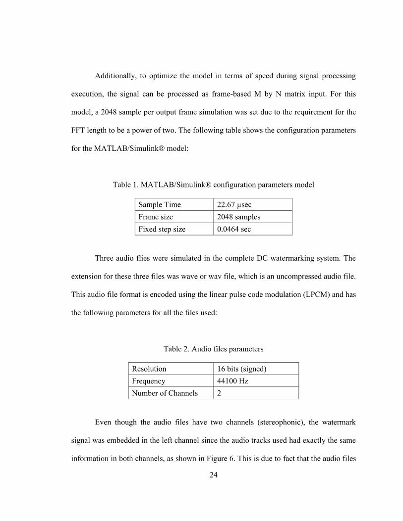
Table 1. MATLAB/Simulink® configuration parameters model
Sample Time 22.67 µsec Frame size 2048 samples Fixed step size 0.0464 sec
Three audio flies were simulated in the complete DC watermarking system. The
extension for these three files was wave or wav file, which is an uncompressed audio file.
This audio file format is encoded using the linear pulse code modulation (LPCM) and has
the following parameters for all the files used:
Table 2. Audio files parameters
Resolution 16 bits (signed) Frequency 44100 Hz Number of Channels 2
Even though the audio files have two channels (stereophonic), the watermark
signal was embedded in the left channel since the audio tracks used had exactly the same
information in both channels, as shown in Figure 6. This is due to fact that the audio files

25
proposed were recorded using an electric guitar, where the output is monophonic or
single channel. However the recording settings were in stereo since most of the
distributed audio files have two channels.
Figure 6. Original waveform of track 1 in stereo
Figure 7 represents the DC watermarking block diagram for the insertion process
using Simulink®. In this model, the host signal is a stereophonic audio file in which the
watermark signal is embedded in both channels. To do so, the signal is divided into left
and right channels. Therefore, the watermark addition and DC removal are performed in
each channel and finally the two channels are combined back together. Due to several
limiting reasons, such as long simulation time and memory usage when implementing the
algorithm in an FPGA board, the DC watermark insertion process was implemented only
in one channel. In the proposed DC watermarking system, the watermark insertion is
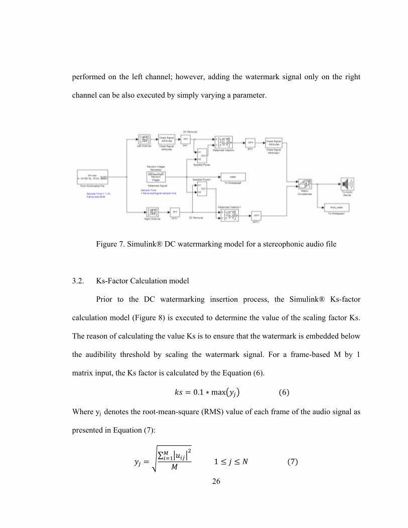
26
performed on the left channel; however, adding the watermark signal only on the right
channel can be also executed by simply varying a parameter.
Figure 7. Simulink® DC watermarking model for a stereophonic audio file
3.2. Ks-Factor Calculation model
Prior to the DC watermarking insertion process, the Simulink® Ks-factor
calculation model (Figure 8) is executed to determine the value of the scaling factor Ks.
The reason of calculating the value Ks is to ensure that the watermark is embedded below
the audibility threshold by scaling the watermark signal. For a frame-based M by 1
matrix input, the Ks factor is calculated by the Equation (6).
Where yj denotes the root-mean-square (RMS) value of each frame of the audio signal as
presented in Equation (7):
27
Where M = size of each frame
N = number of frames
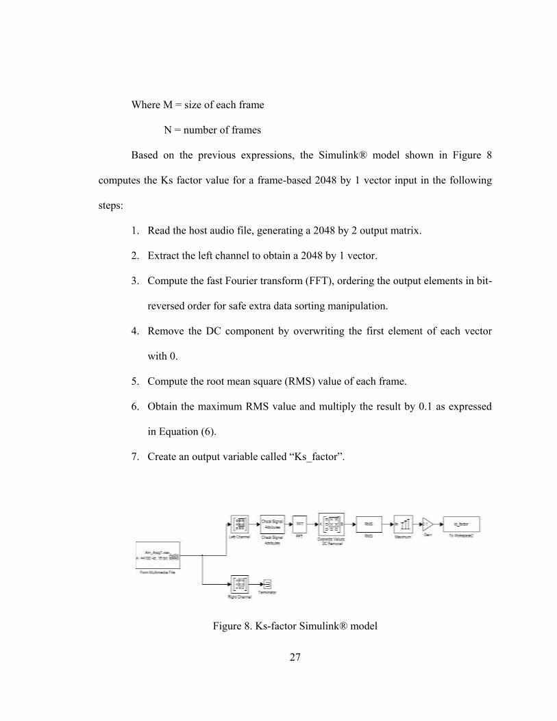
Based on the previous expressions, the Simulink® model shown in Figure 8
computes the Ks factor value for a frame-based 2048 by 1 vector input in the following
steps:
1. Read the host audio file, generating a 2048 by 2 output matrix.
2. Extract the left channel to obtain a 2048 by 1 vector.
3. Compute the fast Fourier transform (FFT), ordering the output elements in bit-
reversed order for safe extra data sorting manipulation.
4. Remove the DC component by overwriting the first element of each vector
with 0.
5. Compute the root mean square (RMS) value of each frame.
6. Obtain the maximum RMS value and multiply the result by 0.1 as expressed
in Equation (6).
7. Create an output variable called “Ks_factor”.
Figure 8. Ks-factor Simulink® model

28
3.3. Watermark Insertion Model
Once the Ks factor of the host audio file has been calculated, the DC watermark
insertion process described in the previous chapter can be performed. Figure 9 represents
the basic DC watermarking block diagram for this process, which was implemented in
Simulink®. Figure 9 shows that the fast Fourier transform has to be computed in order to
perform the power spectral density analysis and watermark addition stages in the
frequency domain. The inverse fast Fourier transform maps the embedded watermark
signal in the time domain, creating the watermarked signal output. As a result, the
performance of the DC watermarking model can be tested by verifying whether or not the
watermark signal is imperceptible to the human auditory system.
Figure 9. Basic DC watermarking insertion model block diagram
OriginalAudio input
Read AA
FFTPSD
Analysis
WatermarkSignal
Pfram
ex Ks
w
WatermarkAddition
W
iFFT
WatermarkedSignal
A’
F(A)
29
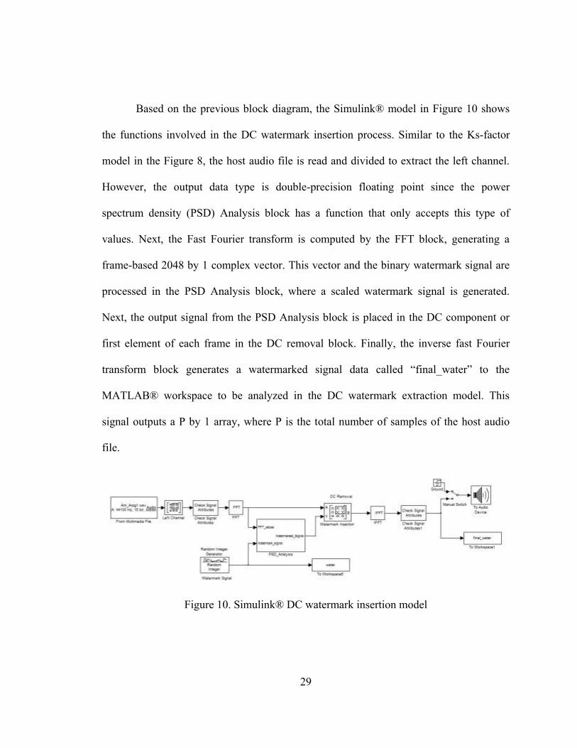
Based on the previous block diagram, the Simulink® model in Figure 10 shows
the functions involved in the DC watermark insertion process. Similar to the Ks-factor
model in the Figure 8, the host audio file is read and divided to extract the left channel.
However, the output data type is double-precision floating point since the power
spectrum density (PSD) Analysis block has a function that only accepts this type of
values. Next, the Fast Fourier transform is computed by the FFT block, generating a
frame-based 2048 by 1 complex vector. This vector and the binary watermark signal are
processed in the PSD Analysis block, where a scaled watermark signal is generated.
Next, the output signal from the PSD Analysis block is placed in the DC component or
first element of each frame in the DC removal block. Finally, the inverse fast Fourier
transform block generates a watermarked signal data called “final_water” to the
MATLAB® workspace to be analyzed in the DC watermark extraction model. This
signal outputs a P by 1 array, where P is the total number of samples of the host audio
file.
Figure 10. Simulink® DC watermark insertion model

30
It is important to mention that the watermark signal is a series of binary random
numbers generated by the Watermark Signal block in the Figure 10. This block generates
a binary double output data type sequence every frame period. Therefore, it is required to
make a rate conversion in order to maintain the same frame size during the simulation.
This can be accomplished by setting the Watermark Signal block sample time as
described in the Equation (8) :
Where, Tf corresponds to the frame period, Ts to the sample period, and M is the frame
size of the host audio signal.
The generated binary watermark signal is also saved in the MATLAB®
workspace in order to be compared with the watermarked signal during the DC
Watermark Extraction model.
3.3.1. Power Spectral Density Analysis
The power spectral density analysis subsystem, shown in Figure 10, contains the
functions that appear in Figure 11. This subsystem performs the scaling of the binary
watermark signal by multiplying the three variables expressed in Equation (9).
31
Where, P corresponds to the Power spectral density of each frame, Ks the scaling factor,
w the binary watermark signal, W the scaled watermark signal, and N is the number of
frames.
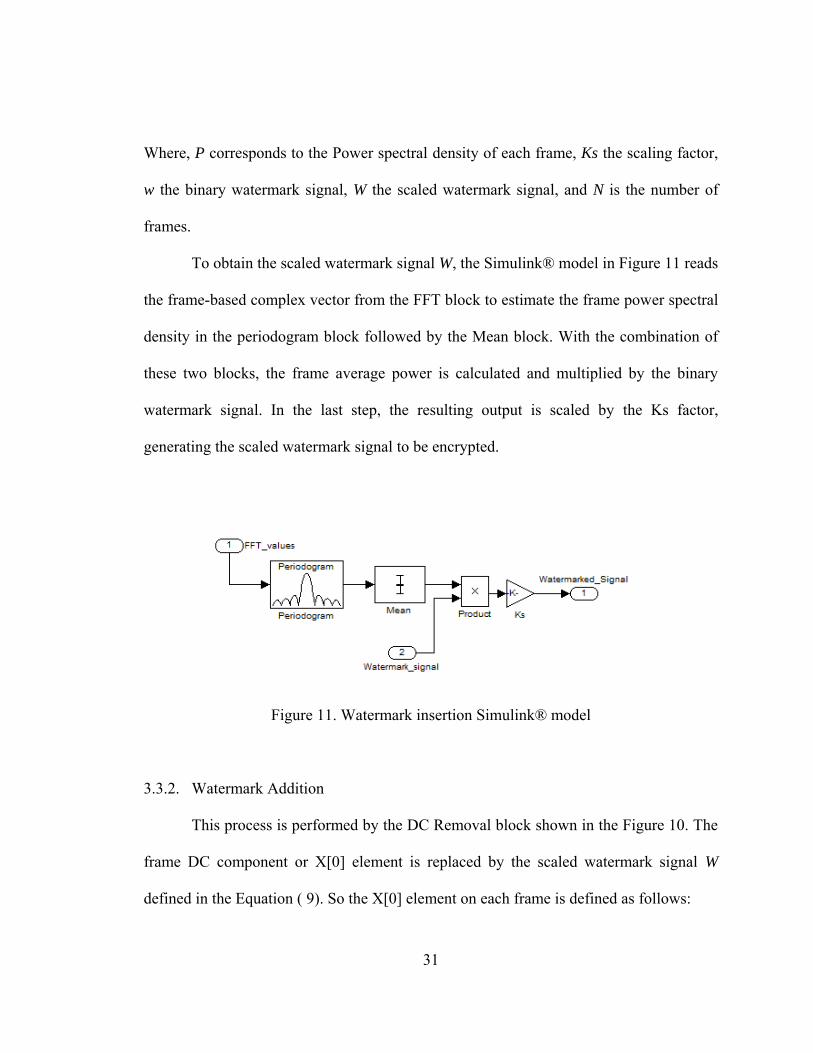
To obtain the scaled watermark signal W, the Simulink® model in Figure 11 reads
the frame-based complex vector from the FFT block to estimate the frame power spectral
density in the periodogram block followed by the Mean block. With the combination of
these two blocks, the frame average power is calculated and multiplied by the binary
watermark signal. In the last step, the resulting output is scaled by the Ks factor,
generating the scaled watermark signal to be encrypted.
Figure 11. Watermark insertion Simulink® model
3.3.2. Watermark Addition
This process is performed by the DC Removal block shown in the Figure 10. The
frame DC component or X[0] element is replaced by the scaled watermark signal W
defined in the Equation ( 9). So the X[0] element on each frame is defined as follows:

32
As mentioned, the watermark embedding process is performed in the frequency
domain; thus, the use of an inverse FFT block will provide the watermarked signal in the
time domain. As a result, the watermarked signal A’ can be expressed as
here A is the original audio signal and W corresponds to the scaled watermark
signal. At the end of this process, the watermarked signal is ready to be tested and
extracted.
3.4. Watermark Extraction System Description
Once the watermark is embedded, the DC watermark insertion model creates a
variable called „final water‟ that represents the watermarked signal A’. This signal is
analyzed in the second model of the complete Simulink® DC watermark system, which
performs the watermark extraction process. The watermark extraction model is described
in the following diagram:
33
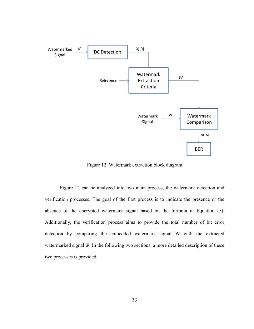
Figure 12. Watermark extraction block diagram
Figure 12 can be analyzed into two main process, the watermark detection and
verification processes. The goal of the first process is to indicate the presence or the
absence of the encrypted watermark signal based on the formula in Equation (5).
Additionally, the verification process aims to provide the total number of bit error
detection by comparing the embedded watermark signal W with the extracted
watermarked signal . In the following two sections, a more detailed description of these
two processes is provided.
WatermarkedSignal
DC DetectionA’
Watermark Extraction
CriteriaReference
Xj[0]
WatermarkComparison
Watermark Signal
w
BER
error

34
3.4.1. Watermark Detection Model
In this process, a similar method used in the DC watermark insertion process is
performed in the watermark detection model (see Figure 13). The watermarked signal is
read, extracting the left channel of the watermarked audio file A’. This is because the
watermark signal W was embedded in the left channel. After that, the FFT block is
performed to analyze the watermarked signal A’ in the frequency domain, where the DC
component is extracted. The extracted DC component is an M x 1 vector whose values
correspond to Equation (10) since the watermark signal W is equal to the extracted
watermark signal .
Figure 13. Watermark detection Simulink® model
As described in Equation (5), the DC component or X[0] element of each frame is
compared to a fixed value, generating an extracted binary watermark signal variable.
This is because the extraction criteria generates a variable . Ideally, this
variable has to be equal to the embedded binary watermark signal w; however, there are
some other factors, like noise, that might alter the information in the embedded

35
watermark signal W. The following watermark verification model is implemented in the
DC Watermark extraction process to confirm that the extracted signal is equal to the
original watermark signal w.
3.4.2. Watermark Verification Model
The Simulink® watermark verification model, as shown in Figure 14, is a
complement of the DC Watermark extraction process since it determines whether or not
the DC watermark insertion model meets the insertion and extraction requirements. The
methodology to verify that assumption is to compare the extracted watermark signal
with the original watermark signal w. The comparison process will generate an M by 1
error vector , where and M is the total number of frames of the audio
signal.
The error variable can be expressed as:
As shown in Equation (11), the error variable assigns the value 1 when the two compared
watermark signals are different; otherwise, a zero is assigned. Another measurement error
variable is the B_error variable that sums the number of errors detected by the error
variable.

36
Then, the B_error variable is expressed as:
Figure 14 - Simulink® watermark verification model
Additionally, the Simulink® model in Figure 14 can also provide more
information about the DC Watermark Simulink® model performance. Such information
is the bit-error rate (BER) that aims to measure the success of the recovery process and
the robustness of the DC Watermarking scheme, as a result.
3.5. Performance and Discussion
In this section, the performance of the DC audio watermarking scheme is tested
and analyzed using the proposed MATLAB/Simulink® model described in this chapter.
To analyze the performance of the model, the fidelity or imperceptibility and
effectiveness properties were evaluated. Three audio files were used to evaluate the
37
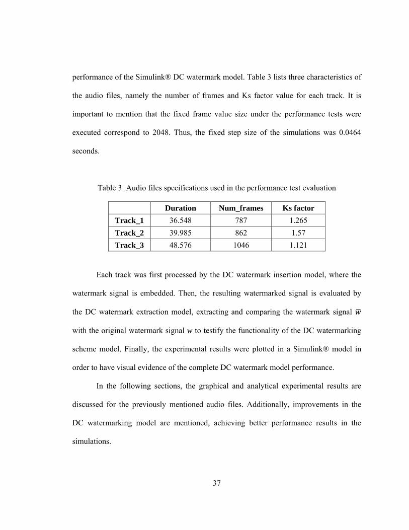
performance of the Simulink® DC watermark model. Table 3 lists three characteristics of
the audio files, namely the number of frames and Ks factor value for each track. It is
important to mention that the fixed frame value size under the performance tests were
executed correspond to 2048. Thus, the fixed step size of the simulations was 0.0464
seconds.
Table 3. Audio files specifications used in the performance test evaluation
Duration Num_frames Ks factor
Track_1 36.548 787 1.265 Track_2 39.985 862 1.57 Track_3 48.576 1046 1.121
Each track was first processed by the DC watermark insertion model, where the
watermark signal is embedded. Then, the resulting watermarked signal is evaluated by
the DC watermark extraction model, extracting and comparing the watermark signal
with the original watermark signal w to testify the functionality of the DC watermarking
scheme model. Finally, the experimental results were plotted in a Simulink® model in
order to have visual evidence of the complete DC watermark model performance.
In the following sections, the graphical and analytical experimental results are
discussed for the previously mentioned audio files. Additionally, improvements in the
DC watermarking model are mentioned, achieving better performance results in the
simulations.

38
3.5.1. Host Audio Signal and Watermarked Signal Comparison
After performing the Simulink® DC watermark model simulation test, a
Simulink® model plotted the experimental results. This useful feature provides a visual
and clear understanding of the model‟s performance. In Figure 15, the resulting
simulation waveforms for Track 1 are displayed. Listed from top to bottom, the original
audio file A (subplot A), the watermarked audio file A’(subplot B), the difference
between A and A’ (subplot C), and the error-variable (subplot D) waveforms are
displayed.
Figure 15. Track1 DC watermarking resulting simulation waveforms
39
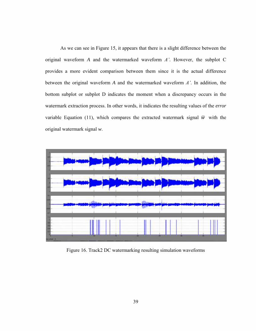
As we can see in Figure 15, it appears that there is a slight difference between the
original waveform A and the watermarked waveform A’. However, the subplot C
provides a more evident comparison between them since it is the actual difference
between the original waveform A and the watermarked waveform A’. In addition, the
bottom subplot or subplot D indicates the moment when a discrepancy occurs in the
watermark extraction process. In other words, it indicates the resulting values of the error
variable Equation (11), which compares the extracted watermark signal with the
original watermark signal w.
Figure 16. Track2 DC watermarking resulting simulation waveforms

40
Figure 17. Track3 DC watermarking resulting simulation waveforms
Figures 16 and 17 display the resulting simulation waveforms for Tracks 2 and 3,
repectively. Conmparing the three plots, we can see that Tracks 1 and 2 present
prolonged peaks in some regions indicated in their respective subplot C. On the other
hand, Track 3 seems to present more incorect extracted bits than the other tracks.
In order to provide more quantitative information than graphical model
performance representations, we can interpret the resulting values using mathematical
equations to measure the impact that the DC watermarking scheme has on the host audio
signal. As mentioned in the Chapter 2, the fidelity property refers to the similarity
between the host audio signal and the watermarked signal. In other words, the
watermarked signal should maintain the sound quality of the original audio signal. The
fidelity performance evaluation can be measured using objective and subjective

41
degradations [19]. The subjective degradation refers to the perceptual test or listening
test, where trained listeners grade the quality of the watermarked signal based on an
impairment scale according to [1], [19], and [22]. On the other hand, the objective
degradation measures the quality of the watermarked signal quantitatively. Using
statistical metrics, the objective degradation can be determined.
To measure the resulting degradation of the DC watermarking scheme, three
common objective degradation metrics were used [1]. These metrics are the Maximum
Difference (MD), Average Absolute Difference (AD), and Mean Square Error (MSE),
which are defined as follows:
Where, A corresponds to the original audio signal, A’ to the watermarked signal, and N
the nth sample of the watermarked signal A.
A MATLAB® code computes the MD, AD, and MSE formulas using the original
audio signal A and the watermarked signal A’ from the Simulink® DC watermarking
model simulations as inputs. The results are listed in Table 4 for the three proposed audio

42
files. In addition, it also includes the number of bit errors obtained during the watermark
verification model (Figure 14) defined by the Bit_error variable Equation (12).
Table 4. Common effectiveness and objective degradation metrics
Num_error MD AD MSE
Track_1 34 0.1442 0.0156 7.56e-4 Track_2 42 0.1044 0.0151 5.70e-4 Track_3 60 0.047 0.0127 2.65e-4
From Table 4, the assumptions obtained from the three DC Watermarking
resulting simulation waveforms are confirmed (see Figures 15, 16, and 17). In terms of
watermark system effectiveness, the Watermark extraction model (Figure 12) was unable
to recover the complete watermark signal. As listed in Table 4 and displayed in Figure
17, Track 3 shows more bit errors detected than the other tracks. However in relation to
fidelity, the same Track 3 has less degradation than the rest.
Even though the results shown in Table 4 seem to be acceptable, these results
provide a quantitative metric of the impact or difference between the watermarked and
the original signals and do not reflect the exact perceived noise [1] and [19]. Therefore,
informal subjective degradation tests or listening tests were performed. As a result,
whereas the watermarked Tracks 1 and 2 include perceptible and annoying noise, Track 3
poses slightly annoying noise. This conclusion can be visually confirmed by analyzing
Figures 15, 16, and 17, where the tracks 1 and 2 have prolonged peaks in some portions
in their respective subplots C.

43
3.5.2. Bit Error Rate and SNR Analysis
In addition to the MD, AD, and MSE formulas (Equations 13, 14, and 15) to
measure the fidelity of the DC watermark model, the signal-to-noise ratio (SNR) or
signal-to-watermark ratio (SWR) was implemented. This difference distortion metric is
the most representative metric in terms of embedding watermark distortion used in the
audio watermarking literature [1], [4], [19], and [22]. The SNR is defined as follows:
Where, A corresponds to original audio signal, A’ to the watermarked signal, and N is the
total number of samples of the watermark signal A. The SNR is measured in decibels
(dB) using the above expression.
For the watermark recovery performance, another frequent effectiveness metric
applied in the audio watermarking literature is the Bit-Error Rate (BER) [1], [4], [19],
and [22]. The BER determines the percent number of incorrect extracted bits by
comparing the embedded watermark signal w with the extracted watermark signal , and
it is given by the following expression:
44
Where, is the embedded watermark signal, corresponds to the extracted
watermark signal, and N the length of the embedded watermark w. The BER is also used
to measure the robustness of the audio watermark after experiencing any signal
processing attack.
A MATLAB based code was executed to compute the SNR variable, whereas the
BER values were obtained using the B_error variable (Equation 12) from the Watermark
Verification Model and divided by the number of samples of the same set of audio tracks
listed in Table 3. The resulting simulation values are mentioned in Table 5. While Track
3 poses less embedded distortion than the other tracks, it contains more incorrect
extracted watermark bits than the rest.
Table 5. Experimental BER and SNR values
BER [%] SNR [dB]
Track_1 4.32 33.44 Track_2 4.87 36.89 Track_3 5.73 42.50
In order to improve the fidelity and effectiveness performances of the DC
watermark model, a deeper SNR and BER analysis was performed. The goal of the first
experimental test was to find the impact or correlation between the Ks factor and the

45
SNR variable. The value of Ks factor is closely related to the noise the embedded
watermark signal can add into the host audio file. A MATLAB®-based program was
executed, where the SNR was computed for 100 different Ks factor values as shown in
the following expression, Equation (18). Based on the embedded watermark Equation (9)
and Equation (18), there will be 100 different watermark signals W for each Ks factor
value.
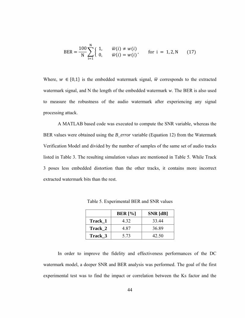
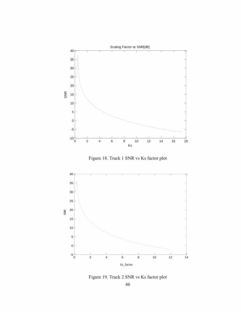
Figures 18 and 19 represent the relationship between SNR and the Ks factor for
Tracks 1 and 2, respectively. From these figures, it can be concluded that as the Ks factor
increases, the signal-to-noise ratio SNR decreases. Thus, the embedded watermark signal
will add noise into the host signal as Ks increases.
46
Figure 18. Track 1 SNR vs Ks factor plot
Figure 19. Track 2 SNR vs Ks factor plot
0 2 4 6 8 10 12 14 16 18-10
-5
0
5
10
15
20
25
30
35
40
Ks
SN
R
Scaling Factor vs SNR[dB]
0 2 4 6 8 10 12 14-5
0
5
10
15
20
25
30
35
40
SNR
Ks_factor
47
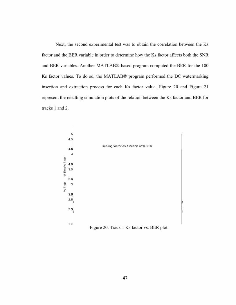
Next, the second experimental test was to obtain the correlation between the Ks
factor and the BER variable in order to determine how the Ks factor affects both the SNR
and BER variables. Another MATLAB®-based program computed the BER for the 100
Ks factor values. To do so, the MATLAB® program performed the DC watermarking
insertion and extraction process for each Ks factor value. Figure 20 and Figure 21
represent the resulting simulation plots of the relation between the Ks factor and BER for
tracks 1 and 2.
Figure 20. Track 1 Ks factor vs. BER plot
0 2 4 6 8 10 12 142.5
3
3.5
4
4.5
5
scaling factor
% E
rror
scaling factor as function of %BER
0 2 4 6 8 10 12 142.5
3
3.5
4
4.5
5
scaling factor
% E
rror
scaling factor as function of %BER
0 2 4 6 8 10 12 142.5
3
3.5
4
4.5
5
scaling factor
% E
rror
scaling factor as function of %BER

48
Figure 21. Track 2 Ks factor vs. BER plot
According to the experimental results provided in the two previous plots, it seems
that the BER is independent on the Ks factor since it remains constant for every Ks
values. Based on this assumption, it can be concluded that the noise or distortion added
by any Ks factor value in the embedded watermark signal W ( Equation 9) will not affect
the resulting BER value for the DC watermark model. To confirm this conclusion,
another experimental test was performed. In this third test, the BER was computed for
100 different Ks factor and embedded binary watermark signal w values, modifying the
two possible variables that can produce a different watermark signal W as defined in the
Equation 9.
0 2 4 6 8 10 12 14 163.5
4
4.5
5
5.5
6
X: 11.68
Y: 4.886
scaling factor
% E
rror
scaling factor as function of %BER

49
Figure 22 provides the experimental results for this test, where the top subplot
shows the resulting BER values for different Ks factor values and the second subplot
displays the number of ones in the binary watermark signal w.
`
Figure 22. BER for different Ks factor and watermark signals plot
From Figure 22, it is clear that for different Ks factor and binary watermark signal
w values, the range of the resulting BER values is approximately between 3.5% and 6%.
Therefore, the BER cannot be improved by altering the embedded watermark signal W
variables in the proposed DC watermark model.
0 2 4 6 8 10 12 14 163
4
5
6
7
scaling factor
BE
R
Ks scaling factor as function of BER
0 2 4 6 8 10 12 14 16350
400
450
500
scaling factor
# o
f oones
Ks scaling factor as function of BER
50
3.5.3. Watermark System Improvement
Based on the conclusions from the experimental tests presented in the previous
section, it can be concluded that the resulting BER values are independent of the
embedded watermark signal. We now should focus on the DC watermark detection
model since the BER evaluates the watermark recovery performance. The only variable
that can be modified in this process is the value defined in Equation 5. However, after
altering some possible values, the embedded watermark signal was never 100%
recovered.
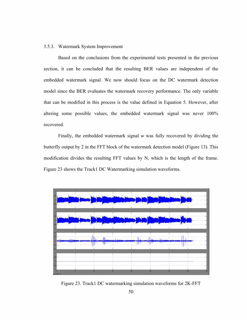
Finally, the embedded watermark signal w was fully recovered by dividing the
butterfly output by 2 in the FFT block of the watermark detection model (Figure 13). This
modification divides the resulting FFT values by N, which is the length of the frame.
Figure 23 shows the Track1 DC Watermarking simulation waveforms.
Figure 23. Track1 DC watermarking simulation waveforms for 2K-FFT

51
From the previous figure, it is notable that the embedded watermark signal w is
totally recovered since the resulting error variable value is zero. Thus, the BER value is
also zero. The same statement can be applied for the other two tracks, where the BER
was also zero. Even though the BER variable was successfully minimized into the ideal
value, the resulting SNR values for the proposed tracks remain unaltered. This can be
visually proved by comparing the watermark difference section or subplot C between
Figure 15 and Figure 23.
3.6. 1K-FFT-Length MATLAB/Simulink® DC Watermarking Model
A second DC watermarking model using Simulink® was developed, with a FFT
length value of 1024. This means that a 1K samples per frame simulation was executed,
so the fixed step time value has changed to 0.0232 seconds. The DC watermarking
insertion and extraction algorithms shown in Figure 9 and Figure 12 were implemented
with the new 1024 frame size variation. In addition, the same set of tracks used in the
previous DC Watermarking performance tests were utilized for this alternative
Simulink® model. The advantage of designing and simulating a second DC
Watermarking model is that more experimental results can offer a better overview of the
proposed audio watermarking scheme. The parameters and simulation results are
provided for this second DC watermarking model are provided in the following section.

52
3.6.1. System Parameters
As mentioned, the new proposed Simulink® DC watermarking model has a frame
size of 1024 samples per frame since the FFT length must be a power of two in order to
obtain accurate FFT resulting values in the simulations. Based on this condition, the first
proposed value corresponded to the result of 2n where n has a value of 11, whereas the
second frame size value is the resulting value when n is equal to 10. In Table 6, the
second configuration parameters are shown for a 1024 frame size simulation.
Table 6. MATLAB/Simulink® configuration parameters for 1K Frame Size
Sample Time 22.67 µsec Frame size 1024 samples Fixed step size 0.0232 sec
Table 6 provides the number of frames and Ks factor values for the same set of
tracks. Each Ks factor was also computed following the algorithm and Simulink® model
described in the Ks-factor calculation model section.
Table 7. Audio files specifications for 1K
Num_frames Ks factor
Track_1 1573 1.055 Track_2 1759 1.222 Track_3 2091 0.985
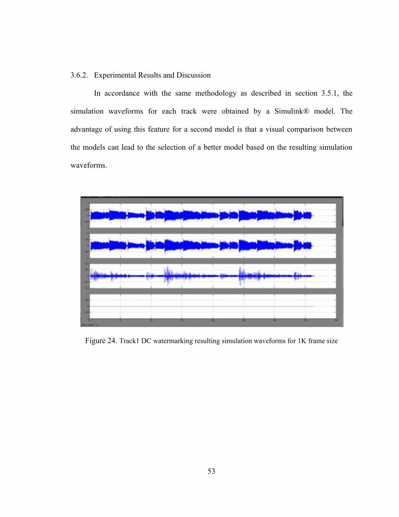
53
3.6.2. Experimental Results and Discussion
In accordance with the same methodology as described in section 3.5.1, the
simulation waveforms for each track were obtained by a Simulink® model. The
advantage of using this feature for a second model is that a visual comparison between
the models can lead to the selection of a better model based on the resulting simulation
waveforms.
Figure 24. Track1 DC watermarking resulting simulation waveforms for 1K frame size

54
Figure 25. Track2 DC watermarking resulting simulation waveforms for 1K frame size
Figure 26. Track3 DC watermarking resulting simulation waveforms for 1K frame size
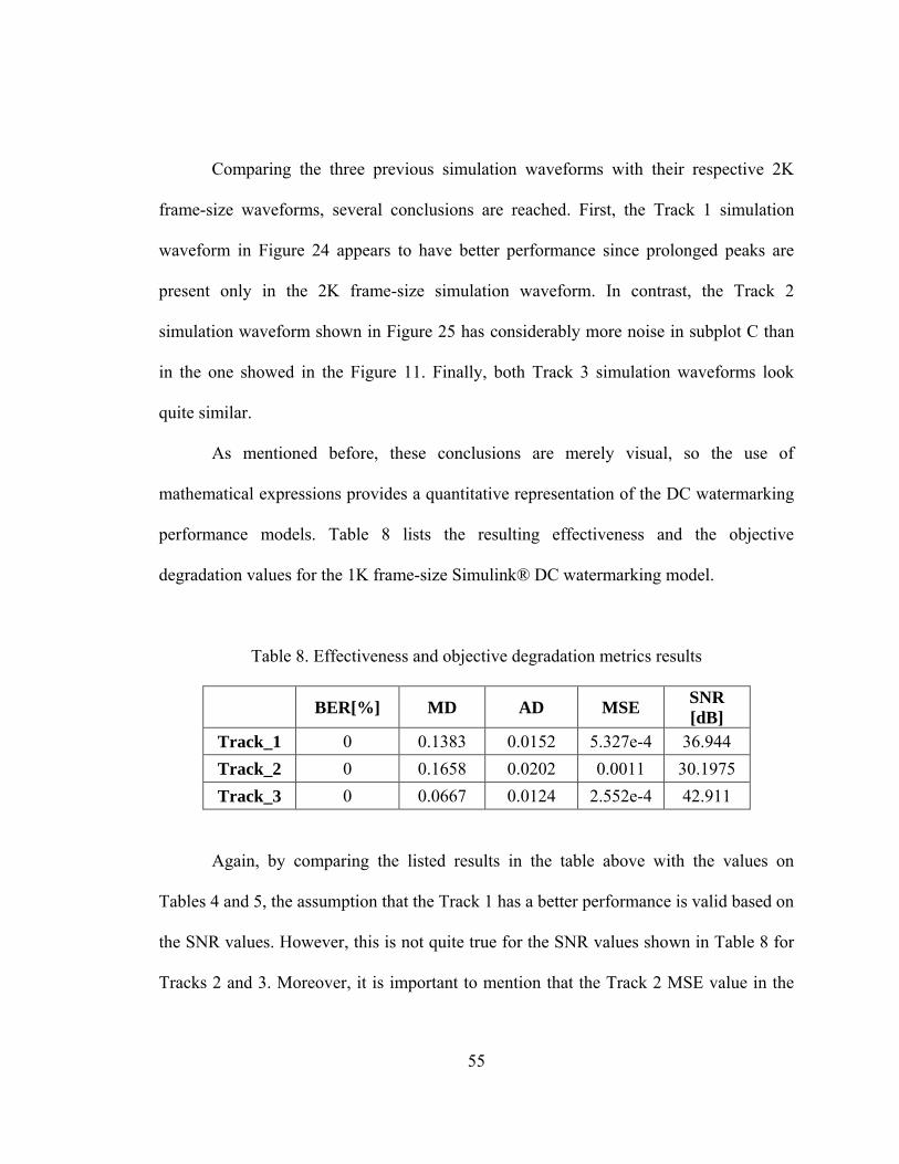
55
Comparing the three previous simulation waveforms with their respective 2K
frame-size waveforms, several conclusions are reached. First, the Track 1 simulation
waveform in Figure 24 appears to have better performance since prolonged peaks are
present only in the 2K frame-size simulation waveform. In contrast, the Track 2
simulation waveform shown in Figure 25 has considerably more noise in subplot C than
in the one showed in the Figure 11. Finally, both Track 3 simulation waveforms look
quite similar.
As mentioned before, these conclusions are merely visual, so the use of
mathematical expressions provides a quantitative representation of the DC watermarking
performance models. Table 8 lists the resulting effectiveness and the objective
degradation values for the 1K frame-size Simulink® DC watermarking model.
Table 8. Effectiveness and objective degradation metrics results
BER[%] MD AD MSE SNR
[dB]
Track_1 0 0.1383 0.0152 5.327e-4 36.944 Track_2 0 0.1658 0.0202 0.0011 30.1975 Track_3 0 0.0667 0.0124 2.552e-4 42.911
Again, by comparing the listed results in the table above with the values on
Tables 4 and 5, the assumption that the Track 1 has a better performance is valid based on
the SNR values. However, this is not quite true for the SNR values shown in Table 8 for
Tracks 2 and 3. Moreover, it is important to mention that the Track 2 MSE value in the

56
same table is almost two times more than the resulting MSE value on Table 4. Looking at
Figure 25, the resulting simulations show noise in many regions.
Additionally, an informal subjective degradation test was performed for this
second Simulink® DC watermarking model. The listening test results indicate that Track
1 has a better fidelity performance even though Track 3 has the biggest SNR value. This
confirms that the actual perceptual noise is not always represented by the resulting SNR
value.

57
CHAPTER 4
DSP BUILDER AND MATLAB/SIMULINK® MODEL IMPLEMENTATION
The purpose of this chapter is to present the implementation of the watermark
insertion models described in Chapter 3 using an Altera® Cyclone II [8] device. The
main reason of implementing the watermark insertion model in a field-programmable
gate array (FPGA) chip is that superior signal processing performance can be achieved
[7] and [23]. In order to achieve this goal, different models were designed, simulated,
implemented, and compared with the existing MATLAB/Simulink® [9] programming
language watermarking model. The coverage of the FPGA device implementation of
audio watermarking is discussed in three sections. The first section introduces the FPGA
and digital signal processing (DSP) builder features and system level design flow using
DSP builder in the watermark model. In the next two sections, two software-hardware
models are described as well as performance and comparison tests results.
4.1. Hardware Implementation
In addition to the already mentioned reasons of implementing the audio
watermarking model on a field-programmable gate array FPGA device, most of the
digital signal processing applications require specific DSP processors to satisfy system
requirements. However, DSP processors have fixed hardware architecture, making the
hardware implementation inefficient in terms of performance and cost.

58
As an alternative solution for this problem, the use of FPGAs can provide better
system performance and lower costs in most DSP applications [7]. This is achieved due
to the fact that the FPGA‟s hardware architecture can be reconfigurable, offering
customized DSP applications. In other words, the designers can develop a complete
system using an FPGA with customized architecture, bus structure, memory, and
hardware accelerator blocks. This advantage makes FPGAs more suitable for many DSP
applications such as the direct current (DC) audio watermarking system described in this
project.
An Altera® Cyclone II FPGA device was utilized to implement the DC audio
watermarking system. Moreover, Altera® offers a powerful DSP design tool named
MegaCore® [8] functions. This DSP tool covers many critical functions such as filters,
transforms, and signal generation functions, which are used in most DSP designs. The
benefit of using MegaCore® functions is that DSP systems can reach efficient hardware
configurations since they can be parameterized [6] and [7]. The use of the fast Fourier
transform (FFT) MegaCore® function was implemented in this project because the fast
Fourier transform is essential to the proposed DC audio watermarking scheme.
MegaCore® functions can be implemented in a hardware description language (HDL)
like VHDL. However, Altera® also provides a powerful tool called DSP Builder, where
the hardware implementation is represented in an algorithm development environment.
For this project, the proposed DC audio Watermarking scheme was implemented using
Simulink® and the DSP Builder tool in order to implement the watermarking model in an
FPGA device.

59
4.1.1. FPGA and DSP Builder Features
In the previous section, the advantages of implementing a DSP system in an
FPGA device over specialized DSP processors were mentioned. The most important
advantage is the flexibility of customizing the hardware architecture in the FPGA rather
than implement the DSP system in a fixed hardware architecture processor. In order to
satisfy this feature, FPGA architecture includes several embedded components which are
able to fit any DSP system to the FPGA device following the designer‟s hardware
specification. The Altera® Cyclone II FPGA device used in this project has the following
features [7]:
Embedded memory
Embedded DSP blocks
External memory interfaces
Embedded multipliers
Advanced I/0 standard support
Global clock network
Logic elements & logic array blocks
All these elements are configurable in order to satisfy the DSP system
functionality. For instance, the embedded DSP and memory blocks are widely used to
parameterize and program the MegaCore® functions such as the FFT and finite impulse
response (FIR) blocks. There are several ways to configure these DSP functions that
Altera® offers to the designer. One method can be using a HDL language like VHDL in
the Quartus II® [8] design software form Altera®. However, the designer must have a

60
broad HDL language knowledge to effectively utilize this approach and it can become
fairly complicated when designing complex DSP systems. An alternative configuring
DSP function solution provided by Altera® is the use of the DSP Builder tool. This
powerful tool can configure and program any MegaCore® function in an algorithm
development software such as MATLAB® and Simulink® [7]. As a result, any DSP
function like the FFT MegaCore® function can be configured and built in the
MATLAB®/Simulink® environment using the Altera® DSP Builder tool. Some of the
most important DSP Builder features are [10] and [24]:
MATLAB® and Simulink® software compatibility with the Quartus II®
software
Combining existing MATLAB® and/or Simulink® programs with the
Altera® DSP Builder tool
Automated Quartus II® compilation process for DSP designs in
Simulink®
FPGA hardware co-simulation with Hardware in the Loop (HIL) using
Simulink®
MegaCore® function instantiation feature
Importing VHDL or Verilog HDL files into Simulink®
The combination of these DSP Builder features makes any DSP model
implementation in an FPGA device possible with minimal HDL knowledge from the
designer. For example, when implementing the DC audio watermarking in an FPGA
device, it was necessary to import a VHDL file for the FFT MegaCore® controller.
61
4.1.2. FFT MegaCore® Function Description
This DSP function performs the FFT function with very high performance. This
MegaCore® function is parameterized and generated using the DSP Builder tool,
improving the DSP model in terms of performance, flexibility, time and memory
consumption. The FFT MegaCore® function is completely compatible in most of the
Altera® FPGA device families like the used Cyclone® II FPGA device. The designer can
implement this DSP function to perform both the FFT and inverse FFT functions using a
block-floating-point (BFP) architecture to guarantee the total input data width during the
FFT calculation values process [25]. Additionally, this architecture also provides a better
SNR performance when implementing the DSP in a FPGA chip.
Like all MegaCore® functions, the FFT function is parameterized in order to
obtain high FPGA implementation performance. This block has two engine architectures
that define the number of parallel engines which can optimize either the time or size of
the transform. Additionally, it has streaming, burst and buffered burst options to define
the I/O data flow during the transform. The main difference among these operational
options is the resulting latency in the FFT process.
For this project, the streaming data flow option was implemented where the FFT
function control signals are generated by a custom built controller. To allow the correct
data transfer in the FFT function, the sink_valid and sink_ready signals are asserted as
shown in Figure 27. Then, the controller sends the start of packet (SOP) and end of
packet (EOP) signals, indicating the start and end of the FFT frame respectively. Next,
the FFT function block computes the incoming values and asserts the source_valid signal

62
indicating available output data. In the same way, the FFT block outputs the source_SOP
and end source_EOP signals to specify the start and end of the output FFT frame, as
shown in Figure 27.
Figure 27. FFT function streaming data flow
Analyzing Figure 27, it is notable that there is latency of almost two input frames
to perform the Fourier transform. During each FFT calculation value stage, the input is
scaled in order to provide high precision in the resulting values.
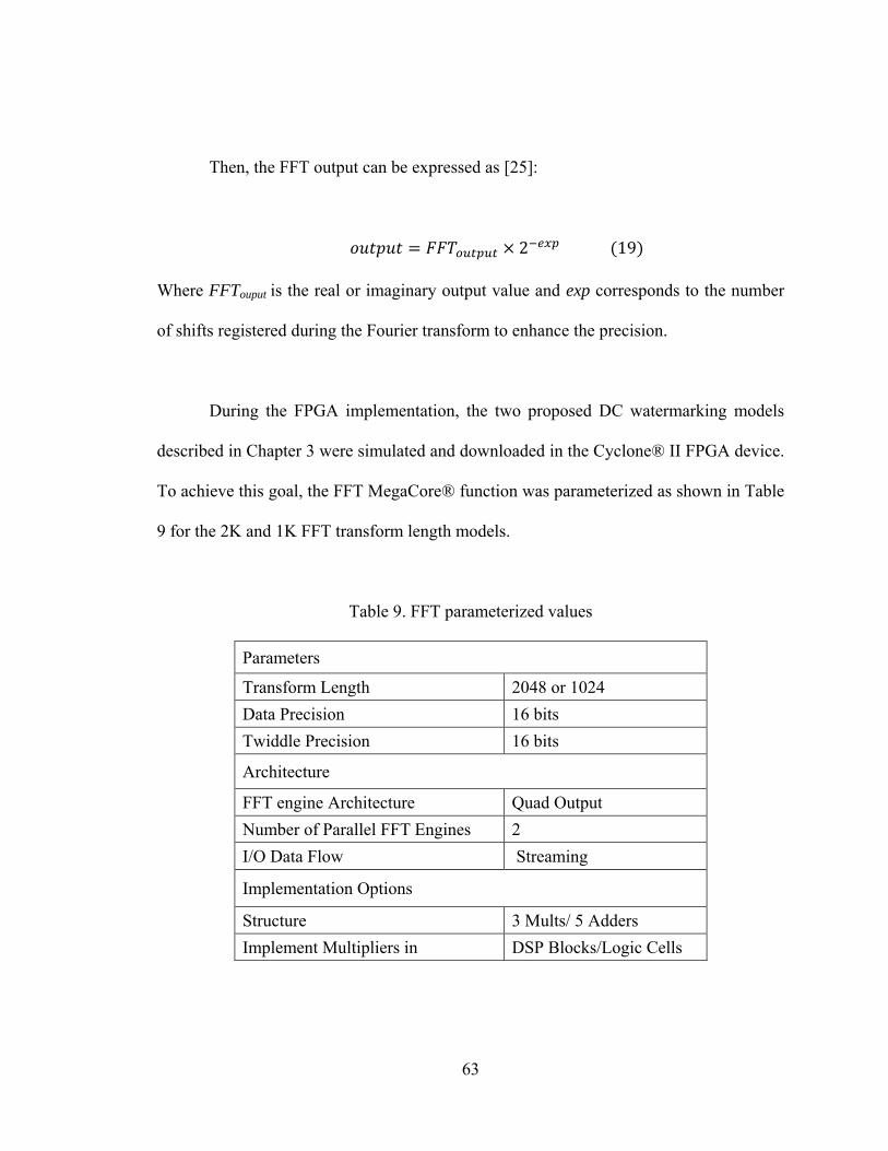
63
Then, the FFT output can be expressed as [25]:
Where FFTouput is the real or imaginary output value and exp corresponds to the number
of shifts registered during the Fourier transform to enhance the precision.
During the FPGA implementation, the two proposed DC watermarking models
described in Chapter 3 were simulated and downloaded in the Cyclone® II FPGA device.
To achieve this goal, the FFT MegaCore® function was parameterized as shown in Table
9 for the 2K and 1K FFT transform length models.
Table 9. FFT parameterized values
Parameters
Transform Length 2048 or 1024 Data Precision 16 bits Twiddle Precision 16 bits
Architecture
FFT engine Architecture Quad Output Number of Parallel FFT Engines 2 I/O Data Flow Streaming
Implementation Options
Structure 3 Mults/ 5 Adders Implement Multipliers in DSP Blocks/Logic Cells
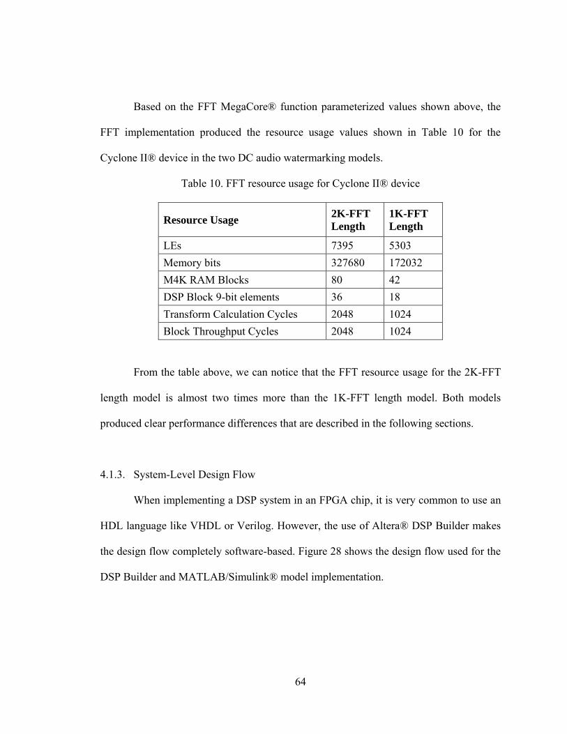
64
Based on the FFT MegaCore® function parameterized values shown above, the
FFT implementation produced the resource usage values shown in Table 10 for the
Cyclone II® device in the two DC audio watermarking models.
Table 10. FFT resource usage for Cyclone II® device
Resource Usage 2K-FFT
Length
1K-FFT
Length
LEs 7395 5303 Memory bits 327680 172032 M4K RAM Blocks 80 42 DSP Block 9-bit elements 36 18 Transform Calculation Cycles 2048 1024 Block Throughput Cycles 2048 1024
From the table above, we can notice that the FFT resource usage for the 2K-FFT
length model is almost two times more than the 1K-FFT length model. Both models
produced clear performance differences that are described in the following sections.
4.1.3. System-Level Design Flow
When implementing a DSP system in an FPGA chip, it is very common to use an
HDL language like VHDL or Verilog. However, the use of Altera® DSP Builder makes
the design flow completely software-based. Figure 28 shows the design flow used for the
DSP Builder and MATLAB/Simulink® model implementation.

65
Figure 28 DC audio watermarking design flow [7] and [24]
The system-level design flow shown in Figure 28 makes the DSP system
hardware implementation simplified and user-friendly since the designer can implement a
specific DSP model using a complete software-based design flow. Based on this design
flow, the DSP model was designed using MATLAB® and Simulink®. Next, by
implementing the Altera® DSP blocks, such as the FFT MegaCore® function and
counters, the final model can be synthesized to generate the VHDL files. These files are
automatically generated within Simulink® by the Signal compiler, where a Quartus® II
project for the resulting model is also created. From this point, a Simulink® model
simulation can be executed to analyze the behavior of the DSP system in the FPGA
device. Additionally, the model can be also implemented in an FPGA device using the
hardware-in-the-loop (HIL) co-simulation.
MATLAB/Simulink
DSP BuilderSignal Compiler
Simulink Simulation
Quartus II Synthesis
ATOM Netlist
Quartus II Fitter
DSP Libraries
HIL Co-Simulation
Hardware
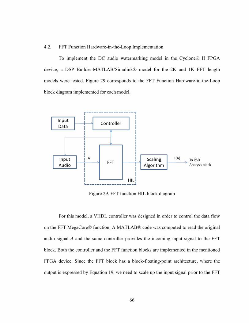
66
4.2. FFT Function Hardware-in-the-Loop Implementation
To implement the DC audio watermarking model in the Cyclone® II FPGA
device, a DSP Builder-MATLAB/Simulink® model for the 2K and 1K FFT length
models were tested. Figure 29 corresponds to the FFT Function Hardware-in-the-Loop
block diagram implemented for each model.
Figure 29. FFT function HIL block diagram
For this model, a VHDL controller was designed in order to control the data flow
on the FFT MegaCore® function. A MATLAB® code was computed to read the original
audio signal A and the same controller provides the incoming input signal to the FFT
block. Both the controller and the FFT function blocks are implemented in the mentioned
FPGA device. Since the FFT block has a block-floating-point architecture, where the
output is expressed by Equation 19, we need to scale up the input signal prior to the FFT
ScalingAlgorithm
InputAudio
FFT
Input Data
Controller
HIL
To PSD Analysis block
F(A)A

67
process and scale the output back by the kn factor as expressed in Equation 20 Otherwise,
a loss of precision in the FFT process would occur.
Where and y is the mth sample of the original audio signal A.
Therefore, the resulting output value for the FFT block is as follow:
Now, the output from the Scaling Algorithm is the actual FFT value of the host
signal A. This signal is processed in the Simulink® model shown in Figure 30 where the
power spectrum density (PSD) analysis and watermarking addition processes are
performed in accordance to the DC audio watermarking scheme.
Figure 30. PSD analysis and watermark addition Simulink® model

68
4.2.1. MATLAB/Simulink and DSP Builder Model Description
Figure 31 displays the actual FFT Function model using MATLAB/Simulink®
and DSP Builder functions. As mentioned, the controller manages the control FFT block
and input audio block signals to guarantee the correct data flow and FFT performance.
For this model, it was necessary to obtain the total number of frames for the host audio
file to indicate when the last input frame occurs. Therefore, the controller stops sending
real values to the FFT block. The resulting total number of frames was computed by a
MATLAB® code which depends on the frame size. In this case, the 1K and 2K frame
sizes were implemented.
Figure 31. MATLAB/Simulink® and DSP Builder model
After compiling the Simulink® model, a VHDL file is created by the Signal
compiler block. As a result, this model can be also simulated using the Quartus® II
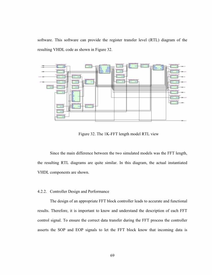
69
software. This software can provide the register transfer level (RTL) diagram of the
resulting VHDL code as shown in Figure 32.
Figure 32. The 1K-FFT length model RTL view
Since the main difference between the two simulated models was the FFT length,
the resulting RTL diagrams are quite similar. In this diagram, the actual instantiated
VHDL components are shown.
4.2.2. Controller Design and Performance
The design of an appropriate FFT block controller leads to accurate and functional
results. Therefore, it is important to know and understand the description of each FFT
control signal. To ensure the correct data transfer during the FFT process the controller
asserts the SOP and EOP signals to let the FFT block know that incoming data is

70
available. The period for the SOP and EOP depends of the parameterized frame size or
transform length.
Figure 33 shows a brief example of the controller performance. In this example,
five input frames with a sample time of 1/44100 seconds are simulated in Simulink®.
From the same figure, it can be noted that the input signal is sent to the FFT block as long
as the valid control signal is asserted. However, this control signal depends on the
specified total number of frames obtained by a MATLAB® code.
Figure 33. The controller performance simulation
The controller is completely developed using the Quartus® II software since is
VHDL code. Subsequently, the file is compiled and imported to Simulink® as a new
DSP block. The clock used in the controller is the Simulink® sample time clock. Once
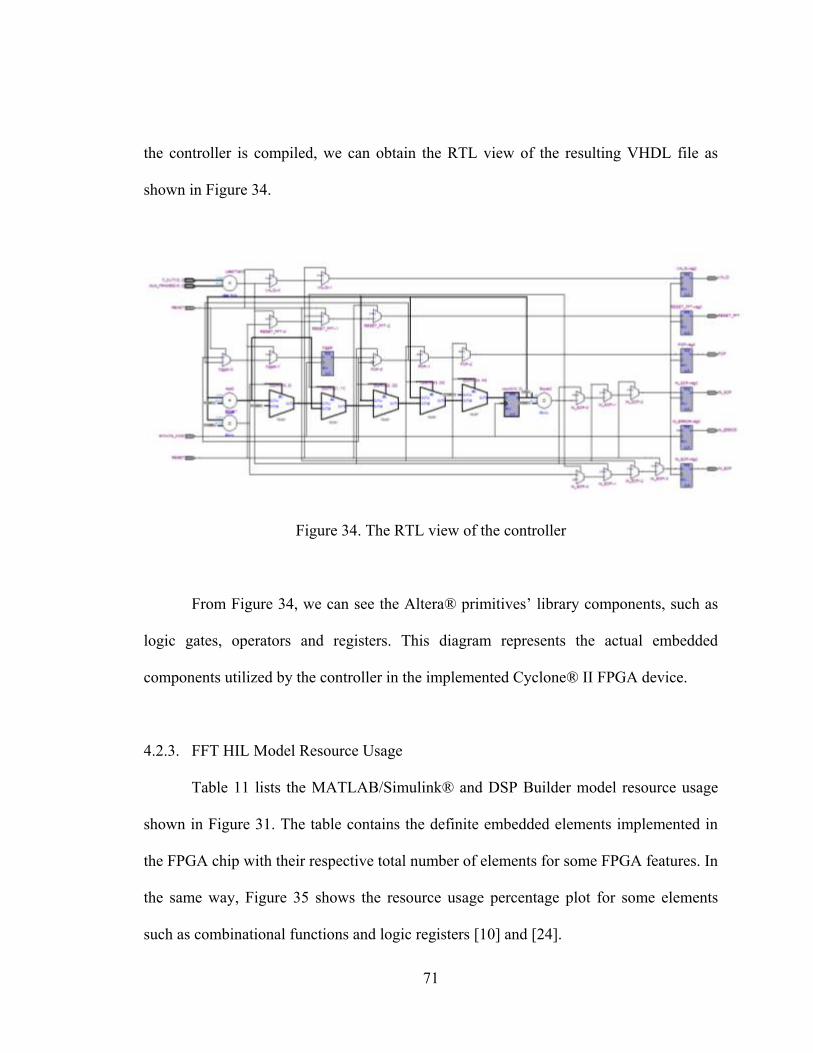
71
the controller is compiled, we can obtain the RTL view of the resulting VHDL file as
shown in Figure 34.
Figure 34. The RTL view of the controller
From Figure 34, we can see the Altera® primitives‟ library components, such as
logic gates, operators and registers. This diagram represents the actual embedded
components utilized by the controller in the implemented Cyclone® II FPGA device.
4.2.3. FFT HIL Model Resource Usage
Table 11 lists the MATLAB/Simulink® and DSP Builder model resource usage
shown in Figure 31. The table contains the definite embedded elements implemented in
the FPGA chip with their respective total number of elements for some FPGA features. In
the same way, Figure 35 shows the resource usage percentage plot for some elements
such as combinational functions and logic registers [10] and [24].

72
Table 11. 2K-FFT HIL model resource usage
Total logic elements 7.783/33.216 Total combinational functions 6.368/33.216 Dedicated logic registers 6.785/33.216 Total registers 6785 Total memory bits 311.793/483.840 Embedded Multiplier 9-bit elements 36/70 Total PLLs 0/4
Figure 35. The 2K-FFT HIL model resource usage percentage plot
From Figure 35, it can be concluded that the 2K-FFT HIL model consumes 64%
of the available memory bits for the Cyclone® II FPGA device. Most of this
consumption is due to the FFT function block. However, after simulating the final model,
very acceptable outcomes were obtained from this particular model.
19% 20 % 64 % 51 %
0%
10%
20%
30%
40%
50%
60%
70%
Total combinational
functions
Dedicated logic registers
Total memory bits
Embedded Multiplier 9-bit
elements

73
Similarly, Table 12 lists the resource usage for the 1K-FFT HIL model with its
respective percentage plot (see Figure 36).
Table 12. 1K-FFT HIL model resource usage
Total logic elements 5.560/33.216 Total combinational functions 4.321/33.216 Dedicated logic registers 4.888/33.216 Total registers 4888 Total memory bits 156.140/483.840 Embedded Multiplier 9-bit elements 18/70 Total PLLs 0/4
Figure 36. The 1K-FFT HIL Model resource usage percentage plot
Comparing the resulting tables and figures, it is evident that the FFT function
Hardware-in-the-Loop model for 1024 FFT transformation length uses fewer resources
than the 2048 FFT transformation length. It is important to mention that one of the
13 % 15 % 32 % 26 %
0%
5%
10%
15%
20%
25%
30%
35%
Total combinational
functions
Dedicated logic registers
Total memory bits
Embedded Multiplier 9-bit
elements

74
embedded elements that reduces the cost when implementing a DSP system in a FPGA
device is the total memory bits. Whereas the 2K-FFT HIL model requires a total
percentage of 64% to perform the FFT function, the 1K-FFT HIL model uses only half of
the total capacity.
Even though two different FFT Hardware-in-the-loop models were co-simulated
using Simulink®, both had a simulation rate of 1.80 minutes to process 1 second of
sound. However the resulting simulation waveforms and performance differ as described
in the next section. The same holds for the MATLAB/Simulink®-based audio
watermarking comparison models.
4.2.4. HIL DC Watermarking Model Testing and MATLAB/Simulink® Model
Comparison
For the FFT Function HIL model shown in Figure 29, two different models were
implemented in a Cyclone® II FPGA device. The only difference between them is that
the FFT transformation length is equal to 2048 for one model and 1024 for the other.
Based on the same figure, it is noted that the most important implemented DSP function
block is the FFT MegaCore® function, so it is necessary to guarantee the right
performance of this block in order to obtain accurate and better performance results than
the Simulink®-based DC watermarking models described in Chapter 3.
The first performance test was to compare the resulting FFT values from the
FPGA device with the values obtained using MATALB® and Simulink. Figure 37 shows
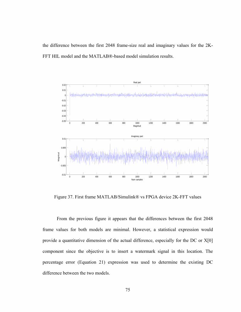
75
the difference between the first 2048 frame-size real and imaginary values for the 2K-
FFT HIL model and the MATLAB®-based model simulation results.
Figure 37. First frame MATLAB/Simulink® vs FPGA device 2K-FFT values
From the previous figure it appears that the differences between the first 2048
frame values for both models are minimal. However, a statistical expression would
provide a quantitative dimension of the actual difference, especially for the DC or X[0]
component since the objective is to insert a watermark signal in this location. The
percentage error (Equation 21) expression was used to determine the existing DC
difference between the two models.
0 200 400 600 800 1000 1200 1400 1600 1800 2000-0.05
-0.04
-0.03
-0.02
-0.01
0
0.01
0.02Real part
Magnitud
0 200 400 600 800 1000 1200 1400 1600 1800 2000-0.01
-0.005
0
0.005
0.01Imaginary part
Num samples
Magnitud

76
Where the theoretical or expected value T. value corresponds to the resulting
Simulink® -based program values and the experimental value E. Value is the 2K-FFT
HIL model DC value. The resulting %error value is 0.3498, which is very small. Thus,
we can conclude that the 2K-FFT HIL model satisfies the FFT performance. In order to
confirm this conclusion, another experimental test was performed. The Ks factor was
calculated using the resulting FFT values from the 2K-FFT HIL model and compared
with the Ks-factor Simulink® model shown in Figure 8. The resulting values were
1.2653 for the Simulink®-based model and 1.2654 for the 2K-FFT HIL model. Again,
we can affirm that the 2K-FFT HIL model has high performance.
Similarly to the host audio signal and watermarked signal comparison tests
mentioned in Section 3.5.1, the resulting watermarked signal A’ from the 2K-FFT HIL
model was compared with the original audio file A. Figures 38, 39, and 40 display the
resulting waveforms after comparison.

77
Figure 38. Track1 DC watermarking simulation waveforms -2K-FFT model
Figure 39. Track2 DC watermarking simulation waveforms -2K-FFT model
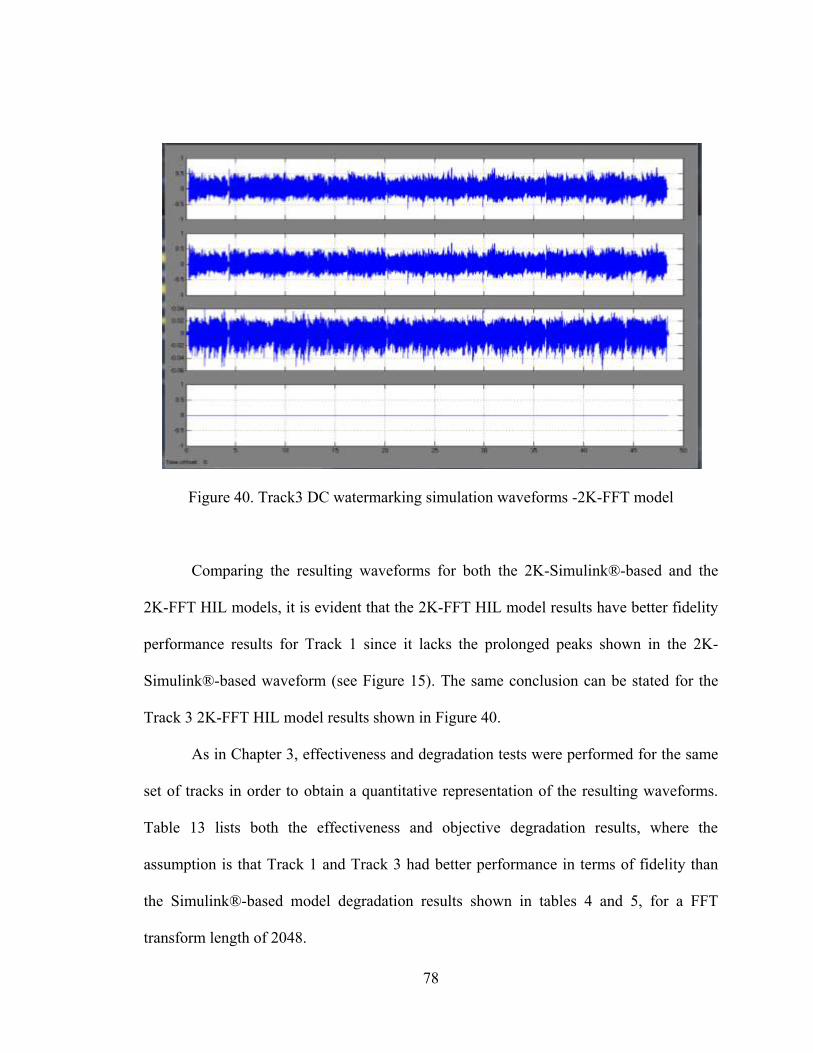
78
Figure 40. Track3 DC watermarking simulation waveforms -2K-FFT model
Comparing the resulting waveforms for both the 2K-Simulink®-based and the
2K-FFT HIL models, it is evident that the 2K-FFT HIL model results have better fidelity
performance results for Track 1 since it lacks the prolonged peaks shown in the 2K-
Simulink®-based waveform (see Figure 15). The same conclusion can be stated for the
Track 3 2K-FFT HIL model results shown in Figure 40.
As in Chapter 3, effectiveness and degradation tests were performed for the same
set of tracks in order to obtain a quantitative representation of the resulting waveforms.
Table 13 lists both the effectiveness and objective degradation results, where the
assumption is that Track 1 and Track 3 had better performance in terms of fidelity than
the Simulink®-based model degradation results shown in tables 4 and 5, for a FFT
transform length of 2048.

79
Table 13. Effectiveness and objective degradation metrics results -2K-FFT model
BER [%] MD AD MSE SNR [dB]
Track_1 0 0.0196 0.0038 2.147e-5 69.057 Track_2 0 0.0518 0.0055 6.237e-5 59.036 Track_3 0 0.0295 0.0040 2.435e-5 66.402
Moreover, an informal subjective degradation test or listening test performed for
each track indicates that Track 1 has slighter perceptible noise than the rest of the
watermarked tracks. To sum, the developed and implemented 2K-FFT HIL model is
suitable for the proposed DC audio watermarking scheme.
Similarly to the 2K-FFT HIL model performance test, the resulting FFT values of
the 1K-FFT HIL model were compared with the first 1024 Simulink®-based program
values. Figure 41 shows the real and imaginary part comparison values between both
models.
Figure 41. First frame MATLAB/Simulink® vs. FPGA device 1K-FFT values
0 100 200 300 400 500 600 700 800 900 1000-0.2
0
0.2Real
Magnitude
0 200 400 600 800 1000 1200-1
0
1Imaginary
Num Samples
Magnitude

80
Once again the difference appears to be minimal, which it is an expected result
since the only difference between the models is the FFT transforms length. Applying the
same percentage error expression, the resulting % error value is 0.2407, when the
expected value T. value is the Simulink® -based program DC result and the experimental
value E. Value corresponds to the 1K-FFT HIL model DC value. Additionally, the Ks
factor value obtained using the 1K-FFT HIL model is 1.0553 compared with the
Simulink®-based model Ks value of 1.0554. This difference is insignificant since the
resolution for the Ks factor difference is three decimals.
Figure 42 Track1 DC watermarking simulation waveforms -1K-FFT model

81
Figure 43. Track 2 DC watermarking simulation waveforms -1K-FFT model
Figure 44. Track3 DC watermarking simulation waveforms -1K-FFT model
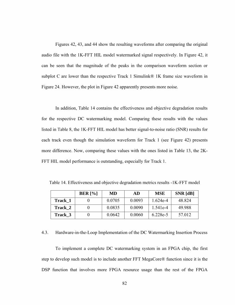
82
Figures 42, 43, and 44 show the resulting waveforms after comparing the original
audio file with the 1K-FFT HIL model watermarked signal respectively. In Figure 42, it
can be seen that the magnitude of the peaks in the comparison waveform section or
subplot C are lower than the respective Track 1 Simulink® 1K frame size waveform in
Figure 24. However, the plot in Figure 42 apparently presents more noise.
In addition, Table 14 contains the effectiveness and objective degradation results
for the respective DC watermarking model. Comparing these results with the values
listed in Table 8, the 1K-FFT HIL model has better signal-to-noise ratio (SNR) results for
each track even though the simulation waveform for Track 1 (see Figure 42) presents
more difference. Now, comparing these values with the ones listed in Table 13, the 2K-
FFT HIL model performance is outstanding, especially for Track 1.
Table 14. Effectiveness and objective degradation metrics results -1K-FFT model
BER [%] MD AD MSE SNR [dB]
Track_1 0 0.0705 0.0093 1.624e-4 48.824 Track_2 0 0.0835 0.0090 1.541e-4 49.988 Track_3 0 0.0642 0.0060 6.228e-5 57.012
4.3. Hardware-in-the-Loop Implementation of the DC Watermarking Insertion Process
To implement a complete DC watermarking system in an FPGA chip, the first
step to develop such model is to include another FFT MegaCore® function since it is the
DSP function that involves more FPGA resource usage than the rest of the FPGA
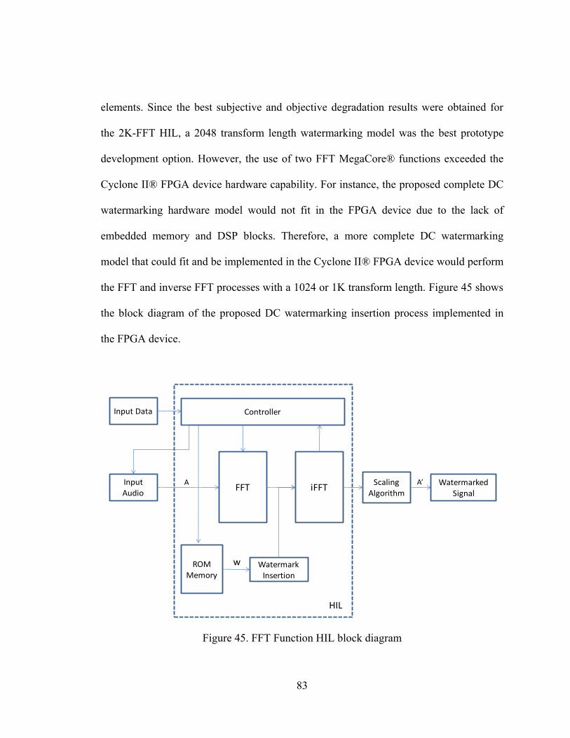
83
elements. Since the best subjective and objective degradation results were obtained for
the 2K-FFT HIL, a 2048 transform length watermarking model was the best prototype
development option. However, the use of two FFT MegaCore® functions exceeded the
Cyclone II® FPGA device hardware capability. For instance, the proposed complete DC
watermarking hardware model would not fit in the FPGA device due to the lack of
embedded memory and DSP blocks. Therefore, a more complete DC watermarking
model that could fit and be implemented in the Cyclone II® FPGA device would perform
the FFT and inverse FFT processes with a 1024 or 1K transform length. Figure 45 shows
the block diagram of the proposed DC watermarking insertion process implemented in
the FPGA device.
Figure 45. FFT Function HIL block diagram
ScalingAlgorithm
InputAudio
FFT
Input Data Controller
HIL
A’A Watermarked Signal
iFFT
ROM Memory
WatermarkInsertion
w

84
In the figure above, it is observed that the controller has to ensure the correct data
flow in four DSP blocks, such as the ROM memory and the two FFT blocks. This
required an algorithmic alteration on the previous controller code as well as on the
Scaling Algorithm block. Since the output on this particular block corresponds to the
resulting watermarked signal A‟, the scaling expression is therefore defined as [25]:
Where iFFTouput is the real output value and exp1 and exp2 correspond to the
number of shifts for the FFT and iFFT blocks, respectively. Another significant alteration
in the DC watermarking algorithm is the absence of the PSD Analysis process since it
would require more memory capacity to perform the power spectral density of each
frame and multiply it by the scaling Ks factor. The alternative algorithm suggests
multiplying solely the DC component by the binary watermark signal. Thus, the
embedded watermark signal W is expressed as the following expression:
Where W is the embedded watermark signal, is the nth DC component of
the host audio signal and w the binary watermark signal. In this alternative DC
watermarking insertion process scheme, the binary watermark signal is stored in an on-
chip ROM memory of the Cyclone II® FPGA chip.

85
4.3.1. MATLAB/Simulink® and DSP Builder Model Description
Figure 46 shows the alternative HIL DC watermarking insertion process model in
Simulink®. The HIL block shown in this figure contains the necessary DSP blocks to
embed the watermark signal according to the block diagram in Figure 45.
Figure 46. Alternative HIL DC watermarking insertion process model
A MATLAB® file reads the host audio signal to get some important input data to
set the some constants such as the Ks factor and number of frames. After the DC
watermark insertion is done, the resulting watermarked signal A’ can be extracted by the
watermark extraction process described in Section 3.4 in order to test the effectiveness of
the alternative DC watermarking model.

86
Figure 47 shows part of the alternative DC watermarking RTL circuit. In contrast
with the RTL diagram of the 1K-FFT HIL model in Figure 32, this DSP system contains
a larger number of embedded elements inside each instantiated VHDL component.
Figure 47. Part of the alternative DC watermarking RTL view
4.3.2. On-chip Single-Port ROM Memory
The Cyclone II® FPGA device has embedded M4K memory blocks that are pre-
initialized using a MATLAB® file [24] and [26]. In the proposed DC watermarking
insertion model a 1024x1 ROM memory is implemented with an input address port and
an output port. The DSP Builder library provides both ROM and RAM memories blocks
that map stored data to the internal FPGA device.
The watermark insertion process for the alternative DC audio watermarking
scheme is represented in Figure 41. This figure contains the ROM memory and

87
configuration circuit of three multiplexers. The complete circuit also satisfied the
expression in Equation (23), where the DC component is multiplied by the binary
watermark signal w. The function of the ROM memory is to store the watermark signal in
the embedded memory of the FPGA device.
Figure 48. Alternative DC watermark insertion using DSP blocks
Following the DSP blocks in Figure 48, an additional controller is implemented to
manage the insertion of the watermark signal. Figure 49 shows a simple example of how
the extra controller performs the watermark insertion. Based on Equation (23) and the
FFT MegaCore® function control signals, the SOP signal is asserted to indicate the start
of the frame. In other words, the SOP signal indicates when the FFT block outputs the
DC or X[0] component. Taking that event as a flag or indicator, the controller reads the
SOP signal and changes the ROM memory address when a start of frame occurs indicated
by the SOP signal. Moreover, the controller has an enable control signal that ensures the
complete watermark insertion. After the watermark has been inserted the enable signal
goes to a neutral value.
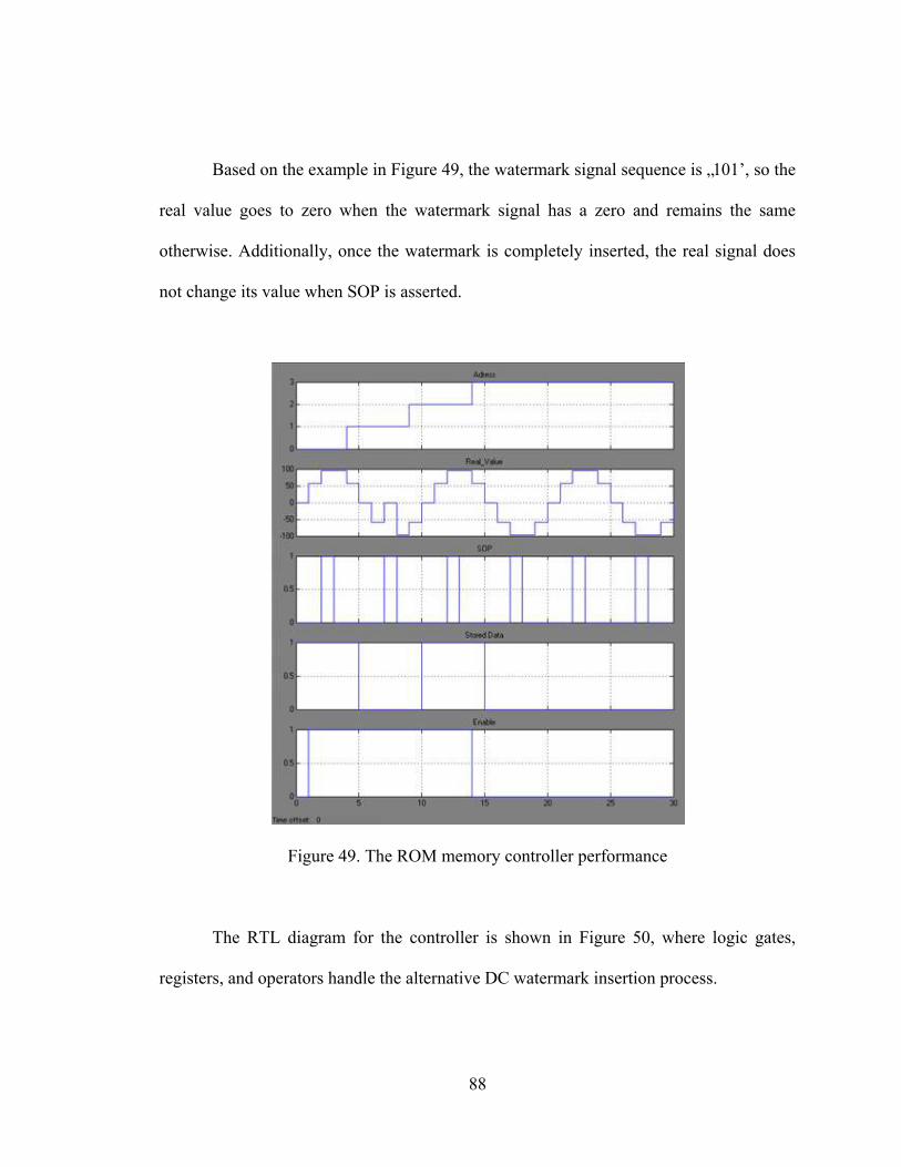
88
Based on the example in Figure 49, the watermark signal sequence is „101‟, so the
real value goes to zero when the watermark signal has a zero and remains the same
otherwise. Additionally, once the watermark is completely inserted, the real signal does
not change its value when SOP is asserted.
Figure 49. The ROM memory controller performance
The RTL diagram for the controller is shown in Figure 50, where logic gates,
registers, and operators handle the alternative DC watermark insertion process.
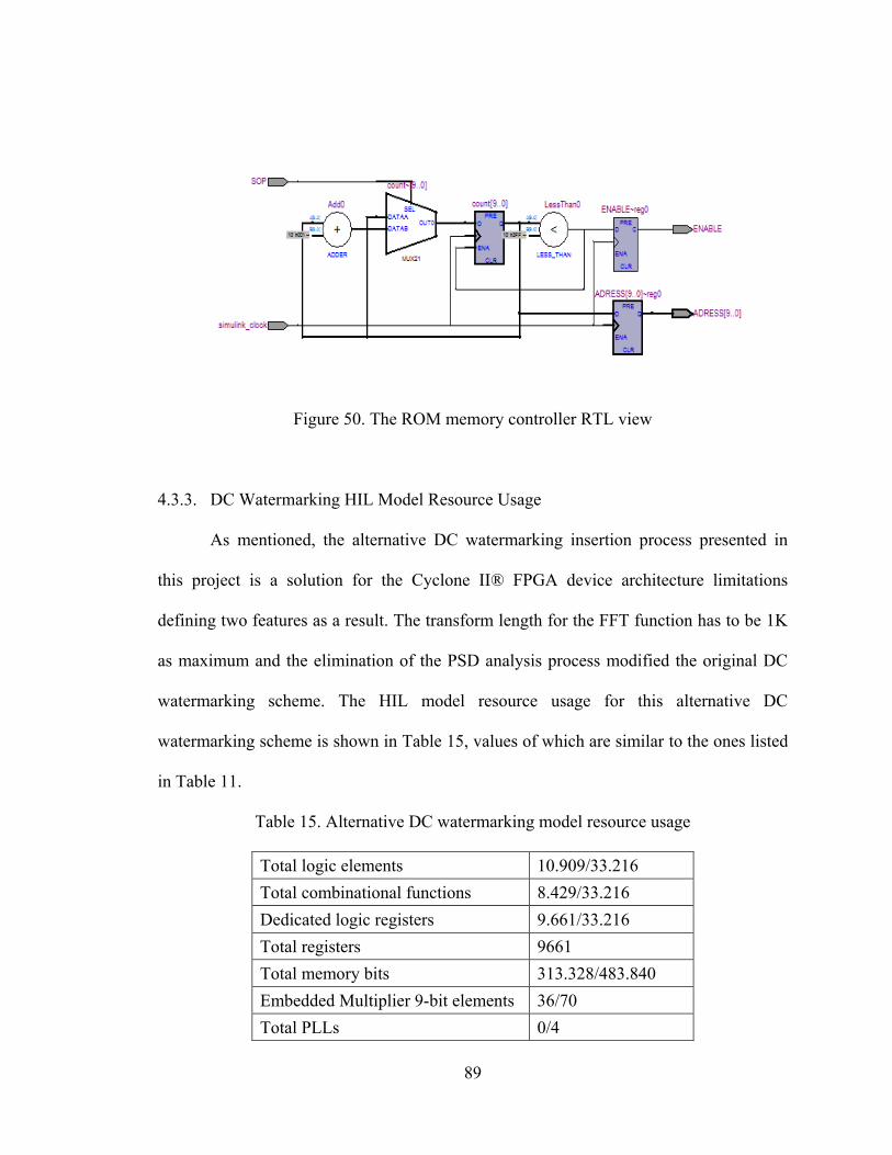
89
Figure 50. The ROM memory controller RTL view
4.3.3. DC Watermarking HIL Model Resource Usage
As mentioned, the alternative DC watermarking insertion process presented in
this project is a solution for the Cyclone II® FPGA device architecture limitations
defining two features as a result. The transform length for the FFT function has to be 1K
as maximum and the elimination of the PSD analysis process modified the original DC
watermarking scheme. The HIL model resource usage for this alternative DC
watermarking scheme is shown in Table 15, values of which are similar to the ones listed
in Table 11.
Table 15. Alternative DC watermarking model resource usage
Total logic elements 10.909/33.216 Total combinational functions 8.429/33.216 Dedicated logic registers 9.661/33.216 Total registers 9661 Total memory bits 313.328/483.840 Embedded Multiplier 9-bit elements 36/70 Total PLLs 0/4

90
Additionally, Figure 51 has a similar relation in terms of resource usage
percentage with the plot in Figure 35. Moreover, the alternative DC watermarking
insertion model had a simulation rate of 1.9 minutes per second of sound processed. To
sum, the alternative DC watermarking scheme is a cost-effective DSP system since it is
performing a complete DC watermark insertion process in the same FPGA device, using
similar resource usage for a 2K length FFT process, as described in Figure 35.
Figure 51. Alternative DC watermarking resource usage percentage plot
4.3.4. HIL Model Performance and MATLAB/Simulink® System Comparison
To test the performance of the alternative DC watermarking insertion model
implemented in the Cyclone II® FPGA device, this DSP system was evaluated under the
same performance tests in order to obtain representative results in a fair DC
watermarking scheme comparison. To obtain a visual comparison between the original
audio and the watermarked signal, the same Simulink® model plotted the original,
watermarked signals with their respective resulting comparison test results. Additionally,
25 % 29 % 65 % 51 %
0%
10%
20%
30%
40%
50%
60%
70%
Total combinational
functions
Dedicated logic registers
Total memory bits
Embedded Multiplier 9-bit
elements

91
the error variable (see Equation 11) provides the incorrect watermark extracted bits
during the DC watermark extraction process. The resulting Track 1 waveforms are
displayed in Figure 52, where the audio files comparison waveform (subplot C) has a
similar result as the plot in Figure 24. In both experimental cases, the length of the FFT
function is 1024. Moreover, the resulting comparison waveform of the alternative DC
watermarking insertion model has fewer peaks than the waveform in Figure 42.
In other words, comparing the three 1K transform length DC watermarking
models, the alternative DC watermarking insertion process has visually better fidelity
performance than the implemented FFT HIL model (see Figure 42) and similar
performance to the Simulink®-based model in Figure 24.
Figure 52. Track1 alternative DC watermarking simulation waveforms

92
Running the same performance tests, the effectiveness and degradation tests for
alternative DC watermarking schemes were evaluated, where the results are listed in
Table 16. In terms of effectiveness, the watermarked signal was unsuccessfully extracted
since Figure 45 shows incorrect extracted bits during the watermark extraction process.
The resulting BER number is 10.8% which can be acceptable for a 1K width watermark
signal. Against visual fidelity performance prediction, the objective degradation results
show that the implemented FFT HIL model has better fidelity performance than the
alternative DC watermarking. This also can be prove in an informal listening test, where
the alternative scheme contains a little more noise than the 1K-FFT HIL model.
Table 16. Effectiveness and degradation results - Alternative DC watermarking model
BER [%] MD AD MSE SNR [dB]
Track_1 10.8 0.0695 0.0187 5.172e-4 39.857

93
CHAPTER 5
CONCLUSIONS AND FUTURE WORK
This thesis presented a brief description of audio watermarking applications and
algorithms to introduce the direct current (DC) audio watermarking scheme. Like most
watermarking schemes, the proposed audio watermarking algorithm requires two crucial
processes to achieve the watermarking, namely insertion and extraction, where the
watermark signal is embedded in the host audio signal. Audio watermarking systems like
the DC watermarking have the purpose of embedding a watermark signal without
producing any perceptible alteration in the original audio file, so that the watermark
signal is imperceptible to the human auditory system. Another watermarking
characteristic is that the embedded watermark has to remain in the host signal after
several signal processing attacks, such as cropping and audio compression. This
watermark characteristic is called robustness and is one of most analyzed properties due
to the wide range of capabilities that can be designed in a real-world application.
In order to design and develop an imperceptible and robust audio watermarking
system, a DC audio watermarking model is proposed using MATLAB® [9] and
Simulink® [9] programming software. The prototyping design flow is described in
Chapters 2 and 3. In Chapter 3 the MATLAB/Simulink® DC watermarking model is
described, where a set of three audio files were used during the simulations.

94
In general, the proposed software-based watermarking model can be divided in
two main parts, one for the DC watermarking insertion process and the other for the
extraction process.
Based on the DC audio watermarking algorithm described in Chapter 2, two
watermarking models were designed using MATLAB/Simulink®. The main distinction
between these models is the Fourier transform length, the values of which are 1024 and
2048. Several tests were conducted to evaluate the effectiveness and fidelity performance
of the two DC watermarking models. To visually evaluate both watermarking
characteristics, a Simulink® model plots the original audio signal, the watermarked
signal, the difference between them, and the event when an incorrect bit is extracted.
Additionally, some quantitative measures were also included in the tests in order to
quantify the DC watermarking performance. Among them, the most representative
measures are the signal-to-noise ratio (SNR) and the bit error rate (BER) for the
effectiveness and fidelity performance respectively. Table 5 listed the resulting values for
the 2048 transform length DC watermarking model, whereas Table 8 listed them for the
1024 model. Based on these results, Track 3 has better fidelity performance in both
models since the resulting SNR is around 42-43dB. However, a visual inspection on the
resulting simulation waveforms indicates that Track 1 has less added noise for the 2048
transform length DC watermarking model. Additionally, an informal listening test
confirms that assumption, indicating that the measure of the SNR does not always reflect
95
the actual perceptual noise. This case is also presented between Tracks 1 and 3 in table 8.
Whereas Track 3 has a better SNR result, Track 1 has lower perceptible noise.
In order to achieve better effectiveness and fidelity performances results in the
proposed DC audio watermarking model, a Cyclone® II [8] device form Altera® [8] was
used to create a software-hardware-in-the-loop audio watermarking model. To reach this
goal, the use of the Altera® DSP Builder [8] tool makes the field-programmer gate array
(FPGA) hardware implementation compatible with MATLAB® and Simulink®. The
final DC audio watermarking model implemented in a FPGA device is shown in Figure
29, where the fast Fourier transform (FFT) function is computed in the FPGA device.
Tables 13 and 14 list the effectiveness and objective degradation performance results for
the 2K-FFT length and the 1K-FFT length models. Comparing these results, the 2048
transform length DC watermarking model implemented in the FPGA shows better
fidelity results than the 1K-FFT length model. On the other hand, by comparing the
MATLAB/Simulink®-based DC watermarking performance results with the software-
hardware-in-the-loop audio watermarking model results, it is evident that the FPGA
hardware implementation approach produced better fidelity results. In particular, the SNR
value in the 2K-FFT length DC audio watermarking model is in the range of 59-69 dB.
This outstanding result is even better to other experimental results for more complex
audio watermarking schemes presented in several papers [1], [19], [22], and [27].
Moreover, the conducted informal listening tests also showed better performance results
for the 2K-FFT length DC audio watermarking model implemented in the Cyclone® II
FPGA device. Figure 53 shows the resulting waveforms for the original and watermarked
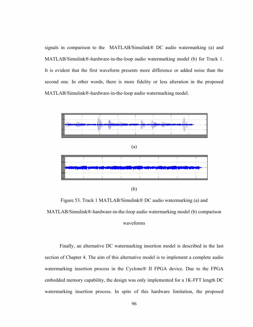
96
signals in comparison to the MATLAB/Simulink® DC audio watermarking (a) and
MATLAB/Simulink®-hardware-in-the-loop audio watermarking model (b) for Track 1.
It is evident that the first waveform presents more difference or added noise than the
second one. In other words, there is more fidelity or less alteration in the proposed
MATLAB/Simulink®-hardware-in-the-loop audio watermarking model.
(a)
(b)
Figure 53. Track 1 MATLAB/Simulink® DC audio watermarking (a) and
MATLAB/Simulink®-hardware-in-the-loop audio watermarking model (b) comparison
waveforms
Finally, an alternative DC watermarking insertion model is described in the last
section of Chapter 4. The aim of this alternative model is to implement a complete audio
watermarking insertion process in the Cyclone® II FPGA device. Due to the FPGA
embedded memory capability, the design was only implemented for a 1K-FFT length DC
watermarking insertion process. In spite of this hardware limitation, the proposed

97
alternative DC watermarking insertion algorithm, expressed in Equation 23, produced
satisfactory performance results as shown in Figure 52 and Table 16.
To conclude, the 2K-FFT MATLAB/Simulink®-hardware-in-the-loop audio
watermarking model presents better performance results in terms of fidelity and
effectiveness. However, the alternative DC watermarking insertion model shows
acceptable performance results in almost the same FPGA resource usage as the 2K-FFT.
Based on the experimental results presented in Chapter 3 and Chapter 4,
additional work is necessary to be done in order to improve the presented DC audio
watermarking models implemented in a FPGA device. First, a new set of audio tracks has
to be tested. This set has to include audio files from different music genres such as pop,
rock, and classical genres [19]. Additionally, the DC audio watermarking model must be
suitable for stereophonic music. This specification might involve more memory
resources; however, redundancy in the watermark insertion process can be implemented
since small watermark signals are embedded through the audio file [27] and [28].
The use of external memory instead of embedded memory in the FPGA will lead
to a high performance digital audio watermarking. For instance, the Cyclone® II FPGA
device provides an 8MB SDRAM (synchronous dynamic random access memory) [26]
that can be implemented to improve the proposed DC audio watermarking scheme shown
in Chapter 2. In addition, this device also includes a secure digital (SD) memory card
slot, where a complete DC watermarking scheme can be implemented in a FPGA device.
Moreover, real-time DC audio watermarking system can be achieved, where the
watermark signal is embedded while capturing the input audio signal.

98
Once the mentioned future work to obtain a complete DC watermarking model
implemented in a FPGA chip is achieved, experimental performance tests can be
conducted such as capacity, robustness and fidelity tests. For the last one, a formal
subjective degradation test can be performed based on the International
Telecommunication Union (ITU), based on [19] and [22], where trained listeners
evaluate the perceptible audio degradation made during the watermark insertion process
using a graded impairment scale.
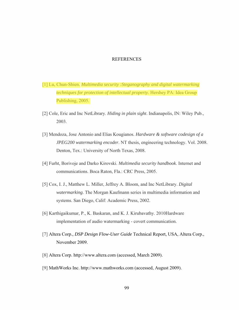
99
REFERENCES
[1] Lu, Chun-Shien. Multimedia security :Steganography and digital watermarking
techniques for protection of intellectual property. Hershey PA: Idea Group
Publishing, 2005.
[2] Cole, Eric and Inc NetLibrary. Hiding in plain sight. Indianapolis, IN: Wiley Pub.,
2003.
[3] Mendoza, Jose Antonio and Elias Kougianos. Hardware & software codesign of a
JPEG200 watermarking encoder. NT thesis, engineering technology. Vol. 2008.
Denton, Tex.: University of North Texas, 2008.
[4] Furht, Borivoje and Darko Kirovski. Multimedia security handbook. Internet and
communications. Boca Raton, Fla.: CRC Press, 2005.
[5] Cox, I. J., Matthew L. Miller, Jeffrey A. Bloom, and Inc NetLibrary. Digital
watermarking. The Morgan Kaufmann series in multimedia information and
systems. San Diego, Calif: Academic Press, 2002.
[6] Karthigaikumar, P., K. Baskaran, and K. J. Kirubavathy. 2010Hardware
implementation of audio watermarking - covert communication.
[7] Altera Corp., DSP Design Flow-User Guide Technical Report, USA, Altera Corp.,
November 2009.
[8] Altera Corp. http://www.altera.com (accessed, March 2009).
[9] MathWorks Inc. http://www.mathworks.com (accessed, August 2009).

100
[10] Altera Corp., DSP Builder Reference User Guide Technical Report, USA, Altera
Corp., November 2009.
[11] Perez-Gonzalez, F. and J. R. Hernandez. 1999 A tutorial on digital watermarking.
[12] Liu, Z. and A. Inoue. Audio watermarking techniques using sinusoidal patterns
based on pseudorandom sequences. Circuits and Systems for Video Technology,
IEEE Transactions on 13, no. 82003). : 801-812.
[13] Jajodia, Neil F. Johnson, Zoran Duric, and Sushil. Information hiding:
Steganography and watermarking - attacks and countermeasures Springer, 2000.
[14] Megías, David, Jordi Herrera-Joancomartí, and Julià Minguillón. 2004 An audio
watermarking scheme robust against stereo attacks. Magdeburg, Germany, ACM,.
[15] Lang, Andreas, Jana Dittmann, Ryan Spring, and Claus Vielhauer. 2005 Audio
watermark attacks: From single to profile attacks. New York, NY, USA, ACM, .
[16] Cox, I. J., J. Kilian, F. T. Leighton, and T. Shamoon. Secure spread spectrum
watermarking for multimedia. Image Processing, IEEE Transactions on 6, no.
121997). : 1673-1687.
[17] Megías, David, Jordi Herrera-Joancomartí, and Julià Minguillón. A robust audio
watermarking scheme based on MPEG 1 layer 3 compression. In
Communications and multimedia security, ed. Antonio Lioy and Daniele
Mazzocchi. Vol. 2828, 226-238Springer Berlin / Heidelberg, 2003.
[18] Changsheng Xu, Jiankang Wu, and Qibin Sun. 1999 Digital audio watermarking and
its application in multimedia database.
[19] Malik, H., R. Ansari, and A. Khokhar. Robust audio watermarking using frequency-
selective spread spectrum. Information Security, IET 2, no. 42008). : 129-150.

101
[20] Audio Box, http://www.ece.uvic.ca/~aupward/w/watermarking (accessed, June
2009).
[21] MathWorks Inc., Signal Processing blockset 7 User’s Guide, Technical Report,
USA, MathWorks, September 2010.
[22] Huan Li, Zheng Qin, and Liping Shao. 2009 Audio watermarking pre-process
algorithm.
[23] Yong-Jae Jeong, Won-Hee Kim, Kwang-Seok Moon, and Jong-Nam Kim. 2008
Implementation of watermark detection system for hardware based video
watermark embedder.
[24] Altera Corp., DSP Builder Reference Manual ,Technical Report USA, Altera Corp.,
November 2009.
[25] Altera Corp., FFT MegaCore Function- User Guide ,Technical Report USA, Altera
Corp., November 2009.
[26] Altera Corp., Internal Memory (RAM and ROM) - User Guide ,Technical Report
,USA, Altera Corp., November 2009.
[27] Li, W., X. Y. Xue, and X. Q. Li. 2003 Localized robust audio watermarking in
regions of interest.
[28] Lach, J., W. H. Mangione-Smith, and M. Potkonjak. 1999 Robust FPGA intellectual
property protection through multiple small watermarks.