auditory-based time-frequency representations …...auditory-based time-frequency representations...
TRANSCRIPT

Auditory-Based Time-FrequencyRepresentations and Feature
Extraction Techniques for SonarProcessing
CS-05-12
October 2005
Robert Mill and Guy Brown
Speech and Hearing Research GroupDepartment of Computer Science
University of Sheffield


Abstract
Passive sonar classification involves identifying underwater sources by thesound they make. A human sonar operator performs the task of classifica-tion both by listening to the sound on headphones and looking for features ina series of ‘rolling’ spectrograms. The construction of long sonar arrays con-sisting of many receivers allows the coverage of several square kilometres inmany narrow, directional beams. Narrowband analysis of the signal withinone beam demands considerable concentration on the part of the sonar oper-ator and only a handful of the hundred beams can be monitored effectivelyat a single time. As a consequence, there is an increased requirement for theautomatic classification of sounds arriving at the array.
Extracting tonal features from the signal—a key stage of the classificationprocess—must be achieved against a broadband noise background contributedby the ocean and vessel engines. This report discusses potential solutions to theproblem of tonal detection in noise, with particular reference to models of thehuman ear, which have been shown to provide a robust encoding of frequencycomponents (e.g. speech formants) in the presence of additive noise.
The classification of sonar signals is complicated further by the presence ofmultiple sources within individual beams. As these signals exhibit consider-able overlap in the frequency and time domain, some mechanism is requiredto assign features in the time-frequency plane to distinct sources. Recent re-search into computational auditory scene analysis has led to the development ofmodels that simulate human hearing and emphasise the role of the ears andbrain in the separation of sounds into streams. The report reviews these modelsand investigates their possible application to the problem of concurrent soundseparation for sonar processors.
3


Contents
1 Introduction 71.1 Composition of Sonar Signals . . . . . . . . . . . . . . . . . . . . 8
1.1.1 Vessel Acoustic Signatures . . . . . . . . . . . . . . . . . . 81.1.2 Sonar Analysis . . . . . . . . . . . . . . . . . . . . . . . . 9
1.2 Anatomy and Function of the Human Ear . . . . . . . . . . . . . 91.2.1 The Outer Ear . . . . . . . . . . . . . . . . . . . . . . . . . 101.2.2 The Middle Ear . . . . . . . . . . . . . . . . . . . . . . . . 101.2.3 The Cochlea and Basilar Membrane . . . . . . . . . . . . 101.2.4 Hair Cell Transduction . . . . . . . . . . . . . . . . . . . . 101.2.5 The Auditory Nerve . . . . . . . . . . . . . . . . . . . . . 11
1.3 Perceiving Sound . . . . . . . . . . . . . . . . . . . . . . . . . . . 121.3.1 Masking and the Power Spectrum Model . . . . . . . . . 121.3.2 Pitch . . . . . . . . . . . . . . . . . . . . . . . . . . . . . . 121.3.3 Modulation . . . . . . . . . . . . . . . . . . . . . . . . . . 13
1.4 Auditory Scene Analysis . . . . . . . . . . . . . . . . . . . . . . . 141.5 Chapter Summary . . . . . . . . . . . . . . . . . . . . . . . . . . . 16
2 Auditory Modelling 172.1 Modelling the Auditory Periphery . . . . . . . . . . . . . . . . . 17
2.1.1 The Outer and Middle Ear Filter . . . . . . . . . . . . . . 172.1.2 Basilar Membrane Motion . . . . . . . . . . . . . . . . . . 172.1.3 Hair Cell Transduction . . . . . . . . . . . . . . . . . . . . 19
2.2 Computational Auditory Scene Analysis . . . . . . . . . . . . . . 202.3 Auditory Modelling in Sonar . . . . . . . . . . . . . . . . . . . . 232.4 Summary . . . . . . . . . . . . . . . . . . . . . . . . . . . . . . . . 26
3 Time-Frequency Representations and the EIH 293.1 Signal Processing Solutions . . . . . . . . . . . . . . . . . . . . . 29
3.1.1 Short-time Fourier Transform . . . . . . . . . . . . . . . . 293.1.2 Wigner Distribution . . . . . . . . . . . . . . . . . . . . . 303.1.3 Wavelet Transform . . . . . . . . . . . . . . . . . . . . . . 30
3.2 Ensemble Interval Histogram . . . . . . . . . . . . . . . . . . . . 313.2.1 Model . . . . . . . . . . . . . . . . . . . . . . . . . . . . . 313.2.2 Properties . . . . . . . . . . . . . . . . . . . . . . . . . . . 323.2.3 Analysis of Vowels . . . . . . . . . . . . . . . . . . . . . . 343.2.4 Analysis of Sonar . . . . . . . . . . . . . . . . . . . . . . . 363.2.5 Using Entropy and Variance . . . . . . . . . . . . . . . . . 38
3.3 Summary and Discussion . . . . . . . . . . . . . . . . . . . . . . 41
5

CONTENTS
4 Feature Extraction 434.1 Lateral Inhibition . . . . . . . . . . . . . . . . . . . . . . . . . . . 43
4.1.1 Shamma’s Lateral Inhibition Model . . . . . . . . . . . . 444.1.2 Modelling Lateral Inhibition in MATLAB . . . . . . . . . 464.1.3 Discussion . . . . . . . . . . . . . . . . . . . . . . . . . . . 49
4.2 Peak Detection and Tracking . . . . . . . . . . . . . . . . . . . . . 504.2.1 Time-frequency Filtering . . . . . . . . . . . . . . . . . . . 504.2.2 Peak Detection . . . . . . . . . . . . . . . . . . . . . . . . 504.2.3 Peak Tracking . . . . . . . . . . . . . . . . . . . . . . . . . 54
4.3 Modulation Spectrum . . . . . . . . . . . . . . . . . . . . . . . . 554.3.1 Computing the Modulation Spectrum . . . . . . . . . . . 564.3.2 Suitability for Sonar . . . . . . . . . . . . . . . . . . . . . 57
4.4 Phase Modulation . . . . . . . . . . . . . . . . . . . . . . . . . . . 574.4.1 Phase-tracking using the STFT . . . . . . . . . . . . . . . 584.4.2 Measuring Fluctuations . . . . . . . . . . . . . . . . . . . 594.4.3 The Effect of Noise . . . . . . . . . . . . . . . . . . . . . . 614.4.4 Non-linear Filtering . . . . . . . . . . . . . . . . . . . . . 62
5 Conclusions and Future Work 655.1 Future Work . . . . . . . . . . . . . . . . . . . . . . . . . . . . . . 65
6
Chapter 1
Introduction
The undersea acoustic environment comprises a rich mixture of sounds, bothman-made and natural in origin. Examples of these include vessel engines,sonar pings, shoreside industry, snapping shrimp, whale vocalisations andrain. The energy in electromagnetic waves (including visible light) is absorbedrapidly by sea water, so sound waves, which can propagate over many kilo-metres, remain the principal carrier of information about the environment. Inits simplest incarnation, sonar classification is the procedure of listening to andidentifying these underwater sounds, and is an essential military tool for de-termining whether a seaborne target is hostile or friendly, natural or unnatural.
Modern sonar analysis is performed by a human expert who listens to thesound in a single directional beam and makes a judgement as to what can beheard. In conjunction with an aural analysis, spectrograms of the sound withineach beam are presented on visual displays. The manufacture of longer sonararrays has led to a commensurate increase in the number of beams to which anoperator must attend. In order to reduce this load, there have been numerousattempts to perform the classification of sonar signals using a machine. How-ever, such attempts have been frustrated by the presence of interfering sourceswithin a beam—a second vessel, or biological sounds, for example.
The difficulty in isolating individual sounds from a mixture has been en-countered in other technology areas, a notable example being automatic speechrecognition (ASR) systems, whose performance degrades in the presence ofmultiple talkers or interference from the environment. Human beings, on theother hand, are able to decipher and attend to individual sources within a mix-ture of sounds as a matter of course, e.g. the voice of speaker in a crowd. Inrecent years, computational models of hearing have emerged, which aim toexplain and emulate this listening process. Improved ASR, intelligent hearingaids and automatic music transcription have all been cited as techologies thatcould benefit from such an auditory approach.
This report presents automatic sonar classification as a listening activity andconsiders how the recent advances in computational hearing may assist a hu-man sonar operator in managing the increasing quantity of data from the array.Following a literature survey, methods of signal extraction from noisy data us-ing models of the ear are examined. Later sections discuss the possibility ofsource separation and tonal grouping by exploiting correlated changes in sig-nal properties, such as amplitude and phase.
7

Chapter 1. Introduction
1.1 Composition of Sonar Signals
Sonar (sound navigation and ranging) systems detect and locate underwaterobjects by measurement of reflected or radiated sound waves and may be cat-egorised as either active or passive systems. [30] Active sonar systems transmita brief pulse or ‘ping’ and await the return of an echo, for example, against thehull of a vessel; the delay and direction of the echo reveal the distance and bear-ing of the target, respectively. Active sonar is considered unsuitable for manymilitary applications as the transmission of a ping can easily reveal the locationof the sonar platform to hostile targets. In addition, the two-way propagationloss incurred by echo-ranging restricts the radius over which active systemscan operate effectively. Passive sonar systems use an array of hydrophones toreceive sound radiated by the target itself, for example, the noise from the en-gine and propeller of a vessel. Analysis of the received signal allows a target tobe classified according to features of its time-varying spectrum, an advantagenot afforded by an active system. Work conducted in this project is based onthe passive sonar model; active sonar is not considered further.
1.1.1 Vessel Acoustic Signatures
Burdic [5] defines the acoustic signature of a vessel as follows:
The target acoustic signature is characterized by the radiated acous-tic spectrum level at a reference distance of 1m from the effectiveacoustic center of the target.
For practical purposes, the content of the idealised spectrum at one metre is notavailable and must be inferred from measurements made at the hydrophonearray using a spherical spreading law. The acoustic path between the sourceand receiver can appreciably modify the spectrum even at a short distance (lessthan two-hundred metres).
Vessel acoustic signatures consist of a series of discrete lines or tonals, whichmay or may not be harmonically related, immersed in a continuous, broad-band noise spectrum. The tonal components appear in the range 0–2kHz andarise chiefly as a consequence of the periodic motion of the machinery andpropellers along with any hull resonances that these actuate. The relative in-tensities and frequencies of the tonals, which provide salient features for targetclassification, are catalogued by the military and are often highly classified.
The broadband component can be ascribed to hydrodynamic noise andcavitation (tiny bubbles which form at the propeller) and obscures the dis-crete lines with increasing frequency such that a crossover point can be iden-tified above which the tonal components can no longer be discerned. [30] Thecrossover point for a merchant ship lies between 100Hz and 500Hz. As theship’s speed increases, the contribution from the broadband sources becomedominant and the crossover point is lower.
In addition to the stationary spectrum, transient events contribute to thereceived signal. These may arise from the target (e.g. a wrench being dropped,chains clanking), or other interfering sources, such as objects colliding with ahydrophone or biological sounds (e.g. cetacea, snapping shrimp). Figure 1.1illustrates some of these features. Throughout this document, spectrograms for
8

1.2. Anatomy and Function of the Human Ear
Frequency (Hz)
Tim
e (s
)
0 200 400 600 800 1000
0
20
40TONALS
TRANSIENT
Figure 1.1: A sonar spectrogram showing (i) a series of tonal components (ver-tical lines), (ii) a transient click (horizontal line), and (iii) low-frequency AMmodulated noise above 500Hz.
sonar will be presented in a waterfall format, with frequency on the abscissaand time displayed down the ordinate. Spectrograms for speech will follow theconvention of having time on the abscissa and frequency on the ordinate.
1.1.2 Sonar Analysis
Pressure waves arriving at the sonar platform are first transduced into elec-trical signals by an array of hydrophones. Introducing artificial phase delaybetween these signals at different frequencies permits a certain degree of direc-tivity dependent upon the hydrophone spacing and array length. This over-all process is referred to as beamforming. The sound received at the array ispresented to a human sonar operator via a combination of audition and nar-rowband and broadband visual displays. The broadband display shows theenergy at a bearing (on the abscissa) and time (on the ordinate) by mappingeach cell to a colour or greyscale value and so reveals the motion of contacts inrelation to the platform. There are two types of narrowband display: LOFAR(low-frequency analysis and recording) and DEMON (demodulation of noise).The LOFARgram comprises a column of waterfall spectrograms, each of whichcorresponds to the signal received in a beam, and allows the operator to clas-sify vessels and determine changes in Doppler—the shift in pitch which resultsfrom a vessel moving in its own sound field. The DEMON display shows themodulation components present in the envelope of the broadband signal andreveals the number of propellers and blades and their rate of rotation. As wellas using visual displays, the sonar operator can listen to a selected beam andmake decisions based on recognised sounds; in practice, the visual and audi-tory evidence complement each other.
1.2 Anatomy and Function of the Human Ear
The ear is the sense organ for hearing and is responsible for converting soundin the environment into nerve activity which can be interpreted by the brain.This section provides a brief overview of the structures of ear, which will bereferred to in later sections; a full treatment of the physiology of the ear can befound in Pickles. [17]
9

Chapter 1. Introduction
1.2.1 The Outer Ear
The outer ear consists of the pinna (the visible structure on the side of the head)and meatus or auditory canal, a tunnel-like cavity leading to the typanic mem-brane or eardrum. The outer ear serves a threefold purpose: first, to redirectof sound waves from the environment into the head; second, to increase thesound pressure at the tympanic membrane; and third, to assist in the localisa-tion of sound sources about the head. The pressure gain at the eardrum canbe attributed to the resonances of the meatus, together with the bowl-shaped,inner cavity of the pinna (the concha), which have the overall effect of broadlyboosting frequencies around 2.5kHz by 15-20dB. A second, lesser peak appearsat 5.5kHz, for which the concha is solely responsible.
1.2.2 The Middle Ear
The middle ear consists of the tympanic membrane and three small bonescalled the incus (’hammer’), malleus (’anvil’) and stapes (’stirrup’), collectivelyreferred to as the ossicles. The prongs of the stapes are connected to the ovalwindow of the cochlea. The middle ear is required to match the difference inacoustic impedance between the air in the meatus and the fluid in the cochlea,as allowing sound waves to directly propagate across the boundary wouldresult in most of the energy being reflected. This impedance matching canbe appreciated by considering that the area of the tympanic membrane is fargreater than that of the oval window, so conducting forces from the larger tothe smaller area results in a pressure increase. The mechanical levering actionof the ossicles themselves has also been shown to contribute to the impedancematch to a small extent. The middle ear, like the outer, has a transfer functionassociated with it, which has a smooth band-pass characteristic and peaks atabout 1kHz.
1.2.3 The Cochlea and Basilar Membrane
The cochlea is a coiled structure that is divided along its length into three fluid-filled compartments: the scala vestibuli, scala media and scala tympani. Theboundaries between the respective scalae are Reissner’s membrane and thebasilar membrane (BM). The membraneous oval window, which projects ontothe scala vestibuli, is displaced by the motion of the stapes and, as a result,generates a wave, which propagates through the fluid in the scala vestibuliand scala tympani and finally terminates at the round window. The motion ofthe fluid in the two chambers induces a wave in the basilar membrane. Theresponse of the BM to a sinusoidal stimulus is a wave at the same frequency;however, the displacement is maximal at a single place (the characteristic fre-quency) owing to the varying mechanical properties of the BM along its length(it is narrower and stiffer at the basal end). In this way, the BM performs theinitial of spectral decomposition of a stimulus.
1.2.4 Hair Cell Transduction
The physical motion of the basilar membrane is encoded into neural activityin a process known as hair-cell transduction. The basilar membrane runs in
10

1.2. Anatomy and Function of the Human Ear
parallel with the tectorial membrane; in between are located inner hair cells(IHC) and outer hair cells separated by the tunnel of Corti and various nervefibres, which together comprise the structure called the organ of Corti. Theouter hair cells receive signals from efferent nerves and have a motor function,and are thought to form part of an active system of cochlear retuning. The IHCsare of primary interest to hearing as they transmit signals to the auditory nervevia an afferent pathway. There are approximately 3500 inner hair cells eachwith 40 stereocilia (hairs) which line the narrow passage between the organ ofCorti and the tectorial membrane.
The motion of the basilar membrane generates a shearing action with thetectorial membrane and so displaces the stereocilia. The deflection of stere-ocilia open transduction channels causing a flow of potassium ions into thecell body which, sufficiently sustained, will depolarise the cell and produce anaction potential. The net effect is a pattern of spiking activity along the row ofIHCs, related in a nonlinear fashion to the motion of the BM, which is commu-nicated to the auditory nerve and eventually forms the substrate of informationavailable to the brain.
1.2.5 The Auditory Nerve
The preceding sections have described the series of transformations that a sig-nal undergoes from arrival at the outer ear through to the spike encoding atthe inner hair cells. The auditory nerve (AN), which consists of approximately30,000 nerve cells, is the final path of transmission between the cochlea andthe central nervous system. Understanding of the auditory nerve has devel-oped largely through the study of the spiking patterns evoked in individualcells in response to, and in the absence of, a stimulus. Moore identifies threespecial properties of AN cells: i) the firing of the cell in the absence of a stim-ulus or the spontaneous firing rate; ii) the preferential response of a cell to acertain frequency (frequency selectivity); and iii) the tendency of a cell to re-spond at a particular phase of the driving stimulus, a phenomenon known asphase-locking.
The spontaneous firing rate of a cell is correlated with the size of its synapseand varies from cell to cell. A high spontaneous firing rate tends to correspondto a low a threshold (the stimulus level required to elicit an elevated response),so the auditory nerve contains cells of varying sensitivity to level. Plottingthe threshold of an individual cell to stimuli at different frequencies yields atuning curve, which shows a particularly low threshold at a single frequency -the characteristic frequency (CF) of that cell. It should be noted that the tuningcurve and CF of a nerve cell is also a function of stimulus intensity, which is asomewhat complicating factor arising from a combination of BM motion andthe saturation of the cell. The cells in the auditory nerve are ordered by their CFand each appears to be associated with a single place on the BM. This tonotopicorganisation ensures that an ordered encoding of the BM’s motion is preservedalong the auditory nerve.
Phase-locking in a nerve cell in response to a sinusoidal stimulus is demon-strated by taking a histogram of spike events in terms of time after the start ofthe cycle—a period histogram—and noting that the shape resembles a half-waverectified version of the stimulating sine wave. The half-wave rectification oc-curs as a consequence of the hair cells being depolarised in a single direction.
11

Chapter 1. Introduction
Phase-locking is seen to occur across a number of fibres with centre frequenciesclose to that of the stimulus; for periodic sounds (e.g. a complex tone) groupsof cells have been observed to phase-lock to the period frequency.
1.3 Perceiving Sound
This section aims to provide an overview of three facets of hearing, namely,masking, pitch and perception of modulation. An understanding of these will, i)inform further discussion into auditory scene analysis in the following section;and ii) assist in deriving computational models of audition in Chapter 2. Twoother aspects of hearing—loudness and space—have been omitted. A detailedaccount of the psychology of hearing is presented in Moore. [16]
1.3.1 Masking and the Power Spectrum Model
It is part of everyday experience that when two sounds are presented simulta-neously one sound has the potential to be masked by the other. Masking canbe quantified by measuring the threshold of audibility of a sound—that is,the level required to hear the sound, in decibels—in the presence of a masker.Masking can be effectively demonstrated using a variety of stimuli and maskers,ranging from simple sounds, such as a tone or a band of noise, to complexsounds such as speech and music.
Energtic masking only occurs when two sounds are competing within thesame frequency region or critical bandwidth (CB). The procedure for determin-ing the critical bandwidth for a certain frequency involves centering a narrowband of noise on a tone at that frequency and increasing the bandwidth of thenoise. Eventually widening the noise band will no longer effect the threshold ofthe tone because the excess noise is falling outside the CB. Note that the criticalband refers to a conceptual, ‘rectangular’ band; when relating non-rectangularfilter shapes to CB, it is customary to refer to the equivalent rectangular bandwidth(ERB).
The convention of describing the frequency selectivity of the ear at a par-ticular frequency using a filter is known as the power spectrum model, in whichcase the filter is referred to more specifically as an auditory filter. The shape ofthe auditory filter has been derived by Patterson using a notched noise method,which is described in Moore and proceeds along the same sort of lines as theCB experiment. These auditory filters are a smooth, triangular shape and theirbandwidths increases with frequency.
1.3.2 Pitch
Pitch is the perceptual quality of a sound which allows it to be ordered on ascale of low to high or on a musical scale, and generally refers to its periodicity.For example, a harmonic complex is pitched at its fundamental frequency andrepeating a short burst of noise will elicit a pitch percept at the repetition rate.Theories as to how pitch is encoded in the auditory nerve may be principallydivided into two categories: coding by place and by timing.
The coding of pitch by place is achieved by measuring the extent of vibra-tion along the basilar membrane. As discussed in section 1.2.3, the BM res-
12

1.3. Perceiving Sound
onates at certain locations along its length in accordance with the frequencyspectrum of a stimulus and so the brain may infer the pitch from the vibratingplace(s). However, the place theory cannot adequately explain the differencelimen for frequency (DLF)—or smallest perceptible difference—achieved by ahuman listener, about 1Hz difference for a 500Hz tone. For this reason, theremust be an additional mechanism involved.
The coding of pitch by time (temporal theory) contends that pitch is in-ferred from the frequency of the vibration at points along on basilar membraneas encoded by the phase-locked spiking times of the auditory nerve cells. Suf-ficient averaging across fibres may be sufficient to account for the DLF at lowerfrequencies. However, phase-locking is not achieved above 5kHz, so encodingby place might be responsible for discrimination at higher frequencies.
1.3.3 Modulation
When the amplitude or frequency of a sinusoid, or carrier, is varied with timethen it is said to be amplitude-modulated (AM) or frequency-modulated (FM), re-spectively. The expression for an AM tone ������� is derived by multiplying theexpression for a sinusoid by a factor to vary the amplitude with time:
��������� ������������������������� �!�"�#�%$'&����in which � denotes time (s), $'& the carrier frequency (Hz), � the modulationfrequency (Hz) and � the modulation index, which describes the extent of themodulation. In the frequency domain, amplitude modulation manifests itselfas sidebands, which appear at � Hz either side of the carrier. How an AM tone isperceived differs depending on the choice of � and � . If � is low, such that thesidebands are only separated from the carrier by small distance, then a listenercan detect the relative phases of the components and perceives the modulationitself, i.e. the fluctuation in loudness. As the modulation frequency increases,the sidebands become further removed from the carrier so that each sinusoid isresolved by a separate auditory filter, at which point three pitchs (correspond-ing to the carrier and the two sidebands) can be discerned.
The expression for a frequency-modulated tone ( ����� is obtained by addinga term to the argument of a sine wave:
( �����)��� �%�"���%$ & ��*,+.-0/��1�#���2���Here, the modulation frequency is given by � and the modulation index by + .(As the same terminology is used for AM as for FM, it is important to clarifywhich form of modulation is under discussion.) Frequency modulation gen-erates numerous, equally-spaced sidebands in the frequency domain, whichagain appear either side of the carrier, and whose relative amplitudes dependon + . The perception of an FM tone follows a similar rule to that of an AMtone. For low-frequency FM, the listener hears a tone varying in frequency; forhigh-frequency FM, the ear resolves the individual sidebands.
13

Chapter 1. Introduction
1.4 Auditory Scene Analysis
The physiological processes of the ear transform the physical properties of asignal arriving at the ear into sensory components, leading a listener to forma description of a sound in terms of perceptual quantities such as pitch andloudness, as opposed to frequency and level. However, when listening to acomplex signal such as speech or music, we hear whole ‘objects’ rather thancomponents. When following a violin solo, for instance, a listener is not (ingeneral) attending to properties of the signal, nor even their perceptual corre-lates; instead, when asked what she hears, she will reply, “a violin”. The abil-ity to group sensory components into objects extends to mixtures containingmultiple sources—e.g., an instrument in an orchestra or an individual speakerwithin a crowd—so the question remains, “How does the brain achieve the in-tegration of sensory components so as to form coherent, perceptual wholes?”
In an attempt to address this question, Bregman has formulated an accountof the perceptual organisation of sound in his influential book Auditory SceneAnalysis: The Perceptual Organisation of Sound [2], in which he has adopted theterms source and stream to draw the distinction between a sound produced inthe environment, e.g. by the violin, and the mental experience of a sound,e.g. the sound perceived as “the violin”. Auditory scene analysis (ASA) pro-ceeds from the principle that a number of sources contribute their own soundto a mixture at a particular time, each sound consisting of a number of compo-nents, and that by exploiting certain commonalities, these components may beregrouped to form perceptual streams.
Two strategies for the grouping of elements may be identified: top-down orschema-driven grouping cues, and bottom-up or primitive grouping cues. Top-down cues make use of prior knowledge to combine elements in an auditoryscene.
Bottom-up cues exploit regularities within the signal that suggest elementshave originated from the same source. For instance, natural vibration fre-quently gives rise to sounds with harmonic spectra (e.g. the vocal tract, a pianonote), so frequency components with a common fundamental are perceived asa single entity. Another apparent heuristic for grouping elements is their onsetand offset, which allows activity at different frequencies to be associated accord-ing to coincident start and end time. Experimental studies reveal a number ofprimitive cues, which may be more rigorously categorised as cues of proximity,good continuation and common fate.
Proximity
Proximity cues facilitate the grouping of elements which are close together infrequency. For example, alternating a tone between two frequencies will leavea different impression on the listener, depending on whether the tones are closeor remote in frequency, in which case they will form one or two streams, respec-tively (see Figure 1.2).
Good Continuity
Good continuity describes the tendency for a sound which varies smoothly infrequency and time to be perceived as a whole, a pure tone and a noise burst
14

1.4. Auditory Scene Analysis
Figure 1.2: Fusion of an alternating tone; panel A: close in frequency, fused;panel B: distanced in frequency, segregated.
Figure 1.3: Auditory induction; left: tone is broken, gap is perceptible; right:noise is played in the gap, tone is induced.
being the extremes of each. For instance, a sinusoid varying in frequency ina smooth manner will invariably be interpreted as continual event, whereas asound which abruptly changes frequency will not (assuming no other cues arepresent). The good continuity cue is sufficiently powerful to replace part of amissing tonal throughout a brief interruption from some noise, a phenomenonreferred to as auditory induction. It should be noted that the tone is not per-ceived to continue if the level of the noise is insufficient for the auditory systemto ‘conclude’ that it has been masked.
Common Fate
Finally, two separate components in a mixture are said to exhibit common fate,if they vary in the same way over time in some respect. Pitch contours, forexample, which arise when the fundamental frequency of a harmonic com-plex fluctuates, support the grouping of the individual partials in addition tothe evidence from harmonicity. Common changes in amplitude and frequencymodulation have also been shown to play weaker role in the fusion of individ-ual components. Likewise, onset and offset are considered a form of commonfate, as starting or ending together can promote the perceptual fusion of twosounds (see Figure 1.4).
Figure 1.4: Fusion of two transient bursts; panel A: close in time, fused; panel B:distanced in time, segregated.
15
Chapter 1. Introduction
1.5 Chapter Summary
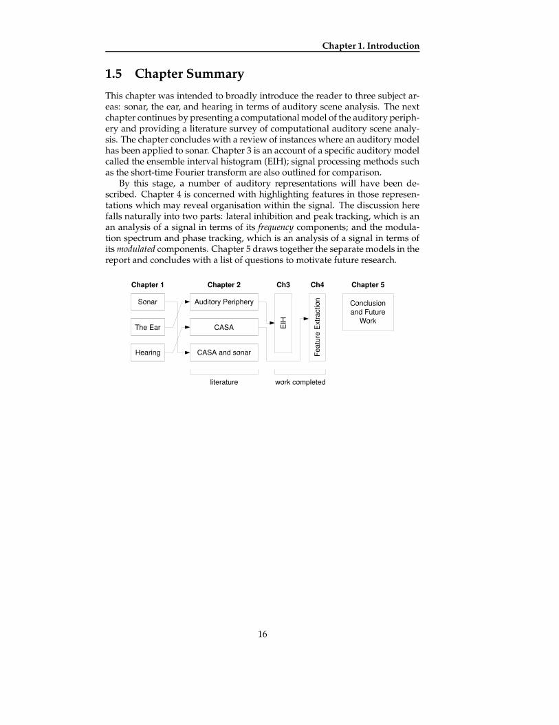
This chapter was intended to broadly introduce the reader to three subject ar-eas: sonar, the ear, and hearing in terms of auditory scene analysis. The nextchapter continues by presenting a computational model of the auditory periph-ery and providing a literature survey of computational auditory scene analy-sis. The chapter concludes with a review of instances where an auditory modelhas been applied to sonar. Chapter 3 is an account of a specific auditory modelcalled the ensemble interval histogram (EIH); signal processing methods suchas the short-time Fourier transform are also outlined for comparison.
By this stage, a number of auditory representations will have been de-scribed. Chapter 4 is concerned with highlighting features in those represen-tations which may reveal organisation within the signal. The discussion herefalls naturally into two parts: lateral inhibition and peak tracking, which is anan analysis of a signal in terms of its frequency components; and the modula-tion spectrum and phase tracking, which is an analysis of a signal in terms ofits modulated components. Chapter 5 draws together the separate models in thereport and concludes with a list of questions to motivate future research.
16

Chapter 2
Auditory Modelling
The preceding chapter provided a introduction to audition from two perspec-tives, namely, the physiology of the ear and the psychology of hearing. Thischapter examines previous attempts to find a computational analogue for these:a simulation of the auditory periphery is presented as a model of the ear, thenvarious systems for computational auditory scene analysis are introduced asmodels of hearing. The chapter concludes with a survey of auditory modelsand CASA systems used in sonar applications.
2.1 Modelling the Auditory Periphery
Models of auditory periphery attempt to capture the initial stages of processingin the auditory pathway, specifically, the filtering properties of the outer andmiddle ear, the motion of the basilar membrane, and the transduction of basilarmembrane motion to neural activity by the inner hair cells.
2.1.1 The Outer and Middle Ear Filter
For a moderate sound intensity, the combined resonances of both the outer andmiddle ear can be modelled by a linear transfer function, which pre-emphasisesfrequencies in the 2-4kHz region. In practice, this can be implemented in thetime domain by initially passing the signal through a high-pass filter, such as(43 �65�7� 3 �658*:9<; =?>#� 3 ��*@�A5 (2.1)
where � 3 �65 and (43 �65 are the respective input and output time series. Alterna-tively, the transfer function may be applied in the frequency domain by ad-justing the gain at the output of each auditory filter to match the shape of itsmagnitude response. It should be noted that these resonances appear to beappropriate for the efficient transmission of speech-like signals; in the case ofsonar, it may be advisable to omit this stage altogether.
2.1.2 Basilar Membrane Motion
Arguably, the most important processes of the auditory periphery are the filter-ing mechanisms of the basilar membrane. Typically, these are realised compu-
17
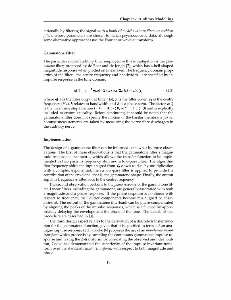
Chapter 2. Auditory Modelling
tationally by filtering the signal with a bank of model auditory filters or cochlearfilters, whose parameters are chosen to match psychoacoustic data, althoughsome alternative approaches use the Fourier or wavelet transform.
Gammatone Filter
The particular model auditory filter employed in this investigation is the gam-matone filter, proposed by de Boer and de Jongh [7], which has a bell-shapedmagnitude response when plotted on linear axes. The frequency domain prop-erties of the filter—the centre-frequency and bandwidth—are specified by itsimpulse response in the time domain,�������B� C2D!EGF0H�I%��*��#�%JK���<-0/?�L�"���%$NMA�!�PO�� Q������ (2.2)
where �4����� is the filter output at time � (s), R is the filter order, $ M is the centrefrequency (Hz), J relates to bandwidth and O is a phase term. The factor QS�����is the Heaviside step function ( Q������T�9<U��WV79 ; Q�������X�?U��WY79 ) and is explicitlyincluded to ensure causality. Before continuing, it should be noted that thegammatone filter does not specify the motion of the basilar membrane per se,because measurements are taken by measuring the nerve fibre discharges inthe auditory nerve.
Implementation
The design of a gammatone filter can be informed somewhat by three obser-vations. The first of these observations is that the gammatone filter’s magni-tude response is symmetric, which allows the transfer function to be imple-mented in two parts: a frequency shift and a low-pass filter. The algorithmfirst frequency-shifts the input signal from $#M down to d.c. by multiplicationwith a complex exponential, then a low-pass filter is applied to provide thecontribution of the envelope, that is, the gammatone shape. Finally, the outputsignal is frequency-shifted back to the centre frequency.
The second observation pertains to the phase response of the gammatone fil-ter. Linear filters, including the gammatone, are generally associated with botha magnitude and a phase response. If the phase response is nonlinear withrespect to frequency, the Fourier components become mis-aligned or phase-distorted. The output of the gammatone filterbank can be phase-compensatedby aligning the peaks of the impulse responses, which is achieved by appro-priately delaying the envelope and the phase of the tone. The details of thisprocedure are described in [3].
The third design aspect relates to the derivation of a discrete transfer func-tion for the gammatone function, given that it is specified in terms of an ana-logue impulse response (2.2). Cooke [6] proposes the use of an impulse-invarianttransform which proceeds by sampling the continuous gammatone impulse re-sponse and taking the Z-transform. By correlating the observed and ideal out-put, Cooke has demonstrated the superiority of the impulse-invariant trans-form over the standard bilinear transform, with respect to both magnitude andphase.
18

2.1. Modelling the Auditory Periphery
Gammatone Filterbank
A gammatone filter bank is an array of gammatone filters whose centres aredistributed over the frequency axis according to their bandwidth; the band-width, in turn, is a quasi-logarithmic function of frequency. The result is aseries of filters with overlapping passbands whose bandwidth and spacing in-creases at higher frequencies. Figure 2.1 shows the magnitude response of thefilters comprising a gammatone filterbank in the frequency domain.
500 1000 1500 2000 2500 3000−80
−70
−60
−50
−40
−30
−20
−10
0Filterbank Magnitude Responses
Frequency (Hz)
Atte
ntua
tion
(dB
)
Figure 2.1: The magnitude response of ten ERB-spaced gammatone filters.
2.1.3 Hair Cell Transduction
The hair cell transduction model of the auditory periphery generally receivesas input the simulated basilar membrane motion (e.g., from a gammatone fil-ter) and returns either a series of spike times or simply the average firing rate(spikes per second) or spike probability. The latter two choices are some-thing of a design compromise, as it is well-recognised that an average-raterepresentation does not account for all the information present in the audi-tory nerve. Nevertheless, models based on the average firing rate/probabilityhave successfully reproduced other phenenoma associated with the inner haircell transduction, most notably, spontaneous firing, saturation and adaptation(described later in this section), but also compression and phase-locking.
Meddis’ Hair Cell
One notable hair cell model is that of Meddis [14], which uses differential equa-tions to describe the transfer of transmitter substance between four interior re-gions of the hair cell: the factory, free transmitter pool, cleft and a reprocessing store(Figure 2.2). The physical significance of the equations can interpreted as fol-lows. Production begins at a factory, which is constantly1 releasing fluid intothe free transmitter pool Z ����� . From here, a fraction of the fluid [ ����� , which isrelated to the instantaneous amplitude of the signal, is released into the cleft.The amount of fluid in the cleft at a given time \ ����� governs the probability of a
1the production asympototically approaches a limit however.
19

Chapter 2. Auditory Modelling
Figure 2.2: Flow diagram and governing equations for the movement of trans-mitter chemical between IHC regions. Redrawn from Meddis (1986, Model Bfig. 10). [14]
spike being generated. Some of the transmitter in the cleft is lost (in proportionto ] ), but some is recycled via the reprocessing store (in proportion to ^ , � ).
The four stages of firing probability coincide with the absence, onset, du-ration and release of a stimulus, and can be explained within the context ofthe Meddis model. Prior to a stimulus, a hair cell generates a small numberof spikes owing to a leak from the transmitter pool into the cleft, which givesrise to spontaneous firing. When a stimulus is initially applied, the substance inthe transmitter pool ‘floods’ into, or saturates the cleft, causing a sharp rise inspike probability. Shortly afterwards, the probability drops as the fluid in thetransmitter pool is only replenished at the rate the factory can manufacture it.This change to a steady state is termed adaptation. Finally, when the stimulus isreleased, the spike probability drops to below the spontaneous firing rate (an-other form of adaptation), as the free transmitter pool is depleted. Eventually,the factory restores the cell to its resting state.
Other Approaches
There have been other attempts to model hair cell function by modelling thedepletion and replenishment of transmitter fluid between one or more reser-voirs. Besides these, there are a number of signal-processing alternatives. Sen-eff [21] uses a discontinuous function as a half-wave rectifier before applying aleaky integrator and low pass filter to mimic adaptation effects. Ghitza [9] usesa level crossing detector which implicitly achieves half-wave rectification andlogarithmic compression (see Chapter 3).
2.2 Computational Auditory Scene Analysis
Auditory scene analysis describes the role of the brain in segregating a mixtureof sounds into streams, which are likely to correspond to different sources inthe environment. ASA aids a listener in many aspects of everyday life, for ex-ample, in the separation of speech from a background of noise (including other
20

2.2. Computational Auditory Scene Analysis
speakers). Computational auditory scene analysis (CASA), by comparison, is theapplication of computer algorithms to accomplish the segregation of a mixtureof sounds using similar means to a human listener. A CASA system is typicallyimplemented in two stages. First, a model of the auditory periphery convertsa signal to an auditory representation, from which individual components areidentified. A second stage then reintegrates the components into streams onthe basis of auditory grouping principles, such as proximity, good continationand common fate.
The CASA model presented by Cooke [6] aims to separate the acousticsources in a mixture and is optimised, in certain aspects, towards the sepa-ration of speech signals from intrusive sounds. At the earliest stage, a gam-matone filter bank decomposes the signal into a series of narrowband channelsand the instantaneous frequency at each channel is estimated. Owing to theoverlap in auditory filters, harmonics and formants in the signal each have thepotential to drive a number of neighbouring channels, so that blocks of chan-nels or place groups respond at the same instantaneous frequency. As placegroups persist through time, they become synchrony strands—individual ob-jects within the auditory representation with quantitative properties, e.g. num-ber of channels covered, the average amplitude over those channels, variationin frequency, and so forth. These properties, among others, provide the evi-dence for regrouping the synchrony strands to form streams. Cooke also de-scribes an approach for resynthesising a signal from the synchrony strands,permitting an audible assessment of each stream.
A similar approach to CASA has been investigated by Brown [3] who hasdeveloped a model to separate sounds with particular attention to harmonic-ity and related changes in pitch. The auditory periphery stage closely followsthat presented in section 2.1. Rather than using synchrony strands, Brown’smodel computes autocorrelation and cross-correlation maps to identify periodici-ties within and across frequency channels. In addition to these, frequency transi-tion maps trace the motion of spectral dominances in the time-frequency plane,motivated by the discovery of modulation-sensitive neurons in the auditorynuclei. The coherent information obtained from the correlation, frequency-transition and onset-offset maps is used to create auditory objects, which aresubsequently grouped according to the grouping principles laid down by Breg-man.
Mellinger [15] has developed a data-driven CASA system for the separationof the instruments within a musical mixture, as opposed to speech. A musicalsignal clearly contains a rich variety of grouping cues: each note is associatedwith an onset and offset; pitched instruments produce a harmonic series; andrhythm and metre provide a temporal context—to name a few. The segregationof instruments within a musical piece is a formidable task however, consider-ing that most music is intentionally written so that harmonic series and onsetscoincide, i.e., instruments typically play notes of the same pitch (or at 3rd, 5thor octave intervals) at the same time. The early stage of the model extracts anumber of features from the signal in order to form auditory events, which arelater grouped to form streams. First, a model of the auditory periphery con-verts the input signal into a cochleagram, which encodes the neural firing rateat a given frequency and time. Using this representation, the derivative of aGaussian, or some suitable variant, is convolved with each channel to high-light peaks in the firing rate for each frequency and additional measures are
21

Chapter 2. Auditory Modelling
described to prevent onsets occurring when partials vary in frequency acrosschannels; offsets are detected using the same kernel, inverted in time. Fre-quency transition maps are obtained using an array of two-dimensional time-frequency filters, each of which responds to a particular change in frequency.Partials are initially grouped if their onsets coincide (small differences are toler-ated) and this grouping is subsequently reinforced or weakened over time ac-cording to correlations in frequency change. This means, for example, that twopartials can commence at the same time and be fused, but shortly afterwards beseparated owing to unrelated frequency changes. Conversely, partials whichstart at separate times are initially segregated and can later be grouped to-gether. This ability of the model to dynamically group and ungroup partialsmidstream models a psychological phenomenon known as hysteresis: the ten-dency for listeners to reinterpret an auditory scene on the basis of changingevidence.
The three CASA frameworks discussed thus far all have the common traitthat they are data-driven, that is, they group primitive elements within thesignal which exhibit some correlated properties, such as common onset andfrequency and amplitude variation. Ellis [8] has presented an alternative ap-proach, prediction-driven CASA, which makes use of prior knowledge in thesegregation process. The system makes moment-to-moment predictions of thewhat sound is about to follow based on an internal probability model; routinesignals will roughly follow this path of predictions, whereas a sudden devia-tion from the expected sound—a surprise—will force a reorganisation of theinternal state. Ellis’ prediction-driven architecture is a specific example of ablackboard architecture [12], which comprises four stages. The first of these isan auditory front-end, which consists of an onset map and a correlogram-basedperiodicity map, which are typical of the data-driven systems described earlier.The internal representation of a signal is formed from core representational el-ements, which are three generic categories of sound chosen for their distinctperceptual effect: transients, wefts (pitched signal), and noise clouds. The thirdstage is a prediction-reconciliation engine, which is responsible for formulatingpredictions on the basis of the internal state of the system and then reconcil-ing any differences between these predictions and observed input that follows.This is accomplished via a ‘two-way’ inference engine, in which hypothesesare formulated on the basis of evidence and hypotheses, in turn, explain otherevidence. The fourth stage is broadly defined as high-level abstractions and isan extensible set of rules to further constrain the inference engine, according toprior knowledge or data from other modalities.
Unoki et al. [28] have described a method for computational auditory sceneanalysis to segregate a signal from a noise background. The separation is pre-sented as an ill-posed inverse problem, the sources being two unknown quan-tities, and the observed signal being their sum. The problem can be then solvedby the application of constraints, derived from auditory principles. The initialfrequency analysis is performed by means of the discrete wavelet transform,using the gammatone as a mother wavelet. The output of each filterbank chan-nel [ , with centre frequency _a` , can be expressed in terms of functions of in-stantaneous amplitude b%` ����� and phase O ` � [ � .c ` �����d b!` �����2FAH2I���e _S` �%��efO ` ������� (2.3)
22

2.3. Auditory Modelling in Sonar
If it is known that there are two sources present, the observed signal at eachfilter [ may be written as the sum of two signals, indexed � , each associatedwith a magnitude gihij ` and phase k#hij ` :c ` �����d lhTm�n E j oqp gih�j ` �����2F0H�I���e _S` �!�re k#hij ` ������� (2.4)
Clearly, it is not possible to directly return to the constituent signals from theobserved sum alone, as there are an infinite number of solutions. Instead, theproblem is constrained using four of Bregman’s principles for auditory group-ing: onset and offset, gradualness of change, harmonicity and common fate.Gradualness of change is enforced by assuming that, over a short time win-dow, both amplitude and phase are a smooth function and can be representedby a low-order polynomial. Onsets and offsets are detected by the presence ofcoincident peaks in the channel envelopes, subject to some tolerance parame-ter. Whether to group two channels by common fate is decided on the basis ofthe correlation of their normalised envelopes.
2.3 Auditory Modelling in Sonar
In recent years, some have examined the possibility of applying auditory sceneanalysis techniques to sonar signals. This type of work can be approachedfrom two perspectives. The modeller may be interested capturing the listen-ing process of a human sonar operator who is aurally attending to the signal,a procedure which suggests confining the system to work with features thatare audibly appreciable to the operator. (Recall that operators rely on visualpresentations of the signal in addition to listening.) Alternatively, the studyof auditory scene analysis may influence the design of signal-processing al-gorithms, for example, to facilitate the grouping of signal components whichexhibit related changes. The latter approach is stated somewhat more flexiblyand permits a system to exploit characteristics of the signal which are imper-ceptible to humans.
There have been few instances of auditory-motivated sonar systems re-ported in the literature. Bregman’s book, Auditory Scene Analysis was first pub-lished in 1990 and, unsurprisingly, subsequent CASA research has primarilyproduced systems designed for speech or musical signals, as these are morefrequently the object of attention for ordinary listeners. Development has alsobeen motivated by prospects for improved technology in areas such as au-tomatic speech recognition and music transcription. Researchers in auditoryscene analysis have only recently turned their attention to sonar.
Teolis and Shamma [25] have presented a system for the classification oftransient events, which, while not concerned with auditory scene analysis (e.g.streaming) per se, is relevant to this study insofar as it investigated the meritsof using an auditory-motivated front end. The model first converted the in-put signal into the auditory representation, after which classification was per-formed by a feed-forward neural network. The representation was obtainedby taking the wavelet transform of the signal, a process akin to filterbank, inan effort to model cochlear filtering. This was followed by a partial differenta-tion with respect to both the time and filter index (the spatial axis), after which
23

Chapter 2. Auditory Modelling
a non-linear filter was employed to preserve only the extrema at each chan-nel and set all other values to zero. The output signals were then half-waverectified and smoothed over time to yield the final representation. The studycompared the auditory representation against a conventional power spectrumwhen used as input to the neural network, where a quantitative measure of per-formance was derived from the receiver operating characteristic (ROC) curve.The auditory representation consistently showed superior performance for anumber of signal-to-noise ratios and frequency resolutions.
Another system for the processing of transient events is the Hopkins Elec-tronic Ear (HEEAR) [18], which is implemented in analogue VLSI. Accordingly,the cochlear filters take the form of analogue bandpass filters and the hair-cell transduction is approximated using rapid adaptation circuit and a clipped,half-wave rectification. A feature vector is formed from the (smoothed anddecimated) output of each channel and then classified using a template-basedmethod. Recognising the difficulty of obtaining sonar transients in controlledconditions, the dataset used in the initial evaluation of the model was obtainedby striking objects in the laboratory. The classification of 221 transient eventsgave rise to 16 confusions between similar classes (e.g. claps and finger snaps).
A study conducted at the University of Sheffield [4] investigated the feasi-bility of event separation for sonar signals within the framework of the CASAarchitectures previously developed. In order to track the motion of multi-ple harmonics over time, the sonar signal was decomposed into synchronystrands: the auditory representation underlying Cooke’s CASA system. Re-sults were mixed: in severe noise conditions, poor estimates of instantaneousfrequency gave rise to many short strands, and transient events were not cap-tured; for cleaner recordings, harmonic content was represented well. Thestudy proceeded to examine the possibility of detecting transient events withinthe signal and then resynthesising a ‘transient-only’ stream. This was achievedby first detecting onsets, corresponding to a peak in the instantaneous ampli-tude across a contiguous block of filters. Having detected the peaks, the min-ima either side of each envelope peak were located and the intervening signalwas isolated as a transient. A final stage integrated the short transient signalsinto a continuous recording, after adjusting the signal envelopes to preventsharp discontinuities.
The next stage of the study concentrated on signal processing methods todecompose the signal into tonal, transient and noise components, such that thesum of the three would constitute the original signal. Similar procedures havealready been investigated using noise, sinusoids and transients as a representa-tion of a speech signal [13, 29]. The procedure for extracting the three signals isdescribed below and illustrated in Figure 2.3. An overlap-add analysis was ini-tially employed to divide the signal into short, windowed analysis frames, thenthe fast Fourier transform (FFT) of every frame was taken, resulting in a seriesof spectral estimates. With the signal in this form, the first step was to designateeach bin as tonal or not-tonal, which was accomplished using a peak-pickingalgorithm similar to the MPEG-1 criteria. Once it had been decided whichbins contained tonals, the overlap-add procedure was used to resynthesise thetonal signal from these bins alone; the remainder of the bins were resynthe-sised to give a residue of noise and transients. To separate the transients fromthe noise, the time-domain residual was transformed using the discrete cosinetransform (DCT)—the real half of the Fourier transform—to a frequency do-
24

2.3. Auditory Modelling in Sonar
Figure 2.3: Algorithm flow diagram for tonals, noise and transients model.
main representation, where spikes in the time-domain manifest themselves ascosine components. These cosine components were transformed by a furtherFourier transform creating peaks which could be detected and removed in thesame manner as the tonals, using the peak-picking procedure described above.A final resynthesis of the peaks (including the appropriate inverse transforms)created the transient stream; the remaining signal was labelled as noise. Pre-liminary experiments were performed aiming to classify (and visualise) tran-sient events by entering them into a multidimensional space, in which the axescorresponded to pre-elected spectral features. This procedure was rigorouslycarried out by Tucker using perceptually-motivated features and is discussedlater in this section.
Tucker [27] was the first to explore the benefits of using an auditory modelin the analysis of a reasonably large set of real sonar recordings and was chieflyconcerned with audible aspects of the signal. The first part of the study was apsychophysical experiment to examine the ability of a listener to infer the prop-erties an object (e.g. material, size and shape) by listening to the sound gener-ated when the object was struck, both in air and underwater. Submerged andin-air recordings were made for a number of struck objects, for which listenerswere asked to identify the size, shape and material. Estimates of shape and ab-solute size were poor, but the ratio in size between two objects was determinedmore accurately. When asked to assess the material of an object, wood andplastic were frequently confused, but metallic sounds were distinguishable.
The second stage of the study investigated the perceived quality or tim-bre of sonar transient events, such as knocks, clicks and chains. Tucker used amulti-dimensional scaling (MDS) technique to determine a perceptually-motivedfeature set which people used when classifying transients. Listeners were pre-sented with pairs of recordings and asked to rank their similarity on a scale.The scores were averaged over a number of trials and placed into a similaritymatrix. Subsequently, each recording instance was assigned a point in a three-dimensional space. The positions of these points were iteratively updated untilthe distances between them corresponded in an inverse fashion to the similar-ity matrix, so that ‘clusters’ of points represented sounds of a similar timbre.It should be noted that the distance between two points was determined ac-cording to the INDSCAL metric (as opposed to the Euclidean), which defines
25

Chapter 2. Auditory Modelling
and weights the axes in relation to individual subjects. The final step was tosearch for acoustic properties of the signal which were highly-correlated withthe dimensions of the multi-dimensional space. Results for sonar transientsindicated that the three dimensions correlated well with spectral flux, the fre-quency of the lowest-frequency peak and the temporal centroid.
In addition to transient events, sonar signals contain a rhythmic pulsating,which can be attributed to the revolution and configuration of a ship’s pro-peller; accordingly, a investigation into the temporal structure of sonar record-ings was undertaken. The rhythm of the sonar signal was assessed using therhythmogram [26]—a time-domain procedure which smooths the energy in thesignal at a number of scales, highlighting slow and rapid pulses. The overallrhythmic behaviour was summarised by obtaining an inter-onset interval his-togram (IIH) at each scale and pooling all the IIHs into a single feature vector.The resultant feature vector was rather long and redundant, so a number ofmethods for reducing the vector to a few salient values are described.
Kirsteins et al. [11] have produced a CASA-based model for the fusion ofrelated signal components within underwater recordings, which exploits corre-lated micromodulations in instantaneous frequency to group channels. In par-ticular, the system is capable of identifying the harmonic tracks within record-ings of killer and humpback whale vocalisations. However, it is questionablewhether listeners routinely group signal components on the basis of ampli-tude modulation and frequency modulation is not generally considered to bea strong grouping cue2. Arguably, the model would benefit from taking intoaccount more compelling grouping principles such as onset and harmonicity.
2.4 Summary
The majority of CASA research to date has concentrated on speech and mu-sic rather than sonar signals, which differ greatly in nature. Speech and musicare designed with a listener in mind, both in terms of the acoustic propertiesof the signal—its frequency and dynamic range—and the effective communi-cation of an idea, verbally or artistically. By constrast, the underwater soundsproduced by marine vessels are a precipitate and not intended to communicateinformation. Nevertheless, a vessel acoustic signature has a few audible prop-erties, which allow it to be described: a rhythmic pulsating, transient events,the shape of the noise spectrum and perhaps a weak sensation of pitch evokedby tonal components. Aspects of the signal that a human cannot hear must beinterpreted visually.
Tucker’s model is restricted to aspects of the signal which are directly au-dible, namely, rhythm and transients. Similarly, Teolis and Shamma’s model isconcerned only with transient events. Auditory models in sonar have tendedto neglect tonal components, which are not a striking feature in the recordingsbecause they are masked by noise and occur at low frequencies—although stillwell within an audible range. This is surprising, considering that conventionalCASA literature contains a wealth of techniques relating to the tracking andgrouping of frequency components in speech. The following chapters examine
2Although frequency modulation (FM) is not usually cited as a grouping cue per se, the ear isby no means deaf to FM. FM has an impact on the timbre of a sound and promotes grouping whenapplied as an extension of harmonicity.
26

2.4. Summary
auditory methods for the identification and organisation of tonal componentswithin a sonar signal.
27


Chapter 3
Time-FrequencyRepresentations and the EIH
The previous chapters have described how the structures of the cochlea—thebasilar membrane and inner hair cells—transduce a signal into a neural-spectralrepresentation. If a system is intended to perform the task of listening, then aprocess is required to emulate the signal-transforming action of the ear. Thischapter opens with an account of three signal processing techniques, whichmay be employed to model the signal in the auditory nerve to a first-order ap-proximation as a time-varying spectrum. Following this, a particular auditorymodel, the ensemble interval histogram, is presented as an alternative to theconventional spectrogram.
3.1 Signal Processing Solutions
3.1.1 Short-time Fourier Transform
The most popular choice of time-frequency representation is the short-timeFourier transform (STFT), which expresses the spectrum of a signal at a giventime from the Fourier transform estimated over a short window ������� either side.For a signal ������� , the (magnitude) STFT [20] is formally defined as:
cts!u ���qU _ �dwvvvvx@yD y ����z1�f��������z1� {?DG|�}�~'�?zavvvv
o(3.1)
The Fourier transform assumes that a signal is periodic, i.e. that it consists ofthe windowed signal repeated infinitely, so the window is typically taperedat each end (e.g. a gaussian, raised cosine or Hamming window) to preventsharp discontinuities occurring at the boundaries. The length of the windowhas implications for time and frequency resolution: a short window smoothsthe signal in the frequency domain; a long window smooths the signal in thetime domain. As far as is possible, the window is chosen to give adequate res-olution in both domains. What is considered adequate depends on the task inhand and the scale at which information is present in the signal. For speech,
29

Chapter 3. Time-Frequency Representations and the EIH
the window needs to simultaneously capture transient bursts in the time do-main, formant shape and pitch in the frequency domain, and pitch contoursin both; typically, a window length of 5ms–20ms is suitable. The detection oflow-frequency tonals in sonar requires a narrowband analysis.
3.1.2 Wigner Distribution
The Wigner distribution (WD) [20] is another joint time-frequency function,which is designed to address the resolution trade-off inherent in the STFT. Fora complex signal � ����� (where �<� denotes its complex conjugate), the WD at time� and radian frequency _ is defined as follows:c���� ���qU _ �d xPyD y {?D�|�}�~ � ���!�rz8�'�'� � � ���S*�z8�'�'���'z (3.2)
The Wigner distribution is able to precisely represent some analytically-definedmonocomponent signals such as exponentials, Dirac pulses, and frequency-sweeps in both time and frequency. In this case, the WD is the same as theSTFT with the windowing effect (i.e. averaging) removed. (In fact, convolvingthe WD of the signal with the WD of the window in two dimensions yields theSTFT spectrogram.) For certain signals, however, the WD suffers from artefactsarising from crossterms in the multiplication, to which the STFT is immune.Nevertheless, the Wigner distribution has been applied successfully in bothspeech and sonar [1].
3.1.3 Wavelet Transform
Within the last two decades, the wavelet transform (WT) has become widelyregarded as an alternative to the STFT. Rather than trying to remove uncer-tainty in time and frequency altogether, the WT emphasises each scale in sep-arate portions of the representation: good time resolution is obtained at high-frequencies; good frequency resolution is obtained at low frequencies. Initially,a mother wavelet or analysing wavelet, which often resembles a windowed sinu-soid, is used to filter the signal. This mother wavelet is then progressivelyscaled and dilated by powers of two, to produce output at further scales. Thecontinuous wavelet transform (CWT) is defined in terms of the mother wavelet�
, at time � and scale � :c ��u ���qU � �d �� ��� � � � x ������� � � � zt*,�� � �?z (3.3)
The WT has several desirable properties. First, a wavelet has the ability to lo-calise features in the time-frequency plane owing to its finite length, as opposedto a Fourier transform, which uses sinusoids of infinite duration. Second, theexponential scaling of the wavelets carves up the time-frequency plane so thatfrequency resolution is varied in a similar manner to the ear (see Figure 3.1).For this reason, the WT has been adopted by several workers in the auditorymodelling community as an approximation of the auditory periphery and ex-ploited in a number of sonar systems. [19, 25]
30

3.2. Ensemble Interval Histogram
Figure 3.1: The division of the time-frequency plane into cells by the STFT (left)and wavelet transform (right).
3.2 Ensemble Interval Histogram
This section describes the ensemble interval histogram (EIH) as an auditory mo-tivated method of spectral analysis. Here the frequency content of the signalis estimated from the spiking behaviour of simulated auditory-nerve fibres,producing a frequency-domain representation similar to a Fourier magnitudespectrum. A study conducted by Ghitza [9] has compared the performance ofa spoken digit recogniser for a variety of signal-to-noise ratios using featuresextracted from both the Fourier and EIH spectrum. The performance of theEIH-based system degrades less rapidly as the signal-to-noise ratio decreases,indicating the superior ability of the EIH to preserve harmonic structure in thepresence of Gaussian noise. The ability of the EIH to suppress noise makes ita candidate for the analysis of vessel acoustic signatures, considering the tonalcomponents—which may reveal the identity of a target—are often obscuredby a background of broadband noise sources. The remainder of this sectionassesses the suitability of the EIH as a front-end to a sonar classifier.
3.2.1 Model
The ensemble interval histogram is generated by applying three transforma-tions to the input signal. The first two of these correspond, in an abstract fash-ion, to the motion the basilar membrane and the transduction of this motioninto spiking activity by the inner hair cells. The third transformation is morespeculative, and pertains to the analysis of frequency in the auditory nerve.This section specifically describes the algorithm proposed by Ghitza; the over-all model is illustrated schematically in Figure 3.2.
The initial stage of the model consists of a bank of bandpass filters to simu-late the vibration of the basilar membrane, each filter output corresponding tothe motion at a given point. Specifically, the filter bank comprises eighty-fiveoverlapping cochlear filters, which are spaced logarithmically between 200Hzand 3200Hz to suit the frequency range of speech signals. Consistent with thepower spectrum model presented in section 1.3.1, the bandwidths of the filtersbecome wider with increasing frequency. Consequently, individual harmonicsare resolved by narrow filters at low frequencies, whilst at higher frequencies,a number of harmonics may interact under the passband of a single filter. Tem-poral resolution varies in the opposite sense: sudden onsets register quickly athigh-frequency filters; at lower frequencies, filters take a while to respond and
31

Chapter 3. Time-Frequency Representations and the EIH
Figure 3.2: Schematic illustration of EIH adapted from [9].
produce a smoother output.The next stage of the model assumes a population of inner hair cells for each
point along the basilar membrane. To implement this, a multi-level crossingdetector is assigned to each filter to transform the output from a sampled sig-nal into a series of spike events. Each positive-going level crossing represents acell being depolarised and the distribution of levels is chosen to reflect the vari-ability of inner hair cell thresholds. Ghitza assigns seven level crossings to eachchannel according to a number of Gaussian distributions whose means are dis-tributed logarithmically over the positive half of the signal, which accounts forboth dynamic compression and natural variability. It should be emphasisedthat only positive, positive-going crossings generate a spike, as depolarisation ofhair cells only occurs in a single direction.
The final stage of the model is a fine-grained frequency analysis of eachspike train: 595 in number, assuming eighty-five filters and seven level cross-ings. For a narrow band dominated by a near-sinusoidal stimulus, spikes willoccurs at regular intervals corresponding to the period of the signal and soconvey frequency-related information. For example, a 200Hz sinusoid cap-tured under a filter will produce a spike every 5ms. An interval histogram isformed by taking the reciprocal of the intervals to estimate frequency and pool-ing them over a short time frame into a histogram. To continue the previousexample, the 5ms intervals will be converted to units of frequency, i.e. 200Hz,and appear as a spike in the histogram. The ensemble interval histogram is thenobtained simply by summing all the histograms together. Ghitza’s histogramconsists of one hundred bins linearly-spaced over the range 0Hz–3200Hz anduses the twenty most recent intervals in each spike train. Some implications ofthis policy are discussed in the next section.
3.2.2 Properties
The ensemble interval histogram representation has some properties whichdistinguish it from a conventional spectrum. This section introduces three gen-eral properties, which relate to frequency resolution, noise robustness and time
32

3.2. Ensemble Interval Histogram
Figure 3.3: Two sinusoids with frequencies of 20Hz and 24Hz beating againsteach other for one second. Notice the resulting 4Hz period, which would beencoded by a high-threshold level-crossing detector.
0 1000 2000 3000
EIH
Out
put
Frequency (Hz)
Unresolved Harmonics
0 1000 2000 3000Frequency (Hz)
EIH
Out
put
Resolved Harmonics
Figure 3.4: left plot: unresolved harmonics at 2200Hz, 2300Hz, 2400Hz and2500Hz, causing a 100Hz ‘fundamental’ spike; right plot: resolved harmonicsat 100Hz, 200Hz, 300Hz and 400Hz.
resolution; discussion of their implications for sonar are postponed to section3.2.4.
The frequency-dependent resolution of the EIH can be attributed princi-pally to the filterbank stage, in which the bandwidth and separation of thefilters increases with frequency, causing harmonic components to be encodeddifferently at each end of the spectrum. This is best understood in terms of theanalysis of a harmonic series. For example, for a series with a 100Hz funda-mental, the first few harmonics are captured under narrow filters and so ap-pear in the EIH as distinct spikes at 100Hz, 200Hz and so on. High-frequencyfilters have bandwidths wider than the fundamental and can therefore containmultiple harmonics, which cannot be individually resolved. Instead, the par-tials appear in the EIH as a mass of high-frequency energy. As a secondary ef-fect, the interaction between two partials gives rise to a beating in the envelopeof the filter output at their frequency difference, which is picked up by level-crossing detectors and is encoded as a low-frequency spike in the EIH. Figure3.3 demonstrates how the EIH encodes the frequency difference between un-resolved partials and Figure 3.4 shows actual EIH output for select groups ofpartials.
The suppression of noise within the EIH is achieved in two ways. The firstof these is the overlap in the passbands of the cochlear filters. When a fre-quency component has sufficient amplitude, it can dominate the output of afew filters with centre frequencies close to the stimulus, each of which then
33

Chapter 3. Time-Frequency Representations and the EIH
Figure 3.5: Temporal response of the EIH. The time of analysis is indicated bya dashed line, the bars indicate the time over which the histogram is formed ineach channel (only past values are used).
contributes to a peak in the ensemble interval histogram. Noise suppression isassisted further by the the formation of an interval histogram. A conventionalspectrogram divides energy into frequency bins and each bin communicatesonly the magnitude (and phase) of its content—there is no way of determin-ing to what extent the bin contains tonal or noise energy. By constrast, thecontent of an interval histogram reflects the nature of the stimulus within asingle band: a tonal gives rise to regular intervals, contributing to single binof the histogram; noise produces varied intervals and so gets ‘spread’ over thehistogram.
The time resolution of the EIH varies with frequency, the best resolutionbeing achieved at high frequencies1. This can be attributed in part to the fil-terbank configuration, whose high-frequency filters are associated with bettertemporal resolution. The principal factor, however, is the choice of a constantnumber of intervals per histogram. The reciprocal relationship between fre-quency and interval duration implies that a fixed number of low frequencyintervals will span a longer time than the same number of intervals at a higherfrequency. For example, 20 intervals at 10Hz will cover 2 seconds but 20 in-tervals at 100Hz will cover only 0.2 seconds. In this sense, the time-frequencytrade-off of the EIH may be likened to a wavelet transform: spectral and tem-poral features are well-defined in the low- and high-frequency portions of thespectrum, respectively. It is of course possible to even the time resolution byappropriately scaling the histogram ranges, but taking fewer intervals at low-frequency channels would incur a loss in frequency resolution.
3.2.3 Analysis of Vowels
A model has been developed in MATLAB to generate an EIH-based spectro-gram, which takes the form of an image showing the energy in the EIH as itchanges over time. It is therefore a time-frequency representation derived fromthe EIH, just as a conventional spectrogram is derived from the Fourier trans-form. Before progressing to sonar signals, a preliminary investigation com-pared the two types of spectrogram for some artificial vowel sounds, both cleanand mixed with Gaussian noise. The vowel sounds examined were those usedin Summerfield and Assmann’s double-vowel experiment [24]: each has a du-
1assuming a high sample rate—see section 3.2.5.
34

3.2. Ensemble Interval Histogram
Time (s)
Freq
uenc
y (H
z)
(a) EIH CLEAN
0.05 0.1 0.15 0.20
1000
2000
3000
Time (s)
Freq
uenc
y (H
z)
(b) EIH NOISY
0.05 0.1 0.15 0.20
1000
2000
3000
(c) FFT CLEAN
Time (s)
Freq
uenc
y (H
z)
0 0.05 0.1 0.15 0.20
1000
2000
3000
(d) FFT NOISY
Time (s)
Freq
uenc
y (H
z)
0 0.05 0.1 0.15 0.20
1000
2000
3000
Figure 3.6: Spectrograms for vowel sound /ER/. Top-left: clean EIH; top-right:noisy EIH; bottom-left: clean FFT; bottom-right: noisy FFT.
ration of 200ms and consists of a harmonic complex, shaped by a filter to createformant peaks. The parameters of the EIH were chosen to closely match thoseof Ghitza’s model, although random variability in the level crossings was omit-ted for the sake of economy. The filtering stage was accomplished by a gam-matone filterbank, whose centres and bandwidths were chosen according toequivalent rectangular bandwidth. The original vowel sounds had a sample-rate of 10kHz but were upsampled to 50kHz for the EIH, which requires a finertime resolution for level crossing estimates.
This section examines the EIH and FFT spectrogram for a single vowelsound, /ER/, with a fundamental frequency of 100Hz and formants at 450Hz,1250Hz and 2650Hz. In the clean EIH-spectrogram, the first formant is re-solved by the narrow, low-frequency filters into five constituent partials—thefundamental and the four lowest harmonics. The next two formants appear inthe EIH as thick bands, as the filters at higher frequencies are too wide to cap-ture individual partials. The EIH was recalculated for the same signal mixedwith additive Gaussian noise at 0dB (with respect to RMS) to produce Fig-ure 3.6(b). The harmonics of the first formant remain clearly visible and thesecond formant (1250Hz) is still discernable but somewhat intermittent. Thethird, weaker formant (2650Hz) is lost completely, owing to the poor frequencyresolution of the wide filters. FFT-based spectrograms of the vowel soundswere generated with a frame-length and frame-shift designed to give compa-rable time-frequency resolution to the EIH. The results for the clean signal aredepicted in Figure 3.6(c), and the noisy signal in Figure 3.6(d). In the noise-free case, the individual harmonics within the signal are all visible, appearingas horizontal stripes; the darker/redder patches indicate formant regions. Inthe noisy spectrogram, the low frequency harmonics are still visible above thenoise but the second and third formants are obscured.
35

Chapter 3. Time-Frequency Representations and the EIH
FFT SPECTROGRAM
Frequency (Hz)
Tim
e (s
)0 200 400 600 800 1000
0
1
2
3
4
EIH SPECTROGRAM
Frequency (Hz)
Tim
e (s
)
0 200 400 600 800 1000
0
1
2
3
4
Figure 3.7: Spectrogram (top) and EIH (bottom) for four seconds of sonar.
3.2.4 Analysis of Sonar
A vessel acoustic signature has already been presented as a combination ofnarrowband and broadband components, the former providing the most use-ful features for classification. Application of the ensemble interval histogramto a sonar signal may highlight tonal structure buried within noisy portions ofthe spectrum, much in the same way as the higher formants of the vowel signalwere preserved. Figure 3.7 shows both a conventional and EIH-based spectro-gram for a four-second clip of a vessel recording. In the first instance, the EIHparameters were chosen to be identical to the vowel experiment (85 filters and7 level crossings), the only notable exception being that the filters were spacedupto 1kHz to provide coverage of a relevant frequency range. The EIH wasgenerated every 50ms, resulting in eighty frames over the four seconds.
A number of harmonically-related tonals are apparent in the FFT-basedspectrogram, especially at frequencies lower than around 500Hz, where thecrossover point occurs. The spectrum is dominated by noise above this fre-quency, although some tonal components are vaguely evident. The corre-sponding EIH-based spectrogram poorly represents the content of signal: ona broadband scale, the spectral energy appears to agree with the FFT, but thediscrete lines are no longer visible and artefacts are present at higher frequen-cies. The following sections discuss the cause of these problems and suggestsome adaptations to the EIH algorithm to ensure a more faithful encoding ofthe signal.
Filterbank Configuration
The initial stage of processing within the EIH is a gammatone filterbank (orsome similar implementation), which decomposes the signal into narrow bands.
36

3.2. Ensemble Interval Histogram
Figure 3.8: Proposed redistribution of gammatone filters for a sonar applica-tion.
So far, the logarithmic spacing of the filters has been emphasised as a key fea-ture of the model. However, given that we are interested in identifying tonalcomponents across a range of frequencies, it is reasonable to question the jus-tification for this spacing, which results in poor frequency resolution in theupper-half of the spectrum—especially considering that most of the noise isconcentrated in this region. By contrast, a bank of narrow, linearly-distributedfilters would offer uniform frequency coverage as illustrated in Figure 3.8. Ar-guments for the logarithmic spacing originated from a concern to model au-ditory function, but there remain valid arguments for a linear spacing. First,auditory filters are spaced linearly at frequencies under 1kHz anyway and onlystart spreading out at higher frequencies. Second, it may be contended that thepurpose of wide high-frequency filters is to aid the perception of pitch via theinteraction of unresolved harmonics, not partials. Third, it is possible that poorfrequency resolution is a deficiency—the best the ear can achieve given themechanical properties of the basilar membrane and phase-locking capacity ofnerve cells. For these reasons, a linear spacing of filters has been adopted. Itshould be noted, however, that the overlap between filters has been retained.
Level-crossing Thresholds
The constrast of spectral components within the EIH depends crucially uponthe choice of level crossing amplitudes. If the level-crossing thresholds are toosensitive, then energy will appear in the EIH wherever there is noise. On theother hand, if the thresholds are set too high, then genuine components maynot be represented at all, which appears to be the case in Figure 3.7. The de-fault method for choosing level-crossings so far has been to find the maximumabsolute peak over all channels and designate this as the highest threshold, asshown in Figure 3.9(a). However, taking the maximum value as an indicatorof the dynamic range is inappropriate, as a tonal or transient event with a highamplitude can result in genuine features failing to register. Calculating themean energy over all the channels is an improved strategy, but a strong tonal ortransient still has the potential to offset the mean, causing the same problem,only less severe—see Figure 3.9(b).
The methods described so far have operated on the assumption that level-crossings should be uniform for all channels. This assumption is invalid forsonar spectra, in which tonal levels vary, particularly between noisy and noise-free regions of the spectrum. Selecting thresholds based on the maximum (ormean) energy for each channel independently of the others is a considerationthat may be readily dismissed, as tonal features will no longer be distinguish-able (see Figure 3.9(c)). Instead, the method adopted is to remove the trendin the spectrum by choosing levels according to a polynomial fit through themean channel output, counteracting the effects of the broadband component.
37

Chapter 3. Time-Frequency Representations and the EIH
The order of the polynomial dictates the smoothness of the trend: a linear orquadratic function appears to work well. Figure 3.9(d) shows the thresholdsfor a linear fit through the spectral energy.
The inclusion of these two modifications—spacing the gammatone filterslinearly and adjusting the thresholds using a polynomial fit—results in fargreater detail in the EIH spectrum for a sonar signal. The modified algorithmwas used to produce the EIH spectrogram in Figure 3.10.
3.2.5 Using Entropy and Variance
Previous studies have shown that the average firing rate of cells within theauditory nerve cannot solely account for all the audible properties of a sig-nal and that it is likely that further information is encoded by temporal dis-charge patterns. The EIH model converts a signal into spiking activity usinglevel-crossing detectors; from here, a mechanism is required to abstract usefulproperties from the spike trains. Ghitza’s model forms a representation di-rectly from the inter-spike intervals but it is also conceivable that order withinthe spikes conveys salient information about the quality of the stimulus excit-ing the model cell, e.g., tonal or noise. Two measures of order are proposedhere: entropy and variance, both of which are properties of probability distri-butions. To find the entropy of a spike train, a histogram is formed for eachchannel over a short time window, this histogram is used to estimate a proba-bility distribution � , and then the entropy � for each channel is obtained fromthe distribution � |S� � . � � � �d�*�l�0����� � |#� /'� � | (3.4)
By dividing the spike train into frames and computing the entropy in eachchannel, it is possible to express the randomness of a signal as a function offrequency and time. Similarly, the variance of the spike intervals encodes thetype of stimulus: clean tonal components are associated with a low intervalvariance. The variance � can be calculated directly from a sample of intervals� | of size � and mean �� using:
� �� *����l | m E ��� | * ���� o (3.5)
Figure 3.9: Assigning levels based on: (a) maximum energy; (b) mean energy;(c) individual energy; (d) linear fit.
38
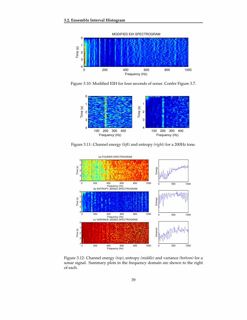
3.2. Ensemble Interval Histogram
MODIFIED EIH SPECTROGRAM
Frequency (Hz)Ti
me
(s)
0 200 400 600 800 1000
0
1
2
3
4
Figure 3.10: Modified EIH for four seconds of sonar. Confer Figure 3.7.
Frequency (Hz)
Tim
e (s
)
100 200 300 400
0
1
2
3
4
Frequency (Hz)Ti
me
(s)
100 200 300 400
1
2
3
4
Figure 3.11: Channel energy (left) and entropy (right) for a 200Hz tone.
(b) ENTROPY−BASED SPECTROGRAM
Frequency (Hz)
Tim
e (s
)
0 200 400 600 800 1000
0
1
2
3
4
(c) VARIANCE−BASED SPECTROGRAM
Frequency (Hz)
Tim
e (s
)
0 200 400 600 800 1000
0
1
2
3
4
0 500 1000
Ent
ropy
0 500 1000
Var
ianc
e
0 500 1000
Ene
rgy
Frequency (Hz)
Tim
e (s
)
(a) FOURIER SPECTROGRAM
0 200 400 600 800 1000
0
1
2
3
4
Figure 3.12: Channel energy (top), entropy (middle) and variance (bottom) for asonar signal. Summary plots in the frequency domain are shown to the rightof each.
39

Chapter 3. Time-Frequency Representations and the EIH
Figure 3.13: A crossing time derived from a linear fit (dotted line) between twosamples of a sine wave (solid line).
The result of plotting entropy in the time-frequency plane is shown in Fig-ure 3.11 for a 200Hz tone in noise (at 10dB SNR wrt. RMS), alongside the logenvelope in each channel. The entropy encodes the presence of the tonal bythe order it creates in the spike pattern; the log envelope displays energy butdoes not specifically distinguish a tonal from noise. Figure 3.12(a) shows thespectrogram of a sonar recording alongside the channel entropy 3.12(b) andvariance 3.12(c). It should be noted that tonals are associated with a low in-terval entropy and variance and so are manifested as sharp ‘troughs’ in thesummary plots. (However, the colour map is reversed in the images for con-sistency with the spectrogram.) Three immediate observations may be maderegarding the output: first, for all three means of detection, tonals are repre-sented in the lower 500Hz portion of the spectrum; second, variance appearsto affect individual filters, whereas a high-energy tonal (such as 150Hz) affectsentropy in many bands; and third, artefacts have appeared in the upper regionof the entropy plot (i.e. evidence of tonal components where there are none).These artefacts can be attributed to poor level-crossing estimates; the next sec-tion suggests ways to remedy this problem.
Improving Level-crossing Estimation
Frequency estimates are formed from the reciprocal of the interval time, so itis clear that accurate crossing times must be obtained to avoid severe errorsin the frequency measurement. For example, 1ms measured as 0.99ms willchange the frequency estimate from 1000Hz to 1010Hz, which is a significanterror. In general, level crossing times are difficult to obtain with this degree ofprecision due to the sampled nature of the signal. A straight-forward imple-mentation detects when two points fall either side of a crossing threshold, thenuses a linear fit between the points to estimate the crossing. However, in the re-gions of a sinusoid where the curvature is greatest (i.e. the peaks and troughs),a linear fit can result in considerable error, as depicted in Figure 3.13. High-frequency channels are particularly vunerable to this type of error, as there arefewer samples per signal period. The entropy at high frequencies in Figure3.12(b) is sensitive to the channel frequency: whenever the CF is misalignedwith the sample rate, a form of ‘beating’ occurs and introduces artificial vari-ance into the intervals, which is interpreted as randomness; however, whenthe samples are aligned with the CF period, this variance is absent. In order tocounteract this effect, it is necessary to better estimate the crossing times. Thiscan be achieved by fitting a polynomial through a number of samples (e.g. acubic spline interpolation), or alternatively, the entire signal can be upsampled.
40

3.3. Summary and Discussion
UPSAMPLED ENTROPY−BASED SPECTROGRAM
Tim
e (s
)
Frequency (Hz)0 200 400 600 800 1000
0
1
2
3
4
0 500 1000
Ent
ropy
Figure 3.14: Channel entropy for an upsampled sonar signal.
Figure 3.14 shows the channel entropy for the same signal, upsampled by a fac-tor of three. The high-frequency spikes have disappeared but the channel CFstill appears to have a slow-varying influence on the entropy.
3.3 Summary and Discussion
This chapter has outlined the key properties of the EIH as a time-frequencyrepresentation and presented some sample output for a sonar signal. One ofthe properties that may be considered undesirable in a sonar application is theencoding of the envelope modulation as a low-frequency component, which isexplained in section 3.2.2. This means, for instance, that two high-frequencypartials separated by 100Hz will give rise to an additional 100Hz componentin the EIH. The alternative design proposed for the sonar signals uses narrowfilters at high-frequencies and will therefore cause fewer interactions. The po-tential remains, however, for two components to interact within individual fil-ter channels. For this reason in particular, it is not advisable to directly replaceFFT-based spectrograms with the EIH. Instead, the EIH should be treated as aseparate form of representation, which characterises both frequency and pitcheffects.
The entropy and variance based methods have shown promise in provid-ing an alternative perspective of the signal, by quantifying noise rather thanenergy, although some work remains to be done in refining the algorithm toavoid artefacts. It should also be noted that the entropy-based EIH does notproduce tonals whose heights correspond to the magnitude in an FFT, so thisapproach cannot be directly applied to obtain spectra for classification. Never-theless, there is an argument for adopting these methods to detect the locationof tonals; the amplitude can be subsequently determined from the envelope inthose channels.
41


Chapter 4
Feature Extraction
This chapter discusses a number of ways in which features within a sonar sig-nal may be extracted. The signal representations presented in the previouschapter all produced a decomposition of the signal energy (or variance) in thetime-frequency plane; our attempts to model audition have only extended asfar as the auditory periphery. Four high-level analyses of a signal are now de-scribed: the first and second of these, lateral inhibition and peak detection, discussthe enhancement and tracking of frequency components through time. Thethird section presents the modulation spectrum, which allows a signal to be char-acterised in terms of spectral and amplitude modulations. The fourth sectionis concerned with the phase of frequency components; specifically, whethercommon fluctuations in phase can be used to group components by source.
4.1 Lateral Inhibition
It has long been recognised that cells within the auditory and visual appara-tus are assembled in such a way that activity in one region of cells tends toinhibit the response of adjacent regions, a phenomenon known as lateral inhi-bition. Visual scenes are encoded across the retina and optical nerve, so lateralinhibition serves to accentuate edges and suppress areas of uniform intensity.This is effectively illustrated by the Hermann grid in Figure 4.1. Similarly, au-ditory stimuli are encoded in a tonotopic, frequency-ordered fashion (it is in-structive to consider the response over a cross-section of the auditory nerve asa ‘snapshot’ of the spectrum) so lateral inhibition sharpens spectral edges andweakens contiguous regions of activity, e.g. broadband spectral features.
Figure 4.1: The ‘Hermann grid’ optical illustion—note the illusory grey patchesat the intersections of the white bands.
43

Chapter 4. Feature Extraction
The effective detection of and measurement of tonal components within asonar signal has already been emphasised as a key factor in the performance ofmachine classifiers. In modern sonar systems, tonal components are enhancedusing a strategy quite similar to lateral inhibition called spectral normalisation.[30] Spectral normalisation is accomplished by estimating how much energy inan FFT bin arises from broadband components, typically by averaging the en-ergy in bins a short distance either side, and simply removing this contributionby subtraction. The remainder of this section progresses toward a computermodel lateral inhibition which uses short-term association to highlight tonalcomponents within a signal.
4.1.1 Shamma’s Lateral Inhibition Model
Shamma has developed a lateral inhibition network (LIN) [22] to simulatethe response of a group of individual artificial neurons, which are linked byweighted inhibitory connections. Shamma has formulated two topologies forthe LIN: recurrent and non-recurrent.
The recurrent LIN consists of two layers. The first layers serves merely asan input buffer (in the same way as a a multilayer perceptron). The secondlayer consists of units whose input-output relation is given by the differentialequation in (4.1), where
c ����� and ����� respectively stand for the input andoutput at time � . This function causes the unit to charge and discharge slowlylike a capacitor, as shown below.
z � ������?� � ����� c ����� (4.1)
There are two sets of connections between the units: ¡ ��eKU6¢�� which connect unite in the first layer to unit ¢ in the second layer, and £ ��eKU�¢2� which connect unitse and ¢ in the second layer to each other. The governing equation for an outputunit | is expressed mathematically as (4.2) and diagramatically as Figure 4.2.
z � |�?� � | l#¤ ¡ ��eKU6¢�� c | * lN¤ £ ��eKU�¢2� | (4.2)
The non-recurrent LIN is formulated almost in the same manner as the re-current: the first layer is a buffer, the second layer consists of units with thesame activation function. The key difference is that there is no inhibitory feed-back between the output units; instead, the output of the each unit is calculatedindependently of every other (4.3) before the inhibitory weights are appliedover the layer to give a third output layer ¥ | (4.4). The non-recurrent LINtopology is illustrated in Figure 4.3.
44

4.1. Lateral Inhibition
Figure 4.2: Recurrent LIN.
Figure 4.3: Non-recurrent LIN.
z � |�?� � | l ¤ ¡ ��eKU�¢2� c | (4.3)
¥ | | * l ¤ £ ��eKU�¢2� | (4.4)
So far, the layers in both LINs have been described in terms of discretearrays of units. Rather than considering individual units
c | , | and ¥ | , inwhich e takes integer values, it is useful to form each layer from a continuumof units ����¦§� , ( �"¦N� and � ��¦N� as a function of the continuous variable ¦ . If theconnectivity of the units is symmetric and homogeneous then the interactionacross the weights can be interpreted as a spatial convolution ( ¨ ). Taken in thelimit, the equation for the recurrent LIN becomes (4.5):z � ( �"¦?U�����'� � ( �"¦?U����d ¡ �"¦N� ¨ ���"¦?U����S* £ ��¦§� ¨�( �"¦?U���� (4.5)
and the equations for the non-recurrent LIN become (4.6) and (4.7):
z � ( �"¦?U�����'� � ( �"¦?U����© ¡ �"¦N� ¨ ����¦?U���� (4.6)� �"¦?U����ª ( �"¦?U����a* £ ��¦N� ¨�( �"¦?U���� (4.7)
45

Chapter 4. Feature Extraction
0 2k (rads)
Mag
nitu
de
REC V(k)=1
0 2k (rads)
Mag
nitu
deNON−REC V(k)=1
0 2k (rads)
Mag
nitu
de
REC V(k)=lowpass
0 2
Mag
nitu
de
k (rads)
NON−REC V(k)=lowpass
Figure 4.4: LIN (linear) magnitude plots. Top-left: recurrent, no smoothing;top-right: recurrent, low-pass filtered; bottom-left: non-recurrent, no smoothing;bottom-right: non-recurrent, low-pass filtered.
Now the equations simply take the form of two filters, operating with respectto the spatial and temporal axes ( ¦ and � , respectively). The overall responseof the LIN can therefore be determined by the application of the Laplace trans-form to time—eliminating the differential term—and the Fourier transform tospace. The result is a spatio-temporal transfer function for the recurrent (4.8)and non-recurrent (4.9) LIN, in terms of � and [ , which are the complex vari-ables of the Laplace (time) and Fourier (space) transforms, respectively.
«�¬ � � U [ �© � � [ �z � �7���P�� [ � (4.8)« � ¬ � � U [ �© � � [ � 3 �W*r�� [ �f5z � �)� (4.9)
If a signal is slow-varying then the temporal integration can be disregarded bysetting z®�9 . This leaves a function purely in terms of [ , i.e. a spatial transferfunction. Both of these formulations describe a high-pass filter as shown inthe left-hand plots of Figure 4.4. The weights between the input and outputlayer, ¡ ��¦§� , act as a low-pass filter, averaging over neighbouring input units.The effect of including these weights is shown in the right-hand plots of Figure4.4, where high-frequencies have been attenuated somewhat.
4.1.2 Modelling Lateral Inhibition in MATLAB
Frame-based High-pass Cepstral Filter
A form of lateral inhibition can be applied to sonar signals in MATLAB by di-viding the signal into frames, taking the Fourier transform of each frame, andpassing each spectral slice through a high-pass filter, as both the recurrent and
46

4.1. Lateral Inhibition
non-recurrent LINs described in the previous section have a similar high-passcharacteristic; the filter used here is chosen to have zero-gain and represents aninhibitory lobe extending over two channels either side (4.10)—see Figure 4.5.Negative values which appear in the filtered spectrogram are set to zero.« � � �a791;���P9<; ¯ � D4E* � D o �P9<; ¯ � DG°d�P9<; � � D8± (4.10)
0 0.5 1 1.5 2 2.5 3−30
−20
−10
0
10
20
Atte
nuat
ion
(dB
)
Radians
Figure 4.5: Magnitude response of«
.
The results of this procedure, shown in Figure 4.6, are not particularly impres-sive; however two transients, which appear at 2 and 6 seconds as solid, hori-zontal lines, are diffused to some extent by the lateral inhibition.
Lateral Inhibition and Linear Association
Broadband transients can obscure a number of tonal tracks, especially at highfrequencies. In the second MATLAB model, the relationship between tonal com-ponents is tracked over time, so that when a tonal is briefly obscured, is canbe restored from surrounding evidence. The first stage of the model is a gam-matone filterbank, from whose channels the instantantaneous amplitude is ex-tracted as a changing spectral estimate. The spatial filter in (4.10) is then con-volved with the envelope to sharpen the spectral profile.
The next stage involves using the observed spectrum to form a weight ma-trix: a square matrix whose elements reflect the correlation between each chan-nel in the output. Such a matrix can be obtained by multiplying a columnvector containing the magnitude spectrum � by its transpose:g 7�³²0� uIn practice, the weight matrix A is continually refreshed by adding these ma-trices at each point in time; the rate at which observations are absorbed intothe weight matrix is determined by the coefficient ´ . At the same time, exist-ing correlations within the matrix decay exponentially, according to a decaycoefficient + . g ���%�)�N�d g �����%� ´�3 �������a²0������� u 58*�+ g �����The weight matrix is employed moment by moment to alter the content ofthe spectrum according to learned correlations. The observed spectrum at anyinstance is pre-multiplied by the latest weight matrix to give the output ������� :�������d g ����� �������
47

Chapter 4. Feature Extraction
Frequency (Hz)
Tim
e (s
)
SPECTROGRAM
0 200 400 600 800 1000
0
2
4
6
8
Frequency (Hz)
Tim
e (s
)
LATERAL INHIBITION
0 200 400 600 800 1000
0
2
4
6
8
Figure 4.6: Lateral inhibition for a sonar signal accomplished using a high-passspatial filter.
The overall purpose of the model is to gradually form correlations from in-stantaneous spectral estimates. When a broadband transient obscures one ormore tonals, the energy from the unaffected tonals is ‘passed’ back through theweight matrix, allowing partial restoration. This is in fact a form of smoothing,the temporal extent of which is dictated by ´ and + . This effect is vaguely rem-iniscent of the auditory continuity illusion described in section 1.4, in which atone is perceived to continue through a brief interruption. Two differences areworth mentioning, however: first, the continuity effect is only observed whenthe noise has sufficient energy to support the conclusion that the tonal has con-tinued through it; second, the continuity effect does not arise from tonals re-inforcing each other—the effect can be brought about by a single tone. Anillustration of the effect of lateral inhibition and linear assocation is shown inFigure 4.7: tonal components are generally more visible; transient events areless prominent.
It has been noted that this method only performs well under a limited setof circumstances, in particular, that the noise elements (transients and back-ground) have flat or smooth spectra. If the noise has a smooth spectrum, thenthe lateral inhibition stage removes the noise effectively; if however, there arepeaks in the noise spectrum, which is often the case, then lateral inhibitioncauses them to be accentuated. These artefacts then contribute to the weightmatrix and so remain in the output until they are removed by the exponen-tial decay. This specific problem highlights a more general deficiency of thisapproach: that the model sometimes produces features in the output, whichare not present in the input. The auditory continuity effect, on the other hand,does not suffer from this shortcoming because features are not induced wherethere is no energy to evidence their presence.
48

4.1. Lateral Inhibition
Frequency (Hz)
Tim
e (s
)
SPECTROGRAM
0 200 400 600 800 1000
0
1
2
3
4
Frequency (Hz)
Tim
e (s
)
LATERAL INHIBITION AND LINEAR ASSOCIATION
0 200 400 600 800 1000
0
1
2
3
4
Figure 4.7: Lateral inhibition network with linear association.
4.1.3 Discussion
Lateral inhibition can be summarised as a process that sharpens the discontinu-ities in an input pattern by reinforcing differences in intensity. This behaviouris defined locally: every active unit—a cell or an artificial neuron—suppressesthe response of its neighbours so that groups of active units are mutually in-hibitory. The response is maximal at the boundaries between active and inac-tive regions: here units are both excited by a stimulus and uninhibited fromone or more sides. Different formulations of a lateral inhibition circuit give riseto a variety of a high-pass spatial filters.
This section has discussed the possibility of using lateral inhibition in asonar algorithm for the enhancement of spectral features such as tonals. Onepractical drawback to using lateral inhibition is the potential for a strong tonalto exert such a powerful inhibition over adjacent frequency bins that any low-energy tonals in its locality are filtered entirely. One solution to this problemcould be a multi-staged lateral inhibition: a coarse first pass finds the tonalswith high energy and records their positions and magnitudes; these tonals arethen subtracted to leave a residual spectrum, which is subject to further passes.Another solution could be a multipath model, which uses lateral inhibitionat some stages and not others. For example, a high-pass spectral filter couldbe used to ‘sketch’ the frequency domain, allowing fundamental frequenciesto be identified and so on. This evidence could then be passed to a separatecomponent of the model to assist a fine-grained spectral analysis.
49

Chapter 4. Feature Extraction
4.2 Peak Detection and Tracking
The task of peak detection and tracking is of great relevance to both auditorymodelling and sonar technology. CASA models rely on peaks in the short-timemagnitude spectra, or a similar time-frequency representation, to trace the mo-tion of speech formants or musical notes, for example. Similarly, a passivenarrowband sonar analysis examines the amplitudes and frequencies of spec-tral peaks to identify a vessel. Isolating genuine peaks in noisy spectra can beproblematic, especially in the presence of a continuous noise spectrum, whereweak tonals are almost indistinguishable from the noise floor.
4.2.1 Time-frequency Filtering
The preceding section has already alluded to two filter-based approaches topeak enhancement. The first of these is the application of lateral inhibitionfilter to sharpen the spectrum by removing the smooth broadband component.However, the procedure does not discriminate between signal and noise, sowe are no closer to telling genuine and spurious peaks apart; moreover, lateralinhibition can remove low-energy tonals altogether if they fall in the shadowof a high-energy tonal.
A second approach to peak enhancement is smoothing the spectrum overtime with a low-pass filter. This process averages1 noise but reinforces tonalcomponents so that the result is a smooth noise spectrum with tonals superim-posed on top. Smoothing the signal is generally undesirable and comes at theexpense of temporal resolution: frequency transitions are poorly delineated, in-formation from amplitude modulation is lost, and noisy features are extendedover a longer period.
4.2.2 Peak Detection
Peak Detection using a Threshold
Two techniques for peak detection are outlined in this report: thresholding anddifferentiation, both of which are conceptually straight-forward. A thresholdingmethod entails examining every point in the spectrum and labelling it as apeak if its log magnitude exceeds the local mean energy by some thresholdparameter. The specific approach described here is based on the MPEG layerone standard for audio compression and has previously been investigated in asonar context by Brown et al. [4]. A power ratio µ between the energy in binc 3 [ 5 and the average energy of a set of surrounding bins ¶ can be obtainedfrom (4.11):
µt3 [ 5�·�'9 � /'�1� c 3 [ 5¸��*r��9 � /'�8� �\ l¤ �?¹ c 3 [ �º¢'5�� (4.11)
A bin [ is then designated as a peak whenever µt3 [ 5d» k , where k represents athreshold in decibels. The set of bins either side of [ is chosen to reflect criticalbandwidth (see section 1.3.1), so that local energy estimates are taken over a
1Note that here ‘averaging’ does not imply that the noise estimate will approach zero. Becauseit is the magnitude that is under consideration, it will approach the mean magnitude.
50

4.2. Peak Detection and Tracking
¶ = ¼ -2,+2 ½ for �¾V [ VB¿'À¶ = ¼ -3,-2,+2,+3 ½ for ¿?ÀÂÁ [ V·�N�?ö = ¼ -6,...,-2,+2,...,+6 ½ for �§�?ÃÄÁ [ V)�'>?>¶ = ¼ -12,...,-2,+2,...,+12 ½ for �?>'>¾Á [ Á)>�9?9Table 4.1: Set of relative bin indices ¶ to be used for various [ .
Frequency (Hz)
Tim
e (s
)
SPECTROGRAM
0 100 200 300 400 500 600 700 800 900 1000
0
20
40
60
Frequency (Hz)
Tim
e (s
)
Threshold = 3dB
0 100 200 300 400 500 600 700 800 900 1000
0
20
40
60
Frequency (Hz)
Tim
e (s
)
Threshold = 5dB
0 100 200 300 400 500 600 700 800 900 1000
0
20
40
60
Figure 4.8: Peak detection by threshold. Upper panel: log-magnitude spectro-gram; centre panel: peaks found using a threshold of 3dB; lower panel: peaksfound using a threshold of 5dB.
broader frequency range at higher frequencies. Table 4.1 lists the set of criticalband estimates suggested in [4]. Figure 4.8 shows the result of this procedurefor thresholds at 3dB and 5dB. The 3dB threshold creates more noisy peaks,whereas the 5dB threshold fails to capture tonals in the upper 500Hz portionof the spectrum.
Peak Detection using Differentiation
The second approach uses differentiation to find peaks in the spectrum. Everypeak in a function (in this case, the spectrum) coincides with a sign change in itsderivative, from positive to negative; conversely, zero-crossings from negativeto positive indicate a trough. For a spectrum consisting of discrete bins ��� [ � ,such as a vector in MATLAB, this differentiation can be achieved by convolving��� [ � with the vector �¾Å 3 �'UA*Æ�A5 . Identifying the negative-going changes of signalong the resulting vector returns the locations of the peaks.
51

Chapter 4. Feature Extraction
Frequency (Hz)
Tim
e (s
)
SPECTROGRAM
0 100 200 300 400 500 600 700 800 900 1000
0
20
40
60
Frequency (Hz)
Tim
e (s
)
Gaussian width = 3Hz
0 100 200 300 400 500 600 700 800 900 1000
0
20
40
60
Frequency (Hz)
Tim
e (s
)
Gaussian width = 10Hz
0 100 200 300 400 500 600 700 800 900 1000
0
20
40
60
Figure 4.9: Peak detection by convolution. Upper panel: log-magnitude spectro-gram; centre panel: peaks found using Ç = 3Hz; lower panel: peaks found usingÇ = 10Hz.
In its current form, this procedure finds all the peaks in the spectrum, in-cluding many short peaks in noisy regions. In order to smooth out these noisyregions prior to differentiation, the spectrum can be first convolved with a low-pass filter �4� [ � to give a smoothed spectrum È��� [ � .È��� [ �dB�4� [ � ¨ ��� [ � (4.12)
This low-pass filter removes some smaller peaks; the width of g(k) determinesthe extent of the smoothing. Because the smoothing and differentiation actionare both expressed as linear filters, they can be combined into a single filterZ � [ � by a convolution, so that Z � [ ���� ¨ ��� [ � . If �4� [ � is a Gaussian filter, thenits derivative has the following continuous formulation:É �4�"¦?U Ç �d *�¦� Ç °NÊ ��� F0H�I%� * ¦ o� Ç o � (4.13)
Here ¦ is the continuous counterpart to the discrete spatial index [ , and Ç isa space constant that determines the width of the Gaussian, such that a largevalue for Ç eliminates more peaks. Figure 4.9 shows the result of applying thispeak detection algorithm to one minute of a sonar recording. A Gaussian witha fairly narrow standard deviation2 of 3Hz finds a series of tonal components,which appear as vertical lines, in addition to many noisy peaks, which create
2Scale by Ë Ì8ÍÏÎ!Ì0Ð6Ñ�ÒÓ to convert to half-power points.
52
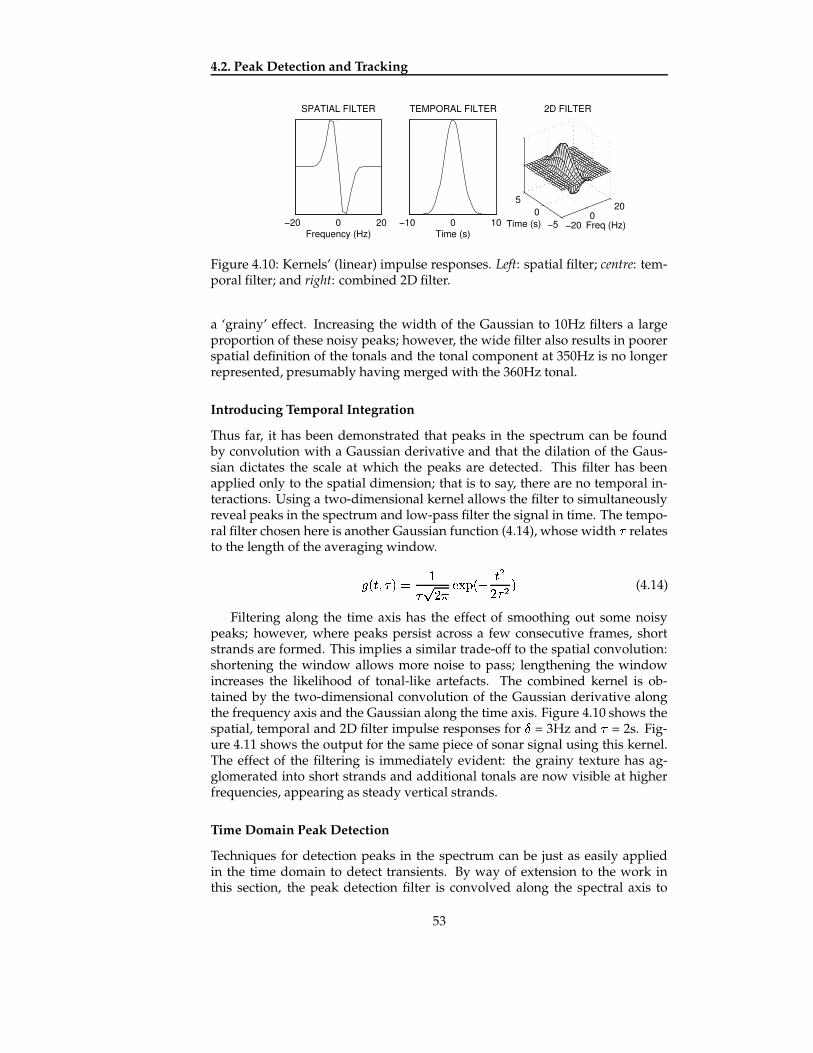
4.2. Peak Detection and Tracking
−20 0 20Frequency (Hz)
SPATIAL FILTER
−10 0 10Time (s)
TEMPORAL FILTER
−200
20
−50
5
Freq (Hz)
2D FILTER
Time (s)
Figure 4.10: Kernels’ (linear) impulse responses. Left: spatial filter; centre: tem-poral filter; and right: combined 2D filter.
a ‘grainy’ effect. Increasing the width of the Gaussian to 10Hz filters a largeproportion of these noisy peaks; however, the wide filter also results in poorerspatial definition of the tonals and the tonal component at 350Hz is no longerrepresented, presumably having merged with the 360Hz tonal.
Introducing Temporal Integration
Thus far, it has been demonstrated that peaks in the spectrum can be foundby convolution with a Gaussian derivative and that the dilation of the Gaus-sian dictates the scale at which the peaks are detected. This filter has beenapplied only to the spatial dimension; that is to say, there are no temporal in-teractions. Using a two-dimensional kernel allows the filter to simultaneouslyreveal peaks in the spectrum and low-pass filter the signal in time. The tempo-ral filter chosen here is another Gaussian function (4.14), whose width z relatesto the length of the averaging window.�4���qU�z1�d �z Ê ��� FAH�I%� * � o��z o � (4.14)
Filtering along the time axis has the effect of smoothing out some noisypeaks; however, where peaks persist across a few consecutive frames, shortstrands are formed. This implies a similar trade-off to the spatial convolution:shortening the window allows more noise to pass; lengthening the windowincreases the likelihood of tonal-like artefacts. The combined kernel is ob-tained by the two-dimensional convolution of the Gaussian derivative alongthe frequency axis and the Gaussian along the time axis. Figure 4.10 shows thespatial, temporal and 2D filter impulse responses for Ç = 3Hz and z = 2s. Fig-ure 4.11 shows the output for the same piece of sonar signal using this kernel.The effect of the filtering is immediately evident: the grainy texture has ag-glomerated into short strands and additional tonals are now visible at higherfrequencies, appearing as steady vertical strands.
Time Domain Peak Detection
Techniques for detection peaks in the spectrum can be just as easily appliedin the time domain to detect transients. By way of extension to the work inthis section, the peak detection filter is convolved along the spectral axis to
53

Chapter 4. Feature Extraction
Frequency (Hz)
Tim
e (s
)
Spectral Gaussian width = 3Hz; Temporal Gaussian width = 2s
0 100 200 300 400 500 600 700 800 900 1000
0
20
40
60
Figure 4.11: Peaks found using Ç = 3Hz and z = 2s.
Frequency (Hz)
Tim
e (s
)
Tonal filter = [10Hz, 1s]; Transient filter = [3s, 3Hz]
0 100 200 300 400 500 600 700 800 900 1000
0
20
40
60
Figure 4.12: Detection of spectral peaks (blue) and impulsive events (red).
find tonals and then separately along the time axis to find transients. The samealgorithm can perform both tasks; in the transient case, the time-frequency ma-trix is simply transposed. Figure 4.12 plots the result of both filters on the sameaxes: the blue, vertical lines are tonals; the red, horizontal lines are transients.The 2D filter for tonal detection had widths of 10Hz and 1s for frequency andtime, respectively; the 2D filter for transient detection had widths of 3s and 3Hzfor time and frequency, respectively. It is worth mentioning that the rhythmo-gram [26] uses convolution with the derivative of a Gaussian to extract therhythm from a time domain signal. The procedure differs in that peaks aredetected in a short-time, windowed estimate of the root-mean-squared energytaken over the entire signal, and the analysis is undertaken at a number ofscales (i.e. Gaussians of various widths are employed).
4.2.3 Peak Tracking
Having presented methods for isolating peaks within a spectrum, a mechanismis required for tracking the peaks through time. This mechanism serves twopurposes. The first of these is to aid noise removal by checking whether a peakpersists throughout sufficient number of frames; if it does not, it is rejected.Peaks which exhibit no continuity in time and frequency (i.e. speckles) areprobably the result of noise. The second purpose is to convert time-varyingpeaks into objects. Processing a signal into a collection of objects imposes astructure upon the signal that provides the starting point for a host of powerfulanalysis techniques, which form the basis of several CASA architectures.
A simple continuity constraint criterion removes a peaks if there are noother peaks within a certain time-frequency context, which is the surroundingregion in time and frequency, parameterised by Ô � and Ô $ . [4] It should benoted that this approach does not track tonals, it simply enforces a rule that all
54

4.3. Modulation Spectrum
Figure 4.13: Tracking peaks in the time-frequency plane. In keeping with theother plots in this section, time runs down the y-axis and frequency is on thex-axis.
peaks should have the potential to form part of a track. The concept of a time-frequency context is analogous to the auditory grouping principle of proximity(see section 1.4). The left plot of Figure 4.13 illustrates a continuity constraint:peaks are retained if there is another peak within the time-frequency context;the empty circle indicates a peak that will be deleted.
Cooke’s CASA model [6] adopts a trajectory-based method for peak track-ing, which uses the derivative of a strand—a collection of peaks already joinedtogether—to inform the search for the peak in the next frame. If a new peakcannot be found, the strand is terminated. The right plot of Figure 4.13 showshow the trajectory approach uses the recent derivative of a strand to search thetime frame.
4.3 Modulation Spectrum
The modulation spectrum is an expression of a signal purely in terms of itsmodulation components. Such a expression is a candidate for a high-level au-ditory representation, following the discovery of cells in the auditory nervethat exhibit fine-tuning to particular modulated stimuli. The application of themodulation spectrum may also arise in a sonar context: the rotation of a ves-sel’s propeller and blades results in a low-frequency modulation in the signalenvelope. Conventional DEMON analysis presently exploits this amplitudemodulation to determine the blade-rate and shaft configuration of a vessel,although such an analysis operates on the envelope of the entire (low-pass fil-tered) signal. The modulation spectrum, by constrast, identifies amplitude andtemporal modulation within narrow bands. Features extracted from this repre-sentation may be useful for classification; alternatively, if envelope modulationinterferes with other algorithms presented in this document, the signal can beresynthesised from the modulation spectrum with these effects removed.
The particular modulation spectrum under discussion here is that of Singhet al. [23] which decomposes the energy in a signal along two dimensions:temporal modulation and spectral modulation. Each point in this two-dimensionalspace corresponds to a ripple component and the signal itself is the weighted sumof all the ripple components. Temporal modulation is variation in the envelope
55

Chapter 4. Feature Extraction
Figure 4.14: Ripple components and the modulation spectrum. The outer plotsshow the ripple components’ envelopes in the time-frequency plane; a cross-section of each indicates the direction of modulation. Each of these is associ-ated with a location in the modulation spectrum—the central plot. Adaptedfrom [23].
in the time-frequency plane along the time axis and is associated with verti-cal ripple components—amplitude-modulated noise is temporal modulationin all channels. Spectral modulation is variation in the envelope in the time-frequency plane along the frequency axis and is associated with horizontal rip-ple components—a harmonic complex is therefore a spectral modulation com-ponent. (Spectral modulation should not be confused with frequency mod-ulation: the former refers to energy varying with frequency; the latter refersto frequency varying with time.) Diagonal ripple components correspond toupsweeps and downsweeps, in which energy varies with both time and fre-quency. Figure 4.14 shows some ripple components and their mapping to themodulation spectrum.
The modulation spectrum is a complex plane; for a complete descriptionof a general signal, the phase of the ripple components must be known in ad-dition to the magnitude. However, for visual comprehensibility, the modula-tion spectrum displays only the magnitude or log magnitude. The modulationspectrum can be divided into four quadrants, i.e. the positive and negativehalves of the temporal and spectral axes, but the lower two are a reflectionof the upper, so only the top half needs to be plotted. The units of temporalmodulation are Hertz and the units of spectral modulation are 1/Hz, 1/kHzor 1/octave.
4.3.1 Computing the Modulation Spectrum
The modulation spectrum is computed in three stages. The first stage is a bankof bandpass filters of equal width, evenly distributed along the frequency axis.A suitable configuration would be the gammatone filterbank described in sec-tion 3.2.4. Next, the envelope of each filter output is obtained and the cross-correlation function (CCF) is calculated for the envelope in every pair of chan-
56

4.4. Phase Modulation
nels (including each channel with itself—the autocorrelation), culminating in� o CCFs for � channels. The second stage collapses the CCFs into a singleauto-correlation matrix, the rows of which are formed from the average of theCCFs for channels of equal frequency separation. For example, the first row isthe average of the CCFs for channels with no separation (i.e. the autocorrela-tions), the second row is the average of the CCFs for one channel separationand so forth. The autocorrelation matrix encodes temporal modulation us-ing the cross-correlation: the increasing lag causes an envelope with periodicAM to repeatedly align with itself resulting in a vertical grating effect. Spec-tral modulation is encoded similarly. For a harmonic complex with no AM, thechannels with a frequency difference equal to multiples of the fundamental fre-quency will align for all lags because the harmonics have a constant, non-zeroenvelope. This produces a horizontal grating effect. The third and final stageis a two-dimensional Fourier transform of the autocorrelation matrix, which isfirst multiplied by two-dimensional tapered window to align its edges. The2D-FFT summarises the grating effect over different directions and frequenciesand hence confines modulations to separate regions of the modulation spec-trum.
4.3.2 Suitability for Sonar
The modulation spectrum described above does not appear to be an appropri-ate representation for a sonar signal. First, the procedure is a computationallyexpensive one; a modest number of channels involves the calculation of a largenumber of cross-correlation functions, e.g. 50 filters requires 1275 CCFs. Sec-ond, modulation spectrum is better suited to natural sounds such as speech,birdsong or other vocalisations, which consist of smooth transitions of har-monic complexes over a reasonable frequency range. The vessel recordingsprovided by QinetiQ contain tonals which are almost static in frequency andamplitude-modulated only at very low frequencies. This low-frequency AMcan be detected economically by applying a short-time Fourier transform tothe envelope of each filter output.
4.4 Phase Modulation
It is routine for a sonar operator to view the tonals present within a vesselacoustic signature via the output of a narrowband display and make a judge-ment as to their origin. At a glance, it is not always evident how these tonalsought to be grouped: they are not guaranteed to be related harmonically andmay only exhibit minute frequency modulations. Furthermore, there is the po-tential for interactions between multiple components of the same frequency.For instance, a signal containing a 50Hz and 60Hz harmonic series will havecoincident components at 300Hz, 600Hz etc. whose magnitude and phase iscontributed to by both series.
This section investigates the automatic grouping of tonals according to com-mon changes in phase and outlines the possibility of separating overlappingcomponents. Three causes of related phase variation may be cursorily iden-tified. First, tonals may be phase-modulated according to the sound source
57

Chapter 4. Feature Extraction
itself. For example, an electrical buzz may naturally vary in frequency accord-ing to the generator or battery; similarly, machinery hum may vary with speed.Second, relative motion of a source with respect to the sonar array (includ-ing surface bobbing) gives rise to Doppler effects, which impress a modula-tion upon the signal. Third, characteristics of the signal path—reflections andrefractions—may modify the phase content of a signal in a consistent way, al-lowing tonals to be associated by the signal channel. Work to date has focusedon establishing the presence of correlated phase changes within the availablesonar recordings.
4.4.1 Phase-tracking using the STFT
The short-time Fourier transform has already been introduced in section 3.1as a method of time-frequency analysis, which involves simply taking the FFTrepeatedly for short sections of the signal. The Fourier transform yields a com-plex spectrum, so a conventional spectrogram displays the magnitude or log-power. Here, our primary interest lies in the short-time phase of the spectrum,which is obtained by taking the angle rather than the magnitude.
The task of grouping tonals involves firstly ascertaining which frequencybins of the spectrogram contain tonal components. For this study, tonals havebeen manually identified in the spectrogram, although techniques for trackingpeaks in the time-frequency plane have already been described in section 4.2.2and could be applied as a preceding stage. Once the frequencies of the tonalshave been isolated, there remains the question of the length of the analysiswindow. A time-limited measurement of phase in the time-frequency planeis not as straight-forward as magnitude. This is easily illustrated by consider-ing the effect on a 100Hz sinusoid. A one-second frame will contain 100 peaksand troughs so that the following frame (assuming they are placed end-to-end)will have the same phase. A frame shortened to 0.5s will span 50 periods and a0.25s frame will span 25 periods; in both cases, alignment will still be preservedbetween frames. For a frame length of 0.125s, however, only 12 and a half pe-riods will be captured, so the frame will terminate halfway through a periodand the next frame will effectively begin in anti-phase. In order to counteractthis artefact, either the system must adjust the phase to account for the slidingwindow, or a window length must be chosen which always corresponds to anatural number of periods. As the signal components inspected in the follow-ing sections are all multiples of 50Hz or 60Hz, the latter approach was adoptedand a window length of 0.5s was used.
Assuming for now this careful choice of frame length, it is possible to trackthe phase of each tonal bin and be certain that an unmodulated tonal at thecentre frequency (CF) will show the same phase at each step. If a tonal is ata frequency slightly higher than the bin CF, then an advance in phase will beobserved at each frame; correspondingly, a frequency slightly lower than theCF will cause a lag in phase. A modulated tonal is a combination of these two,as it drops above and below the CF, causing the phase to modulate. These fourscenarios are depicted in Figure 4.15.
Because the phase is measured around a circle, each full period is accom-panied by a jump, so it is necessary to unwrap the phase. Moreover, in orderto make effective comparisons of the phase variations, the unwrapped phasein each bin is normalised by the centre frequency. The rationale for doing
58

4.4. Phase Modulation
Figure 4.15: Schematic illustration phase modulation. Note the phase of eachperiod within the analysis window.
this is best understood in physical terms: if a superposition of waves is com-pressed and expanded—and hence modulated to a certain extent—then theeffect upon the phase of a low-frequency sinusoid (with a long wavelength)will be less marked than the effect upon high-frequency sinusoid (with a shortwavelength). Thus normalisation evens the phase modulation for all frequen-cies.
Figure 4.16 shows the phase of seven harmonic components in a sonar sig-nal. The phase of all the components lags a small amount with each frame,indicating that the fundamental frequency is actually slightly less than 50Hz.A closer examination of the phase tracks also reveals curvature that varies in acorrelated fashion, most noticably, a change in frequency at about 30 seconds.It may be noted that there is a constant phase difference between the tracks;this is not an issue, as the primary concern lies in how the phase varies, i.e., itsderivative.
4.4.2 Measuring Fluctuations
It has been noted that the linear trend in the phase of a component is indicativeof its frequency in relation to the centre frequency of the FFT bin. For this rea-son, the fact that the phase tracks share a linear trend merely emphasises theirharmonicity; it does not indicate whether they fluctuate in a related manner.Removing the linear trend cancels the contribution of the frequency differencewith the channel (and the constant phase term) and retains only how the tonalsvary about their average frequency. The choice of window length in the STFTis less crucial now, as a window that does not a fit an exact number of periodsproduces a linear slope in the phase, which we are now going to remove. Thatsaid, it is best to avoid a situation where a window terminates halfway througha period because the phase jump between frames approaches Õ � , which can-not be reliably unwrapped. Measure to counteract this problem are discussedin section 4.4.4
The removal of the linear component in each track can be achieved by ex-
59

Chapter 4. Feature Extraction
Frequency (Hz)
Tim
e (s
)SPECTROGRAM
0 100 200 300 400 500
20406080
100
0 50 100−0.6
−0.4
−0.2
0
0.2
Time (s)
Pha
se, r
ads
wrt.
1H
z 50Hz100Hz150Hz200Hz250Hz300Hz350Hz
0 50 100−0.04
−0.02
0
0.02
0.04
Time (s)
Det
rend
ed P
hase
50Hz100Hz150Hz200Hz250Hz300Hz350Hz
Figure 4.16: Modulation of tonal components for a 100-second sonar record-ing. The upper panel is a spectrogram revealing a 50Hz harmonic series; themiddle panel plots the phase of each component as it changes with time (nor-malised wrt. 1Hz); the lower panel plots the same phase, with the linear trendsubtracted.
60

4.4. Phase Modulation
plicitly finding the trend and then performing a subtraction. Alternatively, thederivative of the phase track can be found and then the mean subtracted (themean derivative being the average slope); re-integrating then reproduces theoriginal track with the trend removed. The latter technique suits an adaptivevariant of the algorithm, as a local mean can be subtracted3 from the deriva-tive, although this may result in slow-changing features being ‘smoothed out’.The result of removing the linear trend from the phase tracks is shown thelower panel of Figure 4.16. The tracks corresponding to 50Hz, 150Hz, 250Hzand 350Hz fluctuate almost precisely in unison; 100Hz appears to trace thesame shape and may be simply affected by noise; 200Hz and 300Hz show nocorrelation4.
4.4.3 The Effect of Noise
Upon examining the STFT phase derivative of a number of tonals, as in theprevious section, it is clear that some tracks are related and that some tracks arenot. However, for some tonals, such as the phase track corresponding to 100Hzin the lower panel of Figure 4.16, it is unclear whether the track is following anindependent course, or actually belongs with the others and has simply beendisplaced by noise. In order to answer this question, a means of determiningthe impact of noise upon the phase is required.
Any given observation of phase O�Ö1����� , whether it is from a spectrogrampixel or the Hilbert transform, we shall assume has arisen from the interactionof two complex components: the signal with phase O4×N����� , and some noise withphase O C ����� . Magnitudes for the observation, signal and noise are also knownto be g Ö ����� , g ×N����� and g C ����� , respectively, allowing the sum of the componentsto be expressed as (4.15).g Ö8������{ |ÙØ#Ú�Û�Ü�Ý g × ����� { |ÙØ#ÞqÛ�Ü�Ý � g C ����� { | ØNß�Û�Ü�Ý (4.15)
The question that this section intends to answer is: if the probability distribu-tion for the noise and the signal-to-noise ratio (i.e. the ratio of magnitudes g ×and g C ) are both known, what is the mean departure in phase àd¼ � O�Öá*rO × � ½ ?
From this point on, complex values will be expressed by their real andimaginary parts, as opposed to polar form. For our purposes, the real andimaginary parts of the noise are governed independently by identical Gaus-sian distributions whose variance is unity. The mean magnitude of a complexnumber drawn from this distribution can be obtained by multiplying the mag-nitude function with the probability distribution and integrating over the com-plex plane
àa¼ � ÈR � ½ ���� xdx yD y � Q o � ¡ o FAH�Iãâ4* ��Q o � ¡ o �� ä �?QG� ¡ � ���'� (4.16)
where ÈR is the complex noise signal and Q and ¡ index the real and imaginaryaxes, respectively. This integration can be performed by observing that the
3This is equivalent to a low-pass filter.4In the absence of any ground truth for these signals, the accuracy of these results cannot be
wholly confirmed. However, a recent presentation at the QinetiQ Winfrith site contained plotsshowing similar phase tracks. The procedure can also be tested on artificial signals.
61

Chapter 4. Feature Extraction
−10 −5 0 5 100
0.5
1
1.5
SNR, dB
Exp
ecte
d ph
ase
erro
r, ra
dian
s
Figure 4.17: Mean change in phase for different SNRs. At lower SNRs (noisy)the expected change in phase approaches å o . At higher SNRs (clean) the ex-pected change in phase approaches zero.
distribution is radially symmetric about the origin and so integrate a single‘slice’ of the Gaussian over 3 9<Uq�Ææ:5 along the real axis and rotate the planefigure around the origin to form a volume by multiplying5 by ��� .
A similar expression can be formulated to find the average absolute angleof the noise component, which is å o if the angles returned by ç�è -qé ç � are in therange [ *W� , �i� ].
àd¼ �Ùê ÈR � ½ ���� xax yD y vvv ç'è -0é ç � ¡Q vvv FAH2Iëâ4* ��Q o � ¡ o �� ä �'Q�� ¡ � � (4.17)
Now we are in a position to say how far, on average, the phase of the noise sig-nal will deviate from zero radians. It is a small step then, to introduce a signalcomponent as a real value6 and re-evaluate the integral. Note that because theaverage magnitude of the noise is
� ����� , the signal magnitude must be scaledby this value. So, for a signal-to-noise ratio ì , given in decibels, the expecteddeparture from phase àa¼ � O Ö *:O�×�� ½ , in radians, is given by (4.19).b Å � �����í²��§9'î8ï E M (4.18)
àa¼ � O Ö *rO�×�� ½ ��#� xax@yD y vvvv ç�è -qé ç �ëâ ¡QÂ� b ä vvvv F0H�Iãâ4* ��Q o � ¡ o �� ä �?QG� ¡ (4.19)
By numerically evaluating (4.19), the expected error in phase has been ob-tained for a variety of SNRs and plotted in Figure 4.17. This working has as-sumed that the noise has a Gaussian distribution, but the same approach canbe used for other distributions, by appropriately altering the integral.
4.4.4 Non-linear Filtering
Up to this point we have only considered the effect of broad spectrum noiseon the phase track; another problem which has been persistently encountered
5The area centroid of the spectral slice is one.6The reference signal could have any phase, as the probability distribution for phase for a noise
signal is uniform. A purely real (or imaginary) component is simpler to work into the equation.
62

4.4. Phase Modulation
0 100 200−5
0
5A. Clean phase
Time (s)
radi
ans
0 100 200−50
0
50B. Unwrapped phase
Time (s)
radi
ans
0 100 200−2
0
2C. Detrended phase
Time (s)
radi
ans
0 100 200−5
0
5D. Noisy phase
Time (s)ra
dian
s0 100 200
−20
0
20E. Unwrapped phase
Time (s)
radi
ans
0 100 200−5
0
5F. Detrended phase
Time (s)
radi
ans
Figure 4.18: Illustration of how phase artefacts appear. A: clean, wrappedphase track; B: clean, unwrapped phase track; C: clean, detrended phase track;D: wrapped phase track with glitch at 50s; E: noisy unwrapped phase track; F:noisy detrended phase track.
when examining the phase tracks are glitches. Owing to the cumulative effectof unwrapping the phase and the estimation and removal of a linear trend, anerror in just one measurement of the phase can misalign an entire track. Thissort of occurrence is illustrated in Figure 4.18. Panel A plots the phase of asinusoid with a small amount of noise. The unwrapped phase is a noisy linearfunction (B); subtracting the linear trend gives a zero-mean noise residual (C).The problem arises when glitches at a few isolated points cause the phase tojump to the opposite side of the unit circle so that the unwrapped phase nolonger follows a smooth trend. In the figure, this scenario is depicted in thebottom three plots (D–F)—the jump occurs at 50 seconds.
Figure 4.19(A) shows the same problem for two tracks obtained from asonar recording over 100 seconds. The two tracks correspond to tonals at360Hz and 420Hz and form part of the same harmonic complex. It is evidentthat the fluctuations in phase about the linear trend would be the same for bothtonals, were it not for the discontinuities at 48s and 87s in the 360Hz and 420Hztracks, respectively. (To visualise the effect of removing the glitches, imag-ine the sharp, vertical jumps ‘shrinking’ so that the ends are joined together.)Clearly, if an algorithm is going to compare tonals for common fluctuations inphase, then a filter is required to eliminate these artefacts prior to making thecomparison.
Phase jumps can be removed by modifying the derivative of the unwrappedphase, in which discontinuities appear as sharp upward or downward spikes.For example, the unwrapped phase in Figure 4.18(E) has a constant derivativeat all times except the glitch, where the derivative is a negative spike. Hence, toremove the discontinuities implies taking the derivative, deleting positive andnegative spikes with a large magnitude, and reintegrating. The filter used toremove the spikes has to be chosen carefully. An averaging filter (e.g. a Gaus-sian or mean kernel) is unsuitable, as spikes are smoothed into the surroundingregion, which we want as far as possible to remain unaffected.
A more appropriate strategy for removing spikes would be a median filter,which replaces each value in the derivative with the median of the surroundingpoints. Like the mean filter, this procedure is also characterised by a smooth-
63

Chapter 4. Feature Extraction
0 20 40 60 80 100 120 140 160 180 200−0.02
−0.01
0
0.01
Time (s)
Rad
ians
wrt.
1H
zB. DETRENDED PHASE − MEDIAN FILTER
360Hz420Hz
0 20 40 60 80 100 120 140 160 180 200−0.02
−0.01
0
0.01
Time (s)R
adia
ns w
rt. 1
Hz
A. DETRENDED PHASE − NO FILTER
0 10 20 30 40 50 60 70 80 90 100−0.01
−0.005
0
0.005
0.01
Time (s)
Rad
ians
wrt.
1H
z
C. DETRENDED PHASE − THRESHOLD/SPLIT−WINDOW FILTER
360Hz420Hz
360Hz420Hz
Figure 4.19: Artefacts in a sonar phase track. Top: unmodified phase track;middle: phase track with a median-filtered derivative; bottom: phase track witha threshold-filtered derivative.
ing effect, with the added difference that large or small outlying values (i.e.spikes) do not bias the median. The result of median smoothing the derivativeis shown in Figure 4.19(B); a window corresponding to 5 seconds (2.5 secondseither side) was used. Although the process has removed the sharp jumps, ithas also detrimentally altered the shape of the phase track; similar results areobtained for shorter and longer window sizes. The poor performance of themedian filter stems from its application to the derivative. Tiny differences in theslope accumulate over time to create a broad trends; the application of a me-dian filter upsets these differences to such an extent that the output no longerresembles the input.
The requirement that the phase-derivative remain unaffected to the greatestpossible degree, motivated the search for another non-linear filter. A particu-larly successful filter was formulated, which uses a hard threshold to detectdiscontinuities. Positive and negative spikes in the derivative are flagged forremoval if they exceed the global variance by some factor ð . Once detected,each spike is replaced with an estimate formed by averaging the values in asplit window a short distance either side. The threshold is chosen to captureonly the severest spikes, in order to minimise the effect upon other regions ofthe derivative. A threshold of ð ñ�§9 was used to produce the phase tracks inFigure 4.19(C), which show substantially better agreement.
64

Chapter 5
Conclusions and Future Work
The incorporation of auditory models into sonar algorithms is still very muchan open area for research. To date, most auditory-motivated sonar modelshave concentrated on the processing of transient events, which is perhaps un-surprising in view of the following: i) owing to their energy, sharp onset andbrief duration, transient events are perceptually outstanding; ii) the interrup-tion from transients has an adverse effect upon tonal-based classifiers, fuellingresearch as to how to minimise their impact; iii) transient datasets are morereadily available; and iv) while much effort has been poured into minimisingtonal emissions, occasional ‘clanks’, ‘knocks’ and ‘pops’ are unavoidable, sothat accurate transient classification is a tactical advantage.
Aspects of a vessel acoustic signature which have received less attentionfrom the auditory modelling community are tonals, amplitude modulation andrhythm1 (although rhythm has been used by Tucker to provide a context fortransient events [27]). However, it is primarily the frequencies and amplitudesof tonal components which provide the most reliable features for a classifier.The precise measurement of a tonal set is impeded by the presence of broad-band noise, transient noise and other tonals, which cause indiscernibility, in-termittence and interference. Spectral structures familiar to a human listener(e.g. a vowel sound) are often obscured by everyday sounds of comparablequality, for instance, running water, a door slamming and musical notes, re-spectively. Despite this, our ability to listen is not compromised until the noiseconditions are quite severe. The analysis of frequency structure is central toall the non-sonar CASA models reviewed in this report and similar techniquesmay be employed in the task of detecting and organising tonal componentswithin a sonar signal. The remainder of this chapter outlines areas for futureresearch, which span the problems of tonal detection, tracking and groupingfrom an auditory perspective.
5.1 Future Work
This section presents four questions that are prompted by the discussion inthis document. The first two questions relate to the low-level function of the
1There is some degree of overlap between AM and rhythm: low-frequency AM may be per-ceived as a fast rhythm.
65

Chapter 5. Conclusions and Future Work
ear and its relevance to sonar: temporal processing and lateral inhibition. Thelast two questions are motivated by hearing, specifically, the perceptual effectsassociated with amplitude modulation and a possible role for computationalauditory scene analysis in the separation of sonar sounds.
Does temporal processing offer any advantages over a traditional spectralanalysis when applied to narrowband sonar algorithms?
Narrowband sonar analysis uses methods based on the Fourier transform suchas a spectrogram to assess the tonal structure within a vessel acoustic signature.Tonal detection (by a human viewer or a machine) proceeds according to howmuch energy is present in the spectrum at certain frequencies—a spectral anal-ysis. Inevitably, noise sources contribute energy to the spectrum in an unevenfashion, leading to the indiscernibility of tonal spikes. In other words, with theaddition of noise, it becomes increasingly difficult to say whether the energy ina discrete frequency bin should be ascribed to a tonal or to noise.
Studies of human audition have revealed that the signal transforms of theear incorporate a spectral analysis that is accomplished by measuring the ex-tent to which the basilar membrane vibrates along its length (place encoding).However, the temporal fine structure of the vibration at a single place, as trans-duced by the inner hair cells, also serves to enhance the frequency content ofa signal by temporal encoding. It is this secondary stage of temporal process-ing, which sonar systems presently lack. Accordingly, a study is required toexamine how a sonar algorithm benefits from a temporal analysis of the sig-nal. In particular, temporal processing might: i) allow for greater precisionin the measurement of frequency components; ii) improve robustness againstnoise; iii) provide a smooth encoding of frequency transitions; and iv) providea means of associating components in remote frequency regions by features oftheir fine structure.
Is lateral inhibition preferable to spectral normalisation?
Narrowband analysis is usually followed by a spectral normalisation stage,which subtracts from each bin an estimate of the local noise energy, obtainedby averaging the energy under a split window centered on the bin. (A splitwindow is used to prevent a tonal resolved across one or more bins from sub-tracting energy from itself.) This procedure highlights regions of contrast andso assists the sonar operator in visually distinguishing tonal features within aspectrogram. Assuming the same split window is used for all bins, spectralnormalisation can be interpreted and implemented as a high-pass spatial filter.
Lateral inhibition is behaviour observed in collections of nerve cells, whichachieves a similar effect to spectral normalisation: the response of a cell is re-duced by the activity of neighbouring cells. Lateral inhibition is active in boththe eyes and ears, implying that the sharp features of visual and auditory sen-sations are enhanced prior to any processing by the brain. The similarity be-tween spectral normalisation and lateral inhibition prompts an investigationinto the advantages of one method over the other when used in a sonar appli-cation.
One problem inherent in spectral normalisation is the mutual inhibition oftwo tonals, that is, the possibility that one tonal (or both) will be interpreted as
66

5.1. Future Work
Figure 5.1: Co-modulation masking release. A: the bandwidth of the modu-lated noise is confined to a single auditory filter so the tonal in undetectable;B: the bandwidth of the modulated noise extends over a number of auditoryfilters so the tonal is detectable.
noise by the other and subtracted, resulting in an energy loss. It must be estab-lished whether lateral inhibition suffers the same drawback, and if not, hownormalisation schemes may be improved as a result. Finally, several workerscited by Shamma [22] have noted that introducing instability into the recurrentLIN (see Chapter 4) in conjunction with a non-linear activation function at theoutput units, brings about a number of short-term memory effects (hysteresis).Further work in lateral inhibition should explore the possibility of exploitingthese within a sonar context, with a view to aiding tonal completion.
Can the amplitude modulation of vessel noise aid the detection of tonals?
DEMON analysis is concerned with extracting useful information from the am-plitude modulation impressed upon on the envelope of a broadband noise sig-nal. Specifically, when a harmonic series is present in the frequency spectrumof the envelope, the fundamental corresponds to the blade rate and the ampli-tudes of the harmonics relate to the number and configuration of the blades.Hence the noise component of a vessel signature, whilst a nuisance for tonal-based classification, can be considered an important source of features in itself.However, if tonals are the key concern, accounting for the modulated characterof the noise signal will be helpful in cancelling it.
Remarkably, the human auditory system is able to cancel a broadband,amplitude-modulated noise signal and expose tonals, which would otherwisebe masked by unmodulated noise. This can be demonstrated by centering anarrow band of amplitude-modulated noise on a tonal and increasing its band-width. When the noise falls entirely under the same auditory filter as the tonal,the threshold for tonal detection is high. As the bandwidth of the noise is in-creased, other auditory filters capture the modulation and the threshold fordetection is lowered. This phenomenon is referred to as co-modulation maskingrelease (CMR) [10], as the coherent modulation of a noise signal across a suf-ficiently wide block of auditory filters ‘releases’ a stimulus from masking (seeFigure 5.1). Evidently, CMR is of direct relevance to sonar processing, owingto its ability to unearth tonals immersed in modulated noise. Consequently, aportion of the remaining time will be dedicated to applying models of CMR tosonar signals.
67

Chapter 5. Conclusions and Future Work
How might a sonar system be said to listen? Is it possible to segegrate under-water sounds to improve the performance of a human or machine classifier?
The final research area outlined in this report is inspired by conventional CASAmodelling and considers the application of high-level organisational principlesto group auditory objects into streams. Such an advance would give rise to ahost of useful technologies, which were outlined in the opening chapter of thisdocument: the segregration of concurrent underwater sources prior to classifi-cation would no doubt lead to an increase in a classifier’s performance; alter-natively, the colour-coding of features on a narrowband display according to acommon source would allow a sonar operator to deal in objects not raw data.
The data-driven CASA architecture envisaged for this type of applicationwould generally isolate features in the time-frequency plane which exhibit con-tinuity (e.g. static and moving frequency components and transients) and thengroup them according to commonalities in amplitude and frequency. The for-mulation of a CASA model for a sonar task, particularly one that performstonal grouping, will necessarily differ from the CASA models that have gonebefore. The tonals in a vessel signature are not overtly modulated as those ofspeech and music signals are, so in order to group them together, an algorithmmay have to partially resort to sub-audible regularities, such as changes in thephase of frequency components. Nevertheless, there remain numerous audiblecues that may be incorporated without compromise: common onset and offset,harmonicity, common pitch variation and common AM are some examples.
68

Bibliography
[1] B. Boashash and P. O’Shea. A methodology for detection and classificationof some underwater acoustic signals using time-frequency analysis tech-niques. IEEE Trans. on Acoustics, Speech, and Signal Processing, 38(11):1829–1841, 1990.
[2] A.S. Bregman. Auditory Scene Analysis: The Perceptual Organisation ofSound. The MIT Press, London, 1990.
[3] G.J. Brown. Computational Auditory Scene Analysis: A Representational Ap-proach. PhD thesis, University of Sheffield, September 1992.
[4] G.J. Brown and S.N. Wrigley. Feasibility study into the application of com-putational auditory scene analysis techniques to sonar signals. Techni-cal report, University of Sheffield, Department of Computer Science, May2000.
[5] W.S. Burdic. Underwater Acoustic System Analysis. Prentice-Hall, Inc., En-glewood Cliffs, NJ 07632, 1984.
[6] M.P. Cooke. Modelling Auditory Processing and Organisation. PhD thesis,University of Sheffield, May 1991.
[7] E. de Boer and H.R. de Jongh. On cochlear encoding: potentialitiesand limitations of the reverse-correlation technique. J. Acoust. Soc. Am.,63(1):115–135, 1978.
[8] D.P.W. Ellis. Prediction-driven computational auditory scene analysis. PhDthesis, Massachusetts Institute of Technology, June 1996.
[9] O. Ghitza. Temporal non-place information in the auditory-nerve firingpatterns as a front-end for speech recognition in a noisy environment. J.Phonetics, 16:109–123, 1988.
[10] M.P. Haggard, J.W. Hall, and J.H. Grose. Comodulation masking re-lease as a function of bandwidth and test frequency. J. Acoust. Soc. Am.,88(1):113–118, 1990.
[11] I.P. Kirsteins, S.K. Mehta, and J. Fay. Separation and fusion of overlappingunderwater sound streams. In Proceedings of EUSIPCO 2000, volume 2,pages 1109–1113, 2000.
69

BIBLIOGRAPHY
[12] V.R. Lesser, S.H. Nawab, and F.I. Klassner. IPUS: an architecture for theintegrated processing and understanding of signals. Artificial Intelligence,77:129–171, 1995.
[13] R.J. McAulay and T.F. Quatieri. Speech analysis/synthesis based on asinusoidal representation. IEEE Trans. on Acoustics, Speech, and Signal Pro-cessing, ASSP-34(4):744–754, 1986.
[14] R. Meddis. Simulation of auditory-neural transduction: Further studies.J. Acoust. Soc. Am., 83(3):1056–1063, 1988.
[15] D.K. Mellinger. Event Formation and Separation in Musical Sound. PhDthesis, Stanford University, December 1991.
[16] B.C.J. Moore. An Introduction to the Psychology of Hearing. Academic Press,London, fifth edition, 2003.
[17] J.O. Pickles. An Introduction to the Physiology of Hearing. Academic Press,London, second edition, 1988.
[18] F. Pineda, K. Ryals, D. Steigerwald, and P.M. Furth. Acoustic transientprocessing using the hopkins electronic ear. In Proceedings of WCNN 95,volume 1, pages 136–141, July 1995.
[19] K.J. Powell, T. Sapatinas, T.C. Bailey, and W.J. Krzanowski. Applicationof wavelets to the pre-processing of underwater sounds. Statistics andComputing, 5:265–273, 1995.
[20] M.D. Riley. Speech Time-Frequency Representations. Kluwer Academic Pub-lishers, 1989.
[21] S. Seneff. A joint synchrony/mean-rate model of auditory speech process-ing. J. Phonetics, 16:55–76, 1988.
[22] S.A. Shamma. Speech processing in the auditory system II: Lateral inhibi-tion and the central processing of speech evoked activity in the auditorynerve. J. Acoust. Soc. Am., 78(5):1622–1632, 1985.
[23] N.C. Singh and F.E. Theunissen. Modulation spectra of natural soundsand ethological theories of auditory processing. J. Acoust. Soc. Am.,114(6):3394–3411, 2003.
[24] Q. Summerfield and P.F. Assmann. Perception of concurrent vowels: Ef-fects of harmonic misalignment and pitch-period asynchrony. J. Acoust.Soc. Am., 89(3):1364–1377, 1991.
[25] A. Teolis and S. Shamma. Classification of transient signals via auditoryrepresentations. Technical Report TR 91-99, University of Maryland, Sys-tems Research Center, 1991.
[26] N.P. McAngus Todd and G.J. Brown. Visualization of rhythm, time andmetre. Artificial Intelligence Review, 10:253–273, 1996.
[27] S.A. Tucker. An ecological approach to the classification of transient underwa-ter acoustic events: Perceptual experiments and auditory models. PhD thesis,University of Sheffield, November 2003.
70

BIBLIOGRAPHY
[28] M. Unoki and M. Akagi. A method of signal extraction from noisy signalbased on auditory scene analysis. Speech Communication, 27:261–279, 1999.
[29] T. Verma and T. Meng. Sinusoidal modeling using frame-based perceptu-ally weighted matching pursuits. In Proc. Int. Conf. Acoustics, Speech andSignal Processing (ICASSP) 1999, 1999.
[30] A.D. Waite. Sonar for Practising Engineers. Thomson Marconi Sonar Lim-ited, Dolphin House, Ashurst Drive, Bird Hall Lane, Cheadle Heath,Stockport, Cheshire SK3 0XB, 1998.
71