auditory processing - unimi.ithomes.di.unimi.it/avanzini/downloads/asmc_handouts/asmc_ch5.pdf ·...
TRANSCRIPT
Chapter 5
Auditory processing
Federico Avanzini
Copyright c⃝ 2005-2019 Federico Avanziniexcept for paragraphs labeled as adapted from <reference>
This book is licensed under the CreativeCommons Attribution-NonCommercial-ShareAlike 3.0 license. Toview a copy of this license, visit http://creativecommons.org/licenses/by-nc-sa/3.0/, or send a letter to
Creative Commons, 171 2nd Street, Suite 300, San Francisco, California, 94105, USA.
5.1 Introduction
If a tree falls in a forest and no one is around to hear it, does it make a sound? The origin of this riddleis unclear, but it is often referenced whenever one wants to address the topic of the division betweenperception of an object and how an object really is. If the tree exists regardless of perception, then it willproduce sound waves when it falls. However, no one knows how these sound waves will actually soundlike. Sound as a mechanical and fluid-dynamical phenomenon will occur, but sound as a sensation willnot occur.
So what is the difference between what something is, and how it appears? Subjective idealismanswers to this question by saying that “to be is to be perceived”. As far as sound in particular isconcerned, some contemporary metaphysicians propose proximal theories of sound. According to thesetheories, sounds are sensations or qualitative aspects of auditory perception, they are conceived of asinternal events, as mental episodes, or proximal stimulations. This view emphasizes the high correlationbetween felt properties of sounds and properties of perceptual system. As opposed to proximal theories,distal theories consider the nature of sounds to be found in distal properties, processes or events in themedium inside (or at the surface of) sounding physical objects. Medial theories regard sounds as beinglocated between the sounding objects and the hearer: sounds are sound waves.
5-2 Algorithms for Sound and Music Computing [v.February 2, 2019]
���������������������������������������������������������������
���������������������������������������������������������������
��������������
������
������������
������������������������������������������������������������������������
������������������������������������������������������������������������
���������������
���������������
������������
������������
ear canal
pinna
concha
malleusincus
stapes
round windowoval window
cochlea
auditory nerve
eustachian tube
external middle inner
bone
bone
membranetympanic
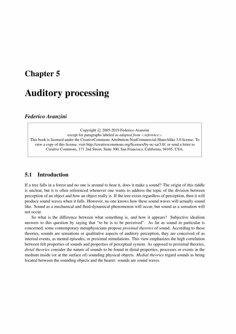
Figure 5.1: Schematic, not-in-scale, drawing of the human peripheral auditory system.
5.2 Anatomy and physiology of peripheral hearing
Figure 5.1 provides a representation of the anatomy of the human peripheral auditory system. Thiscomprises: the external ear, which has been already examined in Chapter Sound in space and is basicallycomposed by the pinna and the ear canal; the middle ear, which comprises three tiny bones or ossiclesand transforms into mechanic oscillations the acoustic pressure disturbances that arrive on the tympanicmembrane; and the inner ear, where mechanical oscillations are transduced into oscillations of the fluidthat fills the cochlea.
We only address the peripheral auditory system and do not speak of the central system. Higher-levelfunctions not known well.
5.2.1 Sound processing in the middle and inner ear
5.2.1.1 The middle ear
Figure 5.2(a) provides a schematic representation of the mechanics of the middle ear: the eardrum sep-arates the outer ear from the middle ear cavity, in which a chain of three ossicles is found: these arethe malleus (a hammer-shaped bone), the incus (an anvil-shaped bone), and the stapes (a stirrup-shapedbone). This chain of ossicles acts like a lever in response to vibrations of the eardrum; the footplate ofthe stapes is in contact with the inner ear through the oval window at the base of the cochlea and acts likea piston on the fluid inside the cochlea.
Normally, the middle ear cavity containing the ossicles is closed off from its surroundings by theeardrum on one side and the eustachian tube on the other. However, the eustachian tube, which isconnected to the upper throat region, is opened briefly when swallowing. External pressure changes,that can be experienced e.g. during mountain hiking, flying, or diving, can produce changes the restingposition of the eardrum with a consequent shift of the working point in the transfer characteristic of themiddle ear ossicles and a reduction of hearing sensitivity. Normal hearing is resumed by swallowingbecause the opening of the eustachian tube allows to equalize the air pressure in the middle ear with thatof the environment.
The middle ear acts as a mechanical energy transformer. The tympanic membrane operates over awide frequency range as a pressure receiver and is firmly attached to the long arm of the malleus. The
This book is licensed under the CreativeCommons Attribution-NonCommercial-ShareAlike 3.0 license,c⃝2005-2019 by the authors except for paragraphs labeled as adapted from <reference>

Chapter 5. Auditory processing 5-3
oval window
middle ear cavity
stapes
ear canal
eardrum
incus
eustachian tube
malleus
pivot axis
(a)
100 1000 10000−10
0
10
20
30
40
f (Hz)
Ga
in a
t o
va
l w
ind
ow
(d
B)
(b)
Figure 5.2: Middle ear function; (a) scheme of the mechanical action , and (b) qualitative magnituderesponse (note that this plot does not report real measured data, it is an illustrative example in qualitativeagreement with real data).
lever system formed by the three ossicles increases the force transmitted from the tympanic membraneto the stapes by means of two main mechanisms: first, the ossicle system lever provides a lever ratio ofalmost 2 thanks to the different lengths of the arms of the malleus and incus; second, the large surfaceratio between tympanic membrane and oval window (about 35 ) again provides a gain with respect tothe magnitude of the acoustic pressure. The transformation operated by the middle ear can be visualizedby means of its transfer function, from acoustic pressure in the ear canal to fluid pressure in the cochlea.A qualitative magnitude response is shown in Fig. 5.2(b). The forward impedance gain is about 30 dB.Filtering effects due to resonances of the middle ear cavity and mechanical parameters of the ossiclesystem produce a peak in the range 1 − 2 kHz, so that all-in-all the middle ear behaves like a bandpassfilter.
The main role of the middle ear is to provide an impedance matching between air and cochlearfluid: if energy were transmitted directly from acoustic pressure to the cochlea, this would produce anenergy loss of about 30 dB. If we compare this number with Fig. 5.2(b) we can conclude that the humanmiddle ear provides an almost perfect impedance match in the frequency range around 1 kHz. Anotherimportant function of the middle ear is to act as a protection mechanism against very loud sounds: whenthe acoustic pressure exceeds a certain level, an acoustic reflex is generated so that movement of theossicles is inhibited by muscular contraction and the amount of energy transmitted to the inner ear islowered. However, because of relatively high latencies of muscle activations, the acoustic reflex is noteffective for very fast transient sounds (that is why a shot in your ear hurts).
5.2.1.2 The cochlea and the basilar membrane
The inner ear is constituded by the cochlea, which is shaped like a snail (hence its name) and is embeddedin the extremely hard temporal bone (see Fig. 5.1). The cochlea forms 2 and a half turns and has a totallength of about 35 mm. If we “linearize” this snail-like shape we obtain the schematic representationgiven in Fig. 5.3, where all the main elements of the cochlea can be recognized.
The footplate of the stapes is in direct contact with the interior of the cochlea through the membra-neous oval window. At the interior, the cochlea is divided into three channels (or scalae), which areseparated by two membranes. The thicker membrane is the basilar membrane (BM), while the thinner
This book is licensed under the CreativeCommons Attribution-NonCommercial-ShareAlike 3.0 license,c⃝2005-2019 by the authors except for paragraphs labeled as adapted from <reference>

5-4 Algorithms for Sound and Music Computing [v.February 2, 2019]
helicotrema
stapes
oval window
Reissner’s membrane
round window
basilar membrane
bony shelves
base of the cochlea apex of the cochlea
Figure 5.3: Linearized structure of the cochlea.
one is the Reissner’s membrane. Two channels, the scala vestibuli and the scala tympani, run until theapex of the cochlea and are filled with the same fluid, the perilymph. Perilymph has a high sodiumcontent and resembles other extracellular fluids. It is in direct contact with the cerebrospinal fluid ofthe brain cavity. The third channel, the scala media, ends blindly before the apex of the cochlea and isfilled with a different fluid, the endolymph. Endolymph is in contact with the vestibular system and has ahigh potassium content. Loss of the potassium ions from the scala media by diffusion is reduced by thetight membrane junctions of the cells surrounding the scala media. Any losses are rapidly replaced by anion-exchange pump with high energy requirements found in the cell membranes of a specialized groupof cells on the outer wall of the cochlea. This ion exchange generates a positive potential of about 80 mVin the scala media with respect to the perilymph, with the Reissner’s membrane providing chemical iso-lation between the compartments. From a hydromechanical point of view, the scala media and the scalavestibuli can be regarded as one unit, since the Reissner’s membrane that separates them is extremelythin and light, and therefore mechanically very compliant.
Oscillations are transmitted from the stapes to the perilymph, and from the fluid to the BM which isdisplaced in a transverse direction. Since the fluids and the walls of the cochlea (surrounded by bone)are essentially incompressible, the fluid volume displayed at the oval window by the movement of thestapes must be equalized. The equalization occurs at the round window, which is a second membrane thatcloses off the scala tympani at the base of the cochlea. In general the oscillation is transmitted from theperilymph to the endolymph and finally to the round window trhrough the BM. However, for very lowfrequencies the equalization occurs through a direct connection between the scalae tympani and vestibuliat the apex of the cochlea, called the helicotrema.
5.2.1.3 Spectral analysis in the basilar membrane
The total length of the BM is something less than 35 mm. Moreover, it is extremely narrow (about0.05 mm) at the very base of the cochlea, and becomes much wider (about 0.5 mm) and thinner towardsthe apex. Due to this particular shape, the BM behaves as a non-homogeneous transmission line. Onecan hypotesize that low frequencies will produce oscillations of the wider and less stiff portion of theBM at the apex of the cochlea, while high frequencies will produce oscillations of the thinner and stifferportion at the base.
In fact many experimental results have confirmed this hypothesis. The peak displacement of the BM
This book is licensed under the CreativeCommons Attribution-NonCommercial-ShareAlike 3.0 license,c⃝2005-2019 by the authors except for paragraphs labeled as adapted from <reference>

Chapter 5. Auditory processing 5-5
dB
f4kHz
x4
x2dB
f2kHz
dB
f1kHz
dB
f500Hz
x2
dB
f250Hz
x4
basilar mem
brane
oval window
helicotrema
Figure 5.4: Qualitative responses to a 1 kHz sinusoidal stimulus at various sites on the basilar mem-brane.
in response to a sinusoidal stimulus has a small amplitude near the base, grows slowly moving along thecochlea, reaches its maximum at a certain, frequency-dependent location, and then dies out very quicklyin the direction of the apex. The fluid surrounding the BM also keeps at rest beyond the point of maximalBM vibration.
In this way the BM acts as a spectrum analyzer in which different frequencies produce maximumdisplacement at different locations. A sinusoid of say 8 kHz will produce a maximum displacementwithin the first few millimiters of the BM, while a sinusoid of say 200 Hz will produce a maximumdisplacement within the last few millimiters. Through this mechanism of frequency separation, energyfrom different frequencies is transferred to and concentrated at different places along the BM. In otherwords, different regions along the cochlea have different characteristic frequencies (CF), to which theyrespond maximally. This separation by location on the BM is sometimes termed the place principle.
Figure 5.4 provides a qualitative illustration of this mechanism. If a 1 kHz tone burst is presented atthe oval window, the responses at different positions of the BM may be represented as different bandpassfilters with a somehow asymmetrical frequency response, and with centre frequencies related to position.Near the oval window the 1 kHz burst produces a short click due to the broadband transient at the setupof the burst, followed by 1 kHz oscillation with very small amplitude. Further along the cochlea inthe direction of the helicotrema the response becomes larger, and the amplitude reaches its maximumroughly at the median position along the BM. Then the amplitude of vibration produced by the burstbecomes quickly smaller and smaller for places in the cochlea located further towards the helicotrema,which correspond to lower and lower resonance frequencies.
Many experiments have been performed on various mammalian cochleae in order to determine aprecise mapping between CF and longitudinal position on the BM (or “tonotopic” mapping). In thecochleae of several species the tonotopic map follows the law
CF = A(10ax − k), (5.1)
where CF is expressed in kHz, x is the distance from the apex expressed as a proportion of BM length(from 0 to 1), a has the same value (a ∼ 2.1) in many species including humans, k also varies onlyslightly in many species (from 0.8 to 1, typically 0.85), while A varies considerably across species anddetermines the range of CFs (e.g. it has been measured to be a high 0.456 in cat, and only 0.164 in
This book is licensed under the CreativeCommons Attribution-NonCommercial-ShareAlike 3.0 license,c⃝2005-2019 by the authors except for paragraphs labeled as adapted from <reference>
5-6 Algorithms for Sound and Music Computing [v.February 2, 2019]
chinchilla). Equation (5.1) provides a simple linear relation between BM position and the logarithm ofCF, which can be assumed to be valid for the basal 75% of the cochlea (i.e., for x > 0.25), while in theremaining 25% apical region CF octaves become more compressed (in general the behavior of the BMnear the apex is less clearly understood than near the base).
5.2.1.4 Cochlear traveling waves
A second effect depicted in Fig. 5.4 is a time delay between the tone burst at the oval window and theresponse of the BM, which increases with increasing distance. Therefore our simplified description ofthe linear dynamics of the BM has to take into account two main effects: spatial frequency resolution onone hand, and temporal effects (time delays), on the other. High frequencies produce oscillations nearthe oval window and with small delay times, while low frequencies travel far towards the helicotremaand show long delay times.
Position-dependent time delays in BM oscillation have been observed experimentally. Typical delayvalues can be of ∼ 1.5 ms for frequencies around 1.5 kHz, and up to 5 ms near the end of the cochlea.This evidence has led many researchers to the conclusion that a pertubation at the oval window producesa mechanical transverse traveling wave on the BM. This mechanical wave is not to be confused withacoustic pressure waves, which propagate in the cochlear fluids at speeds of about 1550 m/s and traversethe cochlea in a few microseconds.
It has to be noted that the elastic fibers that are tensed across the cochlear duct and form the BM areloosely coupled to each other, so that they can be assumed to vibrate almost independently, like stringsof a musical instrument. Due to this weak longitudinal coupling in the BM, many agree that the energydelivered to the cochlea by the stapes is transported principally via pressure waves in the cochlear fluidsrather than by the BM itself. Fluid pressure interacts with the flexible BM, generating coupled “slow”waves that travel from base to apex: a differential pressure wave that propagates in the cochlear fluidsand a displacement wave that propagates on the BM. In this view, although the BM displacement appearsto travel in a wave from base to apex, the energy is in fact carried longitudinally by the fluid rather thanby the BM.
Nowadays the traveling wave model is regarded to be too simplistic in many respects. In particularthe model disregards possible multiple modes of vibrations, so that sites along the radial direction (of acochlear cross-section) do not all vibrate in phase. Some models and also some experimental observa-tions suggest that multiple modes may be present, and that the presence of a summation of at least twomodes may have a role in the stimulation of the stereocilia of inner hair cells (see below), although clearevidence is still lacking. One second open issue regards the longitudinal coupling of the tissues in theBM. Although such coupling is weak, and typically ignored as we have seen, it could potentially propa-gate a significant amount of energy longitudinally, so that multiple pathways for energy propagation maybe present in the cochlea.
5.2.1.5 The organ of Corti and the haircells
We still have to understand how the mechanical vibrations of the BM are transduced into electrical signalsto be propagated in the auditory nerve. To this end we have to take a closer look at anatomical details ofthe cochlea.
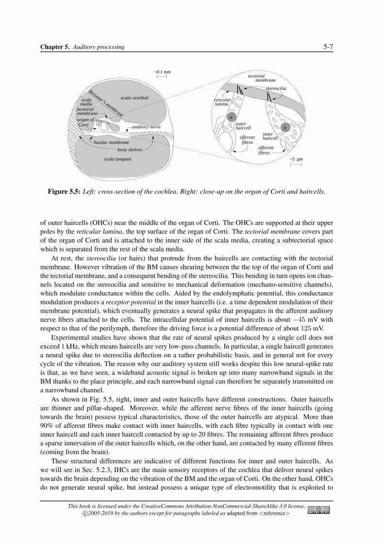
Figure 5.5 (left) depicts a section of the cochlea, and shows that the BM supports the organ of Corti,in the scala media. The function of the organ of Corti is precisely the transformation of mechanicaloscillations in the inner ear into a signal that can be processed by the nervous system. This organcontains various supporting cells and the haircells, which can be seen in Fig. 5.5, right. The haircellsare arranged in one row of inner haircells (IHCs) on the inner side of the organ of Corti, and three rows
This book is licensed under the CreativeCommons Attribution-NonCommercial-ShareAlike 3.0 license,c⃝2005-2019 by the authors except for paragraphs labeled as adapted from <reference>
Chapter 5. Auditory processing 5-7
������������������������������
������������������������������
������������������������������������������������������������
������������������������������������������������������������
N
N
basilar membrane
scala vestibuli
Reissner’s membrane
auditory nerve haircell
haircell
outer
innerefferentfibres
afferentfibres
bony shelves
organ ofCorti
membrane
scalamedia
tectorial
scala tympani
~0.1 mm
stereocilia
membranetectorial
µ~5 m
laminareticular
Figure 5.5: Left: cross-section of the cochlea. Right: close-up on the organ of Corti and haircells.
of outer haircells (OHCs) near the middle of the organ of Corti. The OHCs are supported at their upperpoles by the reticular lamina, the top surface of the organ of Corti. The tectorial membrane covers partof the organ of Corti and is attached to the inner side of the scala media, creating a subtectorial spacewhich is separated from the rest of the scala media.
At rest, the stereocilia (or hairs) that protrude from the haircells are contacting with the tectorialmembrane. However vibration of the BM causes shearing between the the top of the organ of Corti andthe tectorial membrane, and a consequent bending of the stereocilia. This bending in turn opens ion chan-nels located on the stereocilia and sensitive to mechanical deformation (mechano-sensitive channels),which modulate conductance within the cells. Aided by the endolymphatic potential, this conductancemodulation produces a receptor potential in the inner haircells (i.e. a time dependent modulation of theirmembrane potential), which eventually generates a neural spike that propagates in the afferent auditorynerve fibers attached to the cells. The intracellular potential of inner haircells is about −45 mV withrespect to that of the perilymph, therefore the driving force is a potential difference of about 125 mV.
Experimental studies have shown that the rate of neural spikes produced by a single cell does notexceed 1 kHz, which means haircells are very low-pass channels. In particular, a single haircell generatesa neural spike due to stereocilia deflection on a rather probabilistic basis, and in general not for everycycle of the vibration. The reason why our auditory system still works despite this low neural-spike rateis that, as we have seen, a wideband acoustic signal is broken up into many narrowband signals in theBM thanks to the place principle, and each narrowband signal can therefore be separately transmitted ona narrowband channel.
As shown in Fig. 5.5, right, inner and outer haircells have different constructions. Outer haircellsare thinner and pillar-shaped. Moreover, while the afferent nerve fibres of the inner haircells (goingtowards the brain) possess typical characteristics, those of the outer haircells are atypical. More than90% of afferent fibres make contact with inner haircells, with each fibre typically in contact with oneinner haircell and each inner haircell contacted by up to 20 fibres. The remaining afferent fibres producea sparse innervation of the outer haircells which, on the other hand, are contacted by many efferent fibres(coming from the brain).
These structural differences are indicative of different functions for inner and outer haircells. Aswe will see in Sec. 5.2.3, IHCs are the main sensory receptors of the cochlea that deliver neural spikestowards the brain depending on the vibration of the BM and the organ of Corti. On the other hand, OHCsdo not generate neural spike, but instead possess a unique type of electromotility that is exploited to
This book is licensed under the CreativeCommons Attribution-NonCommercial-ShareAlike 3.0 license,c⃝2005-2019 by the authors except for paragraphs labeled as adapted from <reference>
5-8 Algorithms for Sound and Music Computing [v.February 2, 2019]
actively amplify the motion of the BM and the organ of Corti: therefore OHCs are actuators rather thansensors.
5.2.2 Non-linearities in the basilar membrane
One typical approach to cochlear measurements consists in keeping the location of observation (along thecochlea) constant and to observe the influence of changes in intensity and frequency of the stimulus. Theinput-output functions and the tuning curves that we are going to discuss are examples of this approach.It has to be noted that most of the findings that we will report are based on observations at basal sitesof the cochlea, where consensus on many issues has now been reached. On the other hand, studies ofmechanical responses at the apex of the cochlea have provided contradictory verdicts regarding severalfundamental issues, but have shown that responses at the apex of the cochlea differ at least quantitativelyfrom those at the base.
5.2.2.1 Input-output functions and sensitivity
Our auditory system possesses great sensitivity and responds to sound pressure levels over a range of120 dB, i.e. a range spanning 12 orders of magnitude for the acoustic pressure. This is a striking per-formance. The displacements of the BM are very small: as an example, conversational speech producesacoustic pressures of about 20 mPa (or sound pressure levels around 60 dB), which cause BM displace-ment in the amplitude range of 10 nm, a number which is not so far away from atomic sizes. What isamazing is that we can still hear acoustic pressures that are 1000 times smaller. Our auditory systemmust use very special arrangements to produce such an extraordinary sensitivity.
The magnitude of BM vibration at threshold is an issue in which past controversy is being gradu-ally replaced by consensus. Early experiments measured peak displacements of BM at a given site as afunction of stimulus frequency and intensity. These experiments were performed on excised (dead) mam-malian cochleae, and using stimuli with rather large sound pressure levels. If one linearly extrapolatesthese data back to lower SPLs, one would get to the rather improbable conclusion that at hearing thresh-old (0 dB) the BM moves by ∼ 10−1 pm for mid-range frequencies (around 1 kHz). As technology hasevolved, permitting in vivo measurements on the cochlea, it has become clear that BM displacements atthreshold are much larger. In particular several experiment on various (non-human) species have shownthat at a given cochlear site (typically a basal site) the neural threshold for a CF stimulus corresponds toa BM displacement in the range 0.3− 3 nm, and to a BM velocity in the range 20− 200 µm/s.
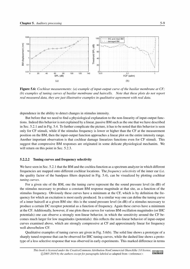
A more precise picture is provided by the so-called input-output functions of the basilar membrane,which are defined as follows: for a given site of the BM the input-output function represents the BMvelocity (or displacement) as a function of sound pressure level (in dB) of the stimulus, and with stimulusfrequency as a parameter. Figure 5.6(a) provides a qualitative example of an input-output function fora CF stimulus. Interestingly this plot shows that responses to stimuli with frequencies near CF exhibita highly compressive growth, i.e., response magnitude grows less than linearly. Compression is mostprominent at moderate and high stimulus intensities, while at low intensities the dependence is almostlinear. There is some evidence that the curve switch back to a linear dependence also for very highstimulus frequencies (around 100 dB, although some data suggest that linearization starts somewhatearlier, at 80− 90 dB).
The highly compressive behavior of input-output functions for BM responses at frequencies aroundCF allows the cochlea to translate the enormous range (120 dB) of auditory stimuli into a range ofvibrations (30 − 40 dB) suitable for transduction by the inner hair cells which have a narrow dynamicrange. This behavior probably provides the foundation of many psychoacoustic phenomena that we willexamine in Sec. 5.3, such as the nonlinear growth of forward masking with masking level and the level
This book is licensed under the CreativeCommons Attribution-NonCommercial-ShareAlike 3.0 license,c⃝2005-2019 by the authors except for paragraphs labeled as adapted from <reference>
Chapter 5. Auditory processing 5-9
0 20 40 60 80 100 120 1400.01
0.1
1
10
100
1000
SPL (dB)
BM
dis
pla
cem
ent (n
m)
(a)
0.01 0.1 10
20
40
60
80
100
f/CF (adim)
Thre
shold
SP
L (
dB
)
IHC and intact BM
damaged BM
(b)
Figure 5.6: Cochlear measurements: (a) example of input-output curve of the basilar membrane at CF;(b) examples of tuning curves of basilar membrane and haircells. Note that these plots do not reportreal measured data, they are just illustrative examples in qualitative agreement with real data.
dependence in the ability to detect changes in stimulus intensity.But before that we need to find a physiological explanation to the non-linearity of input-output func-
tions. Indeed this behavior is not explained by a linear, passive BM such as the one that we have describedin Sec. 5.2.1 and in Fig. 5.4. To further complicate the picture, it has to be noted that this behavior is seenonly for CF stimuli, while if the stimulus frequency is lower or higher than the CF at the measurementposition on the BM, then the input-output function approaches a linear plot on the entire intensity range.Another important observation is that cochlear damage linearizes functions even for CF stimuli. Thissuggest that compressive BM responses are originated in some delicate physiological mechanim. Wewill return on this point in Sec. 5.2.3.
5.2.2.2 Tuning curves and frequency selectivity
We have seen in Sec. 5.2.1 that the BM and the cochlea function as a spectrum analyzer in which differentfrequencies are mapped onto different cochlear locations. The frequency selectivity of the inner ear (i.e.the quality factor of the bandpass filters depicted in Fig. 5.4), can be visualized by plotting cochleartuning curves.
For a given site of the BM, one the tuning curve represent the the sound pressure level (in dB) ofthe stimulus necessary to produce a constant BM response magnitude at that site, as a function of thestimulus frequency. Obviously these curves have a minimum at the CF, which is by definition the fre-quency for which an excitation is most easily produced. In a similar way one can define the tuning curveof a inner haircell at a given BM site: this is the sound pressure level (in dB) of a stimulus necessary toproduce a certain DC receptor potential as a function of frequency. Again these curves have a minimumat the CF. Additionally, however, if one plots these curves for various BM oscillation magnitudes (or IHCpotentials) one can observe a strongly non-linear behavior, in which the sensitivity around the CF be-comes much larger for low magnitudes (potentials): this reflects the non-linear behavior of input-outputcurves examined above, which are strongly compressive at CF and approximately linear for frequencywell above/below CF.
Qualitative examples of tuning curves are given in Fig. 5.6(b). The solid line shows a prototype of asharply tuned response that can be observed for IHC tuning-curves, while the dashed line shows a proto-type of a less selective response that was observed in early experiments. This marked difference in terms
This book is licensed under the CreativeCommons Attribution-NonCommercial-ShareAlike 3.0 license,c⃝2005-2019 by the authors except for paragraphs labeled as adapted from <reference>
5-10 Algorithms for Sound and Music Computing [v.February 2, 2019]
of selectivity between the two curves was taken by many researchers to imply the presence of some sortof “second filter” between the BM and the afferent nerve, a mechanism that was supposed to transformpoorly tuned and insensitive mechanical vibrations into well-tuned and sensitive IHC responses.
However, later in vivo measurements on intact BMs have not confirmed this conjecture, since theyhave provided evidence that BM tuning curves are at least comparable to those of IHCs and that sharptuning observed in IHC responses is present in the BM mechanics as well. In retrospect, it seems apparentthat early methods for the measurement of BM vibrations induced severe physiological damage in thecochlea. However these later findings raise the question of how this mechanical behavior with sharptuning is achieved. The linear passive cochlea such as that of Fig. 5.4 does not seem to be able toproduce a similar performance.
It has to be noted that all the measures related to input-output functions and to tuning curves areobtained as responses to sinusoidal signals. If the cochlea were a linear system these measures wouldprovide all the information that is needed to characterize its behavior. However, as we are starting tounderstand, the cochlea is a non-linear system and thus these responses cannot generally be used topredict responses to arbitrary stimuli. Therefore many studies of BM behavior also use other stimuli,such as tone complexes, noise, and clicks.
5.2.2.3 Two-tone interactions
Psychophysical studies on two-tone interactions led to a recognition of the existence of BM nonlinearitieswell before these were demonstrated in physiological experiments. In this brief section we anticipatesome psychoacoustic studies, which will be further discussed in Sec. 5.3.
Two-tone suppression consists of the reduction of the audibility of one sinusoidal probe tone bythe simultaneous presence of a second, suppressor tone. This psychophysical evidence has a directphysiological counterpart in BM behavior. Specifically, if we look at BM response at a given site (i.e.at a certain CF) and apply a probe tuned to the CF plus a suppressor, the following behavior can beobserved: for zero or low suppressor levels the input-output functions grow as usual at compressiverates. At higher suppressor levels however, the responses to low-level CF tones are reduced strongly,but only weakly at high levels. As a result, the BM input-output curve for the CF tones is substantiallylinearized in the presence of moderately intense suppressor tones.
Tuning curves are also affected by the two-tone suppression phenomenon. If we look at BM responseat a given site and apply a probe with varying frequencies plus a suppressor, the following behavior canbe observed: the tuning curve exhibits a reduced selectiviy, so that the magnitude of suppression isin general maximal at CF and diminishes as the frequency of the probe tones departs from CF. Butsuppression is also CF specific in that, with a fixed probe tone at CF, suppression thresholds vary muchin the same manner as the sensitivity of BM responses to single tones, i.e., suppression thresholds arelowest for suppressor frequencies close to CF.
A second relevant phenomenon that points to the existence of BM nonlinearities is intermodulationdistortion. We have examined in Chapter Sound modeling: signal based approaches the concept of memorylessnonlinear processing, and the generation of intermodulation frequencies when a linear combination ofsinusoidal signals is passed through a nonlinear distortion function. This phenomenon is in fact observedin the BM: when two (or more) sinusoidal signals are presented simultaneously, humans can hear addi-tional frequencies that are not actually present in the acoustic stimulus. In the case of two-tone stimuli,the additional tones have frequencies corresponding to combinations of the two original sinusoidal fre-quencies (f1 and f2 > f1), such as f2 − f1, 2f1 − f2, 2f2− f1. Additionally, their perceived intensityis highly dependent on stimulus-frequency separation.
Again, this psychophysical evidence has a direct counterpart in the mechanics of the cochlea: ex-periments have demonstrated the presence of distortion products in BM vibrations. BM responses to
This book is licensed under the CreativeCommons Attribution-NonCommercial-ShareAlike 3.0 license,c⃝2005-2019 by the authors except for paragraphs labeled as adapted from <reference>

Chapter 5. Auditory processing 5-11
two-tone stimuli with close frequencies contain several distortion products, or difference tones, at fre-quencies both higher and lower than the frequencies of the primary tones (3f2 − 2f1, 2f2 − f1, 2f1 −f2, 3f1 − 2f2, f2 − f1, . . .). As f1, f2 are increasingly separated, the number of detectable distortionproducts in the response decreases.
So-called cubic difference tones (2f1−f2) are particularly relevant. Psychophysical experiments withhuman subjects show that these tones reach levels as high as −15 dB to −22 dB relative to the level ofthe primaries. Moreover, for equal-level primaries distortion product magnitudes grow at linear or faster-than-linear rates at low intensities, and saturate and even decrease slightly at higher stimulus intensities(≥ 60 dB). In general relative levels of distortion-products are highest at low stimulus intensities anddecrease little over wide ranges of stimulus intensity. For a fixed level of one of the primary tones,the distortion product magnitude is a nonmonotonic function of the level of the other primary tone.For moderate f2/f1 ratios (e.g., > 1.2), distortion product magnitudes decrease rapidly with increasingfrequency ratio.1
Two-tone distortion is also CF specific, in that the magnitude and phase of distortion products on theBM depend strongly on the frequency separation between the primary tones. The magnitude of the cubicdifference tone on the BM decays with increasing frequency ratio.
5.2.3 Active amplification in the cochlea
Nowadays it is generally accepted that many properties of auditory nerve responses probably reflectcorresponding features of BM vibration, including sharp frequency tuning, compressive input-outputnon-linearity at near-CF frequencies, two-tone suppression and distortion. Appropriately, all these prop-erties exhibit CF specificity, i.e., a dependency on stimulus frequency relative to CF, while many otherproperties of auditory nerve responses do not exhibit CF specificity and, accordingly, probably originateat sites other than the BM (such as IHCs and their synapses).
The problem is then to explain how the BM can exhibit these properties. In contemporary research,the dominant explanation takes the name of cochlear amplification. This definition indicates some sort ofpositive feedback to BM vibrations in which biological energy is converted into mechanical vibrations,with the effect of increasing sensitivity of BM responses, in particular to low-level stimuli, and frequencyselectivity. This is obtained at the expense of dissipation of biological energy (i.e., not present in theacoustic stimulus).
5.2.3.1 Experimental evidence for cochlear amplification
In Sec. 5.2.2 we have reviewed non-linear behaviors at cochlear sites. At least at the base of the cochlea,compressive non-linearity, high sensitivity, and sharpness of frequency tuning appear to be inextricablylinked with each other: when one of these three properties is abolished by cochlear insults the other twoare also eliminated or drastically reduced.
The most permanent cochlear damage is death: various measurements have shown that post-mortemcochlear responses exhibit disappearance of compressive non-linearity, loss of sensitivity, and broaden-ing of tuning curves, accompanied by a downward shift (up to one-half octave) of the most sensitivefrequency (see Fig. 5.6(b)). Surgical trauma and exposure to intense sounds are other source of cochleardamage: in particular the effects of acoustic overstimulation on BM responses closely resembles the
1Italian composer, violinist, and music theorist Giuseppe Tartini is credited with the discovery of difference tones. Inparticular the “terzo suono di Tartini” (Tartini’s third sound) can be heard when playing two violin strings tuned at a perfectfifth, say f1 and f2 = 3/2f1: in this case the quadratic (f2 − f1) and cubic (2f1 − f2) distortion products both give 1/2f1,and a listener perceives a tone one octave lower than f1.
This book is licensed under the CreativeCommons Attribution-NonCommercial-ShareAlike 3.0 license,c⃝2005-2019 by the authors except for paragraphs labeled as adapted from <reference>

5-12 Algorithms for Sound and Music Computing [v.February 2, 2019]
effects of death. In some cases (e.g., listening to a few rock concerts) the effects can be transient, whilein other cases (e.g., listening to a few more rock concerts) they can be permanent.
Measurements on damaged cochleae point to the existence of some delicate cellular process thatboost BM vibrations, but do not address directly the nature of this process. More indications are pro-vided by experiments that manipulate cochlear responses via pharmacological means, in particular usingsubstances that drastically but reversibly alter cochlear function by abolishing the endocochlear potential.This reduces the drive to mechanoelectrical transduction, presumably causing reduced receptor poten-tials of haircells, and ultimately altering the sensitivity of auditory nerve fibers. These experiments showthat changes in high-CF fiber responses are substantially greater at CF than at other frequencies. Thisimplies that the sensitivity and non-linearity of BM vibrations depend critically on the receptor potentialsof haircells, and that the cochlear amplification mechanism is associated with some sort of feedback fromthe organ of Corti to BM vibration.
One further step towards the localization of the cochlear amplification mechanism is provided by ex-periments on electrical stimulation of efferent fibres (which as we know terminate at the base of OHCs).These experiments clearly show that efferent fibers have an inhibitory effect on cochlear responses: inparticular, CF-specific loss of sensitivity and linearization of BM vibrations is observed. This is a strongindicator of the ability of OHCs to influence BM vibrations. Because it is inconceivable that afferentfibers can affect BM vibrations, the efferent effects must be mediated by OHCs.
Another striking phenomenon that suggests that biological energy can be converted into cochlearvibrations is the existence of spontaneous otoacoustic emissions. Otoacoustic emissions are in generaldefined as sounds produced inside the auditory system, and can be measured in the ear canal using verysensitive microphones, since their level is extremely small.2 Spontaneous emissions in particular arenarrow-band sounds emanating continuously from the inner ear in the absence of acoustic stimulation.They are often understood to represent oscillations powered by biological energy sources. Because thereis some indirect evidence that spontaneous emissions are accompanied by corresponding BM vibrations,one can venture to postulate that the same processes that give rise to spontaneous emissions are alsoinvolved in amplifying the magnitude of acoustically stimulated BM motion.
5.2.3.2 Reverse transduction and OHC electromotility
The biological energy that is supposedly converted into mechanical energy is presumably electrical.Therefore if cochlear amplification actually takes place, there must be some mechanism for reverse,electrical-to-mechanical transduction in the cochlea.
This conjecture is supported by experimental evidence. Direct currents passed across the organ ofCorti produce marked changes in BM responses to acoustic stimuli with frequencies at and above CF, andlittle changes in responses to stimuli with frequencies below CF. Positive currents (from scala vestibulito scala tympani) increase the sensitivity and frequency tuning of BM sound-evoked motion and shiftits characteristic frequency upward, while negative currents decrease the sensitivity and tuning of theresponse and shift the characteristic frequency downward. Presumably, the effects of negative currentsare analogous to those of decreased endocochlear potential obtained through pharmacological means (asdiscussed above).
Another finding is that when sinusoidal currents are injected into the scala media and an acousticstimulus is simultaneously delivered, otoacoustic emissions are evoked. More precisely, the sinusoidalcurrent generates emissions with the same frequency of the electrical stimulus, and also interacts with
2Here we mention otoacoustic emissions briefly only to the extent that they shed direct light on active cochlear vibrations.The reader should be aware that this is a diversified phenomenon that includes spontaneous emissions produced without a soundstimulus, simultaneously evoked emissions during tonal stimulation, delayed evoked emissions in response to periodic impulses(e.g., broad-band clicks), and distortion product emissions produced by stimulation with two primaries.
This book is licensed under the CreativeCommons Attribution-NonCommercial-ShareAlike 3.0 license,c⃝2005-2019 by the authors except for paragraphs labeled as adapted from <reference>

Chapter 5. Auditory processing 5-13
of basilarVibration
Deflectionof
stereocilia
OHCmotion
Acousticstimulus
currentmodulation
fromIHCs
Spikes
OHC
membrane
D B
A
C
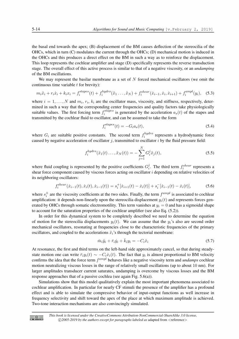
Figure 5.7: Schematic representation of the positive feedback that causes cochlear amplification. TheOHCs are involved in the loop while IHCs have no role in the amplification and are passive motiondetectors .
the acoustic tone to produce distortion-product otoacoustic emissions. These findings support the idea ofelectrically induced BM motion, and indeed some in vivo experiments have also directly demonstratedthe existence of electrically induced BM motion for some mammalian cochleae.
One of the most authoritative candidates to explain reverse transduction is the so-called phenomenonof somatic electromotility in OHCs. This definition refers to the ability of OHCs to exhibit rapid motileresponses, namely elongation and shortening, in response to hyperpolarization or depolarization of theirtransmembrane potential. Depolarization causes outer haircells to shorten, pulling the reticular laminatoward the scala tympani, and the BM toward the scala vestibuli. Hyperpolarization instead causes rapidelongation of OHCs. Intrinsically, such responses are sufficiently fast to provide forces (or stiffnesschanges) potentially capable of enhancing BM vibration, on a cycle-by-cycle basis, even at the highest-CF regions of the cochlea.
The channel conductivity S of OHCs depends non-linearly upon stereocilia deflection, so that thevoltage-displacement relation exhibits compression and saturation and resembles a second-order Boltz-mann function:
S(y) =1
1 + c1e−y/y1 + c2e−y/y2− b, (5.2)
where y is a quantity proportional to stereocilia deflection, scaled by a coefficient that depends uponposition along the BM. All coefficients can be determined in order to fit physiological data. The sigmoidshape of this function implies that the motile responses of OHCs ceases to be effective outside a narrowrange of stereocilia deflection.
5.2.3.3 The cochlear amplifier at work
If the mechanical feedback that the organ of Corti exerts upon BM vibration is controlled by the mag-nitude of haircell receptor potentials or transduction currents, the non-linear nature of this transductionprocess must necessarily result in mechanical counterparts in BM vibration. Accordingly, models in-corporating a feedback loop between OHCs and BM vibration often identify reverse transduction as thesource of all BM non-linear phenomena, including the compressive growth at CF, as well as two-tonesuppression and intermodulation distortion.
We can summarize the whole idea of the cochlear amplifier as in Fig. 5.7: (A) acoustic power enteringthe cochlea induces a pressure difference across the BM and a traveling wave motion that propagates from
This book is licensed under the CreativeCommons Attribution-NonCommercial-ShareAlike 3.0 license,c⃝2005-2019 by the authors except for paragraphs labeled as adapted from <reference>
5-14 Algorithms for Sound and Music Computing [v.February 2, 2019]
the basal end towards the apex; (B) displacement of the BM causes deflection of the stereocilia of theOHCs, which in turn (C) modulates the current through the OHCs; (D) mechanical motion is induced inthe OHCs and this produces a direct effect on the BM in such a way as to reinforce the displacement.This loop represents the cochlear amplifier and stage (D) specifically represents the reverse transductionstage. The overall effect of this active process is similar to that of a negative viscosity, or an undampingof the BM oscillations.
We may represent the basilar membrane as a set of N forced mechanical oscillators (we omit thecontinuous time variable t for brevity):
mixi + rixi + kixi = fstapesi (t) + fhydro
i (x1 . . . , xN ) + fsheari (xi−1, xi, xi+1) + fampl
i (yi), (5.3)
where i = 1, . . . , N and mi, ri, ki are the oscillator mass, viscosity, and stiffness, respectively, deter-mined in such a way that the corresponding center frequencies and quality factors take physiologicallysuitable values. The first forcing term f stapes
i is generated by the acceleration as(t) of the stapes andtransmitted by the cochlear fluid to oscillator, and can be assumed to take the form
f stapesi (t) = −Gias(t), (5.4)
where Gi are suitable positive constants. The second term fhydroi represents a hydrodynamic force
caused by negative acceleration of oscillator j, transmitted to oscillator i by the fluid pressure field:
fhydroi (x1(t) . . . , xN (t)) = −
N∑j=1
Gji xj(t), (5.5)
where fluid coupling is represented by the positive coefficients Gji . The third term f shear
i represents ashear force component caused by viscous forces acting on oscillator i depending on relative velocities ofits neighboring oscillators:
fsheari (xi−1(t), xi(t), xi−1(t)) = s+i [xi+1(t)− xi(t)] + s−i [xi−1(t)− xi(t)], (5.6)
where s±i are the viscosity coefficients at the two sides. Finally, the term fampl is associated to cochlearamplification: it depends non-linearly upon the stereocilia displacement yi(t) and represents forces gen-erated by OHCs through somatic electromotility. This term vanishes at yi = 0 and has a sigmoidal shapeto account for the saturation properties of the cochlear amplifier (see also Eq. (5.2)).
In order for this dynamical system to be completely described we need to determine the equationof motion for the stereocilia displacements yi(t). We can assume that the yi’s also are second ordermechanical oscillators, resonating at frequencies close to the characteristic frequencies of the primaryoscillators, and coupled to the accelerations xi’s through the tectorial membrane:
miyi + riyi + kiyi = −Cixi (5.7)
At resonance, the first and third terms on the left-hand side approximately cancel, so that during steady-state motion one can write riyi(t) ∼ −Cixi(t). The fact that yi is almost proportional to BM velocityconfirms the idea that the force term fampl behaves like a negative viscosity term and undamps cochlearmotion neutralizing viscous losses in the range of relatively small oscillations (up to about 10 nm). Forlarger amplitudes transducer current saturates, undamping is overcome by viscous losses and the BMresponse approaches that of a passive cochlea (see again Fig. 5.6(a)).
Simulations show that this model qualitatively explain the most important phenomena associated tocochlear amplification. In particular for nearly CF stimuli the presence of the amplifier has a profoundeffect and is able to simulate the compressive behavior of input-output functions as well increase infrequency selectivity and shift toward the apex of the place at which maximum amplitude is achieved.Two-tone interaction mechanisms are also convincingly simulated.
This book is licensed under the CreativeCommons Attribution-NonCommercial-ShareAlike 3.0 license,c⃝2005-2019 by the authors except for paragraphs labeled as adapted from <reference>

Chapter 5. Auditory processing 5-15
5.3 Elements of psychoacoustics
We still know very little about how sensorial stimuli are processed in the brain: this is why resultsfrom psychophysics are useful. Psychophysics investigates quantitative relationships between physicalstimuli and the sensations and perceptions that they produce. Generally speaking, psychophysical studiesanalyze perceptual processes by investigating how systematic variations of the properties of a sensorialstimulus along one or more physical dimensions affect the experience or the behaviour of a humanperceiver.
Quantitative results from psychophysics have produced a range of important practical applicationsemploying computational models of human perception. A typical example is the development of modelsand methods of perceptual compression in the field of digital signal processing: these models producelossy compression algorithms that allow for high compression rates at the expense of little or null loss ofperceived quality.
As a branch of psichophysics, psychoacoustics is concerned with the study of auditory perception.This section summarizes some fundamental aspects, focusing on what may be termed “engineering psy-choacoustics”: quantitative results that are the basis for the development of computational models ofauditory functions.
5.3.1 Loudness
Loudness can be defined as that attribute of auditory sensation that corresponds most closely to thephysical measure of sound intensity, or as a psychological description of the magnitude of an auditorysensation. As we will see the loudness of a sound strongly depends on both the sound intensity and itsfrequency content.
5.3.1.1 Threshold in quiet
In Chapter Fundamentals of digital audio processing we have defined sound pressure level and the related dB unitas
SPL = 10 log10(I/I0) = 20 log10(p/p0) (dB), (5.8)
where I and p are the RMS intensity and acoustic pressure of the sound signal, respectively, while I0 andp0 are a reference intensity and a reference pressure, respectively. In particular, in an absolute dB scale I0and p0 are chosen to be the intensity and the pressure at the threshold of hearing and have conventionallythe values I0 = 10−12 W/m2 and p0 = 2 · 10−5 Pa, respectively. A dB scale that uses these referencevalues is often indicated with the unit dBSPL.
However these values are only qualitative indicators of the true threshold of hearing. In particularthey do not consider that this threshold is frequency-dependent. The most typical experimental setup usedto measure the treshold of hearing in quiet is the following: a subject listen to a sweep signal in which thefrequency is changing very slowly. As the sweep frequency changes, the subject can continuously adjustthe volume in such a way that he/she maintains the tone around the threshold of audibility. This methodis known as the “Bekesy-tracking” method (from the name of its inventor), and the resulting trajectoriesof increments-decrements in volume will typically produce a plot like the one in Fig. 5.8(a).
This plot is an estimate of the threshold sound pressure level in quiet. Although a specific plot isproduced by a specific subject, the dependence on frequency is qualitatively similar in many subjectswith normal hearing. At low frequencies, threshold in quiet requires pretty high SPLs (as much as40 dB around 50 Hz). For frequencies in the range 0.5 − 2 kHz, the threshold in quiet remains almostindependent of frequency. The range 2 − 5 kHz is a very sensitive range in which very small SPLs(even below 0 dB) are perceived. Above 5 kHz, the threshold exhibits peaks and valleys that vary greatly
This book is licensed under the CreativeCommons Attribution-NonCommercial-ShareAlike 3.0 license,c⃝2005-2019 by the authors except for paragraphs labeled as adapted from <reference>

5-16 Algorithms for Sound and Music Computing [v.February 2, 2019]
102
103
104
−20
0
20
40
60
80
100
Frequency (Hz)
Sou
nd p
ressure
level (d
B)
(a)
102
103
104
0
20
40
60
80
100
120
10
20
30
40
50
60
70
80
90
100 phons
Frequency (Hz)
Sou
nd p
ressure
level (d
B)
(b)
Figure 5.8: Loudness formation; (a) threshold in quiet as a function of frequency, measured with themethod of Bekesy-tracking; (b) equal loudness contours illustrating the variation in loudness with fre-quency (each curve represents one loudness level).
depending on the subject, but in general it increases rapidly for frequencies above 12 kHz and finallyreaches a limit above which no sensation is produced even at very high SPLs. This limit is stronglydependent on the age of the subject: it is roughly in the range 16− 18 kHz for an age of 20− 25 years,and drops with increasing age.
Using individual thresholds in quiet measured in many subjects, an average threshold in quiet can becalculated. The dashed curve in Fig. 5.8(a) indicates such an averaged curve. One possible parametriza-tion of this curve is given by the equation
pth(f) = 3.64
(f
1000
)−0.8
− 6.5e−0.6( f1000
−3.3)2
+ 103(
f
1000
)4
(dB SPL). (5.9)
5.3.1.2 Equal loudness contours and loudness scales
Equal loudness contours describe the frequency dependence of the loudness of sinusoidal tones. Thesecurves are typically measured by requiring listeners to match the intensity of a comparison sinusoid ofvariable frequency to the intensity of a reference sinusoid at 1 kHz.
Many experiments have been carried out to determine equal loudness contours along the audiblerange of hearing, and many investigators have reported qualitatively similar results, although with somequantitative differences. Figure 5.8(b) shows equal loudness contours as reported in some of the mostrecent studies, which have contributed to the latest version of the international standard ISO 226:2003(Acoustics – Normal equal-loudness-level contours). Although the curves tend to follow the absolutethreshold curve at low loudness levels, it can be seen that at high loudness levels the contours flattensomewhat. This phenomenon is experienced in everyday life when listening to recorded music: a greaterrelative amount of bass is perceived at high intensities than at low intensities.
Starting from the 1950’s, several analytical approximations of these curves have been proposed. Ifone considers loudness of sinusoidal sounds with a fixed frequency and variable intensity, at moderateto high sound pressure levels the growth of loudness is well approximated by the power law S = ap2α,where p is the acoustic pressure of the sinusoid, a is a dimensional constant, α is the exponent, and S
This book is licensed under the CreativeCommons Attribution-NonCommercial-ShareAlike 3.0 license,c⃝2005-2019 by the authors except for paragraphs labeled as adapted from <reference>

Chapter 5. Auditory processing 5-17
is the perceived loudness. However this approximation cannot describe the dependence of loudness onfrequency, nor the deviation of the loudness function from power-law behavior below about 30 dB. Onerecently proposed modification to the power-law (which has been used to plot Fig. 5.8(b)), assumes inparticular frequency-dependent parameters a(f) and α(f)
p2(f) =1
u2(f)
{[p(1000)2α(1000) − pth(1000)
2α(1000)]+ [u(f)pth(f)]
2α(f)}1/α(f)
, (5.10)
where u(f) = [a(f)/a(1000)]1/2α(f) (therefore u(1000) = 1). The meaning of this equation is thefollowing: the loudness of a sinusoid with frequency f is equal to the loudness of a reference 1 kHzsinusoid (with acoustic pressure p(1000)), when its acoustic pressure is p(f). Note that at threshold thethe value p(f) coincides with pth(f), as one would expect.
For a given reference value p(1000), an equal loudness contour p(f) can be drawn if the functionsa(f) and α(f) (or equivalently u(f) and α(f)) are known, i.e. estimated from experimental data. Thefollowing function computes Eq. (5.10) using experimental values reported in recent literature.
M-5.1Write a function that an equal loudness contour p(f), given a reference acoustic pressure p(1000).
M-5.1 Solution
function [spl, f] = eqloudness(db); %db: reference pressure at 1kHz, in dB
p0=2E-5; %standard acoustic pressure at threshold of sensitivityalpha1=0.25; %value of exponent alpha at reference freq. 1kHzpth1= (1.15)ˆ(1/(2*alpha1))*p0; %threshold acoustic pressure at 1kHz
%...from the equality (prt/p0)ˆ2alpha1=1.15
%%%%%%%%%%%%%%%%%%%%% frequency-dependent parameters %%%%%%%%%%%%%%%%%%%%%%%%%%
f =[20 25 31.5 40 50 63 80 100 125 160 200 250 315 400 500 630 800 1000 1250 ...1600 2000 2500 3150 4000 5000 6300 8000 10000 12500]; %%%% frequency points
alphaf = [0.532 0.506 0.480 0.455 0.432 0.409 0.387 0.367 0.349 0.330 0.315 ...0.301 0.288 0.276 0.267 0.259 0.253 0.250 0.246 0.244 0.243 0.243 ...0.243 0.242 0.242 0.245 0.254 0.271 0.301]; %%%% exponent alpha(f)
logu = [-31.6 -27.2 -23.0 -19.1 -15.9 -13.0 -10.3 -8.1 -6.2 -4.5 -3.1 ...-2.0 -1.1 -0.4 0.0 0.3 0.5 0.0 -2.7 -4.1 -1.0 1.7 ...2.5 1.2 -2.1 -7.1 -11.2 -10.7 -3.1]; %%%% coefficient u(f)
uf =2*10.ˆ(logu/20-5); %...from the equality 0.4*10ˆ(log(u(f))/10 -9) = u(f)ˆ2;
dB_pthf = [ 78.5 68.7 59.5 51.1 44.0 37.5 31.5 26.5 22.1 17.9 14.4 ...11.4 8.6 6.2 4.4 3.0 2.2 2.4 3.5 1.7 -1.3 -4.2 ...-6.0 -5.4 -1.5 6.0 12.6 13.9 12.3];
pthf=10.ˆ(dB_pthf/20); %%%% freq.-dependent threshold acoustic pressure p_th(f)
%%%%%%%%%%%%%%%%%%%%%%%%%%%%%%%%%%%%%%%%%%%%%%%%%%%%%%%%%%%%%%%%%%%%%%%%%%%%%%
p1 =p0*10ˆ(db/20); %reference press. at 1kHz, from equality db= 20*log10(pr/p0)pf2=uf.ˆ-2.*(p1ˆ(2*alpha1)-pth1ˆ(2*alpha1)+(uf.*pthf).ˆ(2*alphaf)).ˆ(1./alphaf);spl= 10*log10(pf2);
This book is licensed under the CreativeCommons Attribution-NonCommercial-ShareAlike 3.0 license,c⃝2005-2019 by the authors except for paragraphs labeled as adapted from <reference>

5-18 Algorithms for Sound and Music Computing [v.February 2, 2019]
102
103
104
−60
−50
−40
−30
−20
−10
0
10
Frequency (Hz)
Mag
nitud
e (
dB
)
Figure 5.9: A-weighted dB scale: (a) inverse curve of the 40 phon equal loudness contour, and (b)magnitude response of the filter HdBA(s), digitized with the bilinear transform.
Using equal loudness contours, one can define a psychophysical scale of loudness, whose unit ofmeasure is the phon. The loudness level in phons of a sinusoid at frequency f is defined as the level (indB SPL) of the 1 kHz tone that produces that same perceived loudness. As an example, any tone that hasthe same loudness of a 60 dB, 1 kHz tone has, by definition, a loudness of 60 phons.
However the phon unit only describes sounds that are equally loud, while it cannot be used to measurerelationships between sounds with different loudness. As an example, a sinusoid at 40 phons is not twiceas loud as a sinusoid at 20 phons. In fact, psychophysical experiments show that an increase of 10 phonsapproximately produce the impression of loudness doubling. Starting from this observation, the sonescale of subjective loudness can be introduced. One sone is arbitrarily defined to correspond to 40 phonsat any frequency. A sinusoid that is judged by listeners to be twice as loud as the 1 sone sinusoid will bedefined to have a loudness of 2 sones. Therefore, in light of the above observation, 2 sones correspondto 50 phons. Similarly, 4 sones are twice as loud again, i.e. they correspond to 60 phons. Therefore therelationship between phons and sones is expressed by the equation
phon = 40 + 10 log2(sone). (5.11)
5.3.1.3 Weighting curves
Since equal loudness contours are not flat, plotting the spectrum of a sound signal (either on a linear scaleor on the dB SPL scale) does not represent very accurately our perception of that spectrum. In particular,we have seen that humans are most sensitive to spectral energy in the frequency range from 0.5 to 5 kHz,while they are less sensitive to spectral energy in the low- and high-frequency ranges.
In order to produce a more perceptually relevant spectral representation of a sound, a common pro-cedure is to pass the sound signal through a filter that compensates for non-flat equal loudness contours.Two remarks need to be made: first, the shape of equal loudness contours changes with loudness; sec-ond, the loudness of a sound with a complex spectrum is not obtained by summing the loudness of eachof its sinudoidal components, due to the non-linear behavior of our auditory system (we will return onthis point in the next section). Therefore a linear filtering operation cannot in principle produce an ac-curate loudness compensation. Having said that, linear filtering is nonetheless used in many practicalapplications.
One of the most commonly used weighting filters corresponds to the so-called A-weighted dB scale(usually abbreviated as dBA). The magnitude response of this filter approximates the inverse of the equalloudness contour at 40 phons. Therefore a dBA weighting is only accurate for fairly quiet sinusoidal
This book is licensed under the CreativeCommons Attribution-NonCommercial-ShareAlike 3.0 license,c⃝2005-2019 by the authors except for paragraphs labeled as adapted from <reference>

Chapter 5. Auditory processing 5-19
sounds. Despite this, this weighting is often used as an approximate equal loudness adjustment forany measured spectra. An analog filter transfer function that can be used to implement an approximateA-weighting is
HdBA(s) =(2π · 13682)2s4
(s+ 2π · 20.6)2(s+ 2π · 107.7)(s+ 2π · 737.9)(s+ 2π · 12194.2)2, (5.12)
where the coefficient at the numerator normalizes the gain to unity at 1 kHz. Figure 5.9 illustratesthe magnitude response of a digital filter HdBA(z) (obtained by digitizing Eq. (5.12) with the bilineartransform) and compares it with the inverse curve of the equal loudness contour at 40 phons.
M-5.2Write a function that computes the coefficients of a digital filter approximating the A-weighted dB scale with thebilinear tranform.
M-5.2 Solution
function [b,a]= compute_Aweight();
global Fs;
k = 2*pi*13681.8653719;p1 = -2*pi*20.598997; p2 = -2*pi*12194.217;p3 = -2*pi*107.65265; p4 = -2*pi*737.86223;
[bil_zeros,bil_poles,bil_k]=bilinear([0;0;0;0],[p1;p1;p2;p2;p3;p4],kˆ2,Fs);[b,a]=zp2tf(bil_zeros,bil_poles,bil_k);
This function has been used to plot the magnitude response in Fig. 5.9.
The A-weighted dB scale has two main drawbacks. First, as already mentioned, it is designed towork at low sound pressure levels. Second and more important, it is based on old and fairly inaccurateexperimental data about equal loudness contours. Other frequency weightings (in particular, B- C- D-weightings) have been proposed. While B- and D-frequency-weightings have fallen into disuse, theC-frequency-weighting is still widely used.
5.3.2 Masking
In the previous section we have examined the perception of loudness of single sound in quiet conditions.We now consider situations in which two competing sounds are heard.
The phenomenon of masking may be simply summarized with the common-sense statement that“a loud sound makes a weaker sound imperceptible”. In fact masking effects are encountered in oureveryday life: when we are speaking to another person, we need little speech power in quiet conditions,while the conversation is severely disturbed in the presence of a masker signal (e.g. if we are speakinginside a noisy bus) and we will probably have to raise our voice to produce more speech power andgreater loudness. Similarly, the sound of one orchestral instrument may be made imperceptible by thatof another instrument, if one is very loud while the other remains soft.
Quantitative measures of masking are devoted to the determination of the masking threshold, i.e. thesound pressure level of a probe signal (usually a sinusoidal signal) that is needed to make it just audiblein the presence of a masker signal. If the level of the masker signal is increased steadily, a continuoustransition between a perfectly audible and a totally masked probe signal will occur, and partial masking
This book is licensed under the CreativeCommons Attribution-NonCommercial-ShareAlike 3.0 license,c⃝2005-2019 by the authors except for paragraphs labeled as adapted from <reference>

5-20 Algorithms for Sound and Music Computing [v.February 2, 2019]
102
103
104
0
20
40
60
80
100
f (Hz)
SP
L (
dB
)
Lmask
40
−10
0
10
20
30
10 dB per decade
= 50 dB
(a)
102
103
104
0
20
40
60
80
100
f (Hz)
SP
L (
dB
)
Lmask dB40=
low−pass noisehigh−pass noise
20
0
(b)
Figure 5.10: Masking threshold curves of a sinusoidal probe signal as a function of its frequency; (a)masking caused by white noise with density levels Lmask; (b) masking caused by 1.1 kHz low-passfiltered white noise and 0.9 kHz high-pass filtered white noise with density levels Lmask. Here and in thefollowing figures the dashed curve indicates threshold of hearing in quiet (see Sec. 5.3.1).
will occur in between. Partial masking reduces the loudness of a probe signal but does not mask itcompletely. This effect often takes place in conversations.
These masking effects are example of simultaneous masking, i.e. they can be observed when maskerand probe signals are presented simultaneously. However masking can also occur when they are notsimultaneous. In particular, when the probe is a sound impulse which is presented right before the maskeris switched on, or right after the masker is switched off, then “premasking” (or “backward masking”) and“postmasking” (or “forward masking”) occur, respectively. In the remainder of this section we discussin detail all these effects.
5.3.2.1 Simultaneous masking: noise-masking-tone
Simultaneous masking is best understood from a frequency-domain point of view: the relative shapesof magnitude spectra of the probe and masker signals determine to what extent the presence of certainspectral energy will mask the presence of other spectral energy (phase relationships between stimulican also affect masking outcomes, although to a lesser extent). As we will see, an explanation of themechanism underlying simultaneous masking phenomena is that the presence of a strong noise or tonalmasker creates an excitation on a certain portion of the basilar membrane which is strong enough toblock effectively the detection of a weaker signal.
A widely studied type of simultaneous masking is the so-called Noise-Masking-Tone (NMT), in whichthe masking signal is a broad- or narrow-band noise and the probe signal is a sinusoid. Ideal white noiseis the most easily defined broad-band noise, its flat spectral density is not associated to any specific pitch.3
Figure 5.10(a) shows the masking threshold curves of a sinusoidal probe in the presence of white noisewith various density levels Lmask, as a function of the sinusoid frequency. The curves are horizontal onlyat low frequencies, and lie about 17 dB above Lmask, while for f > 0.5 kHz they start to rise at a rateof about 10 dB per decade. At very low and very high frequencies the curves will superimpose on thethreshold of hearing in quiet. Note also that the curves depend linearly on Lmask, i.e. increasing Lmask
by a certain number of dB shifts the curves upwards by the same amount. Moreover, even negative values
3In practice, white noise used in auditory research has flat spectral density only in the range from 20 Hz to 20 kHz, whichspans the audible range of hearing.
This book is licensed under the CreativeCommons Attribution-NonCommercial-ShareAlike 3.0 license,c⃝2005-2019 by the authors except for paragraphs labeled as adapted from <reference>
Chapter 5. Auditory processing 5-21
102
103
104
0
20
40
60
80
100
f (Hz)
SP
L (
dB
)
0f = 250 Hz 4 kHz1 kHz
(a)
102
103
104
0
20
40
60
80
100
f (Hz)
SP
L (
dB
)
Lmask
60
80
20
40
100 dB=
(b)
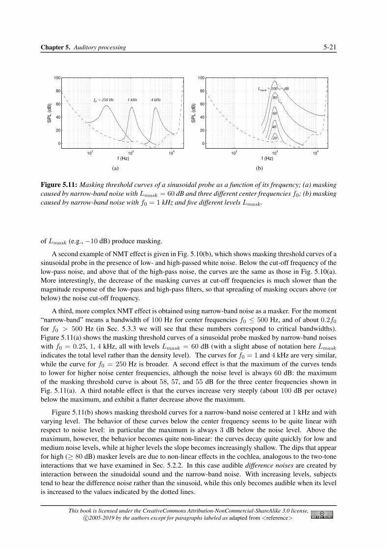
Figure 5.11: Masking threshold curves of a sinusoidal probe as a function of its frequency; (a) maskingcaused by narrow-band noise with Lmask = 60 dB and three different center frequencies f0; (b) maskingcaused by narrow-band noise with f0 = 1 kHz and five different levels Lmask.
of Lmask (e.g., −10 dB) produce masking.
A second example of NMT effect is given in Fig. 5.10(b), which shows masking threshold curves of asinusoidal probe in the presence of low- and high-passed white noise. Below the cut-off frequency of thelow-pass noise, and above that of the high-pass noise, the curves are the same as those in Fig. 5.10(a).More interestingly, the decrease of the masking curves at cut-off frequencies is much slower than themagnitude response of the low-pass and high-pass filters, so that spreading of masking occurs above (orbelow) the noise cut-off frequency.
A third, more complex NMT effect is obtained using narrow-band noise as a masker. For the moment“narrow-band” means a bandwidth of 100 Hz for center frequencies f0 ≤ 500 Hz, and of about 0.2f0for f0 > 500 Hz (in Sec. 5.3.3 we will see that these numbers correspond to critical bandwidths).Figure 5.11(a) shows the masking threshold curves of a sinusoidal probe masked by narrow-band noiseswith f0 = 0.25, 1, 4 kHz, all with levels Lmask = 60 dB (with a slight abuse of notation here Lmask
indicates the total level rather than the density level). The curves for f0 = 1 and 4 kHz are very similar,while the curve for f0 = 250 Hz is broader. A second effect is that the maximum of the curves tendsto lower for higher noise center frequencies, although the noise level is always 60 dB: the maximumof the masking threshold curve is about 58, 57, and 55 dB for the three center frequencies shown inFig. 5.11(a). A third notable effect is that the curves increase very steeply (about 100 dB per octave)below the maximum, and exhibit a flatter decrease above the maximum.
Figure 5.11(b) shows masking threshold curves for a narrow-band noise centered at 1 kHz and withvarying level. The behavior of these curves below the center frequency seems to be quite linear withrespect to noise level: in particular the maximum is always 3 dB below the noise level. Above themaximum, however, the behavior becomes quite non-linear: the curves decay quite quickly for low andmedium noise levels, while at higher levels the slope becomes increasingly shallow. The dips that appearfor high (≥ 80 dB) masker levels are due to non-linear effects in the cochlea, analogous to the two-toneinteractions that we have examined in Sec. 5.2.2. In this case audible difference noises are created byinteraction between the sinudoidal sound and the narrow-band noise. With increasing levels, subjectstend to hear the difference noise rather than the sinusoid, while this only becomes audible when its levelis increased to the values indicated by the dotted lines.
This book is licensed under the CreativeCommons Attribution-NonCommercial-ShareAlike 3.0 license,c⃝2005-2019 by the authors except for paragraphs labeled as adapted from <reference>

5-22 Algorithms for Sound and Music Computing [v.February 2, 2019]
102
103
104
0
20
40
60
80
100
f (Hz)
SP
L (
dB
)
����
����
����������������
����������������
����
����
beating
differencetone
(a)
102
103
104
0
20
40
60
80
100
f (Hz)
SP
L (
dB
)
Lmask
40
= 60 dB
(b)
Figure 5.12: Masking threshold curves of a sinusoidal probe as a function of its frequency; (a) maskingcaused by a sinusoid at 1 kHz and 80 dB, with regions where beats and difference tone are audible; (b)The masked thresholds are given for sound pressure levels of 40 and 60 dB of each partial.
5.3.2.2 Simultaneous masking: tone-masking-noise
5.3.2.3 Simultaneous masking: tone-masking-tone
A second important type of simultaneous masking is the the so-called Tone-Masking-Tone (TMT), inwhich the masker is made of one or more sinusoidal partials, and the probe signal is a sinusoidal sound.Figure 5.12(a) shows an example of masking threshold curve for a sinusoidal probe masked by a sinu-soidal masker. An effect that appears in this case is that beats are audible when the frequencies of theprobe and the masker are close (e.g., a probe at 990 Hz and a masker at 1 kHz produce audible beats at10 Hz), and to a lesser extent in two regions around where the probe frequency is twice or three timesthat of the masker. The example in Fig. 5.12(a) also show that for probe frequencies near 1.4 kHz some(inexperienced) subjects would indicate audibility of an additional tone at a level as low as 40 dB: inreality these subjects would hear a cubic difference tone near 600 Hz (2f1 − f2, with f1 = 1000 Hzand f2 = 1400 Hz) resulting from the two-tone interaction mechanism described in Sec. 5.2.2, while the“true” probe is only detected at higher levels. These results indicate that TMT is in general more difficultto measure than NMT: individual differences are greater, and large numbers of well-trained subjects areneeded in order to estimate masking curves.
The dependence of masking threshold on masker level exhibits some analogies but also some differ-ences with the NMT case shown before in Fig. 5.11(b). In particular, non-linear behavior is observed onboth sides of the curve maximum: above the maximum curves decay quickly for low and medium maskerlevels, and more slowly for higher levels (analogously to the NMT case), while below the maximum theslope becomes less steep with decreasing masker level (while in the NMT case the behavior is quitelinear). As a result, at high levels a greater spread of masking is found towards higher frequencies thantowards lower frequencies, while at low levels the opposite occurs, and for intermediate levels (around40 dB) the masking patterns are approximately symmetrical.
Figure 5.12(b) shows an example of masking curves of a sinusoidal probe masked by a harmonicmasker (with all partial at the same amplitude). Above 1.5 kHz the local maxima and minima of thecurves can hardly be distinguished. At frequencies above the last harmonic partial the curves decaysmore slowly with increasing masker level, and eventually approach threshold in quiet.
This book is licensed under the CreativeCommons Attribution-NonCommercial-ShareAlike 3.0 license,c⃝2005-2019 by the authors except for paragraphs labeled as adapted from <reference>
Chapter 5. Auditory processing 5-23
���������
���������
premasking postmasking
0 0 20 40 60 80 100 120
70
60
50
40
Ma
skin
g c
urv
e (d
B)
−40 −20
80
t (ms)
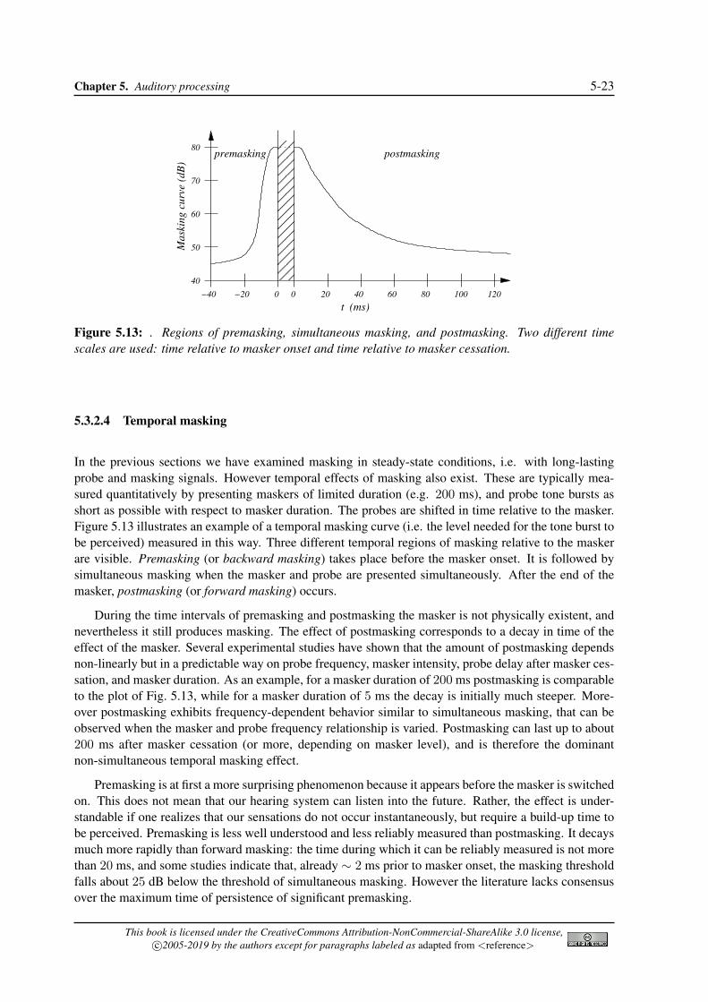
Figure 5.13: . Regions of premasking, simultaneous masking, and postmasking. Two different timescales are used: time relative to masker onset and time relative to masker cessation.
5.3.2.4 Temporal masking
In the previous sections we have examined masking in steady-state conditions, i.e. with long-lastingprobe and masking signals. However temporal effects of masking also exist. These are typically mea-sured quantitatively by presenting maskers of limited duration (e.g. 200 ms), and probe tone bursts asshort as possible with respect to masker duration. The probes are shifted in time relative to the masker.Figure 5.13 illustrates an example of a temporal masking curve (i.e. the level needed for the tone burst tobe perceived) measured in this way. Three different temporal regions of masking relative to the maskerare visible. Premasking (or backward masking) takes place before the masker onset. It is followed bysimultaneous masking when the masker and probe are presented simultaneously. After the end of themasker, postmasking (or forward masking) occurs.
During the time intervals of premasking and postmasking the masker is not physically existent, andnevertheless it still produces masking. The effect of postmasking corresponds to a decay in time of theeffect of the masker. Several experimental studies have shown that the amount of postmasking dependsnon-linearly but in a predictable way on probe frequency, masker intensity, probe delay after masker ces-sation, and masker duration. As an example, for a masker duration of 200 ms postmasking is comparableto the plot of Fig. 5.13, while for a masker duration of 5 ms the decay is initially much steeper. More-over postmasking exhibits frequency-dependent behavior similar to simultaneous masking, that can beobserved when the masker and probe frequency relationship is varied. Postmasking can last up to about200 ms after masker cessation (or more, depending on masker level), and is therefore the dominantnon-simultaneous temporal masking effect.
Premasking is at first a more surprising phenomenon because it appears before the masker is switchedon. This does not mean that our hearing system can listen into the future. Rather, the effect is under-standable if one realizes that our sensations do not occur instantaneously, but require a build-up time tobe perceived. Premasking is less well understood and less reliably measured than postmasking. It decaysmuch more rapidly than forward masking: the time during which it can be reliably measured is not morethan 20 ms, and some studies indicate that, already ∼ 2 ms prior to masker onset, the masking thresholdfalls about 25 dB below the threshold of simultaneous masking. However the literature lacks consensusover the maximum time of persistence of significant premasking.
This book is licensed under the CreativeCommons Attribution-NonCommercial-ShareAlike 3.0 license,c⃝2005-2019 by the authors except for paragraphs labeled as adapted from <reference>

5-24 Algorithms for Sound and Music Computing [v.February 2, 2019]
5.3.3 Auditory filters and critical bands
5.3.3.1 The power spectrum model of masking
Imagine the following experiment: the masking threshold for a sinusoidal probe is measured as a functionof the bandwidth of a band-pass noise masker, centered at the sinusoid frequency, and with constant leveldensity (so that the total noise level increases with the bandwidth). This experiment has been performedseveral times by many researchers, always yelding similar results: for small noise bandwith values, thethreshold increases with the noise bandwidth; however, above a certain bandwith value the thresholdflattens off and is not changed significantly by further increases in noise bandwidth.
A way of interpreting this result is the following: looking back at Fig. 5.4, we can model the behaviorof the basilar membrane as a bank of bandpass filters with overlapping passbands, the auditory filters.The probe is detected by looking at the output of the auditory filter centered on the probe frequency.Increases in noise bandwidth result in more noise passing through that filter, as long as the noise band-width is less than the filter bandwidth. However, once the noise bandwidth exceeds the filter bandwidth,further increases do not change the noise passing through that specific filter. The bandwidth at which thesignal threshold ceases to increase is called the critical bandwidth (CB), and it is closely related to thebandwidth of the auditory filter at the same center frequency.
This “band-widening” experiment is important because it leads to the so-called power-spectrummodel of masking, which assumes that (a) the peripheral auditory system behaves as a bank of over-lapping bandpass filters, (b) only one filter is used to detect a sinusoidal signal in a noise background(the one with center frequency corresponding to that of the signal), (c) the threshold for detecting thesignal is determined only by a certain signal-to-noise ratio at the output of that filter. Although noneof these assumptions is strictly correct (in particular, the filters are level dependent rather than linear,and listeners can combine information from more than one filter to enhance signal detection), the basicconcept of the auditory filter is widely accepted and has proven useful. The power-spectrum model ofmasking then predicts that simultaneous masking occurs when the the masker has energy in the samecritical band of the probe signal. In reality simultaneous masking effects are not bandlimited to withinthe boundaries of a single critical band. Interband masking also occurs, i.e., a masker centered withinone critical band has some predictable effect on the masking thresholds in other critical bands: this effectis known as the spread of masking.
Extensive research has been devoted to determining auditory filter shapes and the critical bandwidths.It is immediately evident that auditory filters do not have a rectangular magnitude response. In fact, ifthey were rectangular (with a bandwith exactly equal to the CB), then according to hypothesis (c) ofthe power-spectrum model the following equation would hold for the threshold level Lth of a sinusoidalprobe masked by broadband white noise with level density Lmask:
Lth = K · [CB · Lmask] , (5.13)
where CB · Lmask is the total masker level (because all noise components within the CB are passedequally and all components outside the CB are removed totally), and K is the signal-to-noise ratio atthreshold. According to Eq. (5.13), for subcritical bandwidths the signal threshold should increase by3 dB per doubling of bandwidth (i.e. 3 dB increase in masker level). Instead experimental data show thatthe rate of change is markedly less than this, thus providing evidence that auditory filters are not evenapproximately rectangular.
A first hint at the shape of the auditory filters is given by the so-called psychophysical tuning curves(PTC). In Sec. 5.3.2 we have used the four variables of masking experiments (probe and masker fre-quency and level) to plot masking curves, that represent the threshold level of the probe in the presenceof a masker of given level and frequency, as a function of probe frequency. We can use these variables in
This book is licensed under the CreativeCommons Attribution-NonCommercial-ShareAlike 3.0 license,c⃝2005-2019 by the authors except for paragraphs labeled as adapted from <reference>

Chapter 5. Auditory processing 5-25
102
103
104
0
20
40
60
80
100
f (Hz)
SP
L (
dB
)
Figure 5.14: Qualitative psychophysical tuning curves for six different probe signals (probe frequenciesand levels are indicated by circles), as a function of masker frequency.
a different way: namely, we can plot the masker level needed in order to mask a probe of given level andfrequency, as a function of the masker frequency. The curves that we obtain in this way are the PTCs.
The masker can be either a sinusoid or narrow-band noise, but noise is generally preferred to estimatePTCs, because it reduces beating effects. Moreover, low levels are generally used to ensure that activitywill be produced primarily in a single auditory filter. A qualitative example of PTCs is displayed inFig. 5.14. Two aspects are typical for these curves: the slope towards low frequencies is shallowerthan the slope towards higher frequencies, and the minimum is reached at a masker frequency a littlebit above the frequency of the probe. Note that these curves are in good agreement with physiologicaltuning curves discussed in Sec. 5.2.2.
According to the power-spectrum model, at threshold the masker produces a constant output from thecorresponding auditory filter, in order to mask the fixed probe. Thus the PTC indicates the masker levelrequired to produce a fixed output from the corresponding auditory filter, as a function of frequency. Ifwe mantain the assumption that the auditory filter are approximately linear with respect to masker level,we can conclude that the shape of the auditory filter can be obtained by inverting the PTC, because whatwe are doing is plotting the input required to give a fixed filter output.
5.3.3.2 Estimating the auditory filter shape
PTCs only give a qualitative idea of the shape of auditory filters, since they suffer from two main limita-tions. First, it is not strictly true that only one auditory filter is involved in the determination of a PTC,and instead “off-frequency” listening occur. Second, it is not strictly true that auditory filters are linearwith respect to masker level, so that the underlying filter shape changes as the masker is altered.
If we consider a generic non-rectangular magnitude response W (f) of the auditory filter, the follow-ing equation would hold for the threshold level Lth of a sinusoidal probe masked by broadband whitenoise with level density Lmask:
Lth = K
∫ +∞
0W (f)Lmask(f)df, (5.14)
where K is the signal-to-noise ratio at threshold, as in Eq. (5.13). Some experiments indicate that Kis typically about 0.4 and varies with center frequency, increasing markedly at low frequencies. Bymanipulating Lmask(f) and measuring the corresponding changes in Lth it is possible to infer the filter
This book is licensed under the CreativeCommons Attribution-NonCommercial-ShareAlike 3.0 license,c⃝2005-2019 by the authors except for paragraphs labeled as adapted from <reference>

5-26 Algorithms for Sound and Music Computing [v.February 2, 2019]
������������������������������
������������������������������
����������������������������������������
����������������������������������������
f0
f∆ f∆
Noise Noise
Auditory filter
f (Hz)
Probesignal
(a)
102
103
10
15
20
25
30
35
40
45
50
∆ f (Hz)
Maskin
g c
urv
e (
dB
)
(b)
Figure 5.15: Auditory filter estimation through a notched-noise experiment; (a) magnitude responsesof sinusoidal probe, notched-noise masker, and auditory filter; (b) measured masking threshold as afunction of notch half-bandwidth ∆f .
shape W (f). The masker used to perform measures should be such that the assumptions of the power-spectrum model are not strongly violated. An approach used in the literature is the “notched-noisemethod”, which employs a broadband white noise masker with a notch around the probe frequency f0.The filter shape can then be estimated by measuring the masking threshold as a function of the widthof the notch. Figure 5.15(a) illustrates a notched noise experiment, in which the notch is symmetricalaround f0 and has a width of 2∆f . In this case from Eq. (5.14) one can write
Lth = KLmask
∫ f0−∆f
0W (f)df +KLmask
∫ +∞
f0+∆fW (f)df. (5.15)
The two integrals on the right-hand side represent the shaded areas in Fig. 5.15(a). Assuming that thefilter is also symmetrical about f0 (which is not too wrong for low noise levels) the two areas are equal.Thus, the threshold function provides a measure of the integral of the auditory filter.
If one assumes an analytical form of the auditory filter shape, then the integrals in Eq. (5.15) can bealso solved analytically. Many investigators have used a family of such analytical forms, constructed asan exponential with a rounded top, and called roex for brevity. The simplest of these forms, the roex(p)filter, can be written as
W (g) = (1 + pg) · exp(−pg), with g = | f − f0 | /f0. (5.16)
The new variable g represents normalized frequency deviation from f0, while the parameter p determinesboth the bandwidth and the slope of the skirts of the auditory filter. The higher the value of p, themore sharply tuned is the filter. Moreover, asymmetric filter shapes can be described if two different pvalues pl, pu, are used independently for the lower and upper frequency filter skirts. Using roex models,Eq. (5.15) can be solved analytically and standard minimization procedures can be used to find the valuesof pl, pu that best fit experimental data.
5.3.3.3 Barks and ERBs
Using results from notched-noise masking experiments (or from other experiments that use differentapproaches) one can estimate the critical bandwidth as a function of frequency. Figure 5.15(b) providesa qualitative example of experimental data for f0 = 2 kHz Lmask = 50 dB. The masking threshold
This book is licensed under the CreativeCommons Attribution-NonCommercial-ShareAlike 3.0 license,c⃝2005-2019 by the authors except for paragraphs labeled as adapted from <reference>

Chapter 5. Auditory processing 5-27
101
102
103
104
102
103
f (Hz)
Bandw
idth
(H
z)
Critical bandwidth
ERB
(a)
0 0.5 1 1.5 2
x 104
0
5
10
15
20
25
f (Hz)
Critica
l b
an
d r
ate
(B
ark
)
CB filter frequencies
(b)
Figure 5.16: (a) Critical bandwidths, Eq. (5.17), and equivalent rectangular bandwidths, Eq. (5.19), asfunctions of center frequency; (b) the critical-band rate scale, Eq. (5.18), that maps Hz into Barks.
curve stays almost constant for small ∆f and decreases for ∆f larger than a critical value, which can beassumed as a measure of the critical bandwidth at 2 kHz.
By collecting data from many subjects an estimate of the critical bandwidth can be obtained. Ingeneral it is found that the CB remains almost constant (CB ∼ 100 Hz) up to a frequency of about500 Hz, increases slightly little less-than-linearly up to 3 kHz, and slightly more-than-linearly above3 kHz. This behavior can be reasonably approximated by assuming constant CB = 100 Hz up to500 Hz, and a CB increase of 20% of the center frequency above 500 Hz. For an average listener, CB isconveniently approximated as
CB(f) = 25 + 75 ·
[1 + 1.4
(f
1000
)2]0.69
. (5.17)
The plot of this function is shown in Fig. 5.16(a).Although the function is continuous, it is useful when building practical systems to treat the ear as
a discrete set of bandpass filters that conforms to Eq. (5.17). A particular filter set can be iterativelyconstructed as follows: given one filter, the next one is chosen in such a way that the upper limit of theCB of the current filter corresponds to the lower limit of the CB of the next one. This procedure leads tothe so-called scale of critical-band rate. The first CBs span the ranges [0, 100] Hz, [100, 200] Hz, etc.,up to 500 Hz where they start to increase. The critical-band rate function can be described as
z(f) = 13 · arctan (0.00076 · f) + 3.5 · arctan
[(f
7500
)2]
(Bark). (5.18)
Distance between critical bands along this scale is conventionally measured according to a new unit ofmeasure, called Bark: a distance of one CB is “one Bark”. The plot of the critical-band rate functionz(f) is shown in Fig. 5.16(b), while Table 5.1 provides values for a filter-bank based on the critical-bandrate. The corresponding numbered points in Fig. 5.16(b) illustrate that the nonuniform Hz spacing of thefilter bank is actually uniform on a Bark scale.
A characterization alternative to the critical-band rate and the Bark unit is the so-called ERB scale.The acronym ERB stands for Equivalent Rectangular Bandwitdth, and refers to a general way of char-acterizing the bandwidth of a bandpass filter W (f). The ERB of W (f) is defined as the bandwidthof a filter with rectangular magnitude response, constructed as follows: its center-frequency f0 is the
This book is licensed under the CreativeCommons Attribution-NonCommercial-ShareAlike 3.0 license,c⃝2005-2019 by the authors except for paragraphs labeled as adapted from <reference>
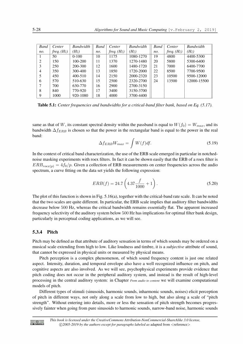
5-28 Algorithms for Sound and Music Computing [v.February 2, 2019]
Bandno.
Centerfreq. (Hz)
Bandwidth(Hz)
Bandno.
Centerfreq. (Hz)
Bandwidth(Hz)
Bandno.
Centerfreq. (Hz)
Bandwidth(Hz)
1 50 0-100 10 1175 1080-1270 19 4800 4400-53002 150 100-200 11 1370 1270-1480 20 5800 5300-64003 250 200-300 12 1600 1480-1720 21 7000 6400-77004 350 300-400 13 1850 1720-2000 22 8500 7700-95005 450 400-510 14 2150 2000-2320 23 10500 9500-120006 570 510-630 15 2500 2320-2700 24 13500 12000-155007 700 630-770 16 2900 2700-31508 840 770-920 17 3400 3150-37009 1000 920-1080 18 4000 3700-4400
Table 5.1: Center frequencies and bandwidths for a critical-band filter bank, based on Eq. (5.17).
same as that of W , its constant spectral density within the passband is equal to W (f0) = Wmax, and itsbandwidth ∆fERB is chosen so that the power in the rectangular band is equal to the power in the realband:
∆fERBWmax =
∫W (f)df. (5.19)
In the context of critical band characterization, the use of the ERB scale emerged in particular in notched-noise masking experiments with roex filters. In fact it can be shown easily that the ERB of a roex filter isERBroex(p) = 4f0/p. Given a collection of ERB measurements on center frequencies across the audiospectrum, a curve fitting on the data set yields the following expression:
ERB(f) = 24.7
(4.37
f
1000+ 1
). (5.20)
The plot of this function is shown in Fig. 5.16(a), together with the critical-band rate scale. It can be notedthat the two scales are quite different. In particular, the ERB scale implies that auditory filter bandwidthsdecrease below 500 Hz, whereas the critical bandwidth remains essentially flat. The apparent increasedfrequency selectivity of the auditory system below 500 Hz has implications for optimal filter bank design,particularly in perceptual coding applications, as we will see.
5.3.4 Pitch
Pitch may be defined as that attribute of auditory sensation in terms of which sounds may be ordered on amusical scale extending from high to low. Like loudness and timbre, it is a subjective attribute of sound,that cannot be expressed in physical units or measured by physical means.
Pitch perception is a complex phenomenon, of which sound frequency content is just one relatedaspect. Intensity, duration, and temporal envelope also have a well recognized influence on pitch, andcognitive aspects are also involved. As we will see, psychophysical experiments provide evidence thatpitch coding does not occur in the peripheral auditory system, and instead is the result of high-levelprocessing in the central auditory system: in Chapter From audio to content we will examine computationalmodels of pitch.
Different types of stimuli (sinusoids, harmonic sounds, inharmonic sounds, noises) elicit perceptionof pitch in different ways, not only along a scale from low to high, but also along a scale of “pitchstrength”. Without entering into details, more or less the sensation of pitch strength becomes progres-sively fainter when going from pure sinusoids to harmonic sounds, narrow-band noise, harmonic sounds
This book is licensed under the CreativeCommons Attribution-NonCommercial-ShareAlike 3.0 license,c⃝2005-2019 by the authors except for paragraphs labeled as adapted from <reference>

Chapter 5. Auditory processing 5-29
102
103
104
102
103
Reference frequency f1 (Hz)
Ha
lf p
itch
fre
qu
en
cy f
2 (
Hz)
102
103
104
102
103
Ra
tio
pitch
(m
el)
Half pitch
Ratio pitch0.5f
1
(a)
0 2000 4000 6000 8000 10000 12000 14000 160000
500
1000
1500
2000
2500
3000
3500
4000
Frequency (Hz)
Ratio p
itch (
mel)
Mel scale
Identity
(b)
Figure 5.17: Constructing the mel scale: (a) relation between frequency f1 of reference sinusoid andfrequency f2 of a comparison sinusoid producing half pitch sensation (solid curve), and absolute “ratiopitch” sensation as a function of frequency (the dashed line is the line f2 = 1.5 · f1); (b) absolute “ratiopitch” sensation as a function of frequency in linear scales.
with low harmonics missing, down to various types of noise. As an example, a sinusoid at 1 kHz pro-duces a very distinct strong pitch sensation, whereas a high-pass noise with a cut-off freq. of 1 kHzproduces an extremely faint pitch, although both stimuli produce approximately the same pitch sensationin terms of height.
5.3.4.1 Sinusoids and the mel scale
There are various procedures to measure the pitch of sinusoidal sounds with respect to their frequency.Typical methods are “halving (or doubling) procedures”, in which subjects are presented with a referencesinusoid at frequency f1 and have to adjust the frequency f2 of a comparison sinusoid until it is perceivedhalf (or twice) as high as the first one. At low frequencies (roughly, below 1−2 kHz), the halving of pitchsensation corresponds approximately to a ratio of 2 : 1 between sinusoid frequencies. This result is notsurprising, since in musical terms it corresponds to the octave interval. For higher values of f1, however,some unexpected results are found: a frequency ratio larger than 2 : 1 is necessary for the perception ofhalf pitch. This relation is illustrated in Fig. 5.17(a): the solid curve represents averaged data obtainedfrom half pitch and double pitch experiments (with the appropriate interchange of axes).
This curve is determined from experiments with halving and doubling of sensations rather than ab-solute values, by choosing an arbitrary pitch reference point. We can construct an absolute scale thatdefines the sensation “ratio pitch” as function of frequency. If we choose the reference point at low fre-quencies, where f1 and f2 are proportional, and assume that the constant of proportionality is 1, then wecan trace the dotted line in Fig. 5.17(a), by shifting the solid line by a factor of 2 towards the left. Thisdotted line indicates that at low frequencies values of ratio pitch are identical to values in Hz, while athigh frequencies values in Hz and values of ratio pitch deviate substantially from another.
The unit of this absolute ratio pitch sensation is called mel, since ratio pitch determined this wayis related to our sensation of melodies. As an example the dotted line in Fig. 5.17(a) shows that 8 kHzcorrespond to 2100 mel, while 1300 Hz correspond to 1050 mel, which confirms our previous observationthat a tone of 1300 Hz produces half the pitch of an 8 kHz tone. Figure 5.17(b) shows the same relation
This book is licensed under the CreativeCommons Attribution-NonCommercial-ShareAlike 3.0 license,c⃝2005-2019 by the authors except for paragraphs labeled as adapted from <reference>

5-30 Algorithms for Sound and Music Computing [v.February 2, 2019]
using linear scales. Possible parametrizations of the mel scale are the following:
m = 1127 · ln(1 +
f
700
), or m = 1000 · log2
(1 +
f
1000
), (5.21)
where the first one is the most commonly used. The similarity between the curve in Fig. 5.17(b) and theone in Fig. 5.16(b) suggests that there is a relationship between the mel scale and the critical-band scaleof Eq. (5.18). This is not so surprising if one assumes pitch to be determined by the center of excitationactivity along the basilar membrane, which is also reflected in the Bark scale.
As mentioned before, the pitch of sinusoids depends not only on frequency but also on other param-eters. Two particularly relevant factors are sound pressure level and partial masking. Psychophysicalexperiments show that pitch decreases with increasing sound pressure level for frequencies below 1 kHz,is quite independent on sound pressure level for frequencies in the range 1 − 2 kHz, and tends to risewith increasing sound pressure level for higher frequencies. As far as partial masking is concerned, itseffects on pitch can be roughly summarized as follow: a masker with a lower frequency content than theprobe yields positive probe pitch shifts, whereas a masker with a higher frequency content than the probeproduce negative pitch shifts. In terms of the corresponding excitation patterns, the pitch of the probe is“shifted away” from the spectral slope of the partial-masking sound.
A final important measure of pitch of pure sinusoids is the JND (just noticeable difference) betweenthe pitch of two sinusoidal sounds with different frequencies presented sequentially. There is somesmallest frequency difference below which listeners can no longer tell consistently which of the soundsis higher: the JND is usually defined as the frequency difference that produces 75% correct responsesin a “forced-choice” experiment. The pitch JND depends on frequency, intensity, and tone duration.Typically it is found to be about 1/30 of the critical bandwidth at the same frequency.
5.3.4.2 Harmonic sounds and pitch illusions
With respect to sinusoids, harmonic sounds produce a much less univocal pitch percept. The specificspectral characteristics of a harmonic sound can produce different results in terms of perceived pitch.
If the lowest harmonic component (the fundamental) is present, then the perceived pitch will usuallycorrespond to the frequency of this component, as one would expect. However if the fundamental ismissing and only higher harmonic components are present, the pitch perceived by a listener is still thatof this missing fundamental. A familiar example of the occurrence of such a virtual pitch phenomenonis that of a low pitched sound emitted by a very small loudspeaker (e.g., a voice emitted by the speakerof a laptop pc). Although such a loudspeaker radiates negligible power in the frequency range where thefundamental is located, listeners are still able to recognize the pitch.
The virtual pitch phenomenon does not always occur, only specific combinations of fundamentalfrequency and of the frequency of the lowest component are able to produce it. The existence region ofvirtual pitch can be defined as a close region in a cartesian plane whose axes are the lowest harmoniccomponent of the sound and the (missing) fundamental frequency. This region represents the area inwhich spectral components of incomplete harmonic spectra have to be contained in order to producea virtual pitch. Figure 5.18 shows a qualitative plot of such an existence region (detailed shapes varydepending on the stimulus type, in particular the number of harmonic components). This figure indicatesthat a harmonic sound with its lowest frequency component above 5 kHz will hardly produce any virtualpitch, whatever the missing fundamental frequency.
The missing fundamental phenomenon has been observed experimentally by many researchers sincethe 1840’s. The debate about its explanation has generated two alternative theories, one explaining thepitch sensation associated to the missing fundamental as a nonlinear difference tone generated at theauditory periphery, the second explaining the phenomenon as a result of processing operated by the
This book is licensed under the CreativeCommons Attribution-NonCommercial-ShareAlike 3.0 license,c⃝2005-2019 by the authors except for paragraphs labeled as adapted from <reference>

Chapter 5. Auditory processing 5-31
fund
amen
tal f
requ
ency
(H
z)
100 200 500 1000 2000 5000100
200
500
1000
frequency of lowest harmonic component (Hz)
Existen
ce re
gion
Figure 5.18: Qualitative plot of the existence region for virtual pitch.
central auditory system (with no involvement of the peripheral system). In particular some experimentshave shown that two successive harmonic partials (say with frequencies f1 = nf0 and f2 = (n +1)f0, where f0 is the missing fundamental), presented simultaneously to different ears, evoke an equallyeffective fundamental pitch percept as a monaural presentation of the same two harmonics. Clearly, ifeach of the two harmonic partials is delivered to a different ear, there can not be any physical interferenceat the level of the basilar membrane. This kind of experiments then suggest that the pitch of complextones is mediated primarily by a central mechanism that operates on neural signals derived from thosestimulus harmonics spectrally resolved in the cochlea.
Another well known auditory illusion in the perception of pitch is the so-called phenomenon ofcircular pitch. The illusion is generated by constructing a harmonic sound made of sinusoidal compo-nents with equal amplitudes and frequencies fk separated by octave intervals (i.e. f2 = 2f1, . . . fk =2kf1, . . .). This harmonic spectrum is passed through a filter with a fixed, band-pass shaped amplituderesponse (e.g. a cosinusoidal or a gaussian shape). Then the frequencies fk are shifted upwards ordownwards, either in discrete steps of a musical semitone, or in a continuous fashion.4 The perceptualresult is that of a scale or a tone which possesses a continually ascending (or descending) pitch, and yetultimately seems to go no higher or lower, i.e. it possesses a circular pitch. This is often regarded asa kind of auditory analog to visual effects where 2-D perspectives can create illusions of “impossible”geometries.5
5.3.4.3 Inharmonic sounds
Pitch perception of inharmonic sounds has also been studied. Consider a harmonic sound having strongpartials with frequencies of 800, 1000, and 1200 Hz. This will have a virtual pitch corresponding tothe missing fundamental at 200 Hz. If each of these partials is shifted upward by a small amount ofHz, however, they are no longer in exact harmonic relationship and do not have a common fundamentalfrequency. However listeners will typically still interpret this sound as being “nearly harmonic”, and willidentify a virtual pitch of approximately 204 Hz. This pitch sensation can be interpreted as a result oflooking for a “nearly common factor”: 1/[(820/4) + (1020/5) + (1220/6)] ∼ 204.
4In the former case, the resulting sound is known as the Shepard scale, in the latter it is known as the Risset tone.5Some famous and striking examples of impossible perspectives, like ever-ascending stairs, can be found in the work of
dutch graphic artist M. C. Escher.
This book is licensed under the CreativeCommons Attribution-NonCommercial-ShareAlike 3.0 license,c⃝2005-2019 by the authors except for paragraphs labeled as adapted from <reference>

5-32 Algorithms for Sound and Music Computing [v.February 2, 2019]
5.4 Commented bibliography
Review of distal, medial, proximal theories by Bullot et al. [2004].General reference in psychoacoustics. Classic book by Fastl and Zwicker [2007]. Also check Moore
[1995]. Georg von Bekesy, the Nobel laureate, was one of first to study the inner ear and the cochlea.His pioneering observations established concepts of the traveling wave and the CF for different placesalong the cochlea. He described his observations in [von Bekesy, 1960].
Physiology and mechanics of the inner ear and cochlea: review paper by Robles and Ruggero [2001],with a strong focus on experimental measurements. Another review paper on the cochlea, more focusedon the cochlear amplifier and modeling approaches, is [Nobili et al., 1998]. The cochlear model reportedin Eqs. (5.3-5.7) is based on this paper.
Loudness and equal-loudness contours: a recent and interesting review of the topic is provided bySuzuki and Takeshima [2004], which has led to the revision of the ISO226 standard. Our fig. 5.8(b) isbased on the data contained in this work.
Perceptual coding: an extensive review is provided by Painter and Spanias [2000].
ReferencesNicolas Bullot, Roberto Casati, Jerome Dokic, and Maurizio Giri. Sounding objects. In Proc. Int. Workshop “Les journes du
design sonore”, Paris, Oct. 2004.
Hugo Fastl and Eberhard Zwicker. Psychoacoustics. Facts and models. Springer-Verlag, Heidelberg, 3rd edition, 2007.
Brian C. J. Moore, editor. Hearing – Handbook of Perception and Cognition. Academic Press, San Diego, 2nd edition, 1995.
Renato Nobili, Fabio Mammano, and Jonathan F. Ashmore. How well do we understand the cochlea? Trends in Neurosciences,21(4):159–167, Apr. 1998.
Ted Painter and Andreas Spanias. Perceptual coding of digital audio. Proceedings of the IEEE, 88(4):451–515, Apr. 2000.
Luis Robles and Mario A. Ruggero. Mechanics of the mammalian cochlea. Physiol. Rev., 81(3):1305–1352, July 2001.
Yoiti Suzuki and Hisashi Takeshima. Equal-loudness-level contours for pure tones. J. Acoust. Soc. Am., 116(2):918–933, Aug.2004.
Georg von Bekesy. Experiments in hearing. McGraw-Hill, New York, 1960.
This book is licensed under the CreativeCommons Attribution-NonCommercial-ShareAlike 3.0 license,c⃝2005-2019 by the authors except for paragraphs labeled as adapted from <reference>

Contents
5 Auditory processing 5-15.1 Introduction . . . . . . . . . . . . . . . . . . . . . . . . . . . . . . . . . . . . . . . . . 5-15.2 Anatomy and physiology of peripheral hearing . . . . . . . . . . . . . . . . . . . . . . 5-2
5.2.1 Sound processing in the middle and inner ear . . . . . . . . . . . . . . . . . . . 5-25.2.1.1 The middle ear . . . . . . . . . . . . . . . . . . . . . . . . . . . . . . 5-25.2.1.2 The cochlea and the basilar membrane . . . . . . . . . . . . . . . . . 5-35.2.1.3 Spectral analysis in the basilar membrane . . . . . . . . . . . . . . . . 5-45.2.1.4 Cochlear traveling waves . . . . . . . . . . . . . . . . . . . . . . . . 5-65.2.1.5 The organ of Corti and the haircells . . . . . . . . . . . . . . . . . . . 5-6
5.2.2 Non-linearities in the basilar membrane . . . . . . . . . . . . . . . . . . . . . . 5-85.2.2.1 Input-output functions and sensitivity . . . . . . . . . . . . . . . . . . 5-85.2.2.2 Tuning curves and frequency selectivity . . . . . . . . . . . . . . . . 5-95.2.2.3 Two-tone interactions . . . . . . . . . . . . . . . . . . . . . . . . . . 5-10
5.2.3 Active amplification in the cochlea . . . . . . . . . . . . . . . . . . . . . . . . . 5-115.2.3.1 Experimental evidence for cochlear amplification . . . . . . . . . . . 5-115.2.3.2 Reverse transduction and OHC electromotility . . . . . . . . . . . . . 5-125.2.3.3 The cochlear amplifier at work . . . . . . . . . . . . . . . . . . . . . 5-13
5.3 Elements of psychoacoustics . . . . . . . . . . . . . . . . . . . . . . . . . . . . . . . . 5-155.3.1 Loudness . . . . . . . . . . . . . . . . . . . . . . . . . . . . . . . . . . . . . . 5-15
5.3.1.1 Threshold in quiet . . . . . . . . . . . . . . . . . . . . . . . . . . . . 5-155.3.1.2 Equal loudness contours and loudness scales . . . . . . . . . . . . . . 5-165.3.1.3 Weighting curves . . . . . . . . . . . . . . . . . . . . . . . . . . . . 5-18
5.3.2 Masking . . . . . . . . . . . . . . . . . . . . . . . . . . . . . . . . . . . . . . 5-195.3.2.1 Simultaneous masking: noise-masking-tone . . . . . . . . . . . . . . 5-205.3.2.2 Simultaneous masking: tone-masking-noise . . . . . . . . . . . . . . 5-225.3.2.3 Simultaneous masking: tone-masking-tone . . . . . . . . . . . . . . . 5-225.3.2.4 Temporal masking . . . . . . . . . . . . . . . . . . . . . . . . . . . . 5-23
5.3.3 Auditory filters and critical bands . . . . . . . . . . . . . . . . . . . . . . . . . 5-245.3.3.1 The power spectrum model of masking . . . . . . . . . . . . . . . . . 5-245.3.3.2 Estimating the auditory filter shape . . . . . . . . . . . . . . . . . . . 5-255.3.3.3 Barks and ERBs . . . . . . . . . . . . . . . . . . . . . . . . . . . . . 5-26
5.3.4 Pitch . . . . . . . . . . . . . . . . . . . . . . . . . . . . . . . . . . . . . . . . 5-285.3.4.1 Sinusoids and the mel scale . . . . . . . . . . . . . . . . . . . . . . . 5-295.3.4.2 Harmonic sounds and pitch illusions . . . . . . . . . . . . . . . . . . 5-305.3.4.3 Inharmonic sounds . . . . . . . . . . . . . . . . . . . . . . . . . . . . 5-31
5.4 Commented bibliography . . . . . . . . . . . . . . . . . . . . . . . . . . . . . . . . . . 5-32
5-33