A THEORY OP PINANCIAI. ANALYSIS, APPLYING

NON-LINEAH VARIABLES

by

SAM R. HUNTER, B.S. in E.E.

A THESIS

. IN

FINANCE

Submitted to the Graduate Faculty of Texas Technological College

in Partial Fulfillment of the Requirements for

the Degree of

MASTER OP BUSINESS ADMINISTRATION

Approved

Accepted

August, 1968

i í W f

-T Z<

,A;V '^0 TABLE OF COîîTEHTS

-'^' I . OBJECTIVE 1

Introduction , . . , . . . , . . , . . . . . 1

Statement of the Problem . . . . . . . . . . 1

Objective . . . . . , ' . " 3

Prooedure . . . . . . . . . . . . . . . . . 5

II, HISTORY OF INVESTI4ENT THSORY 7

Introductlon . , . . . • . , 7

The Linear Stock Model . . . . . . . . . . . 8

Implications of the Linear Stock Model . . . l^

The Non-Linear Stock Model 18

The Problem of Increasing Discount Rate . , 22

Theory Linking Investment and Stock Prlce , 22

III. TEE DISCOUNT FACTOR . , , . , , , , . . . . .' . 25

Introduction . . . . , . , , , , . , , , . , 25

Deflnition of the Discount Factor . . . . . 25

Components of the Discount Factor . . . . . 25

Assigning a Valiie to the Discount Factor , . 26

Conclusion , , . . , . . , , . . , . . . , . 29

IV. THE MODSL ' . 31

Ob^ective . , , , . . . . . . 3I

Economic Theory of the Model 3I

Gompertz Curve , , . , . . . . . , . , . . , 33

Implications of the Earnings Curye , . . , . 37

ii

iii

Grovjth Rates in Assets and Earnings . . . . . 38

Investment Rate ^O

Assets . , , , , , , , . . . . . ^^

Dividends and Stock Valuation . . . . ; . . . ^6

Conclusion , , . . . " , . . ^9

V. SUI^^ARY AND CONCLUSIONS 52

Summary . . . . . . . . . . . . . . . . . . . ' 52

Application' of the Gompertz Curve . . .,• . . . 5^

Application of the Model . . . . . , , , , . 55

Iraplications of the Model . . , , , . . . , . 5^

Conclusions . , . . , , , , . , , , , . ' . , . 59

BIBLIOGRAPHY 6

CHAPTER I

OBJECTIVE

ntroduction

The art of financial analysis is evolving today into

the science of financial analysis. The tools of scientifio

research and specialized procedures are being used to pene-

trate the aura of the financial world. Sub^jéctive procedures

of the past are being refined to create more objective ap-

praisals of the present. The research carried on and re-

ported in the past few years reflects this evolution.

In the past decade the emphasis of financial analys s

development has been towards the greater usê of analytical

models. The complete financial model tries to represent

mathematically the actions of the firm and the value that

the market places.. on these actions. Although the representa-

tion may be at variance to some extent with the financial

accoimts of a particular firm, the objective model does give

a clear picture of the interactions and reactions that take

p ace within its framework. As more mode s are developed

the characteristics of the many variables in financial analy-

sis aré better understood.

Statement of the Problem

In the thcory of the value of the firm, there are two

primary problems; (l) the estimate of dividends the firm

will pay, and (2) the determination of the value of the dis-

count factor that should be used to determine the present

worth of the firm's investment. If these values are knoTm,

the present price of the stock can be valuated. An integral

part of the problem is the coincident determination of the

earnings and assets of the firm. These financial factors are

a vital part of the determination of the dividends. A mathe-

ma,tical model encompassing these financial factors of invest-

ment is the sub;ject of this paper.

For the most part the models developed over the past

decade have concentrated on one particular part of the fi-

nanciaí activities of the firm. Although these models con-

tribute to the understanding, they are not extensive enough

to give a complete picture of the firm's financial activltles.

One particular model, the linear stock model, has been thor-

ough investigated. However, the basic assumptions of the

model make its outcome untenable, This model cannot func-

tion in the world of reality.

At the present time, there is no. mathematical model

that can accurately depict the financial activities of the

firm. The development of a model that encompasses these

activities would enhance the discipline of financial analy-

sis, Variables could be studied to ascertain their re-

actions and interactions. The model could be used to plan

the financial needs of the firm and to maximize the financlal

benefits. ín addition the investor could use the model in

determining his investments, The model could give the in-

vestor a more acciurate determination of the worth of the

investments available to him,

Ob.lective

This study will develop a general theory and financial

model depicting the earnings of the firm, From the earnings

of the firm, the values for dividends, assets, and stock

price will be developed and equated to earnings through the

various financial factors, The study dwells on.the theory

of the financial model and not on empirical findings from

its application,

The development of the earnings curve of a firm is based

on the Economic Lavj of Variable Proportions and the Gompertz .

Curve of Statistics. The Law of Variable Proportions is

also known as the Law of Diminishing Returns and is a "con-

cept laden with enormous consequences," The law assumes •

that economic conditions remain the same and that a factor

of production is increased unit by unit, As this factor is

Increased at first, the returns may be small, Further In-

crease brings more and more increase in returns per unit of

the production factor added, At a later stage the increase

M,- M. Bober, Intermediate Price and Income Theory. (rev.' ed. í New York: W. W. Norton & Com'pany, Inc. , 1955), PP. 103-121.

per unit of production factor begins to decline, but absolute

growth is still increasing. The rate of growth continues to

decline as more units of the production factor are added,

until it is uneconomical to add more units. We are assuming

that the rational firm will not add the production factor

past the economical point.

In this paper, the economical point is defined as the

point where an increase in a production factor does not yield

the return that the firm's investors require .on their invest-

ment. At this point, the growth rate approaches zero and the

retuxns approach a static level.

The Law of Variable Proportions is applied in this study

to the assets and earnings of the firm. The assets of the

firm, or scale of plant, is a factor of production, and the

earnings of the firm are the measure of the returns to this

factor.

The Gompertz growth rate curve is consistent with this

law and thus can provide a measure of the projected earnings.

With data from the firm the use of the science of statistics

can g ve a projection of the earnings of the firm and the

static upper level the earnings will approach. V/ith this

earnings projection, the future assets of the firm will be

related to earnings through the rate of return and the in-

vestment rate. Dividends will also be related to pro;3ected

earnings through the investment rate, The stock price is

the discounted value of the futnre dividends.

Procedure

The procedure used in this report vrill be first to

examine the published theories relating to the financial

activities of the firm dealing with assets, earnings, divi-

dends, and stock valuation. These theories are pre&ented .

in Chapter II and will be used as a base for the development

of this study. In Chapter II the theory related to the

linear stock model vrill be presented first. Reasoning will

then be developed showing why this theory is not valid. A

presenta,tioh wiil then be made on reasoning and published

opinions supporting a non-linear financial model. The chap-

ter will be concluded vrith a report on theory linking the

investment rate and the return that investors require.

Since the discount factor, k, is such an important part

of any financial model, a separate section is devoted to this

function. ' .In Chapter III past theories of the valuation of

k as well as theories of the author are presented. These

theories will provide direction in determining the value

•of k.

The model will then be presented with earnlngs as the

base in Chapter IV, Values for dividends, assets, and stock

valuation vjill be linked to the earnings curve. Along with

the model, guidelines will be presented to evaluate the earn-

ings curve and the factors that interrelate the other finan-

cial variables.

A summary of the application of the model and its use-

fulness will terminate the study in Chapter V,

CHAPTER II

HISTORY OF INVESTMENT THEORY

Introduction

Investigations in the theory of the value of the firm

have concentrated on two of the main aspects of investment:

the projected payments resulting from the investment, and

the value of the discount factor that should be used to yield

the present worth of the firm's stock. The projected pay-

ments are the primary aspect of the problem.

In this chapter, the vjork that has been done on the

theory will be shovjn from several different viewpoints. It

shall be established, by weight of authority and by logical

reasoning, that the present value of a security is the dis-

counted value of all future dividend payments. It shall also

be shown that there have been theoriesbased on either one

•or the other of two primary assumptions on the grovith of

dividends by writers.in the field. One assumption is that

dividends are grovring at a constant rate per year. This

assumption has been given the most attention. The other

assumption is that the dividends will grovj.but at some point

the growth will start declining and tend to level off. Evi-

dence will be given supporting both of these assumptions.

Hovjever, the author shall attempt to show that the constant

growth rate assumption is not valid.

8

A report on vjork that has been done linking investment

and stock price wil be given. Although thls work does not

give definite answers, it does give a criteria for investment

in theoretical terms.

The Llnear Stock Model

John B. Williams vjas a pioneer in the field of invest-

ment theory. His book, The Theory of Investment Value. pub-

lished in 1938, has been a guide for most of the writing in

the field. In the book, Williams investigated all the facets

on which today's theory is based.

Williams investigated the two primary areas of dividend

growth theory: (l) the assumption that the dividends of a

firm will have grovjth at a constant rate for an infinlte time

period and (2) the assumption that the nevj successful firm

will grow, but that at some point in time, the grovjth will

start decreasing and tend to level off.

In his book, Williams developed the follovring linear

stock valuation equation on the assmption that dividends

are growing at a constant rate per year:

Vo = TTo w lím (l-vj" ) ^ /2. 7 1 - w t—^OO -

where Vo = present worth of stock 'H'o = present dividends

. w = uv u = 1 + g, where g = growth .V = 1 , where i = discount factor

1+i

^John B. Williams, The Theory of Investment Value (Cam-bridge, Mass.: Harvard University Press, 1938), pp. 87-89, 128-135.

9

In the equation vj has to be less than one or the term

(1-w ) will not approach zero as t approaches infinity.

For w to be less than one, g must be less than i, As t goes

to infinity the resulting equation is:

Vo = Jl2-iî /2:27 1-w - —

Williams regarded this equation as strictly hypotheti-3

cal- and only an exercise in mathematics, The equation is

based on constãnt growth of dividends of the firm at the

rate g to infinity, In the words of Wall Street, "no tree

grows to the sky," which means that no firm has infinite

growth. Therefore, the equation is not valid.

The linear stock model, equation /^.27, has strong ap-

peal since some firms have exhibited a stable growth trend

over a long period of years. Investigations of the model

have been made from several different viewpoints. Since the

equation is linear and simple, it vjould be very important

to the financial world if a strong relation between reality

and the model could be established. Several articles and

books have been written with this equation as the base.

In 195^» John C. Clendenin and Maurice Van Cleeve re-

ported on a study of the characteristics of several mature

"growth" stocks. The range of grovjth rates of these stocks

^Tbid., pp. 89-9 1-.

John C. Clendenin and Maurice Van Cleeve, "Growth and Common Stock Values," The Journal of Finance. IX (195^), pp, 365-76, : [

10

for a 25 year period was 2% to 8^ per year. The presenta-

tion was made in k steps: (l) The authors illustrated the

price earnings ratios and yields prevailing in April, 195^,

on grovjth and non-growth stocks, and gave some examples of

price appreciation between 19^0 and 195 1- in such stocks. .

(2) They reaffirmed and commented on some aspects of the

theory that market prices of stocks should be re ated to the

discounted values of probable future dividends to be paid by

the firm. (3) They developed evidence on the rate of "growth"

which had been attained during the past 25 years by major

established corporations. (k) They presented tables which

indicated the computed values of stocks at reasonable dis-

count rates. These firms were assumed to pay dividends at

increasing rates in future years.

Messers, Clendenin and Van Cleeve presented a thorough

report on the past performance of these stocks and-presented

tables on hypothetical situations of the future concerning

grovjth rates and discount rates," Their grovjth rates were in

ranges of 5% dovm and with discount rates in the area of 5%-

This discount rate reflected the low. interest rates prevalent

during the period. One of the major conclusions of Clendenin

and Van Cleeve was that real grovjth in mature major corpora-

tions rare y exceeds 5% per annum.

In'this report, Clendenin and Van Cleeve established the

fact that large, mature corporations ezhibit a stable but

11

modest growth trend over a large number of years. This arti-

cle has been quoted by many of the authors vjho support the

linear stock model,

The authors suggested also in their presentation, that

remoté dividends or payments should be discounted at higher

values than near term payraents because of possible contin-

géncies or the decreasing marginal utility of the very re-

mote dividends,

David Durand discussed the linear model in his paper, . •

"Growth Stocks and the Petersburg Paradox,"-^ His research

for the paper led him to the classic vjork on probability by

Daniel Bernoulli in 1738, Bernoulli's paper pertains to an

exponentially grovjing series. Durand modifies the assump-

tions of Bernoulli's paper to apply to a grovjth stock. The

equation for valuation is developed as follovís: Po ='• D ^ -l- D (1-t-g) + D(l±g)^ +. — - D (1+g)^"^ ^ ^

T +TT (1+i) (l+i/2 (l+i)n /2,27 where Po = computed price of the security

D = dividends at the end of the first time period g'= constant grovith rate i = discount rate

- David Durand, "Growth Stocks and the Petersburg Para-dox," The Journal of Finance, Vol. XII (September, 1957), pp. ^k'E:^.

Daniel Bernoulli, "Exposition of a Nevj Theory on the Measurement of Risk," Economitrica. XXII (195^), 23-26, which is a translation by Dr. Louis Sommer of Bernoulli's paper, Speciamen Theorlcal Noval de Mensura Sortis. Com,Tnentarii Aca demiae Scientiarujn Imperialis Petropolitanae, V (1738^ PP, 175-92.

12

This series is arithmetically equivalent to a discounted series of dividend payments, grovjing at a constant rate, g, and discounted at rate i. The summation of the seri^s is a simple exercise in actuarial mathematics. The sum of the n terms is:

•±mÊ Po

i-S Z2.it7

provided i is different from gj the sum of an in-finite or very large nimber of terms approaches the very simple formulated quanity

7

provided that i exceeds g.

Diirand pointed out that the grovjth rate cannot equal or

exceed the discount rate in the above equation because the

evaluated price of the stock will then be equal to an infi-

nite or a negative price. Durand did not believe that the

linear stock model could be used to valuate stock in the o

world pf reality,

Myron J, Gordpn, realizing the limitations of the linear

stock model, used the model to develop and establish many

important characteristics of the firm, linking investment,

d^bt, taxes, and earnings,^ His arguments helped establish

that the expected dividends of the corporation is the primary

" Durand, "Grovjth Stocks," PP, 351-52,

^lbid., pp. 35^-60. o ' Myron J.'Gordon, The Investment. Financing. and Valua-

tion on the Corporation (Homewood, 111.; Richard D. Irwin, 'lnc, 1962).

13

determinate in stock evaluation. Equations for the inclusion

of debt and taxes in the financial activities pf the firm

were brought forth in this book. These equations establish

mathematical links in the chain of theory,

Even though Gordon based the discount factor pn the

grovjth rate of the firm in order to avoid the lack of real-

ism of the linear model, he showed the way in establishing

different functions of the discount factpr. Gordon split

up the discount factor into different functions and analyzed

them, The characteristics established have been used as a

base for other books and this paper.

Messers. Lerner and Carleton also expanded on the linear

stock model, Their methods in attacking the problem were

much more flexible, mathematically. The authors established

different mathematica relationships between the accounting

variables of the firm. Through ob;)ective mathematics, the

authors pioneered the vjay in showing how the different vari-

ab es of the firm can be used to-maximize the stock price.

These authors have shovjn that higher mathematics is the way

of the future for the financial analyst, Their analysis of

the firm is another building block of the financial analyst's

discipline.

Eugene M..Lerner and W. T, Carleton, A Theory of Financial Analysis (New York: Harcourt, Brace & World, Inc., T9SST7~

14

Implication of the Linear Stock Model

The linear stock model

Po = ^

where Po = present worth of stook D = dividends in the next time period k = discount factor g = grovjth, oonstant rate

vias examined by Gordon and Lerner and Carleton for applica-

tion to large mature corporations based on the premise that

grovjth is slovj and fairly stable. The primary assumption

of the linear model, that the firm vjould have infinite growth,

is untenable. Hovrever, it was felt that the far distant

future would have little or'no effect on the computed value

of the stock. With the infinite growth assumption of the

linear model, the computed value of the stock increases at an

increasing rate as g increases from zero.

A plot of k-g

with respect to g is shown in Figure 1.

1 k-g

0 '4M Vi^ %k k |'4K /î£k |3 2i<

g

Figure 1.

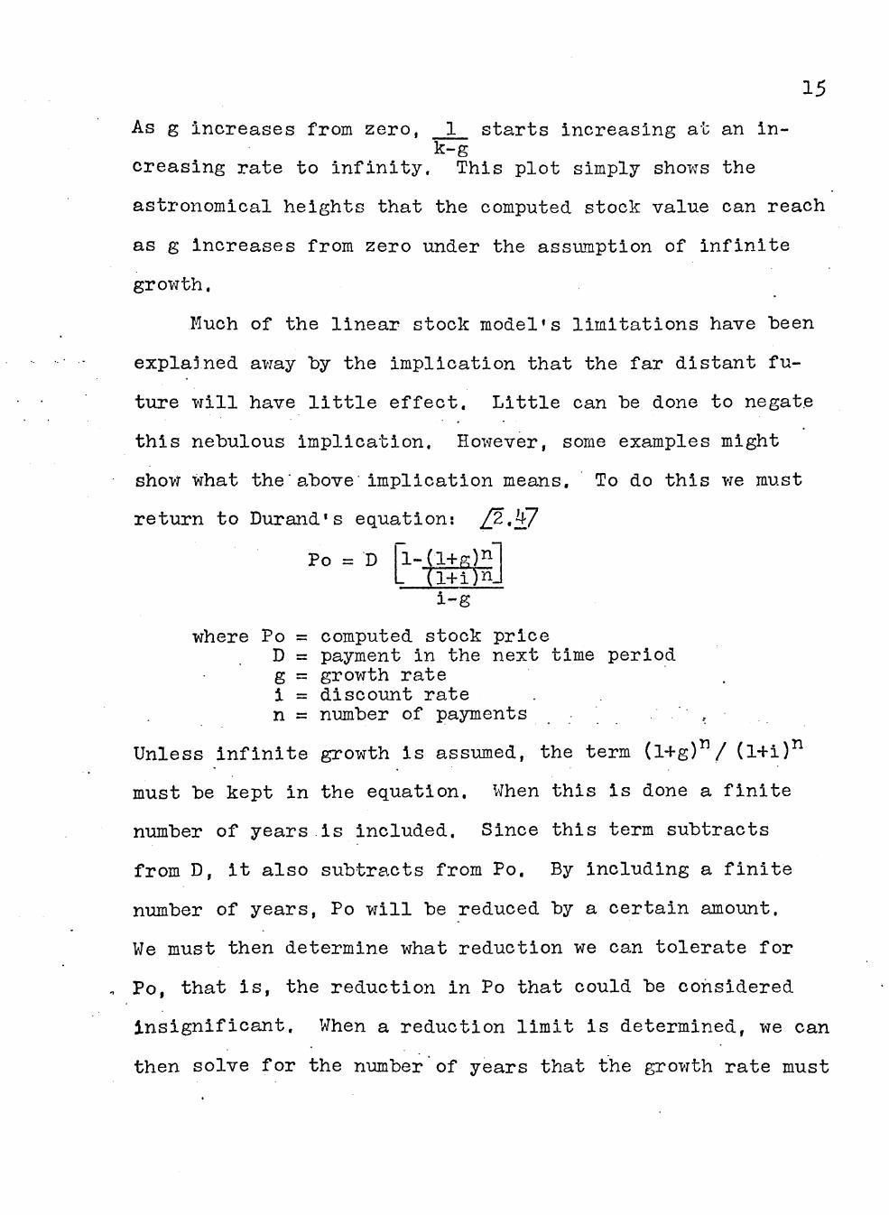
15

As g Increases from zero, 1 starts increasing at an in-k-g

creasing rate to infinity. This plot simply shovjs the

astronomical heights that the computed stock value can reach

as g increases from zero under the assumption of infinite

growth.

Much of the linear stock model's limitations have been

explained avjay by the implication that the far distant fu-

ture will have little effect. Little can be done to negate

this nebulous implication. However, some examples might

shovr what the'above implication means, To do this vje must

return to Durand's equation: /2.^7

Po = D fl-Cl+g)^ L (l+i)n_

i-g

where Po = computed stock price D = payment in the next time period g = growth rate i = discount rate n = number of payments . ,

Unless infinite growth is assumed, the term (l+g)"/ (l+i)^

must be kept in the equation. When this is done a finite

number of years.is included. Since this term subtracts

from D, it also subtracts from Po, By including a finité

number of years, Po will be reduced by a certain amount.

We must then determine what reduction we can tolerate for

Po, that is, the reduction in Po that could be considered

insignificant. When a reduction limit is determined, we can

then solve for the number of years that the grovjth rate must

16

continue in order to reach the reduced value of Po. Can a

lO^ reduction be tolerated, a 5^ or a \% reduction? For

example, assume a toleration limit of 5% reduction in the

numerator term only, then vihen

i = 7^

g = 0

and j ±||^ =.05, n ^ kk years.

The dividend must remain constant for approximately kh years

for the numerator terms of equation /2.^7 to reach 95^ of its

value under the infinite growth asswjiption,

When i = 7^

g = 2^

(1+P:)^ = .05, n = 130 years (l+i)n

The dividends must increase at a cônstant rate of 2%, for

130 years for the term to reach 95^ pf its value •under the

infinite grovjth assumption,

When i = 7^

g = 5%

(1+g)^ = .05, n = 330 years (1+i)^

The dividends must increase at a constant rate of 5% for

330 years to reach 95% of the numerator term tmder the in-

finite growth assumption. Also this rate of growth for 33O

years would require the dividends to increase 100,000,000

times their present size.

17

This demonstration indicates that any reasonable value

of g will show unrealistic values of stock price. Of course,

this is a judgment situation. The facts are presented to

the reader and the ^udgment is left to him.

Another possibility on this model was to make the dis-

count factor, k, a function of grovjth, The reasoning vjas

thát if the discount factor increased with the growth rate,

then the growth rate would not approach the discount factor.

But the discount factor is defined as the rate of return that

11 investors require, therefore, this assumption is untenable.

The discount factor is independent of groT-jth but is dependent

on a rate of interest and the uncertainty of the investor.

In defining the use of the discount factor, Williams said,

12 "Each investor should use his personal rate of interest."

If the investor is certain in his mind that the dividends

are predictable, the risk cpmponent in k is réduce.d and k

approaches the pure rate of interest.

The author believes.the arguments for the linear stock

model lead to unrealistic approaches to stock valuation. A

stock model using non-linear proportions would seem to be the

answer to the dilemma.

11 Lerner and Carleton, Financial Analysis, p. 108.

• Williams," Investment Value. p. 59. •

18

The Non-linear Stock Model

Williams realized the implications of a stock model

that exhibited infinite growth. He suggested that most suc-

cessful firms will exhibit fast growth in the early stages

of their development. Later the firm's growth rate will.

start declining, but absolute growth will continue. The

general curve for this reasoning is shovm in the Figure 2.

Dividends

Figure 2

For purposes of illústration, V/illiams divided the life

cycle of the firm into three parts as shovm in Figure .2.

The three stages are (l) the early period when growth is

fast, (2) the period when the growth rate begins to decline

markedly, and (3) the period when the firm is mature, when

growth is slow and is asymptotic to a maximum level. He then

assumed, as a special case, that the asymptote was equal to

twice the dividend at the end of the first stage, i.e., at

n in Figure 2 above.

19

With these assumptions he developed the equation: -

Vo = TT o w /2.27

using the same notations as in equation /2,27. This equation

was an exercise to show how a curve of this order mi-ght be

attacked. His assumption limited the formula to a curve that

would describe the actions as stated above. It was not in-

tended to be a general formula,

In referring to the curve, Williams said, "Any other

function that lends itself to convenient mathematical treat-

men't may be used, so long as the general premise that the

stocks derive their value from their future dividends is

l^ adhered to."-

Mr, Williains derived other equations for special cases

of the curve, as he did in equation /2.27, yet he exhibited

no generaí .equation that vjould f it tho; curve. Estlmates of •

length of growth could be made on Judgment and substituted

in the special cases he exhibited. Hovjever, the reliability

of the estimate would depend on the judgement of the estima-

tor rather than a scientific evaluation.

The full impact of V/illiam's work has not been felt by

the financial analyst. The mathematics in his book was

-^Williams, Investment Value. p. 9 . Ik • - -

Ibid.. p. 9 .

20

complicatedj therefore, it did not achieve popular acclaim.

Williams was a man ahead of his time.

Articles by James E. Walter and Charles C. Holt support

the non-linear model as described by Williams. These arti-

cles present the case from different viewpoints.

In an article published in 1956, James E. Walter classi-

fied stocks in three categories; (l) grovjth stock, (2) in-

termediate stocks, and (3) creditor stocks. - He classified

growth stocks as having a high rate of return with corre-

spondingly low dividend payout ratios. Intermediate stocks

were classified by medium to high dividend payout ratios

with average growth. Creditor stocks were classified by

high dividend payout ra tios and very modest grovjth. Walter's

classification of stock is con^istent with V/illiams' growth

rate curve, It was his opinion that stock prices, over long

periods of time reflect the present value of anticipated

future dividends. Walter pointed out that the stock price

difference is due to different dividend payout ratios be-

tween firms in both intermediate and creditor stock groups.

The higher dividend payout ratios resulted in hig"her stock

prices for firms in these groups, ceterius paribus.

Charles C. Holt compared present stock prices with

l^ • Jaraes E. Walter, "Dividend Policies and Common Stock Prices," The Journal of Pinance. Vol. XI (March, 1956) pp. 29-^1.•

21

projected duration of growth to investigate what the length

of grovjth would have to be to justify the present price,

His basic premise was that the earnings of grovrth vjould con-

tinue for some period of time but then would slow dovjn to

the rate that is normally achieved by mature companies in

general. He explained, "We hardly expect the growth of earn-

ings to terminate sharply but, rather, would expect the

growth rate to decline gradually as the special advantages .

enjoyed by the growth compahy are whittled away by increasing

competition, expiration of patents, appearance of substitute

17 products, etc." He stipulated that both the duration and

the rate of growth need to be taken into account in valuing

the growth stock.

Durand also supported the non-linear stock model. He

said, "The primary problem of the growth stock appraiser is

to estimate how long the. departure from equillbrium vjill con--1 o

tinue perhaps by some device like Williams' curve." He

considered firms out of equilibrium when the growth rate of

earnings exceeded the discount factor.

1 /f

Charles C. Holt, "The Influence of Growth Duration on Share Prices," The Journal of Finance. Vol. XVII (September, 1962), pp. ^(^^-'WT, ' \

l^Ibid., p. kl5,

^^Durand, "Growth Stocks," p. 336.

22

The Problem of Increasinp: Discount Rate

Clendenin, Van Cleeve, and Durand believed that growth

rates could not be maintained indefinitely. Yet Clendenin

and Van Cleeve had presented evidence of grovjth over long

periods of time. To provide for the far future period, they

indicated that it would be proper to include higher rates of

discount in later periods because of possible contengencies

or the decreasing marginal-utility of the very remote divi-

dends. Durand explained that the very remote dividends may

be beyond the life span of the investor, hence vjould have no

value at all to him.

This author believes that the above authors had the

linear stock model in mind when they made these statements.

They could not believe that a stock could continue to grow

indefinitely. To compensate for this, they suggested in-

creasing the discount rate in the future years. The non-

linear stock model will automatically compensate for this

inner turmoil. The model as presented in this paper repre-

sents growth in dividends at a constantly declining rate to

zero grovjth. Instead of increasing the discount rate, the

model decreases the rate of grovjth.

Theory Llnkinn; nvestment and Stock Price

Diran Bodenhorn advanced the theory that only invest-

ments vjith rates of return greater than the rate of return

23

tha t investors require adds to the yalue of the stock.-^^ The

equation for t h i s theory i s :

So - I ^ + ^o (ro-lQ + t ( r t -k) . I^(ra.-k) _._ U (xn -k) " k k k (1+k) ^ "Ft +kF F O + k F

/2.87

vjhere So is the present computed price of the security. I is the amount invested in the particular time

period. Yo is the present earnings of the firm. r is the expected rate of return on the additional

• investment. k is the discount factor.

In the equation the amount of the additional investment

times the rate of return is capitalized tp perp^tuity at the

rate k. However, payments over the capitalized rate of k

are discounted to present vjorth by k. If k is the opportun-

ity cost of other investments, then an increase in r and

consequently earnings will cause other investors to purchase .

the stock and a rise in price vjill result. If r drops below

k, ihvestors will leave thé stbck for more fertiTe fields.

The criterion for investment is that the rate of return from

the investment exceeds the rate of return that investors

require. The above is a criterion for investment, but it

does not give a guide as to hovj the investments vjill take

place or rates of return vjill occur, The financial model in

19 ^Diran Bodenhorn, "On the Problem of Capital Budgeting,"

The Journal of Finance. Vol. XIV (December, 1959), PP. 73-92..

2k

this paper" will use this criterion as a base since the assump-

tion will be made that investments vjill occur only vjhen the

expected rate of return exceeds k.

CHAPTER III

THE DISCOUNT FACTOR

Introduction

The discount rate is a primary conslderation in any

stock valuation model. In this chapter the discount rate

will be defined and different concepts of the rate will be

presented. The investor may form his ovjn conclusions about

the value he may assign to the rate.

Definition of the Discount Factor

The discount factor, k, is defined as a rate at which

investors discount the future dividends of the firm. Gordon

has defined k as "a return on investment that stockholders

20 require on the corporation stock" and as "a corporation's

21 cost of capital." Lerner and Carleton define k as "the

22 return on investment that stockholders want."

Components of the Discount Factor

The discount factor for stocks derives its basic com-

ponent from the interest rate paid on bonds. Bonds are

70 ' Myron J. Gordon, The Investment. Financing. and Valua-

tion on the Corporation (Homewood, 111. : Richard D. Irvjin, Inc, 1962), p.

^^ bid.. p. 50.

22 - * Lerner and Carleton, Financial Analysis. p. 108,

25

26

senior securities of the firm, and are, therefore, the most

stable of all securities. The firm pays a stated rate of

interest each time period on the face value of the bonds

and usually redeems the face value of the bonds at some

stated date. Hovjever, interest rates in the market fluctuate

from period to period. The present selling price of the

issued bond fluctuates inversely to the market interest rate.

The market interest rate is the discount rate that equates

the market price of the bond to the summation of the dis-

counted future-payments,

The British consol is a debenture that never matures,

but pays a stated rate of interest each time period. A

common stock never matures, thus it has a direct relation

to the British consol. The primary difference betvjeen the

common stock dividend and the consol interest payments is

the difference in uncertainty of payment. The.consol is a

strong and stable debenture with a long history of payments.

The common stock dividend varies. and payment is not certain.

The uncertainty of stock dividends causes them to have a

higher discount rate than the discount rate for consol inter-

est payments,

Assigninp: a Value to the Diseount Factor

The discount rate applicable to common stock dividends

is composed of two factors: (l) the time preference rate of

27

interest, as the interest rate of the consol, and (2) the

uncertainty of the dividends or the risk involved.

Lemer and Carleton established the following equation

for k:^^

k = a + sc. .- /3.17

where a = time preference rate of interest. s = index of risk aversion. c = constant related to the rate of growth.

oh, Gordon developed' the function:

k = ao(l+br)""^2^ ^^^ /5,27

where aQ.is proportional to the investor valuation of a share without grovjth. .

a^ is proportional to the value the market places on growth.

b is the expected earnings retention rate. r is the expected rate of return.

However, these authors' works are based on the linear stock

model:

Po = 0 'k-rb

The present author believes that since k has to exceed

the growth rate for the model to be valid, each of the above

valuations of k are based on the growth rate of the firm.

This prevents any possibility that g will exceed k.

In the model for this paper, a curve is developed that

provides the basis for a statistical measurement of the

^^Lerner and Carleton, Financial Analysis. p. 260. 2k - •

Gordon, The Investment. Financing, and Valuation on the Corporation. p. 52.

28

growth of the earnings of the firm. In obtaining the paraine-

ters of the median earnings curve by the use of statistics,

the standard deviation of the distribution of points about

the curve may also be obtained. The coefficient of varia-

tion may be obtained by the combination of earnings curve

and the standard deviation. The coefficient of variation

is an indication of the dispersion of the points about the

median curve expressed in percentage. The greater the dis-

persion the greater the coefficient of variation.

Industrieis"and firms within the industry, generally,

have a variable pattern of earnings. Somé industries have

relatively stable earnings, even during changing conditions

of the general economy. Other types of firms produce earn-

ings that vary considerable around a given norm. This varia-

tion tends to lead to an uncertainty of earnings. The coef-

ficient of.variation is a measure of the variability of past

earnings, - This establishes a relation to the uncertainty

26 of the future payments, In evaluating k, it is also

2< - This author also believes that the coefficient of

variation is an indication of the relative amount of debt the firm should have, The coefficient of variation is:

6 . c.v, = 3 -

where 6 is the standard deviation

X is arithmetic mean of the earnings variable 26 Gordon, The Investment. Pinancial. and Valuation on

the Corporation, p, 230.

29

assumed that k is a function of the future expectations of

payment of dividends.

Therefore we stipulate that: 1

k = f(a,c.v., u) /3.^7

where a = the tlme perference rate of interest. u = expectations that the future vjill follow the

same pattern as the past expressed in per cent of probability.

c.v, = coefficient of variation.

Since k is proportional to the time preference rate of.

interest and the coefficient of variation, and inversely pro-

portional to the future expectations, we believe that a

formula for k might appear as:

k = a + af (c.v. ) i ^ ^

The f(c.v.) is placed on the coefficient of variation as an

error term, because it would be rare if the discount factor

is directly proportional to the coefficient of variation

and inversely proportional to expectations of future payments.

Conclugion

As presented in this section, the discount factor is

the rate of return that investors require. Our primary as-

sumption is that investment capital in stocks is linked to

investments in bonds. This is undoubtedly true. The market

for common stocks is influenced by the bond market. Some

oapital is designated for bond investment and some capital

is designated for the higher return investment of the stock

30

market. An imbalance of the capital designated for the two

markets could cause different values of the discount factor

than is outlined in this section.

Eowever, there is arbitrage betvjeen the tvjo markets.

When an imbalance is detected, investments are shifted from

one market to the other. This helps stabilize the discount

factor in the area that has been indicated.

The coefficient of variation is an important indicator

of the variability of future earnings. Our judgment of

future events is biased by what has occurred in the past.

Por this reason, the coefficient of variation is included

in the valuation of k.

However, what has occurred in the past is not alvjays a

direct indication of our estimate of the future. For ex-

ample, the indicator of the past may be the opposite of our

future expectations, For this reason,. the future expecta-

tion is included in the discount factor,

These factors should be considered when the investor

evaluates the discount factor, However, the discount factor

is a personal thing. Each individual investor vjill make his

Índividual assessment of the discount factor, The above

factors only give the components of the evaluation.

CHAPTER IV

THE MODEL

Ob.lective

. The model for stock value, earnings, dividends, and.as-

sets of the firm is developed in this chapter. The basis

for the model is the earnings record and the projected earn-

ings of the firm. The Gompertz Curve of Statistics and the

Law of Variable Proportions are used as a basis for the

projected earnings. Equations for dividends, assets, and

stock value are developed from the earnings curve and an

estimate of b, the investment rate, The link that ties the

earnings of the firm to the assets, dividends, and stock

price is composed of three factors: (l) the rate of return

on investment, (2) the investment rate, and (3) the .discount

factor, In the model vje will mathematically relate all of

these functions to each other in terms of the earnings curve

constants, the discount factor, "and time, The result will

be a complete mathematical picture of the firm's financial

activities, Guidelines will also be introduced for empirical

investigations of the model,

Economic Theory of the Model

The Law of Variable Proportions, also knovm as the Law

of Diminishing Returns, is a fundamental law of the theory

31

32

of production. The Law assumes a given state of technology,

and that economic factors remain constant, The scale of

production is then increased unit by unit. As the units are

increas.ed, total output at first rises more than in propor-

tion to the increase in the outputs, i.e,, the rate-"of in-

crease in output is greater than the rate of increase of the

productive services, Next, in many cases, as the scale of

production of the firm continues to grovj, the. disproportion-

ate increase in output ceases, and instead, a constant rate

of growth in production is observed. During this stage the . . .

rate of growth of the output is proportional to the rate of

increase in inputs. Finally, with still further grovjth of

the scale of production of the firm, decreasing returns

emerge. The total product becomes larger, but it does so

at a lower rate of growth than the rate of growth of the

factors used in production.

The term "scale of production" is used as a parallel

to the amount of assets of the firm committed to production.

The young, successful firm increases its scale of plant, and

the returns increase at a rate faster than the rate at which

the ássets increase. The rate of return to the capital of

the firm is high. As the firm grows it develops more econo-

mies of scale, but diseconomies start to appear, such as

increased labor costs, competition, or ravj materials costs.

With further increases in scale, diseconomies become more

33

prevalent than economiesj therefore, the rate of return to

capital is reduced.

The Law of Diminishing Returns is used as a basis for

the development of the model. The increasing returns to

scale in the early years follovjed by decreasing returns in

later years as diseconomies occur at an increasing rate

is best exemplified by the Gompertz Curve.

Gom.pertz Curve

In this section the Gompertz Curve will be related to

the Law of Variable Proportions and the earnings of the firm,

The constants of the curve will be explained as to their

function. Guidelines for obtaining reliable data will be

established.

It is emphasized at this point that any non-linear curve

may be used as long as it is consistent with the Law of

Variable Proportions. The shape of the curve and its slope

at different points are the only parameters that are impor-

tant in this model.

Specificálly, the Law of Variable Proportions relates

a factor of production to the output of production. The Law

is aiso used to relate all productive resources, fixed and

variable alike, to the output of production. Even though

it is usually not specifically shovjn, time is an implicit

factor in the Lavj, because it takes time to add the produc-

tive resources. In the model presented here it is assumed

3k

that factors of production (i.e., assets) are added over

time. The pattern of earnings of the firm is an indication

of the returns to scale and is a function of the assets of

the firm and time. Since assets do not vary in direct pro-

portion to time changes, the earnings curve as related to

assets and the earnings curve as related to time will be

somewhat different, The two curves will have the same shape

but may be either compressed or elongated in relation to

each oth^r, according to the 'rate a% which assets are added

in relation to time. Therefore, the earnings curve as re-

lated to time is still based on the Law of Variable Propor-

tions. The level of assets of over time will be related to

the earnings of the firm through the rate of return, the

investment rate and the discount rate.

The Gompertz Curve is consistent with the Law of Vari-

able proportions... The Curve describes the same shape as

the curves depicted by the Law, The rate of grovjth of the

Gompertz Curve is constantly decreasing. This is synonymous

with the diseconomies of the firm occurring at an increasing

rate, When plotted on an arithmetic graph the curve describes

an elongated S similar to the shape of an ogive or cumulative

frequency distribution, At first the change in absolute

growth is small, but as time increases the change in abso-

lute growth from year to year increases, Finally the amount

of absolute growth each year starts to decrease. The curve

35

continues to grow more and more slovjly, approaching a static

upper limit but not reaching it. The curve is described by

the equation:

Y = a d^^ /Z .17

We shall specify Y as the earnings and a, d, and c as con-

stants.

Time

Gompertz Curve

Figure 3

As shown by the graph, the upper limit of the curve

is a and can be found either by estimation by a person fa-

miliar with the product market or by computation from the

past earnings of the firm. The constants d and c are a

function of the slope of the earnings curve and will be

Índicated in the data even in the early years. The term d

is a multlplier that is used in determining the distance

from a to the earnings curve. a cannot alvjays be determined

36

by calculation with reasonable accuracy until the firm ap-

proaches maturity, If a good estimate of a can be made in

the early years, the early data will be more significant,

If the calculated value of a is close to an independent

estimate of a, greater reliance can be placed .on the calcu-

lated value.

The curve depicts the growth pattern of past and future

earnings as long as the firm is facing the sáme set of ex-

ternal and internal conditions. External conditions are

related to the general economy or to the situation within

the industry. Internal conditions are related to some pat-

tern of operation or ideology of the firm. The pattern may

be due to a set policy of the firm or it may be due to a

new product or products. As long as the conditions are the

same the firm will face this curve. When either internal or

external conditions change, the patticular curve no longer

applies and a new curve must be fitted to the new data.

Notice that the record of earnings rather than dividends

is used as a basis for projections, The earnings record is

used because of two factors: (l) more early data on earn-

ings are available, and (2) the stock model is affected by

dividend decisions of the firm. In respect to reason (l),

dividends are not usually declared in the early periods of

the firm and, hence, would be zero in these periods. How-

ever, the earnings record is available from the end of the

37

first accounting period. The basis for this reason will be

more fully explained in the model. In respect to reason (2),

the dividend decisions of the firm may or may not maximize

stock price, In the model it is assumed that the firm will

try to maximize stock price. With the earnings curve estab-

lished, a relation between earnings and dividends can be

established,

Implications of the Earnings Curve

As stated, the a constant is the upper limit of earn-

ings that the firm faces for a given set of economic con-

ditions. "Any given set of economic conditions" is a very

broad statement. The conditions can change at any time.

Hovjever, most changes can be detected from changes in earn-

ings. Subtle changes will take more time for detection than

drastic changes.

The growth of the firra may be based on a new product,

a generation of new produots, a change in management, or the

generation of new ideas. The slope of the curve, or the

grovjth of the firm, is largely determined by three factors:

(l) the demand for the product, (2) the management of the

firm, and (3) costs. The demand is determined by the con-

sumer, but can be influenced by management through adver-

tisement and sales promotion. If the demand is very high

the growth can be limited.by the ability and means of the

management of the firm.

38

Whatever limits the growth of the firm vjill usually have

some description in the rate of progression of earnings in

the early years. Factors such as competition, saturation

of deraand, management inability, or increasing costs of raw

materials usually will cause a gradual decline in the grpwth

rate. Even though these limiting factors may not have much

weight in the early years, there will probably be some indi-

cation of them. All of these factors determine the constants

of the curve, i.e., a, d, and c, In the later years of ma-

turity the imiting factors are more apparent, hence, greater

reliance may be placed on the calculation of the constants,

Growth Rates in Assets and Earnings

In this section we will establish that the slope of the

earnings curve is directly proportional to the slope of the

assets curve, This step is necessary so that a relation be-

tween the earnings. ourve constants and the investment rate

and rate of return can be developed,

For this model we are assuming that the firm has no

debt in its capital structure and that the firm pays no

taxes, Of course these assumptions are not consistent with

reality, but they do simplify the introduction of the model.

The rate of growth of the firm from equity souTces is deter-

mined by the rate of return on assets times the rate at

víhich earnings are retained plus the rate of incluslon of

additional equity fivnds.

39

dA = g = rb A dA = rbA /k ,2/

where A = level of assets in dollars r = rate of return on assets b = investraent rate, which is now defined to

inolude retained earnings plus other additions to or reductions from equity capital expressed as a percentage of eamings.

This can be proven as follows:

^t+l = Atd - rt+i -bt) B-í where A.j.-|L = level of assets at time t+1.

A^ = level of assets at time t.

rx-.-i = rate of return on assets in the period from t to t+1.

bi. = investment rate ; increases in assets as results of investments are added to the level of assets Just after time t.

Thus: ^t-^x - A^ = AA = A^r^+ibt

As the difference in time approaches zero, t+1 approaches

t and the equation becomes

. d A = A^r^t-^t /^.Í!7

By the same methods vje can relate the slope of the earn-

ings incremental increase to r and b.. From equation /k.^J'

^t+l = ^t (l+^t+l^t'-Substituting A = Y, where Y is the earnings of the firm in

r dollars, equation /^.^7 becomes

Yt+1 = îtd+rt^jL^t)

^t+l = ^td-^^t+lH) 3rt+i

4o

^t+l - ^t^^t+l) =^^ = ^t+l ^t^t^t+l ^t ^t

Again as the difference in time approaches zero^ t+1

approaches t and the equation becomes:

d Y = rtbtYt /2 .J57

This exercise tells us that the slope of the earnings

ourve is dlrectly proportional to the slope of assets curve.

We will use this relationship in establlshing a curve for

dividends and the level of assets in the model.

Before developing the model for stock value, we vjill

first develop the parameters for investment rate, rate of

assets, and dividends of the firm from the earnings curve.

The equations for assets and for dividends are linked to the

earnings cijrve by the rate of return on assets of the firm,

the investment rate, and the rate of return required by

investors. " .

Investment Rate

It is specified from our previous discussion that the

eamings of the firm both past and projected are desoribed

by the curve:

Y = a d^^ /IÍ:.I7

Using this curve an estimate of b, the investment rate can

be made in terms of k, the discount factor, the earnings

constants a, d, and c,. and time.

41

Prom the previous section we found that the slope of

the earnings curve is proportional to the rate of return

and the investment rate,

^t+l - Yt(l+rt+ibt)

AY = Yt+i - Yt = rt+ibtYt

dY = rtbtYt as t->0 /^.i7

Equation /k,£J is the slope of the earnings curve in terms

of r, b, and Y.

The differential of the Gompertz curve is also the

slope of the curve.

dY = ad^^ dt

1 dY = (In a + c^ In d) dt Y

1 dY = o + c^ In d In c y dt

dY = Y c ln d In c. /k.GJ

dt

V/e can novj equate equations /5,^7 and /^,67

rtbtY = Y c ln d In c

rtbt = c'' In d In c /^.Í7

The âuthor's best estimate of b is

b = r-k /IF.87

V/here b is the investment rate r is the rate of return. k is the discount factor.

Equation /^.^7 is only an estimate of b, that is, it is an

42

estimate of the vjay the firm vjill retain earnings and add

new equity capital. The equation says that b is zero when

r equals k and that b is unity vjhen r equals 2 k. Thus the

equation is based on the premise that the firm will pay out

all earnings in dividends when the rate of return approaches

k, and when r equals 2k the firm will retain all earnings.

To finance growth, the firm can retain a percentage

of earnings, sell new stock issues, or do both. As defined

above, b is the summation of sources of new equity funds

expressed as a fraction of eamings. In this case the frac-

27 tion can be greater than unity. ' If the slope of the earn-

ings curve is greater than r and the retention rate is unity,

external capital vjill be required to maintain the growth

rate,

By rearranging equation /^,^7»

r = b k + k

and substituting this equation in equation / .27

b(bk + k) = c^ln c In d.

b^k +-bk - c^ln c In d = 0

This is a quadratic equation, and we solve for b by use of

the quadratic formula ;

^^New equity capital will either require an outflow of cash by the investor or a dilution of ovjnership. If b is greater than unity the dividend rate will be a negative figure.

kj

b = -kí Vk^ + ^k c^ In c In d 2k ^._27

This equation is the general equation for b in terms of the

earnings constants, the discount factor, and time.

For our purposes, vje can eliminate the negative sign in'

front of the square foot ssnnbol because negative values vjould

yield a negatlve investment rate. All of the terms under the

square root sign are positive when growth is positive and

the square root of the term 'is greater than k. This makesb

equal to or greater.than zero when grovjth is positive or

zero, When negative growth is encountered, which means that

the firm is disinvesting its assets, the slope will become

negative and the positive sign in front of the square root

sign will apply,

We have shown in equation /k,£/ that the slope of the

eamings curve or rate of growth is proportional to the rate

of return times the sum of the retention rate and the amount

of new financing expressed as a. percentage of earnings.

The rate of return is a function of demand, costs and the

efficiency of management. The amount of capital that is

invested in the firm is partly a function of the expected

rate of return, Specifically, we have shoT jn that the amount

of new investment is proportional to the expected rate of

return and the discount factor.

Equation /5^.^7, the equation for retention rate and new

44

investment, is based on the author's judgment. Certainly

other estimates of new investment are in order. However,

the general constraint of the slope of the curve and Boden-

horn's criteria for investment,that only rates of return

greater than the rate of return that investors require as to

the stock price, should be kept in mind.

V/ith the above estimate of b we can develop the divi-

dend and stock value models.

Assets

We shall novj link the assets of the firm to the earn-

ings curve with our estimate of the investment rate. The

development will give a general equation for the assets of

the firm in te rms of the earnings constants and time. We

shall also show that the firm vjill not invest when the rate

of return approaches the discount factor.

The assets of the firm are proportional to the earnings

of the firm and are described by the following equations:

r = î ,

or A = Y . r t

Since Yt = ad^ by substitution

At = M^^ t • . / .1.07

From equation /^.87

r = bk + k"

45

Substituting equation /^.9? in equation / . 7

r = (-k + l/k + 4kc^ In c In d) k+k 2k "

r = -k + \/k + 4kc^ In c In d + k 2 ~

r = k + (k + 4kc^ In c In d)t ^ - 2 • /Îf.ll7

Substituting equation /4.1l7 in equation /k.10/ the equation

for assets becomes:

At = • ad^ I " (k + 4kc^ In c In d)i /^.127

. . • 2

The constant c "is a number less than. unity.. As t in-

creases to a very large number, c" approaches a very small

number. The term 4kc In c In d in the denominator then

approaches a very small number, This allows the term under p

the square root sign to approach k + 0 as t approaches in-

finity. The resultant as t approaches infinity is

A = ad^^ = ad^^ ^ + (k + 0) k + Í ' 2 ^ 2 — 2 2

therefore,

es £ "k

A approaches ad'"'

Also, ad^ approaches aj and

At approaches a . / .1J27 k

Equation /^-,12/ i s the general equation for the asse t s

46

required in the firm through time, if our estimate of the

relation between b, r, and k is correct. The rest of the

exercise through equation /k.l^J shows, as Bodenhorn sus-pO

pected, that no investment of a rate of return less than

k will be undertaken. Thus A will approach but never exceed

a/k because of this criterion for investment.

Dividends and Stock Valuation

Dividends are equal to earnings less the investment

rate times earnings:

Dt = (1-bt) Y = (1-bt) adC^

Substituting equation

Dt = 1 - (-k + 1/ 2 + k^c.^ In c In d) ad^^ 2k

Dt = (1 1/2 - \/k + 4kc^ In c In d) ad^^ /? ikj 2 k -í- -

This is the general equation for dividends expressed in terms

of the eamings constants, time, and the discount factor,

As stated previously the price of a share of stock' is

the summation of the discounted future dividends. Therefore,

the stock value is the integral of the dividend curve, dis-

counted at the rate k. In Chapter II most of the discounting

shoim was on a year by year basis, However, the dividend

équation that has been developed in the above section is on

28 Bodenhorn, Journal of Finance. pp. 473-92.

^7

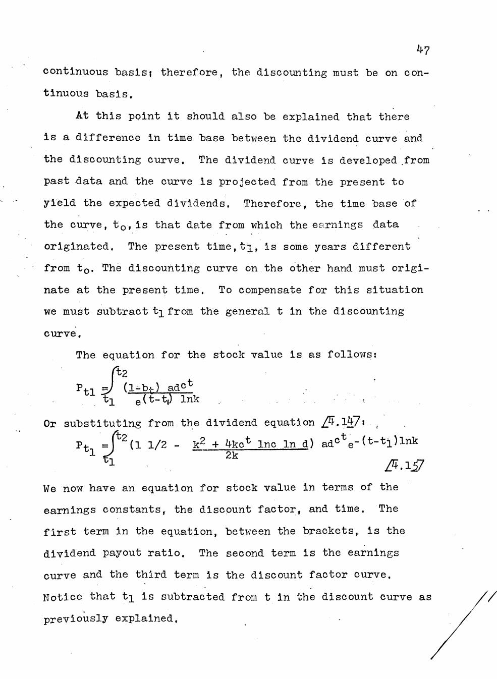
continuous basisj therefore, the discomiting must be on con-

tinuous basis.

At this ppint it should also be explained that there

is a difference in time base between the dividend curve and

the discoimting curve. The dividend curve is developed .from

past data and the curve is projected from the present to

yield the expected dividends. Therefore, the time base of

the curve, tø, is that date from which the earnings data

originated. The present time,ti, is some years different

from tø. The discouhting curve on the other hand must origi-

nate at the present time. To compensate for this situation

we must subtract t^ from the general t in the discounting

curve,

The equation for the stock value is as follows:

rt2 Ptl5/ (l--bt) adC^

tl e(t-t,) Ink

Or substitutlng from the dlvidend equation /JÍ.l}£/\ ,

Ptn = *^(1 1/2 - k^ + ^Ke^ Inc In d) ad°*e-(*-''=l)l' ^ 2k

Me now have an equation for stock value in terms of the

eamings constants, the discount factor, and time. The

first term in the equation, between the brackets, is the

dividend payout ratio. The second term is the earnings

curve and the third term is the discount factor curve.

Notice that t^ is subtracted from t in the discount curve as

previously explained.

48

The upper limit of t^, instead of infinity, is placed

on the integral sign for two reasons. One reason is that

the curve cannot be integrated by conventional means. 'Hou-

ever, it can be integrated by computer after the various

constants are foimd for a particulax firm. The integration

can be programmed by either Simson's rule or the trapezoidal

rule. This is a process of summations and even the fast

computers of today 'cannot mak:e infinite siommationsî there-

fore, a finite upper limit must be placed on the integration.

As a practical matter after the growth rate becomes small

th^ amount added to P. is very small because the discount is

very large according to the number of years to t^.

The other of the two reasons is that the investor

would place some limit on the time period in his ovjn mind

after the eamings curve is examined. When the earnings

curve approaches its asjnnptotic limit,. the investor would

not expect the condition to continue indefinitely. By weigh-

ing the nature of the business, the amount added to the

stock price per time period in the remote future and the

nature of the earnings curve, the investor will reach a

conclusion on the future time limit.

Further clarif'ication of this point may be shown by re-

examining the examples of growth rates and discounting in

Chapter II.

49

Conclusion

We now have g^neral equations for the eamings, assets,

dividends, and stock valuation of the firm in a form that

can be calculated from available data. All of the equations

are in the form of the earnings constants, the discount

factor, and time. The earnings constants can be obtained by

a competent statistician. With these relations the inter-

actions of the different variables can be studied in detail.

Any set of constants thát are calculated are subject

%o the constraints of a given set of economic conditions.

When economic conditions change the constants a, d, and c

change, The nevj constants must then be calculated after

enough time has elapsed to obtain reliable data. Economic

conditions in some cases may be too variable to obtain ac-

curate guidelines, Eowever, the majority of the time stable

data should be available. It is assumed that the larger

firm vjill have more stable data than the small firm because

of diversification and more avenues of financing.

The other part of the study that causes concern is the

investment rate or our estimate of b. If the s.tock value

equation could be integrated by conventional means then we

could obtain this rate directly by mathematics. However,

this integration must be made with the aid of the computer.

The computer also gives us the means to test various values

of the irivestment rate. These tests- can produce an

50

investment rate that will maximize stock price. The author

firmly believes that the estimate of b for the lower rates

of returns is correct. When the maximum stock value and the

resultant investment rate are found the equations should

show that the investment rate will approach zero as the.rate

of return approaches the discount factor, k. Other esti-

mates of b, however, should be tested empirically before

the final analysis is made.

51

CHAPTSR V

SUI/IMARY AITD CONCLUSIONS

Summary

In this paper past theories of stock evaluation have

been presented to build a foundation for the erection of

the non-linear model, A large part of the work by previous

authors on stock evaluation has been directed tovjard the

examination of the linear stdck model. The essential parts

of the linear model have been presented to show its applica-

tions and the assumptions on vjhich it is based. The princi-

pal assiimption of the linear modeí is that the firm vjill

have infinite grovjth at a constant rate. In the world of

reality this, of cours^, cannot be true. To temper this

assumption some of the authors suggested that the far dis-

tant future would have little effect on the model. It was

shovm in Chapter II that the distant future has a very

definite effect on the calculated value of the stock by the

use of the linear model, It is difficult to perceive that

the thoughtful investor would use the linear model to evalu-

ate an investment in common stock.

However, the work done on the linear model has opened

insights toward other evaluations of comjnon stock. The vjork

defining grovith, investment rate, and the discount factor has

laid the foundations of investment theory.

52

53

Williams was the first to present a non-linear stock

evaluation model. The primary thesis of his chapters on

stock evaluation vjas that the dividends of the firm vjould

experience fast growth in the early years, but that the

growth would diminish and approach asymptotically some upper

limit.

The important aspects of the model presented in this

paper are not just stock evaluation but the mathematical

def inition of a niMber of thé more important internal fi-

nancial factors of the firm. An evaluation of the firm's

stock is a result of these internal factors.

The primary assumption of this model is that earnings

growth will be consistent with the Lavj of Variable Pro-

portions. The curve developed for the pro^ected earnings

of a firm is only one curve that may be used in projecting

these eamings, ..Any curve conceived by the investor may be

used for the projection of eamings of the firm as long as

the curve is consistent with economic theory. Of course,

this statement does not give license-to the linear model,

because the assmption of the linear model of infinite growth

is not consistent with economic theory, The slope of the

projected curve is the important item in determlning the

financial factors of investment rate, rate of return, assets,

dividends, and stock evaluation of the firm,

The equations for the financial factors of earnings.

54

assets, dividends, stock evaluation, investment rate, and

rate of return are developed in terms of the earnings curve

constants, the rate of return that investors require, and

time. These equations show mathematically the interrela-

tions of these financial factors of the firm. The.investor

and the firm must make a determination of the future earn-

ings of the f irm and the rate at which the dividends are to

be discounted to determine the value of the investment.

Application of the Gompertz Curve

The Gompertz Cijrve as presented is b.ased on a law of

economics. The lavj is based on a given set of economic

conditions. The conditions can change at any time and the

firm will face a new set of constants. A new firm is usu-

ally subject to more change than an old firm. Hence, greater

caution should be applied to the curve in the early years of

the firm, The older firm,' with more stable conditions, can

place more reliance on the predictions that result from the

use of the curve.

If management uses the model every day for financial

decisions, pressure for change will be brought to bear on

the older firm because of the knowledge that the firm is ap-

proaching a static condition. The firm will have a picture

of the condition it faces. This picture can be balanced

against the risk of change.

55

Another important aspect of the curve is its use for

control purposes. Extraordinary deviations of earnings

from the pro,3ected curve can be detected. Upon detection of

the deviation a search can be made to find the root cause.

The cause can then be corrected, if necessary. In.-some

cases the cause may not be correctable under existing con-

ditions. However, the cause will be known and thus can be

considered vjhen decisions are made.

Since the growth rate of the curve is down trending,

decisions baséd upon it should be relatively conservative.

As' shown in Figure .4, Chapter IV, the semi-log graph, the

slope gradually decreases. This shows that the grovjth rate

will not continue and that dividends will not continue to

increase above a given level. This situation should yield

a definitive investment picture that is conservatively

based. Ho.wever, let us emphasize . that a projection of the

curve is not conservative, but that this is the maximum the

firm can pbtain under the economic law. The firm can do

far worse.

Application of the Model

The investor and the firm should flrst determine the

future earnings 6f the firm either by the Gompertz Curve as

presented in this paper or by any other method that is con-

sistent with economic theory. After future earnings are

56

determined, the discount factor must be determined. In the

case of a firm in which the stock is publicly held and quo-

tations on the stock are made regularly, the discount

factor may be estimated from the market data. This discount

factor may then be checked against the discount factor im-

plied in the actual investment rate and rate of return of

the firm. There no doubt will be a difference between the

two discount factors, An evaluation can then be made be-

tween the evaluator's estimate of eamings and the market

estimate of eárnings, The investor can then evaluate the

stbck for investment purposes. The firm can use the data

to maximize the value of the stock,

For the firm that is privately held, the required rate

of return may be determined in advance. The managers may

then apply the model developed as a control device. The

use of th'e control model will detect changes from normal in

the financial factors and corrective measures may be insti-

tuted if required.

Implications of the Model

In previous models, the investment rate and the rate

of return of the firm have not been shovjn'as variables.

The equations developed in this. model show these factors as

variables that are dependent on the rate of return that in-

vestors-require and the slope of the earnings curve.

57

Speclfically the investment rate equation shows that the

greater the slope of the earnings curve the greater will be

the rate of investment. The equation for investment rate,

b = -k +|/k + kc" In d Inc. /5.l7 2k

is consistent with reality in that the more investors can

make from an investment the more they will invest. This

may seem a simple statement,. but it has not been recognized

in previous models. Another important part of the invest-

ment rate equation is that as the earnings approach a given

level the investment rate approaches zero-. Thiîs is signifi-

cant in that assets will not be increased beyond the point

where the yield rate is below the rate of return that in-

vestors require. The equation for the investment rate con-

tains both of these elements. As previously explained it

may not y-ield maximum stock price, but it is consistent with

reality. Other tests of tbe investment rate through empiri-

cal work or through theory may yield the equation that

maximizes stock price.

The equation for the rate of return.

r = k +l/k + 4kc^ Ind Inc.

2 ; ^ /5,27

shows that it will approach the rate of return that investors

require when the slope of the earnings curve approaches zero.

This is consistent with the requirement for the investment

rate in that investors will invest up to the required ratQ

58

but not beyond that point. The rate of return equation is

also dependent on the slope of the earnings curve in that

the rate of return has to be greater than the required rate

before the firm will grow. This requirement is implied in

the estimate of future earnings, because there will" be no

growth in eamings or assets unless the rate of return of

the firm is greater than the required rate.

These two variables, the investment rate and the rate

of return of the firm, are the key elements in finding the

othér financial variables. The asset requirements are the

earnings divided by the rate of return of the firra. The

dividends of the firm are the earnings less the investment

rate times earnings. V/ith the dividends defined, the stock

value is the summation of the dividends discounted at the

rate of return that investors require. Therefore, the fi-

nancial variables of assets, dividends, and stock price are

the result of finding (l) the estimate of earnings, (2) the

rate of return that .investors require, and (3) the rate of

return of the.firm and the investraent rate of the firm. The

rate of return and the investment rate are combined to show

that-one is dependent on the other, because the multiplicand

of the two is equal to the slope of the earnings projection. >

From this summary some important points may be gleaned.

The first is that the rate of return of the firm must be

greater than the rate of return that investors require before

59

the firm will grow in either earnings or assets. Following

this line of reasoning further, vjith growth in earnings, the

dividend rate will grow and, hence, the stock price, The

implication of the above statement is that the rate of re-

turn of the firm is the key to the growth of stock price.

This we know is a true statement. The model developed in

this paper exhibits all of these characteristics. It ex-

hibits grovjth in earnings, assets, dividends, and stock

price as long as the rate ofreturn is greater than the

r.ate investors require. Also the model exhibits growth that

is consistent with economic theory.

Conclusions

The earnings curve is a fair ^udgment of the financial

future of the firm at any given point in time. Yet as

Williams pointed out, the general shape of the curve is the

maximum value thát the eamings can achieve for a given set

of economic conditions.^^ Reassessment of the parameters

of the curve should be continuous so that deviations can be

detected. The root cause of the deviations should be exam-

ined for possible action.

Stock price valuation can be made, based on more than

Judgment by the use of the mathematical data. A plot of

29 Williams, Investment Value, p. l4l.

60

stock price can be made from the data. This vjill give the

computed price of the stock at any given point in time.

Deviations from stock price should be examined for possible

action, The other financial activities, level of assets and

dividend payments, can be predicted and plans made for

changes. The firm can plan for raaximum stock price.

As presented in this paper only the theory of the model

has been examined. Empirical work on each of the financial

factors of the model should be applied before confidence is

established in the use of the model. Deviation from the

theory should be critically examined.

The theory does give a mathematical, concise guide for

action that conforms more to reality than does the theories

of the past.

BIBLIOGRAPHY

Books

Bober, M. M. Intermediate Price and Income Theory. Revised Edition. New York: W. W. Norton « Company, Inc., 1955.

Britt, Stevjart Henderson, and Boyd, Harper W. , Jr. Marketing Manap^ement and Administrative Action. îlew York: McGraw-Hill Book Company, '1963

Gordon, Myron J. The Investment. Financing and Valuation of the Corporation. Homevjood, 111.: Richard D. Irwin, Inc. , I96T.

Lerner, Eugene M. , and Carleton, Willard T. A Theory of Financial Analysis, New York: Harcourt, Brace & Uorld, Inc, 19657~ "

Solomon, Ezra. The Managem.ent of Corporate Capital. Gencoe, 111.: Free Press, 1958.

Stockton, John R. Business Statistics. 2nd ed. Cincinnati, Ohio: Southvjestern Publishing Company, I962.

Weingartner, H. Martin. Mathematical Programming and the Analysis of Capita]. Budgeting Problems. Englewood Cliffs, N.J.: Prentice flall, l ' Jl

Articles

Bernoulli, Daniel, Exposition of a New Theoryon the Measure-ment of Risk," Economitricá. XXII (1954), 23-26. Trans-lated by Dr. Louis Sommer of Bernoulli's paper, Specimen Theorical Novae de Mensura Sortis, Commentarii Aca demiae Scientiariun mperialis Petropolitanae, V (1738). 175-92.

Bodenhorn, Diran. "On t'ne Problem of Capital Budgeting." The Journal of Finance."Vol. XIV (December, 1959), 473-92.

Boumol, W. J. , and Quandt, R. E. "Mathematical ProgramiQÍng and the Discount Rate Under Capital Rationing." Sco-nomic Journal (June, I965), 317-29,

61

62

Buckley, Julian G, "A Method of Evaluating Grovjth Stocks." Finanoial Analyst Journal. Vol. XVI (Karch-April, I96O), 19-21.

Burrell, 0. K. "A Mathematical Approach to Growth Stock Vaiuation," Financial Analysts Journal. Vol. XVI (May-June, 1960), 69-76.

Clendenin, John C. , and Van Cleeve, Maurice, "Grovjth and Common Stock Values." The Journal of Pinance, Vol. IX (1954). 'b65-'l(^,

Durand, Davis. "Grovjth Stocks and the Peterburg Paradox. " The Journal of Finance. Vol. XII (September, 1957).

Holt, Charles C. "The Influence' of Growth Duration on Share Prices." The Journal of Pinance. Vol. XVII (September, 1962), 465-77.

Modigliani, Franco, and Miller, Merton. "The Cost of Capi-tal, Corporation Finance, and the Theory of Investment." American Economic Review (June, 1958).

Walter, James E. "Dividend Policies and Common Stock Prices." The Journal of Finance. Vol, XI (March, 1956), 29-4l.