aurel carcoana - applied enhanced oil recovery
DESCRIPTION
petroleum engineeringTRANSCRIPT

Library of Congress Cataloging-in-Publication Data
Carcoana, Aurel. Applied enhanced oil recovery I Aurel Carcoana.
p. em. Includes bibliographical references and index. ISBN 0-13-044272-0 1. Secondary recovery of oil. I. Title.
TN871.37.C37 1991 622'.33827-dc20
Editorial production supervision and interior design: Laura A. Huber
Production assistant: Jane Bonnell Acquisitions editor: Michael Hays Editorial assistant: Dana L. Mercure Prepress buyer: Mary Elizabeth McCartney Manufacturing buyer: Susan Brunke Copy editor: Sally Ann Bailey Cover artist: Karen Stephens Marketing manager: Alicia Aurichio
© 1992 by Prentice-Hall, Inc. A Simon and Schuster Company Englewood Cliffs, New Jersey 07632
The publisher offers discounts on this book when ordered in bulk quantities. For more information, write: Special Sales/Professional Marketing, Prentice Hall, Professional & Technical Reference Division, Englewood Cliffs, NJ 07632.
All rights reserved. No part of this book may be reproduced, in any form or by any means, without permi!lsion in writing from the publisher.
Printed in the United States of America 10 9 8 7 6 5 4 3 2 1
ISBN 0-13-044272-0
Prentice-Hall International (UK) Limited, London Prentice-Hall of Australia Pty. Limited, Sydney Prentice-Hall Canada Inc., Toronto Prentice-Hall Hispanoamericana, S.A., Mexico Prentice-Hall of India Private Limited, New Delhi Prentice-Hall of Japan, Inc., Tokyo Simon & Schuster Asia Pte. Ltd., Singapore Editora Prentice-Hall do Brasil, Ltda., Rio de Janeiro
91-26308 CIP
ISBN D-13-044272~~
9 o o ao~
9 780130 442727
Contents
PREFACE xiii
ACKNOWLEDGMENTS XV
NOMENCLATURE XX
SUBSCRIPTS XXV
CONVERSION FACTORS xxvii
1' HYDROCARBON CLASSIFICATION AND OIL RESERVES 1
1-1 Hydrocarbon Classification 1
1-2 Oil Reserves Classification 3 Recovery Possibilities, 3 Degree of Proof, 3 Development and Producing Status, 4 Energy Source, 4
Questions and Exercises 7
References 7
v

vi
2 PRODUCING RESERVES
2-1 Oil Recovery Methods 8
2-2
2-3
Primary Recovery Methods, 8 Improved Recovery Methods, 8
Enhanced Oil Recovery Methods 9
Oil Recovery Factor 11
Questions and Exercises 14
References 15
3 STEAM: A HEAT CARRIER AGENT
3-1 Liquid to Vapor Phase Change 16 Boiling Point, 17 Vaporization Point, 17 Water-Steam Pressure-Volume Diagram, 18
3-2 The Heat Content of Steam 19 Steam Enthalpy, 119 Steam Tables and Charts, 21 Steam Quality, 23
3-3 Wet Steam Generators 26
3-4 Feedwater Treatment 28
3-5 Heat Losses 29 Steam Generator Heat Loss, 30 Heat Loss on the Surface Transmission Lines, 31 Heat Loss from the Wellbore, 31 Downhole Steam Generator, 35 Reservoir Heat Loss to Adjacent Formations, 36
3-6 The Heat Effect on Reservoir Oil Viscosity 36 Questions and Exercises 38
References 39
4 STEAM INJECTION
4-1 General 41 4-2 Processes Description and Recovery
Mechanisms 42 Steam Drive Process, 42 Cyclic Steam Injection Process, 44
4-3 Heat Amount to the Formation 47
8
16
41
Contents
I I I
Contents
4-4
4-5
4-6
4-7
Heated Radius 49
Steam Drive Displacement 50 Oil Displacement Rate, 50 Oil Recovery, Oil Steam Ratio, 55
Cyclic Steam Injection 59
Field Development and Results 61 Kern River Steam Foam Pilots, California, United States, 62 The "200" Sand, Midway Sunset Steamflood, California, United States, 65 Pikes Peak, High-Viscosity Oil Reservoir, Canada, 69 Tar Sand Steam Injection, 73
4-8 Screening Criteria 75
Questions and Exercises 77 References 77
5 IN SITU COMBUSTION
5-1 General 80
5-2 Laboratory Studies 81 Oxidation Cells, 81 Combustion Tubes, 82
5-3
5-4 5-5 5-6
5-7
5-8
5-9
5-10
Qualitative Description of In Situ Combustion 84
Wet Combustion 86
Reverse Combustion 87
Combustion Parameters 88 Description, 88
Calculations 88
Area of Application and Pilot Tests 91 Reservoir and Fluid Characteristics, 91
Pilot Tests, 92
Field Development 94 The Moco Zoo, California, United States, 95 Suplacu de Barcau, Romania, 97 Heidelberg Field, Mississippi, United States, 107
Pattern Sweep, Invasion, and Displacement Efficiencies 111 Sweep Efficiencies, 113
vii
80
viii
5-11
5-12
5-13
5-14
5-15
Oil Consumed In Situ 114
Oil Recovery 116 Screening Criteria 120 Reservoir Characteristics, 120
Injection of Oxygen-Enriched Air or Pure Oxygen 121 Design of an In Situ Combustion Field Pilot 122 Questions and Exercises 129
References 131
6 POLYMER FLOODING
6-1 General 135
6-2
6-3
6-4
6-5
6-6
6-7
6-8
Principle and Method Description 136 Water and Oil Mobilities, 136 Mobility Ratio Concept, 136 Polymers Reduce Water-Oil Mobility Ratio, 136 Method Description, 138
Polymer Types 140 Polyacrylamides, 140 Polysacharides, 141
Apparent Viscosity and Resistance Factor 141
Apparent Viscosity, 141 Resistance Factor, 142 Residual Resistance Factor, 143
Polymer Retention 144 Adsorption and Entrapment, 144 Molecular Weight and Screen Factor, 144
Field Projects and Results 146 Field Projects, 146 Field Results, 147
Guidelines for Polymer Application 148 Reservoir Characteristics, 148 Fluid Characteristics, 148 Reservoir Selection, 148 Incremental Oil Recovery, 149
Design Considerations 154 Sleepy Hollow Reagan Unit, Nebraska, United States, 155
Questions and Exercises 157 References 158
Contents
135
Contents
7 ALKALINE FLOODING
7-1 General 160 7-2
7-3
7-4
Displacement Mechanisms and Method Description 161 Displacement Mechanisms, 161 Method Description, 163
Design Considerations and Screening Criteria 163 Design Considerations, 163 Screening Criteria, 165
Field Trials 166 Whittier Oil Field, California, United States, 167 Wilmington Field Ranger Zone, California, United States, 170
Questions and Exercises 173
References 173
8 MISCIBLE FLUID DISPLACEMENT
8-1 General 175
8-2
8-3
8-4
8-5
Phase Behavior 176 Phase Change Representations, 176 P-1' Phase Equilibria Diagram, 177 Ternary Diagram, 181 Pseudoternary Diagram, 183
Hydrocarbon-Solvent Miscible Flooding 186 Residual Oil Saturation and IFT, 186 First-Contact or Direct Miscibilitv 186 Multiple Contact or DynamicMi;;ibility, 188
Field Development of Hydrocarbon-Solvent Flooding 191 Rainbow Keg River "B" Pool, Alberta, Canada, 191
Westpem Nisku D Reef, Alberta, Canada, 196 Block 31 Field, Texas, United States, 198 Hassi-Messloud Field, Algeria, 199
Screening Criteria 199 The Oil Viscosity and Gravity, 200 Reservoir Pressure and Depth, 200 Reservoir Geometry, 200 Oil Saturation at Start of the Project, 201 High-Risk Factors, 201
Questions and Exercises 201 References 202
ix
160
175
X
9 MICELLAR-POLYMER FLOODING
9-1 General 203
9-2 Principle and Method Description 204
Principle and Characteristics, 204 Pseudoternary Diagram, 204
9-3
9-4
9-5
9-6
9-7
Method Description, 205
Laboratory Experiments 206 Experimental Conditions, 206
Field Test Projects 208
The M-1 Project, Illinois, United States, 208 The Loudon Pilot, United States, 212
Screening Criteria and Critical Quantities 213
Screening Criteria, 213 Critical Reservoir and Micellar Quantities, 214
Preliminary Economic Evaluation Model 216
The Chemical Flood Predictive Model 226
Questions and Exercises 229
References 230
10 CARBON DIOXIDE FLOODING
10-1 Properties of C02 232
10-2 Factors that Make C02 an EOR Agent 234
10-3 C02 Miscible Flooding 237
Multiple-Contact Miscibility, 237 Miscibility Pressure, 238
10-4
10-5
10-6
COz Immiscible Flooding 241
Design Considerations 241
General, 241 Flood Design and Performance Predictions, 242
C02 Demand, Sources, and Transportation 248 C02 Demand, 248 C02 Sources, 248 Transportation of C02, 249
10-7 Field Projects 249 -'-< _
Operational Problems, 250 Miscible C02 Flood Kelly-Snyder Field, 250 SACROC Unit, Texas, United States, 251 CO;r WAG Project, 255
Contents
203
232
Contents
Four and Seventeen Pattern Areas, 256 Immiscible C02 Project, Tar Zone, Wilmington Field, California, United States, 258
Questions and Exercises 262
References 263
11 OIL MINING, MICROBIAL EOR, AND ELECTROTHERMAL PROCESSES
11-1 General 266
11-2
11-3
11-4
Oil Mining Methods 267
Historical, 267 Oil Mining in the United States, 267
Microbial EOR 271 General, 271 New Developments and Field Tests, 272
Electrothermal Processes 276
Questions and Exercises 277
References 277
12 EOR COULD OFFSET OIL PRODUCTION DECLINE
12-1 Energy Consumption 279
12-2 Energy Supply 280
12-3
INDEX
Domestic Crude Oil Production, 280 Foreign Sources, 282
EOR: The Answer for Offsetting Oil Production Decline 282
References 285
xi
266
279
287

Nomenclature
A a a
B b
c c Ca
XX
Area, acres, ff
Geothermal gradient, °F/ft
Well-to-well spacing, ft (Eq. 5-19)
Active surfactant retention, mg/g rock (Eq. 9-7)
Formation volume factor, bbUSTB
Surface geothermal temperature, oF (Eq. 3-10)
Constant (Eq. 3-6)
Specific heat capacity, Btu/Ibm x °F or J/kg x °C.
Amount of air required to bum through a cubic foot of reservoir rock, scf/fe
Amount of coke deposited or fuel content, lbm/fe
Injection pressure gradient, psilft (Eq. 9-1)
Concentration of active surfactant in the injected slug (Eq. 9-7) Volume fraction of pseudocomponent 1 in phase St Surfactant requirements, bbl or m3
Nomenclature xxi
CTP Polymer requirements, bbl or m3
D Depth, ft
D Thermal diffusivity of the cap rock, ft2/hr (Eqs. 4-1 and 4-5) D, Effective diffusion coefficient for C02/oil or N2/C0
2, cm2/s
(Eq. 10-7)
D. Surfactant retention, dimensionless (Eqs. 9-6, 9-14) d Tubing inside diameter, in. (Eq. 10-13) E Efficiency, fraction or percent E Expenses, $
fopk
H
Ho h h
h
h, hg
htg K k k
k k. lv
ln log M M,
Micellar-polymer displacement efficiency, fraction Overall oil recovery factor, percent Fluid volume, bbl
Fraction (such as the fraction of a flow stream consisting of a particular phase)
Friction factor, fraction (Eq. 10-13)
Vertical heat loss, fraction (Eq. 4-11) Steam quality, percent
Dimensionless transient heat conduction time function (Eq. 3-10)
Oil cut or the peak oil rate, volume percent (Eq. 9-20) Heat of combustion, Btu/Ibm or J/kg Heat injection rate, Btu/hr
Formation thickness, ft
Enthalpy, Btu/Ibm or J/kg
Differential pressure, inches of water (Eq. 3-6)
Enthalpy of saturated liquid, Btu/Ibm or J/kg Total enthalpy, Btu/Ibm or J/kg
Enthalpy of vaporization, Btu/Ibm or J/kg
Thermal conductivity of the cap rock, Btu/ft x hr x oF Permeability, md
Thermal conductivity of the earth, Btu/day x ft x oF Mean permeability, md (Eq. 6-6)
Permeability at 84.1 percent of the cumulative samples, md
Specific latent heat (enthalpy) of vaporization, Btu/lb or J&g m
Natural logarithm
Base 10 logarithm Mobility ratio, mixture Empirical function (Eq. 9-17)

xxii
Ms m
P,p
Q Q
Qo
Qf Qg
Qs
Qs
Qv
Qw q R
R
r
s s So(S') T
t
v
Nomenclature
Heat capacity of steam saturated rock, BtuJfe x op
Mass, lbm or kg Oil in place, bbl Capillary number Reynolds number Tubing roughness, in. (Eq. 10-13) Atomic H/C ratio pressure, psi Total heat amount, Btu or joule Total air injected, scf Total injection volume, pore volumes Net amount of heat available to formation, Btu or joule Steam generator heat loss, Btu or joule Sensible heat, Btu or joule Heat lost on surface lines, Btu or joule Latent heat of vaporization, Btu or joule Heat loss rate in wellbore, Btu/day (Eq. 3-10) Rate, bbl/day Resistance factor, ratio Revenue,$ Radius, ft Saturation, fraction Saturation phase (relative amount), fraction Oil price (base), $/STB Temperature, reservoir temperature, °F or oc Time (injection), days, hours Oil breakthrough time, porous volume (Eq. 9-18) Time of peak oil rate, porous volume (Eq. 9-19) Air flux density, scf!fe x hr Overall heat transfer coefficient, Btu/day X ft X op Idem, Btu/hr X ft X op
Superficial or actual velocity, ft/day Volume, bbl Velocity, ft/day Permeability variation (Dykstra-Parsons) Rate of the burning front advance, ft/day Rate at which oil is displaced, bbl/day (Eq. 4-4)
Nomenclature xxiii
v
Vg
w wd Wo
Wp X y
z z DA t:..N
t:..T MD MP
PV RO SG TO AOR API
EOR FPV GOR NRP OSR
SOR
STB TDS TDV WOR
ppg
ppm
CFPM
Volume occupied by gases in reservoir after pressurization, bbl (Eq. 10-3)
Specific volume of saturated liquid, ft3/lbm Specific volume of saturated vapor, fetlbm Flow rate of wet steam, gal/min (Eq. 3-6) Density of dry steam, lbmtfe (Eq. 3-6)
Heat injected lost to adjacent strata, fraction (Eq. 4-2) Cumulative water produced, bbl Length of diffusion zone, ft Mole fraction in combustion gases Gas deviation factor Formation depth, ft (Eq. 3-10) Developed area, acres
Cumulative oil produced during an interval, bbl; reserves (recoverable), bbl Temperature difference, op
Measured depth, ft Micellar-polymer Porous volume, bbl Recoverable oil, bbl Specific gravity Target oil, bbl Air-oil ratio American Petroleum Institute Enhanced oil recovery Floodable pore volume, bbl Gas-oil ratio
Number of repeated patterns Oil-steam ratio Steam-oil ratio Stock tank barrels Total dissolved solids, ppm True vertical depth, ft Water-oil ratio
Parts per gallon Parts per million
Chemical flood predictive model

xxiv
CRMQ HCPV OOIP PEC<!>N <I>
X.
'"" p
'T
Critical reservoir and micellar quantities Hydrocarbon pore volume, bbl Original oil in place, bbl Preliminary Economic Evaluation Model Porosity, fraction or percent Mobility, md/cp Viscosity, cp Density, lbm/fe or g/cm3
Interfacial tension (IFT), dyne/em
Nomenclature
Subscripts
a air, actual, areal A areal b burning c combustion, caprock cons consumed cr critic d dry, diffusion D dimensionless, displacement e effective, external ext exterior feedw feed water g gas h heated
initial, injection I invasion, vertical inj injected
XXV

xxvi
int
MB max min 0
ob of om or ore orw ov p pp r s T tf ts u v w wb wf ws
interior liquid mobility buffer maximum minimum initial, oil oil bank oil formation mobil oil residual oil micellar-polymer swept zone residual oil residual oil after waterflooding overburden polymer, produced, pattern pressurization phase relative, rock, residual surfactant, specific, solid, soluble, steam
total tubing flowing (pressure) tubing static (pressure) unburned zone volumetric water, wet, well water bank bottom well flowing (pressure) well static (pressure)
Subscripts
Conversion Factors
acre = 4046.856 m2
acre-ft = 1233.482 m3
atm = 101.325 kPa = 0.101325 MPa = 14.696 psi bbl = 42 u.s. gal = 5.614583 fe = 0.158987 m3
bbVacre-ft = 0.128893 m3/m3
Btu = 10505.056 J = 251.996 cal Btulfe = 37.259 kJ/m3
Btu/hr = 0.293071 W Btullbm = 2.326 kJ/kg Btu X lbm -l X op- 1 = 1 kcal X kg- 1 X K- 1 = 4.186800.kJ X kg- 1 X K- 1
cal = 4.186800 J cp=1mPa·s Darcy = 0.986923 f.Lm2
dyn/cm = 1 rn.N/m ft = 0.304800 m fe = 9.290304 X 10⁻² m2
xxvii

xxviii
fe = 2.831685 X 10⁻² m3
fe/bbl = 0.178108 m3/m3
Conversion Factors
gal (U.S.) = 3.785412 dm3 or liters = 3.785412 X 10⁻³ m3
in. = 2.540 em = 0.025400 m Ibm = 0.453592 kg lbmtfe = 16.018463 kg/m3
psi = 6.894757 kPa = 6,894. 757 Pa = 6.894757 x 10⁻³ MPa
ton = 1~ kg
Hydrocarbon Classification and Oil Reserves
1-1 HYDROCARBON CLASSIFICATION
Chapter 1
There is a large number of hydrocarbon compounds with molecules composed of the chemical elements hydrogen and carbon in various proportions.
Hydrocarbons will exist in a fluid phase (gas or liquid) or as solids in a reservoir, depending upon changes in temperature or pressure.
Fluid hydrocarbons or petroleum are normally produced through wells and are subdivided into liquid hydrocarbons and natural hydrocarbon gases. The recommended classification and nomenclature of the fluid hydrocarbons (Arps, 1962; SPE, 1981) is provided in Figure 1-1, with SPE letter symbols standard (SPE, 1986).
Liquid hydrocarbons are subdivided into the following categories:
Crude Oil: "a mixture of hydrocarbons that exists in the liquid phase in natural underground reservoirs and remains liquid at atmospheric pressure after passing through surface separating facilities."
Natural Gas Liquids: "those portions of reservoir gas that are liquefied at the surface in lease separators, field facilities, or gas processing plants.
1

2 Chap. 1 Hydrocarbon Classification and Oil Reserves
Fluid Hydrocarbon Classification
I Crude Oil, N
Uq";d Hydmwboo. K .--.....::..----.
Natural-Gas Liquids, NGL
Condensate, C L
Gasoline, CLg
Liquefied Petroleum Gases, C Lp( LPG)
Flu id-Hyd rocarbo ns
Fig. 1-1 Fluid hydrocarbon classification
Nonassociated Gas, G
Associated Gas, Ga
Dissolved or Solution Gas, Gd
Injected Gas, Gi
Natural gas liquids include but are not limited to ethane, propane, butanes, pentanes, natural gasoline, and condensate."
Natural Gas: "a mixture of hydrocarbons and varying quantities of nonhydrocarbons that exists either in the gaseous phase or in solution with crude oil in natural underground reservoirs." Natural gas is subdivided into the following categories:
Nonassociated Gas: natural gas that is in reservoirs that do not contain significant quantities of crude oil.
Associated Gas: natural gas, commonly known as gas-cap gas, which overlies and is in contact with crude oil in the reservoir.
Dissolved Gas: natural gas in solution with crude oil in the reservoir.
Sec. 1-2 Oil Reserves Classification 3
Injected Gas: gaseous hydrocarbons that have been injected in underground reservoirs for pressure maintenance or storage purposes.
The scope of this book is limited to crude oil as it occurs in the natural liquid phase under reservoir temperature and pressure and the problem of how to recover more of the original oil in place .
1·2 OIL RESERVES CLASSIFICATION
The oil reserves classification takes into consideration the following criteria:
• Recovery possibilities • Degree of proof • Development and producing status • Energy source
Recovery Possibilities
The recovery possibilities refer to the fact that the amount of oil produced from original oil in place (OOIP) is limited by existing recovery mechanisms, efficiency of known reservoirs, and economic conditions.
Degree of Proof
The OOIP which initially saturates the porous space of the rock reservoir is difficult to determine exactly in the beginning (the exploration phase), when minimal information is available. Knowledge of the amount of original oil in place is improved by volumetric or material balance calculations at the start of development and during the exploitation of the oil reservoir. However, cumulative oil production obtained and measured at surface conditions can be accurately determined.
If N is the amount of original oil in place (barrels, bbl, of oil) and tiN is the cumulative oil produced (bbl) at a given time, the ratio ER = tiN x 100/N % is the oil recovery factor at that time or the actual oil recovery factor.
The petroleum engineer is mainly interested in knowing from the beginning the ultimate oil recovery from a reservoir, in other words, the product N X ERfinai' where ER6 •• 1 is the ultimate recovery factor. During the early stages when few data are available, but when important decisions regarding the development of the reservoir must be made, and during the life of a reservoir the term "recoverable reserves" or simply
reserves = tiN = N X ERr. •• ,
should be estimated with more and more acc~racy.

4 Chap. 1 Hydrocarbon Classification and Oil Reserves
J. J. Arps ( 1962) shows three periods in the life of an oil reservoir. In the first period, before any wells are drilled, a general estimation of reserves in barrels per acre is made based on experience. In the second period, the first wells drilled are produced. The amount of original oil in place, N, is calculated on a volumetric or material balance basis and ERfin•I is estimated knowing the principal recovery mechanism. The reserves are expressed in barrels per acrefoot or barrels. In the third period a performance decline trend curve can be extrapolated or a mathematical model made matching the past performance of the reservoir. The reserves are estimated in barrels.
It is evident that the estimated reserves must have a degree of proof or certainty specific to each phase when the estimation is made.
Development and Producing Status
It is also necessary to consider development status to distinguish between reserves recoverable through existing wells and "reserves" under undeveloped spacing units. These are "so close and so related to developed spacing units that they may be assumed with the same certainty to be produced when drilling" (Arps, 1962).
Producing status is the highest status of reserves because the oil reserves are produced through the existing wells and/or are expected to be recovered from existing wells. Producing reserves are the result of the natural energy source inherent in the reservoir or supplemented by artificial means.
Taking into consideration recovery possibilities, the degree of proof, the development status, and the producing status criteria, a classification of oil reserves is given in Figure 1-2.
The United States has already produced 139 billion bbl of oil. This represents an average actual recovery factor of 28 percent from a total of 492 billion bbl of OOIP discovered (Brashear, 1988).
Estimation of currently proven reserves of approximately 28 billion bbl raises the average oil recovery factor from 28 to 34 percent. This represents an ultimate value as the result of current primary and conventional recovery methods.* We can see now that proven reserves are reserves recoverable using different recovery methods or mechanisms. These are developed by the energy source which displaces the oil through the reservoir to the producers. Thus it is important that oil reserves be classified also by energy source criteria.
Energy Source
In an oil reservoir, production results from a mechanism which utilizes existing pressure. This is the source of driving energy. The reservoir having primarily a natural recovery mechanism that uses principally the liberation and expan-
• Approximately 5 percent of the oil produced per year in the United States is however the result of thermal recovery and other enhanced oil recovery (EOR) methods.
Sec. 1-2 Oil Reserves Classification
Oil Reserves Classification
and EOR Target and Path
Criteria
@Producing
/ {!)Developed~ / /"" ""' @Proved @Non producing
reserves
/ ( "- @u,dmlopod
@Reserves / @Probable
(recoverable) -- reserves I,.%. \ I G)OOIP
(100%) @Possible
reserves
)
LEGEND
Unproved reserves
C) EOR Target
- EOR Path
5
@=Original Oil in place,N
®=Estimated volumes of hydrocarbon anticipated to be commercially
recoverable from known accumulations
@=Are less certain than probable
reserves and more likely not to be
recovered
@=1-2
@=Are recoverable reserves under current
economic conditions
@=Are less certain than proved reserves, more likely to be recovered than not
(!)=Are expected to be recovered from existing wells
@=4-7
@=Are expected to be recovered from completion Intervals open at the time
of the estimate and producing
@)=7-9
Fig. 1-2 Oil reserves classification and EOR target and path

6 Chap. 1 Hydrocarbon Classification and Oil Reserves
sian of dissolved gas is termed a "dissolved gas drive reservoir," one that uses principally the expansion of a cap of free gas over the oil zone is termed a "gas-cap drive reservoir," and one that uses principally the influx of natural water is a "water drive reservoir." Driving energy may be derived also from gravity and from combinations of these mechanisms. An oil reservoir with a primary energy source produces oil using one or more of the primary recovery mechanisms just defined.
When oil recovery involves the introduction of energy into a reservoir by injecting gas or water under pressure, the oil is produced by secondary or so-called conventional recovery methods. Waterflooding has been and continues to be very successful and improves the recovery of oil from known reservoirs.
Despite the improvement made in the technology and methods used for development and production of oil reservoirs, a substantial amount of oil, nearly 325 billion bbl or 66 percent of OOIP, remains as droplets trapped in the pores of reservoir rock or as films partly coating the pore walls. Entrapment of the remaining oil is due mainly to capillary forces and interfacial tensions and to a partial sweep of the reservoir by injected fluids. These remaining or nonrecoverable reserves are the target of more sophisticated and expensive so-called enhanced oil recovery (EOR) methods.
Considering the energy source criteria for oil reserve classification, we can conclude that
Primary reserves are reserves recoverable commercially with current equipment and under current economic conditions as a result of primary recovery methods using the natural energy inherent in the reservoir (Arps, 1962).
Secondary reserves are reserves recoverable commercially under current economic conditions, in addition to the primary reserves, as a result of supplementing by conventional methods (water and/or gas injection) the natural energy inherent in the reservoir (Arps, 1962).
Tertiary reserves are reserves beyond those proved recoverable by conventional methods but recoverable by EOR methods.
Each of these categories could be subdivided into proved, probable, and possible; developed and undeveloped; and producing and nonproducing, depending on the information available at the specific time when the reserve estimation is made.
Changes in reserves take place each year and are assigned to newly discovered petroleum reservoirs, extensions of existing reservoirs, and revisions (Lovejoy and Homan, 1965). This last category results from improved knowledge of the geological characteristics of the reservoir and of the implementation of conventional and EOR methods. The goal of the geologist
Questions and Exercises 7
and the petroleum engineer is to promote more proved, developed, and producing reserves. The proved, developed, and producing reserves assure the oil production of the United States.
QUESTIONS AND EXERCISES
1-1 In what phases may the fluid hydrocarbons N, NGL, and G exist in reservoir conditions?
1-2 How are OOIP, ER, and ERfi~' defined? 1-3 Calculate the "reserves" of an oil reservoir knowing the OOIP and the ultimate
oil recovery factor.
1-4 Assuming a cumulative oil production of 853,000 bbl, the amount of original oil in place 7.6 x 10⁶ bbl and the ultimate oil recovery 28 percent, calculate the remaining reserves.
1-5 Define oil reserves by energy source criteria.
REFERENCES
ARPS, JAN J., Petroleum Production Handbook, T. C. Frick, ed. (Richardson, TX: Society of Petroleum Engineers, AIME, 1962), Volume XI, Chapter 37, p. 37-1.
BRASHEAR, J.P., A B. BECKER, and K. H. BIGLARBIGI, "Incentives, Technology, and EOR: Potential for Increased Oil Recovery at Lower Oil Prices," SPE 17454, California Regional Meeting, Long Beach, CA, March 23-25, 1988.
LOVEJOY, W. F., and P. T. HOMAN, Methods of Estimating Reserves of Crude Oil, Natural Gas and Natural Gas Liquids (Baltimore, MD: Johns Hopkins University Press, 1965).
SPE, "Society Adopts Proved Reserves Definitions," Journal of Petroleum Technology, (November 1981), pp. 2113-14.
SPE, SPE Letter and Computer Symbols Standard (Richardson, TX: Society of Petroleum Engineers, 1986).

Chapter 2
Producing Reserves
2-1 OIL RECOVERY METHODS
Close examination of producing reserves is revealing and helpful in classifying the oil recovery methods by energy source criteria.
Primary Recovery Methods
Producing reserves are called "primary" when they are produced by primary recovery methods using the natural energy i~herent in the. reserv~ir. The driving energy may be derived from the liberatwn a~d expa~s10n of dissolv~d gas, from the expansion of the gas cap or of an active aqmfer, from gravity drainage, or from a combination of these effects.
Improved Recovery Methods
The producing reserves are called "improved recovery reserves" when they are produced by improved recovery methods, in addition to the primary reserves,
Sec. 2-2 Enhanced Oil Recovery Methods 9
using additional energy. Improved recovery methods are subdivided into
Conventional methods (secondary ethods), which involve the injection of gas and/or water into the reservoir , and Enhanced oil recovery methods (tertiary methods), of which thermal, chemical , and miscible methods are generally recognized as the most promising.
Primary and improved recovery methods are presented in Figure 2-1. The object of this book is to cover the processes involved in enhanced
oil recovery. The EOR target and path shown in Figure 1-2 is better understood now. It is a difficult and complex path
• from research and lab experiments, which can improve the possible reserves, • through field pilot tests , which can increase the probable reserves , • to proved and producing reserves when the commercial development of the
reservoir under one of the EOR methods is in place.
2-2 ENHANCED OIL RECOVERY METHODS
Since the early 1950s, a significant amount of laboratory research and field testing has been undertaken , and some of the resulting findings have been developed on a commercial scale. The intent of enhanced recovery methods (La til et al., 1980) is to
• improve sweep efficiency by reducing the mobility ratio between injected and in-place fluids ,
• eliminate or reduce the capillary and interfacial forces and thus improve displacement efficiency, and
• act on both phenomena simultaneously.
The basic principles of the most promising EOR methods used are given in Table 2-1.
Other processes, such as bacterial activity, electrical heating of the reservoir, and so on have been proposed, but their potential for adding to proved oil reserves must be demonstrated.
Chemical methods of enhanced oil recovery are characterized by the addition of chemicals to water in order to generate fluid properties or interfacial conditions that are more favorable for oil displacement . Polymer flooding, using polyacrylamides or polysaccarides, is conceptually simple and inexpensive, and its commercial use is increasing despite the fact that it raises potential production by only small increments. Surfactant flooding is complex , requiring deta~led laboratory testing to support field project design. It is also expensive

.. " 0 % .. .. :I ,.. a: .. > 0 u .. a:
" .. > 0 a: ... :I
" z c ,.. a: c :I i ...
• c 0 = • c ... • 0 » .c c -0 • u :I
"'- .. I c u ~ ... 0
.t
c .2 u . :§'
~ . iii u
u
"" u
. ~ . ::
- . . ~ . . . . . . . . . :.a.:. g;~~ ... a:-' \//
\V \t t/ \VI - . . ... e o ~ .c . -.c • .. 2
'ii • u ... - 0 e .c . -.c • u :I
. :;;
~ i
. ~ e ~ ! ~ c N
~ 0 u . c :§' .2
N'; 0 0 u "' v . :;; -;; ~ . . e e e • u - • N'ii, 0 . u 'ii
"' "0 0 ..c 0 . e ... >-! .. <) . i5 :I .. u
c <)
;: .. e "0
<) e > 0 ;; .. ... 0. .§ "0 c "' ~ "' e ·c !:I. -M
~
Sec. 2-3 Oil Recovery Factor
TABLE 2-1. Methods of Enhanced Recovery
Chemical methods
Miscible methods
Thermal methods
Methods Used
Polymer-augmented waterflooding; surfactant flooding; alkaline flooding; C02-augmented waterflooding; immiscible C02 displacement.
Miscible fluid displacement using COz, nitrogen , alcohol , LPG or rich gas , dry gas . Cyclic steam injection ; steam drive ; in situ combustion
11
Basic Principle
Improvement of sweep efficiency ; improvement of displacement efficiency. Improvement of displacement efficiency. Improvement of both sweep efficiency and displacement efficiency
and is used in few large-scale projects. Alkaline flooding has been used only in those reservoirs containing specific types of high-acid-number crude oils . ~cible methods have their greatest potential for enhanced recovery of
low-viscosity oils. Among these methods, C02 miscible flooding on a large ale is expected to make the greatest contribution to miscible enhanced
recovery in the future . · Thermal methods provide a driving force and add heat to the reservoir
to reduce oil viscosity and/or vaporize the oil. (fhis makes the oil more mobile, so that it can be more effectively driven .to producing wells . Steam injection has been' commercially applied in California since tqe early 1960s and is the most advanced of all EOR methods in terms of field experience. The performance of steam injection can oe estimated with less uncertainty than other methods. In situ combustion is normally applied to reservoirs containing lowgravity oil, but has been field tested under a wide variety ofreservoir conditions . Only a few projects have proven economical enough to advance to a commercial scale . To date , in situ combustion has been most effective for the recovery of viscous oils in moderately thick reservoirs (National Petroleum Council, 1984).
2-3 OIL RECOVERY FACTOR
The oil reserves obtained as a result of EOR methods in addition to the primary or conventional reserves may be expressed as the percentage of original oil in place (OOIP).
To estimate how much EOR methods can add to oil reserves, the recovery
... w
... N
TABLE 2-2. Conventional and EOR Methods Efficiency (ERl
ER BY PRIMARY AND
CONVENTIONAL RECOVERY
ADDITIONAL OIL, % OF OOIP TO FINAL
RECOVERY
EOR METHODS
IN SITU COMBUSTION
STEAM INJECTION
POLYMER INJECTION
DRY AND RICH
SOLVENt GAS INJECTION
ALCOHOL, LPG
SURFACTANT FLOODING
IMMISCIBLE DISPLACE-
COz MENT INJECTION .,... MISCIBLE .,.. DISPLACE-.... MENT
IMPROVED CONVENTIONAL METHODS
5-10% 10-25%
ADDITIONAL ADDITIONAL OIL, OIL,
% OOIP %00IP
£Rfinal £Rfinal
+35% +30% 40%-45% 40%-55%
+25% +20% 30%-35% 30%-45%
+25% -
35%-50%
- -
+25% -
35%-50% .
+30% -40%-55%
+20% -30%-45%
- -
INFILL DRILLING
ALTERNATING WATER-GAS +7% INJECTION
WATERFLOODING AFTER GAS INJECTION
WATER INJECTION IN SECONDARY GAS CAP
PRESSURE PULSING +3-5%
GAS INJECTION AND GRAVITATIONAL DRAINAGE (ATTIC OIL)
CROSS-FLOODING
25-40% 40-55%
ADDITIONAL ADDITIONAL OIL, OIL,
% OOIP % OOIP £Rfinal £Rfinal
+15% +10% 40%-55% 50%-65%
+10% 35%-50%
+15% -
40%-55%
+12% +8% 37%-52% 48-63%
+15% -
40%-55%
+15% +10% 40%-55% 50%-65%
+10% -35%-50%
+15% +10% 40%-55% 50%-65%
+2-4% -
+5% -
- +5%
+5% -
+3% -
+5% -
- +5%

14 Chap. 2 Producing Reserves
potential of the reservoir has to be known. This is defined by the reservoir's characteristics and prior recovery mechanism.
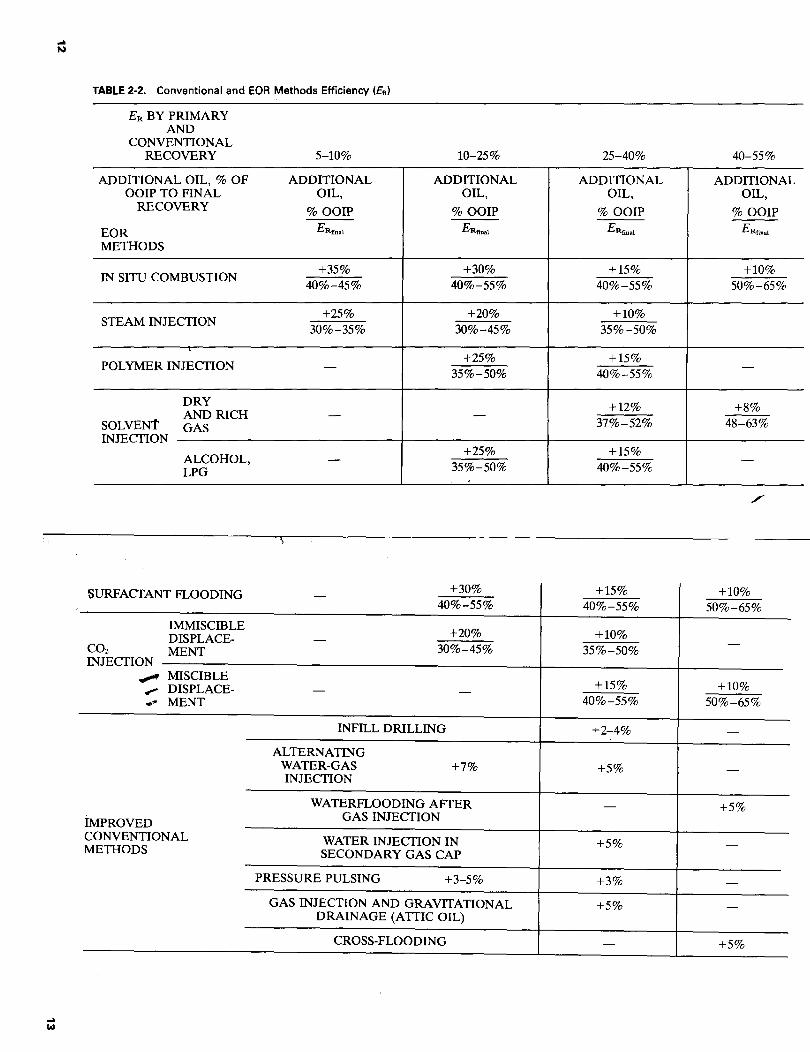
For instance, the ultimate oil recovery factor of individual reservoirs under primary and/or conventional recovery methods may range from 5 percent of OOIP for the poorest reservoir characteristics or for viscous oil, to as high as 55 or 60 percent of OOIP for the best reservoir characteristics or for light oil.
To achieve this desideratum the oil reservoirs are classified by several models according to the average of the ultimate oil recovery ERfin•l' expressed as a percentage of OOIP, possibly attained by the respective recovery mechanism, as follows:
£Rfinal
5-10% 10-25% 25-40%
40-55%
Tight oil reservoirs, slightly fractured or heavy oil reservoirs Oil reservoirs produced mainly by solution gas drive Oil reservoirs producing under partial water drive, gas injection, or gravity drainage Oil reservoirs produced by conventional waterflood
A possible estimation (Carcoana and Aldea, 1976) of the additional oil reserves, percentage of OOIP, that could be recovered as the result of EOR processes is shown in Table 2-2. These values can be safely used for a quick evaluation of the improved oil reserves and for the selection of methods that should be applied. For instance, for oil reservoirs where ER = 25-40 percent of OOIP obtained by primary or conventional methods, the implementation of the EOR methods would increase these values to 35-55 percent of OOIP. However, the selection of a certain process aimed at enhancing oil recovery must be made only after detailed investigations of the pertinent oil reservoir data (especially residual oil saturation), laboratory tests, and field pilots. The National Petroleum Council (NPC) study shows that the potential exists to add 11 billion bbl, approximately 40 percent of current proven reserves, to U.S. supply with existing EOR technology.
QUESTIONS AND EXERCISES
2-1 Define producing reserves by energy source criteria. 2-2 Show the target and path of EOR. 2-3 Explain why the ultimate recovery factor is different for different oil reservoirs. 2-4 Estimate the additional oil, expressed as a percentage of OOIP, possible to obtain
by steam injection and by surfactant flooding when applied to oil reservoirs developed by primary and conventional methods.
References 15
REFERENCES
CARCOANA,A., and GH. ALDEA, Marirea Factorulni Final de Recuperare Ia Zacamintele de Hidrocarburi (Bucharest, RO: Ed. Technica, 1976).
LA TIL, M., et a!., Enhanced Oil Recovery (Houston, TX: Gulf, 1980), p. 206. NATIONAL PETROLEUM COUNCIL, Enhanced Oil Recovery (Washington, D.C.: U.S.
Department of Energy, June 1984).
./

Chapter 3
Steam: A Heat Carrier Agent
Thermal recovery of oil using steam injected into the formation is similar to other hot fluid injection methods using water or gas. However, since steam is a better heat carrier, a higher oil displacement efficiency can be obtained with steam than with hot water or gas. For example, if water at 350 oF is injected into a reservoir with a 130 °F temperature, the heat content added to the reservoir is 224 Btu/Ibm. However, when steam at 350 oF is injected into a reservoir with a 130 °F temperature, the added heat content is 1194 Btu/Ibm. In addition to the higher heat content, the steam front's high temperature also generates other favorable effects such as vaporization and condensation. For these reasons steam has been preferred as an injection agent instead of hot water or gas.
3-1 LIQUID TO VAPOR PHASE CHANGE
Before steam is injected into the oil reservoir , it should be produced in the field using steam generators. We know how water is transformed into steam, but it
16
Sec. 3-1 Liquid to Vapor Phase Change 17
T;F
B
h 1000 psla 545
212 B
/A 14.7 psla
Volume Fig. 3-la Water to boiling point, B
is useful to consider some details regarding the liquid to vapor phase change (Bleakley, (a), 1965).
Boiling Point
By the application of heat, water gains internal energy, and the temperature increase can be illustrated as lineA-Bon a temperature-volume diagram (Figure 3-1a). When the boiling point B is reached, some liquid molecules have enough kinetic energy to escape through the liquid surface tension as vapor. At atmospheric conditions (14. 7 psia) the boiling temperature of water is 212 °F. At higher pressures the boiling temperature increases. For instance, at 1000 psia the boiling temperature of water increases to 545 °F. The amount of heat required to raise the water temperature until the boiling point B is reached (change in temperature without a phase change) is called sensible heat, Q. , and is expressed in British thermal units (Btu) or joules (J).
Q. = mc.:lT (3-1)
where
m = mass of water , lb or kg c = specific heat capacity, Btu/(lbm °F) or J/(kg oq (heat required to produce
a unit temperature change in a unit mass)
.:l T = 1! - To oF or oc
where 11 is the final temperature and To is the initial temperature of the mass m.
Vaporization Point
Continued application of heat causes the water to boil and vaporize at a constant~emperature and pressure (line B-V, Figure 3-lb). When vaporization
/

18 Chap. 3 Steam : A Heat Carrier Agent
545 8 v 1000 psla
212 8 v 14.7 psla
Volume
Fig. 3-lb Water and steam: the vaporization point , V
point V is reached all water in the liquid phase changes to vapor. The amount , of heat required to change the phase from liquid (water) to vapor (steam) at a constant temperature and pressure is called latent heat of vaporization, Q" (Btu or J),
(3-2)
where/" is the specific latent heat of vaporization (enthalpy of vaporization) and is expressed in units of Btu/Ibm or J/kg. Further addition of heat causes the temperature of steam to rise without an increase in pressure. This steam is said to be superheated.
Water-Steam Pressure-Volume Diagram
The line joining points B with different pressure values is called the bubble point line or saturated liquid line (Figure 3-lc).
When the liquid is saturated (one phase region) and heat is added, the temperature remains constant, the vaporization process begins and liquid
545
212
Critical point c
s
One phase: superheated steam
Saturated vapor line /
Volume
Fig. 3-lc Water-steam temperature-volume diagram
I (
Sec. 3-2 The Heat Content of Steam '-...
19
phase changes to vapor phase (vaporization line B-V, two phases). The line joining points V is called the dew point line or saturated vapor line. When the vapor is saturated and heat is added, the temperature increases (line V-S , one phase) and the steam is superheated. Inversely, when heat is taken from the superheated steam system, temperature decreases until point Vis reached on the saturated vapor line. If more heat is taken out , the temperature remains constant, vapor phase changes to liquid phase (condensation line V-B , two phases) until point B is attained, where all vapor is changed to liquid (one phase). Critical point C (3206.2 psia and 705.4 °F) is the point where the saturated liquid line and the saturated vapor line converge .
Each A-B-V-S line is also a constant-pressure line. The conversion of liquid water to steam occurs along a constant-pressure and constant-temperature line (line B-V). For a given temperature there is only one pressure at wltich water and steam can both be present. Field steam generators operate at constant pressure, higher than reservoir pressure, and in the two-phase region. The temperature of the output steam is also constant. In the two-phase region the steam temperature cannot be increased or decreased without respective increase or decrease in pressure. The two-phase region where both water and steam coexist is the area of importance in oil field steam operations.
3-2 THE HEAT CONTENT OF STEAM
The total amount of heat QT absorbed in the process of converting water into steam is given by
(3-3)
Steam Enthalpy
The amount of heat per unit of mass is called enthalpy, h , and is expressed in Btu/Ibm or J/kg. It is arbitrarily assumed that saturated water has a zero enthalpy value at 32 °F or 0 oc temperature and 0.08854 psia or 0.006 atmosphere (hoATUM = 0).
The amount of heat necessary for a mass unit of water at 32 oF and 0. 08854 psia to reach the boiling point B on the saturation liquid curve is given by the enthalpy of saturated liquid h1, Btu/Ibm or J/kg.
A Cartesian plot of the amount of heat (enthalpy) as a function of pressure is shown in Figure 3-2.
The total enthalpy h8 necessary to vaporize all liquid and to reach the point V on vaporization line is given by
(3-4)
wh~re h,8 .is the amount of absorbed heat needed to vaporize the water and is
20 Chap. 3
Presswe psi a
400
, 8. ~ / \ ~ "1:1 I \ "1:1 fiJB' , , V S ; 1,T=449.59'Ft, ; -,, ,, -IIIJ I I\ Ill en 1 1 1 , en
I I hfg = I \ I I btU I ~
1780.5,- 1
hf=424 hg=1204.5
Steam: A Heat Carrier Agent
Enthalpy, Btu lb
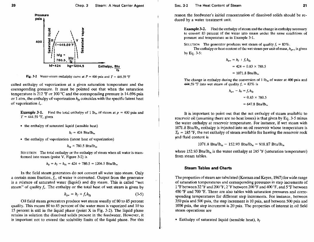
Fig. 3·2 Water-steam enthalphy curve at P = 400 psia and T = 449.59 op
called enthalpy of vaporization at a given saturation temperature and the corresponding pressure. It must be pointed out that when the saturation temperature is 212 oF or 100 oc and the corresponding pressure is 14.696 psia or 1 atm, the enthalpy of vaporization h1g coincides with the specific latent heat of vaporization lv.
Example 3-1. Find the total enthalpy of 1lbrn of steam at p = 400 psia and T = 444.59 °F, given
• the enthalpy of saturated liquid (sensible heat)
ht = 424 Btu/lbm
• the enthalpy of vaporization (latent heat of vaporization)
htg = 780.5 Btu/lbm
SOLUTION The total enthalpy or the enthalpy of steam when all water is transformed into steam (point V, Figure 3-2) is
hg = ht + htg = 424 + 780.5 = 1204.5 Btu/lbm
In the field steam generators do not convert all water into steam. Only a certain mass fraction, Is, of water is converted. Output from the generator is a mi~ture of saturated water (liquid) and dry steam. This is called "wet steam" of quality Is. The enthalpy or the total heat of wet steam is given by
(3-5)
Oil field steam generators produce wet steam usually of 80 to 85 percent quality. This means 80 to 85 percent of the water mass is vaporized and 10 to 15 percent is still in the liquid phase (point X in Fig. 3-2). The liquid phase retains in solution the dissolved solids present in the feedwater. However, it is important not to exceed the solubility limits of the liquid phase. For this
Sec. 3-2 The Heat Content of Steam 21
reason the feedwater's initial concentration of dissolved solids should be reduced by a water treatment unit.
Example 3-2. Find the enthalpy of steam and the change in enthalpy necessary to convert 83 percent of the water into steam under the same conditions of pressure and temperature as in Example 3-1.
SOLUTION The generator produces wet steam of quality f. = 83%. The enthalpy or heat content of the wet steam per unit of mass, hgw, is given
by Eq. 3-5:
hgw = h, + fshtg
= 424 + 0.83 X 780.5
= 1071.8 Btu/lbm
The change in enthalpy during the conversion of 1 lbm of water at 400 psia and 444.59 °F into wet steam of quality Is = 83% is
hgw - ht = /shfg
= 0.83 X 780.5
= 647.8 Btu/lbm
It is important to point out that the net enthalpy of steam available to reservoir oil (assuming there are no heat losses) is that given by Eq. 3-5 minus the water enthalpy at reservoir temperature. For instance, if wet steam with 1071.8 Btu/Ibm enthalpy is injected into an oil reservoir whose temperature is TR = 185 °F, the net enthalpy of steam available for heating the reservoir rock ~nd fluid content is
1071.8 Btu/Ibm- 152.93 Btu/Ibm= 918.87 Btu/Ibm
where 152.93 Btu/Ibm is the water enthalpy at 185 °F (saturation temperature) from steam tables.
Steam Tables and Charts
The properties of steam are tabulated (Keenan and Keyes, 1967) for wide range of saturation temperatures and corresponding pressures in step increments of 1 °F between 32 °F and 200 °F, 2 °F between 200 °F and 400 °F, and 5 °F between 400 oF and 700 °F. There are also tables with saturation pressures and corresponding temperatures for different step increments. For instance, between 350 psia and 500 psia, the step increment is 10 psia, and between 500 psia and 1000 psia, the step increment is 20 psia. The properties of interest in oil field steam operations are
• Enthalpy of saturated liquid (sensible heat), h1

22 Chap. 3 Steam: A Heat Carrier Agent
TABLE 3-1a. Properties of Steam
Abs. Enthalpy, Btu/Ibm
Temp. , Press., Specific Volume Saturated Change in Saturated (fe!lbm) of Saturated OF psi a Li~~id Enthalpy vcw.or
T p Liq. Vt Yap. vg htg g
425 325 .92 0.01902 1.4226 402.77 801.2 1203.5 430 343.72 0.01910 1.3499 407.79 796.0 1203.8 435 362.27 0.01918 1.2815 413.34 790.8 1204.1 440 381.59 0.01926 1.2171 418.90 785.4 1204.3 445 401.608 0.01935 1.1565 424.49 780.0 1204.5
• Enthalpy of saturated vapor (total heat), h8
• The change in enthalpy (latent heat), h18 = h8 - h1 • Specific volume of saturated liquid, v1, ft3/lbm • Specific volume of saturated vapor, v8 , ft3/lbm
Tables 3-la and 3-lb show enthalpy and specific volume values of water and steam at saturation temperatures from 425 to 445 °F (Table 3-la) and at saturation pressures between 400 and 440 psia (Table 3-lb).
The enthalpies and specific volumes of saturated water and saturated steam at different pressures and temperatures can also be found from charts especially prepared. Figure 3-3 is a pressure-enthalpy chart for steam.
Figure 3-4 represents the variation of sensible (hv), latent (h18 ), and total heat of steam (h8 ) with pressure. It is interesting to observe that , starting at approximately 470 psia, the total heat of steam decreases with an increase in pressure. The reason for this can be understood by observing how the twophase area (latent heat) is reduced when the saturated vapor line and saturated lfquid line converge at the critical point (Fig. 3-4). The decrease in the latent heat content of steam becomes larger than the increase of the sensible heat with pressure .
TABLE 3-1b.
Abs. Press., Temp.,
psi a OF p T
400 444.59 0.0193 1.1613 424.0 780.5 1204.5 410 447.01 0.0194 1.1330 426.8 777.7 1204.5 420 449.39 0.0194 1.1061 429.4 775 .2 1204.6 430 451.73 0.0194 1.0803 432.1 772.5 1204.6 440 454.02 0.0195 1.0556 434.6 770.0 1204.6
Abridged tables are from Joseph H . Keenan and Frederick G . Keyes, Thermodynamic Properties of Steam, thirty-ninth printing (New York: John Wiley & Sons, © 1967), pp. 32, 38.
Sec. 3-2 The Heat Content of Steam
Press we pala
3000 I I Crltlc~~lnt I I
3206.2 puV.7J -- ~o5.4"F-J 1\
~-V-- v60( "F·· ---\ / --J. 55~1 F,_ c
0
2000
1000 800 700 600 500 400
Liquid Region t500 "F-1-· Cl ----- CD
300
200
100 80
0 200
a: ~/ /1 lT ... J.j- ~ ~-y4~0 "F >.-'-;; 1-· ---~
&. -...1 ~ ~ ...... ~ bt,...__. ~ :::: = - ~ CD a 1f T CD t8 ~ ~- -J •oo, a-a ., ... -: ~ 1. ~ ~ 1- CD -,: tit C) :g C) ;
---- --'SL 35o ·FfL~ _!!J
I I I I I ; en
Two /PhasejReglo?f- ·
400 600 800 1000 1200
ENTHALPY,Btu/lb
Fig. 3-3 Pressure-enthalpy chart for steam (From Bleakley, 1965)
23
In other words, if the steam's injection pressure is just enough to displace the reservoir fluids , it will have more heat content than at higher pressures.
Steam Quality
Figure 3-3 also shows steam quality lines or lines connecting the points' with the same steam quality values. Steam quality can be determined by different methods such as the separator method, conductivity-meter method , chloride method, and the orifice-meter measurement (Bleakley, (c), 1965).
~ 1000 -::I .... ID BOO ...: z w 600 .... z 8 400
~ w 200 :J:
0..___._____._~-~----'----'-....l
0 500 1000 1500 2000 2500 3000 ABSOLUTE PRESSURE, PSIA
Fig. 3-4 Variation of sensible , latent , and total heat of steam with pressure (From Farouq Ali , 1970)

24 Chap.3 Steam: A Heat Carrier Agent
Saturation Method. The mass rates of the liquid phase and of the dry steam separated in an insulated vessel are measured under pressure over a short period of time. The steam quality is given by the ratio mass rate of vapor flow to mass rate of flow of the vapor and liquid steam.
Conductivity-Meter Method. This method is based on the resistance to flow of electrical current. More salt dissolved leads to less resistance to flow, which leads to higher electrical conductivity. Steam quality can be calculated by measuring the electrical conductivity of the feedwater and liquid phase of the wet steam. For instance, if the conductivity of the liquid phase of steam is six times higher than that of the feed water, five-sixths of the feedwater has been vaporized and the steam quality is~= 0.833.
Chloride Method. The chloride method measures only the chloride ion, C1, contained in both stream flows instead of measuring the conductivity resulting from the total salt content.
11 Orifice-Meter Method. This method measuring superheated and highquality steam flow rates has been adapted by Pryor (1966), to determine quality x of wet steam used in injection steam operations:
X= (c~rl (3-6)
where
W = flow rate of wet steam, gallons per minute (gpm), is determined by measuring the inlet water using an orifice meter, since oil field generators are designed for steady flow
C = combination of flow constant for the size of pipe, orifice diameters, and orifice plate expansion; units conversion is given for average conditions in tables such as Table 3-2 (abridged)
TABLE 3-2. C, Constant Values (bellows type, W.C. meter)
Orifice plate
2.125 2.000 1.875 1.750 1.625 1.500
2.626-in. ID meter run (Win gpm)
100 in.
2.640 2.196 1.844 1.524 1.272 1.048
200 in.
3.720 3.092 2.600 2.148 1.796 1.480
400 in.
5.280 4.392 3.688 3.048 2.544 2.096
TABLE 3.2. (continued)
3.068-in. ID meter run (Win gpm)
Orifice plate 100 in. 200 in.
2.375 3.144 4.44 2.250 2.692 3.80 2.125 2.312 3.260 2.000 1.980 2.788 1.875 1.688 2.380 1.750 1.424 2.004 1.625 1.208 1.704 1.500 1.016 1.432 1.375 0.844 1.192 1.250 0.692 0.976
3.438-in. ID meter run (Win gpm)
Orifice plate 100 in. 200 in.
2.750 4.380 6.20 2.625 3.820 5.40 2.500 3.320 4.692 2.375 2.872 4.060 2.250 2.504 3.544 2.125 2.192 3.100 2.000 1.892 2.672 1.875 1.624 2.300 1.750 1.400 1.980 1.625 1.192 1.684 1.500 1.000 1.416 1.375 0.836 1.180 1.250 0.688 0.972 1.125 0.556 0.784 1.000 0.436 0.616
4.026-in. ID meter run (Win gpm)
Orifice plate 100 in. 200 in.
3.000 4.84 6.86 2.875 4.32 6.116 2.750 3.828 5.42 2.625 3.40 4.808 2.500 3.008 4.26
From Pryor (1966).
400 in.
6.288 5.384 4.624 3.960 3.376 2.848 2.416 2.032 1.688 1.384
400 in.
8.76 7.64 6.64 5.74 5.008 4.384 3.784 3.248 2.80 2.384 2.00 1.668 1.376 1.108 0.872
400 in.
9.68 8.64 7.652 6.80 6.012
25

26 Chap.3 Steam: A Heat Carrier Agent
h = differential pressure across the orifice in inches of water (from recorder) wd = density of the dry saturated steam determined from steam tables, lbm/ft
3
Example 3-3. Calculate the wet-steam quality of a ~50 m3/day .feed~ater steam generator working at 1000 psia saturation pressure gtven a 2. 75-m.-dtameter orifice plate in 4.026-in. ID meter run and 100 in. W.C. bellows meter recorder.
SoLUTION From recorder
vh = 3.8 or 28.9 in. of water
From steam tables
1 3
wd = 0.4456 lbm/ft the density of saturated vapor at 1000 psia
From Table 3-2
where
c = 3.828
xz = 3·828V2.244 x 3·8 = 0.89 or 89.0% 27.5
1 bbl 1 150 m3/d x 0. 159 m3 x 42 gallbbl x 24 x 60 min/day= 27.5 gpm
3-3 WET-STEAM GENERATORS
In the field the steam needed for injecting through wells in the oil reservoir is produced by wet-steam generators. Field steam generators are oi~- or gas-fired units designed for automatic operation, with forced and contmuous water circulation. Air pollution regulations are very strict regarding the control of emissions from oil-fired generators, especially when the fuel used to fire the
/ generator contains sulphur. . . . A wet-steam generator is aqua tubular, havmg water-filled tubes wtth the
flame and hot gases surrounding the tubes. The tubes can be coil shaped, and water is pumped through them at high velocity and turbulence, contrary to the flow direction of the hot gases as shown in Figure 3-5a. The water-filled tubes can also be straight, running back and forth along the length of the generator. In this case the unit has an economizer to preheat the water (Figure 3-5b ). A comparison between these two types of generators is shown in Table 3-3.
Steam generators are furnished as mobile units on a skid, trailer mounted (truck mounted), or as permanent installations on a pad. The recomme~ded practice for installation and operation of wet-steam generators was estabhshed by the American Petroleum Institute (API, 1983).
Wet-steam generators are usually rated in millions of Btus per hour of
Sec. 3-3 Wet-Steam Generators
Control
0
Fig. 3-Sa Steam generator with coil-shaped water filled tubes
Fig. 3-Sb Steam generator with straight water-filled tubes
Steam Output
Water Input
27
heat absorbed. Those used in enhanced oil recovery range from 12- to 50-MM Btu/hr steam output. They can produce steam with a saturation pressure of up to 200~2500 psia and a quality frequently between 80 and 85 percent. The steam saturation temperature corresponds to the respective saturation pressure.
Example 3.4. Find the capacity in tons of steam per hour and the saturation temperature of a 24-MM Btu/hr wet-steam generator operating at 1560 psia saturation pressure and producing steam with f, = 80% quality.
SOLUTION Using the steam tables we find that the given condition of 1560 psia saturation pressure is not listed. The problem requires interpolation between 1500 and 1600 psia values. At a saturation pressure of 1560 psia (105 atm), the heat content of the wet steam
hgw = hf + f, hfg = 619.1 + 0.8 (543.3)
= 1053.7 Btu/Ibm

28 Chap.3 Steam: A Heat Carrier Agent
TABLE 3-3. Steam Generator Water-Filled Tubes Comparison
Water-Filled Tubes
Advantages
Disadvantages
Coil
Requires no preheated water. Reduced refractory surface
and better portability. Coils easily cleaned by acid
solution circulation and rinsing.
Higher temperature per unit of heated area and more chances of damages.
Difficult repair work for the first row (external) of coils.
Straight
Strongly built and fewer chances of damages.
Easier replacement of the straight tubes.
More refractory material. Heavier. Elbow shock loads at both ends
of the straight tubes. Hot gas carbon deposits over
the economizer tubes.
If a 1-lb mass of steam at 1560 psia saturation pressure has 1053.7 Btu, then 1000 kg or 1 ton of steam has
1000 kg X 1053.7 Btu/lbm = 2 323 1
.n6 B 0.4536 kg/Ibm · X u tu
and
24 X 106 Btu/hr 24MM Btu/hr = 2.323 x 10⁶ Btu/ton = 10.33 tons/hr of steam
at 1560 psia saturation pressure and 601.43 op saturation temperature. A rough but faster estimation can be made using the pressure enthalpy chart for steam (Figure 3-3) to read the water and steam enthalpy values at 1560 psia.
3-4 FEEDWATER TREATMENT
The water used in the field to feed a wet-steam generator should be of good quality to avoid scaling, tube corrosion, and suspended solids in the effluent. The American Petroleum Institute (API-RP, 1983) recommends that the following factors be considered in the treatment of feedwater:
Total hardness Iron concentration Total dissolved
solids (TDS)
Less than one part per million (ppm). Less than 0.1 ppm. "Levels of TDS become a cause of concern only when liquid phase concentrations approach solu-
Sec. 3-5 Heat Losses
Suspended solids Suspended oil content Oxygen Alkalinity
Silica
pH
29
bility. Therefore a unit producing 80% quality steam should be able to tolerate feedwater dis-t solved solids in concentrations approaching 20 percent of their solubility limits." Below 5 ppm and preferably below 1 ppm. Below 1 ppm. Less than 0.01 ppm and preferably 0.0 ppm. Moderate alkalinity levels help reduce corrosion and maintain silica solubility. Bicarbonate alkalinity levels of over 2000 ppm should be avoided. Control consists of maintaining solubility which is strongly affected by alkalinity. Alkalinity should be maintained at a level at least three times that of the silica content. From 7 to 12.
Different types of steam generators are provided with water treatment units. To avoid high maintenance costs and low generator efficiency, the source and chemical composition of the water must be analyzed and the water treatment unit must be adjusted to the specific conditions determined by the analysis.
3-5 HEAT LOSSES
The steam generated by a wet-steam generator is the heat carrier agent injected into the reservoir. It raises the temperature of the rock and fluids it contains and displaces the oil. Not all the heat carried by the steam reaches the reservoir fluid and stays in the reservoir. Some of the heat is lost at the surface some is lost into the wellbore, and some is lost to the adjacent formations. H~at can be transmitted away by conduction, convection, radiation, or combinations of all three means. Also, part of the heat reaching the reservoir is lost through produced fluids. Detailed information regarding the heat loss calculations and heat transmission were presented by Ramey (1962), Pacheco and Farouq Ali (1972), Prats (1982), and White and Moss (1983), among others.
The amount of formation heated depends on the amount of heat lost
• in the steam generator • on the surface transmission lines • from the wellbore • to adjacent formations

30 Chap.3 Steam: A Heat Carrier Agent
Steam Generator Heat Loss
The heat lost in the steam generator, Qg, is given by a material balance between the heat released through the fuel-burning process and the heat gained by steam. The total heat, Q, liberated by the direct combustion of fuel is
Q=Hm (3-7)
where His the heat of combustion or the heat evolved when a unit mass m (or volume) of fuel is completely burned, Btu/lbm or J/kg. The total heat absorbed or the enthalpy, hgw, of wet steam is given by Eq. 3-5 minus the enthalpy of the feedwater. Therefore, the steam generator heat loss is
(3-8)
Example 3-5. A steam generator produces steam of 85 percent quality at 1000 psia saturation pressure, consuming 911lbm/hr fuel oil with 19,800 Btu/Ibm heat of combustion. The feedwater rate is 150m3/day at 60 °F. Find the heat loss and the efficiency of the generator.
SOLUTION Total heat produced is
Q = 19,800 Btu/Ibm X 91llbmlhr = 18.04 X 10⁶ Btulhr
Wet-steam enthalpy at 1000 psia saturation pressure (from steam tables) is
hgw = hr + f,hfg = 542.4 + 0.85(649.4) = 1094.4 Btu/Ibm
The change in enthalpy from water to wet steam is
1094.4 Btu/Ibm - 28.06 Btu/Ibm = 1066.34 Btu/Ibm
where 28.06 Btu/Ibm is hteedw or the enthalpy of feedwater at 60 oF saturation temperature (steam tables).
Total heat gained by steam is
1 day 150 m3/day x 1000 kg/m3
X 2.204 Ibm/kg X 24
hr X 1066.34
Btu/Ibm = 14.689 X 10⁶ Btulhr
The heat lost is
Q8 = (18.04 - 14.689) x 106 = 3.35 x 10⁶ Btu/hr or 18.6%
and is mostly due to flue gas emissions. The generator efficiency is
( 3.35 X 10⁶
) E = 1 - 18.04 X 106 X 100 = 81.4%
Sec. 3-5 Heat Losses -.!-31
Heat Loss on the Surface Transmission Lines
The surface transmission lines conduct steam from the generator to the wellhead and into the wellbore. The heat lost, Q,, by conduction and radiation on surface lines is
(3-9)
where
A = the surface area of steam pipelines, ft2 Uo = overall heattransfer coefficient, Btu/hr x ft2 X op (an average of various
transfer coefficients of all the exposed surfaces that make up the steam transmission lines)
~T = ~.,- T.x,, temperature difference, op
The heat losses are minimized to 3 to 5 percent if the surface steam pipelines are insulated or buried and are higher if lines are bare and/or the climate is cold.
Heat Loss from the Wellbore
Wellbore heat loss is a factor seriously limiting the use of steam injection to shallow wells. As the wet steam flows through tubing down the wellbore to the reservoir, the tubing is heated to the steam temperature. The tubing loses heat with time by transferring it through the annulus to the casing and through the cement behind the casing to the ground. The problem of heat transmission in the wellbore is complex, and since it is also important, a number of author&" have treated it in detail. Ramey (1962) considered the geothermal gradient and radiation conditions, and Willhite (1967) explained the overall heat transfer coefficient in steam injection. More recently Pacheco and Farouq Ali (1972) and Farouq Ali (1981) improved a mathematical model for wellbore steam injection under various flow regimes. Also, White and Moss (1983) published details of heat transfer in the wellbore and examples of the calculation procedures.
Figure 3-6 shows wellbore heat loss as a function of injection rate. As we observe, increasing the injection rate causes the steam pressure to
decline due to higher friction along the tubing string. Correspondingly, at a lower saturation pressure, there is a lower temperature and more hot liquid will vaporize. The steam quality increases and the heat loss as a percentage of total heat can be reduced.

32 Chap.3 Steam: A Heat Carrier Agent
c: Q) u ... Q)
a..
80 600
60 500
40 400
20 300
oL-----L--L--~~--~~--~~--._-*200 2000 4000 6000 8000 10000
Injection Rate, Lb/Hr
Tubing O.D. -2-3/8" Depth - 1 000' (10,000 Lb/Hr = 686 BSPD)
INJ. Press- 500 Psia Time - 10 Days
"' ·;;; a.. Q) ... ::I
~ Q)
ct
Fig. 3-6 Wellbore heat Joss as a function of injection rate (From Pacheco and Farouq Ali, 1972)
For a given steam injection rate, field methods to reduce heat loss from the wellbore (Farouq Ali and Meldau, 1983) include
• insulated tubing • casing-tubing annulus vented to the atmosphere • concentric tubing strings with insulating material between • crude oil gel placed in the annulus • high-pressure gas pack in the annulus
All these methods increase the resistance to heat flow from the wellbore. The effect of reducing the heat loss from the wellbore is illustrated in Figure 3-7. The heat lost in the wellbore ranges from 5 percent of total heat input, if it is well insulated, to 25 percent without insulation. The comparison is made for the working conditions listed in Figure 3-7.
The total heat loss from the wellbore when steam is injected down tubing
Sec. 3-5 Heat Losses
No Insulation
i1: Gas Pack -: a. ~ Vented Annulus ::!: u; UJ ... !/)
0 C) ...1 z < Crude 011 Gel ti u;
c( UJ 0 J: < Solid Insulation
DEPTH 2000' PRESSURE 1000 pslg RATE 500 BSPD
TIME 30 DAYS TUBING 2-7/8"
CASING 7"
Fig. 3-7 Insulated tubing heat loss comparison (From Farouq Ali and Meldau, 1983)
33
can be estimated in the field using Ramey's (1965) equation for the heat loss rate Qw, Btu/day:
Q = 2Tir1 Uk [(T _ b )Z _ aZ2]
w k + r1 Uf(t0 ) a 2 (3-10)
where
r1 = inside tubing radius, ft "'
U = overall heat transfer coefficient between inside of tubing and outside of casing, Btu/day x ft2 x °F, and where area is based on r 1
k = thermal conductivity of the earth, Btu/day X ft x oF f(t0 ) = dimensionless transient heat conduction time function
I'a = saturation temperature of steam ~t prevailing pressure, °F b = surface geothermal temperature, °F Z = formation depth, ft a = geothermal gradient, °F/ft
Under the particular conditions listed in Table 3-4, Ramey obtained the heat loss rate values after 100 days' steam injection time.
For different casing sizes and injection times, and assuming that the thermal diffusivity of earth is a constant = 0.96 ft2/day, the dimensionless transient heat conduction time function f(tv) values are given in Table 3-5.

34 Chap.3 Steam: A Heat Carrier Agent
TABLE 3-4. Estimated Wellbore Heat Loss Rate for Steam Injection at 100 Days' Injection Time
Conditions: Geothermal gradient, a = 0.02 °F/ft Geothermal surface temperature = 70 oF Overall heat-transfer coefficient, u = 30 Btu/day X te X OF Tubing size == 2 in.; r1 == f2 Casing size = 7 in. Thermal conductivity of earth, k = 33.6 Btu/day X ft X oF Thermal diffusivity of earth == 0.96 ft2/day
Heat Loss Rate, MM Btu/day for steam temperature at
Formation depth, ft 300 °F 400 °F 500 °F 600 °F
500 1.36 1000 2.67 1500 3.91 2000 5.08 2500 6.21 3000 7.28
Source: Ramey (1965).
1.97 3.88 5.72 7.50 9.25
10.90
2.57 5.10 7.55 9.92
12.26 14.54
3.18 6.30 9.36
12.32 15.30 18.19
Example 3-6. Calculate the percentage of heat loss in a well-insulated wellbore when the wet steam produced by a generator (Example 3-5) reaches the wellhead and is injected through 3-in. tubing to a 2000-ft depth. The wellbore conditions are those outlined by Ramey in Table 3-5, and the injection time is 100 days.
SOLUTION The wet-steam temperature is 544.61 oF when saturation pressure is 1000 psi a (steam tables). The dimensionless functionf(tv) for 7 -in. casing size and WO days' injection time is 3.98 (Table 3-5).
TABLE 3-5. Values of f(t0 ) for Different Casing Sizes and Injection Time
Days Casing
Size, in. 5 25 50 75 100
4~ 2.96 3.81 4.08 4.37 4.48 5~ 2.89 3.56 3.99 4.08 4.27 7 2.64 3.32 3.64 3.90 3.98 8~ 2.46 3.10 3.42 3.64 3.81
From Bleakley (1965).
..
Sec. 3-5 Heat Losses 35
The heat loss rate is
2'11' 1.~ i~f (30 Btu/day x frZ x °F)(33.6 Btu/day x ft x °F) Q = 12 Ill. t
w 10 (33.6 Btu/day x ft x °F) + l
2 ft(30 Btu/day x ft2 x °F)3.98
X [ (544.61 - 70) °F X 2000 ft - 0.02 2oF/f\2000)2 ft2]
= 527
·78
(949 220- 40 000) == 11.02 X 10⁶ Btu/da 43.550 , ' y
or 459,116 Btu/hr. This represents 3.12 percent heat lost from the total heat gained by the steam (14.689 x 10⁶ Btu/hr, Example 3-5). The heat loss can increase four to five times, and mechanical problems may occur if the wellbore completion is not provided with insulation.
Downhole Steam Generator
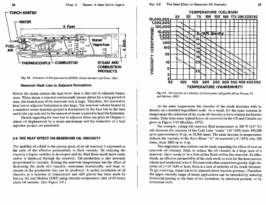
The failure conditions to which tubular goods are subjected in steam injection wells and excessive heat losses can be avoided by generating the steam downhole. Mechanical problems and heat losses were the main incentives for developing a downhole steam generator. Schrimer and Eson (1985), among others, investigated the concept of using a direct-fired downhole steam generator (DFDSG) in steam injection operations.
In this type of generator, fuel and air are injected separately into the wellbore reaching a downhole combustion chamber placed in front of the productive formation. After the fuel is ignited with an electrical torch igniter, water injected into the combustion chamber comes in contact with the burner flame and vaporizes into steam (Figure 3-8).
Use of both fuel and air transported continuously downhole to the steam generator creates safety problems not experienced in conventional surface steam generators. The hazards that should be avoided are the leakage of fuel (gas) or air and the mixture conditions favorable to explosion in the wellbore.
The main advantages over conventional steaming methods are described as
• reduction in heat losses • reduction in air pollution • deeper steaming potential • offshore potential (smaller-size facilities and use of sea water) • reservoir pressurization (higher pressure for steam drive around the well)
36
TORCH IGNITER
\WATER
\ ,. q
~·0-lllioiiU;..l<'S~ ....
FUEL
AIR ~ ---~ ~
LTHERMOCOUPLE
Chap.3
6 Feet
COMBUSTOR
Steam: A Heat Carrier Agent
STEAM AND COMBUSTION PRODUCTS
Fig. 3-8 Schematic of flow patterns for DFDSG (From Schrimer and Eson, 1985)
Reservoir Heat Loss to Adjacent Formations
Before the steam reaches the heat front, heat is also lost to adjacent formations. When steam is injected continuously (steam drive) for a long period of time, the heated area of the reservoir rock is large. Therefore, the cumulative heat loss to adjacent formations is also large. The reservoir volume heated by a sustained steam injection project is determined by the heat lost to the base and to the cap rock and by the amount of steam required to heat the formation.
Details regarding the heat lost to adjacent strata are given in Chapter 4, where oil displacement by a steam mechanism and the evaluation of a heat injection project are presented.
3-6 THE HEAT EFFECT ON RESERVOIR OIL VISCOSITY
The mobility of a fluid in the porous space of an oil reservoir is expressed as the ratio of the effective permeability to fluid viscosity. By reducing the viscosity a higher mobility is developed and the fluid flows much more easily and/or is displaced through the reservoir. Oil production is also inversely proportional to viscosity. Raising the reservoir temperature has the effect of decreasing the crude oil's viscosity, sometimes dramatically, and large increases in the production rate can be predicted. A useful correlation of oil viscosity as a function of temperature and API gravity has been made by Farouq Ali and Meldau (1983) using viscosity-temperature data of 60 heavy crude oil samples. (See Figure 3-9.)
Sec. 3-6 The Heat Effect on Reservoir Oil Viscosity
10,000,000 1,000,000 - 100,000 UJ S!! 10,000 0 3,000 2: 1,000 ~ 300 w 100 0 -> !:: en 0 0 en >
30
10
5
3
TEMPERATURE (CELSIUS) 25 50 75 100 125' 150 175 200225250
""' "-
""' ' i'.... ............ a-·A I' I ~ravl tv ~ ' ' ~"'.:
-;~'--... ~ ~ 10 r-... ..........
I'.. I'.. ['-.. 12 I'- ...... ........ ~
"" "" .......... 14
r-..... I'. ........
' ...........
~ 16 ....... ~ ....... 18 [":: ......
' ' r---.. r-... ~ "" 20 ~ ' ' ~ ......... r--..
I". r-..... .......... ......
' ........... r-... r--..
""' ......... ' ' r-... ~ r....... t"..... ·, 25 '· ' ~"- .... f-.. ~ !"". .... ., ~ ....... ~
.....
37
2 50 100 150 200 250 300 350 400 450500
TEMPERATURE (FAHRENHEIT)
Fig. 3-9 Oil viscosity as a function of temperature and gravity (From Farouq Ali and Meldau, 1983)
At the same temperature the viscosity of the crude increases with its density on a doubled logarithmic scale. As a result, for the same increase in temperature the reduction of the crude oil viscosity is more evident for heavier crudes. Data from some typical heavy oil reservoirs in the US and Canada are given in Figure 3-10 (Buckles, 1979).
For example, raising the reservoir fluid temperature to 300 °F (147 oq will decrease the viscosity of the Cold Lake "crude" (10 °API) from 100,000 cp to approximately 10 cp, or 10,000 times. The same increase in temperature reduces the viscosity of the Kern River "A" oil reservoir (14 °API) only 500 times, from 2000 cp to 4 cp.
Two important observations can be made regarding the effect of heat on reservoir oil viscosity. First, to reduce the oil viscosity in a large area of a reservoir, there needs to be a flow of hot fluids within the reservoir. In other words, an effective permeability of the rock needs to exist for the heat carriers (steam and condensed water). For reservoirs that contain low-gravity, high-viscosity oil ( = 10 o API or less), there is a lack of mobility of the crude bitumen. To get it moving, steam has to be injected above fracture pressure. Therefore the upper viscosity range of steam applications can be extended by inducing horizontal parting at the base of the formation, by electrical preheat, or by horizontal wells.

38
10,000,000 1,000,000
100,000
!II 10,000
0 1,000 11. i= z w () I > ... iii 0 ~ s:
100
10
3.0
Chap. 3 Steam: A Heat Carrier Agent
TEMPERATURE, °C 50 100 150 200 250
Q,j. _l _l ........ _l I
tl"'-"" ~Athabasca -Reservoir ~ Conditions
' 2' ~ t<' Jobo II
Uoyd.J.Inster ~[)~~ Pilon !'..: ~ !/'Cold La,ke
t•rn
1
River·/ ""' 1-
i'.
~R·r·tj 100 200 300 400 500
TEMPERATURE,'F
Fig. 3-10 Typica heavy oil viscosity-temperature relationships (From Buckles, 1979)
The second observation is that reduction of the crude oil's viscosity is the main but not the only recovery mechanism developed in the reservoir by steam injection. There are several other displacement mechanisms that occur such as steam vapor drive, distillation of the lighter fractions, and thermal expansion of the oil. Therefore steam injection may also be applied to reservoirs with medium or light crude oils to which these effects are prevailing.
QUESTIONS AND EXERCISES
3-1 Explain the water-steam (temperature-volume) phase diagram.
3-2 What is the main characteristic of the two-phase region on a steam pressureenthalpy diagram?
3-3 Is it possible to increase the temperature of steam coming from a generator and still operate at about the same steam quality? If so, how is it possible?
3-4 A mass of 5000 lbm of water has to be vaporized at 212 oF saturation temperature. Find (a) the sensible heat content (the enthalpy of saturated liquid) (b) the total heat content after vaporization (c) the change in enthalpy (d) the saturation pressure
3-5 How much heat (in joules and Btu) is produced when 1000 Ibm of steam are condensed at 150°C?
3-6 What is the amount of heat per hour required to generate steam of 82 percent quality at 860 psia if the 70 m3/day feedwater temperature is 45 oF?
References 39
3-7 Find the wet-steam quality of a 75m3/day feedwater steam generator working at 420 psia saturation pressure, given 2.5-in. orifice plate in 3.438-in. meter run and 400-in. W.C. bellows meter recorder; the meter reading is 1.6 (5.12 in. of water).
3-8 A 50-MM Btu/hr steam generator operates at 400 psia saturation pressure and produces steam with 82 percent quality. Find the capacity of stream in tons per hour and the saturation temperature of the steam.
3-9 Find the efficiency of a steam generator and the heat loss when the working conditions are
Waterfeed rate Saturation temperature Waterfeed temperature Wet-steam quality Fuel heat of combustion Fuel consumed
140m3/day 445 °F
70 °F 84%
19,800 Btu/Ibm 890 lbm/hr
3-10 Calculate, after 100 days' injection time, the amount of heat transported by wet steam of 83 percent quality injected through 2!-in. tubing and reaching the production formation at a depth of 1400 feet. Assume a wet-steam saturation temperature of 430 oF and the wellbore conditions given in Table 3-5. The waterfeed rate is 550 bbl/day at 60 °F. Assume the heat loss from surface transmission lines is 5 percent of the heat gained by steam in the generator.
REFERENCES
API, Recommended Practice for Installation and Operation of Wet Steam Generators (Dallas, TX: American Petroleum Institute, Production Department, March 1983).
API, Recommended Practice-Wet Steam Generator Feed Water Quality, Appendix A, 26 (Dallas, TX: American Petroleum Institute, 1983).
BLEAKLEY, W. B., "The How and Why of Steam," Parts 1 and 2, Oil and Gas Journal (January 11 and 18, 1965), pp. 75, 102. (a)
BLEAKLEY, W. B., "Finding Enthalpy and Specific Volume from Charts," Part 5, Oil and Gas Journal (February 15, 1965), p. 121. (b)
BLEAKLEY, W. B., "How to Find Steam Quality," Part 7, Oil and Gas Journal (March 1 and 8, 1965), pp. 76-77. (c)
BUCKLES, R. S., "Steam Stimulation Heavy Oil Recovery at Cold Lake Alberta," SPE 7994 presented at the 49th California Regional Meeting, Ventura, California, April 18-20, 1979.
FAROUQ Au, S.M., Oil Recovery by Steam Injection (Bradford, PA: Producers, 1970). FAROUQ Au, S.M., "A Comprehensive Well-bore Steam-Water Flow Model for Steam
Injection and Geothermal Applications," Society of Petroleum Engineering Journal (October 1981).
FAROUQ Au, S.M., and R. F. MELDAU, "Steam Flooding," Chapter VII in Improved Oil Recovery (Oklahoma City, OK: Interstate Oil Compact Commission, March 1983), pp. 314, 324, 339.
40 Chap. 3 Steam: A Heat Carrier Agent
KEENAN, J .. and F. KEYES, Thermodynamic Properties of Steam (New York: John Wiley & Sons, 1967), pp. 32, 38.
PACHECO, E. F., and S.M. FAROUQ ALI, "Well-Bore Heat Losses and Pressure Drop in Steam Injection," Journal of Petroleum Technology (February 1972).
PRATS, M., Thermal Recovery, SPE Monograph Series (New York, Dallas: American Institute of Mining, Metallurgical and Petroleum Engineers, 1982).
PRYOR, J. A., "Orifice Meter Measures Steam Quality," Oil and Gas Journal (May 30,
1966), p. 86. RAMEY, H. J., JR., "Well-bore Heat Transmission," Petroleum Transactions (AIME,
1962), pp. 225, 427. RAMEY, H. J., JR., "How to Calculate Heat Transmission in Hot Fluid Injection,"
in Fundamentals of Thermal Oil Recovery (Dallas, TX: Petroleum Engineer., 1965),
p. 165. SCHRIMER, R. M .. and R. L. EsoN, "A Direct-Fired Downhole Steam Generator-From
Design to Field Test," Transactions of the SPE, Vol. 279 (1985). WILLHITE, G. P., "Overall Heat Transfer Coefficients in Steam Injection and Hot Water
Wells," Journal of Petroleum Technology (May 1967), pp. 607--615. WHITE, P. D., and J. T. Moss, Thermal Recovery Methods (Thlsa, Oklahoma: Penn Well,
1983), Chapter 6.
Chapter 4
Steam Injection
4-1 GENERAL
Steam injection is the thermal process which supplies the heat needed to increase reservoir temperature and the energy to displace oil. Steam is the heat carrier agent provided by the steam generator. Continuous steam injection is called steam drive. Steam drive uses a pattern flood with injector and producers. In a single well operation, injecting steam and then producing oil from the same well, steam injection is called cyclic steam injection, steam soak, or "huff-and-puff."
The main purpose of steam drive is to increase the ultimate recovery factor. Cyclic steam injection's principal effect is to stimulate the formation to produce at a higher rate. Only when specific reservoir characteristics are present (shallow oil reservoirs with high dip and high lateral permeability) does cyclic steam injection stimulate gravity and drainage effect and increase the recovery factor through interwell communication.
The first report of a continuous steam injection field experiment was published in 1934 by Stovall. The Woodson-Texas field test was performed in an inverted nine-spot pilot by injecting steam at 200 psia pressure for 235 days
41

42 Chap.4 Steam Injection
in a formation 18 ft thick at a depth of 380 ft. The production rate of the wells around the injection well increased eight times.
Cyclic steam injection was implemented in the United States in 1933 and 1936. After a gap of 25 years this method resumed and developed, especially in California. The partially depleted California oil reservoirs (with depths of less than 3000 ft, a thickness between 40 and 300ft, and still high oil saturations) have been appropriate candidates for steam injection. The number of cyclic steam injection operations increased from 4 in 1962 to 111 in 1964 and to more than 420 in 1967. This "boom" in the use of cyclic steam injection can be credited to the method's immediate effect of increasing wells' oil production rates and to the availability of high-performance steam generators. Efficiency was increased by an average of 200 bbl/day additional oil produced by each steam generator in operation.
Commercial application of steam processes has been underway since the early 1960s, and the wealth of field experience with respect to their use makes them the most advanced of all EOR methods.
4-2 PROCESSES DESCRIPTION AND RECOVERY MECHANISMS
The steam injected into the reservoir transmits heat to the formation and the fluids it contains. The heat lowers the oil's viscosity and increases its mobility. As steam cools, it condenses into water. In a steam drive process, as steam is continually injected into the injection wells, the condensed water is pushed further through the reservoir to the producing wells. In a cyclic steam injection process, the condensed water is produced along with the oil stream by the same producing well.
Steam Drive Process
A cross section of a steam injection well and a producer in a reservoir formation with uniform permeability is shown in Figure 4-1.
As we observe, because of density differences, the steam segregates gravitationally and overrides. This tendency favors the early breakthrough of steam into the producers. As a consequence, only the upper one-third of the reservoir is swept by steam. To reduce the override tendency around the well, the perforated interval should be placed at the bottom of the formation. Before breakthrough, during the steam drive process, different zones are formed which advance through the reservoir:
Zone 1 is the condensing zone with hot water essentially at steam temperature.
Sec. 4-2
E "' Ql
ci5
Processes Description and Recovery Mechanisms
E ca Ql ...
<Zl "C
~ c: Q)
"C c: 0
(.)
43
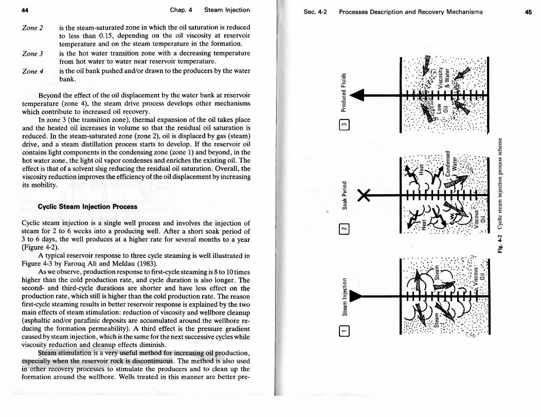
44
Zone2
Zone3
Zone 4
Chap.4 Steam Injection
is the steam-saturated zone in which the oil saturation is reduced to less than 0.15, depending on the oil viscosity at reservoir temperature and on the steam temperature in the formation. is the hot water transition zone with a decreasing temperature from hot water to water near reservoir temperature . is the oil bank pushed and/or drawn to the producers by the water bank.
Beyond the effect of the oil displacement by the water bank at reservoir temperature (zone 4), the steam drive process develops other mechanisms which contribute to increased oil recovery.
In zone 3 (the transition zone), thermal expansion of the oil takes place and the heated oil increases in volume so that the residual oil saturation is reduced. In the steam-saturated zone (zone 2), oil is displaced by gas (steam) drive, and a steam distillation process starts to develop. If the reservoir oil contains light components in the condensing zone (zone 1) and beyond, in the hot water zone, the light oil vapor condenses and enriches the existing oil. The effect is that of a solvent slug reducing the residual oil saturation. Overall, the viscosity reduction improves the efficiency of the oil displacement by increasing its mobility.
Cyclic Steam Injection Process
Cyclic steam injection is a single well process and involves the injection of steam for 2 to 6 weeks into a producing well. After a short soak period of 3 to 6 days, the well produces at a higher rate for several months to a year (Figure 4-2).
A typical reservoir response to three cycle steaming is well illustrated in Figure 4-3 by Farouq Ali and Meldau (1983).
As we observe, production response to first-cycle steaming is 8 to 10 times higher than the cold production rate, and cycle duration is also longer. The second- and third-cycle durations are shorter and have less effect on the production rate, which still is higher than the cold production rate. The reason first-cycle steaming results in better reservoir response is explained by the two main effects of steam stimulation: reduction of viscosity and wellbore cleanup (asphaltic and/or parafinic deposits are accumulated around the wellbore reducing the formation permeability). A third effect is the pressure gradient caused by steam injection, which is the same for the next successive cycles while viscosity reduction and cleanup effects diminish.
Steam stimulation is a very useful method for increasing oil production, especially when the reservoir rock is discontinuous. The method is also used in other recovery processes to stimulate the producers and to clean up the formation around the wellbore. Wells treated in this manner are better pre-
Sec. 4-2
•
Processes Description and Recovery Mechanisms
~ 0
·;:: C1)
c.. -""' ca 0
en
E1
c: .g u C1)
"2
E ca C1) .... en
:~r.,~~~ ·~ A/·\~· -: . . .
., a ., .c (.)
"' ~ ., (.)
8 P. c .2 ti ., :sa ca 2 "' -~ c
45

46
Cl 60 ~
"' -- a: cc
"' ..,; .... 40 e. "' a: a..
Cl
20
E "' ~
en Cycle - 1
8 16
Chap.4
24 Months
Steam Injection
32
Fig. 4-3 Typical cyclic steaming performance (From Farouq Ali and Meldau, 1983)
pared for picking up the fluid bank displaced by a burning front in a process of in situ combustion, for instance. When the productive formation is continuous, some operators convert steam stimulation to steam drive, after a couple of cycles, to increase the oil recovery. Sometimes, when shallow oil reservoirs have a thick productive formation or high dip and good lateral permeability, the cyclic steam injection operation results in a higher oil recovery. In these cases the steam cycles repeated at the beginning, in closely spaced wells, transmit the heat through the oil beyond the normal drainage area of the well (Figure 4-4). The new drainage areas of two neighboring steam-stimulated producers overlap.
Interwell communication determines the oil to flow under the influence of the gravitational effect (Seba and Perry, 1969). This very efficient mechanism results in high re~overies.
Producer Producer
Fig. 4-4 Cyclic steam stimulated producers with drainage area overlapped and gravitational effect in place
Sec. 4-3 Heat Amount to the Formation 47
4-3 HEAT AMOUNT TO THE FORMATION
As pointed out in Chapter 3, the heat losses in a steam injection system begin at the steam generator and continue to the surface injection lines , to the wellbore, and to the adjacent strata. The remaining heat is given up to the formation itself, and some of it is transported with the fluids produced.
The beneficial effect of steam injection on oil displacement and recovery depends on the amount of heat transferred to the formation itself and on the porous volume swept by the hot fluids. To evaluate this effect the amount of heat loss to adjacent strata must be known. The first results of mathematical heat models of heat transfer and heat loss in the formation were published by Lawerier (1955), Marx and Langenheim (1959), Rubinstein (1959), and Willman et al. (1961). Gates and Ramey (1964) and Ramey (1965) have made a graphical comparison of these results by plotting on a Cartesian scale the fraction of total heat injected lost to adjacent strata, w: versus the logarithm of the dimensionless time function, t0 (Figure 4-5). The dimensionless time is defined as
4D X t to= h2 dimensionless
where
t = time, days D = thermal diffusivity of the cap rock, ft2/day h = formation thickness, ft
(4-1)
The amount of heat lost to adjacent strata varies directly with time of injection and inversely with formation thickness. So the heat lost can be a high percentage of the cumulative heat injected in a steam drive process's lifetime. To reduce the amount of heat lost to adjacent strata, a process of heat scavenging is accomplished by displacing the hot fluids "slug" with cold water injection. The process is also useful for saving energy when the formation is heated and the steam breaks through into the producers.
Gates and Ramey (1964) expressed the cumulative heat loss resulting from injection of hot fluid from time zero to time t0 , followed by injection of cold fluid from time t0 to time t as:
(Wo)t = t[<w:)t- (t ~to )<wn~-~.J (4-2)
where
(Wo)t = fraction of total heat injected in "slug" up to time t that is lost t = total time of injection (hot and cold fluid) , days
to = time heat was injected, days w : = is obtained from Figure 4-5 at times t and t - t0 •
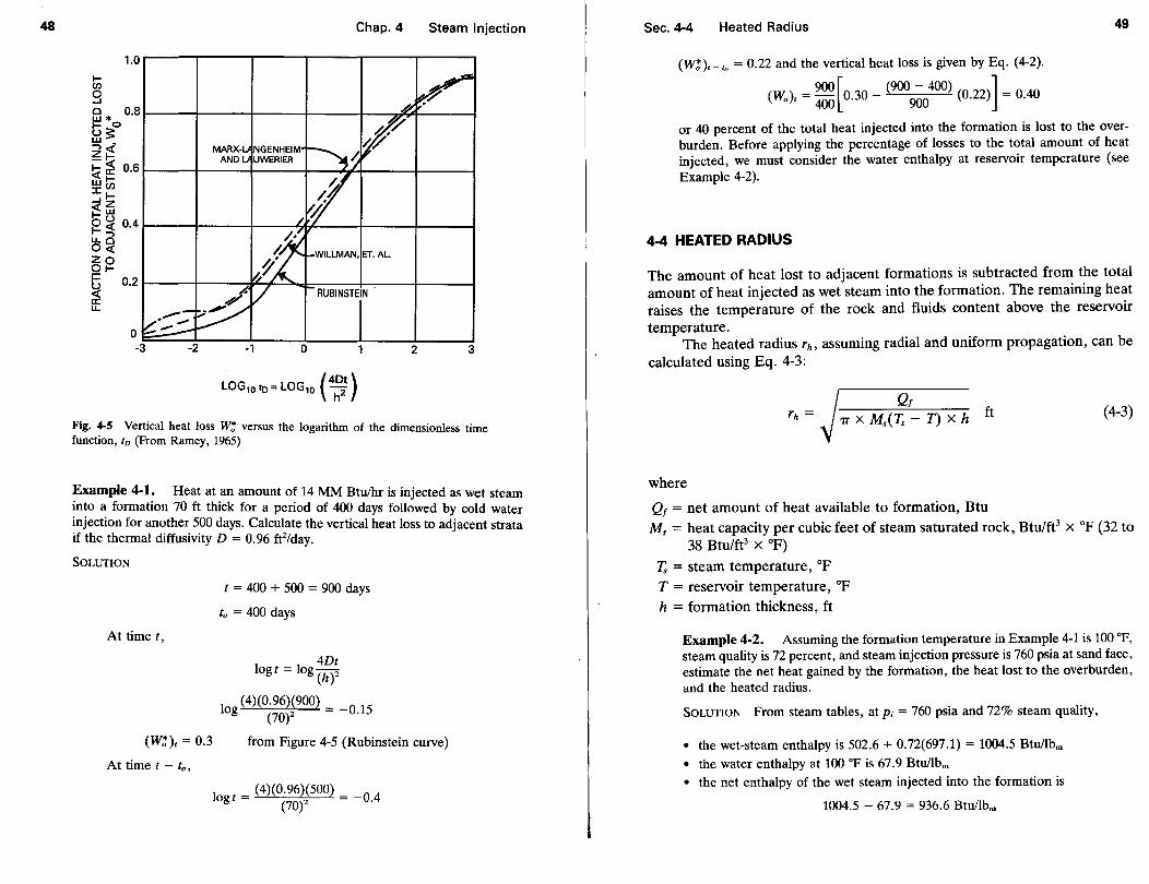
48 Chap.4 Steam Injection
1.0 .....----.----.-----.---..-----....------.
(4Dt) LOG10 to= LOG 10 h2
Fig. 4-5 Vertical heat loss w: versus the logarithm of the dimensionless time function, tv (From Ramey, 1965)
Example 4-1. Heat at an amount of 14 MM Btu/hr is injected as wet steam into a formation 70 ft thick for a period of 400 days followed by cold water injection for another 500 days. Calculate the vertical heat loss to adjacent strata if the thermal diffusivity D = 0.96 ft2/day.
SOLUTION
At timet,
t = 400 + 500 = 900 days
to= 400 days
4Dt logt =log (h)2
I (4)(0.96)(900) = -O 15 og (70)2 .
(W: ), = 0.3 from Figure 4-5 (Rubinstein curve)
At timet - to,
I - (4)(0.96)(500) - 0 4 og t - (70)2 - - .
Sec. 4-4 Heated Radius 49
(W:). _ 'o = 0.22 and the vertical heat loss is given by Eq. (4-2).
900 [ (900 - 400) ] -(Wo)t = 400 0.30 - 900 (0.22) - 0.40
or 40 percent of the total heat injected into the formation is lost to the overburden. Before applying the percentage of losses to the total amount of heat injected, we must consider the water enthalpy at reservoir temperature (see Example 4-2).
4-4 HEATED RADIUS
The amount of heat lost to adjacent formations is subtracted from the total amount of heat injected as wet steam into the formation. The remaining heat raises the temperature of the rock and fluids content above the reservoir temperature.
The heated radius rh, assuming radial and uniform propagation, can be calculated using Eq. 4-3:
1T X M.(T; - T) X h ft (4-3)
where
Q1 = net amount of heat available to formation, Btu M. = heat capacity per cubic feet of steam saturated rock, Btulft3 x oF (32 to
38 Btu/ft3 x °F)
I; = steam temperature' °F T = reservoir temperature, oF h = formation thickness, ft
Example 4-2. Assuming the formation temperature in Example 4-1 is 100 °F, steam quality is 72 percent, and steam injection pressure is 760 psia at sand face, estimate the net heat gained by the formation, the heat lost to the overburden, and the heated radius.
SOLUTION From steam tables, at p; = 760 psia and 72% steam quality,
• the wet-steam enthalpy is 502.6 + 0.72(697.1) = 1004.5 Btu/Ibm • the water enthalpy at 100 oF is 67.9 Btullbm • the net enthalpy of the wet steam injected into the formation is
1004.5 - 67.9 = 936.6 Btu/Ibm
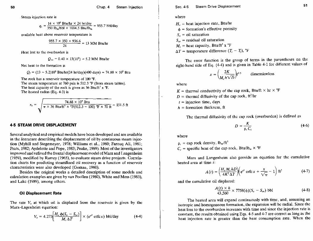
50 Chap.4 Steam Injection
Steam injection rate is
14 x 106 Btu/hr x 24 hr/day qs = 350 lbmlbbl X 1004.5 Btu/Ibm = 955 ·7 bbl/day
available heat above reservoir temperature is
955.7 X 350 X 936.6 _ 13
MM h 24
- Btu/ r
Heat lost to the overburden is
Qov = 0.40 X 13(106) = 5.2 MM Btu/hr
Net heat to the formation is
Q1 = (13 - 5.2)106 Btu/hr(24 hr/day)(400 days) = 74.88 x 10⁹ Btu
The rock has a reservoir temperature of 100 °F. The steam temperature at 760 psia is 512.3 op (from steam tables). The heat capacity of the rock is given as 36 Btulfe x oF.. The heated radius (Eq. 4-3) is
74.88 X 10⁹ Btu 1T X 36 Btulfe X °F(512.3 - 100) op X 70 ft = 151.5 ft
4-5 STEAM DRIVE DISPLACEMENT
Several analytical and empirical models have been developed and are available in the literature describing the displacement of oil by continuous steam injection (Myhill and Stegemeyer, 1978; Williams et al., 1980; Farouq Ali, 1981; Prats, 1982; Aydelotte and Pope, 1983; Peake, 1989). Most of the investigators improved and refined the frontal displacement model of Marx and Langenheim (1959), modified by Ramey (1965), to evaluate steam drive projects. Correlation charts for predicting steamflood oil recovery as a function of reservoir characteristics were also developed (Gomaa, 1980).
Besides the original works a detailed description of some models and calculation examples are given by van Poollen (1980), White and Moss (1983), and Lake (1989), among others.
Oil Displacement Rate
The rate Va at which oil is displaced from the reservoir is given by the Marx-Lagenheim equation:
V, = 4.273[Ha<l>z.oA; Sa,)] X (e2 erfcx) bbl/day (4-4)
Sec. 4-5 Steam Drive Displacement
where
Ho = heat injection rate, Btu/hr <1> = formation's effective porosity
So = oil saturation S0 , = residual oil saturation Ms = heat capacity' Btu/ft3
X op
AT= temperature difference (7; - Tr), op
51
The error function is the group of terms in the parentheses on the right-hand side of Eq. (4-4) and is given in Table 4-1 for different values of
x = ( ZK )t0·5 dimensionless MshVf5
where
K = thermal conductivity of the cap rock, Btu/ft x hr X op
D = thermal diffusivity of the cap rock, felhr
t = injection time, days h = formation thickness, ft
The thermal diffusivity of the cap rock (overburden) is defined as
where
Pc = cap rock density, lbm/ft3
Cc = specific heat of the cap rock, Btu/Ibm X op
(4-6)
Marx and Langenheim also provide an equation for the cumulative heated area at time t:
A(t) = (~:~~)(e2 erfcx + ~- 1) ft2 (4-7)
and the cumulative oil displaced:
A(t) X h 43
,560
X 7758(<J>)(S0 - S0 ,) bbl (4-8)
The heated area will expand continuously with time, and, assuming an isotropic and homogeneous formation, the expansion will be radial. Since the heat loss to the overburden increases with time and since the injection rate is constant, the results obtained using Eqs. 4-5 and 4-7 are correct as long as the heat injection rate is greater than the heat consumption rate. When the

Ul N
TABLE 4-1. Error Function Values
e-"2 erfcx 2 2t X ex erfcx + y:;;: - 1
0.00 1.00000 0.00000 .02 .97783 .00039 .04 .95642 .00155 .06 .93574 .00344 .08 .91576 .00603
0.10 0.89646 0.00929 .12 .87779 0.1320 .14 .85974 .01771 .16 .84228 .02282 .18 .82538 .02849
0.20 0.80902 0.03470 .22 .79318 .04142 .24 .77784 .04865 .26 .76297 .05635 .28 .74857 .06451
0.30 0.73460 0.07311 .32 .72106 .08214 .34 .70792 .09157 .36 .69517 .10139 .38 .68280 .11158
0.40 0.67079 0.12214 .42 .65912 .13304 .44 .64779 .14428
.46 .63679 .15584
.48 .62609 .16771 0.50 0.61569 0.17988
.52 .60588 .19234
.54 .59574 .20507
.56 .58618 .21807
.58 .57687 .23133 0.60 0.56780 0.24483
.62 .55898 .25858
.64 .55039 .27256
.66 .54203 .28676
.68 .53387 .30117 0.70 0.52593 0.31580
.72 .51819 .33062
.74 .51064 .34564
.76 .50328 .36085
.78 .49610 .37624 0.80 0.48910 0.39180
.82 .48227 .40754
.84 .47560 .42344
.86 .46909 .43950
.88 .46274 .45571 0.90 0.45653 0.47207
.92 .45047 .48858
.94 .44455 .50523
.96 .43876 .52201
.98 .43311 .53892
From Marx and Langenheim (1959).
X
1.00 .05 .10 .15 .20
1.25 .30 .35 .40 .45
1.50 .55 .60 .65 .70
1.75 .80 .85 .90 .95
2.00 .05 .10
.15
.20 2.25
.30
.35
.40
.45 2.50
.60
.70
.80
.90 3.00
.10
.20
.30
.40 3.50
.60
.70
.80
.90 4.00
.10
.20
.30
.40
e-"2 erfcx x2 rf 2t 1 ex2 erfcx 2 2t e e ex+-- X ex erfc X + y:;;: - 1 y:;;:
0.42758 0.55596 4.50 0.12248 4.20019 .41430 .59910 .60 .11994 .31048 .40173 .64295 .70 .11749 .42087 .38983 .68746 .80 .11514 .53136 .37854 .73259 .90 .11288 .64194
0.36782 0.77830 5.00 0.11070 4.75260 .35764 .82454 .20 .10659 4.97417 .34796 .87127 .40 .10277 5.19602 .33874 .91847 .60 .09921 .41814 .32996 .096611 .80 .09589 .64049
0.32159 1.01415 6.00 0.09278 5.86305 .31359 .06258 .20 .08986 6.08581 .30595 .11136 .40 .08712 .30874 .29865 .16048 .60 .08453 .53184 .29166 .20991 .80 .08210 .75508
0.28497 1.25964 7.00 0.07980 6.97845 .27856 .30964 .20 .07762 7.20195 .27241 .35991 .40 .07556 .42557 .26651 .41043 .60 .07361 .64929 .26084 .46118 .80 .07175 7.87311
0.25540 1.51215 8.00 0.06999 8.09702 .25016 .56334 .20 .06830 .32101 .24512 .61472 .40 .06670 .54508
.24027 .66628 .60 .06517 .76923
.23559 .71803 .80 .06371 8.99344 0.23109 1.76994 9.00 0.06231 9.21772
.22674 .82201 .20 .06097 .44206
.22255 .87424 .40 .05969 .66645
.21850 .92661 .60 .05846 9.89090
.21459 1.97912 .80 .05727 10.11539 0.21081 2.03175 10.00 0.05614 10.33993
.20361 .13740 ·.19687 .24350 .19055 .35001 .18460 .45690
0.17900 2.56414 .17372 .67169 .16873 .77954 .16401 .88766 .15954 2.99602
0.15529 3.10462 .15127 .21343 .14743 .32244 .14379 .43163 .14031 .54099
0.13700 3.65052 .13383 .76019 .13081 .87000 .12791 3.97994 .12514 4.09001

54 Chap.4 Steam Injection
so-called critical time period is reached, steam drive projects are evaluated using more complex models.
Example 4-3. An isotropic and homogeneous oil reservoir is subjected to a steamdrive process in which 1200 bbl!day wet steam of 80 percent quality is injected at 660 psia into 65ft of productive formation. Calculate the oil displaced by steam drive and the cumulative heated area if the injection period is 5 years and the reservoir rock characteristics are as follows:
Porosity <l> = 26% Oil saturation at start of the process Sa = 0.60 Residual oil saturation in steam zone Reservoir temperature Heat capacity Thermal diffusivity
Sor = 0.12 T = 130 OF
M, = 32 BtuJfe x OF D = 0. 70 ft2/day
Thermal conductivity K = 0.95 Btu!ft x hr x oF
SOLUTION The argument of the error function, x, is
X = ( 2 X 0.95 ) to.s = O.QQ53to.s 32 X 65v'O. 70/24
Heat injection rate, Ha is
where
q, = steam injection rate, bbl/day [s = steam quality, decimal fraction
htg = enthalpy of vaporization (tables) h1 = enthalpy of saturated liquid (tables)
hr••r = enthalpy of water at initial reservoir temperature (tables)
C = 350 lbmlbbl = 14.583 Ibm X day 24 hr/day bbl x hr
(4-9)
Ho = 14 583 (Ibm) day x 1200 bbl!day x 960.54 Btu/Ibm = 16.808 MM Btu/hr · bbl (hr)
Rate of oil displaced, Va (bbl/day) is
V =
4 275 hr bbl(10 x 106)(0.26)(0.60- 0.12) Btu!hr(ex2 erfcx)
o • day ft3 35 Btu/ft3 x oF ( 496.58 - 130) oF
Vo = 698.5(ex2 erfcx)
where
X = (Q.QQ53)Vt
and t is introduced in hours.
I ~ :j 1:
Sec. 4-5 Steam Drive Displacement 55
TABLE 4-2. Oil Displaced by Steam Drive
Oil Displaced
Time Barrels Barrels Cumulative Oil Steps (days) X ex2 erfcx * per Day per Step per Barrel
1 1 0.0259 0.9715 678.6 678.6 679 2 50 0.1836 0.8224 574.4 30,698 31,377 3 100 0.2596 0.7632 533.1 27,687 59,064 4 200 0.3672 0.6907 482.4 50,775 109,839 6 600 0.6360 0.5521 385.6 173.600 283,439 8 1000 0.8211 0.4819 336.6 144,440 427,879
10 1400 0.9715 0.4338 303.0 127,920 555,799 12 1825 1.1092 0.3995 279.0 123,675 679,474
*By interpolating the error function values (Table 4-1).
The oil displaced by steam drive is given in Table 4-2 at different time increments.
The cumulative heated area after 5 years of steam injection is given by Eq. 4-7.
A()= 16.808 x 10⁶ Btu/hr(32Btu/ft3 x °F)65ft(0.70/24)ft%r t 4(0.95Btu/ft X hr X °F)2(496.58- 130)°F
( e 2 erfc X + ~ - 1)
= 770,531 ft2(0.65114) = 501,723 ft2
The cumulative oil displaced (Eq. 4-8) is
501,723 ft2 X 65ft 43
,560
ft3/acre x 7758 bbl/acre(0.26)(0.60 - 0.12) = 724,860 bbl
The cumulative oil displaced corresponds to the entire thickness of the formation. In reality, as we saw, less oil is displaced since the steam segregates
· gravitationally and overrides. However, oil displaced does not mean oil produced. Areas of reservoir rock between producers or the lower half of the formation thickness can receive some of the displaced oiL In a real oil reservoir, nonuniformity of displacement and bypass regions of high oil saturation do occur.
Oil Recovery, Oil-Steam Ratio
Correlation charts for predicting steamflood oil recovery and oil-steam ratio have been developed by Gomaa (1980) using reservoir simulation.
The first step in estimating the oil recovery using Gomaa's charts

.... ::::l c. c:: -0
a'< ... ... 0
...J .... "' "' ::c ;;; u .E "' >
56 Chap.4 Steam Injection
100
80 ~
~ ~ 60
40
" ~ ~ \\ ~ ~ Heat Injection Rate \ ~~ ~ ~.05- ,/" MMBtu./D/Acre Ft.
'\ ~ ~-1 ~ ~ .2
20 " "- ~ ~ t::::: ~ ~-4 "'"' .6
~ ~ ~""'--I'--
fi r--0 0 40 80 120 160 200 240 280 320
Reservoir Thickness, Feet
Fig. 4-6 Heat loss to overlying and underlying strata (From Gomaa, 1980)
and equations is to read the vertical heat loss (fhv) to adjacent strata from Figure 4-6.
For instance, for a gross reservoir thickness of 100ft and heat injection rate of 0.05 MM Btu/day x acre X ft, the heat loss to vertical adjacent strata is 40 percent of input.
The next step is to read the heat utilization factor Y from Figure 4-7. The heat utilization factor is a function of steam quality and is defined
by Gomaa as the ratio of the effective heat injected to the net heat injected for each steam quality value:
(4-10)
The effective heat injected (Q.) is the fraction of the net heat injected (Qini) utilized effectively in the reservoir.
The net heat injected for each time increment t:J.t is given by
Qini = 0.128q,h(1 - fhv)!:i.t MM Btu/day acre-ft
where
q, = injection rate, bbl/day acre-ft h =wet-steam enthalpy, Btu/lbm (tables)
fhv = vertical heat loss, fraction !:J.t = time increments, years
(4-11)
Sec. 4-5 Steam Drive Displacement
>=" 1.0 ..... 0 .... ..., "' L.L
c::
-~ 0. "' N
·.;:::; ::;) .... "' "' ::c o.
8v 6
0
~
v r--....... r----...... ~
0.2 0.4 0.6 Injected Steam Quality
57
.......... ~
..........
0.8 1.0
Fig. 4-7 Heat utilization factor as a function of steam quality (From Gomaa, 1980)
Now, the effective heat injected can be calculated and used to read the oil recovery factor from Figure 4-8, as a function of different initial values of mobile oil saturation defined by Gomaa (1980) as
where
S0 ; = initial oil saturation prior to steam drive operation S0 , = residual oil saturation in the steam zone.
( 4-12)
Example 4.4. Estimate the oil recovery factor after 4 years of wet-steam injection of 0.8 quality with a constant rate of 4900 bbl/day at 820 psia sand-face injection pressure. Other data are as follows:
Reservoir productive area 100 acres
Reservoir thickness Gross Effective
Oil saturation at start of process Residual oil saturation in steam zone Reservoir temperature (initial)
SOLUTION
43ft 25ft 0.58 0.08 95 °F
The wet-steam enthalpy is given by Eq. 3-5 and by subtracting the water enthalpy at initial reservoir temperature: h = 513.2 Btu/Ibm + 0.8(684.8) Btu/Ibm - 62.98 Btu/Ibm = 998.06 Btu/Ibm, and the heat injected per day per acre-ft is
998.06 Btu 4900 bbl/day x 350 lbmlbbl X 10.0 acres X 43 ft X Ibm
= 398,063 or 0.39806 MM Btu/day x acre x ft
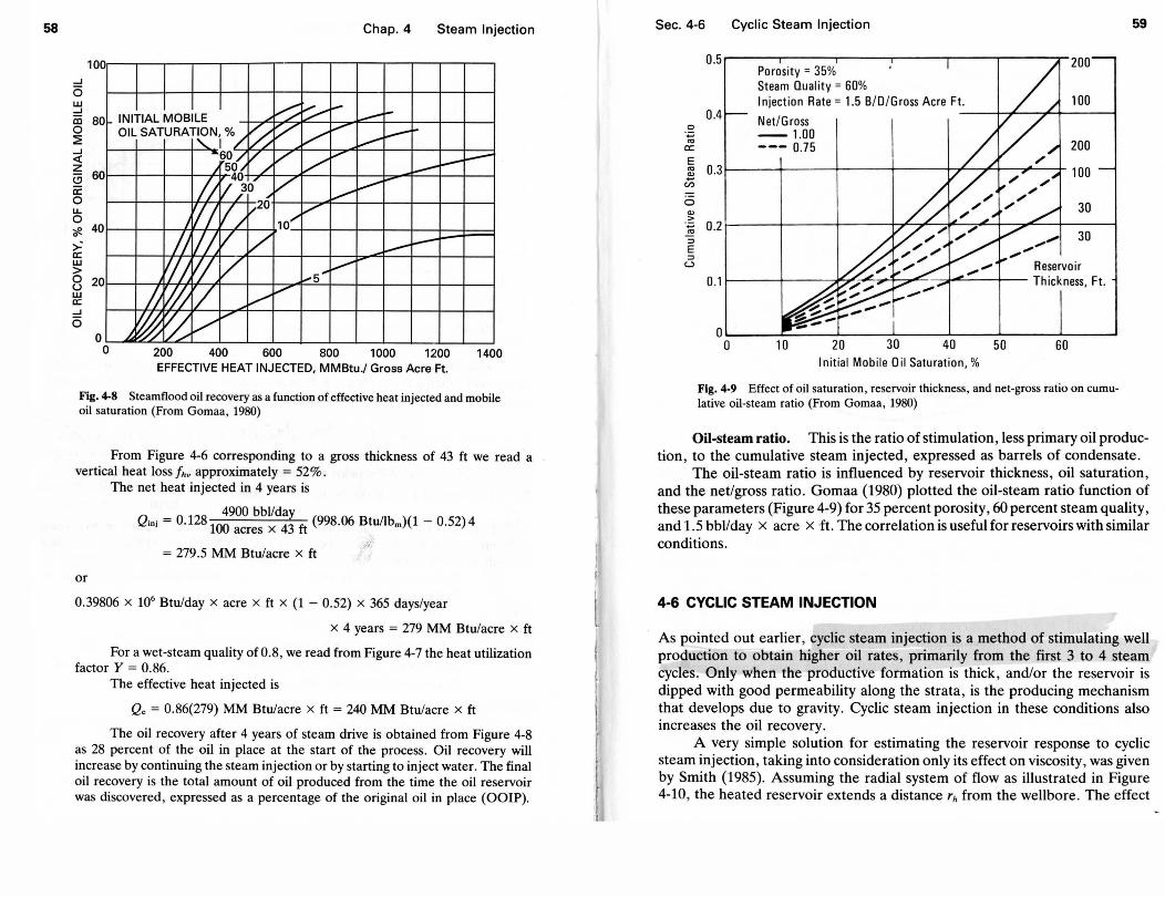
58
...J
0 w ...J co 0 ::2 ...J
< z a a: 0 u. 0 <ft. > a: w > 0 u w a: ...J
0
100
80
60
40
20
0 0
Chap.4 Steam Injection
0-~ - ---INITIAL MOBILE OIL SATURAT~N~% / ~ / v ........ --~-v
-6o/v / v ...... 1--50j / ~ !J 40 v v 'lV}o~ v
,'/IV /v2o 10 ..... v
II II v v v ~ If~ lj v :,s .... v
/; '!/; '/ y v
@ ~ v I-'
~ 200 400 600 800 1 000 1200 EFFECTIVE HEAT INJECTED, MMBtu./ Gross Acre Ft.
~
1400
Fig. 4-8 Steamflood oil recovery as a function of effective heat injected and mobile oil saturation (From Gomaa, 1980)
From Figure 4-6 corresponding to a gross thickness of 43 ft we read a vertical heat loss [h. approximately = 52%.
The net heat injected in 4 years is
_ 4900 bbl/day Qini - 0.128 100 acres X 43 ft (998.06 Btu/lbm)(1 - 0.52) 4
= 279.5 MM Btu/acre x ft
or
0.39806 x 10⁶ Btu/day x acre x ft x (1 - 0.52) x 365 days/year
x 4 years = 279 MM Btu/acre X ft
For a wet-steam quality of0.8, we read from Figure 4-7 the heat utilization factor Y = 0.86.
The effective heat injected is
Q. = 0.86(279) MM Btu/acre x ft = 240 MM Btu/acre x ft
The oil recovery after 4 years of steam drive is obtained from Figure 4-8 as 28 percent of the oil in place at the start of the process. Oil recovery will increase by continuing the steam injection or by starting to inject water. The final oil recovery is the total amount of oil produced from the time the oil reservoir was discovered, expressed as a percentage of the original oil in place (OOIP).
Sec. 4-6 Cyclic Steam Injection
0.5r-----r-----r----r----r---r------.,-200 Porosity = 35% Steam Quality= 60% Injection Rate = 1.5 B/0/G ross Acre Ft. 100
0.4 Net/Gross ---+-~-T-+-----1 -~ --1 .00 r!i. --- 0.75 200 E ~ 0.31---+-----l---+----++---::,.c..+---;--+ 100
ci5 0
"' 30
·~ 0 .21---+-----lf-----h~_,L-~~~Y--7"!::......-+-----l .!2. ::::l E ::::l
u
30
Reservoir 0.1 r-----+---~1'7"...,..~"1-::7""-"'- -..,..;...c_--+-- Thickness, Ft.
60
Initial Mobile Oil Saturation, %
Fig. 4-9 Effect of oil saturation , reservoir thickness, and net-gross ratio on cumulative oil-steam ratio (From Gomaa, 1980)
59
Oil-steam ratio. This is the ratio of stimulation, less primary oil production, to the cumulative steam injected, expressed as barrels of condensate.
The oil-steam ratio is influenced by reservoir thickness , oil saturation, and the net/gross ratio. Gomaa (1980) plotted the oil-steam ratio function of these parameters (Figure 4-9) for 35 percent porosity, 60 percent steam quality, and 1.5 bbl/day x acre x -ft. The correlation is usefulfor reservoirs with similar conditions.
4-6 CYCLIC STEAM INJECTION
As pointed out earlier, cyclic steam injection is a method of stimulating well production to obtain higher oil rates , primarily from the first 3 to 4 steam cycles. Only when the productive formation is thick, and/or the reservoir is dipped with good permeability along the strata, is the producing mechanism that develops due to gravity. Cyclic steam injection in these conditions also increases the oil recovery.
A very simple solution for estimating the reservoir response to cyclic steam injection, taking into consideration only its effect on viscosity, was given by Smith (1985). Assuming the radial system of flow as illustrated in Figure 4-10, the heated reservoir extends a distance rh from the wellbore. The effect

60
Po cold
unheated area
Chap.4 Steam Injection
Fig. 4-10 Idealized sketch of heated area around a cycling steam injection well
of the heated zo?e on well productivity can be understood by picturing a system ~~two concentnc hollow cylinders of radii r and r,, with a pressure drop given
where
Pe- Pw = {p,- p) + {p - Pw) (4-13)
Pe - Pw = pressure drop before the first steam injection cycle (reservoir cold)
(p e - P) + (p - Pw) = pressure drop after the steam cycle injection
~sing Darcy'~ law to express the oil rate before (q0 cotd), and after (q0
ho•),
the ratio q 0 hot/q0 cold IS
q 0 hot = IJ-0 cold ln(r)rw) q0 coid IJ-0 hot ln(rhlrw) + IJ-0 coid ln(r/rh) (4-14)
where IJ.o is the oil viscosity value in both heated and unheated areas. The heated radius rh can be calculated using Eq. 4-3.
Sec. 4-7 Field Development and Results 61
Example 4-5. Calculate the productivity increase of a well which produces oil from Kern River reservoir with 1100 cp initial viscosity, assuming after the first cycle of steam injection that
Heated radius 47 ft Reservoir temperature Reservoir temperature of heated area Drainage radius Wellbore radius
100 °F
300 °F 700ft 3.5/12 ft
SOLUTION The temperature-viscosity relationship for the Kern River oil reservoir (Fig. 3-10) shows that oil viscosity in the heated zone decreases to 10 cp. The increase in the well's productivity is
q0 hot = 1100 cp ln(700/0.29) _ . q
0cotd 10 ln(47/0.29) + 1100 ln(700/47) - 2'83 ttmes
and is due only to the decrease of the oil viscosity. The productivity of the well is also improved by the steam's wellbore cleanup effect, which increases the rock permeability around the wellbore.
4-7 FIELD DEVELOPMENT AND RESULTS
The field development of steam injection, as cyclic steam injection and as steam drive, has made an impact on 1988 EOR oil production in the United States. About 80 percent of total EOR production-or 455,484 bbllday additional oil-can be attributed to 133 active processes using these methods (Lake, 1989).
The development of steam injection field projects covers oil reservoirs with a variety of characteristics in different exploitation phases. The evolution and current status of steamflooding has been presented by many investigators: Farouq Ali and Meldau (1979), Matthews (1983), and Chu (1985), among others. The method has been applied to reservoirs having
• depth between 200ft (Charco Redondo, Texas) and 5000 ft (Brea, California)
• formations of sand and sandstones • average gross thickness between 30 ft (Slocum, Texas) and 550 ft (Brea,
California) • dip between 0° (Huntington Beach and Inglewood, California) and 70°
(Midway Sunset, California-Tenneco) • porosity between 20 percent (Shiells, California) and 38 percent (Tiajuana,
Mexico)

62 Chap.4 Steam Injection
• absolute permeability between 70 md (Brea, California) and 15,000-24,000 md (Mount Poso, California)
Most steam injection operations have been applied to heavy crude oil reservoirs with densities between 12 and 18 o API and viscosities between 600 to 6000 cp in reservoir conditions. The main objectives were to increase oil production by reducing oil viscosity and to increase oil recovery by steam displacement. Steam injection has also been applied to reservoirs with light and intermediate crude oils with 20 to 40 o API densities and low viscosities, that is, Brea, California, with 24 °API and 6 cp. ElDorado, Kansas, with 37 °API and 4 cp; and Shiells Canyon, California, with 34 °API density and 6-cp viscosity (Chu, 1985). Steam injection in these applications is known as steam distillation drive. Its primary objective is to reduce the residual oil saturation below that obtainable by waterflooding and to increase the oil recovery. Other field tests and processes of steam injection, especially cyclic steam injection, have been developed, particularly in Canada, to recover bitumen from tar sands.
Characteristics and results of steam injection are presented through four examples of field applications:
• The Kern River steam foam pilots project, in which foam is utilized to retard steam override
• The "200" Sand steamflood project, which is a typical heavy oil reservoir which had unfavorable response to cyclic stimulation
• The Pikes Peak very viscous oil reservoir, which is an example of conversion from cyclic steam to steam drive. . ..
• The steam injection for recovery of bitumen fr~~ttar sands.
Kern River Steam Foam Pilots, California, United States
Two large-scale steam foam pilots (one on the Mecca Lease and the other on the Bishop Fee) were conducted in the Kern River Field, and the evaluated data and results were presented by Patzek and Koinis (1988).
The Reservoir. The Kern River oil field located near Bakersfield, California, has three productive sand intervals, named "J," "M," and "Q" sands. Figure 4-11 presents the type log of "M" and "Q" sands where the Mecca and Bishop pilots took place, respectively. The two pilots each consisted of four inverted five-spot patterns with a total area of 11.6 acres at Mecca and 14 acres at Bishop. The formation is 3° SW dip and has 30 percent porosity, 70 percent
Sec. 4-7 Field Development and Results 63
Induction Induction
l' •.
1--..,......--"J"
Fig. 4-11 Mecca and Bishop type logs (From Patzek and Koinis, 1988)
initial oil saturation, and 13 o API gravity oil. The formation's gross thickness differs, being 83ft at Mecca and 99ft at Bishop, and is situated at 1000 ft depth and at 600 ft depth, respectively.
Performance. The production and injection history of the Mecca pilot prior to foam injection is represented by a recovery of 6.8 percent of OOIP in primary, with 15.0 percent of OOIP additional oil as a result of? !ears ~f cyclic steam injection, and with another 28.7 percent of OOIP additional ml as result of a 10-year steam drive period.
The Bishop pilot area has a recovery of 8 percent of OOIP in primary, with 55.2 percent of OOIP additional oil as a result of 19 years' cyclic steam injection and with 1. 9 percent of 00 IP additional oil after only 1 year of steam
drive.
Steam foam pilots. The purpose of steam foam pilots was to retar? steam override, increase vertical sweep, and increase oil production and od recovery consequently.
Foams are dispersions of gas bubbles, air, or only nitrogen in water (steam) with surfactant. Foam forms downhole after the injection of ~hemicals. The presence of foam in the reservoir's pore space reduces the relative permeability to steam, and steam foam fluid has a lower mobility than steam.
? ~;'

Cl
---cc ~ "' a: ·-0
64 Chap.4 Steam Injection
500
450
400
350
300
250
200
150
100
50 Start Chemicals
~ ......................................................
0 7 8 9 10 11 12 13 14 15 16
Years from Start of Steam Drive
Fig. 4-12 Mecca steam foam pilot (From Patzek and Koinis, 1988)
Results. The increase in oil production is illustrated in Figure 4-12 for the Mecca pilot and represents 14 percent of OOIP additional oil after 5 years of steam foam injection.
The increase in oil production for the Bishop pilot was 8.5% of OOIP additional oil after 3.7 years of steam foam injection with infill drilling and cyclic steam stimulation.
The increase in vertical sweep is illustrated by Patzek and Koinis in Figures 4-13 and 4-14 using simultaneous temperature surveys and gammaray-neutron logs run in the observation wells.
The steam foam presence in the porous space means an increase in gas saturation detected by the neutron log. As we can observe, steam override was .retarded and vertical sweep increased.
The residual oil saturation when using steam foam was 10 percent in both pilots. This value is practically the same as that when using steam. Steam foam injection's effect of increasing the oil recovery is consequently due to the increase of sweep efficiency and not to the reduction of residual oil saturation.
Comments. The experience gained using steam foam injection in the field is very useful and shows that
• Steam foam injection retards steam override and increases vertical sweep, even after a long period of steam drive.
Sec. 4-7 Field Development and Results
.... LL.
-;:; a. "' Cl
"" 0 _.
600
15 Months of Foam
Bishop Observation Well T5
24 Months of Foam
30 Months of Foam
650
150 225 300 150 225 300 150 225 Tem"perature (F)
Fig. 4-13 Improved vertical sweep by steam foam 70ft from injector (From Patzek and Koinis, 1988)
65
300
• Oil production is increased and oil recovery is enhanced by better vertical sweep efficiency.
• Infill drilling is necessary to improve the injection-production balance if the economic conditions for drilling new wells are acceptable.
• Cyclic steam injection is still used to clean old wellbore wells or to link new cold producers with the effect of injectors.
The "200" Sand, Midway Sunset Steamflood, California, United States
Steam injection has been applied with good results in Midway Sunset Field reservoirs. However, there were still shallow heavy oil reservoirs in this field with poor cyclic steam performance and, for this reason, not adequately developed.
The so-called "demonstration project" was initiated in the "200" Sand reservoir "to demonstrate the operational, recovery, and economic aspects of steamflooding" (Gagner, 1986).

66
N 1-1-
"' $: <= 0
·.;:::;
"' i:: ~
..c 0
"' u u "' :2 .... "' .~ a: E "' :..:::
.,E/_
.... "' "' 0
>~ ~ 0
~
"' E "' "' >-o LL.
'-'"! ..... ~ 0
"' ..r:::. E .... "' <=
0 0 :2LL. c.c
..... 0
"' .... "'
..... 0
"' "' >- -~ ~Cl .._ E Q) "' .... "' ~u;
0 0 0
0 on 0
0 0
Chap.4 Steam Injection
f~ t
~ "' 0 .... 0 ::::> N...,
E "' c.
o E on "' ~ 1-
Sec. 4-7 Field Development and Results 67
The reservoir. The "200" Sand Midway Sunset oil reservoir consists of interbedded sands, conglomerates, silts, and diatomites, discontinuous laterally. The reservoir has a depth of 400 to 700ft, a productive area of 250 acres, and a gross thickness of 200ft (150ft effective). The 12 °API oil gravity has 6500-cp viscosity at reservoir temperature (90 °F). The viscosity is reduced to 60 cp when the temperature is increased to 210 °F. The oil in place corresponding to a porosity of 30 percent, and average oil saturation of 59 percent is 51.4 million bbl.
Performance. The "200" sand has a very good permeability, with values between 1000 and 3400 md. However, even with the sharp decrease of oil viscosity with temperature increase and favorable flowing conditions, the primary oil production was far from satisfactory, and the reservoir response to cyclic steam stimulation was poor. A logical explanation was that the reservoir had a low average pressure value of 40 psig and consequently lacked enough energy to assure adequate production rates. Indeed, the "200" Sand Midway Sunset reservoir was the right choice to demonstrate steamflood performance.
The project. The pilot area started with 4 x 2.35-acre inverted seven~ spot steam drive patterns and was expanded in 1980-1981 to 14 fully developed patterns (Figure 4-15).
The project has been monitored and evaluated monthly through
+1400-
Fig. 4-15 Structural map at "200" sand steamflood project (Adapted from Gagner, 1986)

68 Chap.4 Steam Injection
10,000...---------------~ ..... ::-:--------, J-..._,./ '1
BSPD I ' Total Steam Injected I "\ rv-,
I ,J V\
'",.~"\,\{'J\,, I ~"'' 1000~--~~~~~--------~~~~--~------------~------~
Ill Ill Ill
Cumulative s/o Ratio
... ······· .............. : .. .
Yrs.
Fig. 4-16 Production and injection history "200" sand steamflood project (Adapted from Gagner, 1986)
production-injection data, through temperature and injection profiles run in observation wells, and through reports that have been prepared periodically. The project production and injection history reported by Gagner (1986) is illustrated in Figure 4-16.
Results. As we observe, the total oil production rate increased to an average of 150 bbllday (and 500 bbl/day water) after the first three years of continuous steam injection at a rate of 1000-1800 bbllday. Due to the heat energy accumulated in the formation, the recorded oil rate was over 100 bbl!day even when the injection rate was stoPJled for a period of time. When the steam rate was increased to 7000 bbllday, oil production reached 400 bbl!day (with 1700 bbllday water). Up to this point the reservoir responded to steam rate increases in only one way: The higher the injection rate, the higher the production. However, there was an injection rate value limit when steam breakthrough to producers occurred. Indeed a further increase of the injected steam rate to over 9000 bbl/day had a consequence of channelidg the injected steam to several producing wells and causing the decline of oil production to 280 bbl/day (with 270 bbllday water). To reduce steam channeling, the injection rate was reduced. At this time, as a direct result, the oil production rate went up to 460 bbllday (with 1920 bbllday water). The cumulative steam-oil ratio has decreased to 12 and is predicted to approach lower values as oil production increases.
Sec. 4-7 Field Development and Results 69
Comments. The experience gained from the "200" Sand steamflood project shows that
• The 14 injection wells completed with casing strings cemented to total depth are jet perforated at intervals restricted to 50 ft at the base of the formation for the first 4 wells and to 20ft for the next 10 wells. Limited-entry perforations in a heterogeneous formation with high-permeability stringers can cause severe channeling when the steam injection rates are high.
• The 42 producing wells (except 1) were completed with casing cemented at the top of the formation and with slotted liner and gravel packing along the entire formation. This configuration did not restrict production to the lower part of the formation to avoid steam override effect, since the formation is heterogeneous and there is no control of steam drive profile .
• The steam generated at 420 oF with 80 percent quality entered the formation at 350 °F sand-face temperature and 72 percent quality.
• The oil production was very sensitive to the back pressure on the formation. Wells had to be kept in pumped-off condition and cyclic steam injection had to be utilized to clean liner slots and the formations around the wellbore.
• The poor response of the downstructure producers was due to the poor formation characteristics in the corresponding injectors as revealed by high injection pressures. A more detailed geology and a well pattern adapted to the reservoir nonuniformity are important features to be considered in similar applications.
The "200" Sand Midway Sunset project demonstrated that shallow heavy oil reservoirs with poor cyclic steam performances could be developed by steamflooding.
Pikes Peak, High-Viscosity Oil Reservoir, Canada
The reservoir. Pikes Peak reservoir (Canada) is closer to being defined as a tar sand reservoir than an oil reservoir due to 25,000 cp viscosity of the oil (or bitumen) at 64°F reservoir temperature. The reservoir, located in Waseca formation of the Lloydminster area, has 1640-ft depth, an average net pay of 49ft with 32 to 36 percent porosity and 4500 to 10,000 md permeability. The reservoir description, the cyclic steam injection evaluation, and the conversion to steamflood are described by Miller and others (1989).
The project. The Pikes Peak oil reservoir consists of a homogeneous and highly permeable lower unit in communication with a sand/shale "A" interbeds unit. The reservoir was developed during a period from 1981 to 1987 by cyclic steam stimulation and 92 thermal wells drilled in a seven-spot pattern (Figure 4-17).
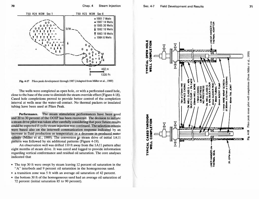
70
T50 R24 W3M Sec 1
Chap. 4 Steam Injection
T50 R23 W3M Sec 6
+ 1981 7 Wells .,.1987 14 Wells 0 1985 30 Wells A 1982 16 Wells
' 1983 19 Wells 1 1984 6 Wells
0 402 m
0 1320 Ft
Fig. 4-17 Pikes peak development through 1987 (Adapted from Miller et al. , 1989)
The wells were completed as open hole , or with a perforated cased hole , close to the base of the zone to diminish the steam override effect (Figure 4-18). Cased hole completions proved to provide better control of the completion interval at wells near the water-oil contact. No thermal packers or insulated tubing have been used at Pikes Peak.
Performance. The steam stimulation performances have been good and 20 to 30 percent of the OOIP has been recovered. The decision to initiate a steam drive pilot was taken after carefully considering that poor future results could be expected if cyclic steam injection was continued. The selection criteria were based also on the interwell communication response indicated by an increase in fluid production or temperature or a decrease in produced water salinity (Miller et al., 1989). The conversion ~o steam drive of initial 1All pattern was followed by six additional patterns (Figure 4-19).
An observation well was drilled 110 ft away from the 1All pattern after eight months of steam drive . It was cored and logged to provide information regarding vertical conformance and residual oil saturation. The core analyses indicated that
• The top 30 ft were swept by steam leaving 12 percent oil saturation in the "A" interbeds and 9 percent oil saturation in the homogeneous sand.
• a transition zone was 5 ft with an average oil saturation of 42 percent. • the bottom 30 ft of the homogeneous sand had an average oil saturation of
72 percent (initial saturation 85 to 90 percent).
Sec. 4-7 Field Development and Results
~~ a:>-wA. ~~ •• x~
a:i Ca: Ww ~X ~~-
'~ ¥i ~~~~a a ~U ~ ~ l~ ~·~ a:a: cw It .... w ~ut:tn ~ ,_w (>~~ Ji 1 i!~"~s 1 ~ li..,
~~ ~~ ~~i~'i ~ !~ !+ . ;J
~ a:~
~-~~
71
~ c:> a.. -';;; ., .... 0)
~ E
~~ ....
0
~ "' c .2
:,j~ ~ -! i~ ! E
0 u
~~ a 0 ~
i! ] ·c. E ::e. "' ~ "' ....: "' 0) 0..
"' 0) ....: it QC) ... ..t oil ~
~ l. VI ..., ~

72
•
:t. c /
///
/ /
I I :.
' c
\ \ \ \
\ \
:te c
I') -+
'.., •
• \ \
I c I
~· I /
~·
t
Chap.4 Steam Injection
•
••
Sec. 4-7 Field Development and Results 73
To reduce the steam override effect and to improve vertical conformance, a foam test was conducted in the 1All pattern. The results were not those anticipated; only a slight vertical sweep improvement was observed, since foam diverted the steam outside the pattern boundary (Miller et al., 1989). The use of a larger quantity of foam with improved qualities is still being considered.
The oil production by steam flood was 50 to 60 percent of the total area oil production ( 4400 bbllday), and the cumulative steam-oil ratio achieved was 3.9 .
Comments. The experience gained from the Pikes Peak oil reservoir steam flood can be considered interesting and useful because
• Steamflood has proven to be successful when applied to reservoirs with high initial oil viscosity if the reservoir is preheated through cyclic steam injection and interwell communication encouraged by small well spacing is achieved.
• The initial well's response is characterized by a drop in the salinity of produced water, a sharp increase of fluid temperature, an increase in water production, and, after two to three weeks, an increase in oil production. This indicates that steam entrains the oil rather than forming an oil bank.
• The steam override effect is still present with lower vertical sweep results and the use of foam-surfactant injection or other agents (polymers) has to be improved to recover more of the remaining bottom oil.
Tar Sand Steam Injection
Tar sands are reservoirs containing crude bitumen, that is, oils with gravity less than 10 o API at 60 op and with high viscosity. The world bitumen resources are very large-more than 4 trillion bbl-and are located principally in Canada, 60 percent; Venezuela, 25 percent, and USSR, 14 percent. There are still deposits yet to be discovered. In the United States the amount of 34.4 billion bbl of bitumen exist in Utah, Texas, California, and Missouri.
In order to produce oil from tar sands through wells, a large amount of heat is needed to reduce the bitumen's viscosity. The current status and development of bitumen recovery using thermal methods and new approaches to its inherent problems are presented by Carrigy (1988). Because only a small fraction of crude bitumen reserves is located "close enough to the surface to be exploited by mining methods," the remaining reserves can be reached through wells drilled from the surface or using a combination of mining and well drilling. The heat carrier agent is introduced through the well into the reservoir by cyclic steam injection or is continuously injected in a steam drive process. Heat can also be introduced into the reservoir, igniting the oil around the wellbore and sustaining by air injection the combustion front that results. When continuous injection of steam in steam drive processes (i.e., air in in situ

74 Chap. 4 Steam Injection
TABLE 4-3. Properties of Tar Sand Reservoirs at Locations Tested by Steam Soak
Depth, ft Net thickness, ft Gravity, oAPI Reservoir temperature, °F Oil viscosity at
reservoir temperature, cp
1
3,800 210
8.9 140
2.15 X 10³
1. JOBO II, Venezuela (Officina formation)
2. Oxnard, California (Vaca sand)
2
1870 110
5 100
>4.o x ur
3. Cold Lake, Alberta, Canada (Clearwater formation)
4. Carbonate trend, Alberta, Canada (Grosmont II formation)
From Carrigy (1988).
3 4
1400 935 115 110
9.3 7 55 52
100 X 103 1.6 X 10⁶
combustion) is used, communication between wells by cyclic steam injection ·(steam soak) has to be established first.
The main properties of some tar sand reservoirs and locations tested by steam soak and steam drive are given in Tables 4-3 and 4-4, respectively (Carrigy, 1988).
More than 50 steam injection field tests have been conducted in tar sand reservoirs worldwide and have demonstrated that steam is an important heat carrier agent in the development of bitumen resources. The principal constraints regarding steam injection in tar sand reservoirs involve the possibility of establishing communication between wells at the commercial well spacing used, the accentuated steam override tendency, and sand invasion.
The new approaches to tar sand oil recovery involve drilling horizontal wells along the lower half of the formation to affect a largertr(OCk volume with steam. By also using steam plus additives (for instance C02 or surfactant), a
TABLE 4-4. Properties of Tar Sand Reservoirs at Locations Tested by Steam Drive
Depth, ft Net thickness, ft Gravity, o API Reservoir temperature, op Oil viscosity at
reservoir temperature, cp
1
2500 80
9 110
1. Cat Canyon, California (S-1 B sand)
2. Street Ranch, Texas (San Miguel-4 sand)
2
1500 52
-0.5 to -2.0 95
3. Athabasca, Alberta, Canada (McMurray formation) 4. Peace River, Alberta, Canada (Bullhead group)
From Carrigy (1988).
3 4
260 1800 110 90
7 9 55 62
>1.0 X 10⁶ 2.2 X 10⁵
Sec. 4-8 Screening Criteria 75
miscible effect is developed and the override tendency is reduced. Downhole steam generator equipment developed for tar sand reservoirs would also be an appropriate choice to reduce heat losses before steam is injected into the formation. Based on the same principles of oil displacement and entrainment by steam, new approaches combining mining and petroleum drilling methods for reaching a reservoir will create greater possibilities for recovering more oil from tar sands.
4-8 SCREENING CRITERIA
Based on the results obtained in the field, screening criteria for finding out whether an oil reservoir is a good candidate for steam injection were established. New field results helped widen the applicability ranges of steam injection. For instance, limiting his consideration to steamflood processes only, Chu (1985) developed a valuable screening guide based on 28 steamflood project results. A screening guide is helpful in preliminary considerations for selecting possible applications for reservoirs in a large geological basin. However, detailed studies, tests, and predictions have to be carried out before a decision is made for a specific reservoir. The key reservoir characteristics and crude properties which influence the success of a steamflood project are as follows:
Depth
Reservoir Pressure and Temperature Formation gross thickness
Porosity
Permeability (absolute)
Oil saturation at start of project
Oil density ("API)
Oil viscosity
Above a depth of 300-400 ft to avoid parting pressure of adjacent formations. Limited to 5000 ft due to heat losses. Higher limit possible using downhole steam generators. Not critical for steamflood. Between 15 and 300-400 ft, with thinner pay zones resulting in higher heat losses to adjacent formations. Higher than 18 to 20 percent. Formations with very good permeability (between 250 and 1000 md) or higher. Higher than 40 to 50 percent, steamflood is not successful after waterflood. Less than 36 o API (as steam is applied also to light oils). The upper limit can be decreased to 6000 cp or less by cyclic steam in jec-

76
Factors favoring steam injection
Chap.4 Steam Injection
tion. In general between 200 cp and 2000-3000 cp. Shallow and dip oil reservoirs, thick pay zones with very good to excellent permeability, cheap and highquality water source.
Adverse factors Strong reservoir non uniformity, highly water-sensitive clay content, low interwell communication.
As soon as screening criteria are met by a reservoir's given characteristics, a quick estimate of the steam-oil ratio (SOR) can be made using the tw? equations developed by regression analysis (Chu, 19~5). The SOR (st~am-otl ratio), or the reciprocal (OSR), correlates to re_servmr dept~ D_, ft; _thickness h, ft; porosity <j>; permeability k, md; oil saturatiOn Sa; and otl VIscosity, 11, cp.
SOR = 18.744 + (1.453 X 10⁻³ D)- (50.88- 10-3 h)- (0.8864 X 10⁻³ k)
- (0.591 X 10⁻³ 11) - 14.79Sa - (0.2938 X 10⁻³ kh/11) (4-15)
Taking into consideration that the calorific power of 1 barrel of oil can produce 13 to 14 barrels of steam and also the costs other than fuel alone, an efficient steamflood process must end when the instantaneous SOR reaches a value at or near 8 (Chu, 1985). When the SOR value calculated using Eq. 4-~5 is hig~er than 5, then SOR must be taken as the reciprocal of OSR obtamed usmg
Eq. 4-16.
OSR = ( -112.53 X 10⁻⁴) + (0.2779 X 10⁻⁴ D) + (1.579 X 10⁻⁴ h)
- (13.57 X 10⁻⁴ 6) + (7.232 X 10⁶ 11) lf
+ (1.043 X 10⁻⁵ kh/11) + 0.5120<J>Sa (4-16)
which takes into consideration the formation dip, e (rad).
Example 4-6. Make a quick prediction and estimate the SOR of a reservoir prospect having D = 2800 ft, h = 70 ft, k = 600 md; So = 0.55, <!J = 0.25, 1-1 = 400 cp, and e = 15° (0.26 rad)
SOR = 18.744 + 4.0684 - 3.5616 - 0.5318 - 0.2364
- 8.1345 - 0.0308 = 10.31
OSR = ( -112.53 X 10⁻⁴) + 0.077812 + (110.53 X 10⁻⁴
)
- (3.5282 X 10⁻⁴) + (28.998 X 10⁻⁴
)
+ (15.015 X 10⁻⁴) + 0.0704 = 0.152
1 the reciprocal= -
52= 6.58 = SOR
0.1
References 77
As we observe, the formation dip improves the steam drive process efficiency and reduces the steam override tendency. More oil is produced per barrel of steam injected.
Steam injection is the most effective enhanced oil recovery process based on the amount of oil produced. Although cyclic steam injection has contributed much to oil production, its future use will be for stimulating and preparing wells for steamflood and in situ combustion.
QUESTIONS AND PROBLEMS
4-1 Describe cyclic steam injection and explain when and why the process results in higher oil rates and also high recoveries.
4-2 Make a schematic representation of the steam drive process and explain the various zones formed in the reservoir.
4-3 Steam generators are used to inject 1400 bbllday wet steam having 75 percent quality at 1000 psia sand-face pressure into a formation 56 ft thick. Assuming radial and uniform propagation of heat, calculate the total heat injected and the reservoir heated radius after 1 year of injection. The heat capacity per cubic foot of steam-saturated rock is 34 Btu/ft3 x oF, the reservoir temperature is 150 °F, and the heat lost to overburden is 20 percent of the available heat above the reservoir temperature.
4-4 Wet steam of 75 percent quality is injected in a well at a rate of 828 bbllday. Find the heat injection rate if the steam injection pressure is 420 psia and the initial formation temperature is 116 °F.
4-5 What is the cumulative heated area after 2 years of steam injection with 11.192 x 10⁶ Btu/hr at 420 psia? The productive formation has 42ft thickness and 32 Btulfe x oF heat capacity. The thermal conductivity and thermal diffusivity of the cap rock is 0.96 Btu/ftx hrxoF and 0.68 ft2/day, respectively, and the formation temperature is 118 °F.
4-6 Using the same reservoir characteristics as in 4-5, find the cumulative oil displaced by steam for each 100-day time increment. The formation has a porosity of 21 percent and the oil sat_uration of 57 percent was reduced by steamflooding to 9 percent.
4-7 Steam of 65 percent quality was injected for 5 years at a rate of 10,000 bbl/day with 640 psia sand-face injection pressure. The effect of the steam drive process was the reduction of the oil saturation to 50 percent (in absolute value). Calculate the oil recovery by steam if the initial reservoir temperature was 115 °F, the productjon area 250 acres, and the gross thickness 50 ft.
REFERENCES
AYDELOTTE, S. R. and G. A POPE, "A Simplified Predictive Model for Steamdrive Performance," Journal of Petroleum Technology (May 1983), pp. 991-1002.
CARRIGY, M. A, "Thermal Recovery from Tar Sands," Paper 12556 SPE presented at the 1988 California Regional Meeting, Long Beach, California, March 23-25, 1988.

78 Chap.4 Steam Injection
CHU, C., "State-of-the-Art Review of Steamflood Field Projects," Journal of Petroleum Technology (October 1985).
F AROUO Au, S. M., "A Comprehensive Well bore Steam-Water Flow Model for Steam Injection and Geothermal Applications," Society of Petroleum Engineers Journal (October 1981).
FAROUQALI, S.M., and R. F. MELDAU, "Current Steamflood Technology," Journal of Petroleum Technology (October 1979), pp. 1332-342.
FAROUO ALI, S.M., and R. F. MELDAU, "Improved Oil Recovery," Steam Injection (Oklahoma City, OK: Interstate Oil Compact Commission, 1983), Chapter VII, p. 339.
GAGNER, M. J., The "200" Steamflood Demonstration Project (Washington, D.C.: U.S. Department of Energy DOE/ET/12059-9, October 1986).
GATES, C. F., and H. J. RAMEY, JR., "Better Technology Opens Way for More Thermal Projects," Oil and Gas Journal (July 13, 1964).
GOMAA, E. E., "Correlations for Predicting Oil Recovery of Steamflood," Journal of Petroleum Technology (February 1980).
LAKE,LARRYW., Enhanced Oil Recovery (Englewood Cliffs, NJ: Prentice-Hall, 1989), p. 4.
LAUWERIER, H. A, "The Transport of Heat in an Oil Layer Caused by the Injection of Hot Fluid," Applied Science Research, No.5, Sec. A (1955), p. 145.
MARX, J. W., and R. H. LANGENHEIM, "Reservoir Heating by Hot Fluid Injection," Petroleum Transactions (AIME), 216 (1959), p. 312.
MATTHEWS, C. S., "Steamflooding," Journal of Petroleum Technology (March 1983).
MILLER, K. A, L. G. STEVENS, and B. J. WATT, "Successful Conversion of the Pikes Peak Viscous Oil Cyclic Steam Project to Steamdrive," SPE 18774, 1989 California Regional Meeting, Bakersfield, California, April 5-7, 1989.
MYHILL, N. A, and G. L. STEGEMEIER, "Steam-Drive Colltelation and Prediction," Journal of Petroleum Technology (February 1978).
PATZEK, T. W., and M. T. KOINIS, "Kern River Steam Foam Pilots," SPE DOE 17380, Sixth Symposium on Enhanced Oil Recovery, Tulsa, Oklahoma, April 17-20, 1988.
PEAKE, W. R., "Steamflood Material Balance Applications," SPE Reservoir Engineering (August 1989).
PRATS, M., Thermal Recovery, Henry L. Doherty Series, Monograph 7 (Dallas, TX: Society of Petroleum Engineers of American Institute of Mining and Metallurgical Engineers, 1982).
RAMEY, H. J., JR., "How to Calculate Heat Transmission in Hot Fluid Injection," in Fundamentals of Thermal Oil Recovery (Dallas, TX: Petroleum Engineer, 1965), p. 165.
RUBINSTEIN, L. I., "The Total Heat Losses in Injection of a Hot Liquid into a Stratum," NeftI Gas, Moscova Vol. 2 (1959), p. 41.
SEBA, R. D., JR., and G. E. PERRY, "A Mathematical Model of Repeated Steam Soaks of Thick Gravity Drainage Reservoirs," Journal of Petroleum Technology (January 1969).
SMITH, CH. R., "Mechanics of Secondary Oil Recovery," reprint the 1985 edition published in 1966 (Malabar, Florida: Robert E. Krieger Publishing Company, 1985), p. 473.
References 79
STOVALL, S. L., "Recovery of Oil from Depleted Sands by Means of Dry Steam," Oil Weekly, Vol. 74, no. 9 (August 13, 1934), p. 17.
VAN POOLLEN, H. K., and associates, Fundamentals of Enhanced Oil Recovery (Tulsa, Oklahoma: PennWell, 1980), pp. 19-30.
WHITE, P. D., and J. T. Moss, Thermal Recovery Methods (Tulsa, Oklahoma: Penn Well, 1983), Chapter 6.
WILLIAMS, R. L., et al., "An Engineering Economic Model for Thermal Recovery Methods," Paper 8906, 1980 SPE Annual California Regional Meeting Los Angeles California, April 9-11, 1980. ' '
WILLMAN, B. T., V. V. V ALLEROY, et al., "Laboratory Studies of Oil Recovery by Steam Injection," Petroleum Transactions (AIME), 222 (1961), p. 681.
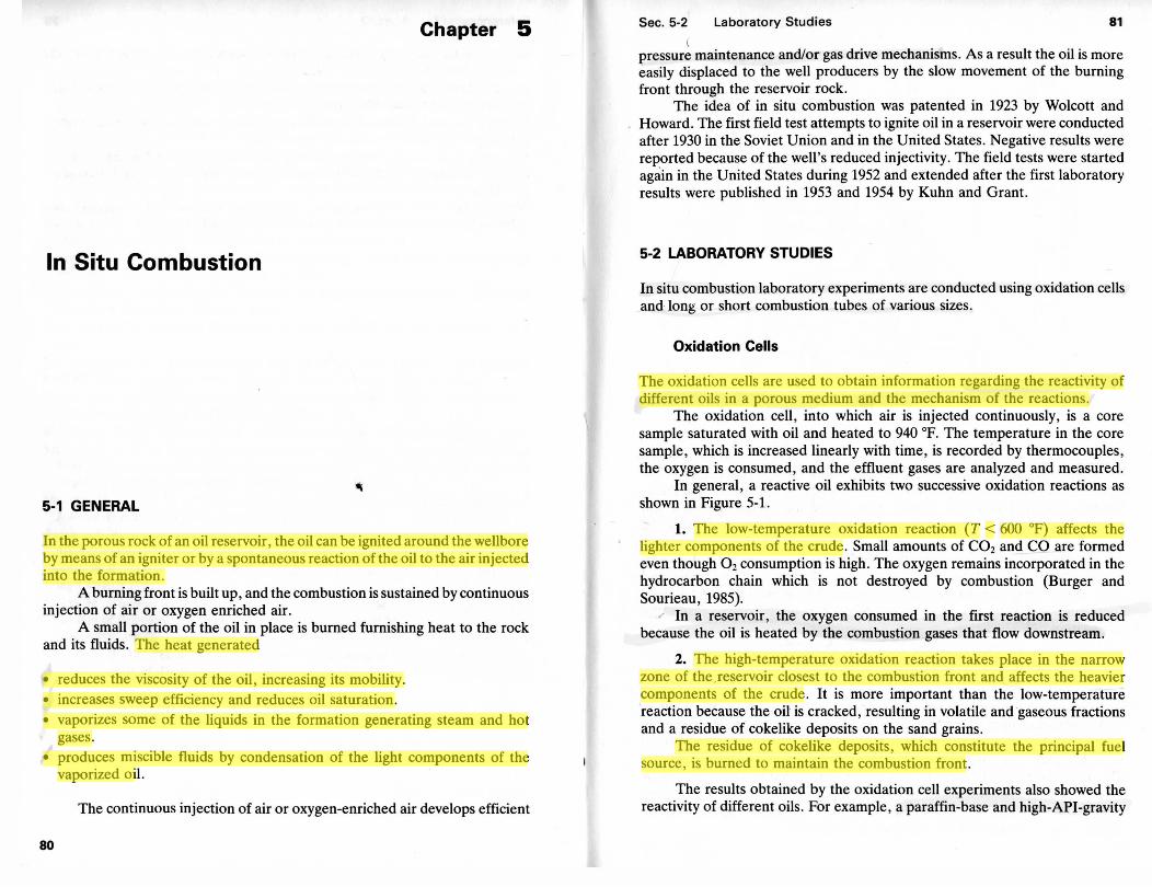
Chapter 5
In Situ Combustion
5-1 GENERAL
In the porous rock of an oil reservoir , the oil can be ignited around the well bore by means of an igniter or by a spontaneous reaction of the oil to the air injected into the formation .
A burning front is built up, and the combustion is sustained by continuous injection of air or oxygen enriched air.
A small portion of the oil in place is burned furnishing heat to the rock and its fluids. The heat generated
• reduces the viscosity of the oil, increasing its mobility. • increases sweep efficiency and reduces oil saturation. • vaporizes some of the liquids in the formation generating steam and hot
gases. • produces miscible fluids by condensation of the light components of the
vaporized oil.
The continuous injection of air or oxygen-enriched air develops efficient
80
Sec. 5-2 Laboratory Studies 81
(
pressure maintenance and/or gas drive mechanisms. As a result the oil is more easily displaced to the well producers by the slow movement of the burning front through the reservoir rock.
The idea of in situ combustion was patented in 1923 by Wolcott and Howard. The first field test attempts to ignite oil in a reservoir were conducted after 1930 in the Soviet Union and in the United States. Negative results were reported because of the well's reduced injectivity. The field tests were started again in the United States during 1952 and extended after the first laboratory results were published in 1953 and 1954 by Kuhn and Grant.
5-2 LABORATORY STUDIES
In situ combustion laboratory experiments are conducted using oxidation cells and· long or short combustion tubes of various sizes.
Oxidation Cells
The oxidation cells are used to obtain information regarding the reactivity of different oils in a porous medium and the mechanism of the reactions.
The oxidation cell , into which air is injected continuously, is a core sample saturated with oil and heated to 940 oF. The temperature in the core sample, which is increased linearly with time, is recorded by thermocouples, the oxygen is consumed, and the effluent gases are analyzed and measured.
In general , a reactive oil exhibits two successive oxidation reactions as shown in Figure 5-1.
1. The low-temperature oxidation reaction (T < 600 °F) affects the lighter components of the crude. Small amounts of C02 and CO are formed even though 0 2 consumption is high. The oxygen remains incorporated in the hydrocarbon chain which is not destroyed by combustion (Burger and Sourieau, 1985).
·' In a reservoir , the oxygen consumed in the first reaction is reduced because the oil is heated by the combustion gases that flow downstream.
2. The high-temperature oxidation reaction takes place in the narrow zone of the_reservoir closest to the combustion front and affects the heavier components of the crude. It is more important than the low-temperature reaction because the oil is cracked, resulting in volatile and gaseous fractions and a residue of cokelike deposits on the sand grains.
The residue of cokelike deposits , which constitute the principal fuel source , is burned to maintain the combustion front .
The results obtained by the oxidation cell experiments also showed the reactivity of different oils. For example , a paraffin-base and high-API-gravity
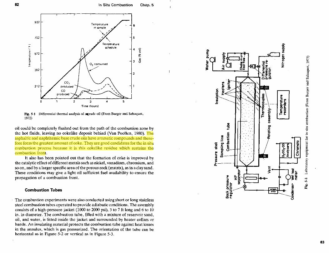
82
-.... ., :; :;; ~ C> E .,
,....
932
752
572
392
212
0 2 3
Time (hours)
In Situ Combustion Chap. 5
6
5
Temperature schedule
4 0 >
~ "' 3 ..
(,!)
2
4 5
Fig. 5-1 Differential thermal analysis of ~rude oil (From Burger and Sahuquet, 1972)
oil could be completely flushed out from the path of the combustion zone by the hot fluids, leaving no cokelike deposit behind (Van Poollen, 1980). The asphaltic and naphthemic base crude oils have aromatic compounds and therefore form the greatest amount of coke. They are good candidates for the in situ combustion process because it is this cokelike residue which sustains the combustion front.
It also has been pointed out that the formation of coke is improved by the catalytic effect of different metals such as nickel, vanadium, chromium, and so on, and by a larger specific area ofthe porous rock (matrix), as in a clay sand. These conditions may give a light oil sufficient fuel availability to ensure the propagation of a combustion front.
Combustion Tubes
The combustion experiments were also conducted using short or long stainless steel combustion tubes operated to provide adiabatic conditions. The assembly consists of a high-pressure jacket (1000 to 2000 psi), 3 to 7ft long and 6 to 10 in. in diameter. The combustion tube, filled with a mixture of reservoir sand, oil, and water, is fitted inside the jacket and surrounded by heater collars or bands. An insulating material protects the combustion tube against heat losses in the annulus, which is gas pressurized. The orientation of the tube can be horizontal as in Figure 5-2 or vertical as in Figure 5-3.
c.. E ~ c.. L. u -0 ~
f ~
"' "''cuo '--0.._2 .... ~ uoo ou alL
"" Q. c.. ~
"' c: ... Cl' 0 '-~
,;\ f
1-:.- tj c.. ::0 ~u ~ E 1- c.. ..... u
= 0
Cl' c: ·~
i ii'--... --u ~E
,-.. <""> t-0\ ...... ., ::s r::r ::s
..c:: 0: r/l
"0 c 0: .... 0) Oil .... ::s
a:l
e 0 e c:: 0
·;::
"' ::s ,D
E 0 u
. .§ "' .5 .... .£ ::: 0)
e ·~ r::r 0)
>, ....
~ .... 0
,D 0:
....)
~ Ill
oil r;
83

84
lnline Flow Transducer
Inlet Gas _ __.. _ __.
r-----1 I I
Electro ¢ Pneumatic Transducer
Effluent Gas
I
Back Pressure Regulator
Pneumatic Control Valve
.. .
In Situ Combustion
Solenoid Valve
Chap.5
Fig. S-3 Flow diagram for the automated in situ combustion assembly (From
Vossoughi and Willhite, 1982)
In the horizontal combustion tube system, to avoid gravitational segregation effects, the pressure jacket can be supported on steel rollers that enable the cell to rotate. After the ignition of the crude oil, air is inject_ed to sustain the combustion front. ,The exhaust gases are measured and analyzed continuously, the oil and water produced are separated, and t~eir p:o.d~c~ion history is determined. ·In-the vertical combustion tube orientatiOn, au 1s mJected from the top and all the effluerlts exit from the bottom of the ~ube.
The laboratory experiments, field tests, and commerctal developments of in situ combustion contributed to a better qualitative description of the process.
5-3 QUALITATIVE DESCRIPTION OF IN SITU COMBUSTION
The mechanism of oil displacement by a combustion front is complex. On a cross section made between an injection well and a producer in a reservoir formation with uniform permeability, the combustion front has practically an elongated S shape. The density differences between injected air and reservoir
Sec. 5-3 Qualitative Description of In Situ Combustion 85
liquids make evident the gravitational segregation and the tendency of gas to override (Figure 5-4). . This tendency is accentuated when the reservoir thickness is larger atld 1s attenuated when the formation is inclined. Under steady-state conditions the various zones formed in the reservoir during the in situ combustion process are as follows:
Zone 1
Zone2
Zone3
Zone 4
is the combustion front, where the oxygen is consumed in burning the coke deposited on rock grain surfaces and steam is one of the products formed. Zone 1 has the highest temperature, from 600 to 1200 oF.
is left behind by the combustion front as a hot and clean sand that heats the injected air before the air reaches the front. is the vaporization zone ahead of the combustion front, where the lighter hydrocarbons and the interstitial water are vaporized and the heavier hydrocarbons are thermally cracked, leaving the cokelike deposit on the sand grains. is the condensation zone where the steam and the hydrocarbon gases move forward into the cooler reservoir, condense, and a large amount of heat is released. The oil displacement is increased by the oil's lower viscosity, higher mobility, and the miscible effect of the mixture between the condensed gas and the oil bank.
Air Injection
[D Combustion Front
0 Burned Rock
~Vapor Zone
Producer
~ Condens,Zone
CIJ Oil Bank
4
. ·.:. ·rn -~· . .. ·.· .. ·4'·:··:.-.
. . .. . . . . . . . .
Fig. S-4 Schematic representation of in situ combustion process and the various zones as formed in the oil reservoir
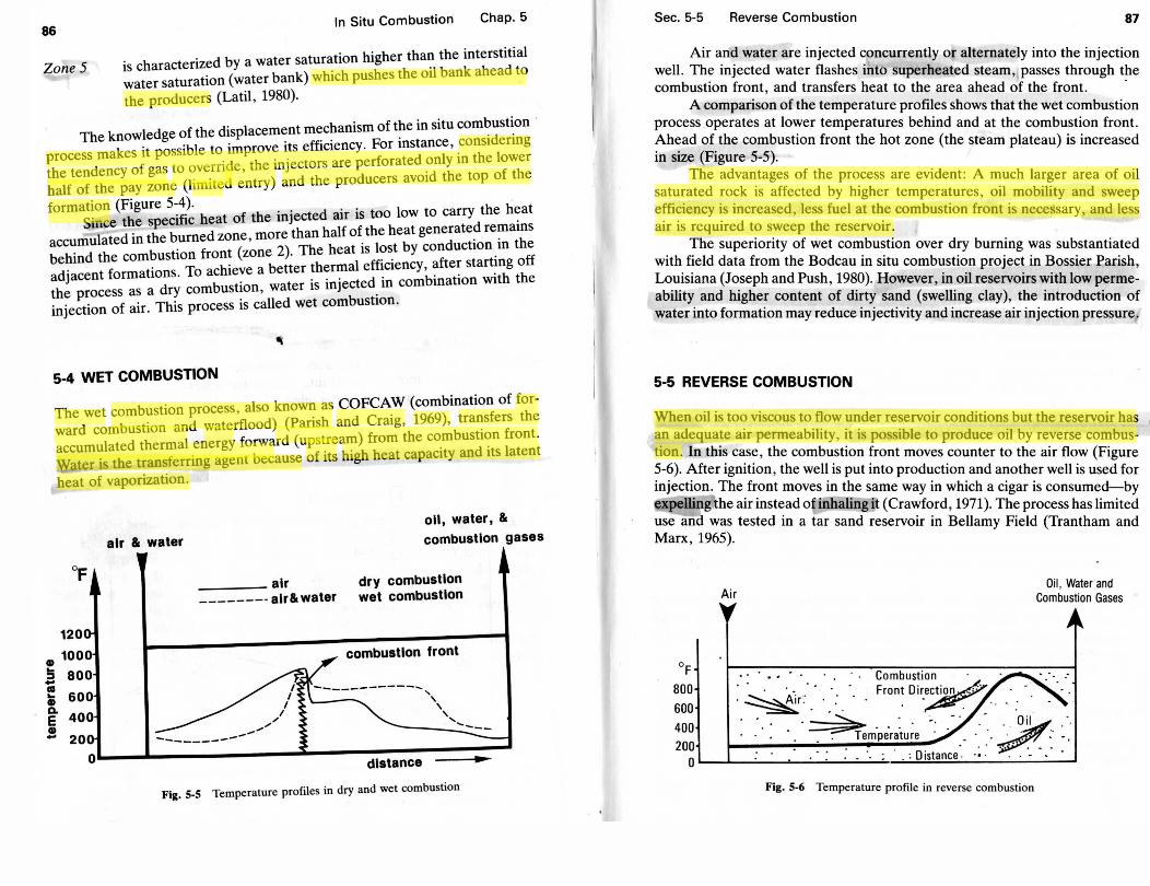
86
ZoneS
In Situ Combustion Chap. 5
. d by a water saturation higher than the interstitial ~:~~r:~~:~~~on (water bank) which pushes the oil bank ahead t_o
the producers (Latil , 1980).
h dis lacement mechanism of the in situ combustion . The know~edge ~f t e . p rove its efficiency. For instance, considering
process makes lt possible to.:;npthe injectors are perforated only in the lower the tendency of gas to(l~ve_rtn d e~ntry) and the producers avoid the top of the half of the pay zone lml e
format~on (F~gure 5~:;~ heat of the injected air is too low to carry the h:at Smce t . e specl ore than half of the heat generated remams
accumulated m the b_urned zont m 2) The heat is lost by conduction in the be~ind tht cori~?ustlO;of:~~~e::~~et~er thermal efficiency, after start~ng off adJacent orma wdns. b fan water is injected in combination Wlth the the process as a ry com us 1 ' .
injection of air. This process is called wet combustwn.
5-4 WET COMBUSTION
COFCAW (combination of forThe wet comb~stion ~rocetssrll~~~~(~:r~s~s and Craig, 1969), transfers the ward combustwn an wa e rd (u stream) from the combustion front. accumulated thermal _energy forwb a ~fits high heat capacity and its latent Water is he transfernng agent ecause heat of vaporization .
120
., 100 !5 800 ... CD ... ., a. E !
air & water
____ air
--------air& water
oil, water, & combustion gases
dry combustion wet combustion
combustion front
distance
Fig. 5-S Temperature profiles in dry and wet combustion
Sec. 5-5 Reverse Combustion 87
Air and water are injected concurrently or alternately into the injection well. The injected water flashes into superheated steam, passes through the combustion front, and transfers heat to the area ahead of the front. -
A comparison of the temperature profiles shows that the wet combustion process operates at lower temperatures behind and at the combustion front . Ahead of the combustion front the hot zone (the steam plateau) is increased in size (Figure 5-5).
The advantages of the process are evident: A much larger area of oil saturated rock is affected by higher temperatures, oil mobility and sweep efficiency is increased, less fuel at the combustion front is necessary, and less air is required to sweep the reservoir.
The superiority of wet combustion over dry burning was substantiated with field data from the Badeau in situ combustion project in Bossier Farish, Louisiana (Joseph and Push, 1980). However, in oil reservoirs with low permeability and higher content of dirty sand (swelling clay), the introduction of water into formation may reduce injectivity and increase air injection pressure.
5-5 REVERSE COMBUSTION
When oil is too viscous to flow under reservoir conditions but the reservoir has an adequate air permeability, it is possible to produce oil by reverse combustion. In this case , the combustion front moves counter to the air flow (Figure 5-6). After ignition, the well is put into production and another well is used for injection. The front moves in the same way in which a cigar is consumed-by x lling the air instead of inhaling it (Crawford, 1971 ). The process has limited
use and was tested in a tar sand reservoir in Bellamy Field (Trantham and Marx, 1965).
Air Oil , Water and
Combustion Gases
OF
800 600 400 200 OL-~--~--_.~~~~·~·~· ~:~-· ~-~: ~O~is~ta~n~ce~-------------~
Fig. S-6 Temperature profile in reverse combustion
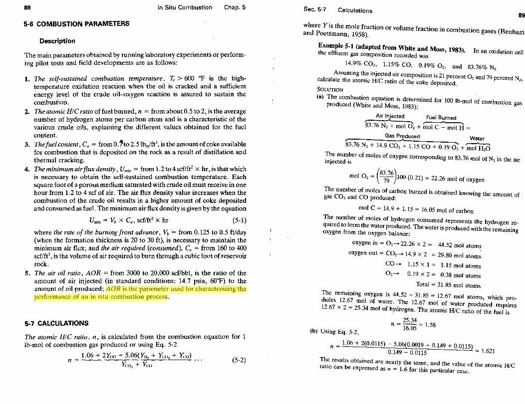
88 In Situ Combustion Chap. 5
5-6 COMBUSTION PARAMETERS
Description
The main parameters obtained by running laboratory experiments or performing pilot tests and field developments are as follows:
1. The self-sustained combustion temperature, 'Fe > 600 op is the hightemperature oxidation reaction when the oil is cracked and a sufficient energy level of the crude oil-oxygen reaction is assured to sustain the combustion.
2. The atomic H/C ratio offuel burned, n = from about 0.5 to 2, is the average number of hydrogen atoms per carbon atom and is a characteristic of the various crude oils, explaining the different values obtained for the fuel content.
3. The fuel content, Cu = from 0. 1to 2. 5 lbm/ft3, is the amount of coke available
for combustion that is deposited on the rock as a result of distillation and thermal cracking.
4. The minimum air flux density, Umin = from 1.2 to 4 scf/ftz x hr, is that which is necessary to obtain the self-sustained combustion temperature. Each square foot of a porous medium saturated with crude oil must receive in one hour from 1.2 to 4 scf of air. The air flux density value increases when the combustion of the crude oil results in a higher amount of coke deposited and consumed as fuel. The minimum air flux density is given by the equation
Umin = vb X c., scf/ft2 X hr (5-1)
where the rate of the burning front advance, Vb ~from 0.125 to 0.5 ft/day (when the formation thickness is 20 to 30ft), is necessary to maintain the minimum air flux; and the air required (consumed), c. = from 160 to 400 scf/ft3
, is the volume of air required to burn through a cubic foot of reservoir rock.
5. The air oil ratio, AOR = from 3000 to 20,000 scf/bbl, is the ratio of the amount of air injected (in standard conditions: 14.7 psia, 60op) to the amount of oil produced; AOR is the parameter used for characterizing the performance of an in situ combustion process.
5-7 CALCULATIONS
The atomic HJC ratio, n, is calculated from the combustion equation for 1 lb-mol of combustion gas produced or using Eq. 5-2
1.06 + 2Yco - 5.06(Yo2 + Yco2 + Yeo) n = ... Ycaz +Yeo
(5-2)
Sec. 5-7 Calculations 89
whderpe y is the mole fraction or volume fraction in combustion gases (Benham an oettmann, 1958).
Example 5-1 (adapted from White and Moss 1983) the effluent gas composition recorded was ' • In an oxidation cell
14.9% COz, 1.15% CO, 0.19% Oz, and 83.76% Nz
al I Assuming th~ injected air composition is 21 percent Oz and 79 percent N c cu ate the atomic H/C ratio of the coke deposited. 2
'
SOLUTION
(a) The combustion equation is determined for 100 lb-mol of comb f produced (White and Moss, 1983): us Ion gas
Air Injected Fuel Burned , ...... "~ 83.76 Nz +mol 0 2 +mol c +mol H =
, Gas Pr~duced Water
83.76 Nz + 14.9 C02 + 1.15 CO+ 0.19 0~ +mol H20
~e num.ber of moles of oxygen corresponding to 83.76 mol of N in th · InJected IS z e au
mol 0 = (83.76) 2 79 100 (0.21) = 22.26 mol of oxygen
TheCnOumber of moles of carbon burned is obtained knowing the amount of gas z and CO produced:
mol C = 14.9 + 1.15 = 16.05 mol of carbon
Th~ number of moles of hydrogen consumed represents the h dro en required to form the water produced. The water is produced with th~ re~ainin oxygen from the oxygen balance: g
oxygen in = Oz~ 22.26 X 2 = 44.52 mol atoms
oxygen out= COz~ 14.9 x 2 = 29.80 mol atom~
CO~ 1.15 X 1 = 1.15 mol atoms
Oz~ 0.19 X 2 = 0.38 mol atoms
Total = 31.85 mol atoms
The remaining oxygen is 44.52 - 31 85 = 12 67 1 h' d · 12 6 · · mo atoms, w Ich pro-1~ces . ! mol of water. The 12.67 mol of water produced requires
.67 x 2 - 25.34 mol of hydrogen. The atomic H/C ratio of the fuel is
(b) Using Eq. 5-2,
25.34 n = 16.05 = l.S8
n = 1.06 + 2(0.0115) - 5.06(0.0019 + 0.149 + 0.0115) 0.149 0.0115 = 1.621
:~~ resul~ obtained are nearly the same, and the value of the atomic H/C a to can e expressed as n = 1.6 for this particular case.
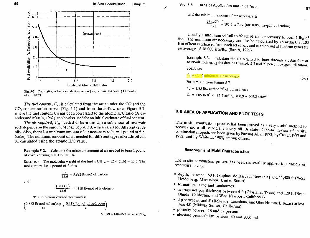
90 In Situ Combustion Chap. 5
_, (.)
0 a: 6.0 .... E ::l
co ..... 0
.... ..... :::i (.)
c 0
-e "' (.)
:e > ~ :.c
1\ Ottawa Sand
~ 0
~ . 0
~
5.0
4.0
3.
2
~ ·;;; :>
<(
.0 It
a; ::l
u.. 0
2. 1.5 1.6 1. 7 1.8 1.9 0 Crude 0 il Atomic H/C Ratio
Fig. S-7 Correlation of fuel availability (content) with atomic H/C ratio (Alexander et a!., 1962)
The fuel content, Cu, is calculated from the are~ under the C? and the C02 concentration curves (Fig. 5-1) and from the mrflo~ rate. Ft~re 5-7,
here the fuel content Cu has been correlated to the atomic H/C ratio (Alex:nder and Martin, 1962), can be also used for an initial esti~ate of fuel conten~.
T.h · uz'red c needed to burn through a cubic foot of reservoir e azr req , "' · f d'ff t d k depends on the amount of coke deposited, which vanes or I eren cru e
r~c h . . . m amount of air necessary to burn 1 pound of fuel oils Also t ere IS a mmimu .1 (coke). The minimum amoun~ of air needed for different types of crude 01 can
be calculated using the atomic H/C value.
Example 5-2. Calculate the minimum amount of air needed to burn 1 pound of coke knowing n = H/C = 1.6.
· f h fu 1 · CH = 12 + (1.6) = 13.6. The SOLUTION The molecular wetght o t e e ts 1.6
mol content for 1 pound of fuel is
and
_Q_ = 0.882 lb-mol of carbon 13.6
1 x (1.6) = 0.118 lb-mol of hydrogen 13.6
The minimum oxygen necessary is
(0.882 lb-mol of carbon + 0.118 lb-mol of hydrogen)
12 4
x 379 scf/lb-mol = 39 scf!lbm
I Sec. 5-8 Area of Application and Pilot Tests
91
and the minimum amount of air necessary is
39
0~~~lb = 185.7 scf!lbm (for 100% oxygen utilization)
Usually a minimum of 160 to 92 scf of air is necessary to burn 1 lbm of fuel. The minimum air necessary can also be calculated by knowing that 100 Btu of heat is released from each scf of air, and each pound of fuel can generate an average of 18,000 Btu/Ibm (Smith, 1985).
Example 5-3. Calculate the air required to burn through a cubic foot of reservoir rock using the data of Example 5-2 and 90 percent oxygen utilization .
SOLUTION
C. = Cu x minimum air necessary (5-3)
For n = 1.6 from Figure 5-7
Cu = 1.85 Ibm carbonlfe of burned rock
c. = 1.85 lb!fe x 185.7 scf!lbm x 0.9 = 309.2 scflfe
5-8 AREA OF APPLICATION AND PILOT TESTS
The in situ combustion process has been proved as a very useful method to recover more oil, especially heavy oil. A state-of-the-art review of in situ combustion projects has been given by Farouq Ali in 1972, by Chu in F/77 and 1982, and by White in 1985, among others.
Reservoir and Fluid Characteristics
The in situ combustion process has been successfully applied to a variety of reservoirs having
• depth, between 160ft (Suplacu de Barcau, Romania) and 11,400 ft (West Heidelberg, Mississippi, United States)
• formations, sand and sandstones
• average net pay thickness between 4ft (Gloriana, Texas) and 120ft (Brea Olinda, California, and West Newport, California)
• dip between 0 and 5° (Bellevue, Louisiana, and Glen Hummel, Texas) or less than 45° (Midway Sunset, California)
• porosity between 16 and 37 percent • absolute permeability between 40 and 8000 md

92 In Situ Combustion Chap. 5
The majority of in situ combustion field projects have been conducted in reservoirs with heavy crude oil, between 15 and 22 API, and viscosities b~twe~o 10 and 6000 cp at reservoir temperature. There are also successf~l proJect~ 1? light oil reservoirs with viscosities less than 10 cp sue~ as May-Ltbby, Lom~tana, with 3 cp, or Sloss, Nebraska, with 0.8 cp (Parnsh, Pollock, and Cratg, 1974). . .
The in situ combustion method can also be used for very vtscous olls or for tar sand reservoirs. In these formations, to obtain an acceptable pressure level and oil mobility, the process must be combined with fracturing techniques and steam stimulation.
Regarding the reservoir oil saturation at the start of the process, the values vary between 30 percent at ~loss, Nebraska, and 94 percent at East Tia Juana, Venezuela. An oil saturation of 30 to 40 percent at the start of the process means that the reservoir has been waterflooded previously or has bee? produced by cyclic steam and/or steam drive (Counihan, 1977). A va.lue of ml saturation higher than 85 percent (for example, 94 percent-East Tta Juana, Venezuela) shows an oil-wet rock reservoir.
In the life of a reservoir, the in situ combustion process can be applied:
• as the primary method for developing production Of a heavy oil reservoir without natural oil mobility characteristics.
• as a secondary method, after the natural depletion of reservoir. • as a tertiary method, after waterflooding or cyclic steam and/or steam drive
operations.
Pilot Tests
Prior to field development of in situ combustion, pilot tests involving a small portion of the reservoir are conducted in order to check the laboratory results and to obtain
• data to design surface injection facilities (injection pressure, injection rate). • information regarding formation damage, sand invasion, emulsions, corro
sions, and so on. • data about the existence of preferential fluid flow, directional permeabili
ties, gas fingering , impermeable barriers, and so on. • production rates, temperatures, and effluent gas measurements; burning
front configuration and velocity, and so on. • information regarding the oil recovery (only if the field pilot is considered
a confined pattern).
The conventional pattern for most pilots is the inverted five-spot array with one injector in the middle and four producers in the corners of a square (Figure 5-8a).
I
L
Sec. 5-8 Area of Application and Pilot Tests
(a)
r-, I fl I
, .__~
~lnj.Well e Producer
u
(b)
-I, 12
'/---~ I • I I I
13k.-- _J, 14 -
Fig. 5-8 Open inverted (a) and confined direct (b) five-spot
93
4
If the combustion is performed in four adjacent inverted five-spot patterns with injection wells I~> lz, l3, and 14 (Figure 5-8b ), the four injection wells then encompass a direct five-spot pattern which may be considered a confined pattern with a central production well P.
The cumulative oU production of the well P divided to the initial oil in place, corresponding to the direct five-spot pattern area, gives an estimate of the oil recovery.
Example 5-4. A combustion test in a confined pattern was conducted on a depleted oil reservoir with a current oil recovery of 10 percent . Estimate the final oil recovery expected after the commercial development of the in situ coml!mstion method, given the following:
Confined area
Net thickness
Effective porosity
Irreductible water saturation
Oil formation volume factor Initial Current
Cumulative oil production of the central well P, as the effect of combustion
SOLUTION The initial oil in place is given by
N = 7758<1>(1 - Sw;) Ax h Boi
1.25 acres 20ft
24%
25%
1.12 1.05
flNc = 12,470 bbl
N = 7758 ~ x (0.24)(0.7S) 1.25 acres x 20ft acre-ft 1.12
N = 31,170 bbl of oil
(5-4)

94 In Situ Combustion · Chap. 5
The increase in oil recovery as the result of in situ combustion is
= f1Nc = 12,470 = 0.40 or 40% ERe N 31 ,170
The final oil recovery expected is
0.10 + 0.40 = 0.50 or
After the evaluation oftthe pilot test results , implementation of in situ combustion is expanded using different flood patterns.
-9 FIELD DEVELOPMENT
The expansion of the in situ combustion p~ocess. to full sc~le ~ay use well patterns based on the five-spot or staggered hne dr~~e wh_en duect10nal perm~abilities are known to exist. Existing wells are utlhzed tf the old wells_ are m good working order. New injection and production wells have fo be dnlle? as
well. · · · 0 Basically, the in situ combustion process i~ simil~r to gas InJeCtiOn. . ne
of the most important factors to be considered 1s the mfluence of the gravita-tional effect on the flow of fluids . . .
In Figure 5-9a, Well 1 will produce more ml at htgh~r rates because. of a slightly isobatic difference. In Figure 5-9b, the combustl?n. g~s. segre~at10n upward is accentuated as the formation dip incre~ses and au 1s InJected m ~he higher regions. Also , the air's tenden~y to over_nde the top of the formatiOn is diminished and the oil flows downdtp where 1t can be produced at a lower air-oil ratio and at higher rates.
(a) (b)
' Fig. 5-9 Gravitational effect on the fluids flow in an in situ combustion process
Sec. 5-9 Field Development 95
For this reason combustion operations in dip reservoirs should start , upstructure , at the uppermost part of the reservoir, and progress downward.
Where large gas caps exist , combustion operations have to be avoided or started down the structure. For flat reservoirs , where the injected air will not move updip, uni~orm well patterns with central injection wells are used .
The main characteristics and results of in situ combustion projects are presented th~o~gh three examples of field applications. The Moco Zone project, in California, was one of the first commercial in situ combustion processes initiated. The Suplacu de Barcau Field, Romania, is the largest developed process known. The Heidelberg Field, Mississippi , is the deepest applied process.
The Moco Zone, California, United States
The Moco Zone project is one of the Midway Sunset fields in California (Gates and Sklar, 1985).
\
Characteristics. The reservoir is an anticline at a depth of 2100-2700 feet. The six major sands of the pay zone have 129 feet total net thickness and are inclined up to 45° to the north and zoo to the south (Figure 5-10).
The heavy crude oil in this reservoir has 14.5 °API gravity and 110 cp viscosity at reservoir temperature . The ultimate oil recovery under natural depletion was estimated at 17 percent Considering the gravitational effect and the pay zone's high specificp ermeabili y of 1575 md, the above ref overy value is possible and could even be exceeded if the reservoir is produced for an extended period.
Performances. Combustion was initiated in 1960 by spontaneous ignition after about 18 days of air injection in a well located high in the structure. As the process was continued the combustion front formed and moved downward on the flanks of the anticline. After 10 years the total air injection rate into five injectors was about 6000 Mcf/day and the oil rate from 30 producers was 1600 bbl/day. The cumulative air-oil ratio was 2890 scf/bbl and the oil recovery r~ached at the same time was 24 percent of the initial oil in place.
Experience. As one of the first in situ combustion processes successfully operated, this project provided useful experience regarding results and operating conditions.
• After the compressor capacity reaches the projected injection rate, any decrease of this rate corresponds with an oil rate decline.
• The pressure that forms in the secondary gas cap high in the structure as a result of the presence of combustion gas and air has to be kept constant , with no leakage to the adjacent formations or through old wells.

96 In Situ Combustion Chap.5
504-35
(a) Structure
504 95 86 1,000 It
2.000 It
0 1,000
(b) Cross section E-E' It
Fig. 5-10 Moco Zone structure and cross section showing centrally located injection wells (From Gates and Sklar, 1985)
Sec. 5-9 Field Development 97
• Any increase in the air injection rate means more fluid displacement downdip, which must be sustained with improved well capacity rates or with more production wells.
• Low air-oil,rratio and high oxygen efficiency for the wells located downstructure is due to the gravitational effect.
• Spontaneous ignition may take place not at the formation face near the wellbore but in the formation a short distance from the well. In this case the liner_ or the well casing can be damaged by the back movement of the burning
. front. For this reason cemented and perfor'ated liner-installation is recom- >
mended. • Sand invasion is prevented by the classic method of gravel packing. • The bottom hole temperatures ought to be measured frequently at the
producers~· Hot temperatures have to be prevented by injecting cooling water into the tubing-casing annulus.
Suplacu de Barcau, Romania
Suplacu de Barcau field , situated in northwestern Romania, is the world's largest in situ combustion process (Carcoana et al., 1976, 1983, 1990; Gadelle et al. , 1981).
Characteristics. ·The shallow oil reservoir of Suplacu de Barcau (164-to 656-ft depth) consists of slightly shaley unconsolidated average to coarse sands with 0.32 porosity and 1700 to 2000 md permeability. The reservoir, an east-west monocline with 2 to 7° dip north has a net pay thickness of 33 feet and an original oil in place reserve of 295 MM bbl. A general view of the field is shown in Figure 5-11. The central part of the zone subjected to combustion
0 1 ........ Miles I ••••••• tl
.•• • •• I • ••• • I • • • • • • I ""'"/
\ r// • /1_..../ . _,.../
..... , --/
/
e e e Oil Water Contact
---Faults
Fig. 5-11 Suplacu de Barcau field (From Carcoana, 1990)
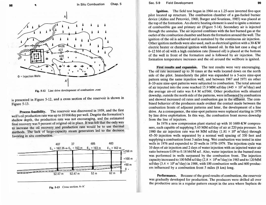
98 In Situ Combustion Chap. 5
·' . /
A'l Fig. S-12 Line drive development of combustion ,ront
is presented in Figure 5-12, and a cross section of the reservoir is shown in
Figure 5-13.
Process feasibility. The reservoir was discovered in ~959 , and the.fir~t well's oil production rate was up to 10 bbl/day per well . J?ewtte the forrn~twn s shallow depth , the production rate was not encouragmg, and the esttmated final recovery was 9 percent of original oil in place. It was felt that the only way to increase the oil recovery and production rate would be to use the~~al methods . The lack of large-capacity steam generators led to the declSlon favoring in situ combustion.
407 37 485 483
----------------E:L~=J16~2~. 3~5~m~E~Lr=-1_63 __ m===E:L==r1=6=3=m====E=L~~=1=6=2=m~==========~----~----~--------1-------ij---;t-+150m
! +100m _1
,
------------------~~-----ir--------1--------ii--~J~+'50m
. . . . . .. ·· .· .-·.:: · ., ,·· .: :.:.;:; : '·'' ' ' ·' :~ ... 2~ ~:; ' ' ·:::.:.:.: ·.': :·~. ~:. :.-. :. : ::·.J) ':L~ .J·~Li:;·2::t: .:;:24 o. ;,:. .. :.:.:;.:;..:~ ·. ·. ···- 52.47 m 52.47 m 52 m 62 m I
Fig. 5-13 Cross section A-A'
Sec. 5-9 Field Development 99
Ignition. The field test began in 1964 on a 1.25-acre inverted five-spot pilot located up structure. The combustion chamber of a gas-fueled burner device (Aldea and Petcovici , 1968; Burger and Sourieau, 1985) was placed at the top of the formation . An electric heating element is used to ignite a mixture of q>mbustible gas and primary air (Figure 5-14). Secondary air is injected through the annulus . The air injected combines with the hot burned gas at the outlet of the combustion chamber and heats the formation around the well . The ignition of the oil is achieved and is sustained by the continuous air injection . Other ignition methods were also used , such as electrical ignition with a 30-KW electric 'heater or chemical ignition with linseed oil. In this last case a slug of 6-12 bbl of oil with a high oxidation rate (linseed oil) is placed at the bottom of the well in front of the formation and is followed by air injection . The formation temperature increases and the oil around the wellbore is ignited .
First results and expansion. The test results were very encouraging . The oil rate increased up to 30 times at the wells located down on the north side of the pilot. Immediately the pilot was expanded to a 5-acre nine-spot pattern using the same injection well , and between 1967 and 1971 six other 8-10-acre nine-spot patterns were subjected to combustion. The total amount of air "injected into the zone reached 15 .9 MM scf/day (445 x 103 m3/day) and the average air-oil ratio was 8.4 M scf/bbl. Other production wells situated down dip , outside the north side of the patterns, were influenced by combustion and showed increased oil rates and combustion gas in the effluent. The combined behavior of the producers made ev,ident the contact made between the combustion fronts of adjacent patterns and later, (he development of a line drive. As a conseq1.:1ence, the nine-spot patterns were replaced starting in 1970 by line drive exploitation. In this way, the combustion front moves downdip from the line of injectors.
In 1976 a new compression plant started up with 10 1600-KW compressors, each capable of supplying 5.65 MM scf/day of air at 220 psia pressure. In 1980 the air injection rate was 64 MM scf/day (1.81 x 10⁶ m3/day) through 45-50 injection wells separated by a normal well spacing of 330 feet and supplying· a combustion front 3 miles long. Wet combustion was tested in nine wells in 1976 and expanded to 20 wells in 1978-1979. The injection cycle was 10 days of air injection and 2 days of water injection with an injected water-air ratio between 0.09 to 0.18 bbl/M scf. Also, water injection in the burned zone was performed in wells surpassed by the combustion front. The injection capacity increased to 100 MM scflday (2.8 x 10⁶ m3/day) in 1983 and to 120 MM scf/day (3.4 x 10⁶ m3/day) in 1988, with\ 100 combustion wells and 600 producers influenced by a combustion front 5 miles (8 km) long.
Performance. Because of the good results of combustion, the reservoir was gradually developed for production. The producers were drilled all over the productive area in a regular pattern except in the area where Suplacu de
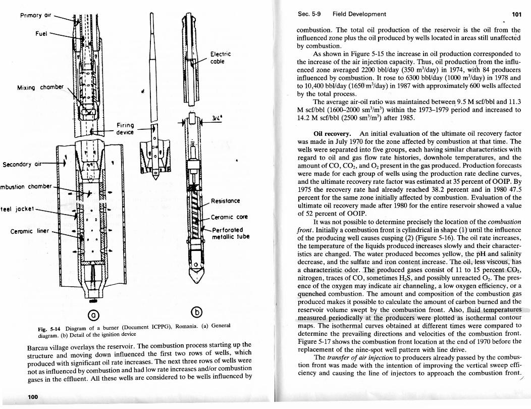
Pnmary air
MixinQ chamber
mbustion chamber
teel jacket
0
Ceramic liner
•
Firing ~--device
,
•
• ... 0
... •
• •
Electric cable
&
Resistance
Ceramic core
Perforated metallic tube
Fig. 5-14 Diagram of a burner (Document ICPPG), Romania . (a) General diagram. (b) Detail of the ignition device
Barcau village overlays the reservoir . The combustion process starting up ~he structure and moving down influenced the first two rows of wells, wh1ch produced with significant oil rate increases. The ~ext three rows of wells w~re not as influenced by combustion and had low rate mcreases and/~r combustiOn gases in the effluent. All these wells are considered to be wells mfluenced by
100
Sec. 5-9 Field Development 101
combustion. The total oil production of the reservoir is the oil from the influenced zone plus the oil produced by wells located in areas still unaffected by combustion.
As shown in Figure 5-15 the increase in oil production corresponded to the increase of the air injection capacity. Thus, oil production from the influenced zone averaged 2200 bbl/day (350 m3/day) in 1974, with 84 producers influenced by combustion. It rose to 6300 bbl!day (1000 m3/day) in 1978 and to 10,400 bbl/day (1650 m3/day) in 1987 with approximately 600 wells affected by the total process.
The average air-oil ratio was maintained oetwee~ 9.5 M scf/bbl and 11.3 M scf/bbl (1600-2000 sm3/m3
) within the 1973-1979 period and increased to 14.2 M scf/bbl (2500 sm3/m3
) after 1985.
Oil recovery. An initial evaluation of the ultimate oil recovery factor was made in July 1<rZO for the zone affected by combustion at that time. The wells were separated into five groups, each having similar characteristics with regard to oil and gas flow rate histories, downhole temperatures, and the amount of CO, C02 , and 0 2 present in the gas produced. Production forecasts were made for each group of wells using the production rate decline curves, and the ultimate recovery rate factor was estimated at 35 percent of OOIP. By 1975 the recovery rate had already reached 38.2 percent and in 1980 47 .5 percent for the same zone initially affected by combustion. Evaluation of the ultimate oil recovery made after 1980 for the entire reservoir showed a value of 52 percent of OOIP.
It was not possible to determine precisely the location of the combustion front . Initially & combustion front is cylindrical in shape (1) until the influence of the producing well causes cusping (2) (Figure 5-16). The oil rate increases, the temperature of the liquids produced increases slowly and their characteristics are changed. The water produced becomes yellow, the pH and salinity decrease, and the sulfate and iron content increase. The oil , less viscous, has a characteristic odor. The produced gases consist of 11 to 15 percent COz, nitrogen, traces of CO, sometimes H2S, and possibly unreacted 0 2• The presence of the oxygen may indicate air channeling, a low oxygen efficiency, or a quenched combustion. The amount and composition of the combustion gas produced makes it possible to calculate the amount of carbon burned and the reservoir volume swept by the combustion front. Also, fluid temperatures measured periodically at the producers were plotted as isothermal contour maps. The isothermal curves obtained at different times were compared to determine the prevailing directions and velocities of the combustion front . Figure 5-17 shows the combustion front location at the end of 1970 before the replacement of the nine-spot well pattern with line drive.
The transfer of air injection to producers already passed by the combustion front was made with the intention of improving the vertical sweep efficiency and causing the line of injectors to approach the combustion front.
/

102
0 0 0 0 N CO M N
.. ·. ··· ··;.•
0 0 0 0 """ 0 N N
0 0 0 0 0 0 0 0 CD N CO '<!" 0
·· ..
0 0 0 N
· .. ... ...
<. , ·~ ~ -.._ .,
-J==x+ ---=='-. --·-·-·,_.,. P/l ' ale~ poJd 1!0 a6eJaflv
0 0 0 0 ....., 0
0 0 0 0 0 0 0 0 ....., ....., ....., ....., M N
l/cWS 'O!le~ 1!0 J!V
....., • co
en
0 co
·en
....., ..... en
0 ..... en
-CD en
Sec. 5-9 Field Development
• Producer 4
/I / I
2 / I // I
/ I .,.,/ I
/
_..--;... __, I --/ ' I
'I '"~ \: \ I I
' / \ ..__ ,; Fig. 5-16 Initial shape of combustion front
103
Observation wells drilled in the burned zone showed that approximately the top half of the pay zone was burned, followed by a coke layer and below, the unburned oil saturated zone. For example, the cross section (Fig. 5-18a) illustrates the moment when the combustion front approaches producer "428." The temperature measured at well "428" is rising, the oil rate has a sharp exponential decline and hot combustion gases are produced. To avoid damages, well "428" has to be shut down, and wells "427" and "426" should be ready to produce the oil bank. As the combustion front advances, the distance between the line of injectors and the wells influenced by combustion increases. The approach of the injectors line was made by transferring air injection from well "14" to well "428" and so on (Figure 5-18b ). Air efficiency and vertical sweep efficiency were increased. The air injection was transferred directly, since the formation temperature was appropriate for spontaneous ignition to take place.
The oil recovery was checked systematically using detailed contour maps for the top and base of the formation (Machedon et al. , 1975). The original oil in place was calculated for each section of the reservoir between two isobaths from 10 to 10m (33ft). The cumulative oil produced by the wells in each section gives the recovery factor at any particular time (Figure 5-19). The flow of oil between sections takes place only downward, and the amount that leaves one section is produced through the wells of the section below.
Difficulties. One of the rna jor difficulties observed at the beginnin&\ was the leakage of combustion gases to the surface . Because formerly producing wells were unplugged or improperly sealed, leaking casings were acting as conduits for gas and/or steam to move to the surface . Mud and steam volcanoes
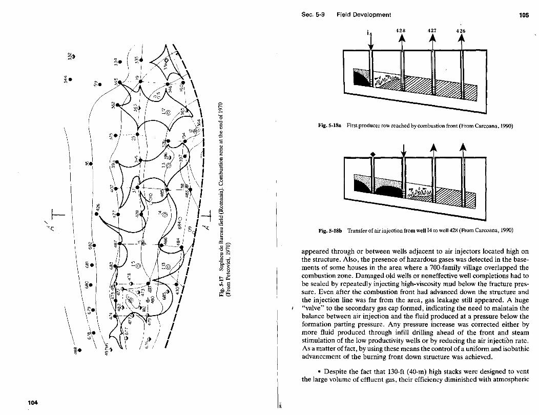
\ \ \
~-.,
104
Sec. 5-9 Field Development 105
428 427 426
Fig. 5-18a First producer row reached by combustion front (From Carcoana, 1990)
Fig. 5-18b Transfer of air injection from well 14 to well428 (From Carcoana, 1990)
appeared through or between wells adjacent to air injectors located high on the structure. Also, the presence of hazardous gases was detected in the basements of some houses in the area where a 700-family village overlapped the combustion zone. Damaged old wells or noneffective well completions had to be sealed by repeatedly injecting high-viscosity mud below the fracture pressure. Even after the combustion front had advanced down the structure and the injection line was far from the area, gas leakage still appeared. A huge "valve" to the secondary gas cap formed, indicating the need to maintain the balance between air injection and the fluid produced at a pressure below the formation parting pressure. Any pressure increase was corrected either by more fluid produced through infill drilling ahead of the front and steam stimulation of the low productivity wells or by reducing the air injection rate. As a matter offact, by using these means the control of a uniform and isobathic advancement of the burning front down structure was achieved.
• Despite the fact that 130-ft (40-m) high stacks were designed to vent the large volume of effluent gas, their efficiency diminished with atmospheric
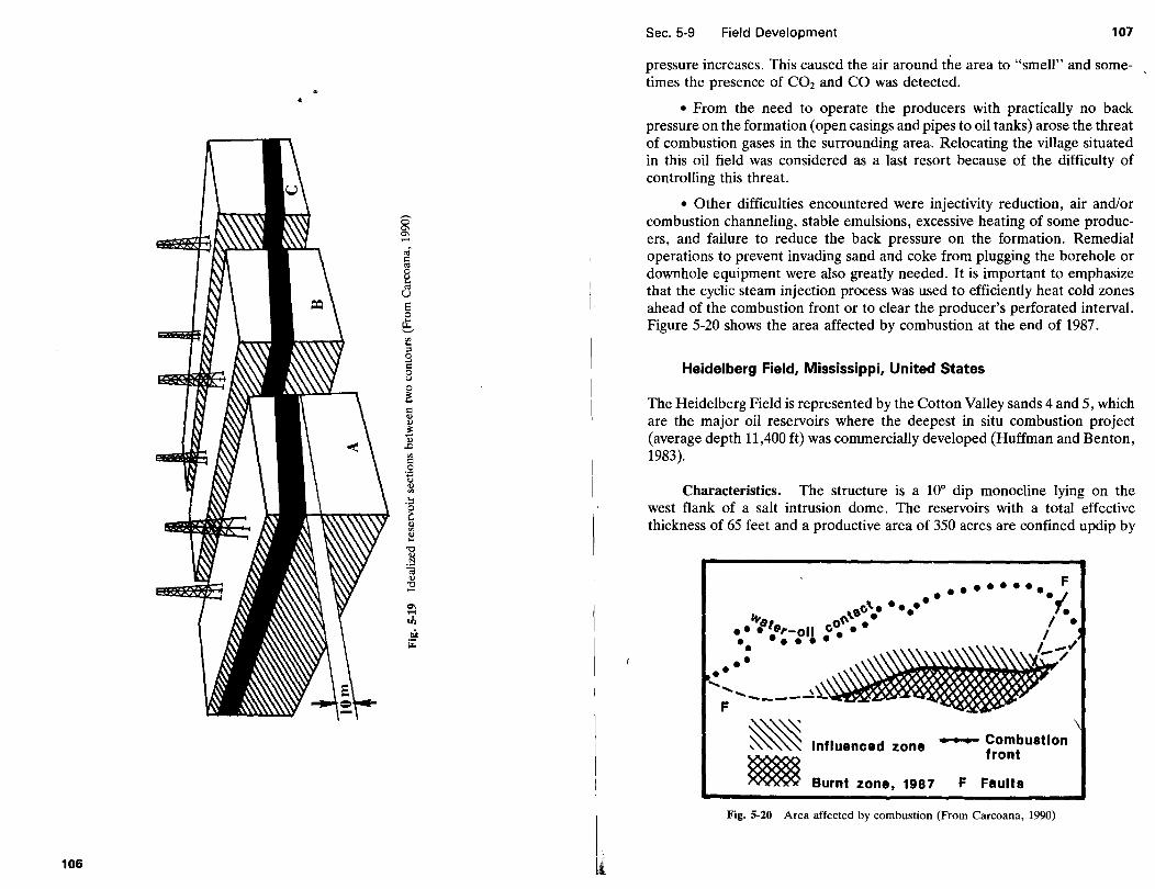
,-.._ 0 a, a, -~ c ~ 0 u .... ~ u E 0
~ "' .... ;::l
£ c 0 u 0
~ c Q) Q)
~ Q) ..c "' c
·~ Q)
"' -~ Q)
"' Q) .... "0 Q)
.!::l «< Q) "0 -~ .... o},
coil ~
106
I
I
Sec. 5-9 Field Development 107
pressure increases. This caused the air around the area to "smell" and sometimes the presence of C02 and CO was detected.
• From the need to operate the producers with practically no back pressure on the formation (open casings and pipes to oil tanks) arose the threat of combustion gases in the surrounding area. Relocating the village situated in this oil field was considered as a last resort because of the difficulty of controlling this threat.
• Other difficulties encountered were injectivity reduction, air and/or combustion channeling, stable emulsions, excessive heating of some producers, and failure to reduce the back pressure on the formation. Remedial operations to prevent invading sand and coke from plugging the borehole or downhole equipment were also greatly needed. It is important to emphasize that the cyclic steam injection process was used to efficiently heat cold zones ahead of the combustion front or to clear the producer's perforated interval. Figure 5-20 shows the area affected by combustion at the end of 1987.
Heidelberg Field, Mississippi, United States
The Heidelberg Field is represented by the Cotton Valley sands 4 and 5, which are the major oil reservoirs where the deepest in situ combustion project (average depth 11,400 ft) was commercially developed (Huffman and Benton, 1983).
Characteristics. The structure is a 10° dip monocline lying on the west flank of a salt intrusion dome. The reservoirs with a total effective thickness of 65 feet and a productive area of 350 acres are confined updip by
Influenced zone - Combustion front
Burnt zone, 1987 F Faults
Fig. 5-20 Area affected by combustion (From Carcoana, 1990)
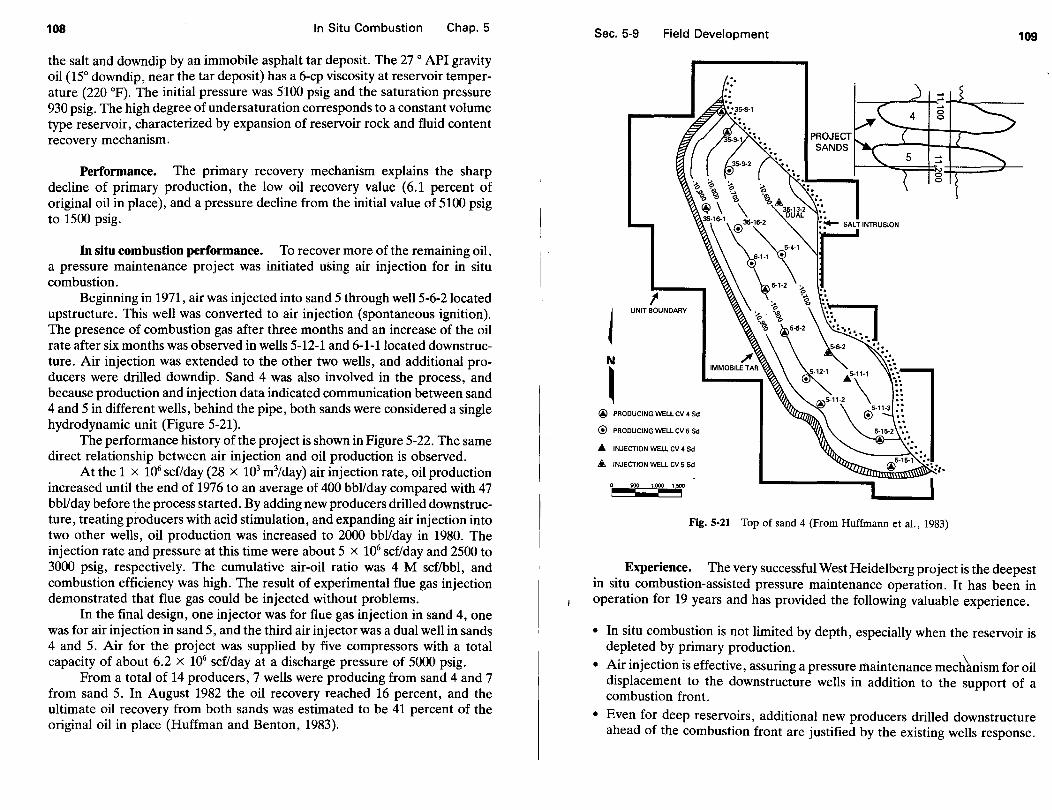
108 In Situ Combustion Chap. 5
the salt and downdip by an immobile asphalt tar deposit. The 27 o API gravity oil (15° downdip, near the tar deposit) has a 6-cp viscosity at reservoir temperature (220 °F). The initial pressure was 5100 psig and the saturation pressure 930 psig. The high degree of undersaturation corresponds to a constant volume type reservoir, characterized by expansion of reservoir rock and fluid content recovery mechanism.
Performance. The primary recovery mechanism explains the sharp decline of primary production, the low oil recovery value (6.1 percent of original oil in place), and a pressure decline from the initial value of 5100 psig to 1500 psig.
In situ combustion performance. To recover more of the remaining oil, a pressure maintenance project was initiated using air injection for in situ combustion.
Beginning in 1971, air was injected into sand 5 through well5-6-2located upstructure. This well was converted to air injection (spontaneous ignition). The presence of combustion gas after three months and an increase of the oil rate after six months was observed in wells 5-12-1 and 6-1-1located downstructure. Air injection was extended to the other two wells, and additional producers were drilled downdip. Sand 4 was also involved in the process, and because production and injection data indicated communication between sand 4 and 5 in different wells, behind the pipe, both sands were considered a single hydrodynamic unit (Figure 5-21).
The performance history of the project is shown in Figure 5-22. The same direct relationship between air injection and oil production is observed.
At the 1 x 10⁶ scf/day (28 x 103 m3/day) air injection rate, oil production increased until the end of 1976 to an average of 400 bbl/day compared with 47 bbl/day before the process started. By adding new producers drilled downstructure, treating producers with acid stimulation, and expanding air injection into two other wells, oil production was increased to 2000 bbl/day in 1980. The injection rate and pressure at this time were about 5 x 10⁶ scf/day and 2500 to 3000 psig, respectively. The cumulative air-oil ratio was 4 M scf/bbl, and combustion efficiency was high. The result of experimental flue gas injection demonstrated that flue gas could be injected without problems.
In the final design, one injector was for flue gas injection in sand 4, one was for air injection in sand 5, and the third air injector was a dual well in sands 4 and 5. Air for the project was supplied by five compressors with a total capacity of about 6.2 x 10⁶ scf/day at a discharge pressure of 5000 psig.
From a total of 14 producers, 7 wells were producing from sand 4 and 7 from sand 5. In August 1982 the oil recovery reached 16 percent, and the ultimate oil recovery from both sands was estimated to be 41 percent of the original oil in place (Huffman and Benton, 1983).
Sec. 5-9 Field Development
t UNIT BOUNDARY
@ PRODUCING WELL CV 4 Sd
<!) PRODUCING WELL CV 5 Sd
.A. INJECTION WELL CV 4 Sd
£ INJECTION WELL CV 5 Sd
500 1000 ,,
Fig. 5·21 Top of sand 4 (From Huffmann et al., 1983)
109
Experience. The very successful West Heidelberg project is the deepest in situ combustion-assisted pressure maintenance operation. It has been in operation for 19 years and has provided the following valuable experience.
• In situ combustion is not limited by depth, especially when the reservoir is depleted by primary production.
• Air injection is effective, assuring a pressure maintenance mech\nism for oil displacement to the downstructure wells in addition to the support of a combustion front.
• Even for deep reservoirs, additional new producers drilled downstructure ahead of the combustion front are justified by the existing wells response.
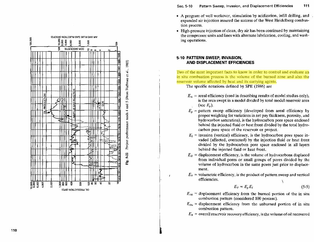
110
0 0 0
<"<
~ (B.LSHJSII\I) l:IOD ~ "' "' .,.
-~~= ····· . ..
N
~- ' ...
I!
I~ I~
-·· ::. I~ ... --- .-
0 0 0 0 00 0 0 qcoco ~
(OdB) NOI.LJnOOl:ld 110
... •:.--1~ t::: ~
···--1~ - ~
0 N
"'"'"' N
I~
' I
~
Sec. 5-10 Pattern Sweep, Invasion, and Displacement Efficiencies 111
• A program of well workover, stimulation by acidization, infill drilling, and expanded air injection assured the success of the West Heidelberg combustion process.
• High-pressure injection of clean, dry air has been continued by maintaining the compressor units and lines with alternate lubrication, cooling, and washing operations.
5-10 PATTERN SWEEP, INVASION, AND DISPLACEMENT EFFICIENCIES
Two of the most important facts to know in order to control and evaluate an in situ combustion process is the volume of the burned zone and also the reservoir volume affected by heat and its carrying agents.
The specific notations defined by SPE (1986) are
EA = areal efficiency (used in describing results of model studies only), is the area swept in a model divided by total model reservoir area (see Ep)·
EP = pattern sweep efficiency (developed from areal efficiency by proper weighting for variations in net pay thickness, porosity, and hydrocarbon saturation), is the hydrocarbon pore space enclosed behind the injected fluid or heat front divided by the total hydrocarbon pore space of the reservoir or project .
E1 = invasion (vertical) efficiency, is the hydrocarbon pore space invaded (affected, contacted) by the injection fluid or heat front divided by the hydrocarbon pore space enclosed in all layers behind the injected fluid or heat front.
En = displacement efficiency, is the volume of hydrocarbons displaced from individual pores or small groups of pores divided by the volume of hydrocarbon in the same pores just prior to displacement.
Ev =volumetric efficiency, is the product of pattern sweep and vertical efficiencies. \
(5-5)
Enb = displacement efficiency from the burned portion of the in situ combustion pattern (considered 100 percent).
Enu = displacement efficiency from the unburned portion of in situ combustion pattern.
ER = overall reservoir recovery efficiency, is the volume of oil recovered

112 In Situ Combustion Chap. 5
divided by the volume of hydrocarbon in place at the start of the project.
(5-6)
The scheme of a combustion front advancing in an oil reservoir is given in Figure 5-23 with an explicit presentation of the notions just defined (Burger and Carcoana, 1975).
The burned and unburned zones, the pattern sweep efficiency and the vertical efficiency appear clearly enough. It is important to note that pilot tests in the field and in commercial scale development of in situ combustion pointed to the existence of two unburned zones:
• Unburned zone I: inside the horizontal projection of the area covered by the combustion front; this zone was not observed in the lab experiments.
• Unburned zone II: strictly speaking, the zone in front of the combustion zone.
Injection Well
Corring Well
9
Production Well
10
Combustion Front
Fig. 5-23 Unburned zones, pattern sweep, and invasion efficiencies
Sec. 5-10 Pattern Sweep, Invasion, and Displacement Efficiencies
TABLE 5-1. Pattern Sweep Efficiency
Field
Delaware Childers, Oklahoma South Belridge, California S. Oklahoma, Oklahoma S.E. Kansas (Humbolt Chanute) Shannon, Wyoming Delhi, Louisiana Suplacu de Barcau, Romania Al3 Sloss, Nebraska Niitsu, Japan
Sweep Efficiencies
Pattern Sweep Efficiency, %
-100 -100
85 70 43 50 85 50
-100
113
The pattern sweep efficiency EP is determined approximately in the field by controlling the location of the combustion front at a given time. For an enclosed five-spot well pattern the flow of injected air and combustion gases relative to the movement of the oil corresponds to an infinite mobility ratio for choosing the areal sweep efficiency. Different modeling techniques show in this case an areal sweep efficiency of 62.6 percent, limited by practical considerations to 55 percent (Nelson and McNiel, 1961).
Some of the sweep efficiency values obtained in different five-spot pattern projects are presented in Table 5-1.
The higher values occurred because the inverted five-spot patterns were not confined.
The vertical sweep efficiency E1 is determined by taking postcombustion core samples. These indicate thickness of the burned zone and the amount of coke formed in the zone swept by the combustion front. It can also be determined taking into consideration the fact that the resistivity of the burned zone is 2 to 10 times higher than before combustion. The vertical sweep efficiency E1 is largely dependent on the thickness of the formation and has higher values for thinner pay zones.
The Delhi (Louisiana) project, where the thickness of the pay zone was only 2.5 ft, was characterized by a vertical sweep efficiency E1 value close to unity. In the North Tisdale project, core samples taken from a well drilled in the area swept by combustion showed vertical efficiency E1 = 27%. This time the burned portion of the formation thickness was located in the middle of the pay zone and not in the upper half as usual. Other E1 values reported ranged between 26 percent (South Oklahoma) to 50 percent (Trix Liz, Texas) and 60 percent (Emma Fry III, Illinois, and South Belridge, California), with an average value of 35 to 40 percent obtained at Suplacu de Barcau (Romania).

114 In Situ Combustion Chap. 5
It is important to note that the burned zone is a clean sand with improved porosity and permeability.
The displacement efficiency Evu for the unburned zone I is known by the oil saturation values taken from core samples. For instance, the North Tisdale project had a displacement efficiency Evu =50% of the initial oil content, and the South Belridge (California) oil saturation value within the unburned zone I was less than half of the initial oil content. In the Suplacu de Barcau project the bottom coring of three wells drilled in the area swept by the combustion front shows an average value of Evu = 43% (Turta, 1972, 1974).
The displacement efficiency Evu for the unburned zone II is very difficult to estimate. The oil from the unburned zone II is influenced by heat conduction. This increases its mobility and thereby makes it more easily displaced by the uncontrolled movement of the combustion front fluids. A bottom coring well drilled on a water-based mud in the unburned area II in the North Tisdale combustion project showed the following oil saturations (Martin and Alexander, 1971):
40% at the top of the production formation 32% in the median zone 50% at the bottom of the pay zone
compared with So = 60% at the start of the project. Assuming an average value of 40 percent, the displacement efficiency in zone II is Evu = 33%.
5-11 OIL CONSUMED IN SITU
As a result of distillation and thermal cracking, the oil consumed in situ deposits on the rock the coke available for combustion. The amount of oil (fuel) consumed is a function of the reservoir characteristics and of the volumetric sweep efficiency, Ev of the process. For instance, assuming reservoir rock porosity is 26 percent and oil saturation at the start of the project is 70 percent, the oil consumed for a fuel content Cu = from 0.8 to 2.6lbm/ft3 varies between 5.8 and 19 percent for Ev = 100% and between 1.7 and 5.7 percent for Ev = 30%.
Example 5-5. Calculate the oil consumed in an in situ combustion process developed on a reservoir with 23 percent porosity and 63 percent oil saturation. The fuel content is 1. 7 lbm/fe and the volumetric efficiency is 26 percent.
SOLUTION Oil in place (per unit volume)
N = V X <f> X So = 1 te X 0.23 X 0.63 = 0.1449 te
Sec. 5-11 Oil Consumed In Situ 115
Oil consumed per 1 fe of burned rock
Cu = 1.7Jbm
Given the specific gravity coke SG = 1.2, the volume of the oil consumed is
N' = Cu c SG X Pwater
(5-7) 1. 7 Ibm _ 3 3
1.2 x 62.5 lbmlfe - 0.0226 ft per 1 ft of burned rock
and the oil consumed as a percentage of the oil in place, when Ev = 0.26, is given by
(5-8) 0.0226
= 100 X 0
.1449
X 0.26 = 0.04 x (100) or 4% of the oil in place
The value of the parameter So'""' can also be known every moment by solving the ratio
S = cumulative air injected 0"'"' minimum air necessary oil in place at the start
X to burn 1 Ibm of fuel of the process
(5-9)
Example 5-6. Calculate the oil consumed after 5 years of in situ combustion developed as a primary recovery method. The oil reservoir (SG = 0.950) has 157 x 106 bbl OOIP reserve, and the combustion process is sustained by the injection of 700 x 103 te air/day through each of the 12 injection wells.
SOLUTION Cumulative air injected is
12 wells x 700 x 103 scf/day x 365 days x 5 yr = 15.33 x 10⁹ scf
Minimum air necessary to burn 1 pound of fuel is usually between 160 to 192 scf/lbm. Assuming a value of 186 scf/lbm and coke's specific gravity SG = 1.2, the minimum air necessary to burn 1 bbl of fuel is given by
186 scfllbm x SG x Pw lb/fe = 186 x 1.2 x 62.55 = 13,961 scf!fe
or
13,961 scf 5.614 bbl = 2487 scflbbl
For a value of 0.9 oxygen utilization, the oil consumed is
S = 15,330 X 106 scf X 0.90 _ 0"'"' 2487 scf/bbl X 157 X 106 bbls X
100 - 3·5% of OOIP
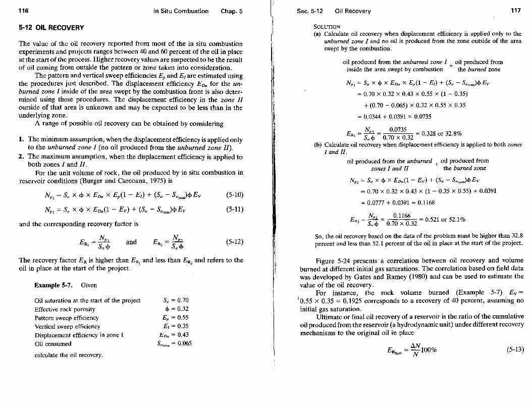
116 In Situ Combustion Chap.5
5-12 OIL RECOVERY
The value of the oil recovery reported from most of the in situ combustion experiments and projects ranges between 40 and 60 percent of the oil in place at the start of the process. Higher recovery values are suspected to be the result of oil coming from outside the pattern or zone taken into consideration.
The pattern and vertical sweep efficiencies Ep and E1 are estimated using the procedures just described. The displacement efficiency EDu for the unburned zone I inside of the area swept by the combustion front is also determined using these procedures. The displacement efficiency in the zone II outside of that area is unknown and may be expected to be less than in the underlying zone.
A range of possible oil recovery can be obtained by considering
1. The minimum assumption, when the displacement efficiency is applied only to the unburned zone I (no oil produced from the unburned zone II).
2. The maximum assumption, when the displacement efficiency is applied to both zones I and II.
For the unit volume of rock, the oil produced by in situ combustion in reservoir conditions (Burger and Carcoana, 1975) is
Np1
= So X <!> X EDu X Ep(1 - EJ) + (So - SoconJ<J> Ev
Np 2 = So X <!> X EDu(1 - Ev) + (So - SoconJ<J> Ev
and the corresponding recovery factor is
and
(5-10)
(5-11)
(5-12)
The recovery factor ER is higher than ER, and less than ER2 and refers to the oil in place at the start of the project.
Example 5-7. Given
Oil saturation at the start of the project Effective rock porosity Pattern sweep efficiency Vertical sweep efficiency Displacement efficiency in zone I Oil consumed
calculate the oil recovery.
So= 0.70
<I>= 0.32 Ep = 0.55 £ 1 = 0.35
EDu = 0.43
So000, = 0.065
Sec. 5-12 Oil Recovery 117
SOLUTION
(a) Calculate oil recovery when displacement efficiency is applied only to the unburned zone I and no oil is produced from the zone outside of the area swept by the combustion.
oil produced from the unburned zone I oil produced from inside the area swept by combustion + the burned zone
Np, = So X <f> X EDu X Ep{1 - £,) + (So - Sooo.,,)<f> Ev
= 0. 70 X 0.32 X 0.43 X 0.55 X (1 - 0.35)
+ (0. 70 - 0.065) X 0.32 X 0.55 X 0.35
= 0.0344 + 0.0391 = 0.0735
NPI 0.0735 ER, = So <I> = O. 70 X 0_32 = 0.328 or 32.8%
(b) Calculate oil recovery when displacement efficiency is applied to both zones I and II.
oil produced from the unburned + oil produced from zones I and II the burned zone
Np 2 =So X <J> X EDu(1 - Ev) +(So- So 00n,)<f>Ev
= 0.70 X 0.32 X 0.43 X (1 - 0.35 X 0.55) + 0.0391
= 0.0777 + 0.0391 = 0.1168
_ NP2 _ 0.1168 _ % ER2- So <I> -
0_70
X 032 - 0.521 or 52.1 o
So, the oil recovery based on the data of the problem must be higher than 32.8 percent and less than 52.1 percent of the oil in place at the start of the project.
Figure 5-24 presents a correlation between oil recovery and volume burned at different initial gas saturations. The correlation based on field data was developed by Gates and Ramey (1980) and can be used to estimate the value of the oil recovery.
For instance, the rock volume burned (Example 5-7) Ev = 10.55 x 0.35 = 0.1925 corresponds to a recovery of 40 percent, assuming no initial gas saturation.
Ultimate or final oil recovery of a reservoir is the ratio of the cumulative oil produced from the reservoir (a hydrodynamic unit) under different recovery mechanisms to the original oil in place
(5-13)
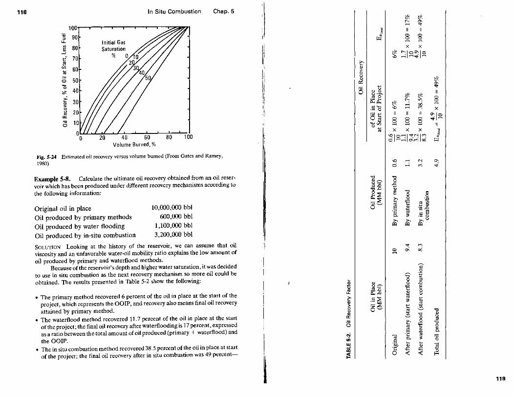
118 In Situ Combustion Chap.5 ~ ~ t-- 0\ ,..... '<:!"
100 ~ II a; 90 "" I ~~ 0 0
u... Initial Gas 0 0
"' 80
il ....... ,.....
"' X X
"' ...J
.... 70 % ~ 1'-:loO:Io ... \0 '!"""'' '!"""''~ '!""""'
"' .... ;>,
en 60 ...
.... <l.)
"' > 0
·- 50 u
0 <l.) ~ ~ 0\ -0
'#. 40 6 u ""'" <l.) <l.) II u ._,
~ ~ ~ 30
"' 0 0
"' - ... t-: IJ"l 0
> ~~ ~ oO ......
0
...... u
C'- \0 ...... ("') X Q)
-~ 0
a: == ..... II II O:lo
·-o; 0 0 0 '<:!",.....
0 .... 0 0 0
'0~ ...... ....... ...... X X X -;;;
60 80 100 ~~o.-;1"":~1"! .B "' o ,.....,..... 0\<'1 ao ~
Volume Burned,%
Fig. 5-24 Estimated oil recovery versus volume burned (From Gates and Ramey, 1980)
\0 ...... ('.1 0: 0 ,....; «)
""'" Example 5-8. Calculate the ultimate oil recovery obtained from an oil reser- '0 '0
voir which has been produced under different recovery mechanisms according to <ll,-..., 0 u- ..c ;::l.O .....
the following information: '0.0 <l.)
'0 8~ E c 0
·~ ::~ ;>, 0
Original oil in place 10,000,000 bbl ... 'E ;::l "' 6'-" "' .§ <l.)
.... ;::l ·~ .0
Oil produced by primary methods 600,000 bbl ~ ~ E ... !:!; 0.. -~ 0
;>, ;>, ;..,U
Oil produced by water flooding 1,100,000 bbl ~ ~ ~
Oil produced by in-situ combustion 3,200,000 bbl
SOLUTION Looking at the history of the reservoir, we can assume that oil '<:!" ("')
viscosity and an unfavorable water-oil mobility ratio explains the low amount of 0 o\ ao ......
oii produced by primary and waterflood methods. Because ofthe reservoir's depth and higher water saturation, it was decided
,-...., c
to use in situ combustion as the next recovery mechanism so more oil could be ,-...., .g obtained. The results presented in Table 5-2 show the following:
'0 "' 0 0 ;::l
8--- 0 .0 ti o:s- .;:::; E ~
_.o ... 0
• The primary method recovered 6 percent of the oil in place at the start of the ~.0
<l.) ..... u ~ .s~ "' .....
project, which represents the OOIP, and recovery also means final oil recovery !:!; ...
Q) :-;:::~ "'
attained by primary method. > ..... ..... 0 0'-" ... "' (.J .s '-" '0
• The waterflood method recovered 11.7 percent of the oil in place at the start Q) "' '0 <l.)
a: '-" 0 u ;::l
of the project; the final oil recovery after waterflooding is 17 percent, expressed 0 ;>, 0 '0 ... 'E "' 0
as a ratio between the total amount of oil produced (primary + waterflood) and i ·a <l.) l5..
l'li ~
the OOIP. .;, C<i 0.. !:!; ·a I
c • The in situ combustion method recovered 38.5 percent of the oil in place at start
w "5h ... ... C<i ..I
<l.) <l.)
m ·c 4:: 4:: .....
of the project; the final oil recovery after in situ combustion was 49 percent-
l j! 0 < < ~
119

120 In Situ Combustion Chap. 5
the ratio between the total amount of oil produced (primary + waterflood + in situ combustion) and the OOIP.
The amount of oil produced under one or more recovery mechanisms can also be referred to as the original oil in place.
In the example, the effect of waterflood increased the final oil recovery with 11 percent absolute value from 6 to 17 percent, and the effect of in situ combustion increased the final oil recovery with 32 percent absolute value (3.2/10 x 100 = 32%), from 17 to 49 percent.
The final (ultimate) oil recovery of a reservoir can only be improved by changing its recovery mechanism. Reaching the final oil recovery, within the limits of the same recovery mechanism, depends on the reservoir characteristics and operating conditions.
5-13 SCREENING CRITERIA
The dry or wet in situ combustion process has been used at a wide range of oil reservoirs to enhance oil recovery. It is possible to use a screening guide to assess the technical feasibility of the process on a specific oil reservoir (Carcoana, 1976; Chu, 1982; White, 1985).
Reservoir Characteristics
Depth and pressure
Temperature
Thickness Porosity Permeability (absolute)
Oil viscosity Reservoir oil saturation at start of project
Depth higher than 300 ft, the upper limit is conditioned by pressure which increases the cost of air compression. Air injection in shallow reservoirs should avoid reaching the parting pressure of the formation to prevent environmental pollution. Not critical. The higher the temperature, the better the chances for spontaneous ignition. Greater than 10ft. Higher than 16 to 18 percent. Higher than 100 md for viscous oils or shallow reservoirs with limited air injection pressures; higher than 30 md for less viscous oils and deeper formations. Less than 5000 cp (a moderate high viscosity). Higher than 25 to 30 percent. (In situ combustion may be applied after waterflooding.)
Sec. 5-14 Injection of Oxygen-Enriched Air or Pure Oxygen 121
Formation type Sands and sandstones; also carbonates with primary porosity.
Oil type With asphalt and naphtha compounds; also rocks with metals content, dirty sands.
In addition to these screening criteria, the recovery mechanism and the reservoir geometry must be considered to assure project success, whether or not other factors are favorable or adverse. Factors favoring the in situ combustion development include
• high values for cl> k, So, effective/gross thickness, and temperature. • low vertical permeability. • dependable well cementing job.
Adverse factors are
• high rock heterogeneity for gas and airflow. • Large gas-cap area. • emulsifying tendency of the produced oil, sanding, corrosion, and heat
damage to casing, cement, tubing, and pumps. • large thickness and low temperature of the horizontal productive forma
tions. • the decrease of the vertical efficiency by the gravity override to the upper
portion of the reservoir.
Research and more experience are needed to prevent and/or eliminate some of these adverse factors. ·
5-14 INJECTION OF OXYGEN-ENRICHED AIR OR PURE OXYGEN
i'he performance of in situ combustion can be improved by injecting, instead of air, oxygen-enriched air or pure oxygen. Moore received a U.S. patent on this method in 1965, but only recently has interest in its use increased and several companies now have lab experiments and projects in operation (Cady and Moss, 1981; White and Fairfield, 1982; Moore and Bennion, 1987; Petit, 1987).
Evident advantages of the use of oxygen instead of air are
• The decrease in the amount of gas to be compressed and injected because large volumes of nitr6gen are now eliminated. This increases the possibility
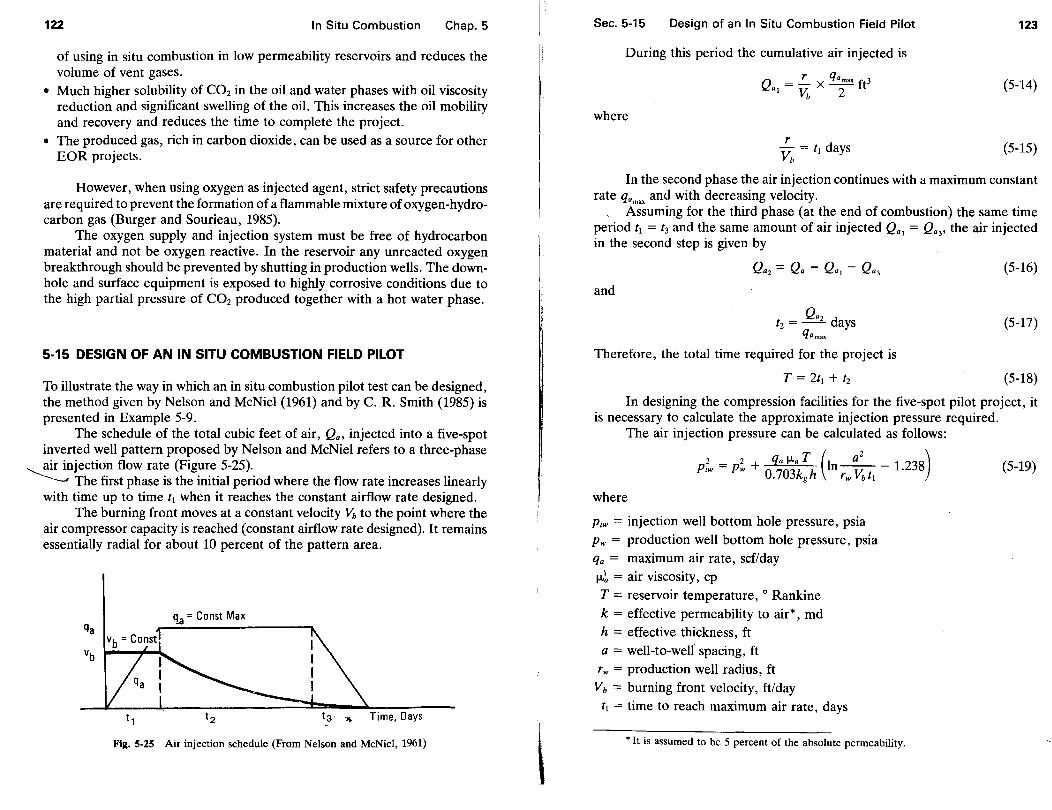
122 In Situ Combustion Chap. 5
of using in situ combustion in low permeability reservoirs and reduces the volume of vent gases.
• Much higher solubility of C02 in the oil and water phases with oil viscosity reduction and significant swelling of the oil. This increases the oil mobility and recovery and reduces the time to complete the project.
• The produced gas, rich in carbon dioxide, can be used as a source for other EOR projects.
However, when using oxygen as injected agent, strict safety precautions are required to prevent the formation of a flammable mixture of oxygen-hydrocarbon gas (Burger and Sourieau, 1985).
The oxygen supply and injection system must be free of hydrocarbon material and not be oxygen reactive. In the reservoir any unreacted oxygen breakthrough should be prevented by shutting in production wells. The downhole and surface equipment is exposed to highly corrosive conditions due to the high partial pressure of C02 produced together with a hot water phase.
5-15 DESIGN OF AN IN SITU COMBUSTION FIELD PILOT
To illustrate the way in which an in situ combustion pilot test can be designed, the method given by Nelson and McNiel (1961) and by C. R. Smith (1985) is presented in Example 5-9.
The schedule of the total cubic feet of air, Qa, injected into a five-spot inverted well pattern proposed by Nelson and McNiel refers to a three-phase air injection flow rate (Figure 5-25). ~ The first phase is the initial period where the flow rate increases linearly
with time up to time t1 when it reaches the constant airflow rate designed. The burning front moves at a constant velocity Vh to the point where the
air compressor capacity is reached (constant airflow rate designed). It remains essentially radial for about 10 percent of the pattern area.
'!a = Const Max
Time, Days
Fig. 5-25 Air injection schedule (From Nelson and McNiel, 1961)
Sec. 5-15 Design of an In Situ Combustion Field Pilot 123
During this period the cumulative air injected is
Q _ .!..._ qamax f 3
a!- Vb X 2 t (5-14)
where
r vb = t! days (5-15)
In the second phase the air injection continues with a maximum constant rate qam•x and with decreasing velocity.
Assuming for the third phase (at the end of combustion) the same time period t1 = t3 and the same amount of air injected Q.1 = Qa3, the air injected in the second step is given by
and
Qaz d t2 = -- ays qamax
Therefore, the total time required for the project is
T = 2t1 + t2
(5-16)
(5-17)
(5-18)
In designing the compression facilities for the five-spot pilot project, it is necessary to calculate the approximate injection pressure required.
The air injection pressure can be calculated as follows:
2 _ 2 qa !-La T (I a2
) P;w- Pw + 0.703kgh n,w Vbt
1- 1.238
where
Piw = injection well bottom hole pressure, psia Pw = production well bottom hole pressure, psia qa = maximum air rate, scf/day 1-L~ = air viscosity, cp T = reservoir temperature, o Rankine k = effective permeability to air*, md h = effective thickness, ft a = well-to-welf spacing, ft
r w = production well radius, ft vb = burning front velocity, ft/day
t1 =time to reach maximum air rate, days
*It is assumed to be 5 percent of the absolute permeability.
(5-19)
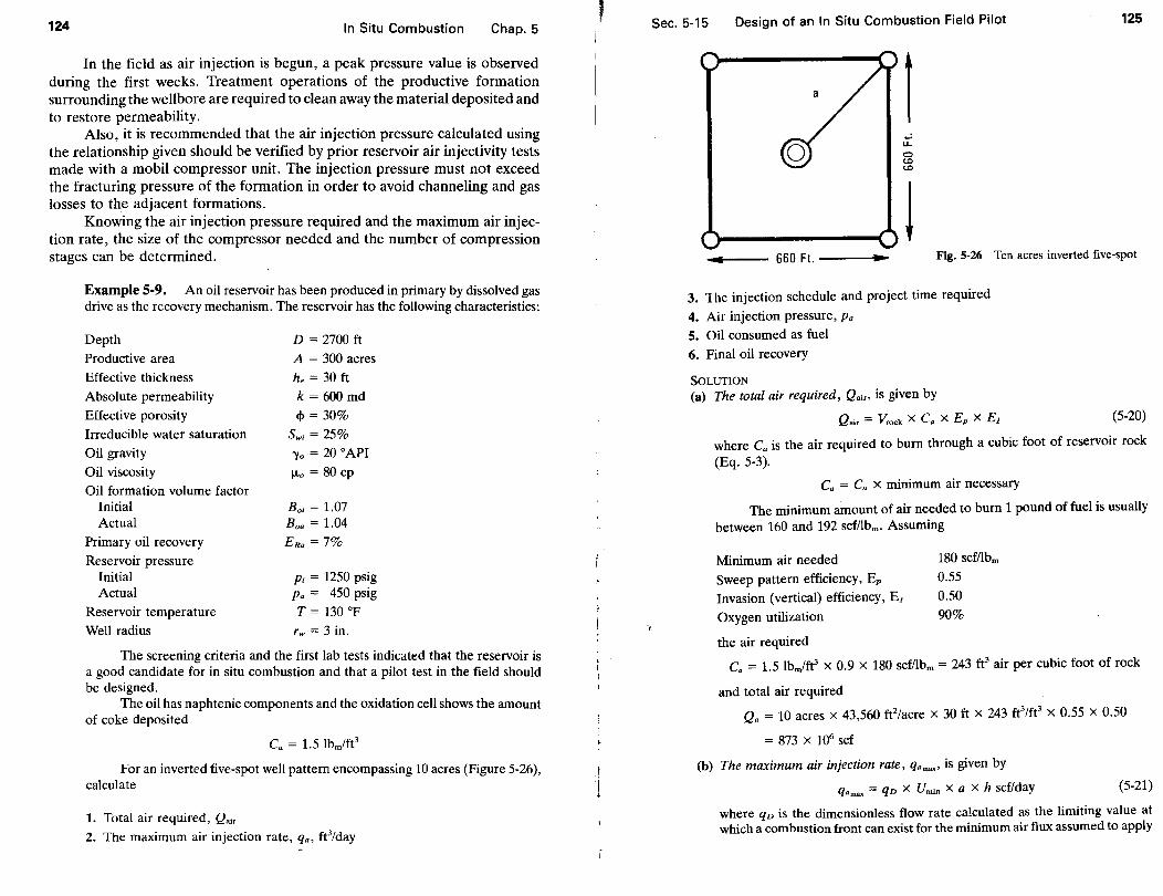
124 In Situ Combustion Chap. 5
In the field as air injection is begun, a peak pressure value is observed during the first weeks. Treatment operations of the productive formation surrounding the well bore are required to clean away the material deposited and to restore permeability.
Also, it is recommended that the air injection pressure calculated using the relationship given should be verified by prior reservoir air injectivity tests made with a mobil compressor unit. The injection pressure must not exceed the fracturing pressure of the formation in order to avoid channeling and gas losses to the adjacent formations.
Knowing the air injection pressure required and the maximum air injection rate, the size of the compressor needed and the number of compression stages can be determined.
Example 5-9. An oil reservoir has been produced in primary by dissolved gas drive as the recovery mechanism. The reservoir has the following characteristics:
Depth Productive area Effective thickness
Absolute permeability
Effective porosity Irreducible water saturation
Oil gravity Oil viscosity Oil formation volume factor
Initial Actual
Primary oil recovery
Reservoir pressure Initial Actual
Reservoir temperature Well radius
D = 2700 ft
A= 300 acres
he= 30ft k = 600 md
<!> = 30%
Swi = 25% 'Yo = 20 °API
f.Lo=80cp
Boi = 1.07 Boa = 1.04
ERa= 7%
P• = 1250 psig Pa = 450 psig T=l30°F
rw = 3 in.
The screening criteria and the first lab tests indicated that the reservoir is a good candidate for in situ combustion and that a pilot test in the field should be designed.
The oil has naphtenic components and the oxidation cell shows the amount of coke deposited
For an inverted five-spot well pattern encompassing 10 acres (Figure 5-26), calculate
1. Total air required, Qair
2. The maximum air injection rate, qa, fe/day
I' Sec. 5-15 Design of an In Situ Combustion Field Pilot 125
660Ft.---~
.... u.. 0 <0 <0
Fig. 5-26 Ten acres inverted five-spot
3. 1he injection schedule and project time required
4. Air injection pressure, Pa 5. Oil consumed as fuel
6. Final oil recovery
SOLUTION (a) The total air required, Qairo is given by
Qair = Yrock X Ca X Ep X E1 (5-20)
where Ca is the air required to burn through a cubic foot of reservoir rock (Eq. 5-3).
Ca = Cu X minimum air necessary
The minimum amount of air needed to burn 1 pound of fuel is usually between 160 and 192 scf/lbm. Assuming
Minimum air needed Sweep pattern efficiency, EP Invasion (vertical) efficiency, E1
Oxygen utilization
the air required
180 scfllbm
0.55
0.50 90%
Ca = 1.5 lbm/ft3 x 0.9 x 180 scfllbm = 243 ft3 air per cubic foot of rock
and total air required
Qa = 10 acres x 43,560 ff/acre x 30 ft x 243 ft3/fe x 0.55 x 0.50
= 873 x 106 scf
(b) The maximum air injection rate, qam•x' is given by
qamu = qv X Umin X a X h scf/day (5-21)
where qv is the dimensionless flow rate calculated as the limiting value at which a combustion front can exist for the minimum air flux assumed to apply
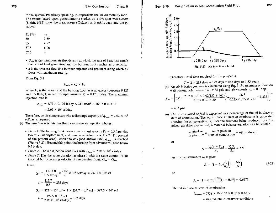
126 In Situ Combustion Chap.5
to the system. Practically speaking, q0 represents the air-oil mobility ratio. The results based upon potentiometric studies on a five-spot well system (Smith, 1985) show the areal sweep efficiency at breakthrough and the qv values.
Ep (%) qv 50 3.39 55 4.77
57.5 6.06
62.6 00
• Umin is the minimum air flux density at which the rate of heat loss equals the rate of heat generation and the burning front reaches zero velocity.
• a is the shortest flow line between injector and producer along which air flows with maximum rate, qa.
From Eq. 5-1
where Vb is the velocity of the burning front as it advances (between 0.125 and 0.5 ft/day); in our example assumes Vb = 0.125 ft/day. The maximum injection rate is
qam~ = 4.77 x 0.125 ft/day x 243 scf/fe x 466.7 ft x 30ft
= 2.02 x 10⁶ scf/day
Therefore, an air compressor with a discharge capacity of qam~ = 2.02 x 10⁶
scf/day is required. (c) The injection schedule has three successive air injection phases:
• Phase 1. The burning front moves at a constant velocity Vb = 0.5 ft per day (for efficient displacement) and remains radial until r = 117.7 ft (10 percent of the pattern area), when the designed airflow rate, qam•x' is reached (Figure 5-27). Beyond this point, the burning front advance will drop below 0.5 ft/day.
• Phase 2. The air injection continues with qamax = 2.02 X 10⁶ scf/day. • Phase 3. Has the same duration as phase 1 with the same amount of air
injected but decreasing velocity of the buming front, Qa, = Qa1•
Hence,
117.7ft 2.02 Qa 1 = 0_5 ft/day X - 2- X 106 scf/day = 237.7 X 10⁶ scf
117.7 t1 = ()."5 = 235 days
Qa 2 = 873 x 106 scf- 2 X 237.7 x 106 scf = 397.5 x 10⁶ scf
397.5 x 10⁶ scf fz = 2.02 x 10⁶ scf/day ~ 197 days
.. I
!.·
Sec. 5-15 Design of an In Situ Combustion Field Pilot 127
t 1 235 Days t2 358 Days t3 235 Days
Fig. 5-27 Air injection schedule
Therefore, total time required for the project is
T = 2 x 235 days + 197 days = 667 days or 1.83 ~ears . (d) The air injection pressure is calculated_ using E~. ~-19, _assum~g productiOn
well bottom hole pressure Pw = 35 psta (and au vtscos~ty fLa - 0.02 cp.)]112
2 2.02 X 106
X 0.02(130 + 460) In 660 _ 1.238 Piw = [35 + 0.703 X 30 X 30 0.125 X 235 X 3/12
= 607 psia
(e) The oil consumed as fuel is expressed as a percentage of t~e o~l in place at start of combustion. The oil in place at start of combustiOn ts calculat~d knowing the oil saturation, So. For the reservoir bein? produced b~ a dtssolved gas drive mechanism, a material balance equatiOn can be wntten.
original oil = oil in place at_ + oil produced in place, N start of combustiOn
or
and the oil saturation So is given
Bo ( t:J,.N) So = (1 - Swi) Boi 1 - N (5-22)
or
S = (1 - 0 25) l.04
(1 - 0.07) = 0.6779 0
• 1.07
The oil in place at start of combustion
Nae~ual = 7758 X 10 X 30 X 0.30 X 0.6779
= 473,354 bbl in reservoir conditions

128 In Situ Combustion
The percentage of oil consumed using Eq. 5-8 is
S 100 1.5 lbm/fe ocons = 1.2 X 62.5 lbm/fe
7758 bbVacres-ft(10 acres)(30 ft) X 473,354 bbl 0·55 X 0·50
= 2.70% of the oil in place at start of combustion
or the percentage of oil consumed using Eq. 5-9 is
Chap. 5
S = 873 X 106 scf X 100 . o=n• 180 scf/lbm X 1.2 X 62.5 lbm/ft3 X 473,354 bbl X 5.614 felbbl
= 2.43% of the oil in place at start of combustion
the amount of oil consumed is
473,354 bbl(2·~~o+x2243) = 12,141 bbl
and
12,141 bbl 7758 bbVacres-ft 10 acres x 30 ft x 0.3(1 - 0.25) = 0·023
or 2.3% of the original oil in place (0 Final oil recovery is the total oil produced, by a primary mechanism and by
combustion, from the original oil in place. Oil produced by combustion is given by Eqs. 5-10 and 5-11, assuming
the displacement efficiency EDu = 0.40.
Np 1 = 0.6779 X 0.30 X 0.40 X 0.55 X (1 - 0.5)
( 0.027 + 0.0243) + 0.6779 - 2 X 0.3 X 0.55 X 0.5 = 0.07618
NP2 = 0.6779 X 0.30 X 0.40(1 - 0.55 X 0.50) + 0.05381 = 0.11278
and the recovery factor by combustion ranges between
E _ 0.07618 _ RI - 0.6779 X 0.3 - 0·374 and 0.11278
ERz = 0.6779 X 0.3 = 0.554
and can be taken as (0.374 + 0.554)/2 = 0.464 or 46.4 percent of the oil in place at start of combustion.
The final oil recovery of the reservoir is
E = O 07 0.464(473,354) Rfinal • + 523 665
' = 0.4894 or 49% from the original oil in place
If a pilot successfully passes evaluation, plans are made to develop in situ combustion as a full-scale process. A number of five-spot well patterns have to be operated simultaneously and successively until the entire reservoir pro-
Chap. 5 Questions and Problems
I Air in'ection rate MS.C.F.D.
I I
I I
I
I I
I I
I I
I I I
I I
r- _T2~L .£~!! _ i!!i!cti,!!Q.. ra,!4!_ io.r .P!..Ole£.t~ I A4 84
I I
I I
A1 ~tern No
Fig. 5-28 Programming air injection, where a number of five-spot patterns are to be operated (From Nelson and McNiel, 1961)
129
ductive area is influenced by combustion. Nelson and McNiel provided a program for the simultaneous operation of a number of patterns (Figure 5-28).
To develop an in situ combustion process, the specific reservoir geometry and characteristics must be considered and a total air injection rate determined for the project such that a compressor's loading approaching 100 percent could be maintained.
For instance, in a five-spot well pattern development (Figure 5-28), pattern A 1 is first ignited. When this pattern reaches its maximum injection rate, pattern A 2 is ignited, and so on. The four patterns are fully operated after 4 x t1 days, and in this way the duration of the project is unnecessarily extended. The delay can be avoided if the four patterns are simultaneously ignited (in a two- to three-week period). As it was pointed out, each oil reservoir has its own geometry and characteristics. The reservoir engineer must
~ apply the most appropriate development program based on these characteristics to facilitate the flow of reservoir liquids to producers, to increase combustion efficiency, and to assure the most effective utilization of the compressors' capacity.
QUESTIONS AND PROBLEMS
5-l An oxidation cell experiment reveals two successive oxidation reactions. Which is the more important reaction and why?
5-2 How does the reactivity of different oils indicate whether or not they are good candidates for in situ combustion?

132 In Situ Combustion Chap. 5
ALDEA, G., V. PETCOVICI, et al., In Situ Combustion Field Test Pilot in Romania (original title: Aplicarea Experimentala a Metodei de Exploatare Prin Combustie Subterana in Romania), Petrol, Si Gaze, Vol. 19, No. 1, pp. 26-36 (1968).
BENHAM, A L., and F. H. POETTMANN, "The Thermal Recovery Process-An Analysis of Laboratory Combustion Data," Transactions of the A/ME, Vol. 213 (1958), pp. 83-85.
BURGER, J., A CARCOANA, eta!., "Basic Research on In-Situ Combustion and Recent Field Results," Paper no. PD-14-4 presented at the Ninth World Petroleum Congress, Tokyo, May 1975.
BURGER, J., and B. SAHUQUET, "Chemical Aspect of In-Situ Combustion, Heat of Combustion and Kinetics," Society of Petroleum Engineers Journal, Vol. 12 (1972), pp. 410-412.
BuRGER, J., and B. SAHUQUET, "Laboratory Research on Wet Combustion," Journal of Petroleum Technology, Vol. 25 {1973).
BURGER, J., P. SOURIEAU, eta!., Thermal Methods of Oil Recovery (Houston, TX: Gulf, 1985; Paris: Editions Technip), p. 284.
CADY, G. V., and J. T. Moss, "The Design and Installation of an Oxygen Supported Combustion Project in Lindbergh Field, Alberta, Canada," Paper presented at the 1981 World Oil and Gas Show, Dallas, Texas, December 14-17, 1981.
CARCOANA, A, "Results and Difficulties of the World's Largest In-Situ Combustion Process: Suplacu de Barcau Field, Romania," SPE/DOE paper 20248 presented at the SPE/DOE Seventh Symposium on Enhanced Oil Recovery, Tulsa, Oklahoma, April 22-25, 1990.
CARCOANA, A, and GH. ALDEA, Increasing Ultimate Oil Recovery (original title: Marirea Factorulni Final de Recuperare Ia Zacamintele de Hidrocarburi) (Bucarest, RO: Ed. Technica, 1976).
CARCOANA, A, V. C. MACHEDON, eta!., "In-Situ Combustion-An Effective Method to Enhance Oil Recovery in Romania," Special paper SP8, presented at the Eleventh World Petroleum Congress, London, 1983.
CHU, C., "A Study of Fireflood Field Projects," Journal of Petroleum Technology (February 1977).
CHU, C., "State-of-the-Art Review of Fireflood Field Projects," Journal of Petroleum Technology (January 1982).
COUNIHAN, T. M., "A Successful In-Situ Combustion Pilot in the Midway Sunset Field, California," Paper presented at the 1977 SPE California Regional Meeting, Bakersfield, California, April 13-15, 1977.
CRAWFORD, P. D., "Thermal Recovery Guide Helps Select Projects," World Oil {August 1, 1971).
FAROUQ ALI, S.M., "A Current Appraisal of In-Situ Combustion Field Test," Journal of Petroleum Technology (April 1972).
GADELLE, C. P., eta!., "Heavy Oil Recovery by In-Situ Combustion," SPE paper 8905 presented at SPE 50th California Regional Meeting, Los Angeles, California, April 9-11, 1980.
GADELLE, C. P., J. C. BURGER, eta!., "Heavy'Oi! Recovery by In-Situ CombustionTwo Field Cases in Romania," Journal of Petroleum Technology (November 1981).
Chap.5 References 133
GATES, C. F., and H. J. RAMEY, JR., "A Method for Engineering In-Situ Combustion Oil Recovery Projects," Journal of Petroleum Technology (February 1980).
GATES, C. F., and I. SKLAR, Combustion as a Primary Recovery Process-Midway Sunset Field, 1985 ed., SPE Reprint Series, No.7 "Thermal Recovery Processes" (Society of Petroleum Engineers, 1985), p. 359.
GRANT, B. F., and S. E. SAsz, "Development of an Underground Heat Wave for Oil Recovery," Transactions of the A/ME (1954).
HOWARD, F. A, "Method of Operating Oil Well," U.S. Patent #1,473,348 (XI-1923).
HUFFMAN, G. A, J. P. BENTON, et al., "Pressure Maintenance by In-Situ Combustion, West Heidelberg Unit, Jasper County, Mississippi," Journal of Petroleum Technology (October 1983).
JOSEPH, C., and W. H. PusH, "A Field Comparison of Wet and Dry Combustion," Journal of Petroleum Technology (September 1980).
KHUN, C. S., and R. L. KOCH, "In-Situ Combustion-Newest Method of Increasing Oil Recovery," Oil and Gas Journal (August 1953).
LATIL, M., Enhanced Oil Recovery (Houston, TX: Gulf, 1980). MACHEDON, V., eta!., "Evolution et Controle du Processus de Combustion Souter
raine," Proceedings, International Symposium on Hydrocarbons, Exploration, Drilling and Production Techniques, Paris, 1975.
MARTIN, W. L., J.D. ALEXANDER, eta!., "Thermal Recovery at North Tisdale Field, Wyoming," SPE paper no. 3595 (1971).
MOORE, R. G., D. W. BENNION, et a!., "New Insights into Enriched Air In-Situ Combustion," SPE paper 16740, 1987 SPE Annual Technical Conference and Exhibition, Dallas, Texas, September 27-30, 1987.
MooRE, T.V., U.S. Patent #3,208,519 (1965). NELSON, T. W., and J. S. McNIEL, "How to Engineer an In-Situ Combustion Project,"
Oil and Gas Journal (June 5, 1961). PARRISH, D. R., and F. F. CRAIG, JR., "Laboratory Study of a Combination of Forward
Combustion and Waterflooding-The COFCAW Process," Journal of Petroleum Technical (June 1969).
PARRISH, D. R., C. B. POLLOCK, and F. F. CRAIG, JR., "Evaluation of COFCAW as a Tertiary Recovery Method, Sloss Field, Nebraska," Journal of Petroleum Technology (June 1974).
PETCOVICI, V., "Considerations sur les Possibilites du Controle du Front de Combustion In Situ sur Champ," Revue de l' Institut Franf(ais du Petrole, Vol. 25 (1970), pp. 1355-1374.
PETIT, H. J. M., "In-Situ Combustion with Oxygen-Enriched Air," SPE paper 16741, 1987 SPE Annual Technical Conference and Exhibition, Dallas, Texas, September 27-30.
SMITH, CH. R., Mechanism of Secondary Oil Recovery (Malabar, FL: Robert E. Krieger, 1985), p. 406.
SPE Letter and Computer Symbols Standard (Richardson, TX: Society of Petroleum Engineers, 1986).
TRANTHAM, J. C., and J. W. MARX, "Bellamy Field Test Oil from Tar by Counteiflow Underground Burning," SPE of AIME Paper 1269 (October 1965).

134 In Situ Combustion Chap. 5
TuRTA, A., "Results of Continuous Bottom Coring of K3, Kt, and K2 Wells Drilled in the Pattern Area of the In-Situ Combustion Pilot in Suplacu de Barcau Oil Field," technical paper (Cimpina, RO: ICPPG, 1972, 1974).
TURTA, A., GH. ALDEA, and M. ZAMFIR, "The In Situ Combustion Industrial Exploitation of Suplacu de Barcau, Panonian Field, Romania," Paper presented at Fourth Unitar/UNDP International ConfereHce on Heavy Crude and Tar Sands, Edmonton, Canada, August 7-12, 1988.
VAN POOLLEN, H. C., and associates, Enhanced Oil Recovery (Tulsa, OK: Penn Well, 1980).
VOSSOUGHI, S., G. P. WILLHITE, eta!., "Automation of an In-Situ Combustion Tube and Study of the Effect of Clay on the In-Situ Combustion Process," Society of Petroleum Engineers Journal (August 1982).
WHITE, P. D., "In-Situ Combustion Appraisal and Status," Journal of Petroleum Technology (November 1985).
WHITE, p. D., and W. H. FAIRFIELD, "Oxygen Fire flood Is Source of Carbon Dioxide," Oil and Gas Journal (July 19, 1982).
WHITE, P. D., and J. T. Moss, Thermal Recovery Methods (Tulsa, OK: Penn Well, 1983), pp. 72-73.
WOLCOTT, E. R., "Method of Increasing the Yield of Oil Wells," U.S. Patent #1,457,479 (June 1923).
Chapter 6
Polymer Flooding
6-1 GENERAL
The waterflood field operations to increase the oil recovery, despite the successful development, resulted also in poor and incomplete sweeps of the reservoir volume. The first attempts to improve sweep efficiency in waterfloods were made by Detling (1944). He patented a number of additives, including
'water-soluble polymers, to increase the viscosity of injected water and the volume of the reservoir affected. In the next two decades over 25 patents for additives to be used under different reservoir conditions were issued and the first results of laboratory experiments dealing with their use were published (Sandiford l}nd Pye, 1964). Because of their lower cost, the water-soluble polymers prevailed over other additives (molasses, glycerin, glycols, etc.) tested in the field. After 1964, field test results and other significant laboratory studies (Mungan et al., 1966; Gogarty, 1967; Burcik, 1968; Maerker, 1972) made possible the development of polymer flooding as a method to enhance oil recovery.
135

136 Polymer Flooding Chap.6
6-2 PRINCIPLE AND METHOD DESCRIPTION
Water and Oil Mobilities
When water displaces oil through the reservoir's porous volume, the velocity of the displacement is proportional to the water mobility
kw Aw =-
J.Lw
where kw is the effective permeability of the rock to water in the water swept zone of the reservoir and J.Lw is the water viscosity. Water is the displacing phase and oil is the displaced phase. The oil also has a mobility
A = ko o J.Lo
where ko is the effective permeability of the rock to oil in the oil bank and J.Lo is the oil viscosity. Since the flow takes place under the same pressure gradient, the flow velocity is the same in the water swept area and in the oil bank zone only when Aw = Ao and the ratio A.wiA.o = 1.
Mobility Ratio Concept
The mobility ratio concept described by Craig (1980) is defined as the mobility of the displacing phase to the mobility of the displaced phase. In waterflooding,
M _ Aw = kw J.Lo w- 0 A
0 J.Lw ko
or, dividing by the absolute permeability, the water-oil mobility ratio
M = krwJ.Lo w-
0 J.Lwkro (6-1)
where k,w is the relative permeability to water at the average water saturation behind the waterfront and k,0 is the relative permeability to oil ahead of the flood front at irreducible water saturation.
It is obvious that when the mobility ratio is greater than unity, since J.Lw is less than J.Lo, water flows at a higher velocity through the path of least resistance and breaks through into producing wells prematurely. The mobility ratio in this case is deemed to be unfavorable.
Polymers Reduce Water-Oil Mobility Ratio
The role of water-soluble polymers is to increase the water viscosity and also to reduce the permeability of the rock to water, in other words, to reduce the
Sec. 6-2 Principle and Method Description 137
water-oil mobility ratio close to unity or less. Then, the volumetric sweep efficiency (areal x vertical) will be improved and a higher oil recovery will be achieved at breakthrough with polymer flooding than with waterflooding.
After water breakthrough into the producers, the flow of the two phases (water and oil) in the swept area of the reservoir is controlled by the fractional flow equation of Buckley and Leverett (1942),
t = 1 w 1 + (kofJ.Lo)(J.Lwfkw) (6-2)
where
fw = fraction of water in the flowing stream passing any point in the swept area (i.e., the water cut)
k 0 , kw = effective rock permeabilities to oil and to water, respectively, at one given water saturation at one point in the reservoir (Craig, 1980)
J.Lo, J.Lw = oil and water viscosities
Equation 6-2, simplified by ignoring the capillary pressure and gravitational effects, can also be expressed using relative rock's permeabilities to oil and water.
Again, it is easy to observe then when water viscosity J.Lw increases and the permeability of the rock to water kw decreases, the fractional flow of oil
t. =1-t =1-1
0
w 1 + (kro/J.Lo)(J.Lwfkrw) (6-3)
will increase, improving the rate of oil recovery. Permeability reduction and a higher water viscosity will increase the
resistance to flow of the polymer solution diverting it toward areas unswept by water.
Example 6-1. Given the water-oil relative permeability curves of an oil reservoir (Figure 6-1) and the ratio of viscosities J.Lolf..l.w = 6, calculate the water-oil mobility ratio Mw _ o and the water cut fw at Sw =50%.
SOLUTION Assuming the residual oil saturation in the waterflooded area of the reservoir, Sor = 0.20, and the irreducible water saturation in the oil bank ahead of the waterflood front, Sw, = 0.20, we read
k,w = 0.57 at So, and kro = 1.0 at Sw,
the water-oil mobility ratio
Mw-o = krw J.l.o = 0.57 X 6 = 3.4 f..l.w k,0 1.00
At Sw =50%
k,w = 0.13 and k,0 = 0.24

138 Polymer Flooding Chap.6
1.0------------------·
§ 0.9
-;,; CI:S 0.8 --~0.7 -:-:: 0 6 ...=· = ~ 5 0.5
""' ~ C..0.4 Q.l Ji> -0.3 CI:S --~ 0.2
0.1
o~--~1o~~2•o~~o~~4~o~~5~0--~6~o--~--~--~~1oo water saturation
Fig. 6-1 Water-oil relative permeability characteristics
the water cut
= 1 = 1 = 0.76 /w 1 + (k,)!J.o)(!J.wfk,w) 1 + (0.24 X 1)/6 X 0.13)
Method Description
In polymer flooding, a slug of 0.3 or higher PV of polymer solution is injected into the reservoir with a prior injection of a low-salinity brine (freshwater) slug. The polymer slug is followed by another freshwater slug and by continuous drive water injection. The schematic cross-section view of a polymer injection is given in Figure 6-2. "'
The polymer solution slug is injected between two freshwater buffers in order to attenuate the direct contact with the saline reservoir water. The saline water reduces the polymer solution's viscosity.
Many studies of the characteristics of polymers as water mobility control agents have been reported. A state-of-the-art review on polymer flooding
= 0 .... -..2 ""' 0 ! <IJ
CI:S ""' $ ~
-= 5 <IJ ~
.... ~ Q 0 ..:: c..
BEJBG
""'
.. :_ ·n· ·: .. . ··B· . : .......
. ~\· . . . . .. . . . . . . . . . . . . . . . . . . . . ·... :. . . . . I
. ' · ... · . : ,· I ." I I .. • I 1 .. 1 II
1111'·~··11 • . I· 1. · ,1 IN I' •I , . I . II I I
I I I
. . .
I. . I I • . . I ' I .. I· I .
'. • . · • I · I . I 1 I 1 I , I ·.· .. _,,··.:··.,····a · · .'·r. I .1. N • · · · · I' I I . . . . . I I' .. I
0 . . . . . . . .. ... ~ . . . . . . ~ o----'--~H-+-t+-1-+. +~-+-t-+-+·-+-·...J ~ . .... = ....
139

140 Polymer Flooding Chap. 6
and on the application of polymers for mobility control is given by Needham and Doe (1987) and Gao (1987), respectively.
Knowing the principle and method description it is now understood that polymer flooding does not reduce the residual oil saturation. It improves oil recovery over waterflooding by increasing the reservoir volume contacted. Also, in comparison to waterflooding, polymer flooding accelerates oil pr~du~tion, and a higher recovery is obtained at breakthrough. Polymer floodmg Is successful when applied in the early stages of a waterflood process or when applied at the beginning when the mobile o~l saturat~o? is high. !t ha~ litt~e or no effect in uniform waterflooded reservOirs contammg low-viscosity oil or having high water saturation at the start of the process. Reservoirs with high permeability variations, rapid water breakthrough i?to the produc~rs, and lo~ recoveries can also be flooded with polymer solutwns, but the nsk factor IS higher.
6-3 POLYMER TYPES
There are two principal types of polymers being used in field applications: hydrolyzed polyacrylamide (HP AM) and polysaccharides biopolymer or xanthan gum.
Polyacrylamides
The polyacrylamide is obtained by the polymerization of the acrylamide monomer. Through hydrolysis some of the acrylamide monomers are converted to carboxylate groups with a negative charge. The hydrolyzed polyacrylamide has a 20 to 40 percent degree of hydrolisis, a molecular weight higher than 3 x 10⁶ and a linear chain molecular structure. The long molecular chain of the partially hydrolyzed polyacrylamide, in solution with freshwater, eases the flow through the tortuous porous space of the rock reservoir. In saline water, the electrolytes in solution cause the molecules to coil. This obstructs the flow through the porous space and reduces the viscosity of the solution. The hydrolyzed polyacrylamide solution is sensitive to salts and must be prepared with freshwater. Other susceptibilities of H'PAM solutions are caused by the presence of oxygen, which is a source of instability and chemical degradation, and by temperature and mechanical degradation. The HPAM molecules' long chains may be broken, especially at high velocity and temperature conditions, when the injected solution passes through the well's perforated interval and flows through the porous space of the formation near the wellbore.
Being less expensive and providing higher residual resistance to drive
Sec. 6-4 Apparent Viscosity and Resistance Factor 141
water injection, polyacrylamide is more widely used in the field than polysaccharide as a water mobility control agent. However, recent tests have shown that microbial attack of polyacrylamide can be a potentially serious problem (Grula and Sewell, 1982) and biocides, such as formaldehyde, need to be used to prevent the viscosity loss caused by microbes.
Polysaccharides
The polysaccharide biopolymer is obtained from sugar in a fermentation process caused by the bacterium Xanthomonas campestris. The polysaccharide's molecular structure gives the molecules a great stiffness (Needham and Doe, 1987), their behavior being like rigid-rod molecules (Gao, 1987). As a consequence, in contrast to polyacrylamide polymer, the viscosity of a polysaccharide biopolymer solution is not affected by salinity, and shearing effects can be tolerated. Despite these advantages, the polysaccharide biopolymer is expensive, and its stability degrades at temperatures above 200 oF. Biodegradation by enzymes of polysaccharide polymers is also common and usually results in a decrease in the solution's viscosity. Formaldehyde is the most effective biocide added to biopolymers to prevent biodegradation.
6-4 APPARENT VISCOSITY AND RESISTANCE FACTOR
Apparent Viscosity
Polymers are used in aqueous solutions at low concentrations of 300 to less than 2000 parts per million (ppm) or 0.03 to less than 0.20 percent. The viscosity values of polymer solutions measured with an Ostwald viscometer, for different ~oncentrations, are plotted practically as a straight line on a semilog paper. The measured viscosity of the low-concentration polymer solutions used in the field is only 1 to 1.5 cp. It is interesting to observe that the behavior in a porous medium of these low-concentration polymer solutions suggests a much higher viscosity. Indeed, the viscosity of the polymer solution flowing in the reservoir is from 5 to 25 times higher when calculated indirectly using Darcy's equation (apparent viscosity), assuming the same effective permeability (Figure 6-3).
In reality, the effective permeability of the formation to a polymer solution is lower than it is to water without polymer. It is difficult to separate the effect of the permeability reduction from that of the viscosity increase. As we pointed out, what is important is that the total effect can be expressed as mobility reduction and this total effect can be measured.

142
100
60
40
20 0. <.J
·~ 0
-~ 10 > 6
4
2
1 0
~-r-~--
2 3 4
Polymer Flooding Chap.6
Fig. 6-3 Resistance effect of polymer 5 solution in porous media (From Pye,
Polymer concentration% 1964)
Resistance Factor
The measure of the mobility reduction is known as the resistance factor, R
where
R = Aw = k,wf~w = k,w ~p = Mw-o Ap krp/~p ~wkrp Mp-o
(6-4)
Ae = water-soluble polymer mobility k,w, kre = relative permeabilities to water and to polymer solution,
respectively ~e = viscosity of the polymer solution (apparent)
Mw _ 0 , Me_ o = water-oil and polymer solution-oil mobility ratios, respectively
A plot of the resistance factor R as function of the ratio V;n/Vp (cumulative injected volume per porous volume) is given in Figure 6-4.
The data were obtained by flowing a 300-ppm polymer solution through the porous volume of a core sample. A rapid' increase of the resistance factor from 1 to 8 was observed for the first 20 pore volumes injected. Continuing the polymer solution injection, the value of the resistance factor remained practically constant. This tendency of the resistance factor to stabilize must be observed in the laboratory tests for R values less than 10 or 12 to avoid in the field high injection pressures or blockages.
As a matter of fact, polymers with high resistance factors can be used in profile improvement to plug the more permeable streaks near injectors and to
Sec. 6-5 Polymer Retention
16
14
12
R 10
8
6
4
2
.
0 (0 201
T i
401 60 Vinj Vpor
!
!
80
"' "'
. 100 120
Fig. 6-4 The resistance factor "R" function of cumulative volume injected
143
reduce the variation in permeability. Also, polymers gelled with crosslinkers can be used in an effort to plug reservoir high-permeability zones far from injectors.
The advantages of polymers as water mobility control agents in porous mediums are indicated by the large resistance factor values obtained using water-containing low-polymer concentrations and by their ability to stabilize flow resistance.
Residual Resistance Factor
The measure of the reduction of rock's permeability to water after polymer flow ~s known as the residual resistance factor, RR.
RR = (k,wl~w) before polymer flow (k,wl~w) after polymer flow
(6-5)
Permeability reduction is observed after flushing with brine, following injection of a polymer solution, a Berea sandstone core sample. The original permeability of the core, having been reduced by adsorption on the rock surface and by mechanical entrapment of polymer molecules, cannot be recovered.
The existence of residual resistance effects has economic importance. Expenditures for polymer occur only during the injection period. Long afterward, the residual resistance factor effect continues at no added expense.
Biopolymer polysaccharides are not retained on rock surfaces. This is the reason they do not exhibit the residual resistance effect.
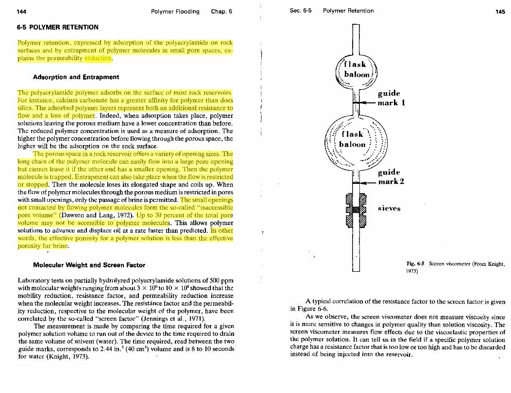
144 Polymer Flooding Chap.6
6-5 POLYMER RETENTION
Polymer retention, expressed by adsorption of the polyacrylamide on rock surfaces and by entrapment of polymer molecules in small pore spaces, explains the permeability reduction.
Adsorption and Entrapment
The polyacrylamide polymer adsorbs on the surface of most rock reservoirs. For instance, calcium carbonate has a greater affinity for polymer than does silica. The adsorbed polymer layers represent both an additional resistance to flow and a loss of polymer. Indeed, when adsorption takes place, polymer solutions leaving the porous medium have a lower concentration than before. The reduced polymer concentration is used as a measure of adsorption. The higher the polymer concentration before flowing through the porous space, the higher will be the adsorption on the rock surface.
The porous space in a rock reservoir offers a variety of opening sizes. The long chain of the polymer molecule can easily flow into a large pore opening but cannot leave it if the other end has a smaller opening. Then the polymer molecule is trapped. Entrapment can also take place when the flow is restricted or stopped. Then the molecule loses its elongated shape and coils up. When the flow of polymer molecules through the porous medium is restricted in pores with small openings, only the passage of brine is permitted. The small openings not contacted by flowing polymer molecules form the so-called "inaccessible pore volume" (Dawson and Lang, 1972). Up to 30 percent of the total pore volume may not be accessible to polymer molecules. This allows polymer solutions to advance and displace oil at a rate faster than predicted. In other words, the effective porosity for a polymer solution is less than the effective porosity for brine.
Molecular Weight and Screen Factor
Laboratory tests on partially hydrolyzed polyacrylamide solutions of 500 ppm with molecular weights ranging from about 3 x 10⁶ to 10 x 106 showed that the mobility reduction, resistance factor, and permeability reduction increase when the molecular weight increases. The resistance factor and the permeability reduction, respective to the molecular weight of the polymer, have been correlated by the so-called "screen factor" (Jennings et al., 1971).
The measurement is made by comparing the time required for a given polymer solution volume to run out of the device to the time required to drain the same volume of solvent (water). The time required, read between the two guide marks, corresponds to 2.44 in. 3 (40 cm3
) volume and is 8 to 10 seconds for water (Knight, 1973).
Sec. 6-5 Polymer Retention
guide ~---mark2
sieves
145
Fig. 6-5 Screen viscometer (From Knight, 1973)
A typical correlation of the resistance factor to the screen factor is given in Figure 6-6.
As we observe, the screen viscometer does not measure viscosity since it is more sensitive to changes in polymer quality than solution viscosity. The screen viscometer measures flow effects due to the viscoelastic properties of the polymer solution. It can tell us in the field if a specific polymer solution charge has a resistance factor that is too low or too high and has to be discarded instead of being injected into the reservoir.

146
~
e u
"' u..
"' u <::
~ ·;:;; Q)
a:
Polymer Flooding
30~----------------------~------.
20
10
Berea Sandstone k = 250 m D
HPAM 500 ppm Solution with 3% NaCI + 0.3% CcCI 2
I
0+-------~-------.--------~------~ 0 10 20 30 40
Screen Factor
Chap.6
Fig. 6-6 Typical correlation of the resistance factor with the screen factor (From Jennings et al., 1971)
6-6 FIELD PROJECTS AND RESULTS
After the first field experiments and project evaluations made by Jewett and Schurz in 1970, the application of water-soluble polymers to field projects has increased. Currently polymer flooding is being used on a commercial scale as a method of recovering more oil.
Field Projects
Comprehensive surveys of the published results of full-scale polymer flood case histories have been conducted by Manning et al. (1983) and by Needham and Doe (1987), among others. An adapted statistical analysis of the fieldwide polymer flood projects is shown in Table 6-1.
The fieldwide projects were performed principally in sandstone reservoirs. The carbonate lithologies made a relatively small contribution to polymer flooding. The pay zones were characterized by depths between 400 ft and 11 000 ft with a 4000 ft average, by 117 op mean temperature with 229 op m~imu~ value, and by a good average porosity of 19 percent. The rock permeabilities ranged from the very low value of 1.5 md to a maximum of740? md with 453 md the mean value. The permeability variation (Lorenz coefficient) ranged from 0.07 (practically a uniform reservoir) to 0.96 (for a highly heterogeneous reservoir) with the mean value being 0.69. The viscosities ofthe reservoir crude oils where polymer flooding was applied ranged from very low
Sec. 6-6 Field Projects and Results 147
TABLE 6-1. Polymer Flood Statistics
Fieldwide Projects
Number of Standard Parameter Projects Min Max Mean Deviation
Depth, ft 87 400 10,800 4005 2201 Temperature, op 88 46 229 117 34 Porosity 87 0.19 Average permeability, md 80 1.5 7,400 453 1107 Permeability variation 71 0,07 0.96 0.69 0.19 Oil viscosity, cp 82 0.072(?) 435 21.45 51.48 Water-oil ratio at start 42 0 75 5.3 11.77 Average polymer
concentration, ppm 48 51 600 279 149 Water-to-oil
mobility ratio 49 0.1 40 7.86 9.71 Oil recovery,% OOIP 20 0 14 3.85 3.62 Oil recovery, STB/acre-ft 23 0 143.4 34.4 40.07 Oil recovery, STB/lb 18 0 11.20 3.74 3.50
From Manning et al. (1983).
values to a maximum 435 cp with an average value of 21.4 cp. The water-to-oil mobility ratio ranged from 0.1 to 40, the mean value being 7.86. The water-oil ratio at start of the polymer flood had values corresponding to water-free oil production rates (WOR = 0) up to a maximum of WOR = 75 (water cut 98.6 percent) in postwaterflood applications.
The polymer used in the majority of these applications was polyacrylamide, and only a few projects utilized polysaccharide biopolymer.
Field Results
The maximum oil recovery was 14 percent of the original oil in place (OOIP). The mean value was close to 4 percent of OOIP in 20 fieldwide projects. In any case, the recovery was greater than with waterflooding alone. In 23 fieldwide projects, the maximum recovery was 143 STB/acre-ft, and the mean recovery value was 34.4 STB/acre-ft.
The injection of high-molecular-weight, water-soluble polymer has become a recognized enhanced oil recovery (EOR) method. In the United States, EOR production from polymer flooding has increased in the last decade. It still represents only approximately 4 percent of total EOR production, with thermal methods comprising approximately 80 percent. There are now wellestablished guidelines for successfully applying polymer flooding and for obtaining maximum recovery and additional oil (Chang, 1978; Gao, 1987; Needham and Doe, 1987).

148 Polymer Flooding Chap. 6
6-7 GUIDELINES FOR POLYMER APPLICATION
Reservoir Characteristics
Reservoir depth is a critical factor only when related to reserv?ir temperature. Temperatures less than 200 oF as~ure. a .stable ?olym~r ~ol~t10n.
Reservoir pressure is not critical If It permits the mJe~hon pre~sure t~ be less than the formation parting pressure and is not so high that It reqmres
expensive pumping equipment. . . . The porosity of the reservoir rock must be medmm to high (higher than
18 percent) to assure a good storage capac~ty. . . Absolute permeability of the reservmr rock IS considered to be good
between 50 and to 250 md. Moderate permeability values (between 15 and 50 md) cause higher injection pressures. Permeability values considered very good (between 250 and 1000 md) and excellent (higher than 1000 md) assure higher recoveries with conventional waterflood and leave polymer flood ex-penses difficult to justify. . .
The permeability variation concept connected With reservOir heterogene-ity is better than permeability alone. for determining. areas of polymer flood applicability. Heterogeneous reservmrs are g?od candidates for p~lymer floo?ing for two reasons. First, the polymer solutio~ reduces the rocks permeabi~ity. Second, the solution has a tendency to ~tvert towa~d unswept reservou areas or areas where waterflooding resulted m an unsatisfactory sweep.
Fluid Characteristics
The oil viscosity that directly controls the water-oil mobility ratio should not be higher than 150 to 200 cp. Viscosity of less than 100 cp is even more preferable. Thermal methods of recovery are competitive when reservoirs' oil viscosities are high. When they are low, less than 5 cp, waterflood and/or other EOR methods may be preferred.
The water-oil ratio at the start of the project should be low, even zero. This will mean higher mobile oil saturation. Polymer flooding applied from the beginning as a secondary recovery process instead of waterflooding will afford better chances of success than waterflooding.
Reservoir Selection
As stated, polymer flooding is successfully applied as a secondary recovery process when the mobile oil saturation in res~rvoir is still ~i~h. '!'he effect. of polymer flooding is to improve areal and vertical sweep effic~encies, reducmg the water-oil mobility ratio and diverting the injected fluid toward larger reservoir areas. Polymer flooding does not improve the displacement effi-
Sec. 6-7 Guidelines for Polymer Application 149
ciency, since it has no effect on the existing capillary forces and interfacial tensions.
Waterflooded oil reservoirs can also be good candidates for polymer flooding. This is only true, however, when the high WOR values are caused either by a high water-oil mobility ratio (viscous oil reservoirs) and waterconning or by a low vertical sweep efficiency (heterogeneous reservoirs). Under these conditions, the reservoirs still have high mobile oil saturation which can be reduced by the diverting effect of polymer flooding and by the increase of vertical sweep efficiency. Therefore, the use of polymer as a tertiary method (after waterflooding) is attractive only if the high WOR is due to waterconning, high permeability zones or high oil viscosity. Large gas-cap areas and extensive aquifers should be avoided.
Incremental Oil Recovery
There are several methods to estimate initially the incremental oil recovery from polymer flooding. Johnson's (1956) simplified graphical treatment of the Dykstra-Parsons waterflood calculation method, the fractional flow predictive method of Patton and coworkers (1971), and the empirical correlations published in U.S. DOE Report DOE/ET 12072-2 (1987), among others, can be applied as a screening guide for polymer flood potential.
The technique is to compare the oil recovery expected through using <;ontinued waterflooding with the oil recovery expected using the modified flow properties from polymer flood.
Because of its simplicity, Johnson's graphical treatment of the Dykstra-Parsons method is still used throughout the oil industry when a rapid appraisal of a waterfloeld project is needed.
The technique is based upon the correlation for four variables, namely,
V = permeability variation Swi = initial water saturation M = water-oil mobility ratio ER = fractional recovery of oil in place, at a specified water-oil ratio, WOR
Figures 6-7, 6-8, 6-9, and 6-10 show plots correlating, V, M, Sw, and ER for WOR of 1, 5, 25, and 100, respectively.
The permeability variation, V (Craig, 1980) measures the effect of permeability stratification on flood-out performance. Since rock permeabilities usually have a log-normal distribution, the percentages of the total number of permeability values arranged in descending order are plotted on log probability graph paper (Figure 6-11), and a straight line is drawn through the points. The permeability variation is given by
V = k-:._ ka k
(6-6)
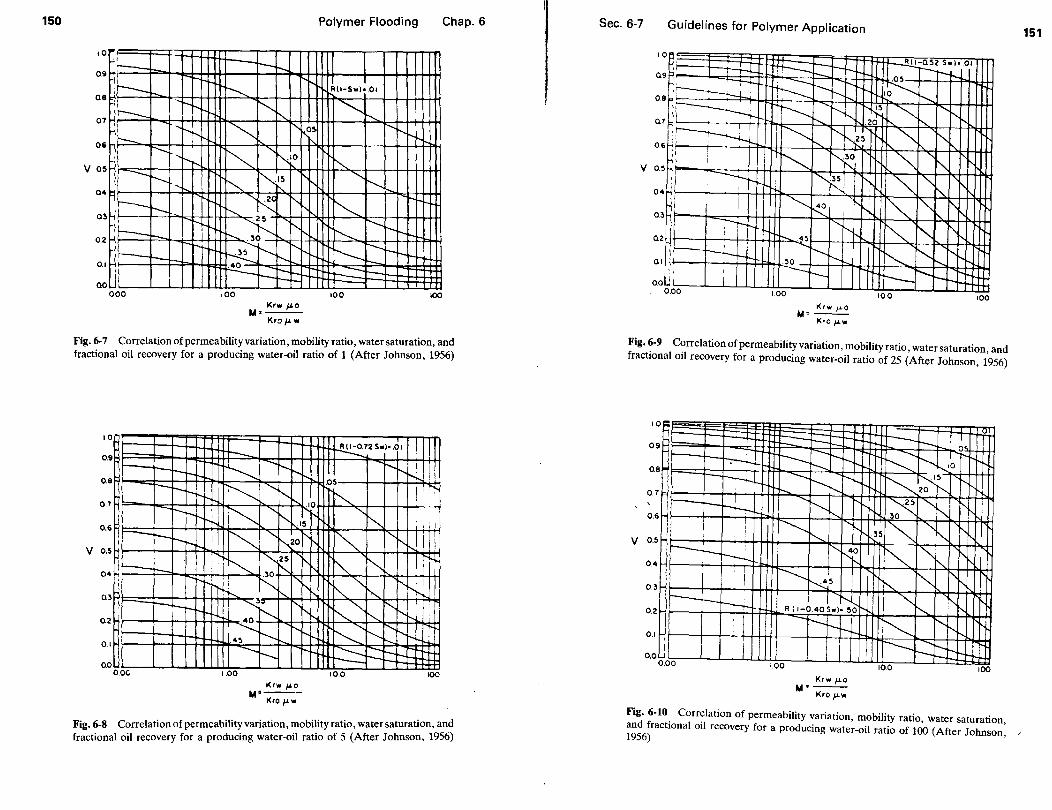
150
1.0
~· ~I:--
:~ lk_
0.9
0.8
0.7
0.6 i--
v 0.~ ---0.4
:---a 3
0.2 r---r--
0. I
ao 0.00
·-.. K I -......
!'-..
:----. ......
t---
Polymer Flooding Chap. 6
t-- t-. .I t--__
II r R(I·Swl• 01
I'-f'.... ""-..
........
~ 1'- r-,o~ f'.t---
""' ' "'10 ~
""' ~~~ "" '-......,
r-.... "~ t'--..._ ~ ~ ............
r-..... .30 '~ r---...... -~---......... I' 1--r-- 1-r-. ~~ !"--- ,_
~t- t- ~---- f.-1---1'- 1-
1.00 100 100 Krw }J-0
M•---KroiJ-w
Fig. 6-7 Correlation of permeability variation, mobility ratio, water saturation, and fractional oil recovery for a producing water-oil ratio of 1 (After Johnson, 1956)
1.0
0.9
--0.8
---~---0.1
--~---0.6 ~
h -1--t-.
H (I-
t;
v 0.~
0.4
(
0 3 ! ~
0.2
0. I
0. 0 o.oc
t+-~
..... !'--"r--
~ ......... r'-- t-... .10
~ ' "' .I~
" ~ f'.-20 "~' r . ~ ""'-2~ "r-• i .30 ['-.,
h-'1--... "'-r-- " ............. 3J
I"" !'---~ 1'-rl-4~ t---r--- rt
1.00
Krw }J-0 u=--Kro ~'-'"
~72Sw)•.OI 'l m t---. t--.t-1_1 1
! .0~
~ ! I I
"~ .. -
~ '~'- t-...1 i ~ "' IT
, I
~"" ""' I'. I)-I
:
t--......""' f'..._ i'f'. !
~'-..........' r----. "'~"--......
~ ~ t-r--100 100
Fig. 6-8 Correlation of permeability variation, mobility ratio, water saturation, and fractional oil recovery for a producing water-oil ratio of 5 (After Johnson, 1956)
Sec. 6-7 Guidelines for Polymer Application
a
os 9 p i----l. ,._,__
f-. I --:---<--0 ,r--~
8~
0. 7wc----=4 ~.~'
06 H H\ 5h, :/
v 0.
04 ~~ I
0.3
az \~
a I 1
ui 0.0 0.00
i --:.....:
I I
~ -.:._1-
I
I
tt+--=== 1--r-. ~-a 52 Swl• 01 1-- r--r-t--
K ~ "' ~ 1----- 10 r--.....
rr--~ t'-....r--- :.? ~ !'>. 'f'.
.20 "' -........... ~5 ""' I'-"" '""' ~ ""' ~
J ~ I' ~ "' ....... --............ ~T ~ "' 1\ I I ........
t"- r-._
'r---I ~ ' '" !-... .45
........ 1--- ......._ r--
.50 ~ !'---.. ['-... ---t--- r--- r---.. t-1.00 100 100
Fig. 6-9 Correlation of permeability variation, mobility ratio, water saturation, and fractional oil recovery for a producing water-oil ratio of 25 (After Johnson, 1956)
0.
ON
9 1- --0. 8
r.--r---
0. 7
~~' __;_ -
l
i!---.r--
H !---
I
0.6
v 0.5
0.4
0.3
~ 1--t--' 0.2
0. I
0.0 I
0.0 0
t-- - I-+-- +-
r-- --t--t-....
,......
............ r--....... r--. ~
'r--..... r-...... -..........
~ ~ K4o
[----.. ~5
1.00
1 ....... R ( 1-0.40 Sw)•.50 -t-t- ,......
Krw }J-0 u·--Kro ~'-"'
DT --t--I
.05
~ 1'-- I t"-~0
~ f'-<5 """ .20 !"'-.
~ ""' I'--30
35~ "' " ['..
~ ~ ....... ~
""" 1\
I ~ ' !'-...
~ r----1'-r----. t---1"'---~'--1-t--.
10.0 100
Fig. 6-10 Correlation of permeability variation, mobility ratio water saturation and fractional oil recovery for a producing water-oil ratio of u)o (After Johnson' 1956) '
151

152
where
..c "' Q)
§ Q)
0.. Q)
c. E "' en
Polymer Flooding
100,-----------------------------~
80 60
40 k-k11 10-3
V=---= --=0.7 k 10
20
k 10 ···················-·-·-··--
' 8 I I
6 : 4 k 11 : 3 ---------------------1-------
1 I I I I I
2 : I I I I I I I I I I I
.. '~ ' '
1 2 5 10 203040 607080 90 95 989999.5 Portion of Total Sample Having Higher Permeability
Fig. 6-11 Log. normal permeability distribution (From Craig, 1980)
Chap.6
k = mean permeability (the permeability value with 50 percent probability) k" = permeability at 84.1 percent of the cumulative sample
The values range from zero to one, a uniform reservoir having the permeability variation of zero.
For a calculated value of the permeability distribution V and a water-oil mobility ratio Mw _ 0 , the expression ER(1 - c x Sw) can be read at the intersection point on the plot for a producing WOR of 1 (Figure 6-6). The same procedure applied for WORs of 5, 25, and 100 makes it possible to know the variation of the fractional recovery of oil in place, ER for different producing WORs characterizing a conventional waterflood. The modified flow property of polymer flood is the water-oil mobility ratio reduced by the numerical value of the resistance factor R. Using this new mobility ratio, the fractional recovery of oil in place, ER, can be obtained for different producing WORs character'izing a continuous polymer flood. The difference in recovered oil for a given WOR value represents the incremental amount of oil due to the polymer project. The method assumes linear flow with pistonlike displacement and with no additional oil being produced after the passage of the front. As was pointed out, the method is a screening device which compares two types of flood under the same flowing conditions and is considered to give good relative answers.
Sec. 6-7 Guidelines for Polymer Application 153
TABLE 6·2. Properties of Example Reservoir
Irreducible water saturation Relative permeability for water Relative permeability for oil Water viscosity Oil viscosity Permeability variation Formation volume factor for oil Resistance factor
0.20 0.18 (at Sor) 0.60 0.473 cp 6.4 cp 0.5 1.05 6
Example 6-2. Compare, at a water cut of 95 percent, the final oil recovery ~actors expected _through conventional water injection and polymer waterfloodmg. The reservmr properties are shown on Table 6-2.
SOLUTION
(a) Mobility ratios:
Water-oil mobility ratio:
Resistance factor:
Mw _ 0
= krw j.Lo = 0.18(6.4) = 4 1-Lw kro 0.473(0.6)
R = krw j.Lp = 6 1-Lw krp
Polymer sol~tion-oil mobility ratio:
Mp - o = M~- o = 0.666
(b), Oil_re_covery fac~ors (Table 6-3): The WOR plotted against recovery factor ER ts Illustrated m Figure 6-12 for waterflood and for polymer flood. When the water cut, [w = 0.95, the water-oil ratio is
WOR = _.b..__ = 19 1- [w
and the recovery factor is ER = 33.0% for waterflood and ER = 41.6% for polymer flood.
TABLE 6-3. Oil Recovery Factors
M Oil Recovery WOR= 1 WOR=5 WOR = 25 WOR = 100 4 £R(1 - C X Swi) 0.11 0.205 0.32 0.38 ER,% 13.75 23.95 35.7 41.3 0.666 ER(l - C X Sw;) 0.20 0.30 0.38 0.425 ER,% 25 35 42.4 46.6

154
a: 0 10 5::
Polymer Flooding Chap.6
10 20 30 40 50 60
Fig. 6-12 Water-oil ratio versus oil recovery
Although the method assumes 100 percent volumetric sweep efficiency and continuous polymer solution injection, it still can be said that the additional oil recovery with polymer injection corresponds to an increase of 8 to 9 percent of OOIP over that obtained by waterflood. The oil reservoir can be selected as a polymer flood candidate.
6-8 DESIGN CONSIDERATIONS
After the reservoir selection is made, de_tailed testing is performed on the different polymers available for viscosity,. molecular weight, shear degradation, and adsorption. Different polymers' resistance factors are measured using representative core samples. Simulation studies are necessary to determine the optimum polymer concentration, the slug size, and the estimated oil recovery. Field injectivity tests are very useful to determine the polymer's behavior in the porous space of the reservoir and to design the appropriate polymer injection facilities and quality control. . . .
The reservoir engineer should take into account all the extstlng expen-ence regarding polymer flooding. Thorough consideration should be given to the specific reservoir characteristics and performances before the start of the
process. . .. To illustrate in some detail the work performed after an od reservotr ts
identified as a polymer flood candidate, a typical case history is presented.
Sec. 6-8 Design Considerations 155
Sleepy Hollow Reagan Unit, Nebraska, United States
The Reagan reservoir case history (Christopher et al., 1988) shows that the selection of the reservoir as a polymer flood candidate was made due to the unfavorable mobility ratio under waterflooding (the oil viscosity was 24 cp and injection water viscosity was 0.71 cp).
Laboratory tests were performed first to determine the viscosity, screen factor, and shear degradation characteristics of different polymer samples using the low salinity injection water. After choosing the polyacrylamide p~lymer, which provided the best results, porous media displacement tests usmg polymer solutions and residual saturation of a refined oil were performed to determine the measurement of the resistance factor and the residual resistance factor. The incremental oil recovery of 10.1 percent of OOIP from polymer flooding was estimated using the fractional flow predictive method (Patton et al., 1971 ). The 22-cp viscosity of the polymer solution flowing through the porous medium (the apparent viscosity) displaces to the right the fractional flow curve (Figure 6-13 ).
The value of the producing water cut was reduced as the polymer solution was diverted toward unswept or poorly swept areas of the reservoir. Using computer simulation techniques, the reservoir characteristics were described by history matching the waterflood performance on a three-dimensional black
c:: 0
- ·.;::; u e u. ~
~
0.8
~ 0.6 -0
~ 0
u.
"' c:: 0 ·~
~ 0.2 u.
Fractional Flow Curves
Legend •Water, 0.72cp D Poly., 22cp ---
0.8 Sw(Saturation of Displacing Fluid, Fraction)
Fig. 6-13 Fraction flow curves for water and 22-cp polymer solution displacing Reagan crude oil (From Christopher et al., 1988)
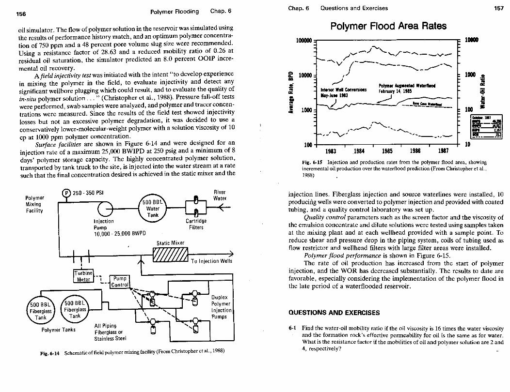
156 Polymer Flooding Chap.6
oil simulator. The flow of polymer solution in the reservoir was simulated using the results of performance history match, and an optimum polymer concentration of 750 ppm and a 48 percent pore volume slug size were recommended. Using a resistance factor of 28.63 and a reduced mobility ratio of 0.26 at residual oil saturation, the simulator predicted an 8.0 percent OOIP incremental oil recovery.
Afield injectivity test was initiated with the intent "to develop experience in mixing the polymer in the field, to evaluate injectivity and detect any significant wellbore plugging which could result, and to evaluate the quality of in-situ polymer solution ... " (Christopher et al., 1988). Pressure fall-off tests were performed, swab samples were analyzed, and polymer and tracer concentrations were measured. Since the results of the field test showed injectivity losses but not an excessive polymer degradation, it was decided to use a conservatively lower-molecular-weight polymer with a solution viscosity of 10 cp at 1000 ppm polymer concentration.
Surface facilities are shown in Figure 6-14 and were designed for an injection rate of a maximum 25,000 BWIPD at 250 psig and a minimum of 8 days' polymer storage capacity. The highly concentrated polymer solution, transported by tank truck to the site, is injected into the water stream at a rate such that the final concentration desired is achieved in the static mixer and the
Polymer Mixing Facility
Injection Pump 10,000 · 25,000 BWPD
All Piping Fiberglass or Stainless Steel
Duplex Polymer Injection Pumps
Fig. 6-14 Schematic of field polymer mixing facility (From Christopher et al., 1988)
Chap. 6 Questions and Exercises 157
Q Ct.. CD
~ 1111:
& I! .!
Polymer Flood Area Rates 100000 1-
........ -.J '- /-/i...,.. ""' --__,....,._
~v ;---.. ----.........- ....,..-- .............
10000 I 1000 t ,.../ Polymer Auplellted Waterftood 1111:
Interior Wtll ConYirsions flbrvary 14. 1915 ~ May-JuH 1913 _.-) ... ) ---~~-"!!'.!!! ___ !
1000 100 ~
100 +---..,.---...---...---.,------1- 10 1983 .1984 1985 1986 1987
Fig. 6-15 Injection and production rates from the polymer flood area, showing incremental oil production over the waterflood prediction (From Christopher et a!., 1988)
injection lines. Fiberglass injection and source waterlines were installed 10 producing wells were converted to polymer injection and provided with co~ted tubing, and a quality control laboratory was set up.
Quality control parameters such as the screen factor and the viscosity of the emul~i~n concentrate and dilute solutions were tested using samples taken at the mlXlng plant and at each wellhead provided with a sample point. To reduce shear and pressure drop in the piping system, coils of tubing used as flow restrictor and wellhead filters with large filter areas were installed.
Polymer flood performance is shown in Figure 6-15. . . !he rate of oil production has increased from the start of polymer mJectwn, and the WOR has decreased substantially. The results to date are favorable, e.specially considering the implementation of the polymer flood in the late penod of a waterflooded reservoir.
QUESTIONS AND EXERCISES
6-1 Find the water-oil mobility ratio if the oil viscosity is 16 times the water viscosity and the formation rock's effective permeability for oil is the same as for water. What is the resistance factor if the mobilities of oil and polymer solution are 2 and 4, respectively?
158 Polymer Flooding Chap. 6
6-2 A polymer injection test is conducted on a five-spot pilot with 10 acres (40,000 m2
) area, 20ft (6.1 m) effective thickness, and 25 percent porosity. A total amount of 0.28 PV of 350-ppm polymer solution has to be injected at a daily rate of 377 bbl (60m3
). Since the polyacrylamide is available in both as liquid and powder, calculate how long the test will take and what amount of liquid or powder HP AM should be mixed with water on site. The liquid has 8 wt % active polymer concentration and the powder has 95 wt % concentration.
6-3 Using the water-oil ratio versus oil recovery, percentage of OOIP (Figure 6-12), calculate the recoveries at breakthrough whenfw = 50% and after breakthrough when fw = 98% for both waterflood and polymer flood.
6-4 Compare, as a first screening, the oil recovery expected at breakthrough with conventional water injection and with polymer flooding. The reservoir has a permeability variation of V = 0.5, the oil-water viscosity ratio !Lofi.Lw = 5, the resistance factor R = 4, and the water-oil relative permeability characteristics are given in Figure 6-1.
6-5 How much additional oil, percent of OOIP, is produced by continuing the waterflood and the polymer flood up to water cut fw = 0.97?
6-6 Make comments regarding the recovery obtained at breakthrough and at a water cut of 97 percent with both water and polymer flood. Is the continuous polymer flood economically justified?
REFERENCES
BUCKLEY, S. E., and M. C. LEVERETT, "Mechanism of Fluid Displacements in Sands," Transactions of the A/ME, Vol. 146 (1942), pp. 107-16.
BuRCIK, J.E., "What, Why and How of Polymers for Waterflooding," Petroleum Engineering (August 1968). . .
CHANG, H. L., "Polymer Flooding Technology-Yesterday, Today and Tomorrow," Journal of Petroleum Technology (August 1978).
CHRISTOPHER, C. A., T. J. CLARK, and D. H. GIBSON, "Performance and Operation of a Successful Polymer Flood in the Sleepy Hollow Reagan Unit," Society of Petroleum Engineers/U.S. Department of Energy paper SPE/DOE 17395, SPE/DOE Sixth Symposium on Enhanced Oil Recovery, Tulsa, Oklahoma, April 17-20, 1988.
CRAIG, F. F., The Reservoir Engineering Aspects of Waterflooding, third printing (Richardson, TX: Society of Petroleum Engineers, 1980), pp. 45-46.
DAWSON, R., and R. LANTZ, "Inaccessible Pore Volume in Polymer Flooding," SPE Journal (October 1972).
DETLING, K. D., "Process of Recovering Oil from Oil Sands," U.S. Patent #2-341-500 (February 1, 1944 ).
GAO, HONG WEN, Mobility Control in Oil Recovery by Chemical Flooding, State-of-theArt Review, Topical Report NIPER-146 (DE87001210) (Bartlesville, OK: National Institute for Petroleum and Energy Research-U.S. Department of Energy, January 1987).
I'
Chap. 6 References 159
GOGARTY, W. B., "Mobility Control with Polymer Solutions," Journal of Petroleum Technology (June 1967).
GRULA, M. M., and G. W. SEWELL, "Microbial Interactions with Polyacrylamide Polymers," Proceedings, International Conference Microbial Enhancement Oil Recovery, E. C. Donaldson and C. J. Bennett, eds., Bartlesville, Oklahoma (1982), p. 219.
JENNINGS, R. R., J. H. ROGERS, and T. J. WEST, "Factors Influencing Mobility Control by Polymer Solutions," Journal of Petroleum Technology (March 1971).
JEWETT, R. L., and G. F. SCHURZ, "Polymer Flooding-A Current Appraisal," Journal of Petroleum Technology (June 1970).
JOHNSON, C. E., JR., "Prediction of Oil Recovery by Water Flood--A Simplified Graphical Treatment of Dykstra-Parsons Method," Transactions of the A/ME, Vol. 207 (1956), pp. 345-46.
KNIGHT, BRUCE L., "Reservoir Stability of Polymer Solutions," Journal of Petroleum Technology (May 1973).
MAERKER, J. M., "Dependence of Polymer Reaction on Flow Rate," Journal of Petroleum Technology (November 1972).
MAERKER, J. M., "Mechanical Degradation of Partially Hydrolyzed Polyacrylamide Solutions," SPE Journal (August 1976).
MANNING, R. K., G. A. POPE, L. W. LAKE, et al., A Technical Survey of Polymer Flooding,Projects, U.S. Department of Energy, Report No. DOE/BC/10327-19, September 1983.
MUNGAN, N., F. W. SMITH, and J. L. THOMSON, "Some Aspects of Polymer Floods," Journal of Petroleum Technology (September 1966).
NEEDHAM, R. B., and P. H. DoE. "Polymer Flooding Review," Journal of Petroleum Technology (December 1987), p. 1504.
PATTON, J. T., K. H. COATS, and G. T. COLEGROVE, "Prediction of Polymer Flood Performance," SPE Journal (March 1971), pp. 72-84.
PYE,DAVIDJ., "Improved Secondary Recovery by Control of Water Mobility," Journal of Petroleum Technology (August 1964), pp. 911-916.
SANDIFORD, B. B., "Laboratories and Field Studies of Water Floods Using Polymer Solution to Increase Oil Recoveries," Journal of Petroleum Technology (August 1964), pp. 917-22.
U.S. DEPARTMENT OF ENERGY, Economics of Enhanced Oil Recovery, Report DOE/ ET/12072-2 (Washington, D.C.: U.S. Department of Energy, 1981), pp. 19-20.
Chapter 7
Alkaline Flooding
7-1 GENERAL
Alkaline or caustic flooding is another method by which oil displacement efficiency can be improved. The benefits of this process have been known for a long time and were first observed by Squires (1917) and later by others. However, not until1942 did Subkow offer the explanation that alkaline agents such as sodium hydroxide could react with naturally occurring organic acids in crude oil to produce soaps at the water-oil interface. The effect produced in a reservoir appears to be similar to that of micellar solutions. The difference is that alkaline flooding reduces the interfacial tensions (IFf) with surfactants generated in situ.
Despite the fact that alkaline agents are less expensive, the benefits expected from alkaline flood have not been confirmed by firm field results and still remain a possibility rather than a reality. Indeed, the major difficulty is that the process appears to be highly dependent on minerals on the surface of reservoir rock, which are not chemically inert, and on the crude oil and injection fluid characteristics.
Efforts have been made, especially in the last decade, to understand
160 lj
Sec. 7-2 Displacement Mechanisms and Method Description 161
better the recovery mechanisms generated in alkaline flooding. Since alkaline agents are cost-efficient materials, their use, along with surfactant and/or polymer, could reduce the amount of high-cost surfactant and cosurfactant required in micellar flooding. A reevaluation of alkaline flooding is taking place in order to find ways to reduce the reaction of alkaline agents with reservoir minerals and to take advantage of the combined alkaline/surfactant mixture effect.
7-2 DISPLACEMENT MECHANISMS AND METHOD DESCRIPTION
Displacement Mechanisms
~everal mechanisms have been suggested regarding oil displacement by alkaline flooding. The publication of Johnson's review (1976) gives a description of four different mechanisms based on oil emulsification and wettability reversal. ,
It is known that fluid distribution within the pore spaces of a rock reservoir during (alkaline) waterflood depends upon the wetting and non wetting phase saturation and upon the direction of the saturation change (Craig, 1980). In a water-wet rock reservoir, the injected water increases the wetting phase saturation, the residual oil being the discontinuous phase. In an oil-wet rock reservoir, the injected water decreases the wetting phase saturation theresidual oil being the continuous phase. It was observed also that 'residual oil saturation always depends on the dimensionless ratio of viscous to capillary force.s def~ned as the capillary number: V~J-/cnj>: (velocity x viscosity of the dtsplacmg water) + (interfacial tension between water and oil phases x porosity). When the capillary number value can be increased from w-6
(conventional waterflood) to w-4 or more, the residual oil saturation decreases.
1. The alkaline solutions increase the capillary number value by reacting with the organic acids present in some crude oil to form emulsifying soaps. The petroleum soap or surfactant formed emulsifies oil and water and reduces the interfacial tension by two or three orders of magnitude. This mechanism is referred to as emulsification and entrainment because the oil-in-water emulsion formed is entrained by the fluid flow and can then be produced. The residual oil saturation is lowered and an incremental increase in oil recovery can result.
2. When the displacement takes place in an oil-wet reservoir where residual oil is a continuous p~~se,. the alkaline agent changes the inj~ction water piJ and the rock wettabthty 1s reversed from oil-wet to water-wet. This mech-

162 Alkaline Flooding Chap. 7
anism is defined as wettability reversal. As a consequence the water-oil relative permeability and the water-oil mobility ratio are lowered, with evident benefits on oil recovery (Mungan, 1966).
3. Even in the water-wet reservoirs the discontinuous, nonwetting residual oil phase can be changed to a continuous wetting phase if proper conditions of reservoir temperature, pH, and salinity of the alkaline solution are met (Cooke et al., 1974). The mechanism is referred as wettability reversal from water-wet to oil-wet. The presence of water droplets in the continuous oil-wet phase raises the pressure gradient of the flow through porous medium. The capillary forces are overcome and residual oil saturation is reduced.
4. A fourth mechanism, emulsification and entrapment, proposed by Jennings et al. (1974), explains that additional oil could be produced because of the entrapment of the oil emulsion droplets by small pores. Because the flow is diverted into poorly swept or unswept areas, it improves the volumetric sweep efficiency, especially in waterflooded viscous oil reservoirs or in heterogeneous reservoir.
Although other displacement mechanisms have been identified, the principal mechanism considered in alkaline flooding is the reduction of the oil-
tB water & oil
rresh water
ffi NaOH ector polymer
G chase water
Fig. 7-1 Schema of alkaline flood injection
Sec. 7-3 Design Considerations and Screening Criteria 163
water interfacial tension. The chemical reactions involving the alkaline solution and in-place crude oil form a surfactant that reduces the IFf (Surkalo 1990). ,
Method Description
~e basic alkaline fl~o?in~ process starts with a softened water preflush injection followed b~ the m}e~tto.n of an ~lkaline solution of about 10 to 30 percent PV and by contmuous InJection of dnve water. Numerous variations have been proposed. The injection of a polymer slug behind the alkaline solution to ~antral mob~lity and to improve sweep efficiency is desirable (Figure 7-1) if it Is cost effective. B:cause of th~ complexity of the mineralogy and lithology of petroleum reservous the possible reactions between rock-alkaline solutionsatin~ water and ?il· in t~e existing conditions of pressure and temperature are consi?erab~e. This ex~ lams the effort put into laboratory alkaline flooding tests ~nd field tnals to design properly the best system for specific reservoir conditions.
The state-of-the-art techniques for alkaline flooding utilize alkaline agents in combination with low concentrations of synthetic surfactant and polymer for mobility control (Ball and Surkalo, 1988).
7-3 DESIGN CONSIDERATIONS AND SCREENING CRITERIA
Design Considerations
The principal goal in designing an alkaline system is to achieve a minimum IFf in the reservoir. The corresponding alkali concentration is then considered optimum. In the laboratory, the alkali concentration yielding the minimum IFf was ~ery lo':, often less ~han ?·1 wt% in some of the early flood designs. In the field, this concentratiOn did not survive far from the wellbore because of reaction with the rock and consumption (Surkalo, 1990).
Results from even the earliest laboratory experiments have shown that salinity plays an important role in determining optimum alkali concentration. For instance, minimum IFf could be achieved with distilled water and a wide range o~ Na~H concentr~ti~ns, between 0.1 and 0.8 wt % (Figure 7-2).
Wtth bnne from Whittier field, California, where a field trial of caustic flooding was conducted from October 1966 to August 1967 (Graue and Johnson, 1974),_ the lowest IFf was obtained over a very narrow range of NaOH concentratiOns (0.184l.27 wt % ). Adding alkali to increase concentration and to keep the effect of alkaline solution far from the injection wellbore increased the salinity of the system and the IFf value. '
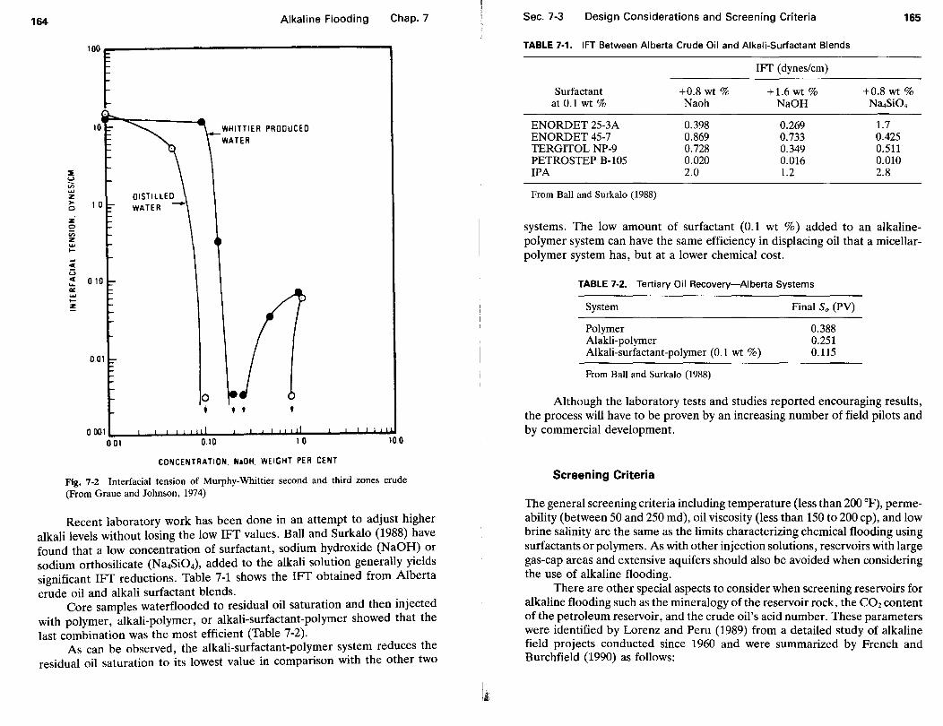
164
C(
u C( ... a:: .... ,_ z
0
Alkaline Flooding
WHITTIER PRODUCED WATER
• • •
CONCENTRATION. N10H. WEIGHT PER CENT
Chap. 7
Fig. 7-2 Interfacial tension of Murphy-Whittier second and third zones crude (From Graue and Johnson, 1974)
Recent laboratory work has been done in an attempt to adjust higher alkali levels without losing the low IFf values. Ball and Surkalo (1988) have found that a low concentration of surfactant, sodium hydroxide (NaOH) or sodium orthosilicate (Na4Si04), added to the alkali solution generally yields significant IFf reductions. Table 7-1 shows the IFf obtained from Alberta crude oil and alkali surfactant blends.
Core samples waterflooded to residual oil saturation and then injected with polymer, alkali-polymer, or alkali-surfactant-polymer showed that the last combination was the most efficient (Table 7-2).
As can be observed, the alkali-surfactant-polymer system reduces the residual oil saturation to its lowest value in comparison with the other two
I
li
Sec. 7-3 Design Considerations and Screening Criteria
TABLE 7-1. 1FT Between Alberta Crude Oil and Alkali-Surfactant Blends
Surfactant at 0.1 wt%
ENORDET 25-3A ENORDET 45-7 TERGITOL NP-9 PETROSTEP B-105 IPA
From Ball and Surkalo (1988)
+0.8 wt% Naoh
0.398 0.869 0.728 0.020 2.0
IFf (dynes/em)
+1.6 wt% NaOH
0.269 0.733 0.349 0.016 1.2
165
+0.8 wt% N14Si04
1.7 0.425 0.511 0.010 2.8
systems. The low amount of surfactant (0.1 wt %) added to an alkalinepolymer system can have the same efficiency in displacing oil that a micellarpolymer system has, but at a lower chemical cost.
TABLE 7-2. Tertiary Oil Recovery-Alberta Systems
System Final So (PV)
Polymer 0.388 Alakli-polymer 0.251 Alkali-surfactant-polymer (0.1 wt %) 0.115
From Ball and Surkalo (1988)
Although the laboratory tests and studies reported encouraging results, the process will have to be proven by an increasing number of field pilots and by commercial development.
Screening Criteria
The general screening criteria including temperature (less than 200 °F), permeability (between 50 and 250 md), oil viscosity (less than 150 to 200 cp ), and low brine salinity are the same as the limits characterizing chemical flooding using surfactants or polymers. As with other injection solutions, reservoirs with large gas-cap areas and extensive aquifers should also be avoided when considering the use of alkaline flooding.
There are other special aspects to consider when screening reservoirs for alkaline flooding such as the mineralogy of the reservoir rock, the C02 content of the petroleum reservoir, and the crude oil's acid number. These parameters were identified by Lorenz and Peru (1989) from a detailed study of alkaline field projects conducted since 1960 and were summarized by French and Burchfield (1990) as follows:

166 Alkaline Flooding Chap. 7
Gypsum. Reservoirs with gypsum (anhydrite) content greater than 0.1 percent should be rejected as candidates for alkaline flooding. The gypsum reacts and consumes the alkali agent. For instance, 1% gypsum in a reservoir can consume 10 PV of a 1 percent solution of NaHC03.
Kaolinite. Reservoirs that contain appreciable amounts of kaolinite could be candidates for alkaline flooding only with low-pH (about 8.2-10) alkalis. The presence of kaolinite is a serious deterrent to flooding with higher-pH alkalis (Thornton, 1986).
Montmorillonite. The montmorillonite content of rock reservoir, because of its large surface area and very high cation exchange capacity, can consume much of the injected alkali by adverse precipitation reactions (Smith, 1978). Reservoirs with a montorillonite content higher than 1 percent and 0.4 wt % divalent ions in the brine are not good alkaline flooding candidates.
Sandstone. Sandstone reservoirs are preferred. High-pH alkalis are reactive with limestone.
Crude oil. It is important for the crude oil to have a high acid number* to achieve low 1FT in alkaline flooding, when the system does not include synthetic surfactant. However, even with crude oil with a low acid number, the alkaline flood can still be successful as a result of mechanisms other than 1FT lowering. The detailed study of alkaline field projects mentioned earlier did not show a correlation between oil acid number and project success (French and Burchfield, 1990).
Carbon dioxide. The C02 content of a petroleum reservoir is now considered a strong screening criteria parameter. Reservoirs with high C02 content, mole fraction of C02 (in produced gas) higher than 0.01, or a pH less than 6.5 are not good candidates for alkaline flooding (Lorenz and Peru, 1989).
7-4 FIELD TRIALS
Although more than 50 alkaline flooding field projects have been tested in the United States in the past 60 years, the method is not yet feasible as a commercial-scale operation (French and Burchfield, 1990). Two field trials of caustic flooding (Whittier oil field and Wilmington Ranger zone, California), where the published field results were combined with laboratory data, are presented next.
• Acid number is the number of milligrams of potassium hydroxide required to neutralize 1 gram of crude oil to pH = 7.0.
Sec. 7-4 Field Trials 167
Whittier Oil Field, California, United States
This field had been under a waterflood in progress when an experimental alkaline injection was initiated in 1966. The results were published by Graue and Johnson in 1974.
Reservoir characteristics. The project was started as a simultaneous flood in both productive second and third zones of the 63-acre project area at an average subsea depth of 1500 ft and 2100 ft, respectively. Other reservoir and fluid characteristics were
Net oil sand thickness Average porosity Air permeability Formation dip Oil gravity Reservoir temperature Oil viscosity Well spacing Permeability variation
37 ft and 100 ft 30%
495 md and 320 md 25° to 45° south 20 °API 120 °F 40 cp
1 and 2 acres per well 0.66 to 0.74
Project implementation. Approximately 1.6 million bbl of a solution composed of 20 percent PV of 0.2 wt % sodium hydroxide in water were injected through four initial injectors over a period of 10 months. The concentration of0.2 wt% NaOH is within the range which corresponds with the lowest interfacial tension value, Figure 7-2.
Results. Production data are shown in Figure 7-3, and as we observe, the caustic flood produced more oil than could have been expected from the continuation of waterflood. The response to caustic flooding showed drops in WORs also. However, this effect was exaggerated by shutting in a high-volume water producer near injector 135.
Comments. What is interesting to point out is that the injectors were located upstructure (Figure 7-4). A high-dip oil reservoir with a very good permeability exhibits a strong gravitational effect even when the crude oil viscosity is 40 cp. When the reservoir is moderately to highly heterogeneous, there are high permeability layers, referred to as thief channels, through which the gravitational flow of fluids rapidly reaches the downstructure producers.
.. ln~ee~, tracers were detected a short time (8 to 16 days) after the start of lfiJeCtiOn mto downstructure producers, and injection into Wells 75 and 135 was stopped.
The alkaline flood injection was started upstructure, probably to avoid
'

~
en co
~--'"--
,
~
m
1200r-----.------.------r------r-----.------r------r-----.------~-----r----~
1000
400
200 WATER INJECTION BEGAN
1963 1964
OIL PROOUCTION
~
CAUSTIC INJECTION
L. ' ' .., 1961 1966 1967 1968 1969 1970 1971 1971 1973
Fig. 7-3 Production data for wells in caustic flood area (From Graue and Johnson, 1974)
@denotes wells <·ompleted m upper zone area
Fig. 7-4 Wells in field trial area (From Graue and Johnson, 1974)
0
0
N
"'
12000
10000
ii: 8000 z'
c ;::: u :::> c
6000 ~ .. c
~ 4000 ~
~ .. .... ::
2000
0

170 Alkaline Flooding Chap. 7
the high water saturation existing downstructure where the w~terflood was supposed to take place. Nevertheless, it is ver.y important to cons1~er ca~efully the reservoir geometry and recovery mechamsms so that the way m whtch the new method is implemented will give maximum benefit.
Wilmington Field Ranger Zone, California, United States
The alkaline demonstration pilot project is comprised of two rows of four injectors each, which enclose the Block 9 pattern ~rea in t~e Ranger Z?ne of Wilmington Field. There are two reasons why alkal~n~ floodmg ~as constdered for Wilmington-the first is the low recovery eff1c1ency obtamed by waterflooding a reservoir which has permeability variations .and .an _unfavorable mobility ratio; the second was the high conte.nt of o~gamc act.ds m the crude oil. The injection was started in the 91 acres pilot proJect area m January 1979 with 10.2 percent PV softened freshwater with 1 percent added salts, followed by 67 percent PV of alkaline solution (0.39 wt % sodium orthosilicate) an~ by a postflush of softened water with 0.75 percent added salts. A very detailed study was published by the U.S. Departme~t of En~rgy.(Daube eta~., 1987) regarding the reservoir description and proJect destgn, 1mp~eme~tat10n, and results evaluation. The main results of this study are descnbed m the paragraphs that follow.
Reservoir characteristics. The productive formation lies at a depth of 2225 to 2800 ft and consists of six to eight intervals or subzones of 305 ft total average thickness of interbedded shales and unconsolidated to semiconsolidated sands. The main reservoir and fluid characteristics in the alkaline pilot area are
Average net thickness of subzones Average porosity between Average permeability between Average oil gravity, 0 API Bottom hole temperature Average oil viscosity
between 26 and 52 ft 0.246 and 0.289 131 md and 314 md 15-18, 16-23, 18-26, 20-28 125 °F 23 cp
Laboratory work. Detailed laboratory studies were performed using core samples recovered in frozen plastic pipe. Special core analysis tests showed an average displacement efficiency with waterflood of 4?·~ pe~cent of the oil in place and a cation exchange capacity from 2.6 to 1~.5 mt.lheqmvalents per 100 grams. The acid number of Ranger Zone crude ml vaned .from 0.~6 to 2.5 milligrams of KOH per gram of oil and measureme~t~ of mterfac~al tension indicated a lower value obtained with sodium orthosdtcate than w1th
Sec. 7-4 Field Trials 171
sodium hydroxide. The consumption tests performed showed alkali consumption ranged from 8.6 to 16.9 milliequivalents of alkali per 100 grams of rock at reservoir temperature and over a test period of 36 days. The reservoir contained a significant amount of clays and also gypsum. The laboratory displacement tests with alkaline solution indicated an average incremental recovery over waterflooding of about 6 percent of OOIP. The concentration of ions in the produced water suggested that during alkaline waterflooding the alkali was consumed and the core material was undergoing dissolution.
Simulation. A simulator model with the ability to represent the effects of the alkaline fluids by changes in the relative permeabilities was used in a one-dimensional form to simulate laboratory tests, a two-dimensional form to represent a limited area of the field, and a three-dimensional form to represent the entire project (Dauben et al., 1987). The pilot area simulation (three-dimensional model) predicted an incremental oil recovery of about only 1.9 percent of OOIP compared with 7.25 percent of OOIP predicted from the smaller two-dimensional pattern. This disappointing result appears to be the effect of the long-term consumption of alkaline fluids and of the larger surface area.
Minifield test. A two-month, one-well injectivity test was conducted before the start of the full scale pilot and satisfactory results were obtained regarding fluids injectivity and the operation of the surface facilities in handling the chemicals.
Project implementation. The alkaline slug injection started in March 1980. After the 10.2 percent PV preflush injection, 49,927,000 bbl (67 percent PV) of alkaline solution were injected over a period of 34 months at an average rate of 30,000 bbl/day.
Scale deposition. Scale deposition in producing wells after the breakthrough of alkaline solutions has been a major problem. Numerous workovers were conducted to overcome the plugging effects of scale in producing wells. The scales composed of calcium carbonate, magnesium silicate and amorphous silica were treated with a combination of acid and scale inhibitor injections.
Evaluation of results. The performance of the Block 9 pattern area is shown in Figure 7-5. As we can observe, the alkaline solution injection did not seem to have an impact on production data. The reduced injection rates after mid-1984, caused by the shutdown of two injection wells for repair, along with scale problems in producing wells, were responsible for the decline in gross oil production. The water-oil ratio did not appear to be practically influenced, although a reduced water production was observed in some of the wells. The plot, since 1976, of the oil cut versus cumulative oil recovery indicates that there

.. .. .. ... . . . Aeo;e Jqs uo!Pa[u 1 0
0 0 ------·HOI\ 0 0 0 0
o' q o. 0
Ll) N Ll) N
' I
" : · ..
I
: / ' " I
' : -:-'
\
" \ ( I
{ )
• , I
( <~:-.
I )
~ ~ \
... ~
'l ..... ) / ....
~ :
:
\
~ .... '\
,{ ' ... II '
/ .·· ...,
J D \
I
0 0 0 0 0 0 o. o. o. 0 0 0
- -·- Aeo;etqs t!O
-- Aeote Jqs ssoJ8
172
Ll)
co Cl>
r::::-<;t ao co a-en --;i
M 0 co "' en 0
.D ::l <II
Q N E co 0 Cl> e
a-- ~ u co 0 en :0
~ u "' '§ "'
0 >- 0 co "' en 0
u 0 .... 0 Oil
Cl> "' ...... "" en ~ <II ~ "1:1
co "' ...... 0 en 'B
::l "1:1 0
...... ~
...... en
~ -~
"" ... ...... en
0 0
lj 11
Chap. 7 References 173
was no improvement in oil recovery compared to waterflooding. The high consumption of chemicals and the wellbore plugging problems were the main reasons this project proved to be unsatisfactory, not to mention the lower than expected oil recovery (Dauben et al., 1987) .
Comments. The Wilmington Field Ranger Zone alkaline flood project is an example of how a very-well-prepared, developed, and executed project still did not produce the expected results in the field. It is very important to evaluate the complex reactions of alkaline chemicals with the reservoir rock and fluid content. Even so, losses from chemical consumption observed in laboratory tests, when transferred to the field scale, can be the main reason for failure. Another important aspect is reservoir geometry. The Ranger Zone consists of several subzones separated by impermeable shale barriers. Even if these shale barriers are continuous, they are in hydrodynamic communication through the producers, each opening up at least six subzones. A selective injection schedule starting with the lowest continuous subzone possibly could have been prepared, controlled, and evaluated with less rock surface exposed to chemical reactions.
QUESTIONS AND EXERCISES
7-1 Enumerate the mechanisms suggested for oil displacement by alkaline flooding and explain the differences .
7-2 Describe what can be done to adjust higher alkali levels without losing low IFf values.
7-3 Enumerate and explain the special aspects to consider as screening criteria for alkaline flooding.
7-4 What are the merits of the two alkaline field trials-Whittier Oil Field and Wilmington Ranger Zone?
REFERENCES
BALL, J., and H. SURKALO, "New Variations of Chemicals EOR and Their Economic Potential: The ASP Process (Alkaline-Surfactant-Polymer)," Proceedings of the Improved Oil Recovery Conference, Abilene, Texas, September 1988 (U.S. Department of Energy, DOE/BC/14286-1, March 1989), pp. 229-50.
COOKE, C. E., R. E. WILLIAMS and P. A. KOLODZIE, Journal of Petroleum Technology, (December 1974), p. 1365.
CRAIG, F. F., The Reservoir Engineering Aspects of Waterflooding, third printing (Richardson, TX: Society of Petroleum Engineers, 1980), pp. 12-17.
DAUBEN, D. L., R. A. EASTERLY, and M. M. WESTERN, An Evaluation of the Alkaline Waterflooding Demonstration Project Ranger Zone Wilmington Field, California (U.S. Department of Energy, DOE/BC/10830-5, May 1987).
'
174 Alkaline Flooding Chap. 7
FRENCH, T. R., and T. E. BURCHFIELD, "Design and Optimization of Alkaline Flooding Formulations" SPE/DOE 20238, presented at the Seventh Symposium on Enhanced Oil Recovery, Tulsa, Oklahoma, April 22-25, 1990.
GRAUE, D. J., and C. E. JOHNSON, JR., "Field Trial of Caustic Flooding Process," Journal of Petroleum Technology (December 1974), pp. 1353-58.
JENNINGS, H. Y.,JR., C. E. JOHNSON, and C. D. McAULIFFE, "A Caustic Waterflooding Process for Heavy Oils," Journal of Petroleum Technology (December 1974), pp. 1344-52.
JOHNSON, C. E., JR., "Status of Caustic and Emulsion Methods," Journal of Petroleum Technology (January 1976), pp. 85-91.
LORENZ, P. B., and D. A PERU, "Guidelines Help Select Reservoirs for NaHC03
EOR," Oil and Gas Journal (September 11, 1989), pp. 53-57.
MUNGAN, N., "Certain Wettability Effects in Laboratory Water Floods," Journal of Petroleum Technology (February 1966), pp. 247-52.
SMITH, F. W., "Ion-Exchange Conditioning of Sandstone for Chemical Flooding,;' Journal of Petroleum Technology (June 1978), pp. 959--68.
SQUIRES, F., "Method of Recovering Oil and Gas," U.S. Patent #1,238,355 (1917). SUBKOW, P., "Process for Removal of Bitumen from Bituminous Deposits," U.S. Patent
#2,288,857 (1942).
SURKALO, HARRY, "Enhanced Alkaline Flooding," Journal of Petroleum Technology (January 1990), pp. 6-7.
THORNTON, S.D., Reaction of Sodium Hydroxide with Silicate Minerals (U.S. Department of Energy, Report No. NIPER-129, N-115, April, 1986).
' J
Chapter 8
Miscible Fluid Displacement
8-1 GENERAL
As far back as 1927 Uren and Mahonay showed the existence of a relationship between oil recovery and the presence in the reservoir of interfacial tension among reservoir fluids. A substantial amount of oil (an average of66 percent of OOIP) remains in the reservoir after water or gas injection. The remaining oil is trapped as a discontinuous phase in the swept zone or forms a continuous phase in the unswept zone of the reservoir. The oil is trapped due to capillary forces and interfacial tensions and remains trapped regardless of how many pore volumes of water or low pressure gas are injected into the reservoir. Only by injecting a miscible agent which reduces the retaining forces to zero is nearly total displacement possible in the pores contacted by the miscible agent.
Miscible oil displacement is the displacement of oil by fluids with which it mixes in all proportions without the presence of an interface, all mixtures remaining single phase.
Beginning in the early 1950s and continuing into the 1960s, hydrocarbon fluids and alcohol were recommended as miscible agents and some were developed and field tested.
175

176 Miscible Fluid Displacement Chap.8
Propane, LPG mixtures, and low-molecular-weight alcohols were the solvents extensively investigated in the laboratory and in field tests. Many limiting factors such as high costs, unfavorable mobility ratios, and low volumetric sweep efficiencies restricted their full development. Even if small slugs of solvent were injected, driven through the reservoir with natural gas or with brine in the case of the alcohol slug, dilution and fingering of the solvent into the oil reduced their effectiveness.
Natural gas, flue gas, and nitrogen at high pressure and enriched hydrocarbon gas were found to achieve miscibility with the reservoir oil. High injection pressures and the composition requirement for miscibility of enriched gas limit the number of prospective oil reservoirs where this process of miscible fluid displacement can be used. Slugs of fluids containing oil, water, surfactants, and cosolvents (alcohol) in various formulations are known as micellarpolymer (MP) solutions. These were found to be technically efficient, resulting in initial miscibility and ultralow interfacial tension (IFf) further from the injection area. A favorable alternate injection fluid for increasing oil recovery is C02. The C02 miscible process has two main advantages. A relatively lower operating pressure is required for C02 to reach miscibility with reservoir fluids than with other solvents, and C02 is widely available from naturally occurring underground sources.
In this chapter, after presenting the miscible displacement principle, miscible flooding with hydrocarbon solvents will be emphasized. Micellarpolymer flooding will be described in Chapter 9 and C02 miscible flooding in Chapter 10.
8-2 PHASE BEHAVIOR
Phase Change Representations
Review of state-of-the-art miscible displacement has been treated comprehensively by an SPE monograph (Stalkup, 1984). Also, solvent-crude oil properties, phase behavior, and interfacial tension are detailed in the work of Lake (1989).
The miscible displacement mechanism of the EOR processes is understood when the phase behavior of crude oil, water, and enhanced oil recovery (EO R) fluids is known. A phase is a homogeneous, physically distinct, mechanically separable portion of a material with a given chemical composition and structure (Barrett et al., 1973). Oil and water represent two distinct liquid phases. Ice cubes in a glass of water is a two-phase system (ice and water). Ice cubes, water, and the vapor above the glass is a three-phase system. Even two regions of a solid with different compositions or crystal structures represents two distinct solid phases. The number of components in a system is the number
j
Sec. 8-2 Phase Behavior 177
of different kinds of atoms or molecules. An alloy, such as steel, consisting of two elements (iron and carbon) has two components. Water, H20, is a compound (having two elements); however, there is but one component, namely, the water molecule. Oil is a complex multicomponent system in which the components are the molecules of methane, CH4, ethane, C2H6, propane, C3H8,
and so on. Thus, if the elements of the system always appear in the form of a compound, we count only the molecule as the component and not the elements themselves (Barrett et al., 1973).
As we observed in Chapter 3, the change from water phase to vapor (steam) phase is dependent on both temperature and pressure. A graphical representation of the corresponding values of temperature and pressure at which phase changes occur is called a pressure-temperature (P-T) or a phase diagram. Other useful methods for displaying phase behavior data are triangular or ternary diagrams and pressure-compositon (P-X) diagrams. The first two methods, P-T and ternary diagrams will be presented here. The third, (P-X) diagram for mixtures of miscible displacement fluids and reservoir oils, is more complex since the exact composition of a reservoir fluid is very difficult, if not impossible, to discern.
P-T Phase Equilibria Diagram
One-component system. The classic example of a one-component system is water. The P-Tphase diagram for water is given in Figure 8-1. The lines OC, OF, and OS represent corresponding temperatures and pressures where two phases coexist, respectively, as vapor-liquid, liquid-solid, and solid-vapor and are in equilibrium. At the critical point C liquid and vapor exist simultaneously in equilibrium. At a temperature higher than critical temperature 1;;, the substance cannot be liquified regardless of how much pressure is applied. The gaseous phase above the critical temperature is called a gas; below the critical temperature it is called a vapor. At the triple point 0-which occurs at a pressure of 4.58 mm of mercury or 0.0882 psi (0.608 kPa) and a temperature of 32.0136 °F (0.0075 °C)-the solid, liquid, and saturated vapor exist simultaneously (Betts, 1981). A phase diagram is of great practical importance because it allows us to predict the state of the system for any particular temperature and pressure.
Example 8-1. On the basis of information given in Figure 8-1, show that ice should float in water (Barrett et al., 1975).
SOLUTION
slope of OF = negative
For a given T, ice changes to liquid asp increases. This suggests that the volume of the ice decreases on melting because this would relieve pressure. Hence, ice is less dense than water and will float.
'

178 Miscible Fluid Displacement Chap. a
Fusion
c 3114 ---- Liquid
Gas
Vapor
Temperature oF
Fig. 8-1 Phase diagram for water
Multicomponent system. Compared to the one-component system where two phases coexist only along a P-T line, in a multicomponent system such as an oil reservoir's, two phases gas and liquid are present in an area enclosed by the P-T phase diagram. Figure 8-2 is the P-T phase diagram of a particular reservoir fluid. · As we observe, the area enclosed by the bubble point and dew point lines which meet at the critical point is the region in which both gas and liquid phases will exist. The maximum two-phase temperature is called the cricondentherm. The curves within the two-phase region show the percentage of the total hydrocarbon volume which is liquid for any temperature and pressure (Craft and Hawkins, 1959). Various types of reservoirs can be defined by the location of the initial reservoir temperature and pressure with respect to the two-phase region.
Let us consider a reservoir where the composition corresponds to the phase diagram given in Figure 8-2, initially at 300 oF (147.4 oq and 3700 psia (259 atm), point A. Assume that reservoirs containing the same hydrocarbon mixture are located initially at
Point B, or 180° F (81.4° C) and 3300 psia (231 atm)
' ! ·; 1
l
Sec. 8-2 Phase Behavior
Point C, or 75° F (23.6° C) and 3000 psia (210 atm) Point D, or 150° F (64.9° C) and 2000 psia (140 atm)
179
For each reservoir location the existing phases, initial and during production operations, and the reservoir type are defined with reference to the phase diagram (Table 8-1).
Initially, the existing phases are in
Reservoir A, gas; the point A lies outside the two-phase region above the dew point line. Reservoir B, gas; the point B lies the same as above and between the critical point temperature and the cricondentherm. Reservoir C, liquid; the point lies outside the two-phase region above the bubble line. Reservoir D, liquid and gas; the point lies within the two-phase region.
4000
3500
<(3000 iii IL . w ~2500 C/) C/) w 0:: IL
!!:2000 0 > 0:: w C/) w 0:: 1500
1000
IUBILE POINT OR
DISSOLVED GAS
RESERVOIRS
DEW POINT DR
RETROGRADE
GAS ·CONDENSATE RESERVOIRS
~ . 0
300 350
Fig. 8-2 Pressure-temperature phase diagram of a reservoir fluid (From Craft and Hawkins, 1959)
'

180 Miscible Fluid Displacement Chap.S
During production operations, the reservoir temperature remains constant and the pressure declines.
The existing phases are in
Reservoir A, Gas, as pressure declines along path A-A1. Reservoir B, Gas, until the dew point pressure is reached at 2545 psia, point B1. Gas and Liquid (condensate), below point B1 since a liquid condenses out of the gas up to a maximum volume of 10 percent, reached at 2250 psia, point B2• This is called retrograde condensation because declining pressure generally causes vaporization, not condensation. With the continuous decrease of reservoir pressure vaporization of the retrograde liquid occurs from B2 to B3. Reservoir C, Liquid (Oil), until the bubble point pressure is reached at 2550 psia, point C1. Oil and Gas, below point C1. since the gas evolves from solution, build up an equilibrium gas saturation and flow with the oil through the reservoir to the producers. Reservoir D, Oil and Gas, the oil zone is overlaid by a gas zone or gas cap.
TABLE 8-1. Reservoir Types Defined with Reference to Phase Diagrams
EXISTING PHASES
DURING PRODUCTION INITIAL INITIAL OPERATIONS LOCA- in TION RESER- in at the RESERVOIR
(T andp) VOIR RESERVOIR SURFACE TYPE NOTES
Gas Dry-gas reservoir No gas
condenses A Gas Gas
Gas+ liquid Wet (Rich)-gas Gas condenses (condensate) reservoir at the surface
B Gas Gas+ liquid Gas+ liquid Retrograde Gas condenses at (condensate) (condensate) gas-condensate the surface and
reservoir in the reservoir (retrograde)
c Liquid Oil+ gas Oil+ gas Oil reservoir A secondary gas cap is forming in the reservoir
D Liquid Oil+ gas Oil+ gas Oil reservoir Gas may +gas with initial condense at
gas cap surface; at surface and in the reservoir
Sec. 8-2 Phase Behavior 181
During production operations each reservoir's existing phases appear at the surface as follows:
A, Gas. If the temperature of the fluid produced through the well bore and into surface separators does not enter the two-phase region, the reservoir type in this case is a dry-gas reservoir. Gas and Condensate. If the fluid produced enters the two-phase region due to a temperature decline, as along line A-A2, the reservoir type is a wet- or rich-gas reservoir.
B, Gas and Condensate. This reservoir type is a retrograde gas-condensate reservoir. C, Oil and Gas. This reservoir type is an oil reservoir or dissolved (solution) gas-drive reservoir.
D, Oil and Gas. This reservoir type is an oil reservoir with initial gas cap.
Pressure-temperature diagrams are also useful for studying the miscibility behavior between a solvent and crude oil or between a solvent and dry gas.
Figure 8-3 shows a P-T diagram representing the vapor pressure curves of pure ethane (curve A C) and pure heptane (curve BC7 ). Curves A1 C1 Bh AzCzBz, and A3C3B3 trace the bubble and dew point curves for various mixtures of ethane and heptane. For instance, curve A2 C2 B2 represents a mixture containing 50.25 wt% ethane. The dashed line in Figure 8-3 connects the critical (plate) points for all mixtures of ethane and heptane. A constant temperature line representing reservoir conditions when pressure declines during production operations shows that all mixtures are single-phase above the dashed curve, whereas beneath this curve two phases, gas and liquid, may coexist, depending on the mixture composition (Stalkup, 1984).
Ternary Diagram
The ternary diagram represents, on an equilateral triangle, the phase behavior of a three-component mixture (Figure 8-4 ).
Each corner of the equilateral triangle represents one of the components (100 percent), and each side corresponds to zero percent of the component represented by the opposite corner. This simple three-component system has characteristics as follows (Stalkup, 1984):
• Mixtures can be plotted on the diagram. Thus, mixture A in Figure 8-4 contains 40 percent component 1, 20 percent component 2, and 40 percent component 3.
• A mixture with an overall composition given by point A is a two-phase mixture at a given pressure and temperature: an equilibrium gas phase (assuming component 1 is a gas) with composition y saturated with conden-
'
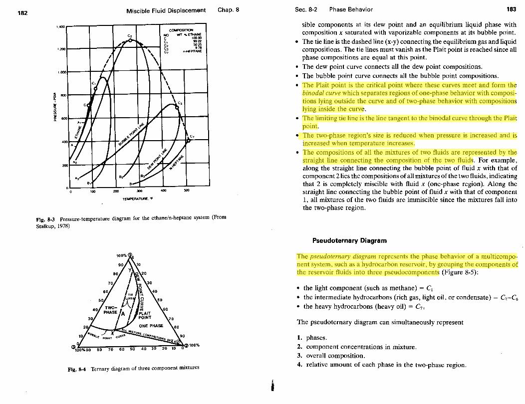
182 Miscible Fluid Displacement Chap. a
1.400 r----r---'T""--1--..,-------, C~TIOH
NO WT "'ETHANE c 10000 c, 9022
1.200~--+-----tJ~L-~~:"':'-1 g~ sg ~ c7 n-HEPTANE
oL--~~--~-~-L--~~--:500~-~ 0 100 200 300 400
TEMPERATURE. "F
Fig. 8-3 Pressure-temperature diagram for the ethane/n-heptane system (From
Stalkup, 1978)
Fig. 8-4 Ternary diagram of three component mixtures
Sec. 8-2 Phase Behavior 183
sible components at its dew point and an equilibrium liquid phase with composition x saturated with vaporizable components at its bubble point.
• The tie line is the dashed line (x-y) connecting the equilibrium gas and liquid compositions. The tie lines must vanish as the Plait point is reached since all phase compositions are equal at this point.
• The dew point curve connects all the dew point compositions. • The bubble point curve connects all the bubble point compositions. • The Plait point is the critical point where these curves meet and form the
binodal curve which separates regions of one-phase behavior with compositions lying outside the curve and of two-phase behavior with compositions lying inside the curve.
• The limiting tie line is the line tangent to the binodal curve through the Plait point.
• The two-phase region's size is reduced when pressure is increased and is increased when temperature increases.
• The compositions of all the mixtures of two fluids are represented by the straight line connecting the composition of the two fluids. For example, along the straight line connecting the bubble point of fluid x with that of component 2lies the compositions of all mixtures of the two fluids, indicating that 2 is completely miscible with fluid x (one-phase region). Along the straight line connecting the bubble point of fluid x with that of component 1, all mixtures of the two fluids are immiscible since the mixtures fall into the two-phase region.
Pseudoternary Diagram
The pseudoternary diagram represents the phase behavior of a multicomponent system, such as a hydrocarbon reservoir, by grouping the components of the reservoir fluids into three pseudocomponents (Figure 8-5):
• the light component (such as methane) = cl • the intermediate hydrocarbons (rich gas, light oil, or condensate) = C2-C6
• the heavy hydrocarbons (heavy oil) = c7+
The pseudoternary diagram can simultaneously represent
1. phases. 2. component concentrations in mixture. 3. overall composition. 4. relative amount of each phase in the two-phase region.

184 Miscible Fluid Displacement Chap.B
C7+ 100% C2-C
6 100%
Fig. 8-5 Pseudoternary diagram for a hydrocarbon reservoir
1. Phases. Let us assume that the hydrocarbon reservoir is a two-phase mixture which has an overall composition represented on the pseudoternary diagram (Figure 8-5) by point A. The corresponding tie line has
a. an equilibrium liquid phase S1 with composition x. b. an equilibrium gas phase S8 with composition y.
2. Concentrations. The component concentrations in the mixture are given in Table 8-2.
3. Overall Composition. The overall composition of the reservoir hydrocarbon mixture (point A) can be calculated based on each of the three pseudocomponents C~> C2_6, and C7+ and on the relative amount of the two phases S1 and S8 •
For example, the overall composition (point A) based on the pseudocomponent C1 is equal to the concentration of C1 in phase St multiplied by the
TABLE 8-2. Component Concentrations in Mixture
Concentration
Composition Phase c1 C2-6 c7+
X Liquid 0.20 0.20 0.60 A Liquid+ gas 0.50 0.15 0.35 y Gas 0.80 0.10 0.10
Sec. 8-2 Phase Behavior 185
relative amount of phase St plus the concentration of C1 in phase S multiplied by the relative amount of phase Sg. c
(8-1)
or based on
(8-2) and
(8-3)
4. Relative Amount. The relative amount of phases S1 and Sg can be found using Eqs. 8-1, 8-2, or 8-3 and Eq. 8-4:
St + Sc = 1
So, the relative amount of phase
sl = cl- cl,S - Cz-6- Cz-6,Sg = c7+ - c7+,S
CJ,s, - cl,Sg c2-6,s, - Cz-6,Sg C?+,s, - c7+,Sg
and, the relative amount of phase
s = cl - CJ,s, = c2-6 - c2-6,S, - c7+ - c7+,s,
g c!,Sg - CJ,s, c2-6,Sg - Cz-6,s, c7+,Sg - C7+,s,
(8-4)
(8-5)
(8-6)
Finding the relative amounts of phases Sg and S1 of the hydrocarbon mixture represented by point A suggests the use of the inverse lever rule (Lake, 1989). For example, if x represents 100 percent liquid phase S1 andy 100 percent gas phase Sg, the relative amount of phase S1 in the mixture represented by point A is the line segment between y and A divided by the length of the tie line between x andy.
S _line segment yA 1
- tie line xy and S = line segment xA 8 tie line xy
(8-7) .
where line segments and tie line are the differences between the concentrations based on each of the three pseudocomponents C1, C2_6, or C7+.
Example 8-2. Using the ternary diagram data given in Figure 8-5 and the data given in Table 8-2, find the relative amount of phases S8 and Sdor the hydrocarbon mixture which has an overall composition represented by point A.
SOLUTION
Equations 8-5 and 8-6 or the inverse lever rule state that
s = 0.50- 0.20 = 0.15- 0.20 = 0.35- 0.60-g 0.80- 0.20 0.10- 0.20 0.10- 0.60- 0·50
based on C, based on c2-6
based on c7+

186
or
Miscible Fluid Displacement
s~ = o.5o- o.8o = o.15- 0.10 = o.35- 0.10 = 0_50 0.20 - 0.80 0.20 - 0.10 0.60 - 0.10 based on C, based on
Cz-6 based on
c7+
s1 = 1 - S8 = o.5o
8-3 HYDROCARBON-SOLVENT MISCIBLE FLOODING
Residual Oil Saturation and 1FT
Chap. a
The objective of miscible displacement is to increase the oil recovery by reducing the residual oil saturation to the lowest possible value. Since residual oil saturation depends on the capillary number Nc,
where
Nc = UIJ-0'
(8-8)
u = superficial or actual velocity, ft/day, since only pores and not the full area conduct fluid, (u = v/<j>).
1J- = oil viscosity, cp 0' = interfacial tension, dynes/em
and since the residual oil saturation decreases when the capillary number increases (Figure 8-6), the interfacial tension should be reduced to its lowest value by injecting a slug of miscible solvent driven by natural gas until miscibility is achieved. Then, only one phase will result from the mixture of miscible fluids, with no interfaces and consequently no 1FT between the fluids.
The injection fluids that can achieve in-reservoir miscibility with reservoir fluids are so-called first-contact miscible and multiple-contact miscible fluids (Stalkup, 1984).
First-Contact or Direct Miscibility
The first-contact miscible injection fluids used are liquid petroleum gas mixtures. These solvents mix directly with reservoir oils in all proportions and the mixture remains single phase. The phase behavior required for achieving direct miscibility in ideal conditions can be illustrated on a pseudoternary diagram where LPG solvent is represented by C2_6, the driving gas of the solvent slug by C1. and the heavy hydrocarbons pseudocomponent by C7+ (Figure 8-7).
Sec. 8-3 Hydrocarbon-Solvent Miscible Flooding 187
~~-------------
-' 5
~ Q 10 en UJ II:
10-• ,o-• CAPILLARY NUMBER. ~
Fig. 8-6 Dependence of residual oil saturation on capillary number (From Stalkup, 1984)
As we observe, not only is LPG first-contact miscible with reservoir oil, but LPG diluted with C1 up to composition A is also directly miscible with reservoir oil. In fact, the miscibility between reservoir oil, LPG, and C1 is represented by the area of the triangle OC2_6 A, where OA is the line tangent to the binodal curve. Any higher proportion of C1 existing in composition A will move the line segment OA to intercept the binodal curve and pass through
Fig. 8-7 First-contact miscibility scheme

188 Miscible Fluid Displacement Chap. a
the two-phase region where the miscibility is lost. In reality, the phase behavior during miscible displacement of the oil by the solvent slug is more complex. As the solvent slug continues to pass through the reservoir it also mixes with the driving gas behind it. A dilution process starts which moves the composition profile to intersect the two-phase region where the direct miscibility is lost.
Multiple-Contact or Dynamic Miscibility
Multiple-contact miscible injection fluids are natural gas at high pressure, enriched natural gas, flue gas, nitrogen, and carbon dioxide. These fluids are not first-contact miscible and form two-phase regions when mixed directly with reservoir fluids. The miscibility is achieved by the mass transfer of components which results from multiple and repeated contact between the oil and injection fluid during the flow through the reservoir.
There are two processes through which dynamic miscible displacement can be achieved in the reservoir, namely, condensing gas drive and vaporizing gas drive (Stalkup, 1984). Both processes are related to the location of the reservoir oil's composition on a pseudoternary diagram with respect to the limiting tie line (the tangent line to the binodal curve through the Plait point).
Condensing gas drive process. The condensing gas drive process takes place when the reservoir oil composition "0" lies to the left of the limiting tie line PB (intermediates-lean crude oil) on the pseudoternary diagram and when the injected solvent, which is a mixture of natural gas ( C1) and intermediates ( C2_6), has a composition lying between A and B in Figure 8-8.
The miscibility results from the in situ transfer (condensation) of intermediate hydrocarbon ethane through butane from the solvent injected into the reservoir oil.
Assuming that natural gas with the minimum concentration of C2_6 (point B) is injected into the reservoir with oil composition "0," the mechanism of dynamic miscibility takes place as follows (Stalkup, 1984):
• The compositions of all mixtures of two fluids, after their first contact, are represented by the straight line OB, and most fall within the two-phase region.
• The resultant two-phase mixture is M1. and its tie line connects the equilibrium liquid phase composition L 1 with the equilibrium gas phase composition Gt.
• Further injection of solvent B contacts equilibrium liquid phase compbsition L1 and forms a new overall mixture M2 with an equilibrium liquid phase composition L2 and an equilibrium gas phase composition G2 •
• Continued injection of solvent B enriches the reservoir's overall mixtures M1. M 2, M3, ••• with more intermediate components C2_6• A transition zone is created along the bubble point curve with equilibrium liquid phase com-
Sec. 8-3 Hydrocarbon-Solvent Miscible Flooding 189
Fig. 8-8 Condensing gas driving miscibility scheme
positions L~> L2 , L3 , ••• until the Plait point P composition is reached and the reservoir oil becomes directly miscible with the injected solvent B.
It has to be pointed out that the reservoir oil is also contacted by the equilibrium gas phase compositions and a transition zone is established along the dew point curve from G~> G2 , ••• to the Plait point P where direct miscibility is achieved.
For a given solvent composition there is a minimum pressure called the minimum miscibility pressure (MMP) above which the dynamic miscibility can be obtained in a condensing gas drive process. Since the two-phase region size of a pseudoternary diagram is reduced when reservoir pressure is increased, lower concentrations of intermediates C2_6 in the injected solvent are needed to accomplish miscibility at higher reservoir pressures.
Vaporizing gas drive process. The vaporizing gas drive process takes place when the reservoir oil composition "0" lies on or to the right of the limiting tie line PB (crude oil reach in intermediates), and when the injected solvent has a composition lying to the left of the limiting tie line and also to the left of the tangent line OA (Figure 8-9).
The injected solvents used are natural gas at high pressure (the highpressure gas process), flue gas, nitrogen, and C02 • The miscibility is attained above a minimum miscibility pressure which has different values corresponding to the different gases injected and to different reservoir oil compositions. The mechanism of multiple-contact miscibility results from the in situ mass transfer through vaporization of intermediate hydrocarbon components from the reservoir oil into the injected gas.

190 Miscible Fluid Displacement Chap.8
Fig. 8-9 Vaporizing gas driving miscibility scheme
The C02 miscible flood is an EOR method commercially developed and, as we pointed out, is presented separately in Chapter 10. The vaporizing gas drive mechanism explained here uses natural gas C1 at high pressure as an injection solvent (Stalkup, 1984). Since natural gas is readily accessible, the process has been successfully developed in the field. Miscibility is achieved in much the same manner using nitrogen gas and flue gas.
• The injected high-pressure gas C1 in contact with the reservoir oil "0" vaporizes, or extracts some C2_6 hydrocarbons from oil. A gas phase G1
results, with intermediate hydrocarbons in equilibrium with the liquid phase 1,..1• The two-phase mixture has the overall composition M1•
• Further injection of gas C1 pushes the equilibrium gas G1 so that it contacts more fresh reservoir oil "0," extracts more intermediates, and reaches a new overall composition M2 • At the ends of the tie line are the equilibrium gas phase composition G2 which has more intermediate hydrocarbons and the equilibrium liquid phase composition L2.
• Continued injection of gas C1 causes G2 to contact more fresh reservoir oil "0," enriching the gas phase composition at the displacing front along the dew point curve from G2 to G3 and so on, until the Plait point P composition and direct miscibility is reached.
It has to be pointed out that the vaporizing gas drive method is not a slug process. The high-pressure gas itself serves as both solvent and drive gas (Stalkup, 1984). The continued injection of the high-pressure gas is the major difference between vaporizing gas drive floods and the majority of condensing gas drive and first-contact miscible floods.
Sec. 8-4 Field Development of Hydrocarbon-Solvent Flooding 191
The two mechanisms of dynamic miscibility just described (namely, transfer through condensation of intermediate components from rich solvent into the intermediates-lean crude oil, and transfer through vaporization of intermediate components from crude oil rich in intermediates into the solventlean gas at high pressure) are more complex in the fluid flow under actual reservoir conditions. However, the pseudoternary diagram behavior is very useful for recognizing the type of miscibility that can take place with various specific reservoir oil characteristics and solvent compositions.
8-4 FIELD DEVELOPMENT OF HYDROCARBON-SOLVENT FLOODING
The available data on field tests and development of miscible hydrocarbon displacement show the use of
• liquid petroleum gas as a first-contact miscible process. • enriched hydrocarbon gas as a multiple-contact condensing gas drive pro
cess. • high-pressure natural gas as a multiple-contact vaporizing gas drive process.
Beginning in the early 1950s and continuing into the 1960s and beyond, numerous field tests and several projects have been developed in the United States using LPG especially for miscible displacement.
However, the need for excessively large LPG slugs and the high market value of liquid propane made LPG injection economically unattractive. The use of enriched hydrocarbon gas and high-pressure natural gas processes has become more attractive in areas where there is no readily available market for the gas and in deep reservoirs where the high miscibility pressure can be achieved without approaching the parting pressure of the formation.
Several presentations of selected projects using hydrocarbon-solvent flooding are given by van Poollen (1980) and by Stalkup (1984), and recent technical papers containing valuable information regarding their design, implementation, and performance evaluation are available (Da Sie and Guo, 1988; Mazzocchi et al., 1988).
To illustrate reservoir and miscible slug characteristics and their accompanying operating strategies, some case histories are presented next.
Rainbow Keg River "B" Pool, Alberta, Canada
This is an example of a recently developed direct miscibility process using a tertiary first-contact hydrocarbon miscible flood (Mazzocchi et al., 1988).

192 Miscible Fluid Displacement Chap. 8
Reservoir characteristics. The reservoir is a reef of Middle Devonian age discovered in 1965 at 5900 ft (1800 m) and originally containing 272 million STB (43 million m3
) of a 38 °API (SG = 0.830) oil. The reefs geometry shows two structural lobes (north and south) separated by an east-west-oriented saddle and characterized by a 360ft (110m) formation maximum thickness. A geological and petrophysical model of the reservoir has been developed based on detailed studies and analyses of a large volume of cores, logs, three-dimensional seismic, reservoir, and production data. Within the original thick oil column, the formation above the oil-water contact was characterized as having a predominant limestone zone on the top with mainly vuggy and intergranular porosities and permeabilities; the formation below has two dolomite zones with good to excellent reservoir qualities as a result of the vuggs and fractures system.
Recovery mechanisms. Primary production resulted from fluid expansion drive until1968 since the reservoir saturation pressure of 1572 psig (10,845 kPa) was far below the initial pressure of 2465 psig (17 ,000 kPa). Water injection into the underlying aquifer started in 1969 and continued until1984. The oil-water contact rose 203 feet (61 m) in the northern lobe and 221ft (67 m) in the southern lobe, reaching a level above the saddle (Figure 8-10).
The oil recovery was approximately 37 percent of OOIP and the residual oil saturation range to waterflood was estimated for three petrophysical rock types at less than 0.25 for the vugular, fractured rock type 1, between 0.25 and 0.47 for rock type 2, with average porosities, and higher than 0.47 for tight matrix rock type 3.
SECONDARY SOLVENT FLOOD STARTED 82·03 110
100
90
80
70
TERTIARY SOLVENT FLOOD STARTED 84-06
Fig. 8-10 Rainbow Keg River B pool tertiary scheme. Average fluid levels (From Mazzocchi et al., 1988)
Sec. 8-4 Field Development of Hydrocarbon-Solvent Flooding 193
Secondary and tertiary miscible displacement. The reservoir geometry and characteristics were considered appropriate for direct miscible or first-contact miscible displacement using hydrocarbon solvent (LPG). The miscibility conditions and the design of the miscible flood were determined based on prediction made from miscibility correlation curves, visual cell phase envelope determinations, slim tube experiments, and core displacement studies. The pseudophase ternary diagram obtained (Figure 8-11) indicated that at 2200 psia (15,169 kPa) and 185° F (85° C) the minimum hydrocarbon solvent C2+ requirement of composition "S" was 57 percent to achieve first-contact miscibility with the reservoir oil of composition "0" (Mazzocchi et al., 1988).
Operating strategy. A solvent slug of 19.5 percent initial hydrocarbon pore volume injected in the crestal virgin zones of the reef and chased over with a pore volume of dry gas will spread horizontally across the top of the reef and will push about half of the mobilized oil down into the waterswept zone. The oil and solvent banks will form a tertiary common bank below the saddle that moves downward and displaces the residual oil. Water from the waterswept zone is simultaneously produced allowing the formation of the tertiary oil bank and the downward movement. The schematic representation of a tertiary miscible flood (Mazzocchi et al., 1988) is shown in Figure 8-12.
It is interesting to observe the original well completion techniques using sliding sleeves and packer combinations to control tertiary oil bank movement, water, oil and solvent production. The schematic representation of the recompletion strategy is shown in Figure 8-13. Four groups of perforation intervals are sequentially moved downward below the oil bank as the flood progresses (Mazzocchi et al., 1988).
RESERVOIR CONDITIONS
PRESSURE - 151811 kP• TEMPERATURE - 85°C
Cs+
FIRST CONTACT MISCIBILITY SOLVENT COMPOSITION
Fig. 8-11 Rainbow Keg River B pool ternary diagram (From Mazzocchi et at., 1988)

194
NORTHERN LOBE SOLVENT INJECTION
CONTINUES
OIL PRODUCTION
Miscible Fluid Displacement
SOUTHERN LOBE SOLVENT INJECTION
STARTED JULY 1, 11M
OIL PRODUCTION CURRENT
0/W CONTACT
WATER PRODUCTION
A.lililmll]·~ OIL PRODUCTION
SIX YEARS AFTER START OF TERTIARY SCHEME
ORIGINAL 0/W CONTACT END OF TERTIARY SCHEME
WATER PRODUCTION
~WATER SWEPT OIL ZONE VIRGIN OIL ZONE TERTIARY OIL BANK
rn SOLVENT BANK D CHASE GAS BANK
Chap. a
Fig. 8-12 Rainbow Keg River B pool tertiary scheme. Schematic representation of tertiary miscible flood (From Mazzocchi et a!., 1988)
The system provides control of the fluids being produced and of the downward displacement, minimizing drawdown and preventing coning of solvent and chase gas. The producing GOR and WOR values dictate the timing of opening and closing the perforations.
First results. Solvent flooding into the crestal zone of the northern lobe began in March 1982. The miscible flood into the crestal area of the southern lobe was started in June 1984. The total solvent injection corresponded to a
Sec. 8-4 Field Development of Hydrocarbon-Solvent Flooding
CURRENT~O~----~~------~ CONTACT PERFORATION
GROUP 1 '
I} ~ ~ERIOD 1984-19111
PERFORATION GROUP 2 PERIOD 1990-19114
II PERFORATION GROUP 3 II
PERFORATION GROUP 4 PERIOD 2000..2031
ORIGINAL 0/W CONTACT
T PERFORATION SUBGROUP 1
I PERFORATION SUBGROUP 2
I PERFORATION SUBGROUP 3
I PERFORATION SUBGROUP 4
Fig. 8-13 Rainbow Keg River B pool tertiary scheme. Schematic representation of recompletion strategy (From Mazzocchi eta!., 1988)
195
9.1 percent initial hydrocarbon pore volume (19.5 percent IHCPV was the projected solvent slug injection volume). As can be observed in Figure 8-14, oil production continued to decrease but at a slower rate than before. The water production increased as predicted and the gas production also increased after the breakthrough of solvent at the producers.
The cumulative solvent injected until June 1989 into the "B" pool amounted to 41,727 MMCF (1.175 x 10⁹ m3
), and the total amount produced was 7.9 MMCF, or 18.9 percent solvent recycled. The oil recovery increased to 43.8 percent of OOIP by the end of June 1987, compared with 37 percent
10000- 10000 10
~ c 0 ::-
=- 1000- ! 1000 E
~ a: 0 c:J
z 0 j: CJ :I 0
100-~ 100 0.1 A.
10-
Fig. 8-14 Rainbow Key River B pool production history (From Mazzocchi et a!., 1988)
-~ ! a: 0 311:
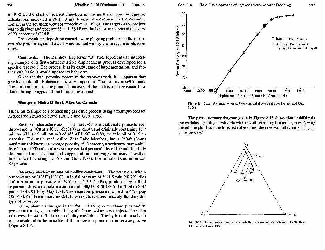
196 Miscible Fluid Displacement Chap.8
in 1982 at the start of solvent injection in the northern lobe. Volumetric calculations indicated a 26 ft (8 m) downward movement in the oil-water contact in the southern lobe (Mazzocchi et al., 1988). The target of the project was to displace and produce 55 x 106 STB residual oil or an increased recovery of 20 percent of OOIP.
The asphaltene deposition caused severe plugging problems in the northern lobe producers, and the wells were treated with xylene to regain production rates.
Comments. The Rainbow Keg River "B" Pool represents an interesting example of a first-contact miscible displacement process developed for a specific reservoir. The process is at its early stage of implementation, and further publications would update its behavior.
Given the dual porosity system of the reservoir rock, it is apparent that gravity stable oil displacement is very important. The tertiary miscible bank flows into and out of the granular porosity of the matrix and the easier flow fluids through vuggs and fractures is restrained.
Westpem Nisku D Reef, Alberta, Canada
This is an example of a condensing gas drive process using a multiple-contact hydrocarbon miscible flood (Da Sie and Guo, 1988).
Reservoir characteristics. The reservoir is a carbonate pinnacle reef discovered in 1978 at a 10,171-ft (3100 m) depth and originally containing 15.7 million STB (2.5 million m3
) of 45° API (SG = 0.80) volatile oil of 0.19 cp viscosity. The main reef, called Zeta Lake Member, has a 250-ft (76-m) maximum thickness, an average porosity of 12 percent, a horizontal permeability of about 1050 md, and an average vertical permeability of 100 md. It is fully dolomitized and has abundant vuggy and pinpoint vuggy porosity as well as brecciation fracturing (Da Sie and Guo, 1988). The initial oil saturation was 89 percent.
Recovery mechanism and miscibility conditions. The reservoir, with a temperature of 218° F (102° C) an initial pressure of 5911.5 psig (40,760 kPa) and a saturation pressure of 3966 psig (17,345 kPa), produced by a fluid expansion drive a cumulative amount of 530,000 STB (83,670 m3
) oil or 3.37 percent of OOIP by May 1981. The reservoir pressure dropped to 4693 psig (32,355 kPa). Preliminary model study results justified miscibly flooding this type of reservoir.
Using plant residue gas in the form of 15 percent ethane plus and 85 percent natural gas, a combined slug of 1.2 pore volumes was injected in a slim tube experiment to find the miscibility conditions. The hydrocarbon solvent was considered to be miscible at the inflection point on the recovery curve (Figure 8-15).
Sec. 8-4 Field Development of Hydrocarbon-Solvent Flooding 197
100
"C 95 e u
"' -~ 90 > a.
<'--! 85 ... "' c:-~ 80 0 u
"' a: ~ 75 "' 1: "' a. 70
r:=:J Experimental Results
0 Adjusted Predictions to Reflect Experimental Results
65~--~----~~--~----~----~--~----~----~----3400 3600 380 4000 4200 4400 4600 4800 5000
Displacement Pressure (Pounds Per Square Inch)
Fig. 8-15 Slim tube simulation and experimental results (From Da Sie and Guo, 1988)
The pseudoternary diagram given in Figure 8-16 shows that at 4800 psia the enriched gas slug is miscible with the oil on multiple contact, transferring the ethane plus from the injected solvent into the reservoir oil (condensing gas drive process).
c,
0 Reservoir Oil
Fig. 8-16 Termary diagram for reservoir fluid system at 4800 psia and 218 op (From Da Sie and Guo, 1988)

198 Miscible Fluid Displacement Chap. a
Field operations and results. The vertical hydrocarbon miscible flood was started in May 1981, and the total amount of gas injected by June 1987 was 13 billion scf (363 x 106 m3
). Cumulative oil production by June 1987 was 5 million STB (803,000 m3
) or 34 percent of OOIP. The determination of the solvent-to-oil interface in reservoir conditions was performed comparing pulsed neutron capture logs run before and after the start of the process and analyzing core samples obtained from a new well drilled in the area in early 1987. The results provided clear evidence of the existence of a miscible swept zone with an average residual oil saturation of 5 percent. The gravity-stable solvent-oil flat interface moving downward did not yet break through into the producing well effluent. The producers are perforated at the base of the reef (Figure 8-17) and the production rates are high (2800 bbVday or 450m3/day per well). The vertical displacement rate has to be below the gravity-stable critical rate to prevent viscous fingering of solvent into the oil. It is expected that gas breakthrough due to coning will begin when the solvent-oil contact is within 33 ft (10m) of the existing completion (Da Sie and Guo, 1988).
The Westpem Nisku D Reef condensing gas drive miscible process is applied as a vertical displacement of a highly saturated oil column. It appears to be very efficient and has the potential to reach a high oil recovery estimated at 84 percent of OOIP.
Block 31 Field, Texas, United States
This is an example of a vaporizing gas drive miscible flood using high-pressure gas injection (Herbeck and Blanton, 1961; Stalkup, 1984).
Reservoir characteristics. The reservoir is a Middle Devonian siliceous limestone formation at an 8400 ft (2561 m) depth, having a 350-ft (107-m) thickness and originally containing about 250 million STB (39.75 x 10⁶ m3) of
Producer Injector Producer
Main Reef
Fig. 8-17 Schematic cross section of the Westpem Nisku D Reef (Adapted from Da Sie and Guo, 1988)
Sec. 8-5 Screening Criteria 199
46o API (SG = 0. 797) and 0.2-cp viscosity volatile oil, at a 140° F reservoir temperature. The reservoir rock has 15 percent porosity, 1 md permeability, and an irreducible water saturation of 37 percent.
The miscible process. Since the reservoir was highly undersaturated, it was produced primarily by a depletion elastic drive. Beginning in 1952 hydrocarbon gas was injected and flue gas since 1966 through 24 gas injection wells into a 350-acre inverted nine-spot pattern at a pressure of 4200 psia (28,958 kPa) (miscibility pressure of 3500 psia) and at a rate of 135 MM scf/day total gas. Flue gas was produced by steam boilers and compressed to injection pressure. The boilers were fueled with natural gas, avoiding the use of purchased hydrocarbon gas.
The results. The results of the project are considered very good since the oil recovery is close to the predicted value of 60 percent of OOIP.
Hassi-Messaoud Field, Algeria
This is the largest vaporizing gas drive process in the world using high pressure lean gas multiple-contact miscible flood (Pottier et al., 1967).
Reservoir characteristics. The reservoir is a domal structure at an 11 ,000-ft (3353-m) depth with a 355-ft (108-m) average thickness of sandstone characterized by discontinuous intercalations of siltstone and clay beds. The original undersaturated oil in place was 23 billion STB (3657 x 106 m3) at an initial pressure of 7200 psi and a 245° F temperature. The rock reservoir has 6 to 10 percent porosity, and the variable permeability ranges between 10 and 180 md.
. . !he process and results. The process of gas injection began in 1964 by mJectmg 175 MM scf/day (4.9 x 10⁶ m3/day) lean gas and maintaining the reservoir pressure at 4500 psia, above the miscibility pressure of 3750 psia. Alternate gas-water injection was beneficial in retarding gas breakthrough and/or controlling GOR increase after gas breakthrough. The project was successful and profitable.
8-5 SCREENING CRITERIA
~ydrocarb_on-solvent miscible flooding can only be applied to certain types of ml reservmrs. The reservoir's characteristics are the screening criteria used to decide if a reservoir is a good candidate for hydrocarbon-solvent miscible flooding. Exceptions are to be expected since the project's profitability de-

200 Miscible Fluid Displacement Chap.8
pends on the economic factors prevailing ~t th~ time of .the flo?d. The guidelines for identifying potential ml reservmr candidates for the
first-contact miscible process, the condensing gas drive process, and the va?orizing gas drive process were well established by Stalkup (1984) and are gtven in the paragraphs that follow.
The Oil Viscosity and Gravity
The viscosity of the oil under reservoir conditions is perhaps the mos~ i~portant screening criterion since all three types of hydrocarbon-so.lvent mtscib~e processes work best with oil viscosities at 1 cp or less, espectally for honzontal floods. A practical upper viscosity limit may range between approximate!~? and 5 cp. The upper limit for gravity-stable floods depends on the reservmr s vertical permeability. . .
Crude oils with gravities above 30" API are most smted to fust-contact miscible and to condensing gas drive miscible processes. Volatile undersaturated crude oils, with an API gravity greater than 40o API and rich in intermediate-molecular-weight hydrocarbon components, are required for the vaporizing gas drive miscible process.
Reservoir Pressure and Depth
The injection pressure necessary to maintain the Il_linimun;t miscibility ~ressure required by the process must be below the formatl?n partl?g p~e.ssure m rese:voir. Since the first-contact miscible process reqmres a miSCibility pressure m the range of 900 psia to 1300 psia to operate above the miscibility pressure and below the parting pressure, the reservoir depth has to be between 1500 ft to 2500 ft. The condensing gas drive process requires pressures in the range of 1500 to 3000 psia and reservoirs with a minimum depth between 2000 ft and 3000 ft.
Vaporizing gas drive miscibility is achieved at high pressu:es of 3500 psia (minimum) and up to 6000 psia (maximum); thus the method 1s consequently restricted to deep reservoirs.
Reservoir Geometry
The direction of flow is important in all three types of hydroca~bon-solve.nt miscible processes. Better operating conditions and re~~l~s occur I~ reserv~Irs with substantial relief and high and uniform permeabihties, favonng gravitystabilized flooding. In horizontal reservoirs, vertical permeability has to be restricted to avoid or reduce gravitational segregation.
Chap.8 Questions and Exercises 201
Oil Saturation at Start of the Project
Hydrocarbon-solvent miscible methods reduce the residual oil saturation after waterflooding, and therefore are tertiary methods. In this case a minimum of 25 percent PV residual oil saturation at the start of the project is desirable. A higher percentage of oil in place at the start of the project will afford even better results. Some of the hydrocarbon-solvent miscible processes, particularly vaporizing gas drive, have been initiated in large and nonwaterflooded reservoirs as secondary EOR methods with good success to date.
High-Risk Factors
The project risk is increased by the presence of extensive fracturing, a gas cap, a strong water drive, or high permeability contrasts.
Although hydrocarbon-solvent miscible flooding has proven to be a technically effective EOR process, hydrocarbon injection fluids are in short supply and not practically available in the quantities required for large-scale oil field flooding in the United States (DOE, 1984). However, hydrocarbon miscible flooding with the vaporizing gas drive process using lean gas is attractive because lean hydrocarbon gas is available at relatively low cost and the produced gas can be compressed to miscibility pressure and reinjected.
QUESTIONS AND EXERCISES
8-1 Explain what miscible oil displacement means. 8-2 Enumerate some of the agents that will achieve miscibility with reservoir oil. 8-3 Describe, with reference to the P-T phase diagram given in Figure 8-2, the existing
phases-initial and during production operations--of the oil reservoir located at Pi = 2850 psia and T = 150° F.
8-4 Considering the pseudoternary diagram of Figure 8-5, find the relative amount of phases S1 and Sg for the hydrocarbon mixture with the overall composition C
1 = 40
percent, Cz-6 = 20 percent, C7+ = 40 percent. 8-5 Show where the reservoir oil composition should be located on the pseudoternary
diagram of Figure 8-18 to have first-contact miscibility with dry-gas composition A (Figure 8-18).
8-6 Determine the lowest Cz-6 wt % in gas composition to have direct miscibility with oil composition 01 (Figure 8-18).
8-7 Find the types of miscible processes possible with oil compositions 0~, 02
, and 03 at reservoir pressures p 1 and Pz (Figure 8-18).
8-8 Explain the vaporizing gas drive mechanism, and state the important difference between this method and the majority of condensing gas drive and first-contact miscible floods.
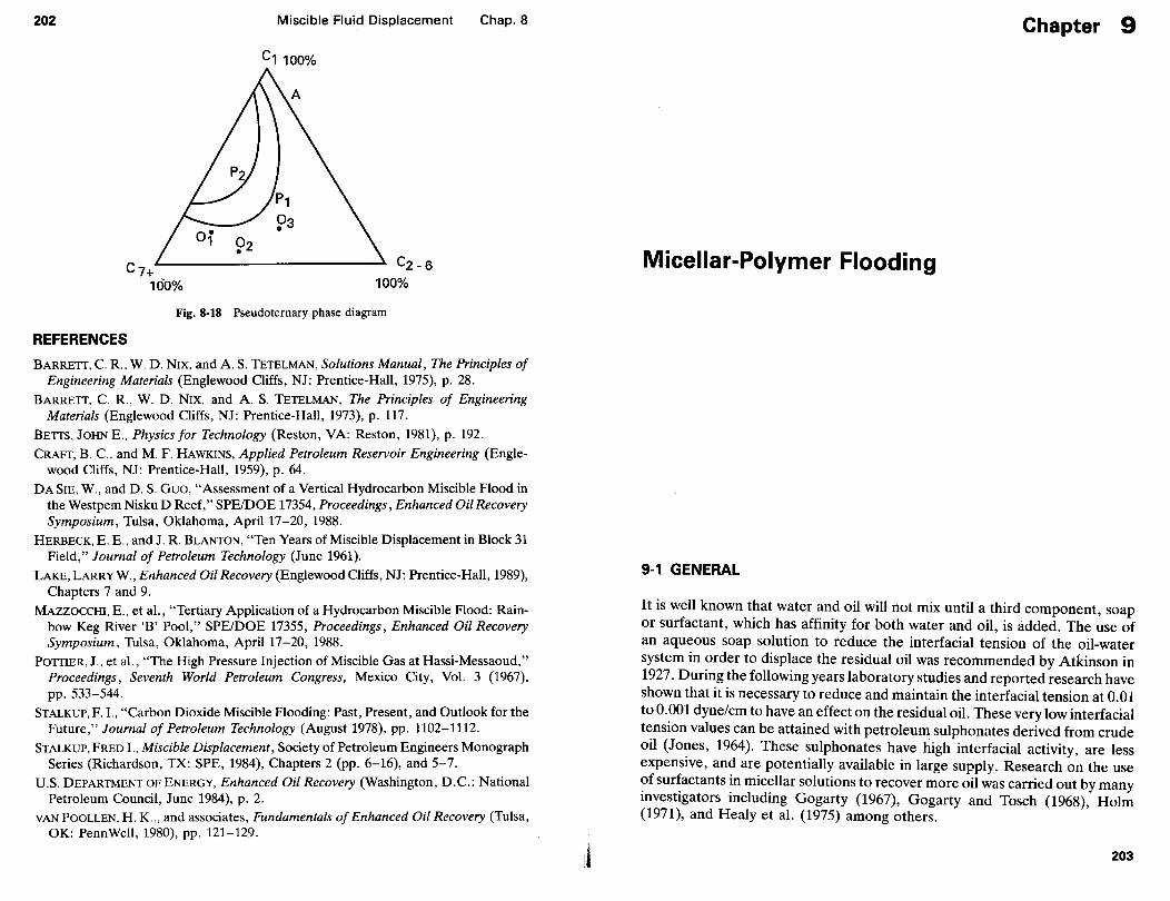
202
REFERENCES
Miscible Fluid Displacement
C110o%
c2- e 100%
Fig. 8-18 Pseudoternary phase diagram
Chap.8
BARRETI, C. R., W. D. NIX, and AS. TETELMAN, Solutions Manual, The Principles of Engineering Materials (Englewood Cliffs, NJ: Prentice-Hall, 1975), p. 28.
BARRETI, C. R., W. D. NIX, and A S. TETELMAN, The Principles of Engineering Materials (Englewood Cliffs, NJ: Prentice-Hall, 1973), p. 117.
BETIS, JOHN E., Physics for Technology (Reston, VA: Reston, 1981), p. 192.
CRAFT, B. C., and M. F. HAWKINS, Applied Petroleum Reservoir Engineering (Englewood Cliffs, NJ: Prentice-Hall, 1959), p. 64.
DA Sm. W., and D. S. Guo, "Assessment of a Vertical Hydrocarbon Miscible Flood in the Westpem Nisku D Reef," SPE/DOE 17354, Proceedings, Enhanced Oil Recovery Symposium, Tulsa, Oklahoma, April 17-20, 1988.
HERBECK, E. E., and J. R. BLANTON, "Ten Years of Miscible Displacement in Block 31 Field," Journal of Petroleum Technology (June 1961).
LAKE, LARRYW., Enhanced Oil Recovery (Englewood Cliffs, NJ: Prentice-Hall, 1989), Chapters 7 and 9.
MAZZOCCHI, E., et al., "Tertiary Application of a Hydrocarbon Miscible Flood: Rainbow Keg River 'B' Pool," SPE/DOE 17355, Proceedings, Enhanced Oil Recovery Symposium, Tulsa, Oklahoma, April17-20, 1988.
POTTIER, J., et al., "The High Pressure Injection of Miscible Gas at Hassi-Messaoud," Proceedings, Seventh World Petroleum Congress, Mexico City, Vol. 3 (1967), pp. 533-544.
STALK UP, F. I., "Carbon Dioxide Miscible Flooding: Past, Present, and Outlook for the Future," Journal of Petroleum Technology (August 1978), pp. 1102-1112.
STALKUP, FRED I., Miscible Displacement, Society of Petroleum Engineers Monograph Series (Richardson, TX: SPE, 1984), Chapters 2 (pp. 6-16), and 5-7.
U.S. DEPARTMENT OF ENERGY, Enhanced Oil Recovery (Washington, D.C.: National Petroleum Council, June 1984), p. 2.
VAN POOLLEN, H. K.., and associates, Fundamentals of Enhanced Oil Recovery (Tulsa, OK: PennWell, 1980), pp. 121-129.
Chapter 9
Micellar-Polymer Flooding
9-1 GENERAL
It is well known that water and oil will not mix until a third component, soap or surfactant, which has affinity for both water and oil, is added. The use of an aqueous soap solution to reduce the interfacial tension of the oil-water system in order to displace the residual oil was recommended by Atkinson in 1927. During the following years laboratory studies and reported research have shown that it is necessary to reduce and maintain the interfacial tension at 0.01 to 0.001 dyne/em to have an effect on the residual oil. These very low interfacial tension values can be attained with petroleum sulphonates derived from crude oil (Jo~es, 1964). These sulphonates have high interfacial activity, are less expenstve, and are potentially available in large supply. Research on the use ?f sur~actants ~n mic~llar solutions to recover more oil was carried out by many mvesttgators mcludmg Gogarty (1967), Gogarty and Tosch (1968), Holm (1971), and Healy et al. (1975) among others.
203
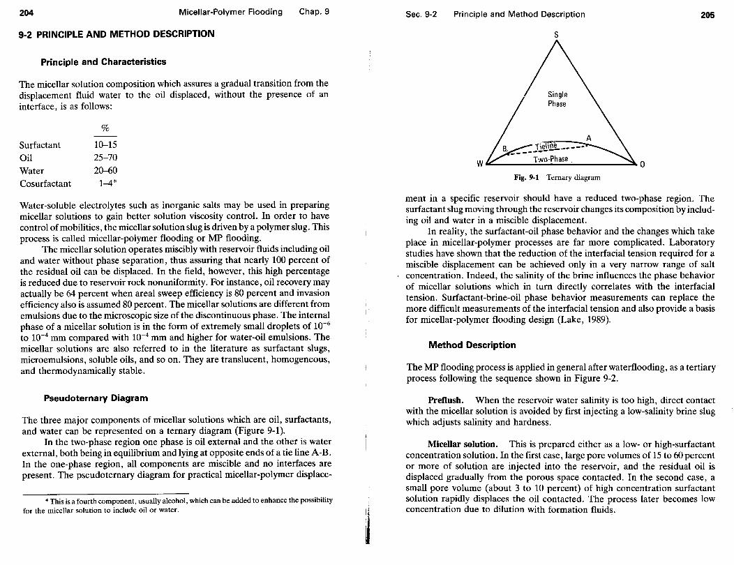
204 Micellar-Polymer Flooding Chap.9
9-2 PRINCIPLE AND METHOD DESCRIPTION
Principle and Characteristics
The micellar solution composition which assures a gradual transition from the displacement fluid water to the oil displaced, without the presence of an interface, is as follows:
%
Surfactant 10-15 Oil 25-70 Water 20--60 Cosurfactant 1-4*
Water-soluble electrolytes such as inorganic salts may be used in preparing micellar solutions to gain better solution viscosity control. In order to have control of mobilities, the micellar solution slug is driven by a polymer slug. This process is called micellar-polymer flooding or MP flooding.
The micellar solution operates miscibly with reservoir fluids including oil and water without phase separation, thus assuring that nearly 100 percent of the residual oil can be displaced. In the field, however, this high percentage is reduced due to reservoir rock nonuniformity. For instance, oil recovery may actually be 64 percent when areal sweep efficiency is 80 percent and invasion efficiency also is assumed 80 percent. The micellar solutions are different from emulsions due to the microscopic size of the discontinuous phase. The internal phase of a micellar solution is in the form of extremely small droplets of 10-6
to 10-4 mm compared with 10-4 mm and higher for water-oil emulsions. The micellar solutions are also referred to in the literature as surfactant slugs, microemulsions, soluble oils, and so on. They are translucent, homogeneous, and thermodynamically stable.
Pseudoternary Diagram
The three major components of micellar solutions which are oil, surfactants, and water can be represented on a ternary diagram (Figure 9-1 ).
In the two-phase region one phase is oil external and the other is water external, both being in equilibrium and lying at opposite ends of a tie line A-B. In the one-phase region, all components are miscible and no interfaces are present. The pseudoternary diagram for practical micellar-polymer displace-
• This is a fourth component, usually alcohol, which can be added to enhance the possibility for the micellar solution to include oil or water.
Sec. 9-2 Principle and Method Description 205
s
w 0
Fig. 9-1 Ternary diagram
ment in a specific reservoir should have a reduced two-phase region. The surfactant slug moving through the reservoir changes its composition by including oil and water in a miscible displacement.
In reality, the surfactant-oil phase behavior and the changes which take place in micellar-polymer processes are far more complicated. Laboratory studies have shown that the reduction of the interfacial tension required for a miscible displacement can be achieved only in a very narrow range of salt concentration. Indeed, the salinity of the brine influences the phase behavior of micellar solutions which in turn directly correlates with the interfacial tension. Surfactant-brine-oil phase behavior measurements can replace the more difficult measurements of the interfacial tension and also provide a basis for micellar-polymer flooding design (Lake, 1989).
Method Description
The MP flooding process is applied in general after waterflooding, as a tertiary process following the sequence shown in Figure 9-2.
Preflush. When the reservoir water salinity is too high, direct contact with the micellar solution is avoided by first injecting a low-salinity brine slug which adjusts salinity and hardness.
Micellar solution. This is prepared either as a low- or high-surfactant concentration solution. In the first case, large pore volumes of 15 to 60 percent or more of solution are injected into the reservoir, and the residual oil is displaced gradually from the porous space contacted. In the second case, a small pore volume (about 3 to 10 percent) of high concentration surfactant solution rapidly displaces the oil contacted. The process later becomes low concentration due to dilution with formation fluids.
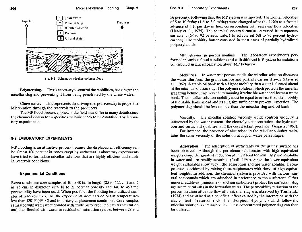
206 Micellar-Polymer Flooding Chap.9
Injector [IJ Chase Water
[}] Polymer Slug
(]] Micellar Solution
(D Preflush
[I] Oil and Water
Fig. 9-2 Schematic micellar-polymer flood
Producer
Polymer slug. This is necessary to control the mobilities, backing up the micellar slug and preventing it from being penetrated by the chase water.
Chase water. This represents the driving energy necessary to propel the MP solution through the reservoir to the producers.
The MP flood process applied in the field may differ in many details since the chemical system for a specific reservoir needs to be established by laboratory experiments.
9-3 LABORATORY EXPERIMENTS
MP flooding is an attractive process because the displacement efficiency can be almost 100 percent in zones swept by surfactant. Laboratory experiments have tried to formulate micellar solutions that are highly efficient and stable in reservoir conditions.
Experimental Conditions
Berea sandstone core samples of 10 to 48 in. in length (25 to 122 em) and 2 in. (5 em) in diameter with 18 to 21 percent porosity and 140 to 450 md permeability have been used. When possible, the flooding tests utilized samples of reservoir rock. All the experiments were carried out at temperatures less than 120° F ( 49a C) and in tertiary displacement conditions. Core samples saturated with water were flooded with crude oil to irreducible water saturation and then flooded with water to residual oil saturation (values between 28 and
Sec. 9-3 Laboratory Experiments 207
56 percent). Following this, the MP system was injected. The frontal velocities of 5 to 10ft/day (1.5 to 3.0 rn/day) were changed after the 1970s to a frontal advance of 1 ft per day or less, corresponding with reservoir flow velocities (Healy et al., 1975). The chemical system formulation varied from aqueous surfactant (68 to 92 percent water) to soluble oil (68 to 76 percent hydrocarbon). The mobility buffer consisted in most cases of partially hydrolized polyacrylamide.
MP behavior in porous medium. The laboratory experiments performed in various flood conditions and with different MP system formulations contributed useful information about MP behavior.
MQbilities. In water-wet porous media the micellar solution disperses the water film from the grains surface and partially carries it away (Davis et al., 1969). A stable oil bank with a higher mobility than water is formed ahead of the micellar solution slug. The polymer solution, which protects the micellar slug from behind, displaces the remaining irreducible water and forms a water bank. The micellar solution mobility must be equal to or less than the mobility of the stable bank ahead and its slug size sufficient to prevent dispersion. The polymer slug should be less mobile than the micellar slug and oil bank.
Viscosity. The micellar solution viscosity which controls mobility is influenced by the water content, the electrolyte concentration, the hydrocarbon and surfactant qualities, and the cosurfactant presence (Gogarty, 1968).
For instance, the presence of electrolyte in the micellar solution maintains the same viscosity of the solution at higher water percentages.
Adsorption. The adsorption of surfactants on the grains' surface has been observed. Although the petroleum sulphonates with high equivalent weights cau~e the greatest reduction in interfacial tension, they are insoluble in water and are readily adsorbed (Latil, 1980). Since the lower equivalent weight sulfonates show very little adsorption and are water soluble, a compromise is achieved by mixing these sulphonates with those of high equivalent weights. In addition, the chemical system is provided with various mineral compounds which are adsorbed in preference to the surfactant. Other mineral additives (ammonia or sodium carbonate) protect the surfactant slug against mineral salts in the formation water. The permeability reduction of the porous medium after the flow of a micellar slug was observed by Trushenski (1974) and explained as a beneficial effect caused by the interaction with the clay content of reservoir rock. The adsorption of polymers which follow the micellar solution is diminished and a less concentrated polymer slug can then be utilized.

208 Micellar-Polymer Flooding Chap. 9
9-4 FIELD TEST PROJECTS
The first micellar-polymer flood test was initiated in Dedrik Field, Illinois, in 1962. Despite industry interest the complexity of the method and its cost application restricted the number of field tests and the productive area involved. Two projects are described here: the largest conducted on 407 acres and started in 1977 by Marathon in the M-1 Field, Illinois, and the most successful pilot conducted in a 0.68-acre five-spot pattern by Exxon in the Loudon Field, Illinois, beginning in 1981.
The M-1 Project, Illinois, United States
The M-1 Project was a commercial-scale test of the Maraflood-enhanced oil recovery process. The Maraflood technique was developed by the Marathon Oil Company. It consisted of the use of water-oil microemulsions of which the discontinuous phase was in the form of droplets of microscopic size achieved by the use of a large percentage of a suitable surfactant and a certain amount of alcohol. The evaluation (Cole, 1988) and the final report (Stover, 1988) of the M-1 Project included project design and operations, production history, performance evaluation, and economic evaluation.
Reservoir characteristics. The oil reservoir is a Robinson sandstone characterized by a meandering stream deposition with a net average thickness of 27.8 ft at an average depth of 950ft. An average porosity of 18.9 percent and an arithmetic mean permeability of 103 md, with a Dykstra-Parsons permeability variation coefficient of 0.59 and 0.085 clay fraction content, characterize the rock reservoir. The oil viscosity is 7 cp and the reservoir water salinity is 16,575 ppm TDS.
The reservoir was developed to primary production under a dissolved gas drive mechanism from 1906 to 1941. The secondary recovery consisted of air repressuring (1941 to 1958) and was followed by waterflooding from 1958 to the start of the M-1 Project in 1976. The combined primary and secondary recovery averaged approximately 30 percent, and the most representative oil saturation at the start of the project was estimated to be 40 percent.
Project design. The scope of the project was to demonstrate economic recovery of tertiary oil in a mature waterflood project. The crude oil sulfonation/micellar-polymer technology used evolved from 15 years of field test experience with MP floods in the Robinson Sand (Cole, 1988).
The micellar slug design was based on the results of radial corefloods through k-in.-diameter "wellbores" formed in 2-in.-thick disks cut from 6-in.diameter cores in the project area. After cleaning and vacuum drying, the cores were resaturated with reservoir crude, waterflooded with synthetic brine to
I !
li
l
Sec. 9-4 Field Test Projects 209
residual oil, and injected with the micellar slug, mobility control buffer, and chase water. With the designed slug, recovery in the lab exceeded 70 percent of the residual oil after waterflooding in cores with permeability greater than 100 md.
In the field, 60percent of407 acres of the M-1 Project area was developed using 2.5-acre five-spot pattern spacing. The remaining area was developed with 5.0-acre pattern spacing.
The micellar-polymer fluid injection started in February 1977 (Cole, 1988) in the following sequence:
• The 10 percent pore volume micellar slug consisted of
Active sulfonate 10.0 wt% Inorganic salt 2.5 wt% Supply water 80.0 wt% Unreacted oil 7.5 wt%
The micellar slug was compatible with reservoir water so no preflush was needed. To prevent hydroxide precipitation of any iron in solution, 500 ppm of citric acid were added to the initial2000 bbl of injected slug. Cosurfactants added at the field site were hexyl alcohol 0.8 wt % and isopropyl alcohol 0 to 1.5 wt %.
• 105 percent pore volume of tapered mobility buffer (injection began in November 1978) consisted of partially hydrolized polyacrylamide in concentrations from 1156 ppm 11 percent, to 800 ppm 19 percent, 625 ppm 32 percent, 411 ppm 12 percent, 200 ppm 11 percent, 100 ppm 10 percent, and 50 ppm 10 percent. The polymer injection was completed in the 2.5-acre pattern area in August 1984 and in the 5.0-acre pattern area in 1989.
• 35 percent pore volume of produced water has to be injected until the injected fluids will total 1.5 pore volume.
Field Operations. Due to the advanced depletion of the reservoir, 101 of 114 injectors and 122 of 132 producers were drilled for the M-1 Project and were completed "open hole" through the productive formation. Extensive hydraulic fracturing with small fracture lengths was the most effective method of injection and production well stimulation. Treatment of the injectors with hydrogen peroxide was effective against the accumulation of concentrated or cross-linked polymer at sanqJace (Stover, 1988).
.-"?:
Production history. The graphs of the oil cut versus time for the 2.5-acre spacing area and for the 5-acre spacing area are shown in Figures 9-3 and 9-4, respectively.
As can be observed, the oil cut started to increase in the 2.5-acre spacing area in March 1979 after the injection of 18.6 percent PV and in the 5-acre
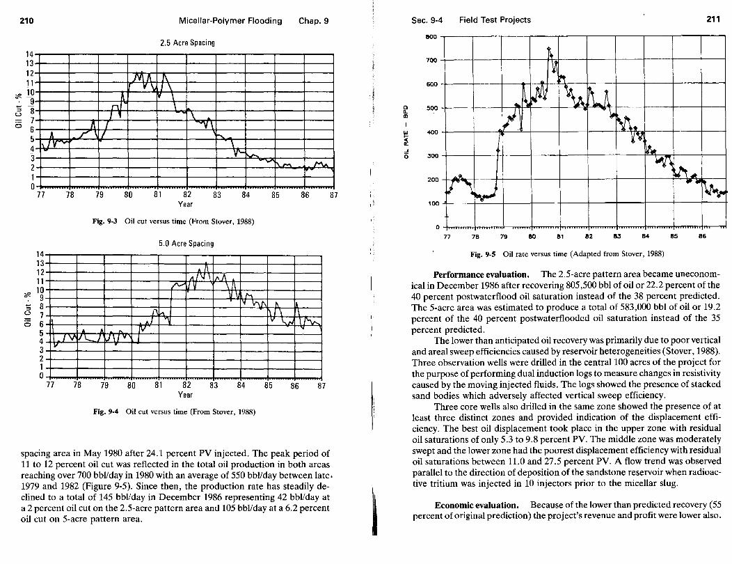
210
14 13 12 11
"*- 10 -9 -; 8 u ·- 7 0 6
A 5 4 3 2 1 0
I\ IV...,
77
14 13 12 11
"*- 10 9
-; 8 u 7 6 6
5 4 3 2 1 0
78
/V ...
~ n
I ' fl. I r\ I
79 80
Micellar-Polymer Flooding
2.5 Acre Spacing
N\1\ 1\ V\ I \
v \ \
81
\
82 Year
OVV\ h..
\ V'- ..-~
83 84 85
-
Fig. 9-3 Oil cut versus time (From Stover, 1988)
5.0 Acre Spacing
AI\ .... , \l \ "A
/'-"' l/ v \ 1\ V\J 1'-1 IV~ ~
111.-\ 1\1\ &-, '1 y \.,.,..
.t A .. IV V\.... 1 U\JV I
Chap.9
MA.
86
r\ I f'v.-. 'I
77 78 79 80 81 82 Year
83 84 85 86 87
Fig. 9-4 Oil cut versus time (From Stover, 1988)
87
spacing area in May 1980 after 24.1 percent PV injected. The peak period of 11 to 12 percent oil cut was reflected in the total oil production in both areas reaching over 700 bbl!day in 1980 with an average of 550 bbl!day between late. 1979 and 1982 (Figure 9-5). Since then, the production rate has steadily declined to a total of 145 bbl/day in December 1986 representing 42 bbllday at a 2 percent oil cut on the 2.5-acre pattern area and 105 bbl/day at a 6.2 percent oil cut on 5-acre pattern area.
j ..
\ ,.
0 D.. ID
I
~ ..J 6
Sec. 9-4 Field Test Projects 211
800
700 ~ ~
600
500
400
JOO
200
100
~ ....
4lo 1\~ 'U. l~ 11. ~
~t I ~~
~ ~ ~. ~
~\ ~ ... ~
0
n 78 79 80 81 82 83 84 85 86
Fig. 9-5 Oil rate versus time (Adapted from Stover, 1988)
Performance evaluation. The 2.5-acre pattern area became uneconomical in December 1986 after recovering 805,500 bbl of oil or 22.2 percent of the 40 percent postwaterflood oil saturation instead of the 38 percent predicted. The 5-acre area was estimated to produce a total of 583,000 bbl of oil or 19.2 percent of the 40 percent postwaterflooded oil saturation instead of the 35 percent predicted.
The lower than anticipated oil recovery was primarily due to poor vertical and areal sweep efficiencies caused by reservoir heterogeneities (Stover, 1988). Three observation wells were drilled in the central100 acres of the project for the purpose of performing dual induction logs to measure changes in resistivity caused by the moving injected fluids. The logs showed the presence of stacked sand bodies which adversely affected vertical sweep efficiency.
Three core wells also drilled in the same zone showed the presence of at least three distinct zones and provided indication of the displacement efficiency. The best oil displacement took place in the upper zone with residual oil saturations of only 5.3 to 9.8 percent PV. The middle zone was moderately swept and the lower zone had the poorest displacement efficiency with residual oil saturations between 11.0 and 27.5 percent PV. A flow trend was observed parallel to the direction of deposition of the sandstone reservoir when radioactive tritium was injected in 10 injectors prior to the micellar slug.
Economic evaluation. Because of the lower than predicted recovery (55 percent of original prediction) the project's revenue and profit were lower also.
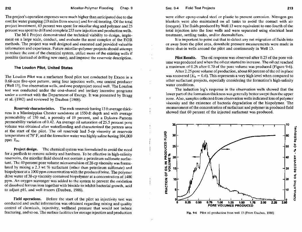
212 Micellar-Polymer Flooding Chap.9
The project's operation expenses were much higher than anticipated due to the cost for water pumping (10 miles from source) and for oil treating. Of the total project investment, 63 percent was spent for micellar slug and polymer and 25 percent was spent to drill and complete 233 new injection and production wells.
The M-1 Project demonstrated the technical viability to design, implement on a large scale, conduct, and evaluate the most complex of the EOR methods. The project was well designed and executed and provided valuable information and experience. Future micellar-polymer projects should attempt to reduce the cost of the chemical system, utilize more of the existing wells if possible (instead of drilling new ones), and improve the reservoir description.
The Loudon Pilot, United States
The Loudon Pilot was a surfactant flood pilot test conducted by Exxon in a 0.68-acre five-spot pattern, using four injection wells, one central producer (Welll3), five observation wells, and one postproject cored well. The Loudon test was conducted under the cost-shared and tertiary incentive programs under a contract with the Department of Energy. It was presented by Bragg et al. (1982) and reviewed by Dauben (1988).
Reservoir characteristics. The rock reservoir having 13 ft average thickness is a Mississippian Chester sandstone at 1550-ft depth and with average permeability of 150 md, a porosity of 19 percent, and a Dykstra-Parsons permeability variation of 0.42. An average oil saturation of 25.5 percent pore volume was obtained after waterflooding and characterized the pattern area at the start of the pilot. The oil reservoir had 5-cp viscosity at reservoir temperature of 78° F, and the formation water was highly saline having 104,000 ppm Tns·
Project design. The chemical system was formulated to avoid the need for a preflush to remove salinity and hardness. To be effective in high-salinity reservoirs, the micellar fluid should not contain a petroleum sulfonate surfactant. The 40 percent pore volume microemulsion of 28-cp viscosity was formulated by mixing a 2.3 wt % surfactant (other than petroleum sulfonate) and biopolymer at a 1000 ppm concentration with the produced brine. The polymer drive water of 38-cp viscosity contained biopolymer at a concentration of 1400 ppm. An oxygen scavenger was added to the system to prevent the oxidation of dissolved ferrous iron together with biocide to inhibit bacterial growth, acid to adjust pH, and well tracers (Dauben, 1988).
Field operations. Before the start of the pilot an injectivity test was conducted and useful information was obtained regarding mixing and quality control of chemicals, injectivity, wellhead pressure that would not induce fracturing, and so on. The surface facilities for storage injection and production
Sec. 9-4 Field Test Projects 213
were either epoxy-coated steel or plastic to prevent corrosion. Nitrogen gas blankets were also maintained on all tanks to avoid the contact with air (oxygen). The fluids produced by Well13 were equivalent to one-fourth of the total injection into the four wells and were separated using electrical heat treatment, settling tanks, and/or deemulsifiers.
It is important to point out that to detect any net migration of fluids into or away from the pilot area, downhole pressure measurements were made in three shut-in wells around the pilot and continuously in Well 13.
Pilot Results. The oil response was observed after 0.25 of the pore volume was produced and when the oil cut started to increase. The oil cut reached a maximum of 0.26 after 0.70 of the pore volume was produced (Figure 9-6).
After 2.25 pore volume of production, about 60 percent of the oil in place was recovered (ER = 0.6). This represents a very high level when compared to other surfactant projects, especially considering the formation's high-salinity water conditions.
The induction log's response in the observation wells showed that the lower part of the formation thickness was generally better swept than the upper zone. Also, samples collected from observation wells indicated loss of polymer viscosity and the existence of bacteria degradation of the biopolymer. The measurement of the concentration of surfactant and polymer in produced field showed that 60 percent of the injected surfactant was produced.
g 3 30 ~
Q
~ 25 ;:) 0 ~ ;#! 20 IlL~'~
z~ -;:) ...... sg 1s 1&. 0 z 0
~ : 1&.
70
0 2.00 2.26 2.&0
Fig. 9-6 Pilot oil production from well 13 (From Dauben, 1988)
_, « :::> Q (ii Yl a: ~
0
'# •
> cr: w > 0 u Yl cr:
= 0 100
~ ~ « ... :::> ~ :::> CJ

214 Micellar-Polymer Flooding Chap.9
Comments. The Loudon Pilot Test demonstrated the success of a special chemical system formulated for high-salinity formation brine conditions yet avoiding the need for a preflush. The next step to larger, semi commercialor commercial-scale production is possible since less surfactant is needed to penetrate to the producing well. The use of biopolymers will necessitate improved protection from microbial degradation. The Loudon Pilot is an example of how a very clear interpretation was possiblF when useful information was provided from sources such as core and well log analysis, interwell tracers, bottom hole pressure measurements, postproject wells cored, injection profile surveys, and others.
9-5 SCREENING CRITERIA AND CRITICAL QUANTITIES
Screening Criteria
Screening parameters for micellar-polymer flooding seem to reach a consensus. A given reservoir will be a micellar-polymer candidate if it is a sandstone, has a temperature of about 200° F or less, a permeability greater than 20 md, a residual oil saturation at the start of the project higher than 20 to 25 percent, and a formation water salinity of less than 200,000 ppm TDS, among other things. This screening approach is useful when considering the MP tertiary-enhanced recovery technique, for eliminating reservoirs that are technically unfeasible or have low economic potential.
For a large geological area or a particular country, it is very important to rank the reservoirs which pass all the criteria according to their EOR potential and estimated contribution to production. A preliminary economic evaluation program, PEOJ>N, was developed to identify first-rank reservoir candidates (Lake and Pope, 1979; U.S. Department of Energy, 1980; Paul et al., 1982). PEC<!>N has its limitations however, as it does not consider the time of oil breakthrough, the oil production versus time curve, and the time value of money. Another ranking system called the chemical flood prediction model (CFPM) was developed (Paul et al., 1982; Goldburg et al., 1983). The first step in the development of these models was to identify the critical reservoir and micellar quantities (CRMQ).
Critical Reservoir and Micellar Quantities
Based on an extensive volume of data from currently proposed, completed and ongoing MP/EOR field tests, the 29 quantities identified as affecting the micellar-polymer process were consolidated into 13 groups constituting the CRMQ (U.S. Department of Energy, 1980). These groups are
Sec. 9-5 Screening Criteria and Critical Quantities 215
1. Residual oil saturation and distribution. This is the oil saturation left behind by a pistonlike waterfront in the waterswept area. Its value and its distribution determine the amount of MP/EOR target oil and the high permeability zones, respectively. Higher residual oil saturation means more MP/EOR target oil but also a low permeability zone poorly swept by water.
2. Reservoir confinement. A given reservoir is a hydrodynamic unit characterized by confinement at reservoir boundaries and by continuity of the pay zone in the interior of the boundaries.
3. Natural fractures. As a system characterizing the reservoir rock is an unfavorable factor for an MP/EOR candidate reservoir. Induced fracturing in the injectors to increase injectivity can be beneficial.
4. Temperature and depth. Temperature is a limiting factor when trying to avoid mobility agent degradation, although IFf improves at elevated temperatures. Temperature is directly proportional to depth. This, in turn, controls the formation parting pressure.
5. Permeability and heterogeneity. It is important to know the areal and vertical distribution of permeability if possible. Evaluation of core sample analyses (Dykstra-Parsons coefficient) and the well's production-rate history may reveal vertical and areal flow trends.
6. PVT analysis of crude oil. The crude oil properties at reservoir conditions, especially the viscosity, are related to the design of the MP chemical system.
7. Makeup water composition. This represents total dissolved solids and total cations if full analysis is not available. The mobility buffer efficiency depends on the makeup water's composition for which the designation "fresh" is not sufficient.
8. Resident water composition. This is an important parameter to define since it determines the necessity for either an effective preflood or a chemical system tailored to the existing brine.
9. Relative permeabilities. These depend upon the microdistribution of fluids within the rock pores. This distribution is controlled by the rock wettability, which in turn, affects mobility requirements.
10. Pattern type and size. These seem to play an important role. There are indications that oil recovery is higher in the smaller pattern areas (Lowry et al., 1986).
11. Clay mineralogy and composition. These influence the surfactant adsorption, and an empirical link for this dependence might be established.
12. Rock mineralogy and composition. The level of carbonate minerals particularly affect the surfactant's electrolyte environment.
13. Volumetric waterflood data. This refers to the material balance equation which states that the original fluid in place equals the fluid produced plus the remaining fluid.
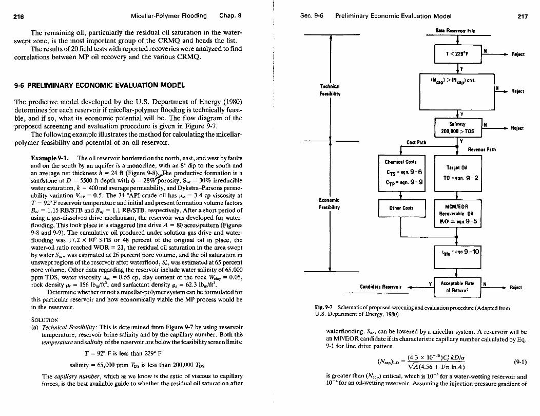
216 Micellar-Polymer Flooding Chap. 9
The remaining oil, particularly the residual oil saturation in the waterswept zone, is the most important group of the CRMQ and heads the list.
The results of 20 field tests with reported recoveries were analyzed to find correlations between MP oil recovery and the various CRMQ.
9-6 PRELIMINARY ECONOMIC EVALUATION MODEL
The predictive model developed by the U.S. Department of Energy (1980) determines for each reservoir if micellar-polymer flooding is technically feasible, and if so, what its economic potential will be. The flow diagram of the proposed screening and evaluation procedure is given in Figure 9-7.
The following example illustrates the method for calculating the micellarpolymer feasibility and potential of an oil reservoir.
Example 9-1. The oil reservoir bordered on the north, east, and west by faults and on the south by an aquifer is a monocline, with an 8° dip to the south and an average net thickness h = 24 ft (Figure 9-S~e productive formation is a sandstone at D = 5500-ft depth with <1> = 28% porosity, Sw; = 30% irreducible water saturation, k = 400 md average permeability, and Dykstra-Parsons permeability variation VDP = 0.5. The 34 °API crude oil has fLo = 3.4 cp viscosity at T = 92° F reservoir temperature and initial and present formation volume factors Bo; = 1.15 RB/STB and Bot = 1.1 RB/STB, respectively. After a short period of using a gas-dissolved drive mechanism, the reservoir was developed for waterflooding. This took place in a staggered line drive A = 80 acres/pattern (Figures 9-8 and 9-9). The cumulative oil produced under solution gas drive and waterflooding was 17.2 x 10⁶ STB or 48 percent of the original oil in place, the water-oil ratio reached WOR = 21, the residual oil saturation in the area swept by water Sorw was estimated at 26 percent pore volume, and the oil saturation in unswept regions of the reservoir after waterflood, S~, was estimated at 65 percent pore volume. Other data regarding the reservoir include water salinity of 65,000 ppm TDS, water viscosity ILw = 0.55 cp, clay content of the rock 'Wc1ay = 0.05, rock density p, = 156 lbm/fe, and surfactant density p, = 62.3 lbm/fe.
Determine whether or not a micellar-polymer system can be formulated for this particular reservoir and how economically viable the MP process would be in the reservoir.
SOLUTION
(a) Technical Feasibility: This is determined from Figure 9-7 by using reservoir temperature, reservoir brine salinity and by the capillary number. Both the temperature and salinity of the reservoir are below the feasibility screen limits:
T = 92° F is less than 229° F
salinity= 65,000 ppm TDs is less than 200,000 TDs
The capillary number, which as we know is the ratio of viscous to capillary forces, is the best available guide to whether the residual oil saturation after
Sec. 9-6 Preliminary Economic Evaluation Model
Technical Feasibility
Economic Feasibility
Cost Path
' Chemical Costs
crs=eqn.9-6
CTP = eqn. 9-9
+ Other Costs
IIISe R .. rvoir File
J T<229°F N
Jv (NCIP) > (NCip) crit.
r!-
1Y Sllinity N
200,000 > TDS
jv
l Revenue Path
Target Oil
TO =eqn. 9-2
f MCM/EOR
Recoverable Oil
P.O = eqn9-5
l f
tlife = eqn 9-10
'
217
Reject
Reject
Reject
te Reservoir y Acceptable Rate N
of Return? Candida Reject
Fig. 9-7 Schematic of proposed screening and evaluation procedure (Adapted from U.S. Department of Energy, 1980)
waterflooding, So, can be lowered by a micellar system. A reservoir will be an MP/EOR candidate if its characteristic capillary number calculated by Eq. 9-1 for line drive pattern
(N ) = (4.3 x w-10)C; kD!a
cap LD .... /"7 vA(4.56 + 1hr InA)
(9-1)
is greater than (Neap) critical, which is 10-5 for a water-wetting reservoir and 10-4 for an oil-wetting reservoir. Assuming the injection pressure gradient of

218 Micellar-Polymer Flooding Chap. 9
A
T ---------- ' 8 8 ............ ~ -500 ~ ~,
I · -5o5o-::::· ~ ~ 2 1 ~5100 -\ -\ 1 -----5150 .....\
~5200~ 0"" @) \
I _j__ \ A
Legend
-- contour intervals faults
0 producers I@ water Injectors
Fig. 9-8 Subsurface structural map scheme with waterflood pattern development
injector producers
\
Fig. 9-9 Structural cross-section scheme A-A'
C; = 0.5 psi/ft and the interfacial tension 3.33 X 10⁻³ dynes/em, the capillary number is
(Nca )w = 1.29 X 10⁻⁷(0.5)400 X 5500 = 2.67 X 10_3
P vSo( 4.56 + 1/TI In 80)
Not having available reservoir wettability data, the (Ncap)c, for water-wet media will be used:
field (Ncap)LD = 2.67 X 10⁻³ > 10-5 = (Ncap)cr
Since the reservoir meets temperature, salinity, and capillary number criteria, a chemical system can be designed that will mobilize residual oil.
Sec. 9-6 Preliminary Economic Evaluation Model 219
(b) Economic Feasibility: This is illustrated by calculating target oil, recoverable oil, surfactant and polymer requirements, project life, field development, cost data, and the revenue to expense ratio.
1. Target Oil. Target oil, TO, is defined as the oil remaining in the waterfloodswept portion of the reservoir at the start of the MP process. Using the same notations as in Appendix II of the 1980 U.S. Department of Energy report, the target oil is
TO = PV x Sorw Ev Bot
(9-2)
where the volumetric efficiency Ev is given by a material balance equation applied at the end of waterflooding, for one pore volume PV
original oil in place = remaining oil in place + oil produced
PV Soi = PV(1 - Ev) S~ + PV x Ev Sorw + Np (9-3) Boi Bot Bot
Solving (9-3) for Ev after replacing
gives
or
PV = OOIP x Bo; Soi
E = So;Bot1Bo;(1- NJOOIP)- S~ v Sorw- S~
E = 0. 7 X 1.111.15(1 - 0.48) - 0.65 = O 7738 v 0.26 - 0.65 .
and the target oil
TO= OOIP X Bo; x Sorw Ev = 17.2 X 106
X 1.15 x 0.26 x 0.7738 Soi Bot 0.48 X 0.7 1.1
= 10.767 x 10⁶ STB or
(9-4)
which can be expressed as 57.5 percent of the oil in place at the start of the process.
2. Recoverable Oil. Recoverable oil, RO, is estimated from the ratio
produced oil = RO = 0 8
displaced oil Eo X TO · (9-5)
where Eo is the micellar-polymer displacement efficiency (U.S. Department of Energy, 1980) as a function of slug size (Yps), surfactant retention (Ds), micellar-polymer swept zone residual oil saturation (Sore), and heterogeneity.
From Figure 9-10 (Gupta and Trushenski, 1979) for water-wet rock and capillary number Nc = 2.67 X 10⁻³

220 Micellar-Polymer Flooding Chap.9
1.0~--------------~----------------r------,--------~
0.8
0 0 0.6 rn :1: I "" :1: 0 ._rn 0 rn 0.4
QL----------------L--------------~~--------------~ 10-4 1o-3 10-2
CAPILLARY NUMBER
Fig. 9-10 Capillary desaturation (From U.S. Department of Energy, 1980)
Sorw - Sore = O. 79 Sorw
and represents the degree to which the surfactant slug can mobilize residual oil.
The micellar-polymer displacement efficiency depends on reservoir heterogeneity (VoP = 0.5), surfactant retention Ds, and surfactant slug size Vps required to satisfy all adsorption.
Assuming Vps/Ds = 1.3 for one unit of floodable pore volume FPV = PV x Ev (from Figure 9-11)
ED = 0.82 (Sorw - Sorc)/Sorw
so
Eo = 0. 79 X 0.82 = 0.65
and
RO = 0.8 X 0.65 X 10.767 X 106
= 5.6 x 10⁶ STB or
3. Surfactant Requirement. The surfactant requirement, CTS, is estimated from Eq. 9-6
Sec. 9-6 Preliminary Economic Evaluation Model 221
I 0.8
;;;:...o.s Q () w ... ~ ~0.4
&
1.0 2.0 Vps/Ds
3.0
Fig. 9-11 Effect of slug size/retention ratio on vertical sweep (From U.S. Department of Energy, 1980)
CTS = Cs VPS = Cs Ds X 1.3 FPV (9-6)
where Cs is the concentration of active surfactant in the injected slug (volume fraction) and is given by
CD = (~)(p,as)_1 s s 4> Ps 1000 (9-7)
The surfactant retention as (in milligrams of surfactant per gram of rock) is determined in principal by adsorption on clay surfaces and may be estimated with Wclay = 0.05.
as = 3.3(0.05) = 0.165 mg surf/g rock
and
C D = 1- 0.28 X 156 0.165 = O OO 0624 s s 0.28 62.3 X 1000 . 1
The total active surfactant required
CTS = 10.624 X 10-4 X 1.3 X 10.767 X 106 X 11 0.26 .
= 62,913 STB or 10,000 m3 active surfactant
4. Polymer Requirement. When relative permeability data are available, a plot of total relative mobility for oil and water versus water saturation is represented. The initial mobility of the polymer buffer is made equal to the Amin,
the minim~~ total mobility of oil and water (Figure 9-12). Then, the viscosity of the mobthty buffer is graded down to that of the chase water. A simplified

222 Micellar-Polymer Flooding Chap. 9
II
>~
...J m 0 :E
w > ~ ...J w a::
...J
~ 0 1-
WATER SATURATION 1- Sorw
Fig. 9-12 Total relative mibility versus water saturation curve (From U.S. Department of Energy, 1980)
procedure has been developed for use when such data are not available. Using field test information (U.S. Department of Energy, 1980), this procedure plots the polymer concentration in the initial portion of the drive against the ratio of oil to water viscosity (Figure 9-13). The average concentration of the polymer buffer, Cp, is given by
(9-8)
assuming that the total volume of the polymer buffer, VMa is 1 FPV. Therefore, the total polymer requirement
CTP = 5.614 X 10⁻⁶ X Cp X FPV X PMB lbm (9-9)
From Figure 9-13 with IJ.olfl.w = 6.18
CP = 1076 ppm and CP = ! x 1076 x 1 = 535 ppm
Taking the density of the mobility buffer PMB = 62.3 lbm/fe, the total polymer requirement
cTP = 5.614 x 10-6 x 535 x 62.3 x 45.55 x 106
= 8.523 x 10⁶ lbm polymer
5. Project Life. For a line drive pattern and 0.5-psi/ft injection pressure gradient, the project life is given by
Sec. 9-6 Preliminary Economic Evaluation Model 223
1000
-E a. a.. -a.
(.)
4.56 + l11r X ln(A) (life = 9430A<j> 0.5 X kDfiJ.o Qo (9-10)
where Q 0 is the total injection volume in pore volumes (Qo = VPs + VMB + VcHAsEw) and can be taken as 1.5
4.56 + 111r x ln(80) (life = 9430 X 80 X 0.28
0_5
X 400
X 550013
.4 X 1.5 = 5.83 years
6. Field Development. Field development is based on the number of injectionproduction wells in the field required for the micellar-polymer project.
The area needed to be developed is given by
FPV DA = 7758q,h acres
45.55 X 106
= 7758 x 0.28 x 24 = 873·7 acres
and the number of repeated patterns
0 Water Wet
0
0
2
0
4 Jl.oiJ..lw
0
0
Cp =Ill ( t:) + 338
{r=0.885)
6
(9-11)
8
Fig. 9-13 Initial polymer concentration versus oil-water viscosity ratio (Adapted from U.S. Department of Energy, 1980)

224 Micellar-Polymer Flooding
NRP = DA A
= 873.7 = 11 80
Chap. 9
(9-12)
For direct line drive patterns there is one injector and one producer per pattern, so the project requires 11 injectors and 11 producers.
7. Cost Data. These are data on oil price, development costs, operating costs, and chemical costs.
• The relationship for oil price (U.S. Department of Energy, 1980) is
$0 = (S~- 0.02(40- 0 API)]X, $/STB (9-13)
where
s~ = a base oil price X = 1.0, if no sulphur is present in crude X, = 0.9, if crude contains significant sulphur
Assuming S~ = $22 with no sulphur content, the oil price is
$o = 22- 0.02(40- 34) = $21.72/STB
• Development and operating costs are the expenses incurred in drilling the new wells, purchasing the equipment required, working over and converting the existing wells, and operating the pattern's wells each year. Considering the reservoir geometry and the existing pattern, 11 new injection wells should be drilled. The location of the 11 injectors corresponds to the contour line of the maximum initial oil saturated thickness (Figures 9-14 and 9-15). The existing five water injection wells have to be converted into five supplementary producers for the second half of the project life when they will be put into production from the top of the formation interval. Four existing producers (30 percent) need workover operations. The development cost data are assumed to be
drilling: equipping new wells: workovers and conversions: operating expenses:
$120/ft x 11 wells x 5500 ft/well = $ 7.26 x 10⁶
$80,000/well x 11 wells = $ 0.88 X 10⁶
100,000/well x 9 wells = $ 0.90 x 10⁶
50,000/pattern x years x 11 x 6 = $ 3.3 x 10⁶
Total Development and Operating Costs = $12.24 X 10⁶
• Chemical costs are assumed to be
$160/bbl surfactant $1. 7/lbm polymer
Sec. 9-6 Preliminary Economic Evaluation Model
I I
--1--/0 8
I 8
/© © ©
0
legend
0 producers
®~!cellar polymer InJectors
1 -----0 8
0
Fig. 9-14 Subsurface structural map scheme with MP pattern development
producer M.P.
injector producers
Fig. 9-15 Structural cross-section scheme A-A'
225

226 Micellar-Polymer Flooding Chap. 9
surfactant cost: polymer cost:
62,913 X 160
8,523 X 106 X 1.7
= $10.066 X 106
= $14.489 X 10⁶
total chemical costs = $24.555 X 10⁶
8. Economic Calculation
total expenses are (12.24 + 24.555)106 = $36.795 x 10⁶
total revenue is 5.6 x 106 x 21.72 = $121.632 x 10⁶
and the revenue-to-expense ratio is
R 121.632 X 106 = 3 30
E 36.795 X 10⁶ .
9. Oil Recovery as a percentage of the original oil in place is
RO 5.6 X 10⁶
ER = OOIP = 35
.833
x 106 = 0.15628 or 15.6%
and as a percentage of the oil in place at start of the project
RO ER = OOIP- N
p (35.833 - 17.200)106 =
0·30 or 30
%
As it was pointed out, the preliminary economic evaluation model (PEC<I>N) is a simplified method to screen the national reservoir potential for micellar-polymer flooding and to provide a selection of the better reservoirs. The model does not provide criteria for estimating the time of oil breakthrough, the oil production versus time curve and the time value of money. A new predictive model for micellar-polymer processes that does include the foregoing considerations and circumvents the limitations of the other models was developed.
9-7 THE CHEMICAL FLOOD PREDICTIVE MODEL
This model was developed for the U.S. Department of Energy and was designed to find the better micellar-polymer candidates of waterflooded sandstone reservoirs in midcontinent and California (Paul et al., 1982; Goldburg et al., 1983). Apart from the same technical screen and a more detailed economic and cash flow analysis extended over the life of the project, the model also provides the oil production curve, oil breakthrough, and the "peak" oil cut. Example 9-2 illustrates how to determine the oil production curve following the calculation for the Loudon pilot test given in Appendix C of the DOE Final Report (Goldburg et al., 1983).
Sec. 9-7 The Chemical Flood Predictive Model 227
Example 9-2. Given the fractional flow curve (Figure 9-16) constructed using the relative permeability data from the DOE report (Appendix C), determine the oil production curve and compare it with the field results using these data:
capillary number MP displacement efficiency surfactant retention residual oil saturation after chemicals
SOLUTION
Nc = 2.7 X 10⁻³
Eo= 0.81*
Ds=0.156
Sore= 0.05
The Specific Velocity. The micellar-polymer flood generates an oil bank of constant saturation Sob and fractional flow fos = fo(Sob). The oil bank is driven by a surfactant front having a specific velocity
Vs = 1 1 + Ds- Sore
• Assuming water-wet reservoir, and using Nc and Figure 9-11.
fw 0.8
,-fwb 0.734
0.6
0.4
,., Swb=0.664
(9-14)
-DsC-o.15 6 o 0.1 0.2 0.3 0.4 0.5 0.6 0.1 0.8 0.9 1.0 Sw
Fig. 9-16 Fractional flow curve---Loudon Pilot (Data from Goldburg et al., U.S. Department of Energy, 1983)
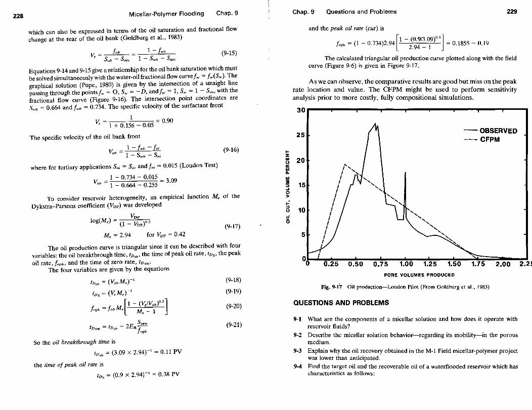
228 Micellar-Polymer Flooding Chap.9
which can also be expressed in terms of the oil saturation and fractional flow change at the rear of the oil bank (Goldburg eta!., 1983)
V,. = fob 1 - fwb Sob - Sore 1 - Swb - Sme
(9-15)
Equations 9-14 and 9-15 give a relationship for the oil bank saturation which must be solved simultaneously with the water-oil fractional flow curvefw = fw(Sw ). The graphical solution (Pope, 1980) is given by the intersection of a straight line passing through the pointsfw = 0, Sw = -D, andfw = 1, Sw = 1- Sore with the fractional flow curve (Figure 9-16). The intersection point coordinates are Swb = 0.664 and fwb = 0.734. The specific velocity of the surfactant front
1 v;. = 1 + 0.156- 0.05 = 0"
90
The specific velocity of the oil bank front
V, _ 1 - fwb - foi ob - 1 - Swb - Soi
where for tertiary applications So; = Sor and fo; = 0.015 (Loudon Test)
V, = 1 - 0.734- 0.015 = 3 09 ob 1 - 0.664 - 0.255 .
(9-16)
To consider reservoir heterogeneity, an empirical function M, of the Dykstra-Parsons coefficient (VDP) was developed
VoP log(M,) = (1 _ VDP)o 2
(9-17) M. = 2.94 for VoP = 0.42
The oil production curve is triangular since it can be described with four variables: the oil breakthrough time, tvob, the time of peak oil rate, tv,, the peak oil rate, fopk, and the time of zero rate, fvsw·
The four variables are given by the equations
tvob = (Vob M.)-1
tv,= (V,.M.)-1
~' = ~' M [1 - (V,.IVob)0
·5
] Jopk job e Me _ 1
So the oil breakthrough time is
tv.b = (3.09 X 2.94)-1 = 0.11 PV
the time of peak oil rate is
tv, = (0.9 X 2.94)-1 = 0.38 PV
(9-18)
(9-19)
(9-20)
(9-21)
1-z Ul u a: Ul IL
Ul ::& ::1 ..I 0 > ..: ::1 u ..I
0
Chap.9 Questions and Problems 229
and the peak oil rate (cut) is
[1 - (0 9/3 09)05
] fopk = (1 - 0.734)2.94
2_9
4 _·
1 = 0.1855- 0.19
The calculated triangular oil production curve plotted along with the field curve (Figure 9-6) is given in Figure 9-17.
As we can observe, the comparative results are good but miss on the peak rate location and value. The CFPM might be used to perform sensitivity analysis prior to more costly, fully compositional simulations.
30
25
20
15
10
5
00
,..., I ', I I I I I I I I I I I I I I I I
0.25 0.50 0.75 1.00 1.25
PORE VOLUMES PRODUCED
-OBSERVED --- CFPM
2.00 2.2f
Fig. 9-17 Oil production-Loudon Pilot (From Goldburg eta!., 1983)
QUESTIONS AND PROBLEMS
9-1 What are the components of a micellar solution and how does it operate with reservoir fluids?
9-2 Describe the micellar solution behavior-regarding its mobility-in the porous medium.
9-3 Explain why the oil recovery obtained in the M-1 Field micellar-polymer project was lower than anticipated.
9-4 Find the target oil and the recoverable oil of a waterflooded reservoir which has characteristics as follows:

230
Productive area
Net thickness
Porosity Irreducible water saturation
Formation volume factor for oil Initial Present
Oil recovery (present)
Capillary number
Oil saturation in
Micellar-Polymer Flooding
720 acres (2.9 x 10⁶ m2)
100 ft
26%
29%
1.26 1.15
46% 3 x 10⁻³
Waterflooded areas 25% Unswept regions 66%
Chap.9
9-5 Determine whether or not an MP system can be formulated for the reservoir whose characteristics are given in Example 9-1, assuming the residual oil saturation after waterflood is 31 percent, the oil saturation in unswept regions is 60 percent, and the oil viscosity in reservoir conditions is 2 cp.
9-6 Rework Example 9-2 using the same characteristic values.
REFERENCES
ATKINSON, H., U.S. Patent #1651311 (1927). BRAGG, J. R., W. W. GALE, JR., eta!., "EXXON Production Company: Loudon Sur
factant Flood Pilot Test," Society of Petroleum Engineers, SPE/DOE 10862 Paper, presented at the 1982 SPE/DOE Joint Symposium on Enhanced Oil Recovery, Tulsa, 0 klahoma, April 4-7, 1982.
COLE, L. E., "An Evaluation of the Robinson M-1 Commercial Scale Demonstration of Enhanced Oil Recovery by Micellar-Polymer Flood," Prepared by K&A Technology for the U.S. Department of Energy under Contract No. AC-19-85BC10830-10 (Bartlesville, OK: U.S. Department of Energy, December 1988).
DAUBEN, DWIGHT L., "A Review of the Loudon Surfactant Flood Pilot Test," work performed under contract No. AC-19-85BC10830-8 for U.S. Department of Energy (Bartlesville, OK: U.S. Department of Energy, November 1988).
DAVIS, J. A, and S. C. JONES, "Displacement Mechanisms of Micellar Solutions," Journal of Petroleum Technology (December 1969).
GOGARTY, W. B., "Miscible-Type Waterflooding: The Maraflood Oil Recovery Process," SPE of AIME: SPE 1847-A, 42nd Annual Fall Meeting, Houston, Texas,
October 1967. GoGARTY, W. B., and W. C. ToscH, "Miscible-Type Waterflooding: Oil Recovery with
Micellar Solution," Journal of Petroleum Technology (December 1968). GOLDBURG, A, H. PRICE, G. W. PAUL, and T. C. WESSON, "Selection of Reservoirs
Amenable to Micellar Flooding," Final Department of Energy Report, October 1978--December 1982, work performed by Department of Energy (U.S. DOE/ BC00048-29), August 1983.
Chap. 9 References 231
GUPTA, S. P., and S. TRUSHENSKI, "Micellar Flooding-Compositional Effects on Oil Displacement," Society of Petroleum Engineers Journal, Vol. 19 (1979), p. 116.
HEALY, R.N., R. L. REED, and C. W. CARPENTER, JR., "A Laboratory Study of Microemulsion Flooding," SPE Journal (February 1975).
HOLM,L. W., "Use of Soluble Oils for Oil Recovery," Journal of Petroleum Technology (December 1971).
HOLM, L. W., "Status of Micellar-Polymer Field Tests-Another View," Petroleum Engineering International (April 1980), pp. 100-16.
JONES, L. W., U.S. Patent #3126952 (March 31, 1964).
LAKE, LARRYW., Enhanced Oil Recovery (Englewood Cliffs, NJ: Prentice-Hall, 1989), Chapter 9.
LAKE, L. W., and G. A PoPE, "Status of Micellar-Polymer Field Test," Petroleum Engineering International (November 1979), pp. 38--60.
LATIL, M., Enhanced Oil Recovery (Paris: Edition Technip; distributed in United States by Gulf, Houston, TX, 1980), pp. 212-13.
LOWRY, P. H., H. H. FERRELL, and D. L. DAUBEN, "A Review and Statistical Analysis of Micellar-Polymer Field Test Data," Topical Report DOE/BC/10830-4 (Washington, D.C.: U.S. Department of Energy, November 1986).
PAUL, G. W., L. W. LAKE, and G. A POPE," A Simplified Predictive Model for MicellarPolymer Flooding," SPE 10733, presented at the 1982 California Regional Meeting ofthe Society of Petroleum Engineers, San Francisco, California, March 24-26, 1982.
POPE, G. A, "The Application,of Fractional Flow Theory to Enhanced Oil Recovery," SPE Journal (June 1980), pp. 191-205.
STOVER, D. F., "Commercial Scale Demonstration Enhanced Oil Recovery by MicellarPolymer Flood," Final Report, prepared by Marathon Oil Company for the U.S. Department of Energy under Contract No. AC-19-78ET13077 -130 (Bartlesville, 0 K: U.S. Department of Energy, November 1988).
TRUSHENSKI, S. P., D. L. DAUBEN, and D. R. PARRISH, "Micellar Flooding-Fluid Propagation, Interaction and Mobility," SPE Journal (December 1974).
U.S. DEPARTMENT OF ENERGY, "Selection of Reservoir Amenable to Micellar Flooding," First Annual Report DOE/BC/00048-20 (Bartlesville, OK: U.S. Department of Energy, December 1980).

Chapter 10
Carbon Dioxide Flooding
The use of carbon dioxide (C02) to increase the recovery of oil has received considerable attention since 1950. Laboratory research has been conducted and field applications have been initiated and performed indicating a great interest in C02 flooding.
To understand why C02 emerged as an important injection agent in oil reservoirs, we should note its principal properties and the factors that make it a useful tool in enhancing oil recovery.
10-1 PROPERTIES OF C02
Carbon dioxide is a colorless, odorless, inert, and noncombustible gas. It has a molecular weight of 44.01, which is one and a half times higher than that of air. The phase behavior of pure C02 is shown in Figure 10-1 on a P-T diagram.
C02 is solid at low temperatures and pressures. The solid carbon dioxide (dry ice) evaporates directly to gas at -78.SO C (-110.7° F) and is used primarily as a refrigerant. By increasing the pressure the liquid phase appears for the first time and coexists with the solid and vapor phases at the triple point:
232
I '
l l
Sec. 10-1
w 0:: ::::) (/) (/) w 0:: a..
Properties of C02
I
BOUNDARY ALONG WHICH SUPERCRITICAL PHASE TRANSITION IS ......... BELIEVED TO , ...... OCCUR ~ _,,'
~ ~ ,
~
, , ;'
;' ,
CRITICAL POINT
TRIPLE POINT
TEMPERATURE, °C
Fig. 10-1 Carbon dioxide phase diagram (From van Poollen, 1980)
233
triple point temperature I;, = -56.6° C ( -70.9° F), triple point pressure Ptr = 5.28 atm (77.6 psia). C02 is usually transported as a liquid in refrigerated trucks or tank cars when it can be utilized in small amounts. The liquid and the vapor phases of C02 coexist at the critical point: critical point temperature 1'c = ~0:1o C (87.8o F), critical point pressure Pc = 73 atm (1073 psia). Below the cnttcal temperature C02 can be either a liquid or a gas over a wide range of pressures. Above the critical temperature of 87.8° F, C02 (pure) will exist as a ga~ ~egardless of the pressure applied. However, at increasingly higher superc~tl~al pressures t~e vapor becomes and behaves more like a liquid. Most C02 p1pehnes ?perat.e m ~he supercritical range (van Poollen, 1980).
C02 density vanes Wtth pressure and temperature as does its viscosity and compressibility factor (Sage et al., 1955; Kennedy et al., 1961).
The density of '
C02 (solid) Ps = 1.512 g/cm3 (12.59 lb/gal) at triple point

234 Carbon Dioxide Flooding Chap. 10
C02 (liquid) p1 = 0.914 glcm3 at oo C (32° F) and 34.3 atm (504.2 psia)
C02 (gas) pg = 1.9768 giL (0.0164 lb/gal) at oo C and 1 atm (14.7 psia)
The specific gravity (relative density) of C02 (gas) d = 1.529 (air= 1) at oo C and 1 atm. Under many reservoir conditions the densities of C02 and oil are similar.
The viscosity of C02 is 0.0335 cp at the critical conditions of pressure and temperature, the critical compressibility factor is 0.275, and the specific heat (liquid) capacity at 300 psi is 0.5 Btu/lb-°F. The COz is more soluble in oil than in water (2 to 10 times more). Water also is soluble in C02 and must be removed by drying to prevent condensation and corrosion in the pipelines.
In- solution with water C02 increases water viscosity and forms carbonic acid, which has a beneficial effect on shaley rocks (reduction in pH stabilizes) and on calcareous rocks (dissolvin~ effect).
C02 is, from a chemical point of view, a final oxidation product of organic compounds with carbon, has acid character being the anhydrite of carbonic acid, and reacts with bases to form carbonates and bicarbonates. The principal C02 properties such as its acid function, its chemical inertia (protection gas, inert gas, pressure gas agent), its refrigerant function, and its high specific heat capacity explain the multiple utilization of C02 in different industries and processes.
C02 has many uses. It is frozen to produce dry ice, it is used to sterilize organic liquids, and it is used in cryogenics, foodstuffs manufacturing, refrigeration, and beverage carbonation. In the area of industry, C02 is used in heat transfer in nuclear reactors, in welding, in the manufacture of fertilizer and plastics, in neutralization of wastes, and in the manufacture of fire extinguishers. In medical and pharmaceutical applications it is found in salycilic acid for aspirin, mineral waters, and aerosol propellants, and it is used in cryogenic surgery. C02 is also used in pneumatic conveyor systems for coal and grain slurry lines, in the manufacture of white lead, for oil and gas stimulation, and for tank cleaning.
10-2 FACTORS THAT MAKE C02 AN EOR AGENT
Carbon dioxide is highly soluble in oil and to a lesser extent in water. This results in the following factors which contribute to enhanced oil recovery:
• Reduction in crude oil viscosity and increase in water viscosity • Swelling of crude oil and reduction in oil density • Acid effect on carbonate and shaley rocks • Miscibility effects
Oil viscosity is reduced significantly when C02 is dissolved in crude.
Sec. 10-2 Factors That Make C02 An EOR Agent
fLo= 1000 ~.~ r--.---.--.--r4~v:..;...r---.
51--+-~~1'--,t! 100
911------1
8H+----l
fLo 4 t-------+--+----++-/-+-V--1 fLm3 / "i 10 /v /~s
2 ~~~f-' I 0 200 400
1 HH+-----i SATURATION PRESSURE, PSIA
.6 Ht\t--+-----.-----.--.----.----1
fL m 5 J---tt-Hr+---+----t--+--+------4 J1. 0 . ~\
.I
.4 t-tt--H\\1-----+---~~ \t\
3r-1T~~-r-~--~-+---~
~-~~ ~ P-o \~~~ ~~~
r--:::::~ ~~~ t--~ -;,-'
L ____ JU·~~]~:::::±:==----~;,~soo~l_ __ _j 0 --- -1000
.2
0 1000 2000 ~
SATURATION PRESSURE. PSIA Fig. 10-2 Viscosity reduction versus saturation pressure (From Simon and Graue, 1965)
235
Figure 10-2 shows data from the work of Simon and Graue (1965). The symbol f.Lo refers to the original viscosity of the oil while f.Lm refers to the viscosity of that oil after saturation in C02 at equilibrium. The viscosity reduction, for e~am~le, is 10-fold at 2000 psia saturation pressure for an oil with original viscosity of 5 cp (5 mPa·s). This reduction in crude oil viscosity and an accompanying small increase in water viscosity reduces the water-oil mobility ratio.
Swelling of crude oil. As a result of C02 dissolved in the crude, the oil's v?lume ~ill increase from 10 to 20 percent or more. Figure 10-3 gives the crude ml swelhng factor (volume of COrsaturated crude at saturation pressure and
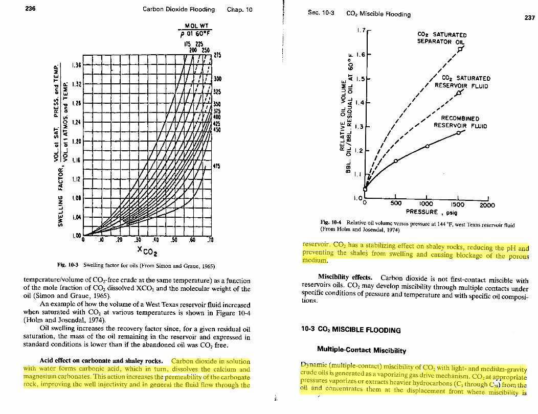
236
~ U6 ~ w t-
~ '0 c ~ 0 w
1.32
.n t-11'1 '0 w c
1.21 a: 0 Q. .n
0 ~ ~ 4 ~ 11'1
1.24
0 0 1.20
..J .J ~ 0
> 1.16 . a: 0 t-u 1.12 ~
"' z 1.0 I ~ ..J w ~ 11'1 ~
1.04
... ~ ~ 0 .. 10 1.00
Carbon Dioxide Flooding
I v I L
v '1.1. _j_ I Vi v i l_j
I v/ r.l. ~ 11'/.: ~ ~ ~ ~ V.I. ~ ~ ~
~ ~ ~ ~ ~ e:::: ~ ~ ~ p F'"""'
-.20 .30 .4 0
1 l1
1 VI lL r; [L '!J ~ t% ~ 1/
MOLWT pat so•F
J I v I
1/ I v,
i/ I
if} {h ~ VI v...,..
n~ m 200 250 Zl5
IJ I J !_1_
I J :
/ i/
I II 1/ I ""/
1/j VIJ VJ w ~ u. VI v '/ :z J v
v
_l_ 3
/3 00
25
~ TS 00 25 50
~·· ·' 3 3 '/i 4
W.t: !fjj 'J v J-
lJ 4 T5
.~0 .&0 .tO
Fig. 10-3 Swelling factor for oils (From Simon and Graue, 1965)
Chap. 10
temperature/volume of C02- free crude at the same temperature) as_a function of the mole fraction of C02 dissolved XC02 and the molecular wetght of the oil (Simon and Graue, 1965).
An example of how the volume of a West Texas reservoir fluid increased when saturated with C02 at various temperatures is shown in Figure 10-4 (Holm and Josendal, 1974). . . . .
Oil swelling increases the recovery factor smce, for. a gtven rest dual ~11 saturation, the mass of the oil remaining in the reservmr and expressed m standard conditions is lower than if the abandoned oil was C02 free.
Acid effect on carbonate and shaley rocks. Carbon dioxide in solution with water forms carbonic acid, which in turn, dissolves the calcium and magnesium carbonates. This action increases the permeabi~ity of the carbonate rock, improving the well injectivity and in general the flmd flow through the
Sec. 10-3 C02 Miscible Flooding
1.7
IL I. 6 0 0 ID
t-
w"' :I: .....I
3C5 ~...I
c(
:::!g oc;;
w ~a: 1.3 j::....J c(al ....Jal
""'' 0::51.2
....I m ml.l
COz SATURATED SEPARATOR OIL
/
/ /
/
p'
// C02 SATURATED / RESERVOIR FLUID
// /P' / ,
/ , / ,
/ ,.' / ,
I , I ,"'
I ' I // I /
I / ,I 1/
PRESSURE , psiQ
Fig. 10-4 Relative oil volume versus pressure at 144 °F, west Texas reservoir fluid (From Holm and Josendal, 1974)
237
reservoir. C02 has a stabilizing effect on shaley rocks, reducing the pH and preventing the shales from swelling and causing blockage of the porous medium.
Miscibility effects. Carbon dioxide is not first-contact miscible with reservoirs oils. C02 may develop miscibility through multiple contacts under specific conditions of pressure and temperature and with specific oil compositions:
10-3 C02 MISCIBLE FLOODING
Multiple-Contact Miscibility
Dynamic (multiple-contact) miscibility of C02 with light- and medium-gravity crude oils is generated as a vaporizing gas drive mechanism. C0
2 at appropriate
pressures vaporizes or extracts heavier hydrocarbons (C5 through C
30) from the
oil and concentrates them at the displacement front where miscibility is

238 Carbon Dioxide Flooding Chap. 10
100% C02
Fig. 10-5 Pseudoternary diagram vaporizing gas drive process with C02 (Adapted
from Stalkup, 1984)
achieved. Dynamic miscibility with C02 is possible through a vaporizing gas drive mechanism for reservoir fluid compositions lying to the right of the limiting tie line on a pseudoternary diagram (Figure 10-5).
The difference between the vaporizing gas drive mechanism with C02 and with natural gas (methane) is that dynamic miscibility with C02 does not require the presence of intermediate-molecular-weight hydrocarbons in the reservoir fluid. The extraction of a broad range of hydrocarbons from the reservoir oil often causes dynamic miscibility to occur at attainable pressures which are lower than the miscibility pressure for dry hydrocarbon gas (Stalkup, 1984).
Miscibility Pressure
The minimum miscibility pressure (MMP) above which dynamic miscible displacement with C02 is possible can be determined from displacement ~e~hniques and miscibility experiments. A review of methods for determmmg miscibility conditions is given by Stalkup (1984). The recommended methods for conducting and interpreting displacement techniques for determining miscibility conditions are gravity-stable experiments, slim tube experiments, and visual cell observations. Also, there have been several attempts to develop correlations from experimental studies of factors affecting C02 miscibility pressure.
Gravity-stable experiments use a vertically sandpacked and oil-saturated test column in which C02 injected at the top displaces the oil vertically downward at a rate slow enough to maintain a gravity-stable flow, overcoming the C0
2's tendency to protrude into the oil. The experiment is run at different
I.
Sec. 10-3
6'2.
i:":" "' :> 0 <.>
"' CI:
·-C)
C02 Miscible Flooding
100 90
80 70 60
50
40 30 20
10
0 1000
MMP '---!
2000 3000 4000 Pressure, Psig
5000
Fig. 10-6 The minimum miscibility pressure reached in a vertically test column
239
increasing pressures, and the ultimate oil recoveries (percentage of OOIP) obtained are plotted versus the respective pressures on the same graph (Figure 10-6). The minimum miscibility pressure is the pressure corresponding to the breakover point on the ultimate oil recovery curve.
Slim tube experiments are performed in a 40-ft-long, l-in.-diameter coiled stainless steel tube sandpacked and saturated with oil at a given pressure and temperature. The slim tube apparatus is provided with a capillary tube sight glass (Yelling and Metcalfe, 1980). The combination of small tube diameter, long tube length, and low flow velocity minimizes and suppresses C02 fingering. The results obtained for a series of C02 flood experiments in a slim tube apparatus are given in Figure 10-7. The plot of oil recovery versus pressure, after 1.2 PV of injection, shows a sharp break in the recovery curve, indicating the change from immiscible to miscible displacement as pressure is increased.
Visual cell observations can describe the gradual color change of the single-phase effluents as the transition zone changes from displaced oil to injected C02 • The interpretation of visual cell observations for C02 floods is not simple, requires an experienced observer, and may not describe all situations (Stalkup, 1984).
Correlations for estimating miscibility pressure have been made since reservoir temperature, oil composition, and characteristics are factors affecting this pressure. As stated by Stalkup (1984), there is a consensus that temperature is an extremely important parameter and that light ends in the oil (methane and nitrogen) and intermediate-molecular-weight hydrocarbons (ethane, propane and butane) have a small effect on C02 miscibility pressure.
Figure 10-8 shows the Holm and Josenthal correlation (1974) as extended by Mungan (1981). The oil composition, which is characterized by the molecular weight of the pentanes and heavier fractions, and reservoir temperature
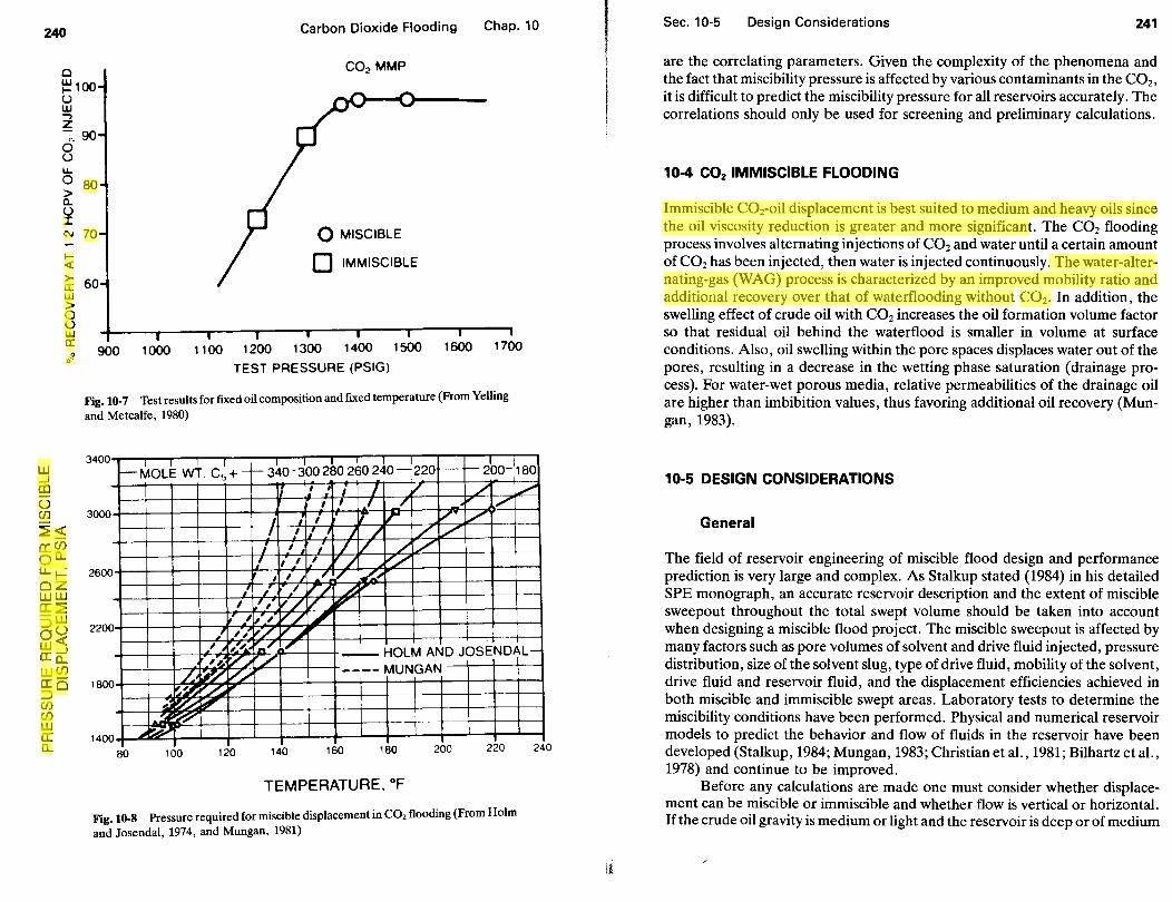
240 Carbon Dioxide Flooding Chap. 10
0 CO:>MMP
~100 u UJ .., z -;:, 90 0 u LL. 0 > a.. u I N
1-<{
>-a: UJ > 0 u UJ a: 0~
w ....J co (.) C/J ~<(
a:U5 oa.. u..-t-oz ww a:~ -w :::>(.) 0<( w_~
a: a.. wU)
a:cs :::> (/) (/) w a: Cl..
80
70 Q MISCIBLE
0 IMMISCIBLE
900 1000 1100 1200 1300 1400 1500 1600 1700
TEST PRESSURE (PSIG)
Fig. 10-7 Test results for fixed oil composition and fixed temperature (From Yelling and Metcalfe, 1980)
3400 f-~OL~ WT C~ +-1- 3~0- joo 2so 260 2Jo ~ 220 2b0-
1
180
I ,
I I I ,/ / / I _I .I _/ ./
3000 i i I IJ lr v v ! I 1/ ,I j / / ./
i I i I r/ / / 1.' I I I / V/
2600 1 I J ~/ fL; I
/ / ·' IT/ _AV I I 1.', ~-7 v " I[,'' '"/ ~
i ,, v/ v~ __(__ I , ....... r../ l/ - HOLM AND JOSENDAL-,,_ v .... /
---- MUNGAN ~· w V/ .~ ~ "" --!--
2200
1800
"~ ~ .:&! ~ --T ~
- I 0 140
80 100 120 140 160 180 200 220 240
TEMPERATURE, OF
Fig. 10-8 Pressure required for miscible displacement in C02 flooding (From Holm and Josendal, 1974, and Mungan, 1981)
il
Sec. 10-5 Design Considerations 241
are the correlating parameters. Given the complexity of the phenomena and the fact that miscibility pressure is affected by various contaminants in the C02 ,
it is difficult to predict the miscibility pressure for all reservoirs accurately. The correlations should only be used for screening and preliminary calculations .
10-4 C02 IMMISCIBLE FLOODING
Immiscible COToil displacement is best suited to medium and heavy oils since the oil viscosity reduction is greater and more significant. The C02 flooding process involves alternating injections of C02 and water until a certain amount of C02 has been injected, then water is injected continuously. The water-alternating-gas (WAG) process is characterized by an improved mobility ratio and additional recovery over that of waterflooding without C02 • In addition, the swelling effect of crude oil with C02 increases the oil formation volume factor so that residual oil behind the waterflood is smaller in volume at surface conditions. Also, oil swelling within the pore spaces displaces water out of the pores, resulting in a decrease in the wetting phase saturation (drainage process). For water-wet porous media, relative permeabilities of the drainage oil are higher than imbibition values, thus favoring additional oil recovery (Mongan, 1983).
10-5 DESIGN CONSIDERATIONS
General
The field of reservoir engineering of miscible flood design and performance prediction is very large and complex. As Stalkup stated (1984) in his detailed SPE monograph, an accurate reservoir description and the extent of miscible sweepout throughout the total swept volume should be taken into account when designing a miscible flood project. The miscible sweepout is affected by many factors such as pore volumes of solvent and drive fluid injected, pressure distribution, size of the solvent slug, type of drive fluid, mobility of the solvent, drive fluid and reservoir fluid, and the displacement efficiencies achieved in both miscible and immiscible swept areas. Laboratory tests to determine the miscibility conditions have been performed. Physical and numerical reservoir models to predict the behavior and flow of fluids in the reservoir have been developed (Stalkup, 1984; Mungan, 1983; Christian et al., 1981; Bilhartz et al., 1978) and continue to be improved.
Before any calculations are made one must consider whether displacement can be miscible or immiscible and whether flow is vertical or horizontal. If the crude oil gravity is medium or light and the reservoir is deep or of medium

242 Carbon Dioxide Flooding Chap. 10
depth, then miscible displacement should be considered. When the reservoir is of medium or shallow depth with medium or heavy gravity oil the miscibility pressure, if it exists, cannot be reached without surpassing the formation parting pressure. In this case displacement has to be immiscible but will include the beneficial effects of viscosity reduction and oil swelling.
The direction of displacement depends on reservoir geometry and characteristics. The horizontal displacement developed in nondip reservoirs with not so thick pay zone is controlled by the mobility ratio of C02 to oil. To avoid or diminish C02 fingering, the process should probably use alternating C02-
water injection. Vertical displacement is a characteristic of pinnacle reef or salt dome flank reservoirs and is controlled by the effect of gravity. To have a gravity-stable process, upward vertical displacement is achieved using water as a chasing fluid. Downward displacement is accomplished by using gas.
Flood Design and Performance Predictions
C02 flood design and performance predictions differ from reservoir to reservoir and for different operation strategies. However, there are features of C02
flooding that are more or less common to any field application. Examples of some of these features are presented in the paragraphs that follow.
Reservoir pressurization is an initial phase of the C02 miscible flood in which the reservoir pressure, reduced by primary depletion or some other recovery mechanism, has to be increased so that miscible displacement can occur. The reservoir pressure is usually increased by injecting water.
Example 10-1. Water is to be injected at an available rate of 12,580 bbllday (2000 m3/day) for reservoir pressurization. Although the original reservoir pressure of 2143 psi a was above the MMP of 2114 psi a, primary depletion had reduced the reservoir pressure to 1143 psia. The decision was made to return the reservoir to its original pressure before the start of C02 injection.
Calculate the total amount of injected water, W, and the time necessary for reservoir pressurization. The following data are known:
RESERVOIR DATA:
Oil formation volume factor
Gas formation volume factor
Solution ratio
Bo, = 1.53 at initial pressure Bo = 1.33 at actual pressure Bo, = 0.010 at initial pressure Bg = 0.014 at actual pressure R,, = 778 scf/bbl (137 m3/m3
) at initial pressure Rs = 522 scf/bbl (92 m3/m3) at actual pressure
Sec. 10-5 Design Considerations
PRODUCTION DATA: Cumulative oil produced Actual recovery factor Cumulative water produced Oil production rate (actual) Gas oil ratio
Water production rate (actual)
SOLUTION
243
Np = 2.516 X 10⁶ bbl (0.4 X 10⁶m3) ER = 15% of OOIP \¥p = 14 X 104 bbl (2.3 X 10⁴m3) qo = 1352 STB/day (215 m3/day) GOR (average) = 200 STB/bbl (m3fm3) qw = 126 bbllday (20 m3/day)
To pressurize the reservoir it is necessary to inject a total amount of water w that corresponds to the cumulative volume of fluids already produced Fp, plu~ th~ amount of fluids that will be produced during the pressurization phase, F;,P.
W = Fp + f;,p X pressurization time (10-1)
1. Calculate Fp. After 2.516 x 10⁶ bbl of oil has been produced the reservoir pore volume left free, Vg, is occupied by gas at actual reservoir pressure. Pressurization of these gases causes them to redissolve and occupy the volume v,,. Also considering the amount of water produced, Wp, we have
V, = NBo, - (N - Np)Bo
where N is the original oil in place
Vg,=V,X l Bg (R, - R,)!(Bo, - Bo)
and
2.516 X 10⁶ bbl V, =
0_15 X 1.53- (16.773- 2.516)
X 106 bbl X 1.33 = 6.7 X 10⁶ bbl
(10-2)
(10-3)
(10-4)
V: = 6. 7 X 106 bbl X 5.614 scf/bbl _ 6 gs 0.014 (778 - 522) scf!bbl/(1.53 - 1.33) - 2·1 X 10 bbl
Fp = 4.74 X 10⁶ bbl
2. Calculate F;,P. The reservoir volume of fluids produced daily, qr. is given by
(10-5)
where Bo, Bg, and l[. are the average formation volume factors and the average solution ratio, respectively.
Bo = 1.43, Bg = 0.011, and
between actual and pressurization pressure.

244 Carbon Dioxide Flooding
qf = 1352 X 1.43 + 1352(200- 5~~~4)0.011 + 126
= 3312 bbUday
Chap. 10
From the total daily amount of 12,580 bbl of water injected 3312 bbl are considered necessary to replace the fluids produced during pressurization.
3. Calculate the time necessary for pressurization.
Fp !pressurization = ---
q;- qf
where q; = 12,580 bbUday, the available rate of water injection
tpressurization = 511 days or 1.4 years
4. Calculate the total amount of water injected:
W = 4.74 x 10⁶ bbl + 3312 bbUday x 511 days
= 6.433 X 10⁶ bbl
(10-6)
Since the reservoir is produced under the dissolved gas drive mechanism, the water-injected downstructure (below the initial water-oil contact) will advance and displace the oil upward. The strategy of COz miscible displacement will have to be considered as a secondary operation in zones unswept or poorly swept by water and as a tertiary operation in the waterswept zones.
C02 requirements are determined in many ways depending on the reservoir geometry and displacement direction and on the miscibility conditions and injection strategy.
To illustrate one of the ways to estimate the volume of C02 needed for injection, the hypothetical simple example given by Mungan (1983) is given next.
Example 10-2. Estimate the total amount of COz needed for injection into a reservoir whose geometry (pinnacle reef) requires vertical, downward, and gravity-stabilized displacement and in which the COz is driven by nitrogen. The following data and information are known:
Pilot area Average thickness for oil zone
Average porosity Areal sweep efficiency
Vertical conformance Residual oil saturation in COrswept zone
Injection rate
A = 40 acres
h=300ft
<!> = 0.09
E.= 1.0 Ev = 0.8 Sor = 0.05 pore volume q; = 4000 bbUday
i:
Sec. 10-5 Design Considerations 245
It is assumed that at the time of COz breakthrough the C02 displacing bank appears as a mixing zone. The COz concentration decreases by diffusion from 90 percent in the middle of the bank to 10 percent at both the COz/oil downward and COz/nitrogen upward ends.
The length of the diffusion zone X is given (Perkins and Johnston, 1963) by
X = 3.625\.I'D.t (10-7)
where
t = the time that the COz front has been moving through the reservoir, seconds
D. = the effective diffusion coefficient, cm2/s
It is assumed that the diffusion coefficients for COz/oil and N2/C02 are on the same order as for hydrocarbon solvent floods and so
Dc-o = 3.5 X w-5 cm2/s
Dn.c = 65 X 10-5 cm2/s
SOLUTION
The volume of COz required is
(10-8)
where Vd is the amount corresponding to the mixing (diffusion) zone and v; is the amount that is soluble in the oil and water left behind the displacement front at floodout.
1. Calculate the amount of COz in the diffusion zone, Vd. The time required for the displacement front to reach the production wells is given (Mungan, 1983) by
f = (6.7 X 10⁸)Ah<j>E.Ev(1- So,) S
q; (10-9)
where the number 6. 7 x 10⁸ is the conversion constant for the units used
t = 6.7 X 10840 X 300 X 0.09 X 1 X 0.8(1 - 0.05) 4000
= 137.49 X 10⁶ S
The length of the diffusion (mixing) zone is written twice, once for C02/oil (c-o) and once for Nz/C02 (n-c ):
X90-w = 3.625(v'3.5 x 10⁻⁵ + V65 x 10-5)V137.49 x 106
= 1337 em= 43.9 ft
The C02 volume in the diffusion zone
Vd = A<!>X(7758) bbl 2 (10-10)

246 Carbon Dioxide Flooding Chap. 10
where the factor ! is used to integrate the concentration between the 10 and 90 percent values (Mungan, 1983)
Vd = 40 X 0.09 X 43.9(7758) = 613,037 bbl (97,473 m3) 2
or 7.37% pore volume
2. Calculate the amount of C02 dissolved behind the front, V.. The amount of C02 dissolved in the oil and water left behind the displacement front is calculated knowing the oil and water saturations in the swept and unswept zones the extent of the zones and the solubilities of COz in oil and water under the c~nditions of reservoir pressure and temperature, respectively.
Usually, when the residual oil saturation is low (efficient miscible displacement) an amount of 5 to 10 percent pore volume of COz is required to saturate the reservoir fluids. Assuming for our example that V. = 7.5% pore volume of C02 , the total volume of COz required is
Vco2 = 15% of pore volume
or
C02 injection pressure. When C02 is injected, care must be taken to ensure that the injection pressures are always below formation parting pressure. The surface C02 injection pressure value is calculated to assure the required miscibility pressure in the reservoir. The pressure exerted by the weight of the column of C02 gas at high pressure must be taken into consideration.
Example 10-3. Calculate the COz static wellhead pressure, P .. , when the static bottom hole pressure is the miscibility pressure of 2114 psia. The following additional information is available:
Bottom hole temperature
Surface temperature COz specific gravity
COz deviation factor
Reservoir depth
SOLUTION
TR = 170° F (76° C) T. = 70° F (21° C) SG = 1.529 (air = 1)
Z = 0.56 is assumed to be practically constant between reservoir pressure and temperature range
D = 4264 ft (1300 m)
The pressure exerted by the weight of a COz-gas column under ~atic conditions can be calculated by the average pressure and temperature method (Beggs, 1984). In conventional field units,
D = D [0.01875 SG(D)J rws rrs exp TZ (10-11)
Sec. 10-5 Design Considerations 247
where Pws is the static bottom hole pressure, psia, P15 is the static tubing pressure, psia, and Tis the average temperature in the tubing, 0R
2114 = P. ex [0.01875(1.529)(4264)] ts p 580(0.56)
and the COz static wellhead pressure is
2114 P .. = 1.45697 = 1451 psia
So the pressure exerted by the weight of a COrgas column under static conditions of p and Tis 663 psia.
Example 10-4. Calculate the tubing C02 injection pressure P,; when the injection bottom hole pressure Pw; is 2300 psia. The C02 injection rate averages q =:= 1 MM scf/day per injection well. Other data are
• Well tubing inside diameter, d = 2.441 in.
• The measured depth MD = TVD (true vertical depth) • The tubing roughness n = 5 X 10⁻⁴ in.
• The COz viscosity at 120° F and 2000 psia = 0.05 cp (from Stalkup, 1984). Other data are those given in Example 10-3.
SOLUTION The tubing COz injection pressure can be calculated using the same average pressure and temperature method (Beggs, 1984). The equation is
2 _ 2 (S) + 25(SG)q2
TZf(MD)[exp(S) - 1) (10
_12
) Pwt- Pt! exp Sds
where
Pwt = bottom flowing pressure (in this case, Pw;)
Ptf = tubing flowing pressure (in this case, Pn) S = 0.0375(SG)(TDV)/TZ
f = friction factor is given by
_1_ = 1.14 - 2 log(~ + 21.25) Vt d N:9 where the Reynolds number Ne is obtained from
N = pvg = 20,011(SG)q = 20,011(1.529) x 1 _ e j..L j..Ld 0.05(2.441) - 250,691
and
_1_ = 1 14- 2 lo (5 X 10⁻⁴ + 21.75 ) -Vt . g 2.441 (250,691)0·9 -8·516
f = 0.01379
s = 0.0375(1.529)(4264) -580(0.56) - 0·7527
(10-13)
248 Carbon Dioxide Flooding
exp(S) = exp(0.7527) = 2.1227
Now replacing in Eq. 10-12:
Chap. 10
2 25(1.529)12(580)0.56(0.01379)4264(2.1227- 1) (2300)
2 = Pn X 2.1227 + 0.7527(2.441)5
Pn = 1577 psia
The compressor horsepower required is that which is calculated to compress 1 MM scf/day of a 1.529-gravity gas (C02) from a given pressure and temperature to 1577 psia, plus the pressure drop in the well flow line and surface choke.
10-6 C02 DEMAND, SOURCES, AND TRANSPORTATION
C02 Demand
Carbon dioxide miscible displacement is one of the most promising EOR methods. Estimates of potential C02 demand in each of the four major U.S. basins studied in the DOE report (Anada et al., 1982) show the projected C02 requirement (based on 300 days injection per year) is as follows:
Permian Basin and Texas Gulf Coast= 10,011 MM scf/day Williston Basin 236 MM scf/day Appalachian Basin 83 MM scf/day Los Angeles Basin 376 MM scf/day
The DOE report also analyzed the injected C02 required per additional barrel of oil recovered. For example, in a secondary recovery process using C02, 13.5 M scf of C02 is needed to recover one additional barrel of light oil and 28.4 M scf of C02 is needed to recover one additional barrel of heavy oil. In a tertiary type of recovery using C02 (after waterflooding) 16.4 M scf of C02
is needed to recover one additional barrel of light oil. One can anticipate these figures being lowered to 6.8, 13.9, and 7.8 M scf/bbl, respectively, since over time a percentage of injected C02 is provided from a recycling process.
C02 Sources
A reliable source of supply for C02 is very important because the gas must be available on a continuous basis in large volumes for long periods of time, between 5 to 10 years or more. The C02 gas used must have a purity of 90 percent or more. If other gases such as methane or nitrogen are present with the C02 , a higher injection pressure is needed to render the gas miscible with the oil.
Sec. 10-7 Field Projects 249
The presence of HzS is undesirable because it is hazardous and detrimental to the environment. The presence of water vapor with the gas leads to corrosion so the C02 has to be dried.
The best C02 sources are naturally occurring high-pressure gas reservoirs with high-purity C02, mostly found while exploring for oil and gas. In the United States the oil producing basins of Wyoming, Utah, Colorado, and New Mexico have the largest COz reserves. The economics of a C02 miscible project are improved if C02 wells are located in the same geologic basins as those that produce oil, since the C02 transportation and injection pressure can then be partially supplied by the C02 reservoir pressure.
However, a DOE report (Anada et al., 1982) shows that currently known naturally occurring high-purity C02 sources can only provide less than 15 percent of the total C02 demand. Other natural C02 sources are natural gas fields containing C02 which is removed in gas processing plants (Delaware and Val Verde basins of Southwest Texas). These, along with any sources which incidentally produced C02 as a by-product, are more than sufficient to satisfy the C02 demand. The sources which produce C02 as an offgas are coal-, oil-, and gas-fired power plants (which generate large quantities of flue gas containing C02), cement and ammonia plants, refineries, and ethanol and ethylene oxide plants, among others.
The most convenient C02 source must be considered for each particular process application, and favorable circumstances must be exploited in time to reduce the technology cost for extraction of C02 and the cost of compression, transportation, and injection.
Transportation of C02
The method of transportation of C02 from its source to the oil field depends on whether the C02 is liquid or gas. For small injection rates of 1 to 5 MM scf/day and short injection periods, C02 is liquefied at its source and transported to the project sites by refrigerated trucks, tank trucks, tank cars on rail or in storage tanks located on barges. Transporting the C02 liquid at oo F and 300 psi using existing insulated steel containers is the least costly method of transportation (Anada et al., 1982). The C02 necessary for large long-term projects is transported most economically through a pipeline as vapor at pressures between 1400 to 2000 psi (which are above the critical pressure) so that two-phase flow does not occur.
10-7 FIELD PROJECTS
~ince th~ early ~9?0s _when higher oil prices began to generate widespread mterest m C02 mJectwn, numerous articles have been written about field
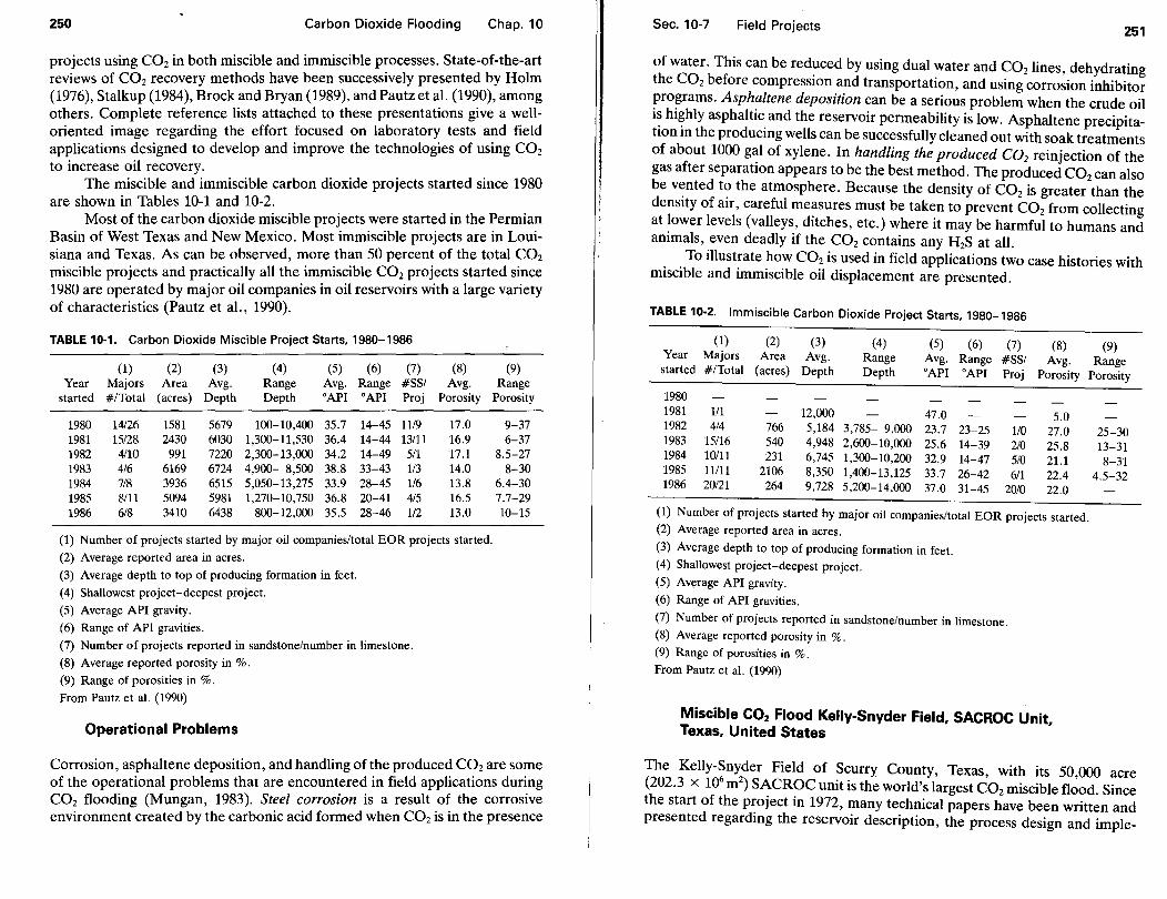
250 Carbon Dioxide Flooding Chap. 10
projects using C02 in both miscible and immiscible processes. State-of-the-art reviews of C02 recovery methods have been successively presented by Holm (1976), Stalkup (1984), Brock and Bryan (1989), and Pautz et al. (1990), among others. Complete reference lists attached to these presentations give a welloriented image regarding the effort focused on laboratory tests and field applications designed to develop and improve the technologies of using COz to increase oil recovery.
The miscible and immiscible carbon dioxide projects started since 1980 are shown in Tables 10-1 and 10-2.
Most of the carbon dioxide miscible projects were started in the Permian Basin of West Texas and New Mexico. Most immiscible projects are in Louisiana and Texas. As can be observed, more than 50 percent of the total COz miscible projects and practically all the immiscible C02 projects started since 1980 are operated by major oil companies in oil reservoirs with a large variety of characteristics (Pautz et al., 1990).
TABLE 10-1. Carbon Dioxide Miscible Project Starts, 1980-1986
(1) (2) (3) (4) (5) (6) (7) (8) Year Majors Area Avg. Range Avg. Range #SS/ Avg.
started #/Total (acres) Depth Depth 0 API 0 API Proj Porosity
1980 14/26 1581 5679 100-10,400 35.7 14-45 1119 17.0 1981 15/28 2430 6030 1 ,300-11 ,530 36.4 14-44 13/11 16.9 1982 4/10 991 7220 2,300-13,000 34.2 14-49 5/1 17.1 1983 4/6 6169 6724 4,900- 8,500 38.8 33-43 113 14.0 1984 7/8 3936 6515 5,050-13,275 33.9 28-45 116 13.8 1985 8/11 5094 5981 1,270-10,750 36.8 20-41 4/5 16.5 1986 6/8 3410 6438 800-12,000 35.5 28-46 112 13.0
(1) Number of projects started by major oil companies/total EOR projects started.
(2) Average reported area in acres.
(3) Average depth to top of producing formation in feet.
( 4) Shallowest project-deepest project.
(5) Average API gravity.
(6) Range of API gravities.
(7) Number of projects reported in sandstone/number in limestone.
(8) Average reported porosity in %.
(9) Range of porosities in %.
From Pautz et al. (1990)
Operational Problems
(9) Range
Porosity
9-37 6-37
8.5-27 8-30
6.4-30 7.7-29 10-15
Corrosion, asphaltene deposition, and handling of the produced C02 are some of the operational problems that are encountered in field applications during C02 flooding (Mungan, 1983). Steel corrosion is a result of the corrosive environment created by the carbonic acid formed when C02 is in the presence
Sec. 10-7 Field Projects 251
of water. This can be reduced by using dual water and C02 lines, dehydrating the COz before compression and transportation, and using corrosion inhibitor programs. Asphaltene deposition can be a serious problem when the crude oil is highly asphaltic and the reservoir permeability is low. Asphaltene precipitation in the producing wells can be successfully cleaned out with soak treatments of about 1000 gal of xylene. In handling the produced C02 reinjection of the gas after separation appears to be the best method. The produced C02 can also be vented to the atmosphere. Because the density of C02 is greater than the density of air, careful measures must be taken to prevent C02 from collecting at lower levels (valleys, ditches, etc.) where it may be harmful to humans and animals, even deadly if the C02 contains any H2S at all.
To illustrate how C02 is used in field applications two case histories with miscible and immiscible oil displacement are presented.
TABLE 10-2. Immiscible Carbon Dioxide Project Starts, 1980-1986
(1) (2) (3) (4) (5) (6) (7) (8) (9) Year Majors Area Avg. Range Avg. Range #SS/ Avg. Range started #/Total (acres) Depth Depth 0 API 0 API Proj Porosity Porosity
1980 1981 111 12,000 47.0 5.0 1982 4/4 766 5,184 3,785- 9,000 23.7 23-25 110 27.0 1983 15/16 540 4,948 2,600-10,000 25.6 14-39 210 25.8 1984 10/11 231 6,745 1 ,300-10,200 32.9 14-47 510 21.1 1985 11/11 2106 8,350 1 ,400-13,125 33.7 26-42 6/1 22.4 1986 20/21 264 9,728 5,200-14,000 37.0 31-45 20/0 22.0
(1) Number of projects started by major oil companies/total EOR projects started. (2) Average reported area in acres.
(3) Average depth to top of producing formation in feet. (4) Shallowest project-deepest project. (5) Average API gravity.
(6) Range of API gravities.
(7) Number of projects reported in sandstone/number in limestone. (8) Average reported porosity in%. (9) Range of porosities in %.
From Pautz et al. (1990)
Miscible COz Flood Kelly-Snyder Field, SACROC Unit, Texas, United States
25-30 13-31 8-31
4.5-32
The Kelly-Snyder Field of Scurry County, Texas, with its 50,000 acre (202.3 x 10
6m
2) SACROC unit is the world's largest C02 miscible flood. Since
the start of the project in 1972, many technical papers have been written and presented regarding the reservoir description, the process design and imple-
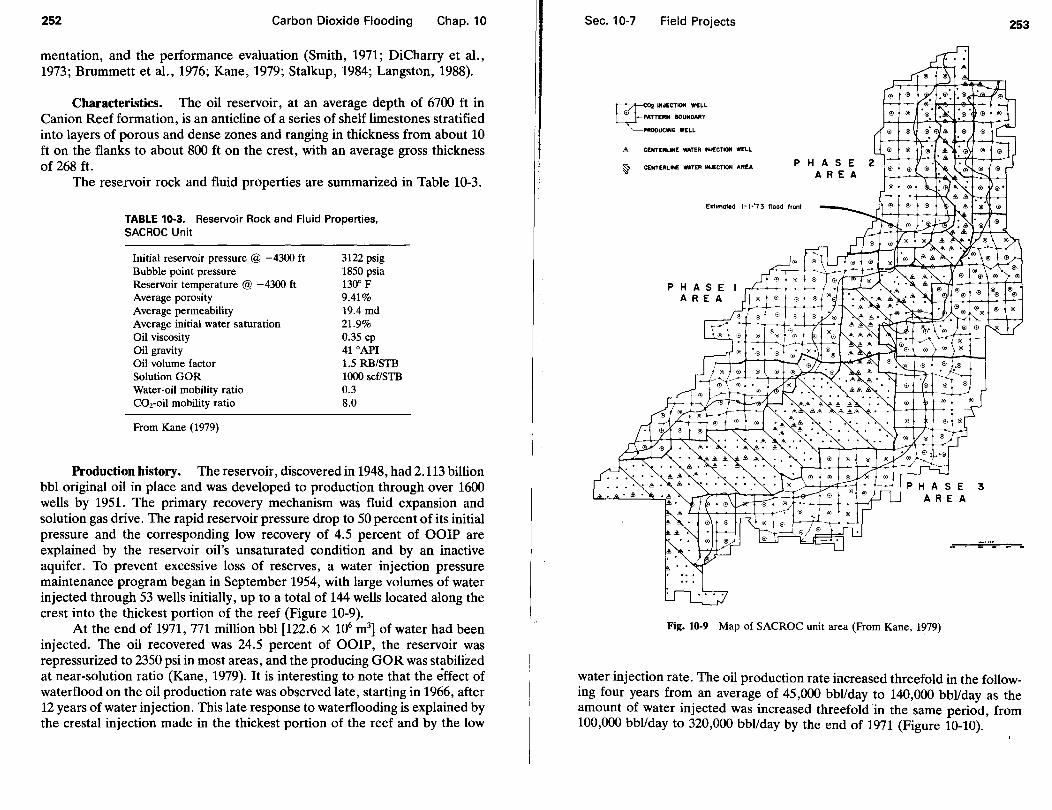
252 Carbon Dioxide Flooding Chap. 10
mentation, and the performance evaluation (Smith, 1971; DiCharry et al., 1973; Brummett et al., 1976; Kane, 1979; Stalkup, 1984; Langston, 1988).
Characteristics. The oil reservoir, at an average depth of 6700 ft in Canion Reef formation, is an anticline of a series of shelf limestones stratified into layers of porous and dense zones and ranging in thickness from about 10 ft on the flanks to about 800 ft on the crest, with an average gross thickness of 268ft.
The reservoir rock and fluid properties are summarized in Table 10-3.
TABLE 10-3. Reservoir Rock and Fluid Properties, SACROC Unit
Initial reservoir pressure @ -4300 ft Bubble point pressure Reservoir temperature @ -4300 ft Average porosity Average permeability Average initial water saturation Oil viscosity Oil gravity Oil volume factor Solution GOR Water-oil mobility ratio CO,-oil mobility ratio
From Kane (1979)
3122 psig 1850 psia 130" F 9.41% 19.4 md 21.9% 0.35 cp 41 °API 1.5 RB/STB 1000 scf/STB 0.3 8.0
Production history. The reservoir, discovered in 1948, had 2.113 billion bbl original oil in place and was developed to production through over 1600 wells by 1951. The primary recovery mechanism was fluid expansion and solution gas drive. The rapid reservoir pressure drop to SO percent of its initial pressure and the corresponding low recovery of 4.5 percent of OOIP are explained by the reservoir oil's unsaturated condition and by an inactive aquifer. To prevent excessive loss of reserves, a water injection pressure maintenance program began in September 1954, with large volumes of water injected through 53 wells initially, up to a total of 144 wells located along the crest into the thickest portion of the reef (Figure 10-9).
At the end of 1971, 771 million bbl [122.6 x 10⁶ m3] of water had been
injected. The oil recovered was 24.5 percent of OOIP, the reservoir was repressurized to 2350 psi in most areas, and the producing GOR was stabilized at near-solution ratio (Kane, 1979). It is interesting to note that the effect of waterflood on the oil production rate was observed late, starting in 1966, after 12 years of water injection. This late response to waterflooding is explained by the crestal injection made in the thickest portion of the reef and by the low
Sec. 10-7 Field Projects
COt; INJECTION WELL
PATTE:RN BOUNDARY
PRODUCING WELL
~ CENTERLINE WATER INJECTtoN WELL
~ CENTERLINE: WATER WJECTION AREA P H A S E ARE A
Estimated 1-1·'73 flood front
P H AS E AREA
Fig. 10-9 Map of SACROC unit area (From Kane, 1979)
253
3
water injection rate. The oil production rate increased threefold in the following four years from an average of 45,000 bbl/day to 140,000 bbl/day as the amount of water injected was increased threefold 'in the same period, from 100,000 bbl/day to 320,000 bbl/day by the end of 1971 (Figure 10-10).

254 Carbon Dioxide Flooding Chap. 10
! l ~ .. v :~r.ar- --- -~ --r- r--r- -J?- ~1---1~-t-+-+--+--+--r--t--t---t---l ~ - .... -+- -. -- i' - t--r-1 /~. / lz_
- - ~ i . +--~~~::+-+-+-t----t--t--t-+--t---t--+-+---i ! ~ ~p
; :
!
;;
.. --
- ---
• ~ : I I i i 1 i i i ; i 'i i I ~ i I i I i • • ! .. _,_I....,.Ct~llnt:-•--w-..s:IIOioi I! iII I IiI J I J
Cot _,_Mtl-f_,.._OI'".rll'lll-'f ........ Mnt-CV.n 'Itt-
Fig. 10-10 Kelly-Snyder Field performance summary (From Kane, 1979)
Sec. 10-7 Field Projects 255
COz·WAG Project
Since the center-line injection system was considered incapable of supporting production on the flanks of the reef (Langston et al., 1988), the feasibility of modifying or replacing the center-line system was investigated, and an inverted 9-spot injection pattern flooding with C02 in a WAG as a secondary process was considered to be the most efficient alternative (Hull, 1970). Since the delivery rate of 200 MMcf/day [5.66 X 10⁶ m3/d] of C02 was about one-third the total pattern area injection requirement, the C02 pattern injection scheme was implemented by developing the field area in three "phases" of similar hydrocarbon pore volume (Figure 10-9), which were to be flooded sequentially. To assure that the minimum miscibility pressures of about 2300 psia were attained, pre-C02 water slugs of 6 percent HCPV were injected in low-pressure patterns, followed by COr WAG cycles. The WAG-cycle slug volumes were 6 percent HCPV C02 followed by 2.8 to 3.6 percent HCPV water for an average WAG ratio of 0.55: 1.
The C02 obtained as by-product at several gas plants was delivered to the site through 220 miles of pipeline in supercritical condition provided by four compressor and two booster stations. Dual water and C02 injection lines were installed to the COr WAG injection wells. The water was injected at 2000 psi by four high-pressure water injection stations using centrifugal pumps. The C02 compressor discharge pressure ranges from 2200 to 2400 psig. Mter separation, the produced gas was processed at three gasoline plants using hot potassium carbonate and amine C02 removal systems with a total C02 removal capacity of 56 MMcf/day (1.59 x 10⁶ m3/d). The C02-WAG injection process started in January 1972 in the phase 1 area, and the cumulatives and rates through December 1977 are summarized in Table 10-4 (Kane, 1979).
TABLE 10-4. Injection Status in Nine-Spot Pattern Areas C02-WAG Project, SACROC Unit
Phase Phase 1 2
C02-WAG injection began I, 1972 III, 1974
Cumulatives, through December 1977 C02, BSCF 184 142 C02,% HCPV 14.3 10.0 Water, million bbl 290 200 Water, % HCPV 49.9 30.3
Rates, as of December 1977 C02 MM scf/day 20 93 Water, million bbl 189 150
From Kane (1979)
Phase 3
XI, 1976 Total
18 344 1.4 av 8.6
193 683 31.2 av 37.1
34 147 141 480
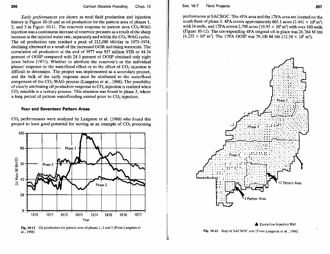
256 Carbon Dioxide Flooding Chap. 10
Early performances are shown as total field production and injection history in Figure 10-10 and as oil production for the pattern area of phases 1, 2, and 3 in Figure 10-11. The reservoir response to pattern area C02-WAG injection was a continuous increase of reservoir pressure as a result of the sharp increase in the injected water rate, separately and within the C02-WAG cycles. The oil production rate reached a peak of 212,000 bbl/day in 1973-1974, declining afterward as a result of the increased GOR and rising watercuts. The cumulative oil production at the end of 1977 was 937 million STB or 44.34 percent of OOIP compared with 24.5 percent of OOIP obtained only eight years before (1971). Whether to attribute the reservoir's or the individual phases' response to the waterflood effect or to the effect of C02 injection is difficult to determine. The project was implemented as a secondary project, and the bulk of the early response must be attributed to the waterflood component of the COr WAG process (Langston et al., 1988). The possibility of clearly attributing oil production response to C02 injection is realized when C02 miscible is a tertiary process. This situation was found in phase 3, where a long period of pattern waterflooding existed prior to C02 injection.
Four and Seventeen Pattern Areas
C02 performances were analyzed by Langston et al. (1988) who found this project to have good potential for serving as an example of C02 processing
1972 1973 1974 1975 1976 Year
Fig. 10-11 Oil production for pattern area of phases 1, 2 and 3 (From Langston et al., 1988)
Sec. 10-7 Field Projects 257
performance at SACROC. The 4PA area and the 17PA area are located on the south flank of phase 3. 4PA covers approximately 603.1 acres (2.441 x 10⁶m2)
with 24 wells, and 17PA covers 2,700 acres (10.93 x 1()6 m2) with over 100 wells (Figure 10-12). The corresponding 4PA original oil in place was 26,764 M bbl (4.255 x 10⁶ m3
). The 17PA OOIP was 79,100 M bbl (12.58 x 10⁶ m3).
. :' ::-: ~:.: ::::.:: ::)/.:..~ :: ; :'.: ~ :.::·~·::·:~·-..:·:. : ........ : .. : ...... ; ; ; · ... ::: : . . . . . . . . . .
• · • .. ·. Phase 3 • : •• •. • • • • • !'. • · . · · . ·: · · · · : : ... : ·. ; : ·. : ·. : ~: ~: . ~-:: .. : : •.· ......... : : ~: . : ~ .: ·. ~
••• 0 ••• ~ • ••• : ••• : 0
. . . . . . . . . . . . . . . . . .. : ...... · ......... ~ ~-· . . . . . . . . . . . . . . . . . . .· .... . • • • • 0 • 0 • • • • • • • • • • • • : •••••• . . . . . . . . . . : ..... : . . . ...... .
L.o..o......:....a..:.· .:..• -;· • . . . . . . . . ..
A Centerline Injection Well
Fig. 10-12 Map of SACROC unit (From Langston et al., 1988)

258 Carbon Dioxide Flooding Chap. 10
Before the start of the C02-WAG process in May-June 1981, the 4PA area was placed on a pattern waterflood in April1973 and the 17PA area was influenced by center-line secondary recovery injection. Cumulative C02 injection as of December 1987 represented 29.2 percent of the 4PA hydrocarbon pore volume and 17.5 percent of the 17PA HCPV. The performances of both pattern areas are shown in Figures 10-13 and 10-14. The "factored production" refers to production allocated to a pattern from a pattern side well or from a well located on a pattern corner (Langston et al., 1988).
The decline curve analysis from which a production decline rate was determined starting with the pre-C02 injection period and extrapolated into the future shows the quantitative response to C02 injection as follows:
The incremental oil production in the 4PA as result of the C02 miscible process is estimated to be 10.2 percent of OOIP and 7.5 percent of OOIP in the 17P A. The ratio of cumulative C02 injection to cumulative incremental oil production, which is the cumulative utilization of the injected C02, is about 9600 fe/bbl (1718 m3/m3
).
The ultimate recovery fieldwide can be estimated as being 19 percent of OOIP in primary as studies indicated, plus about 22 percent in secondary as result of waterflood, plus at least 9 percent in tertiary with the C02 miscible process, for a total of 50 percent of OOIP.
The performance of the large-scale C02-WAG project conducted at the SACROC Unit-Kelly-Snyder Field showed that effective C02 miscible processes can be developed and implemented to recover additional residual crude oil using large volumes of C02 transported long distances, distributed to injectors, and injected successfully.
Immiscible C02 Project, Tar Zone, Wilmington Field, California, United States
This project is an example of the use of C02 for immiscible flooding in heavy oils. The presentation and the data that follow are summarized from the article review written by Spivak et al. (1990).
Characteristics. The oil reservoir-the Tar Zone-is the uppermost producing zone in the Fault Block V of the Wilmington anticline structure and includes subzones S, T, and F, which consist of a series of loosely consolidated sands with an average gross thickness of 300 ft. The reservoir rock and fluid characteristics are given in Table 10-5.
Production history. The original oil in place in the project area was 69.465 x 10⁶ STB (11.045 x 10⁶ m3
). The total oil produced, from 1961 under waterflood, was 23.27 percent of OOIP up to 95 percent watercut. In March 1982, an immiscible C02 displacement was started as a tertiary recovery mechanism.
Sec. 10-7 Field Projects 259
40,000 .--------------~i'-iij-r--------.
10,000
1,000
Water Production (Bbi/D) _ • .a.~ 1\ •• u-T- 1 .. ... ~ .......... .__ ..... ,.; ... ,_,.. , ..
Projected Base Oil Rate
C02 Injection Begins June 1981
~(Bbi/D)
~~~ ~
77 78 79 80 81 82 83 84 Year
85
~ '---···.:
C02 Production (Mft 3/D)
\ 86 87 88
Fig. 10-13 Four pattern area performance summary (From Langston eta!., 1988)
100,000-r---------------------...,
10,000
1,000
.. _._ ......... ..,.,..., ....~· • .r
Water Production (Bbi/D) / ... ... , ,..-,. ........... _.~ ..
77 78 79 80 81 82 83 84 85 86 87 88
Year
Fig. 10-14 Seventeen pattern area performance summary (From Langston et al., ' 1988)

260 Carbon Dioxide Flooding
TABLE 10-5. Reservoir Rock and Fluid Properties Tar Zone, Wilmington Field, California
Project surface area Depth Initial pressure Reservoir temperature Reservoir dip Average net oil pay Porosity Permeability Permeability Permeability Initial oil saturation Oil gravity Oil viscosity (res. cond.) Initial solution GOR Oil volume factor
330 acres 2300 ft 1000 psig 120° F 9.5° to the south* 141 ft 27% 100 md (S) 500 md (T) 400 md (F) 75% 14 °API 180 to 410 cp 87 scUSTB 1.05
• In the southern portion of the project area.
From Spivak et a!. (1990)
Chap. 10
The C02 injection was begun downstructure and half central as a WAG process (Figure 10-15).
Water and C02 were injected on a two-week cycle schedule. The gas-towater ratio was reduced after an early breakthrough to the order of 1.0 on a reservoir-volume basis, to control the adverse mobility ratio. After the alternate injection of 12 percent HCPV C02, water was injected continuously to displace the less viscous oil (with C02 in solution). The improved relative permeability conditions and the oil swelling in addition to the viscosity reduction were the beneficial effects of the C02-WAG process.
The injected gas was an 85 percent C02 and 15 percent Nz mixture provided as stack gas from hydrogen generation units in the area. The total amount of 8.22 billion scf (230 x 106 m3
) of gas C02 was purchased and injected as of July 1986 when gas injection was terminated. This amount represents only 30 percent of the theoretical maximum gas requirements ( 40 percent of HCPV). Water injection rates averaged about 20,000 STB/day (3180 m3/d) since 1984.
The theoretical calculation of the incremental oil recovery achieved by the immiscible C02 process was made using the Buckley-Leverett-type two-phase immiscible analysis. The technique was to compare the oil recovery through continued waterflooding with the oil recovery obtained using the modified flow properties expected from immiscible C02 flood. The water-oil mobility ratio is improved when the oil viscosity at maximum oil saturation is reduced from about 406 cp to 54 cp. The results showed that cumulative recovery at watercut 95 percent (WOR = 20) was 21.9 percent of OOIP for the continued waterflood compared with 31.7 percent of OOIP for the immiscible C02 process or 6.66 x 10⁶ STB [1.06 x 10⁶ m3
] additional oil over a 20-year period. By inject-
Sec. 10-7 Field Projects
" CO:t WAG INJECTO~ }1 WATER INJECTOR
0 PRQQUCER
\ -... , ........
Fig. 10-15 Subzone F1 scaled-down area (From Spivak eta!., 1990)
261
ing less C02 than required to saturate all the oil fully, the oil viscosity would be proportionally higher and the recovery lower. Figure 10-16 shows the oil rate and the gas production rate for the period from March 1982.
Performance evaluation. As can be observed from Figure 10-16, gas breakthrough occurred after about one year of C02 injection and the gas production increased significantly.
Because of downstructure injection the gravity override effect that causes gas to migrate updip was probably greater in Subzone S, a massive clean sand with high permeability. To reduce this effect the gas-to-water ratio of 1.23 M scf/STB (222 m3/m3
) was changed to less than 1.0 on a reservoir-volume basis and WAG cycles were reduced to about 2 weeks. As can be observed, gas production was brought under control in late 1983. The oil rate performance shows dependence on gas injection as the driving agent, as the oil rate increased sharply at the beginning of 1985 when injection was concentrated in the scaled-down area (Figure 10-15) and then dropped soon after curtailment of C02 purchases in the spring of 1986. Incremental tertiary oil recovery as of the end of August 1987 was 488,000 STB (77 ,590 m3) and is most probably the oil
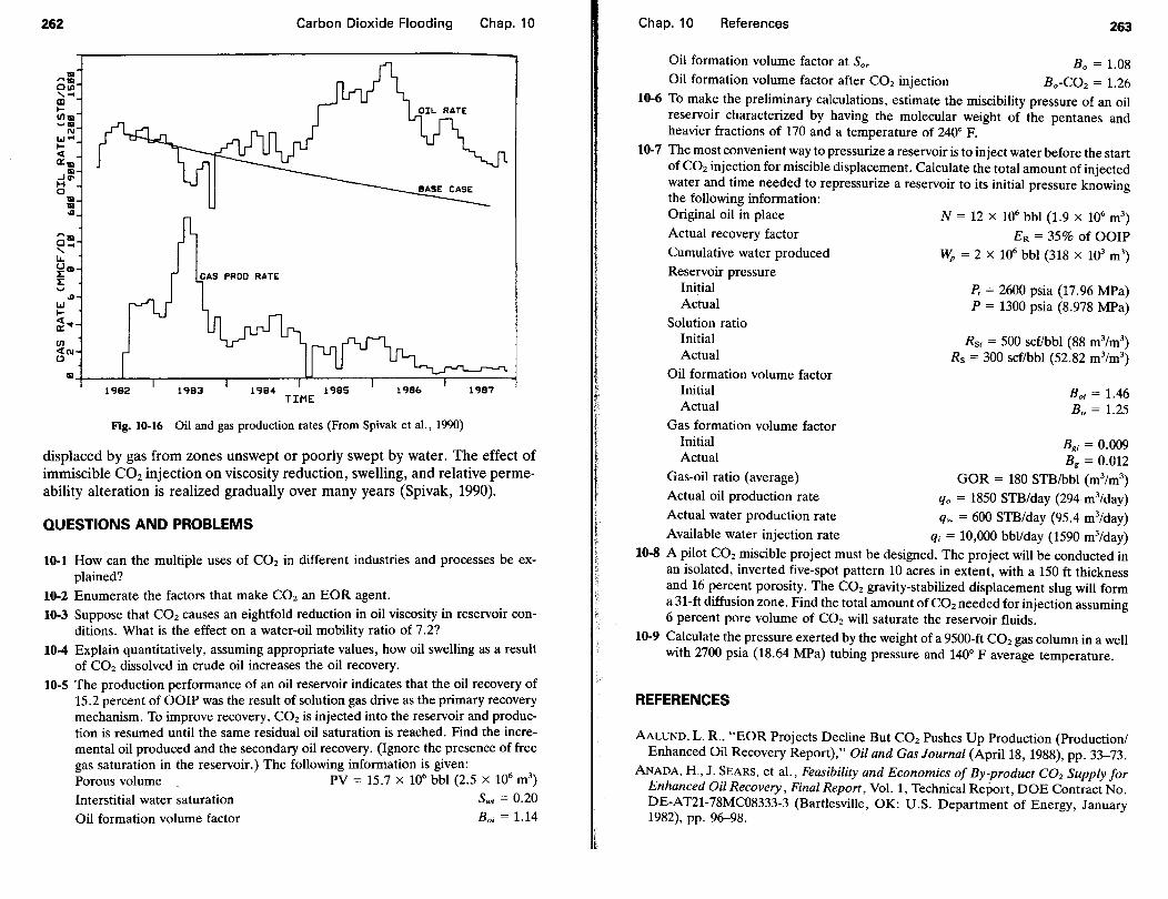
262
111 ..... 01.11 , .. CD 1-(/)111 .....
N w .. 1-.q cr • ...Jg! H 0
111 111 .a
Carbon Dioxide Flooding Chap. 10
Fig. 10-16 Oil and gas production rates (From Spivak eta!., 1990)
displaced by gas from zones unswept or poorly swept by water. The effect of immiscible C02 injection on viscosity reduction, swelling, and relative perme· ability alteration is realized gradually over many years (Spivak, 1990).
QUESTIONS AND PROBLEMS
10-1 How can the multiple uses of C02 in different industries and processes be explained?
10-2 Enumerate the factors that make COz an EOR agent. 10-3 Suppose that C02 causes an eightfold reduction in oil viscosity in reservoir con
ditions. What is the effect on a water-oil mobility ratio of 7.2? 10-4 Explain quantitatively, assuming appropriate values, how oil swelling as a result
of C02 dissolved in crude oil increases the oil recovery. 10-5 The production performance of an oil reservoir indicates that the oil recovery of
15.2 percent of OOIP was the result of solution gas drive as the primary recovery mechanism. To improve recovery, COz is injected into the reservoir and production is resumed until the same residual oil saturation is reached. Find the incremental oil produced and the secondary oil recovery. (Ignore the presence of free gas saturation in the reservoir.) The following information is given: Porous volume . PV = 15.7 x 10⁶ bbl (2.5 x 10⁶ m3
)
Interstitial water saturation Swt = 0.20 Oil formation volume factor Boi = 1.14
Chap. 10 References 263
Oil formation volume factor at Sor
Oil formation volume factor after COz injection Bo = 1.08
Ba·COz = 1.26 10-6 To make the preliminary calculations, estimate the miscibility pressure of an oil
reservoir characterized by having the molecular weight of the pentanes and heavier fractions of 170 and a temperature of 240° F.
10-7 The most convenient way to pressurize a reservoir is to inject water before the start of C02 injection for miscible displacement. Calculate the total amount of injected water and time needed to repressurize a reservoir to its initial pressure knowing the following information: Original oil in place Actual recovery factor Cumulative water produced Reservoir pressure
Initial Actual
Solution ratio Initial Actual
Oil formation volume factor Initial Actual
Gas formation volume factor
N = 12 X 106 bbl (1.9 X 10⁶ m3)
ER = 35% of OOIP Wp = 2 X 10⁶ bbl (318 X 103 m3
)
P; = 2600 psia (17.96 MPa) P = 1300 psia (8.978 MPa)
Rst = 500 scf/bbl (88 m3/m3)
Rs = 300 scflbbl (52.82 m3/m3)
Boi = 1.46 Bo = 1.25
Initial Bg1 = 0.009 Actual Bg = 0.012
Gas-oil ratio (average) GOR = 180 STB/bbl (m3/m3)
Actual oil production rate qo = 1850 STB/day (294m3/day) Actual water production rate qw = 600 STB/day (95.4 m3/day) Available water injection rate q1 = 10,000 bbUday (1590 m3/day)
10-8 A pilot COz miscible project must be designed. The project will be conducted in an isolated, inverted five-spot pattern 10 acres in extent, with a 150 ft thickness and 16 percent porosity. The C02 gravity-stabilized displacement slug will form a 31-ft diffusion zone. Find the total amount of COz needed for injection assuming 6 percent pore volume of COz will saturate the reservoir fluids.
10-9 Calculate the pressure exerted by the weight of a 9500-ft COz gas column in a well with 2700 psia (18.64 MPa) tubing pressure and 140° F average temperature.
REFERENCES
AALUND, L. R., "EOR Projects Decline But COz Pushes Up Production (Production/ Enhanced Oil Recovery Report)," Oil and Gas Journal (April18, 1988), pp. 33--73.
AN ADA, H., J. SEARS, et a!., Feasibility and Economics of By-product C02 Supply for Enhanced Oil Recovery, Final Report, Vol. 1, Technical Report, DOE Contract No. DE-AT21-78MC08333-3 (Bartlesville, OK: U.S. Department of Energy, January 1982), pp. 96--98.

264 Carbon Dioxide Flooding Chap. 10
BEGGS, H. D., Gas Production Operations (Tulsa, OK: Oil & Gas Consultants, 1984), pp. 102--03.
BILHARTZ, H. L., et a!., "A Method for Projecting Full-Scale Performance of C02 Flooding in the Willard Unit," Society of Petroleum Engineers, Paper SPE 7051 presented at the 1978 SPE Symposium on Improved Methods for Oil Recovery, Tulsa, Oklahoma, April 16-19, 1978.
BROCK, W. R., and L. A. BRYAN, "Summary Results of C02 EOR Field Tests, 1972--1987," SPE 18977, Paper presented at the SPE Joint Rocky Mountain Regional/ Low Permeability Reservoirs Symposium and Exhibition, Denver, Colorado, March 6-8, 1989.
BRUMMETT, W. M., A. S. EMANUEL, and T. D. RONQUILLE, "Reservoir Description by Simulation at SACROC-A Case History," Journal of Petroleum Technology (October 1976), pp. 1241--55.
CHRISTIAN, L. D., et a!., "Planning a Tertiary Oil Recovery Project for Jay-Little Escambia Creek Fields Unit," Journal of Petroleum Technology (August 1981), pp. 1535-44.
DICHARRY, R. M., T. L. PERRYMAN, and J.D. RONQUILLE, "Evaluation and Design of a C02 Miscible Flood Project-SACROC Unit, Kelly-Snyder Field," Journal of Petroleum Technology (November 1973), pp. 1309--1918.
HENRY, R. L., and R. S. METCALFE, "Multiple Phase Generation During COz Flooding," SPE Paper 2812 presented at the 1980 SPE/DOE Enhanced Oil Recovery Symp·osium, Tulsa, Oklahoma, April 2~23, 1980.
HOLM, L. W., "Status of C02 and Hydrocarbon Miscible Oil Recovery Methods," Journal of Petroleum Technology (January 1976).
HOLM, L. W., and V. A. JOSENDAL, "Mechanism of Oil Displacement by Carbon Dioxide, Journal of Petroleum Technology (December 1974), p. 1427.
HULL, P., "SACROC: An Engineering Conservation Triumph," Oil and Gas Journal (August 17, 1970), pp. 57--62.
KANE, A. V., "Performance Review of a Large-Scale COz-WAG Project, SACROCUnit, Kelly-Snyder Field, Journal of Petroleum Technology (February 1979), pp. 217--31.
KENNEDY, J. T., and G. THODAS, "The Transport Properties of Carbon Dioxide," American Journal of Chemical Engineers, Vol. 7 (December 1961), p. 625.
LANGSTON, M. V., S. F. HOADLEY, and D. N. YOUNG, "Definitive C02 Flooding Response in the SACROC Unit," Paper SPE/DOE 17321 presented at the SPE/DOE Enhanced Oil Recovery Symposium, Tulsa, Oklahoma, April 17--20, 1988.
MUNGAN, N., Carbon Dioxide Flooding-Fundamentals," Journal of Canadian Petroleum Technology (January-March 1981), pp. 87--92.
MUNGAN, N., "Improved Oil Recovery," Chapter IV in Carbon Dioxide Flooding (Oklahoma City, OK: Interstate Oil Compact Commission, March 1983), pp. 113--60.
PAUTZ, J. F., eta!., NIPER-471 Review of EOR Project Trends and Thermal EOR Technology-Topical Report, performed under cooperative agreement No. FC22-83FE60149-DOE (Bartlesville, OK: liT Research Institute, NIPER/DOE, March 1990).
Chap. 10 References 265
PERKINS, T. K., JR., and 0. C. JOHNSTON, "A Review of Diffusion and Dispersion in Porous Media," SPE Journal (March 1963), p. 70.
SAGE, B. H., and W. N. LACEY, Some Properties of the Lighter Hydrocarbons, Hydrogen Sulfide and Carbon Dioxide, Monograph on API Research Project 37 (Dallas, TX: American Petroleum Institute, 1955).
SIMON, R., and D. J. GRAUE, "Generalized Correlations for Predicting Solubility, Swelling and Viscosity Behavior of COrCrude Oil System," Journal of Petroleum Technology (January 1965), pp. 102--06.
SMITH, R. L., "Sacroc Initiates Landmark C02 Injection Project," Petroleum Engineering (December 1971), pp. 43--47.
SPIVAK, A., W. H. GARRISON, and J.P. NGUYEN, "Review of an Immiscible C02 Project, Tar Zone, Fault Block V, Wilmington Field, California," SPE Reservoir Engineering (May 1990), pp. 155--62.
STALKUP, F. 1., JR.. Miscible Displacement, SPE Monograph Series (SPE, Richardson, TX, 1984), pp. 137--56.
VAN POOLLEN, H. K., and associates, Fundamentals of Enhanced Oil Recovery (Tulsa, OK: PennWell, 1980), p. 133.
YELLING, W. R., and R. S. METCALFE, "Determination and Prediction of C02 Minimum Miscibility Pressures, Journal of Petroleum Technology (January 1980), pp. 1~8.
Oil Mining, Microbial EOR, and Electrothermal Processes
11-1 GENERAL
Chapter 11
The steady decline in domestic crude oil production causes an increased reliance on oil imports. This is a major contributing factor in the national trade imbalance. Although domestic production is declining, the potential domestic petroleum resource is large. The national average for possible ultimate recovery with actual recovery methods is 34 percent of the 492 billion bbl (78.22 x 10⁹ m3
) original oil in place. An amount representing 28 percent of OOIP has been already produced. What remains as recoverable oil is only 6 percent of OOIP or 29.5 billion bbl (4.69 x 10⁹ m3
). The remaining 325 billion bbl (51.67 X 10⁹ m3
) of oil, considered residual oil or oil that cannot be recovered economically is being trapped or bypassed by current use of conventional technology. Enhanced oil recovery methods can produce a portion of this residual oil. Research and development efforts are in place to increase the fundamental understanding of the residual oil resource and the EOR technologies that can be used to produce it. The methods to increase the effectivenes~ of oil recovery include
266
Sec. 11-2 Oil Mining Methods 267
• using foaming agents to improve reservoir conformance. • waterflood after steam drive and after in situ combustion. • downhole steam generation and injection of C02 with steam. • alkaline flooding with synthetic surfactant and polymer. • using oxygen-enriched air for in situ combustion. • infill drilling and horizontal drilling with EOR methods.
Other innovative techniques such as mining, microbial flooding, and electrothermal processes have been proposed in the past few years.
11-2 OIL MINING METHODS
Historical
Oil mining methods combine mining and petroleum technologies to produce oil. This combination method can be achieved by approaching the rock reservoir through underground drill sites or by excavating the reservoir rock and then processing it on the surface by chemical or thermal means to recover the oil. The second procedure is used to produce tar sands and oil shale and is not the subject of this chapter.
The first procedure called "underground oil recovery" or "mine assisted oil recovery" has its origin in ancient Egypt and Persia in areas with oil surface spots where shallow holes were dug into the ground to collect oil. In Europe, at Pechelbronn in France, oil has been produced by underground recovery since 1785, and at Wietze in Germany in the 1920s wells were drilled on a fan pattern from underground excavated mine openings directly beneath the reservoir. In Romania, at Sarata Monteoru, a vertical shaft was sunk to 700ft in the early 1930s, mine galleries were excavated in the production formation, and wells were drilled horizontally into the reservoir to collect the oil. In the Soviet Union, at Yarega, heavy oil is produced through mine drifts and underground wells using steam injection. In Canada, the Srania mine-assisted gravity drainage produces oil from a 430-ft depth. It should be pointed out that at Athabasca, Alberta, the shallow tar sand deposits are currently produced by the world's largest surface mining process.
Oil Mining in the United States
In the United States the first patent issued in 1865 and many others granted before 1930 were used as references in the U.S. Bureau of Mines Bulletin 351 (Rice, 1932). This was a state-of-the-art description of mine-assisted oil production and also a review of the techniques used in Germany and France.

268 Oil Mining, Microbial EOR, and Electrothermal Processes Chap. 11
Interest in underground oil recovery increased during the 1970s and numerous detailed studies of the subject have been prepared and some published (Energy Development Consultants, 1978; Golder Associates, 1978; Albayrak and Protopapas, 1984).
Recently, as a result of joint investigations made by the National Institute for Petroleum and Energy Research (NIPER), by K&A Energy Consultants, and by Terra Quest Recovery specialists, in a research program supported by the U.S. Department of Energy, a detailed report has been released entitled "Improved Oil Mining: A Feasibility Report." After a review of oil mining technology in the United States (24 projects are listed) and elsewhere in the world, the report analyzes geological aspects, mining and drilling technology, reservoir and production engineering, and the applicability of EOR methods in improved oil mining operations. The report recommends that a research field project be performed at Caddo Pine Island field to confirm the technical and economic feasibility of the improved oil mining concept.
The oil mining concept is to sink or drill shafts from which oil mines are developed in the producing formation or outside, preferably located immediately below the producing formation. Room is provided for subsurface drilling and petroleum production operations as well as a life-suppQrting atmosphere and safe working conditions (Tham et al., 1988). Directional (horizontal or slant) wells are drilled into the reservoir. Oil is produced by pressure depletion and gravity drainage and the recovery efficiency is improved by applying enhanced oil recovery methods. Figure 11-1 illustrates the shaft, the mine below the producing formation, and the directional wells arrangement.
There are several forms of the basic configuration for an underground drill site depending on the reservoir characteristics and economic conditions (Streeter et al., 1989). One of these forms in which long horizontal or low-angle wells are drilled into the reservoir along the base of the production zone is shown in Figure 11-2.
Candidate reservoirs. Referring to reservoir parameters only, the criteria for initial selection of reservoirs for improved oil mining (IOM) applications are as follows:
• Reservoir depth between 500 and 300 ft • Reservoir temperature less than 140° F • Reservoir thickness of 40 ft minimum • API gravity higher than 18-20 °API
Reservoirs that are potential candidates should be pressure depleted and must be kept below low-pressure limits. Abandoned shallow reservoirs with high remaining oil saturation and a low content of gas in solution can be good candidate reservoirs for application of underground oil recovery. The method can be a possible alternative for developing reservoirs where surface conditions or environmental restrictions produce constraints.
Sec: 11-2 Oil Mining Methods 269
Zone
1=:.:.:." . . . . . . . . . . .. . . .. . . . . . . . . . . . . . . . . ... ':":':":', ....... ' .. " ........ ' .
1/2 Lease Length
Fig. 11-1 Mine and directional wells arrangement in improved oil mining (From Tham et al., U.S. Department of Energy, 1988)
OIL-BEARING FORMATION
DeVELOPMENT FORMATION
Fig. 11-2 Long horizontal wells (From Streeter et al., 1989)
OVERLYING FORMA nON

270 Oil Mining, Microbial EOR, and Electrothermal Processes Chap. 11
After a number of reservoirs satisfying these criteria are selected, another screening step must be considered. This next screening step includes criteria such as reservoir size; the ratio of remaining oil saturation to initial oil saturation, S0 ,/S0 ;, which has to be a minimum of 0.7; average concentration of remaining oil; and S0 , x <j>, which has to be higher than 0.07. In addition, qualitative information about the formation consolidation or about the presence of horizontal barriers within the formation determines the selection of one reservoir over another for a feasibility study for improved oil mining technology (Tham et al., 1988).
Applicability of EOR methods in oil mining operations is considered to have real potential for improving oil recovery by increasing the effectiveness of the gravity drainage process. For example, injection of carbon dioxide at the top of the producing zone under gravity-stable conditions provides additional pressure energy to the gravitational drainage and increases the producing rate of the horizontal or inclined wells drilled along the base of the production zone. Additional energy in the form of heat can also be provided to the reservoir by cyclic steam stimulation operations which reduce oil viscosity and increase the fluid flow. The chemical EOR processes, especially surfactant injection applied within improved oil mining, has a heightened effect since the close well spacing increases the sweep area of a surfactant slug designed for high displacement efficiency.
Safety precautions. One of the most important aspects to be considered in underground oil recovery operations is assuring safe conditions for oil mine excavations and oil production operations. The main concern is the presence ofthe contaminating gases in the oil mine atmosphere. These gases evolve from the oil, and even at low-solution ratios oil releases gases which can create explosive conditions and have negative physiological effects on human beings. The ventilation system must provide a quality fresh air supply of suitable volume to assure optimum working conditions. The shaft and mine galleries must be sealed off from any other uncontrolled inflow of gases or water. All existing vertically drilled holes from surface abandoned or producing oil wells must be sealed off above and below the mining zone. If formations with prolific aquifers are adjacent to the oil formation, water having a higher pressure could enter an oil mine through fractures, joints, ruptured lines, or abandoned wells. This problem and others dealing with gases, shafts constructed through the oil and gas reservoir, gallery excavated, and directional wells drilled have been successfully solved with methods and equipment currently available.
The future for mine-assisted oil recovery is considered bright and is sustained by the experience gained, by projects already underway, and by existing private and DOE research programs.
The most successful U.S. project has been the North Tisdale Field in Wyoming. This oil mining project produced over 500,000 bbl of oil using a
Sec. 11-3 Microbial EOR 271
vertical shaft with a drilling room, an incline built into the reservoir, and long, 3000-foot horizontal wells (Streeter et al., 1989).
The Research Report of NIPER (Tham et al., 1988) based on analyses of geological data, on a close examination of production data, and on economic and technical considerations selected the Annona Chalk section of Caddo Pine Island Field for a feasibility study for improved oil mining recovery and recommended that a demonstration field project be performed.
The reservoir lies at a depth of 1600 ft from the surface, is 160 to 185 ft thick, has 15 to 28 percent porosity, and has low permeability values (between 0. r to 1.5 md). The oil of 34 to 40 o API gravity flows through the existing fractures system at initially high rates that decline rapidly as the fractures surrounding the matrix are drained and depleted. The flow rate of the oil from the matrix into the fractures system is low, and the oil well production of 1 bbl/day or less has been sustained over a long period. The recovery efficiency is low, between 6 and 8 percent of the OOIP, and attempts made to increase the oil recovery have failed to recover additional oil economically. The high existing oil saturation corresponding to 90 to 95 percent of OOIP, the low current reservoir pressure estimated between 200 to 300 psig, and the low gas-oil ratio (less than 30 fe/fe) are also favorable characteristics for applying IOM. Indeed, by using improved oil mining methods the reservoir has what is needed to yield more oil:
• Greater communication between matrix and the wellbore, obtained by high well density and greater wellbore length exposed to the matrix
• Reduced backpressure against the matrix to improve the flow from matrix to fractures to wellbore
Improved oil mining or underground oil recovery is a method that has been developed to the point where it has to be considered a type of EOR, even if there are no precise published data regarding the amount of additional oil, percentage of OOIP, recovered as a result of this method. Demonstration field projects could show that reservoirs, equipment, and technologies are available to prove that EOR potential could be increased in an economically viable way.
11·3 MICROBIAL EOR
General
The concept of using microorganisms to increase oil production as a single-well stimulation treatment is more than 40 years old. The treatment involves injecting potential bacterial species into a stripper well (which produces less than 10 bbl/day) along with appropriate nutrients. After a shut-in period, the bio-
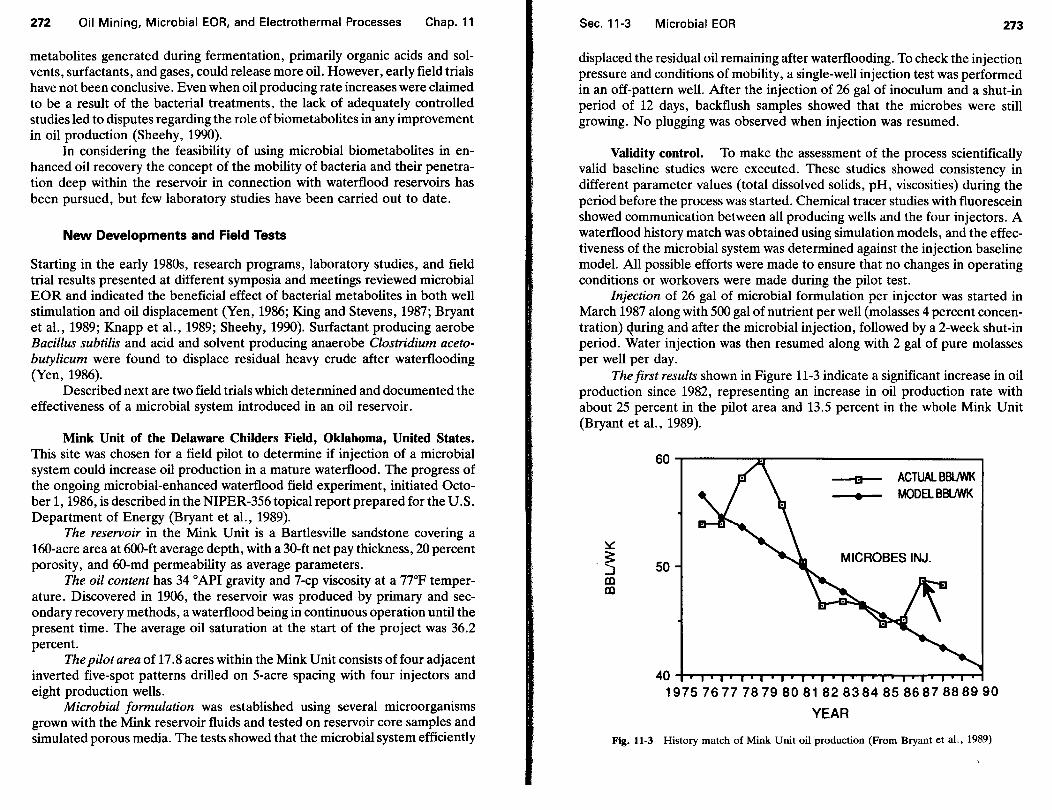
272 Oil Mining, Microbial EOR, and Electrothermal Processes Chap. 11
metabolites generated during fermentation, primarily organic acids and solvents, surfactants, and gases, could release more oil. However, early field trials have not been conclusive. Even when oil producing rate increases were claimed to be a result of the bacterial treatments, the lack of adequately controlled studies led to disputes regarding the role of biometabolites in any improvement in oil production (Sheehy, 1990).
In considering the feasibility of using microbial biometabolites in enhanced oil recovery the concept of the mobility of bacteria and their penetration deep within the reservoir in connection with waterflood reservoirs has been pursued, but few laboratory studies have been carried out to date.
New Developments and Field Tests
Starting in the early 1980s, research programs, laboratory studies, and field trial results presented at different symposia and meetings reviewed microbial EOR and indicated the beneficial effect of bacterial metabolites in both well stimulation and oil displacement (Yen, 1986; King and Stevens, 1987; Bryant et al., 1989; Knapp et al., 1989; Sheehy, 1990). Surfactant producing aerobe Bacillus subtilis and acid and solvent producing anaerobe Clostridium acetobutylicum were found to displace residual heavy crude after waterflooding (Yen, 1986).
Described next are two field trials which determined and documented the effectiveness of a microbial system introduced in an oil reservoir.
Mink Unit of the Delaware Childers Field, Oklahoma, United States. This site was chosen for a field pilot to determine if injection of a microbial system could increase oil production in a mature waterflood. The progress of the ongoing microbial-enhanced waterflood field experiment, initiated October 1, 1986, is described in the NIPER-356topicalreportpreparedforthe U.S. Department of Energy (Bryant et al., 1989).
The reservoir in the Mink Unit is a Bartlesville sandstone covering a 160-acre area at 600-ft average depth, with a 30-ft net pay thickness, 20 percent porosity, and 60-md permeability as average parameters.
The oil content has 34 °API gravity and 7-cp viscosity at a 77°F temperature. Discovered in 1906, the reservoir was produced by primary and secondary recovery methods, a waterflood being in continuous operation until the present time. The average oil saturation at the start of the project was 36.2 percent.
The pilot area of 17.8 acres within the Mink Unit consists offour adjacent inverted five-spot patterns drilled on 5-acre spacing with four injectors and eight production wells.
Microbial formulation was established using several microorganisms grown with the Mink reservoir fluids and tested on reservoir core samples and simulated porous media. The tests showed that the microbial system efficiently
Sec. 11-3 Microbial EOR 273
displaced the residual oil remaining after waterflooding. To check the injection pressure and conditions of mobility, a single-well injection test was performed in an off-pattern well. After the injection of 26 gal of inoculum and a shut-in period of 12 days, backflush samples showed that the microbes were still growing. No plugging was observed when injection was resumed.
Validity control. To make the assessment of the process scientifically valid baseline studies were executed. These studies showed consistency in different parameter values (total dissolved solids, pH, viscosities) during the period before the process was started. Chemical tracer studies with fluorescein showed communication between all producing wells and the four injectors. A waterflood history match was obtained using simulation models, and the effectiveness of the microbial system was determined against the injection baseline modeL All possible efforts were made to ensure that no changes in operating conditions or workovers were made during the pilot test.
Injection of 26 gal of microbial formulation per injector was started in March 1987 along with 500 gal of nutrient per well (molasses 4 percent concentration) 4uring and after the microbial injection, followed by a 2-week shut-in period. Water injection was then resumed along with 2 gal of pure molasses per well per day.
The first results shown in Figure 11-3 indicate a significant increase in oil production since 1982, representing an increase in oil production rate with about 25 percent in the pilot area and 13.5 percent in the whole Mink Unit (Bryant et al., 1989).
50
a ACTUAL BBlJWK MODELBBLJWK
MICROBES INJ.
404-~~~~~~~~~~~~~~~~
1975 76 77 78 79 80 81 82 83 84 85 86 87 88 89 90
YEAR
Fig. 11-3 History match of Mink Unit oil production (From Bryant eta!., 1989)

274 Oil Mining, Microbial EOR, and Electrothermal Processes Chap. 11
The water-oil ratios in all producing wells have dropped below the averages in the baseline period, with some wells showing a significant decrease. The oil viscosity in all wells has not changed significantly, and the surface tension is not lowered enough from the baseline data.
The oil mobilization appears to be caused by the growth of microorganisms in the highly permeable water channels. Their presence blocks the pores, diverts the water to the poorly swept zones and increases the volumetric sweep efficiency.
Alton Field microbial trial, Australia. This field pilot is described in the SPE/DOE 20254 technical paper (Sheehy, 1990) and shows not only the feasibility of stimulating oil production using microbial injection but also the capability of the process to operate at higher reservoir temperatures.
The reservoir in the Alton Field is a Boxvale sandstone covering 1840 acres at 6100-ft average depth with thin sands having average porosity of 17.2 percent and permeability of 260 md.
The original oil in place estimated at approximately 10 MM STB (1.59 x 10⁶ m3
) is a medium light oil on a paraffin base at 169° F (76° C) reservoir temperature. The Alton reservoir was discovered in 1966 and was produced by fluid expansion and a weak water drive. The initial production rate of 1000 bbVday declined, nearing its economic limit of 15 bbVday obtained at present from five wells on a beam pump.
Microbial stimulation has been considered a more viable alternative than expensive waterflood or other EOR methods, since high-risk factors are involved due to the stratified nature of the sands. The high residual oil saturation estimated at 50 percent of the porous volume, the possibility of improving the sweep efficiency of the thin sands, and the desire to generate surfactants in situ sustained the decision to stimulate a producing well with microorganisms.
Detailed laboratory studies and coreflood experiments have been conducted to select and isolate desirable microbial species, to enrich the biometabolites produced in reservoir simulated conditions, and to check the compatibility of introduced microorganisms with the resident reservoir microorganisms.
To assure the validity of the results all evaluations of the effectiveness of the microbial system were determined by comparison with the natural baseline established by a trial shut-in period (point A, Figure 11-4) to log post shut-in production (Sheehy, 1990). Since a workover program was conducted on the Alton #3 well, an injection baseline was also established by injection of production water, followed by well shut-in (point B, Figure 11-4).
Injection of 86 bbl of microbial solution followed by 35 bbl of produced water to displace the system is designated as point Con Figure 11-4. After a 3-week shut-in period, the Altona #3 well was put back into production.
The first results are illustrated in Figures 11-5 and 11-6. As can be clearly observed with reference to the control lines, oil production increased approx-
Sec. 11-3 Microbial EOR
1000.0
+-+ BFPI ...___. BOPD
A, B c ! l l
100.0
" ...,.
\ ._.... v
A, B c
10.0 "" !.A. lfo..o.. !~
'\
BOPD 'II ........
/ J.- Natural Baseline (Stabilized +,niectio+ Test)
Baseline 86 87 BB 89
Fig. 11-4 Graph 1: Production history of Alton no. 3, 1986 to 1990 (Adapted from Sheehy, 1990)
Oil production
20~·-------------------------------,
275
c Q. ----e- Test Oil BPD 11:1 10
- Control Oil BPD
0 0
0 50 1 00 150 200 250 300 350
Day#
Fig. 11-5 Microbial EOR-daily production (From Sheehy, 1990)

276 Oil Mining, Microbial EOR, and Electrothermal Processes Chap. 11
BS&W
----a-- Test BS & W 90
- ControiBS&W
0 50 100 150 200 250 300 350
Day#
Fig. 11-6 Microbial EOR-water cut (From Sheehy, 1990)
imately 40 percent and the watercut was reduced. The result of biological activity in the reservoir was also sustained by the increase in annulus pressure due to C02 and methane accumulation, the increase in the ion level of the production water, the 1000-fold increase in microbial numbers, and a significant decrease (10 to 25 percent) in the water-oil interfacial tension.
Comments. Although there is no given explanation as to how the microbial system injected into the reservoir induced the production of biometabolites, the conclusive results of this field trial are that oil production was beneficially stimulated. However, numerous problems need to be resolved and more research and tests performed in controlled field projects to establish different stimulation technologies and to prove quantitatively that microbial biometabolites can indeed enhance oil recovery.
11-4 ELECTROTHERMAL PROCESSES
Electrothermal processes utilize electricity or electromagnetic energy to stimulate heavy oil reservoirs and tar sands. Several processes have been proposed,
Chap. 11 References 277
and an overview of the existing state of specific technologies is presented by Chute and Vermeylen (1988) and by Pautz and coworkers (1990).
The processes involve heating of the formation to a temperature that will lower the oil viscosity to the point where it can flow or be displaced by steam. This temperature increase is achieved with electromagnetic energy produced by using adjacent wells as electrodes. Reservoirs can also be heated by radio frequency (RF). In this case monopole or dipole antenna structures are introduced downhole to apply RF energy to the reservoir.
Few of these proposed procedures have been tested successfully in the field, and more innovation is needed in the area of electrode design and siting before the process can become commercially viable (Pautz et al., 1990).
QUESTIONS
11-1 Why has interest in underground oil recovery increased only recently (during the last two decades) even though mining for oil is a very old method?
11-2 Describe the oil mining concept.
11-3 What are the characteristics and considerations on which to base the selection of an oil reservoir as a good candidate for underground oil recovery?
11-4 Enumerate some of the most important safety precautions in underground recovery operations.
11-5 Considering the reservoir characteristics, history, and present conditions, explain why applying 10M at the Annona Chalk section of Caddo Pine Island Field would produce more oil from the reservoir.
11-6 What are the biometabolites generated by bacterial activity and how can oil produ~tion be improved by them?
11-7 The microbial stimulation process needs a two- to three-week well shut-in period for fermentation. How can the results obtained be conclusively attributed to microbial stimulation when it is known that a well produces more oil after a period of shut-in time, even without any stimulation process applied?
REFERENCES
ALBAYRAK, F. A., and T. E. PROTOPAPAS, Detailed Technical and Economic Feasibility of Light Oil Mining in the United States, DOE/BC/10704-8 (Washington, D.C.: U.S. Department of Energy, August 1984).
BRYANT, R. S., et al., NIPER-356 Microbial-Enhanced Waterflood Field Experiment, Topical Report, prepared for U.S. DOE under Coop. Agreement No. FC22-83FE60149, NIPER (Bartlesville, OK: U.S. Department of Energy, January 1989).
BRYANT, R. S. et al., "Optimization of Microbial Formulations for Oil Recovery: Mechanism of Oil Mobilization, Transport of Microbes and Metabolites, and Effects of Additives," Society of Petroleum Engineers: Paper SPE 19686 presented at the Annual Technical Conference and Exhibition, SPE 89, San Antonio, Texas, October 8--11, 1989.

278 Oil Mining, Microbial EOR, and Electrothermal Processes Chap. 11
CHUTE, F. S., and F. E. VERMEYLEN, "Present and Potential Applications of Electromagnetic Heating in the In-Situ Recovery of Oil," Vol. 4, no. 1, AOSTRA Journal of Research (1988), pp. 19-33.
ENERGY DEVELOPMENT CONSULTANTS, Mining for Petroleum Feasibility Study, U.S. Bureau of Mines, OFR 56-79, DOE/PB 297133 (July 1978).
GOLDER AssOCIATES, Oil Mining-A Technical and Economic Feasibility Study of Oil Production by Mining Methods, U.S. Bureau of Mines, OFR 55-79, PB 297134 (October 1978).
KING, J. W., MEOR Technical Status and Assessment of Needs-1986, performed for U.S. DOE under Contract No. AC 19-85/BC10852-2, Hardin Simmons University, Abilene, Texas (Bartlesville, OK: U.S. Department of Energy, 1987).
KING, J. W., and D. A. STEVENS, Proceedings of the First International MEOR Workshop, Apri/1-3, 1986, Prepared for U.S. DOE under Contract No. AC 19-85/BC10852-1, Hardin-Simmons University, Abilene, Texas (Bartlesville, OK: U.S. Department of Energy, January 1987).
KNAPP, R. M., et al., Microbial Field Pilot Study, Final Report for the Period Dec. 15, 1986-March 31, 1988, Prepared for U.S. DOE under Contract No. AS 19-86/BC14084-6, University of Oklahoma, Norman (Bartlesville, OK: U.S. Department of Energy, January 1989).
PAUTZ, J. F., P. SARATHI, and R. THOMAS, Review of EOR Project Trends and Thermal EOR Technology, Topical Report, prepared for DOE under Coop. Agreement No. FC 22-83FE60149, by NIPER-461 (Bartlesville, OK: U.S. Department of Energy, March 1990).
RICE, G., "Mining Petroleum by Underground Methods: A Study of Methods Used in France and Germany and Possible Application to Depleted Oil Fields Under American Conditions," Bureau of Mines Bulletin 351 (Washington, D.C.: U.S. Department of Commerce, June 1932).
SHEEHY, A. J., "Field Studies of Microbial EOR," Paper SPE/DOE 20254, presented at the SPE/DOE Seventh Symposium on Enhanced Oil Recovery, Tulsa, Oklahoma, April 22-25, 1990.
STREETER et al., "Recovery of Oil from Underground Drillsites," SPE 19344, 1989 SPE Eastern Regional Conference and Exhibition, Morgantown, West Virginia, October 24-27, 1989.
THAM, M. K., H. B. CARROLL, JR., et al., Improved Oil Mining: A Feasibility StudyFinal Report, NIPER-328, performed under Coop. Agreem. No. FC22-83FE60149 (Bartlesville, OK: U.S. Department of Energy, September 1988).
YEN, T. F., Bacteria Transport Through Porous Media, Annual Report, prepared for U.S. DOE under Contract No. AS19-81/BC10508, University of Southern California, Los Angeles, California, March and September 1986.
Chapter 12
EOR Could Offset Oil Production Decline
12-1 ENERGY CONSUMPTION
The distribution of U.S. energy consumption is shown in Figure 12-1. The pyramid rep~esents the percentage of total U.S. consumption of each energy source provided during 1988 ("Energy Focus," 1989). Petroleum products represent 42.5 percent of total U.S. energy consumption and about half are imported.
The energy forecast through the year 2000 indicates that the United St~tes will remain highly dependent on crude oil since its consumption by the pnmary energy sources that use petroleum liquids will remain constant if not increase.
Growth in coal consumption is projected, but the main sources of nonhydrocarbon energies such as nuclear, hydroelectric, solar, and wind are not considered to have a significant impact in the near future (National Petroleum Council, 1984).
279

280 EOR Could Offset Oil Production Decline
7%
NATURAL GAS 23%
COAL 23.5%
PETROLEUM PRODUCTS 42.5%
Chap. 12
Fig. 12-1 The dynamics of U.S. energy consumption (Adapted from Journal of Petroleum Technology, July 1989)
12-2 ENERGY SUPPLY
Petroleum products are supplied by domestic crude oil production and by foreign sources.
Domestic Crude Oil Production
Existing oil reservoirs. Domestic crude oil production is obtained from existing oil reservoirs which, as hydrodynamic units, are characterized by four productive stages (Figure 12-2):
Stage I. Stage II. Stage III. Stage IV.
Increased production rate as the wells pattern is drilled Peak production rate Sharp decline as reservoir pressure declines Slow decline of the long and final production phase
Even if this scenario is improved by injecting water or gas to supply the reservoirs with energy, only an average of one-third of the original oil in place is recovered. A substantial amount of oil, nearly 325 billion barrels (66 percent of OOIP) remains trapped in the swept areas of existing oil reservoirs or is vypassed by the injected agents.
Sec. 12-2 Energy Supply 281
ID Peak -; cc r::
.5! u :I
"C 0 ... ll.
0
Time
Fig. 12-2 Oil reservoir productive stages
New oil reservoirs. The domestic crude oil production can be maintai~ed at a constant level only if new oil reservoirs are discovered by exploration and recoverable reserves are added annually in the same percentage as they are consumed.
To find, explore, and develop new oil reservoirs for production is much more difficult now than in the past years. The trend of reserve additions per foot of exploration drilling is declining (Figure 12-3).
Today exploration drilling results are less and less attractive (one good well out of seven to nine dry holes), and harsher environments raise the expenses of drilling (National Petroleum Council, 1984). The discovery of any huge new oil field is unlikely.
0 400 0 u. i:;CI IDr:: ~§ 300 gc .!!! r:: 0.5! 200 =Cii 0(; c;o. ..!!! .n 100 ! ii Ill
0
1935 1945 1955 1965 1975 1985 Year
Fig. 12-3 Barrels of oil discovered per foot of exploratory well in United States (From Ivanhoe, 1983)

282 EOR Could Offset Oil Production Decline Chap. 12
Consequences. Domestic crude oil production cannot be maintained, and the major U.S. oil producing states show production declines from peak years (Figure 12-4). Alaska is the only remaining domestic location with oil reservoirs mostly in stages I and II that still have not shown production declines ("Energy Focus," 1987).
Foreign Sources
Future trends. The balance of crude oil needed to satisfy the level of consumption must be met by imports. Since there are still no ready alternatives to petroleum as an energy source and since domestic crude oil production is declining, there will be an even greater reliance on foreign supply.
Lower crude oil prices also lead to higher U.S. dependency on imports, and countries offering the greatest export potential cannot necessarily be considered reliable sources, politically or economically (King, 1987).
As is stated in the federal EOR research report (U.S. DOE, 1985) increased imports are detrimental since they
• will reduce domestic employment, productivity, and economic activity;
• will reduce Federal and State tax bases; • will exacerbate balance of payment deficits; • will increase vulnerability to imporfdisruptions and pressure from exporting
countries; and • the US national economic and military security demands a significant level
of domestic petroleum production.
One example of activity highly dependent on oil prices is the enhanced oil recovery project starts in the last decade (Figure 12-5). As can be observed, the numbers of project starts correspond to the fall of the oil price (Pautz et al., 1990) and are also expected to follow the rise in oil prices beginning with 1990.
12-3 EOR: THE ANSWER FOR OFFSETTING OIL PRODUCTION DECLINE
Enhanced oil recovery can be applied to the already known oil reservoirs to recover more oil that is trapped or unreachable by conventional technology.
The expert in-depth evaluation by the National Petroleum Council (1984) has estimated that EOR could add
• From 7.4to 34 billion barrels (1.176 x 10⁹ to 5.4 x 10⁹ m3) to U.S. reserves
representing 25 to 120 percent of currently proven reserves and • From 600,000 to 2.8 million barrels (25.4 x 10³ to 445.2 x 1Q3 m3
) per day
~ 0 <0 (f)
I 0 0 0 (f)
~ 0 l.t) 'l:f
0 0 0 C'i
I ~ 0 (f)
0 0 0 .....
~ 0 ..... 'l:f
Oil Production (Mbbl/day)
F ~ .... c:o ..... <(
r ~ l.t) 'l:f
J ..... 'l:f
)..
0 r:::
'0-ca ::-.:::
~
>< E ::!
CD ~ :::!!!
z E 0 .::
~ 0 ..... c:o
r::: "0 0
- 0.. "' "0
•o ~ <0 C'i I
E s "' 0 ... "' >- 0
3: ;>,
-"'= "' 0
ca 0..
::;;: 0 (.)
0 I: ·;;; - 0 I:
ii ~ 0
(.) "0
c:~ or-0 ·~ 00
- 0\ ca ~~ <( 0 ...
... 0.. r:>....:t:
ca ~~ "' <::> ....1 cc ~] 0 u ll..~
>< ..,. r:: • ::!
I- ~~ <::> . ....
lOll-r;::~
0
283

NEW PROJECT STARTS
II __ _ ---r --
\
j
--<
lO 0 lO 0 lO M M N N .-i <I> <I> <I> <I> <I>
AVE. DOMESTIC WELLHi:AD OIL PRICE, $/BBL.
284
~ 0) .....
0 w
Chap. 12 References 285
in production (U.S. DOE, 1985), depending on future oil prices and reflecting different degrees of technological advancement.
However, the overall potential for EOR production is highly uncertain since efforts for more research and development activity are disturbed by oil price fluctuations in the low range. To attenuate this oil price stress, the amount of capital and incentives available to the petroleum industry must be increased. We must continue to analyze, understand, and improve the recovery technology of domestic crude oil's potential as the nation's main source of energy. Only then can we be better prepared for the energy needs of the twenty-first century.
REFERENCES
"Energy Focus," Journal of Petroleum Technology (April1987). "Energy Focus," Journal of Petroleum Technology (July 1989), p. 688.
IVANHOE,L. B., "Free World Oil Discovery Indexes-1945-1981," Oil and Gas Journal (November 21, 1983), pp. 88-90.
KING, J. W., MEOR Technical Status and Assessment of Need.s-1986, prepared for, US/DOE under Contract No. AC19-85BC10852-2, Hardin-Simmons University, Abilene, Texas (Bartlesville, OK: US-DOE, March 1987).
NATIONAL PETROLEUM COUNCIL, Enhanced Oil Recovery (Washington, D.C.: NPC, June 1984), pp. 89-91.
PAUTZ, F. S., et al., Review of EOR Project Trends and Thermal EOR TechnologyTopical Report, prepared for DOE by NIPER-461 under Coop. Agreement No. FC 22-83FE60149 by NIPER (Bartlesville, OK: U.S. DOE, March 1990).
U.S. DEPARTMENT OF ENERGY, Federal EO R Research: Increased Understanding of the 300-Billion-Barrel U.S. Residual Oil Resource and the Technologies to Produce lt, DOE/BC-85/6/SP (Bartlesville, OK: U.S. DOE, distribution category UC-92a, October 1985).