author's personal copy - hawaii national marine renewable

Author's personal copy

Wave energy resources along the Hawaiian Island chain

Justin E. Stopa a, Jean-François Filipot a,1, Ning Li a, Kwok Fai Cheung a,*, Yi-Leng Chen b, Luis Vega c

aDepartment of Ocean and Resources Engineering, University of Hawaii at Manoa, Honolulu, HI 96822, USAbDepartment of Meteorology, University of Hawaii at Manoa, Honolulu, HI 96822, USAcNational Marine Renewable Energy Center, University of Hawaii at Manoa, Honolulu, HI 96822, USA

a r t i c l e i n f o

Article history:Received 24 January 2012Accepted 12 December 2012Available online

Keywords:HawaiiSpectral wave modelsMesoscale modelWave atlasWave energyWave power

a b s t r a c t

Hawaii’s access to the ocean and remoteness from fuel supplies has sparked an interest in ocean waves asa potential resource to meet the increasing demand for sustainable energy. The wave resources includeswells from distant storms and year-round seas generated by trade winds passing through the islands.This study produces 10 years of hindcast data from a system of mesoscale atmospheric and spectral wavemodels to quantify the wind and wave climate as well as nearshore wave energy resources in Hawaii.A global WAVEWATCH III (WW3) model forced by surface winds from the Final Global TroposphericAnalysis (FNL) reproduces the swell and seas from the far field and a nested Hawaii WW3 modelwith high-resolution winds from the Weather Research Forecast (WRF) model capture the local waveprocesses. The Simulating Waves Nearshore (SWAN) model nested inside Hawaii WW3 provides data incoastal waters, where wave energy converters are being considered for deployment. The computed waveheights show good agreement with data from satellites and buoys. Bi-monthly median and percentileplots show persistent trade winds throughout the year with strong seasonal variation of the waveclimate. The nearshore data shows modulation of the wave energy along the coastline due to theundulating volcanic island bathymetry and demonstrates its importance in selecting suitable sites forwave energy converters.

� 2013 Elsevier Ltd. All rights reserved.

1. Introduction

The Earth’s changing climate, the increasing cost of oil, andthe finite supply of fossil fuels have created social, economic, andpolitical pressure for alternative sources of energy. Public and pri-vate industries across the globe are actively using, developing, andtesting technologies to extract clean energy. Hawaii’s high con-centration of population and isolated location in the Pacific pro-vides the perfect backdrop for development of renewable energyresources. The state legislature passed the Clean Energy Initiative in2008 with the goal of reaching 70% clean energy by the year 2030.Energy technologies utilizing wind and solar resources are com-mercially available and used across the state. There is a reignitedinterest in oceanwaves as a potential resource for the production ofelectricity in Hawaii. Research and development work on waveenergy conversion (WEC) devices, which had begun much earlier

around the world, has produced many designs and prototypesready for sea trials [1,2]. The devices planned for Hawaii operate inapproximately 50 m water depth outside the surf zone and yet areclose to the shore for mooring and maintenance as well as con-nection to the power grid.

Throughout the world Hawaii is known for its powerful wavesand its marine recreational activities. Hidden in these activitiesare the wave energy resources and the research opportunitiesto understand the ocean environment. The mid-Pacific locationand massive archipelago provide an excellent tapestry to studythe unique wave climate not seen in other places. Fig. 1 illustratesthe climate pattern of the wind waves and swells around the majorHawaiian Islands. The multi-modal sea state in Hawaii provides anindicator of the weather from the far-reaching corners of the Pacific[3]. Extratropical storms near the Kuril and Aleutian Islandsgenerate northwest swells reaching 5 m significant wave heightin Hawaii waters during November through March. The south-facing shores experience more gentle swells generated by theyear-round Westerlies in the Southern Hemisphere that areaugmented by mid-latitude cyclones off Antarctica during Maythrough September [4]. In addition, the consistent trade windsgenerate wind waves from the northeast to east throughout theyear. The Hawaiian Islands modify the trade wind flow and create

* Corresponding author.E-mail addresses: [email protected] (J.E. Stopa), [email protected]

(J.-F. Filipot), [email protected] (N. Li), [email protected] (K.F. Cheung), [email protected] (Y.-L. Chen), [email protected] (L. Vega).

1 Present address: Service Hydrographique et Océanographique de la Marine,Brest CEDEX 2, France.

Contents lists available at SciVerse ScienceDirect

Renewable Energy

journal homepage: www.elsevier .com/locate/renene

0960-1481/$ e see front matter � 2013 Elsevier Ltd. All rights reserved.http://dx.doi.org/10.1016/j.renene.2012.12.030

Renewable Energy 55 (2013) 305e321


localized weather patterns [5]. Knowledge of the regional waveclimate and the coastal wave resources is a prerequisite in the se-lection of suitable sites for testing and operations of wave energyconverters. However, the available buoys as shown in Fig. 1 providewave data either far offshore of the island chain or at nearshorelocations not directly relevant for most potential sites.

Third generation spectral wave models, which can describemulti-modal sea states, have emerged as a reliable tool for fore-casting and hindcasting ocean conditions. Thesemodels account forrandom sea states under the action of winds by evolving the energydensity spectrum in time and space for a range of wave frequenciesand directions. The National Centers for Environmental Prediction(NCEP) operates the third generation spectral wave modelWAVEWATCH III (WW3) to provide 7.5 days of global wave forecastsat 0.5� resolution [6,7]. This operational model is forced withassimilated surface winds from the Global Forecast System (GFS)[8]. The European Centre for Medium Range Weather Forecasts(ECMWF) operates the integrated Forecast System (IFS), whichconsists of an atmospheric model coupled with the spectral wavemodelWAM [9] to produce 10-day forecasts at 0.36� resolution. Theuse of these operational models in hindcast mode allows assess-ment of the global wave climate and energy resources. Caires et al.[10] compiled IFS reanalysis data over the period 1971e2000 toprovide a 1.5� � 1.5� atlas of global winds and waves. Arinaga andCheung [3] produced a 1.25� � 1� global atlas of wind wave andswell energy using WW3 and NCEP’s Final Global TroposphericAnalysis (FNL) winds from 2000 to 2009.

The resolution in the global wave models prevents properdescriptions of the wave conditions near the shore and can lead tosignificant errors along an archipelago as demonstrated by Poncede Leon and Guedes Soares [11] and Rusu et al. [12]. Recent studieshave used spectral wave models at higher resolution with

interpolated global wind data to provide assessment of regional orcoastal wave resources in Europe [13e15], North America [16,17],and Australia [18]. The Hawaii archipelago, however, modifies thetrade wind flow and creates localized weather patterns that mustbe considered in spectral wave modeling. Stopa et al. [19] utilizeda two-way nested global and Hawaii WW3 model to examine theeffects of local winds on wave energy resources in two case studiesrepresentative of winter and summer conditions. The FNL dataprovides the global wind forcing as well as the initial and boundaryconditions to produce high-resolution regional winds from theWeather Research and Forecast (WRF) model [20]. The Hawaii WRFmodel describes mesoscale phenomena such as diurnal thermalforcing of sea and land breezes [21], flow acceleration and decel-eration around topographic features, and wake formation on theleeside of islands [5]. The speed-up of the winds in channels andaround headlands augments the far-field wave energy and createswave conditions that are known to be treacherous to mariners.

The present study continues the effort of Stopa et al. [19] andArinaga and Cheung [3] by utilizing the Simulating WAves Near-shore (SWAN) model of Booij et al. [22] at each major island in

Fig. 1. Wave climate, buoy resources, and nested computational domains around the Hawaiian Islands.

Table 1Setup of nested computational domains for spectral wave modeling.

LowerLon.(�E)

UpperLon.(�E)

LowerLat.(�N)

UpperLat.(�N)

Resolution (�) Resolution(km)

Global WW3 0.00 360.00 �90.00 90.00 1.25 � 1.00 138 � 111Hawaii WW3 199.00 207.00 17.00 24.00 0.05 � 0.05 5.6 � 5.6Kauai SWAN 199.65 200.80 21.70 22.35 0.005 � 0.005 0.56 � 0.56Oahu SWAN 201.65 202.40 21.20 21.75 0.005 � 0.005 0.56 � 0.56Maui SWAN 202.60 204.10 20.40 21.30 0.01 � 0.01 1.1 � 1.1Hawaii SWAN 203.80 205.30 18.85 20.35 0.01 � 0.01 1.1 � 1.1

J.E. Stopa et al. / Renewable Energy 55 (2013) 305e321306


Hawaii and extending the hindcast study to provide a continuousdataset from 2000 to 2009. The high-resolution Hawaii WW3accounts for local winds and island shadowing to provide an ac-curate description of the complex wave pattern along the islandchain. The SWAN model is better suited for nearshore environ-ments due to the implicit numeric scheme and the ability to ac-count for triad wave interactions in shallow water. It can accountfor some effects of diffraction by including an additional termderived from the mild-slope equation [23]. Filipot and Cheung [24]recently provided additional parameterizations of energy dis-sipation due to wave breaking and bottom friction for the fringingreef conditions of Hawaii. Wind and wave data derived from sat-ellite and buoy measurements allows validation of the hindcastWRF and WW3 data around Hawaii. The 10 years of validatedhindcast data provides a wealth of information to elucidate thewind and wave climate and develop high-resolution wind andwave atlas in Hawaii. The nearshore data from SWAN describes thewave energy resources in the form of bi-monthly median andpercentile plots to provide precise information for planning anddesign of wave energy converters along the island coasts.

2. Methodology

2.1. Model setup

The present study utilizes a system of nested global, regional,and island-scale spectral wave models based on WW3 of Tolmanet al. [6,7] and SWAN of Booij et al. [22] with wind forcing from theNOAA Final Global Troposphere Analysis (FNL) and a WRF modelresolving the major Hawaiian Islands. Fig. 1 illustrates the setup ofthe nested wave models. Four island-scale SWAN domains arenested within the Hawaii WW3 domain, which in turn is nestedinside a global WW3 domain. Table 1 lists the coverage and reso-lution of each computational grid. The series of nested grids capturephysical processes at increasing temporal and spatial resolutiontoward Hawaii. The system is automated through a set of scripts,which link the model components with databases and utilityprograms to provide high-resolutionwind andwave data. The samesystem is also in operation to provide 7.5-day high-resolutionforecasts of wind and wave conditions around Hawaii (http://oceanforecast.org/).

The key to the entire modeling process is accurately describingthe input wind field. The Global Forecast System (GFS) is a spectralmodel with 0.5� spatial resolution on the earth surface and 64layers extending to the top of the atmosphere [8]. NCEP runs themodel four times daily with assimilation of observational data fromland stations and satellites to forecast the atmospheric conditionson a real-time basis [25]. The FNL data, which is derived from GFSon a 1� �1� grid at 0000, 0600, 1200, and 1800, provides the initialand boundary conditions to Hawaii WRF [26]. The WRF model isbased on the non-hydrostatic, three-dimensional Euler equation inthe sigma vertical coordinate. In the regional implementation, theNoah LSM (NCEP, Oregon State University, Air Force, and Hydro-logical Research Laboratory Land Surface Model) accounts forvegetation coverage and land surface properties using data com-piled by Zhang et al. [26]. The computational domain extends from194e210�E and 16e26�N beyond Hawaii WW3 to model the up-stream flow from the trade winds and the modified wind fielddownstream of the islands. The 6 km grid spacing is sufficient toresolve the physical processes important to local wind wave gen-eration. The production consists of a series of overlapping 36-h runswith the data output at the standard 10m elevation every hour. Thefirst 12 h allows spin-up of the regional model from the boundarycondition and the remaining 24 h is archived to produce a con-tinuous 10-year dataset of the wind velocity.

WW3 is a third generation spectral wave model developed byTolman et al. [6,7]. The phase-averaged model evolves the actiondensity N for a range of frequencies f and 360� of directions q underwind forcing and geographical constraints. It is governed by theaction balance equation and when written in the latitude andlongitude (x, j) spherical coordinates, is given by

vNvt

þ 1cos x

v

vx_xNcos qþ v

vj_jN þ v

vk_kN þ v

vq_qN ¼ S

s(1)

where t denotes time, k is wave number, s ¼ 2pf is intrinsic angularfrequency, the over-dot represents the rate of change, and S denotesthe source terms accounting for nonlinear effects such as windewave interactions, quadruplet waveewave interactions, dissipationthrough whitecapping, and dissipation due to bottom friction. TheWAM4 source terms [27], which are available in the latest release ofWW3 (V3.14), are applied to account for these nonlinear processes.The directional wave energy spectrum is obtained from F(f,q)¼ N(k,q)/s through a Jacobian transform from k to f. The significantwave height and average period are defined as

Hs ¼ 4

ffiffiffiffiffiffiffiffiffiffiffiffiffiffiffiffiffiffiffiffiffiffiffiffiffiffiffiffiffiffiffiffiffiffiffiffiZN

0

Z2p

0

Fðf ; qÞdqdf

vuuut (2)

T02 ¼ffiffiffiffiffiffiffim0

m2

r(3)

where m0 and m2 are the zeroth and second moment of the waveenergy spectrum. We implement Global WW3 at 1� � 1.25� reso-lution and incorporate a nested Hawaii grid at 30 (w5.5 km) reso-lution. An obstructions file accounts for energy lost at small islandsthat cannot be resolved in the global computational grid [28]. FNLprovides a continuous dataset of wind velocity and ice coverageat six hours intervals for input into Global WW3. Spectral waveconditions are exchanged internally at the boundary of HawaiiWW3, which is forced by hourly Hawaii WRF winds to capture thelocal wave conditions.

The Hawaii WW3 defines the spectral boundary conditions forSWAN to model coastal wave transformation in four island-scaledomains as shown in Fig. 1. The resolution of the computationalgrids ranges from 1800 (0.55 km) for Kauai and Oahu to 3600 (1.1 km)for Maui and Hawaii Island. High-quality bathymetry aroundthe islands is available from LiDAR surveys at 3e4 m resolutiondown to 40 m depth and from multibeam surveys at 50 m reso-lution in deeper waters. SWAN is similar to WW3 in that it solvesthe action balance Eq. (1) with parameterization of nonlinearprocesses, but its implicit scheme provides a steady state solutionat each time step. The model includes additional source terms fortriad waveewave interactions, depth-induced wave breaking,wave diffraction, and dissipation in beach and reef environments.The SWAN domains provide the wave power in coastal watersusing

P ¼ rgZN

0

Zp

�p

Cgðf ÞFðf ; qÞdqdf (4)

where r is the density of water, g is the acceleration due to gravity,Cg is group velocity. The wave climate in Hawaii always containsamix of swells andwindwaves; thus, this method provides a betterrepresentation of the wave power in comparison to the commonapproach of using a single wave height and period estimated fromthe wave spectrum.

J.E. Stopa et al. / Renewable Energy 55 (2013) 305e321 307


2.2. Observational data for validation

The FNL wind data, which already includes available measure-ments, underwent extensive evaluations prior to its releases [8].Arinaga and Cheung [3] implemented the data in Global WW3 andvalidated the computed wave parameters with satellite and buoymeasurements around the globe. The high-resolution, regionalwind and wave data produced in this study needs independentvalidation with actual measurements before its implementation inthe resource assessment. Fig. 1 shows the locations of seven off-shore and five nearshore buoys operated by the National Data BuoyCenter (NDBC) and the University of Hawaii (UH). These buoysprovide direct and continuous measurements of the wave condi-tions for comparison with the model output at discrete locationsaround Hawaii. Spatial data available for model validation includeswind measurements from QuikSCAT and altimetry wave mea-surements from Jason-1. These platforms provide valid measure-ments across a large spatial region under most atmosphericconditions.

QuikSCAT provides wind measurements over 90% of the ice-freeocean surface daily with errors of less than 2m/s in speed and 20� indirection [29]. The polar orbiting satellite flies over Hawaii twicedaily in ascending and descending passes. The 1800-km swath,which covers most of the island chain, has a nominal spatial reso-lution of 12.5 km to capture mesoscale features. The scatterometeron QuikSCAT pulses cloud-penetrating microwaves in the Ku bandtoward the earth and records the backscatter signal under amajorityof weather conditions. The wind speed and direction at 10-melevation can be estimated from an empirical relationship knownas the Geophysical Model Function without taking into accountsecond-order geophysical effects such as wave height and sea sur-face temperature. A land mask of at least 25 km removes erroneousvalues caused by coastal land and a multidimensional rain-flaggingtechnique indicates the presence of rain, which may alter the mi-crowave pulse and subsequently the recorded data. The DirectionInterval Retrieval with Threshold Nudging technique gives a uniquesolution for the wind direction [30]. Gridded wind speeds ofapproximately 12.5 kmprovide a comparisonwith interpolated datafrom Hawaii WRF.

NASA’s Jet Propulsion Laboratory (JPL) operates the Jason-1satellite, which has been providing continuous global oceanconditions since December 2001. The polar orbiting satellitecovers the earth surface from 66�S to 66�N in 254 passes every 10days. A dual-frequency (C & Ku microwave bands) altimetermeasures the sea surface elevation with errors of up to 3.9 cm.Other on board sensors correct for vapor and electron contents inthe atmosphere and the ionosphere. Erroneous data near thecoastlines due to contaminated signals by the presence of land areremoved when appropriate. The significant wave height is anintrinsic property of the sea surface measurement and is esti-mated from the leading edge of the returned signal with errors of�0.4 m or 10% of the significant wave height, whichever is larger[31]. A number of data products are available through the JPLPhysical Oceanography Distributed Active Archive Center. Thisstudy utilizes the Geophysical Data Record, which is consideredthe most accurate because it is a fully validated product withprecise orbits, rain flags, and corrections for instrument effects.Along-track, gridded Hs values with resolution of approximately 3arcmin (w5.5 km) allow direct comparison with results fromHawaii WW3.

We use a number of error metrics to measure the differencebetween the observed and computed data within the Hawaii WRFand WW3 domains. These include the mean error or bias (ME),normalized root mean square error (NRMSE), correlation (COR),and scattered index (SI) given as

ME ¼ 1N

XNi¼1

ðXPi � XOiÞ (5)

NRMSE ¼PN

i¼1ðXPi � XOiÞ2Nðmax ðXOÞ �min ðXOÞÞ

(6)

COR ¼PN

i¼1

�XPi � XP

��XOi � XO

�ffiffiffiffiffiffiffiffiffiffiffiffiffiffiffiffiffiffiffiffiffiffiffiffiffiffiffiffiffiffiffiffiffiffiffiffiffiffiPN

i¼1

�XPi � XP

�2r ffiffiffiffiffiffiffiffiffiffiffiffiffiffiffiffiffiffiffiffiffiffiffiffiffiffiffiffiffiffiffiffiffiffiffiffiffiffiffiPNi¼1

�XOi � XO

�2r (7)

SI ¼ 1XO

ffiffiffiffiffiffiffiffiffiffiffiffiffiffiffiffiffiffiffiffiffiffiffiffiffiffiffiffiffiffiffiffiffiffiffiffiffiffiffiffiffiffiffiffiffiffiffiffiffiffiffiffiffiffiffiffiffiffiffiffiffiffiffiffiffiffiffiffi1N

XNi¼1

hðXPi � XOiÞ � ðXP � XOÞ

i2vuut (8)

where the over bar denotes themean, the subscripts O and P denoteobserved and computed data, and N denotes the number of datapairs. It should be reiterated that the observed data also containserrors and is simply used as a reference for comparison.

3. Winds in Hawaii

The main Hawaiian Islands, which extend from 19�N to 23�N,lie within the trade wind belt and experiencewinds throughout theyear from the east to northeast [4]. The speed-up of the winds inthe channels and around headlands modifies the wave energy nearthe coast. Before the climate patterns are discussed, the HawaiiWRF data is examined against available wind measurements.QuikSCAT, which flew over Hawaii 7914 times (with sufficient data)during the 10-year period, provides a comprehensive dataset forvalidation.

The WRF winds are interpolated in time and space to matchthose of QuikSCAT for computation of the error metrics. Fig. 2displays the results for the 10 years of wind data. Hawaii WRFprovides a good description of thewind field upstream of Hawaii, inthe channels, and around headlands that is critical for local wavegeneration. In these areas, the mean error and the NRMSE aretypically less than 0.5 m/s and 5%. The computed and observed datashows good correlation of 0.8 and little variability as indicated bya scatter index of 15%. The most significant discrepancy occurs inthe wake region of Hawaii Island, where the simulated wind speedis up to 3.5 m/s or 22% lower than the QuikSCAT winds at theseparation points. The low correlation and large variability implythe errors in the location and timing, instead of the strength, of thecirculation. A deterministic model might not capture the stochasticprocesses in the wake. On the other hand, it is well known thatQuikSCAT overestimates wind speed under weak and variableconditions and produce less reliable measurements in coastal wa-ters. The nominal 12.5-km resolution of QuikSCAT is inadequate indescribing the complex flow pattern in the wake [32e34], butnevertheless, such flow pattern is not conducive to wavegeneration.

Fig. 3 plots the bi-monthly median wind speed to illustrate thelocal weather pattern and its seasonal variation. The trade windspersist throughout the year with the strongest and most consistentperiod in the summer months, peaked at July and August. Thepresence of the islands cause deceleration of the trade wind flow onthe windward shores, while the channel-parallel pressure gradientsaccelerate the flow downstream, especially in the ‘Alenuihahachannel between Maui and Hawaii Island [19]. For mountains withpeaks well above the trade wind inversion, such as Mauna Kea andMauna Loa of Hawaii Island, orographic blocking generates distinctwakes on the leeside with a westerly return flow between a pair of



Fig. 2. Error metrics of wind speeds from Hawaii WRF and QuikSCAT.

Fig. 3. Bi-monthly median wind speed from Hawaii WRF.



Fig. 5. Error metrics of significant wave heights from Hawaii WW3 and Jason-1.

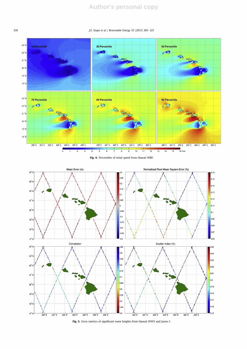
Fig. 4. Percentiles of wind speed from Hawaii WRF.



counter-rotating lee vortices [32,33]. For smaller islands withmountain peaks well below the trade wind inversion, such as Kauaiand Oahu, the wake zone is characterized by relatively weak winds;westerly flow only occurs in the coastal region during the daytime inresponse to land surface heating [33]. The winter months fromNovember through February are susceptible to more variable tradewinds due to the southward shift of the sub-tropical high pressuresystem toward Hawaii and occurrences of winter “Kona” storms[26,35]. These storms are infrequent and are not reflected in themedian plots; however weakened wind speeds in these months areevident.

Wind speed statistics provide additional insights into the localclimate and its effects on the wave resources. Fig. 4 presents the 10,30, 50, 70, 80, and 90 percentiles of the computed wind speed. Theresults depict predominant tradewind flows from east to northeastwith gradual strengthening in each successive percentile plot.The 50-percentile plot is very similar to the median MayeJuneconditions with typical speeds of 8e12 m/s. All of the plotsindicate up to 50% increase of the wind speeds on the north andsouth sides of the islands in relation to the upstream flow. The 90-percentile shows 14 m/s wind speeds in the channels and strongerwinds extending leeward of Hawaii Island. The sufficiently highwind speed and long fetch can have an impact on the local waveenergy during most of the year. The calm wake region extendsacross the entire domain. Effects from this wake have a lastingimpact on the airesea interaction 3000 km beyond the Hawaii ar-chipelago [36].

4. Waves in Hawaii

The 10 years of hindcast data provides a wealth of informationfor wave climate research and resources assessment. Since Arinagaand Cheung [3] have already validated and examined the globalwave data, we focus on the high-resolution data around Hawaii.The hindcast wave data is first validated with satellite and buoymeasurements.We then present bi-monthlymedian and percentileplots of the significant wave height and average period to illustratethe wave climate in Hawaii.

4.1. Validation

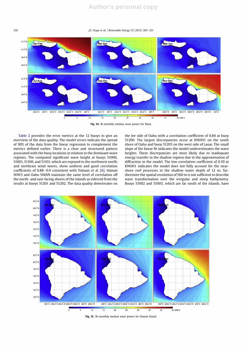
The Jason-1 satellite flew across the Hawaii WW3 domain2243 times (with sufficient data) during the 10-year period. Thecomputed significant wave height is interpolated in time and spaceto compare with the altimetry measurements. Records from gridcells close to land may contain errors, but are included to assess themodel performance in the under-sampled regions at the channelsand near headlands. Fig. 5 plots the error metrics computed alongthe satellite tracks. The results show good agreement of thecomputed and measured data north of the island chain, which are

Table 2Buoy information and error metrics.

Buoy Domain Start time End time Depth (m) �Error (m) ME (m) RMSE (m) NRMSE (%) COR SI (%) Lin. fit slope

51001 Global WW3 Jan-02, 2000 Dec-24, 2009 3430 0.56 0.08 0.38 0.05 0.90 0.16 0.8351002 Hawaii WW3 Jan-02, 2000 Dec-31, 2009 5002 0.59 0.11 0.39 0.07 0.80 0.15 0.8151003 Hawaii WW3 Jan-02, 2000 Dec-31, 2009 4920 0.58 0.1 0.38 0.07 0.81 0.17 0.8251004 Global WW3 Jan-02, 2000 Oct-07, 2009 5082 0.41 0.02 0.29 0.06 0.87 0.12 0.7551100 Hawaii WW3 Apr-24, 2009 Dec-31, 2009 4755 0.56 0.26 0.44 0.08 0.89 0.16 0.8851101 Global WW3 Feb-21, 2008 Dec-31, 2009 4792 0.63 0.26 0.49 0.07 0.88 0.19 0.8251000 Hawaii WW3 Apr-24, 2009 Dec-31, 2009 4097 0.64 0.24 0.47 0.09 0.89 0.17 0.8951200 Hawaii WW3 Oct-10, 2009 Dec-31, 2009 3150 0.60 0.28 0.47 0.11 0.84 0.18 0.8651201 Oahu SWAN Sep-08, 2004 Dec-31, 2009 198 0.54 0.09 0.35 0.06 0.90 0.2 0.9251202 Oahu SWAN Sep-08, 2004 Dec-30, 2009 100 0.43 0.09 0.29 0.06 0.89 0.14 0.8651203 Maui SWAN Jul-01, 2007 Dec-31, 2009 201 0.36 0.11 0.26 0.07 0.67 0.27 0.70KNOH1 Oahu SWAN Sep-01, 2008 Dec-31, 2009 12 0.30 0.09 0.23 0.09 0.59 0.28 0.60

Fig. 6. Comparison of computed and recorded significant wave heights at repre-sentative buoys.



Fig. 7. Wave height validation with buoy measurements.



directly exposed to the north swell and wind waves. The mean andnormalized root mean square errors are within �0.3 m and lessthan 10%. The correlation is above 0.9 and the scattered index iswithin 15%. Larger discrepancies, however, exist in the southernportion of the domain and in the channels. Correlation of 0.7, which

is typical southeast of Kauai and southwest of Oahu and Maui,might be due to the lack of diffraction in WW3 to describe theenergy in the shadows of the northwest swells and northeast windwaves. The track along the ’Alenuihaha Channel shows the lowestcorrelation with a negative bias. The errors are attributed to the

Fig. 8. Bi-monthly median significant wave height from Hawaii WW3.

Fig. 9. Bi-monthly median average wave period from Hawaii WW3.



poorly resolved location and timing of the circulation in the tradewind wake leeward of Hawaii Island. This results in shifting of thewave field and energy level in time and space.

Measurements from 12 buoys around Hawaii are available tovalidate the hindcast data. Table 2 lists the buoy locations, water

depths, and data periods ranging from 1 to 10 years. Fig. 6 plotsa sample of the recorded and computed significant wave heights atfour representative buoys for JanuaryeApril 2005, during whichHawaii experienced several north swell and wind wave events.Buoy 51001 is fully exposed to the northwest swells approaching

Fig. 10. Percentiles of significant wave heights from Hawaii WW3.

Fig. 11. Percentiles of average wave periods from Hawaii WW3.



Hawaii, while buoy 51003 is located in the open ocean to the south.The swells show a general decline in height from north to southacross the island chain. Buoy 51201 at 198 m water depth off thenorth shore of Oahu is partially sheltered from the northwest swellby Kauai and recorded slightly lower or similar wave height com-paring to buoy 51003 to the south. Buoy 51202 at 100 m waterdepth east of Oahu is slightly sheltered from the northwest swells,but fully exposed to the northeast wind waves. The model re-produces the height and timing of the swells and wind waves aswell as the slight attenuation of the swell energy from north tosouth, but underestimates the short duration peak of extremeswells, probably due to the temporal resolution of the FNL data at 6-h intervals. This, however, should have negligible effects on thewave statistics.

Due to the large volume of data, scatter and quantileequantile(QeQ) plots are used along with bulk statistics to describe theerrors at each buoy. Fig. 7 shows the scatter and QeQ plots of the

data at the four representative buoys for the entire period of 10years. The linear regression fit in the scatter plots has a slope of lessthan one, and is consistent with published results in the Pacific [6].The two blue lines delineate 90% of the data, which is typicallywithin �0.6 m of the linear regression. The contours, which denotethe data density, confirm a general decrease of the wave heightacross the island chain from north to south. The QeQ plot, whichsorts the recorded and computed wave heights, shows the twodatasets follow very similar statistical distributions up to 4e5 msignificant wave height. The model tends to underestimate thelarger swells at buoys 51001, 51201, and 51202. This might beassociated with the low temporal resolution of the input FNL windsthat results in omission of short episodic events as illustrated inFig. 6. The slight overestimation at 51003 is likely due to errorscaused by the obstruction coefficients [28], which empirically ac-count for the wave energy reduction through the northwest Ha-waiian Islands in Global WW3.

Fig. 12. Bi-monthly median wave power for Kauai.

Fig. 13. Bi-monthly median wave power for Oahu.



Table 2 provides the error metrics at the 12 buoys to give anoverview of the data quality. The model errors indicate the spreadof 90% of the data from the linear regression to complement themetrics defined earlier. There is a clear and structured patternassociatedwith the buoy locations in relation to the dominant waveregimes. The computed significant wave height at buoys 51000,51001, 51100, and 51101, which are exposed to the northwest swellsand northeast wind waves, show uniform and good correlationcoefficients of 0.88e0.9 consistent with Tolman et al. [6]. HawaiiWW3 and Oahu SWAN maintain the same level of correlation offthe north- and east-facing shores of the islands as inferred from theresults at buoys 51201 and 51202. The data quality deteriorates on

the lee side of Oahu with a correlation coefficient of 0.84 at buoy51200. The largest discrepancies occur at KNOH1 on the southshore of Oahu and buoy 51203 on the west side of Lanai. The smallslope of the linear fit indicates the model underestimates the waveheights. These discrepancies are most likely due to inadequateenergy transfer in the shadow regions due to the approximation ofdiffraction in the model. The low correlation coefficient of 0.59 atKNOH1 indicates the model does not fully account for the near-shore reef processes in the shallow water depth of 12 m; fur-thermore the spatial resolution of 560m is not sufficient to describewave transformation over the irregular and steep bathymetry.Buoys 51002 and 51003, which are far south of the islands, have

Fig. 14. Bi-monthly median wave power for Maui.

Fig. 15. Bi-monthly median wave power for Hawaii Island.



similar correlation coefficients of 0.80 and 0.81 respectively. Thelower correlation in comparison to their northern counterparts islikely due to the use of the obstruction coefficients to account forthe northwest Hawaiian Islands in Global WW3. The higher cor-relation coefficient of 0.87 at buoy 51004 east of Hawaii Islandappears to support this hypothesis.

4.2. Wave climate

The wave climate in Hawaii is defined by the north and southswells superposed on the year-round northeast wind seas. Fig. 8plots the bi-monthly median significant wave heights from the 10years of hindcast data to illustrate the seasonal patterns. Thenorthwest swells dominate the winter months from November toFebruary with typical significant wave heights of 3 m. The islandchain creates a pronounced shadow of the swell energy. The tran-sition months of MarcheApril reveal similar wave patterns with

smaller median wave heights of 2.5 m. During the summer monthsfrom May to August, Hawaii experiences gentle south swells. Theyear-round wind waves of 1e2 m from the northeast produce well-defined shadows on the leeward coasts. Local acceleration of thetrade winds increases the wave height in the channels and to thesouth of Hawaii Island. Local maxima of the wave height developdownstream of the ’Alenuihaha channel and southwest of HawaiiIsland in response to the heightened wind speeds in July and Au-gust. Subtle effects from the south swells are seen in the waters justnorth of the Ka’ie’ie Waho channel, between Kauai and Oahu, theKa’iwi channel, between Oahu and Molokai, and to the east ofHawaii Island, where the larger wave heights are created by com-bining with the wind waves. SeptembereOctober sees an overallincrease in wave height due to a more direct approach of the southswells as the source shifts westward toward New Zealand [4]. Inaddition, the Northern Hemisphere has increased swell activities,although small in relation to the JanuaryeFebruary episodes. There

Fig. 16. Percentiles of wave power for Kauai.

Fig. 17. Percentiles of wave power for Oahu.



are no dominant patterns in these months but a combination of allthree major components.

The wave period plays an equally important role in defining theavailable energy resources. While the peak period is commonlyused to characterize sea states with a dominant component, weconsider the average period, which is more representative of themulti-modal wave climate in Hawaii. Fig. 9 plots the bi-monthly

median wave period to provide a different perspective on thewave climate. The northwest swells dominate the pattern in thewinter months from November to February with average waveperiods over 10 s in exposed waters. The waves generated by thetrade winds have shorter periods of 7e8 s as evident in waters offthe south-facing shores sheltered from the northwest swell. Localacceleration of the trade winds southwest of Hawaii Island results

Fig. 18. Percentiles of wave power for Maui.

Fig. 19. Percentiles of wave power for Hawaii Island.



in heightened wind wave activities and reduction of the averageperiod over a large region. The west-facing shores, which aresheltered from the trade wind waves, see larger periodsassociated with the northwest swells. The increase off the westside of Hawaii Island, which is also in the shadow of thenorthwest swells, is due to the year-round swells generated inthe South Pacific. These local increases of the average period persistthrough the transition months of March and April. In the absence ofthe northwest swells, the effects of the south swell become morevisible with typical wave periods of 6e9 s from May throughAugust. The lower end of the range corresponds to the windwave period in the shadows of the south swells and the upperend represents the average between the south swells and thewind waves. SeptembereOctober represents similar features ofall seasons and no one wave regime dominates.

Figs. 10 and 11 show the percentile plots to illustrate the overallstatistics of the significant wave height and average wave period.The 50-percentile, which has a similar pattern as MayeJune, rep-resents a transition from windewave to north swell dominatedconditions. The most prominent feature is a relatively calm regionextending from Kauai to Hawaii Island due to sheltering from boththe trade wind waves and northwest swells. The northwest swellsdominate the top 30% with significant wave heights and averageperiods larger than 2.5 m and 10 s respectively. The same patternexists in the bi-monthly plots, where the period is enhanced in theswell dominated regions of the northwest shores of Niihau, Kauai,and Oahu. The waves in the ’Alenuihaha channel, which aredominated by local acceleration of the tradewinds, have an averageperiod of 6e8 s 70% of the time. The wave period and significantwave height reach 10 s and 3 m at the 90-percentile confirming theseverity of the wind waves in this region. The wave period patternsreveal the presence of south swells produced in the “RoaringForties” throughout the year [3,4]. Over 90% of the time, the watersslightly west of Hawaii Island experience waves of less than 1.5 mheight, but over 11 s period due to swells from the south. Thewindward shores have wave heights and periods over 2 m and 7 sin comparison. The plots of significant wave height do not showdrastic effects of the south swells, which are being overshadowedby the more energetic northwest swells or northeast wind waves.

5. Wave energy resources

The climate analysis has illustrated the seasonal and regionalpatterns of the wind waves and swells and provided a generalassessment of the potential for wave energy development inHawaii. Site selection is a more delicate design and planning issuebecause of infrastructure investments and regulatoryrequirements. Most pre-commercial WEC devices, such as Pelamisand Power Buoy, are designed for nearshore waters around 50e70 m depth to minimize transmission losses and allow forroutine maintenance. For implementation in Hawaii, it iscurrently expected that these devices will require 5 kW/m ofwave power to be operational and an annual median of 12 kW/mto be viable. High-resolution estimates of wave power in coastalwaters are necessary to identify optimal sites that satisfy theserequirements for deployment of WEC devices.

Eq. (2) provides the wave power in coastal waters around themajor Hawaiian Islands using SWAN output. Figs. 12e15 show thebi-monthly median wave power in the Kauai, Oahu, Maui, and,Hawaii Island domains from the 10 years of hindcast data. BetweenNovember and February, the exposed north shores of all islandsreceive at least 30 kW/m of wave power from the northwest swells.Most of these shorelines have values above 25 kW/m between the50- and 70-m depth contours. Wave refraction over the undulatingvolcanic island slopes modulates the wave energy distribution

Fig. 20. Frequency of occurrence for P � 12 kW/m. White line indicates the 50-mdepth contour.



along the shore. The wave energy resource for the remainder of theyear is moderate despite the year-round northeast wind waves andsouth swells. The northeast wind waves produce consistent powerof 10e15 kW/m between the 50- and 70-m contours of the wind-ward shores from May to October. The south swells are only dis-cernible in the channels between Niihau, Kauai, and Oahu, but notat other locations because they typically have lower energy levelsthan the wind waves. Stopa et al. [19] showed through partitioningof energy spectra that a large south swell only has 15 kW/m of wavepower.

Figs.16e19 showthepercentile plots to illustrate thewavepowerstatistics for planning and operation. The 10-percentile plots, whichshow relatively uniform power of 5 kW/m over all shorelines, arerepresentative of the gentle south swells and moderate trade windwaves in the summer months. The persistent power above thethreshold assures year-round operation of most devices in Hawaii.The 30 and 50 percentiles see increasing contributions of the tradewind waves to the power on the east-facing shores. The north- andeast-facing shores generally have annualmedian power of 15 kW/mor higher between the 50- and 70-m depth contours. The contrast isstriking with the 70, 80, and 90 percentiles, which show dramaticnorthesouth asymmetry of the wave energy distribution. Thesignature of the northwest swells dominates these upper percen-tiles with 30 kW/m or higher on north-facing shores, except forHawaii Island, which is partially sheltered by Maui. The 90-percentile plots show 60 kW/m of wave power at selected loca-tions on Kauai and Oahu’s north shores, where the underlying ba-thymetry focuses the wave energy toward the shore.

All renewable energy technologies face difficulties in producingbase load power to customers. Although the episodic northwestswells produce high wave power, a consistent energy supply is thekey to a successful operation. For illustration, Fig. 20 shows thepercentage time when the wave power is over 12 kW/m for eco-nomic viability. The southern and western shores on all islands aretypically not suitable forWEC devices. It is primarily the year-roundwind waves that supply the most consistent energy within the 50-and 70-m depth contours on north- and east-facing shores. Themost favorable location on Hawaii Island is Cape Kumukahi, whichhas 12 kW/m of wave power 82% of the time. Because of the steepvolcanic island slope, the 50-m contour is within 100 m from theshore at this location. The east Maui coast near Hana, the northMolokai coast at Kalaupapa, and the north Kauai coast at Heanaall have 12 kW/m of wave power for at least 60% of the time. Theselocations have isolated communities that depend on remote ex-tensions of the power grids, thereby making small-scale renewableenergy projects an attractive option.

Oahu has 75% of the state’s population and consumes the ma-jority of electricity produced in Hawaii. The island is home topopulation centers, business districts, tourist destinations, andmilitary installations. Being close to the consumers is a majorincentive to any energy resource project. The insular shelf offKaneohe on the windward shore of Oahu appears to be a favorablesite for wave energy development. The coastline is adjacent toa military base on a headland off the vantage point from nearbycommunities. A region of the insular shelf between the 50- and70-m contours has 12 kW/m of wave power close to 58% of thetime. The site is sheltered from the most severe northwest swellsthat might damage the devices and their mooring systems, whilebeing open to the more gentle, late-season winter swells from thenorth. The location has been selected as the Wave Energy Test Siteof the Hawaii National Marine Renewable Energy Center with testplatforms, mooring systems, power cables, and monitoring buoysextending to about 80 m water depth. The insular shelf off KeanaPoint and Kahuku Point at the northwest and northeast corner ofOahu has 12 kW/m of wave power 55% of the time, but the locations

are open to the severe northwest swells that reach 5 m significantwave height every year.

6. Conclusions

A hindcast study using a system of nested computational modelshas produced 10 years of regional wind and wave data for climateresearch and resources assessment in Hawaii. The computed winddata reproduces the omnipresence of the trade winds in Hawaii andthe local wind patterns that include decelerating airflows on thewindward slopes, accelerating airflow in channels and aroundheadlands, and prominent wake formation leeward of the islands.Comparison with satellite measured wind fields shows good overallagreement of the approaching flow as well as its local decelerationand acceleration around the islands. Discrepancies primarily occursin the wake region leeward of Hawaii Island due to difficulties inreproducing the timing of the stochastic flows, but those shouldhave secondary effects on themodeledwaves and become negligiblein the computation of the statistics.

The trade winds produce year-round waves from the east tonortheast superposed by episodic swells from the north and south.The wave climate in the winter months is dominated by the north-west swells with median wave heights and periods of 3 m and 11 s.During the summer months, wind waves of 1e2 m height and 7 speriod dominate north of the Hawaiian Islands. The acceleration ofthe trade winds in the ’Alenuihaha Channel and to the south ofHawaii Island increases the local wave height to 2.5 m. Swells fromthe south are persistent throughout the year, but are only revealedby the increase of the average wave period in the shadows of thenorth swells and wind waves. The computed significant waveheights show very good correlation with altimetry and buoy datanorth and east of the island chain, but tend to underestimate themeasurements in shadows of the northwest swell and the east tonortheast wind waves due to diffraction approximations in thespectral wave model.

The bi-monthly median and percentile plots quantify theavailable wave power for each of the major islands in Hawaii. Thenorthwest swells in the winter months typically produce 35 kW/mof wave power reaching as high as 50 kW/m 10% of the time.Consistency is a major concern for wave energy devices. The tradewind waves can provide wave power of 12 kW/mwithin the 50- to70-m contours on north- and east-facing shores for economicviability. The northwest swells are sufficient to augment the wavepower to an annual median above 20 kW/m. Potential sites onKauai, Maui, and Hawaii Island are adjacent to remote communitiesand suitable for small-scale wave energy farms. Kaneohe on thewindward shore of Oahu is ideal for wave energy developmentbecause of its proximity to population centers and the availabilityof a shallow shelf off the vantage point from accessible areas.

Acknowledgements

The Office of Naval Research funded the development of thewavemodel package through Grant No. N00014-02-1-0903 and theNOAA Integrated Ocean Observing System Program is supportingits operation through a cooperative agreement NA07NOS4730207with the University of Hawaii. The Department of Energy fundedthe wave climate and energy resource study through Grant No.DEFG36-08GO18180 via the Hawaii National Marine RenewableEnergy Center. SOEST Contribution Number 8778.

References

[1] Falcao A. Wave energy utilization: a review of technologies. Renewable andSustainable Energy Reviews 2010;14(3):899e918.



[2] Clément AH, McCullen P, Falcão A, Fiorentino A, Gardner F, Hammarlund K,et al. Wave energy in Europe: current status and perspectives. Renewable andSustainable Energy Reviews 2002;6(5):405e31.

[3] Arinaga RA, Cheung KF. Atlas of global wave energy from 10 years of reanalysisand hindcast data. Renewable Energy 2012;39(1):49e64.

[4] Stopa JE, Cheung KF, Tolman HL, Chawla A. Patterns and cycles in the climateforecast system reanalysis wind and wave data. Ocean Modelling 2012, http://dx.doi.org/10.1016/j.ocemod.2012.10.005.

[5] Yang Y, Chen YL, Fujioka FM. Numerical simulations of the island-inducedcirculations over the island of Hawaii during HaRP. Monthly Weather Review2005;133(12):3693e713.

[6] Tolman HL, Balasubramaniyan B, Burroughs LD, Chalikov DV, Chao YY,Chen HS, et al. Development and implementation of wind generated oceansurface wave models at NCEP. Weather and Forecasting 2002;17(2):311e33.

[7] Tolman HL. A mosaic approach to winds wave modeling. Ocean Modelling2008;25(1):35e47.

[8] Yang F, Pan HL, Krueger SK, Moorthi S, Lord SJ. Evaluation of the NCEP globalforecast system at the ARM SGP site. Monthly Weather Review 2006;134(12):3668e90.

[9] Komen GJ, Cavaleri L, Donelan M, Hasselmann K, Hasselmann S, Janssen PAEM.Dynamics and modelling of ocean waves. Cambridge University Press; 1994.532 pp.

[10] Caires S, Sterl A, Komen G, Swail V. The web-based KNMI/ERA-40 global waveclimatology atlas. Bulletin of the World Meteorological Organization 2004;53(2):142e6.

[11] Ponce de Leon S, Guedes Soares C. On the sheltering effect of Islands in oceanwave models. Journal of Geophysical Research e Oceans 2005;104(C09020):1e17.

[12] Rusu L, Pilar P, Guedes Soares C. Evaluation of wave conditions in MadeiraArchipelago with spectral models. Ocean Engineering 2008;35(13):1357e71.

[13] Iglesias G, Lopez M, Carballo R, Fraguela JA, Frigaard P. Wave energy potentialin Galicia (NW Spain). Renewable Energy 2009;31(2):2323e33.

[14] Waters R, Engstrom J, Isberg J, Leijon M. Wave climate off Swedish west coast.Renewable Energy 2009;34(6):1600e6.

[15] Rusu L, Guedes Soares C. Wave energy assessments in the Azores Islands.Renewable Energy 2012;45:183e96.

[16] Wilson JH, Beyene A. California wave energy resource evaluation. Journal ofCoastal Research 2007;233(3):679e90.

[17] Define Z, Haas KA, Fritz HM. Wave power potential along the Atlantic coast ofthe southeastern USA. Renewable Energy 2009;34(10):2197e205.

[18] Hemer MA, Griffin DA. The wave energy resource along Australia’s Southernmargin. Journal of Renewable Sustainable Energy 2010, http://dx.doi.org/10.1063/1.3464753.

[19] Stopa JE, Cheung KF, Chen Y-L. Assessment of wave energy resources inHawaii. Renewable Energy 2011;36(2):554e67.

[20] Skamarock WC. Evaluating mesoscale NWP models using kinetic energyspectra. Monthly Weather Review 2004;132(12):3019e32.

[21] Zhang Y, Chen YL, Kodama K. Validation of the coupled NCEP mesoscalespectral model and an advanced land surface model over the HawaiianIslands. Part II: a high wind event. Weather and Forecasting 2005;20(6):873e95.

[22] Booij N, Ris RC, Holthuijsen LH. A third-generation wave model for coastalregions, Part I, model description and validation. Journal of GeophysicalResearch e Oceans 1999;104(C4):7649e66.

[23] Holthuijsen LH, Herman A, Booij N. Phase-coupled refraction-diffraction forspectral wave models. Coastal Engineering 2003;49(4):291e305.

[24] Filipot J-F, Cheung KF. Spectral wave modeling in fringing reef environments.Coastal Engineering 2012;67:67e79.

[25] Chelton DB, Freilich MH. Scatterometer-based assessment of 10-m windanalyses from the operational ECMWF and NCEP numerical weather predic-tion models. Monthly Weather Review 2005;133(2):409e29.

[26] Zhang Y, Chen YL, Hong SY, Juang MH, Kodama K. Validation of the coupledNCEP mesoscale spectral model and an advanced land surface model over theHawaiian Islands. Part I: summer trade wind conditions and a heavy rainfallevent. Weather and Forecasting 2005;20(6):847e72.

[27] Ardhuin F, Rogers E, Babanin AV, Filipot J-F, Magne R, Roland A, et al. Semi-empirical dissipation source functions for ocean waves part I: definition, cali-bration, andvalidation. Journal of PhysicalOceanography2010;40(9):1917e41.

[28] Tolman HL. Treatment of unresolved islands and ice in wind wave models.Ocean Modelling 2003;5(3):219e31.

[29] JPL. QuikSCAT science data product user’s manual. Jet Propulsion Laboratory;2000. Publication D-18053: 84 pp.

[30] Ebuchi N, Graber NC, Caruso MJ. Evaluation of wind vectors observed byQuikSCAT/seawinds using ocean buoy data. Journal of Atmospheric OceanicTechnology 2002;19(12):2049e62.

[31] Fedor LS, Godbey TW, Gower JF, Guptill R, Hayne GS, Rufenach CL, et al.Satellite altimeter measurements of sea state e an algorithm comparison.Journal of Geophysical Research e Solid Earth 1979;84(B8):3991e4001.

[32] Smith RB, Grubi�si�c V. Aerial observation of Hawaii’s wake. Journal of Atmo-spheric Science 1993;50(11):3728e50.

[33] Yang Y, Chen YL. Circulations and rainfall on the leeside of the island of Hawaiiduring HaRP. Monthly Weather Review 2003;131(10):2525e42.

[34] Carlis DL, Chen YL, Morris V. Numerical simulations of island-scale airflow andthe Maui vortex during summer trade-wind conditions. Monthly WeatherReview 2010;138(7):2706e36.

[35] Tu CC, Chen YL. Favorable conditions for the development of a heavy rainfallevent over Oahu during the 2006 wet period. Weather and Forecasting 2011;26(3):280e300.

[36] Xie SP, Liu WT, Liu Q, Nonaka M. Far-reaching effects of the Hawaiian islandson the Pacific Ocean-atmosphere system. Science 2001;292(5524):2057e60.


author's personal copy - hawaii national marine renewable

Documents