authorship attribution through function word adjacency...

1

Authorship Attribution through FunctionWord Adjacency Networks

Santiago Segarra, Mark Eisen, and Alejandro Ribeiro

Abstract—A method for authorship attribution based on func-tion word adjacency networks (WANs) is introduced. Functionwords are parts of speech that express grammatical relationshipsbetween other words but do not carry lexical meaning on theirown. In the WANs in this paper, nodes are function wordsand directed edges from a source function word to a targetfunction word stand in for the likelihood of finding the latterin the ordered vicinity of the former. WANs of different authorscan be interpreted as transition probabilities of a Markov chainand are therefore compared in terms of their relative entropies.Optimal selection of WAN parameters is studied and attributionaccuracy is benchmarked across a diverse pool of authors andvarying text lengths. This analysis shows that, since functionwords are independent of content, their use tends to be specificto an author and that the relational data captured by functionWANs is a good summary of stylometric fingerprints. Attributionaccuracy is observed to exceed the one achieved by methodsthat rely on word frequencies alone. Further combining WANswith methods that rely on word frequencies, results in largerattribution accuracy, indicating that both sources of informationencode different aspects of authorial styles.

I. INTRODUCTION

The discipline of authorship attribution is concerned withmatching a text of unknown or disputed authorship to oneof a group of potential candidates. More generally, it canbe seen as a way of quantifying literary style or uncoveringa stylometric fingerprint. The most traditional application ofauthorship attribution is literary research, but it has also beenapplied in forensics [2], defense intelligence [3] and plagiarism[4]. Both, the availability of electronic texts and advancesin computational power and information processing, haveboosted accuracy and interest in computer based authorshipattribution methods [5]–[7].

Authorship attribution dates at least to more than a centuryago with a work that proposed distinguishing authors bylooking at word lengths [8]. This was later improved by[9] where the average length of sentences was considered asa determinant. A seminal development was the introductionof the analysis of function words to characterize authors’styles [10] which inspired the development of several methods.Function words are words like prepositions, conjunctions, andpronouns which on their own carry little meaning but dictatethe grammatical relationships between words. The advantageof function words is that they are content independent and,thus, can carry information about the author that is not biased

Supported by NSF CAREER CCF-0952867 and NSF CCF-1217963. Theauthors are with the Department of Electrical and Systems Engineering,University of Pennsylvania, 200 South 33rd Street, Philadelphia, PA 19104.Email: {ssegarra, maeisen, aribeiro}@seas.upenn.edu. Part of the results inthis paper appeared in [1].

by the topic of the text being analyzed. Since [10], functionwords appeared in a number of papers where the analysis ofthe frequency with which different words appear in a text playsa central role one way or another; see e.g., [11]–[16]. Otherattribution methods include the stylometric techniques in [17],the use of vocabulary richness as a stylometric marker [18]–[20] – see also [21] for a critique –, the use of stable wordsdefined as those that can be replaced by an equivalent [22], andsyntactical markers such as taggers of parts of speech [23]–[25]. Other recent methods have begun to use topic models todistinguish authors [26]–[28].

In this paper, we use function words to build stylometricfingerprints but, instead of focusing on their frequency ofusage, we consider their relational structure. We encode thesestructures as word adjacency networks (WANs) which areasymmetric networks that store information of co-appearanceof two function words in the same sentence (Section III). Withproper normalization, edges of these networks describe thelikelihood that a particular function word is encountered inthe text given that we encountered another one. In turn, thisimplies that WANs can be reinterpreted as Markov chains de-scribing transition probabilities between function words. Giventhis interpretation it is natural to measure the dissimilaritybetween different texts in terms of the relative entropy betweenthe associated Markov chains (Section III-A). Markov chainshave also been used as a tool for authorship attribution in [29]–[31]. However, the chains in these works represent transitionsbetween letters, not words. Although there is little intuitivereasoning behind the notion that an author’s style can bemodeled by his usage of individual letters, these approachesgenerate somewhat positive results.

The classification accuracy of WANs depends on variousparameters regarding the generation of the WANs as well asthe selection of words chosen as network nodes. We considerthe optimal selection of these parameters and develop anadaptive strategy to pick the best network node set given thetexts to attribute (Section IV). Using a corpus composed oftexts by 21 authors from the 19th century, we illustrate theimplementation of our method and analyze the changes inaccuracy when modifying the number of candidate authorsas well as the length of the text of known (Section V-A)and unknown (Section V-B) authorship. Further, we analyzehow the similarity of styles between two authors influencesthe accuracy when distinguishing their texts (Section V-C).We then incorporate authors from the early 17th centuryto the corpus and analyze how differences in time period,genre, and gender influence the classification rate of WANs(Sections VI-A to VI-C). We also show that WANs can be

2

used to detect collaboration between several authors (SectionVI-D). We further demonstrate that our classifier performsbetter than techniques based on function word frequenciesalone (Section VII). Perhaps more important, we show that thestylometric information captured by WANs is not the same asthe information captured by word frequencies. Consequently,their combination results in a further increase in classificationaccuracy.

II. PROBLEM FORMULATION

We are given a set of n authors A = {a1, a2, ..., an}, a setof m known texts T = {t1, t2, ..., tm} and a set of k unknowntexts U = {u1, u2, ..., uk}. We are also given an authorshipattribution function rT : T → A mapping every known textin T to its corresponding author in A, i.e. rT (t) ∈ A is theauthor of text t for all t ∈ T . We further assume rT to besurjective, this implies that for every author ai ∈ A there is atleast one text tj ∈ T with rT (tj) = ai. Denote as T (i) ⊂ Tthe subset of known texts written by author ai, i.e.

T (i) = {t | t ∈ T, rT (t) = ai}. (1)

According to the above discussion, it must be that |T (i)| > 0for all i and {T (i)}ni=1 must be a partition of T . In SectionIII, we use the texts contained in T (i) to generate a relationalprofile for author ai. There exists an unknown attributionfunction rU : U → A which assigns each text u ∈ U toits actual author rU (u) ∈ A. Notice that we assume thatthe real author of every unknown text is contained in thepool of candidate authors. Our objective is to approximatethis unknown function with an estimator rU built with theinformation provided by the attribution function rT . We definethe classification accuracy of said estimator rU as the fractionof unknown texts that are correctly attributed. With I denotingthe indicator function we can write the classification accuracyρ as

ρ(rU ) =1

k

∑u∈U

I {rU (u) = rU (u)} . (2)

We use ρ(rU ) to gauge performance of the proposed classifierin Sections IV to VII.

III. FUNCTION WORDS ADJACENCY NETWORKS

In order to solve the proposed problem, we construct wordadjacency networks (WANs) for the known texts t ∈ T andunknown texts u ∈ U and then build an estimator rU basedon the comparison of WANS.

WANs are weighted and directed networks that containfunction words as nodes. The weight of a given edge rep-resents the likelihood of finding the words connected by thisedge close to each other in the text. In constructing WANs,the concepts of sentence, proximity, and function words areimportant. Every text consists of a sequence of sentences,where a sentence is defined as an indexed sequence of wordsbetween two stopper symbols. We think of these symbols asgrammatical sentence delimiters, but this is not required. Fora given sentence, we define a directed proximity between twowords parametric on a discount factor α ∈ (0, 1) and a window

Common Function Wordsthe and a of to in that with as itfor but at on this all by which they sofrom no or one what if an would when will

TABLE I: Most common function words in analyzed texts.

length D. If we denote as i(ω) the position of word ω withinits sentence the directed proximity d(ω1, ω2) from word ω1 toword ω2 when 0 < i(ω2)− i(ω1) ≤ D is defined as

d(ω1, ω2) := αi(ω2)−i(ω1)−1. (3)

The directed proximity in (3) can be interpreted as the valueof a gappy bigram [32]–[34] consisting of words ω1 and ω2

where α is the decaying factor that quantifies the magnitudeof the gap between the pair of words.

In every sentence there are two kind of words: function andnon-function words [35]. While in (3) the words w1 and w2

need not be function words, in this paper we are interestedonly in the case in which both w1 and w2 are function words.Function words are words that express primarily a grammaticalrelationship. These words include conjunctions (e.g., and, or),prepositions (e.g., in, at), quantifiers (e.g., some, all), modals(e.g., may, could), and determiners (e.g., the, that). We excludegender specific pronouns (he, she) as well as pronouns thatdepend on narration type (I, you) from the set of functionwords to avoid biased similarity between texts written usingthe same grammatical person. The 30 function words thatappear most often in our experiments are listed in Table I.For a full list of the function words considered, see [36].The concepts of sentence, proximity, and function words areillustrated in the following example.

Example 1 Define the set of stopper symbols as {. ; }, let theparameter α = 0.8, the window D = 4, and consider the text

“A swarm in May is worth a load of hay; a swarm inJune is worth a silver spoon; but a swarm in July is notworth a fly.”

The text is composed of three sentences separated by thedelimiter { ; }. We then divide the text into its three constituentsentences and highlight the function words

a swarm in May is worth a load of haya swarm in June is worth a silver spoonbut a swarm in July is not worth a fly

The directed proximity from the first a to swarm in the firstsentence is α0 = 1 and the directed proximity from the firsta to in is α1 = 0.8. The directed proximity to worth or loadis 0 because the indices of these words differ in more thanD = 4.

To formally define a WAN, from a given text t we constructthe network Wt =(F,Qt) where F = {f1, f2, ..., fn} is the setof nodes composed by a collection of function words commonto all WANs being compared and Qt : F × F → R+ is asimilarity measure between pairs of nodes. Methods to selectthe elements of the node set F are discussed in Section IV.

In order to calculate the similarity function Qt, we firstdivide the text t into sentences sht where h ranges from 1 to

3

the total number of sentences. We denote by sht (e) the wordin the e-th position within sentence h of text t. In this way,we define

Qt(fi, fj) =∑h,e

I{sht (e) = fi}D∑

d=1

αd−1 I{sht (e+ d) = fj},

(4)for all fi, fj ∈ F not necessarily distinct, where α ∈ (0, 1)is the discount factor that decreases the assigned weight asthe words are found further apart from each other and D isthe window limit to consider that two words are related. Thesimilarity measure in (4) is the sum of the directed proximitiesfrom fi to fj defined in (3) for all appearances of fi whenthe words are found at most D positions apart in the samesentence. Since in general Qt(fi, fj) 6= Qt(fj , fi), the WANsgenerated are directed. Notice that the function in (4) combinesinto one similarity number the frequency of co-appearance oftwo words and the distance between these two words in eachappearance, making both effects indistinguishable.

Example 2 Consider the same text and parameters of Exam-ple 1. There are four function words yielding the set F ={a, in, of, but}. The matrix representation of the similarityfunction Qt is

Qt =

a in of but

a 0 3× 0.81 0.81 0in 2× 0.83 0 0 0of 0 0 0 0but 1 0.82 0 0

. (5)

The total similarity value from a to in is obtained by summingup the three 0.81 proximity values that appear in each sen-tence. Although the word a appears twice in every sentence,Q(a, a) = 0 because its appearances are more than D = 4words apart.

Using text WANs, we generate a network Wc for everyauthor ac ∈ A as Wc = (F,Qc) where

Qc =∑

t∈T (c)

Qt. (6)

Similarities in Qc depend on the amount and length of thetexts written by author ac. This is undesirable since we wantto be able to compare relational structures among differentauthors. Hence, we normalize the similarity measures as

Qc(fi, fj) =Qc(fi, fj)∑kQc(fi, fk)

, (7)

for all fi, fj ∈ F . In this way, we achieve normalized networksPc = (F, Qc) for each author ac. In (7) we assume that thereis at least one positively weighted edge out of every node fiso that we are not dividing by zero. If this is not the case forsome function word fi, we fix Qc(fi, fj) = 1/|F | for all fj .

Example 3 By applying normalization (7) to the similarityfunction in Example 2, we obtain the following normalized

similarity matrix

Qt =

a in of but

a 0 0.75 0.25 0in 1 0 0 0of 0.25 0.25 0.25 0.25but 0.61 0.39 0 0

. (8)

Similarity Qt no longer depends on the length of the text tbut on the relative frequency of the co-appearances of functionwords in the text.

Our claim is that every author ac has an inherent relationalstructure Pc that serves as an authorial fingerprint and can beused towards the solution of authorship attribution problems.Pc = (F, Qc) estimates Pc with the available known textswritten by author ac.

A. Network Similarity

The normalized networks Pc can be interpreted as discretetime Markov chains (MC) since the similarities out of everynode sum up to 1. Thus, the normalized similarity betweenwords fi and fj is a measure of the probability of finding fjin the words following an encounter of fi. In a similar manner,we can build a MC Pu for each unknown text u ∈ U .

Since every MC has the same state space F , we use therelative entropy H(P1, P2) as a dissimilarity measure betweenthe chains P1 and P2. The relative entropy is given by

H(P1, P2) =∑i,j

π(fi)P1(fi, fj) logP1(fi, fj)

P2(fi, fj), (9)

where π is the limiting distribution on P1 and we consider0 log 0 to be equal to 0. The choice of H as a measure ofdissimilarity is not arbitrary. In fact, if we denote as w1 arealization of the MC P1, H(P1, P2) is proportional to thelogarithm of the ratio between the probability that w1 is arealization of P1 and the probability that w1 is a realizationof P2. In particular, when H(P1, P2) is null, the ratio is 1meaning that a given realization of P1 has the same probabilityof being observed in both MCs [37]. Relative entropy (9),also called Kullback-Leibler divergence rate [38], is a commondissimilarity measure among Markov chains and is used in avariety of applications such as face recognition [39] and geneanalysis [40]. Notice that the limit distribution π in (9) retainssome information about the frequency of appearance of thefunction words. E.g., for the MC in Example 3, the highestlimit probability π(a) = 0.44 is obtained for the most frequentword a while the lowest limit probability π(but) = 0.04 isachieved by one of the two words that appears only once in thetext fragment in Example 1. We point out that relative entropymeasures have also been used to compare vectors with functionword frequencies [41]. This is unrelated to their use here asmeasures of the relational information captured in functionWANs. Attribution in [42] is also based on the comparisonof graphs via information theoretic measures. However, boththe graphs constructed and the measure used differ from thosedeveloped in this paper.

4

Using (9), we generate the attribution function rU (u) byassigning the text u to the author with the most similarrelational structure

rU (u) = ap, where p = argminc

H(Pu, Pc). (10)

Whenever a transition between words appears in an unknowntext but not in a profile, the relative entropy in (10) takesan infinite value for the corresponding author. In practice wecompute the relative entropy in (9) by summing over the non-zero transitions in the profiles,

H(P1, P2) =∑

i,j|P2(fi,fj)6=0

π(fi)P1(fi, fj) logP1(fi, fj)

P2(fi, fj).

(11)Observe that if there is a transition between words that appearsoften in the text P1 but never in the profile P2, the expressionin (11) skips the relative entropy summand. This is undesirablebecause the often appearance of this transition in the textnetwork P1 is a strong indication that this text was not writtenby the author whose profile network is P2. The expressionin (9) would capture this difference by producing an infinitevalue for the relative entropy. However, this infinite value isstill produced if a transition between words does not appearin the author profile P2 and appears just once in the text P1.In this case, the null contribution to the relative entropy in(11) is more reasonable than the infinity contribution in (9)because the rarity of the transition in both texts is an indicationthat the text and the profile belong to the same author. Ourexperiments show that the latter situation is more common thanthe former. Transitions rare enough so as not to appear in aprofile are, for the most part, also infrequent in all texts. Thisis reasonable because rare combinations of function words areproperties of the language more than of individual authors.We have also explored the use of Laplace smoothing to avoidinfinite entropies – see e.g., [43, Chapter 13], but (11) stillachieves better results in practice.

Most of the computational burden of the method proposedresides in the construction of the WANs, that is, going fromthe written texts to the dissimilarity function Qt in (4).Nevertheless, this is a one-time effort given that once the WANis built, it can be utilized for various attribution problems.The attribution time is based on the computation of relativeentropies [cf. (9) and (11)] which, for the network sizesconsidered in practice, take in the order of 3 ms. In thisway, the attribution of a text among, e.g., 10 authors takesapproximately 30 ms.

We proceed to compare our network similarity approachwith the more conventional maximum likelihood test forMarkov chains after the following remark.

Remark 1 For the relative entropies in (10) to be well de-fined, the MCs Pu associated with the unknown texts haveto be ergodic to ensure that the limiting distributions π in (9)and (11) are unique. In practice, this is usually true if the textsthat generated Pu are sufficiently long. If this is not true fora particular network, then the limiting distribution π is notwell defined since it depends on the state in which the MC isinitialized. Hence, for these cases, we replace π(fi) in (9) and

(11) by the expected fraction of time π(fi) that a randomlyinitialized walk spends in state fi. The random initial state– function word – is drawn from a distribution given by therelative function word frequencies in the text. Formally

πT = limt→∞

pTP1t, (12)

where p is a vector of length |F | and contains in the i-thposition the relative frequency of function word fi in theunknown text u. Notice that for ergodic P1, π coincides withπ independently of the probability distribution p.

B. Network Similarity vs. Maximum Likelihood Estimation

A more conventional approach towards the attribution of anunknown text among a group of authors associated to Markovchains would be as follows: we first relate the unknowntext to a particular realization of a Markov chain and thenassign such text to the author whose MC has the largestprobability of outputting such a realization. Essentially, wewould be computing the maximum likelihood test [44] fora given unknown text. As it turns out, whenever a Markovchain realization can be associated with a text, both therelative entropy and the maximum likelihood approaches areequivalent.

To be more specific, let us define the following problem:we are given two Markov chains P and R defined on thesame state space of function words F = {f1, f2, . . . , fn}.We are also given a walk W on the state space F , i.e., anordered sequence of words W = {wi} for i = 1, . . . ,m suchthat wi ∈ F for all i. We want to compare this walk Wwith the chains P and R. In particular, we want to comparethe maximum likelihood approach with the network similarityone proposed in Section III-A. For the former, we find thelikelihood of W being generated by P and R and assign thewalk to the chain with the largest likelihood. For the latter,we empirically generate a third chain Q based on the walk Wand compare Q with P and R via relative entropies (9). Wethen assign W to the chain closer to Q.

Indeed, both approaches are equivalent. To see this, observethat the log-likelihood that W is generated by one of thechains, say P is given by

L(W,P ) =

m−1∑k=1

log(P (wk, wk+1)). (13)

Notice that for two particular function words fi, fj ∈ F , in theabove summation the term log(P (fi, fj)) appears FiQ(fi, fj)times where Fi is the number of times that state fi appears inwalk W without considering its last state. This implies that

L(W,P ) =∑i,j

FiQ(fi, fj) log(P (fi, fj)). (14)

If we apply any strictly decreasing function g : R→ R to L,then the lower the value of h := g ◦ L the more similar W isto the chain P . In particular, pick the function

g(x) = − x

m− 1+

∑i,j

Fi

m− 1Q(fi, fj) log(Q(fi, fj)). (15)

5

Notice that g does not depend on P . By composing g with Lwe obtain

h(W,P )=g◦L(W,P )=∑i,j

Fi

m− 1Q(fi, fj) log

Q(fi, fj)

P (fi, fj).

(16)

Finally, for an ergodic MC, the fraction Fi/(m − 1) is veryclose to the limit probability π(fi) except for a minor bordereffect in the first and last observation. Thus, we obtain that

h(W,P ) ≈∑i,j

π(fi)Q(fi, fj) logQ(fi, fj)

P (fi, fj)= H(Q,P ),

(17)

where H stands for relative entropy (9). Hence, the larger thelikelihood between W and P , the smaller the entropy betweenQ and P , making both approaches equivalent.

Even though both approaches are identical when a chainrealization can be defined for the text to attribute, for thepurposes of our paper the network similarity approach ispreferable since each text does not clearly define a walk W .For each appearance of a function word in a text, we do notonly consider the transition to the next function word but, inturn, we consider a distribution of possible transitions overthe next words with a dampening factor. This distribution isnaturally represented by a MC itself. In particular, if in atext two function words appear always as a pair but with athird function word in between, we want to detect this. Theassociated walk W would not record any transition betweenthese two words whereas the MC built does capture thisinteraction. For this reason, we choose the relative entropyoperator H to compare Markov Chains.

In the next section, we proceed to specify the selection offunction words in F for the construction of WANs as well asthe choice of the parameters α and D.

IV. SELECTION OF FUNCTION WORDS AND WANPARAMETERS

The classification accuracy of the function WANs intro-duced in Section III depends on the choice of several variablesand parameters: the set of sentence delimiters or stoppersymbols, the window length D, the discount factor α, and theset of function words F defining the nodes of the adjacencynetworks. In this section, we study the selection of theseparameters to maximize classification accuracy.

The selections of stopper symbols and window lengths arenot critical. As stoppers we include the grammatical sentencedelimiters ‘.’, ‘?’ and ‘!’, as well as semicolons ‘;’ to formthe stopper set {. ? ! ;}. We include semicolons since theyare used primarily to connect two independent clauses [35].In any event, the inclusion or not of the semicolon as a stoppersymbol entails a minor change in the generation of WANs dueto its infrequent use. As window length we pick D = 10, i.e.,we consider that two words are not related if they appear morethan 10 positions apart from each other. Larger values of Dlead to higher computational complexity without increase inaccuracy since grammatical relations of words more than 10positions apart are rare.

In order to choose which function words to include whengenerating the WANs we present two different approaches: astatic methodology and an adaptive strategy. The static ap-proach consists in picking the function words – among all thefunctions words considered; see [36] – most frequently usedin the union of all the texts being considered in the attribution,i.e, all those that we use to build the profile and those beingattributed. By using the most frequent function words webase the attribution on repeated grammatical structures andlimit the influence of noise introduced by unusual sequencesof words which are not consistent stylometric markers. Inour experiments, we see that selecting a number of functionswords between 40 and 70 yields optimal accuracy. For way ofillustration, we consider in Fig. 1a the attribution of 1,000texts of length 10,000 words among 7 authors chosen atrandom from our pool of 19th century authors [36] for a fixedvalue of α = 0.75 and profiles of 100,000 words – see alsoSection V for a description of the corpus. The solid line in thisfigure represents the accuracy achieved when using a networkcomposed of the n most common function words in the textsanalyzed for n going from 2 to 100. Accuracy is maximalwhen we use exactly 50 function words, but the differencesare minimal and likely due to random variations for values ofn between n = 42 and n = 66. The flatness of the accuracycurve is convenient because it shows that the selection of nis not that critical. In this particular example we can chooseany value between, say n = 45 and n = 60, without affectingreliability. In a larger test where we also vary the length of theprofiles, the length of the texts attributed, and the number ofcandidate authors, we find that including 60 function words isempirically optimal.

The adaptive approach still uses the most common functionwords but adapts the number of function words used to thespecific attribution problem. In order to choose the number offunction words, we implement repeated leave-one-out crossvalidation as follows. For every candidate author ai ∈ A, weconcatenate all the known texts T (i) written by ai and thenbreak up this collection into N pieces of equal length. Webuild a profile for each author by randomly picking N − 1pieces for each of them. We then attribute the unused piecesbetween the authors utilizing WANs containing the n mostcommon function words for n varying in a given interval[nmin, nmax]. We perform M of these cross validation roundsin which we change the random selection of the N − 1texts that build the profiles. The value of n that maximizesaccuracy across these M trials is selected as the numberof nodes for the WANs. We perform attributions using thecorresponding n word WANs for the profiles as well as forthe texts to be attributed. In our numerical experiments wehave found that using N = 10, nmin = 20, nmax = 80, andM varying between 10 and 100 depending on the availablecomputation time are sufficient to find values of n that yieldgood performance.

The dashed line in Fig. 1a represents the accuracy obtainedby implementing the adaptive strategy with N = 10, nmin =20, nmax = 80, and M = 100 for the same attribution problemconsidered in the static method – i.e., attribution of 1,000 textsof length 10,000 words among 7 authors for α = 0.75 and

6

(a) Attribution accuracy as a function of the network size. (b) Attribution accuracy as a function of the discount factor α.

Fig. 1: Both figures present the accuracy for the attribution of 1,000 texts of length 10,000 words among 7 authors chosen atrandom with 100,000 words profiles. (a) The solid line represents the accuracy achieved for static networks of increasing size.The dashed line is the accuracy obtained by the adaptive method. (b) Mean accuracy (blue) is maximized for values of thediscount factor α in the range between 0.65 and 0.85. Percentiles - 25 and 75 - are depicted in dashed green.

profiles of 100,000 words. The accuracy is very similar to thebest correct classification rate achieved by the static method.This is not just true of this particular example but also truein general. The static approach is faster because it requires noonline training to select the number of words n to use in theWANs. The adaptive strategy is suitable for a wider rangeof problems because it contains less assumptions than thestatic method about the best structure to differentiate betweenthe candidate authors. E.g., when shorter texts are analyzed,experiments show that the optimal static method uses slightlyless than 60 words. Likewise, the optimal choice of the numberof words in the WANs changes slightly with the time periodof the authors, the specific authors considered, and the choiceof parameter α. These changes are captured by the adaptiveapproach. We advocate adaptation in general and reserve thestatic method for rapid attribution of texts or cases when thenumber of texts available to build profiles is too small foreffective cross-validation.

To select the decay parameter we use the adaptive leave-one-out cross validation method for different values of α andstudy the variation of the correct classification rate as α varies.In Fig. 1b we show the variation of the correct classificationrate with α when attributing 1,000 texts of length 10,000 wordsbetween 7 authors of the 19th century picked at random fromour text corpus [36] using profiles with 100,000 words – seealso Section V for a description of the corpus. As in the case ofthe number of words used in the WANs there is a wide rangeof values for which variations are minimal and likely due torandomness. This range lies approximately between α = 0.65and α = 0.85. Notice that for the particular case of α = 1,the WANs store the frequencies of appearances for pairs offunction words within the window length D. However, Fig.1b reveals that the discounted approach where α < 1 achievesbetter results when α is optimized. In a larger test where wealso vary text and profile lengths as well as the number ofcandidate authors we find that α = 0.75 is optimal. We foundno gains in an adaptive method to choose α.

V. ATTRIBUTION ACCURACY

Henceforth, we fix the WAN generation parameters to theoptimal values found in Section IV, i.e., the set of sentencedelimiters is { . ? ! ; }, the discount factor is α = 0.75, andthe window length is D = 10. The set of function words F ispicked adaptively for every attribution problem by performingM = 10 cross validation rounds.

The text corpus used for the simulations consists of authorsfrom two different periods [36]. The first group corresponds to21 authors spanning the 19th century, both American – suchas Nathaniel Hawthorne and Herman Melville – and British– such as Jane Austen and Charles Dickens. For these 21authors, we have an average of 6.5 books per author with aminimum of 4 books for Charlotte Bronte and a maximumof 10 books for Herman Melville and Mark Twain. In termsof words, this translates into an average of 560,000 wordsavailable per author with a minimum of 284,000 words forLouisa May Alcott and a maximum of 1,096,000 for MarkTwain. The second group of authors corresponds to 7 EarlyModern English playwrights spanning the late 16th centuryand the early 17th century, namely William Shakespeare,George Chapman, John Fletcher, Ben Jonson, ChristopherMarlowe, Thomas Middleton, and George Peele. For theseauthors we have an average of 22 plays per author with aminimum of 4 plays for Peele and a maximum of 47 playswritten either completely or partially by Fletcher. In termsof word length, we count with an average length of 400,000words per author with a minimum of 50,000 for Peele and amaximum of 900,000 for Fletcher.

To illustrate authorship attribution with function WANs, wesolve an authorship attribution problem with two candidateauthors: Mark Twain and Herman Melville. For each candidateauthor we are given five known texts and are asked to attributeten unknown texts, five of which were written by Twain whilethe other five belong to Melville [36]. Every text in thisattribution belongs to a different book and corresponds to a10,000 word extract, i.e. around 25 pages of a paper back

7

(a) MDS representation for two authors. (b) MDS representation for three authors.

Fig. 2: (a) Perfect accuracy is attained for two candidate authors. Every empty marker falls in the half plane corresponding tothe associated filled marker of their color. (b) One mistake is made for three authors. One green empty triangle falls in theregion attributable to the blue square author.

midsize edition. The five known texts from each author areused to generate corresponding profiles as described in SectionIII. Relative entropies in (11) from each of the ten unknowntexts to each of the two resulting profiles are then computed.

Since relative entropies are not metrics, we use multidi-mensional scaling (MDS) [45] to embed the two profilesand the ten unknown texts in 2-dimensional Euclidean metricspace with minimum distortion. The result is illustrated in Fig.2a. Twain’s profile is depicted as a filled red circle whereasMelville’s profile is depicted as a filled blue square. Unknowntexts are depicted as empty circles and squares, where thecolor and the shape indicates the real author, i.e. red circlesfor Twain and blue squares for Melville. A solid black linecomposed of points equidistant to both profiles is also plotted.This line delimits the two half planes that result in attributionto one author or the other. From Fig. 2a, we see that theattribution is perfect for these two authors. All red (Twain)empty circles fall in the half plane closer to the filled red circleand all blue (Melville) empty squares fall in the half planecloser to the filled blue square. We emphasize that the WANattributions are not based on these Euclidean distances but onthe non-metric dissimilarities given by the relative entropies.Since the number of points is small, the MDS distortion isminor and the distances in Fig. 2a are close to the relativeentropies. The latter separate the points better, i.e., relativeentropies are smaller for texts of the same author and largerfor texts of different authors.

We also illustrate an attribution between three authors bycreating a profile for Jane Austen using five 10,000 wordexcerpts and adding five 10,000 word excerpts of texts writtenby Jane Austen to the ten excerpts to attribute from Twain andMelville’s books. We then perform an attribution of the 15texts to the three profiles constructed. An MDS approximaterepresentation of the relative entropies between texts andprofiles is shown in Fig. 2b where the filled green trianglerepresents Austen’s profile and the empty green triangles

represent her texts to attribute. Circles and squares still repre-sent Twain’s and Melville’s works, respectively. We also plotthe Voronoi tessellation induced by the three profiles, whichspecify the regions of the plane that are attributable to eachauthor. Different from the case in Fig. 2a, attribution is notperfect since one of Austen’s texts is mistakenly attributedto Melville. This is represented in Fig. 2b by the greenempty triangle that appears in the section of the Voronoitessellation that corresponds to the blue square profile. Ingeneral, for larger number of candidate authors, the distortionintroduced by the MDS embedding is higher, compromisingthe reliability of any classifier based on the low-dimensionalmetric representation. Notice that this does not affect the WANattribution, which is based on the non-metric dissimilaritiesgiven by the relative entropies.

Besides the number of authors, the other principal determi-nants of classification accuracy are the length of the profiles(training set), the length of the texts of unknown authorship(testing set), and the similarity of writing styles as captured bythe relative entropy dissimilarities between profiles. We studythese effects in sections V-A,V-B, and V-C, respectively.

A. Varying the Training Set: Length of Profiles

The profile (training set) length is defined as the totalnumber of words, function or otherwise, used to construct theprofile. To study the effect of varying the training set size,we fix α = 0.75, D = 10, and vary the length of authorprofiles from 10,000 to 100,000 words in increments of 10,000words. For each profile length, we attribute texts containing25,000, 5,000 and 1,000 words, i.e., we consider three differenttesting set sizes. Moreover, for each given combination ofprofile and text length, we consider problems ranging frombinary attribution to attribution between ten authors. To buildprofiles, we use ten texts of the same length randomly chosenamong all the texts written by a given author. The length ofeach excerpt is such that the ten pieces add up to the desired

8

Nr. of authors Number of words in profile (thousands) Rand.10 20 30 40 50 60 70 80 90 1002 0.927 0.964 0.984 0.985 0.981 0.979 0.981 0.986 0.992 0.988 0.5003 0.871 0.934 0.949 0.962 0.968 0.975 0.982 0.978 0.974 0.978 0.3334 0.833 0.905 0.931 0.949 0.948 0.964 0.963 0.968 0.969 0.977 0.2505 0.800 0.887 0.923 0.950 0.945 0.951 0.953 0.961 0.961 0.969 0.2006 0.760 0.880 0.929 0.932 0.937 0.941 0.948 0.952 0.950 0.973 0.1677 0.755 0.851 0.909 0.924 0.937 0.943 0.937 0.957 0.960 0.957 0.1438 0.722 0.841 0.898 0.911 0.932 0.941 0.938 0.947 0.952 0.955 0.1259 0.711 0.855 0.882 0.905 0.915 0.931 0.932 0.944 0.952 0.955 0.11110 0.701 0.827 0.882 0.910 0.923 0.923 0.934 0.935 0.943 0.935 0.100

TABLE II: Profile length vs. accuracy for different number of authors (text length = 25,000)


TABLE III: Profile length vs. accuracy for different number of authors (text length = 5,000)


TABLE IV: Profile length vs. accuracy for different number of authors (text length = 1,000)

profile length. E.g., to build a profile of length 50,000 wordsfor Melville, we randomly pick ten excerpts of 5,000 wordseach among all the texts written by him. For the texts to beattributed, however, we always select contiguous extracts ofthe desired length. E.g., for texts of length 25,000 words, werandomly pick excerpts of this length written by some author –as opposed to the selection of ten pieces of different origin wedo for the profiles. This resembles the usual situation where theprofiles are built from several sources but the texts to attributecorrespond to a single literary creation. For a given profile sizeand number of authors, several attribution experiments wererun by randomly choosing the set of authors among those fromthe 19th century [36] and randomly choosing the texts formingthe profiles. The amount of attribution experiments was chosenlarge enough to ensure that every accuracy value in tables II- IV is based on the attribution of at least 600 texts.

The accuracy results of attributing a text of 25,000 wordsare stated in Table II. This word length is equivalent to around60 pages of a midsize paperback novel – i.e., a novella, or afew book chapters – or the typical length of a Shakespeareplay. In the last column of the table we inform the expectedaccuracy of random attribution between the candidate authors.The purpose of this column is not to provide a performancebenchmark. However, the difference between the accuracies ofthis column and the rest of the table indicates that WANs do

carry stylometric information useful for authorship attribution.For a comparison of the performance of WAN attribution withstate of the art classifiers see Section VII. Overall, attributionof texts with 25,000 words can be done with high accuracyeven when attributing among a large number of authors ifreasonably large corpora are available to build author profileswith 60,000 to 100,000 words. E.g., for a profile containing40,000 words, our method achieves an accuracy of 0.985for binary attributions whereas the corresponding randomaccuracy is 0.5. As expected, accuracy decreases when thenumber of candidate authors increases. E.g., for profiles of80,000 words, an accuracy of 0.986 is obtained for binaryattributions whereas an accuracy of 0.935 is obtained whenthe pool of candidates contains ten authors.

Accuracy increases with longer profiles. E.g., when per-forming attributions of 25,000 word texts among 6 authors,the accuracy obtained for profiles of length 10,000 is 0.760whereas the accuracy obtained for profiles of length 60,000is 0.941. There is a saturation effect concerning the lengthof the profile that depends on the number of authors beingconsidered. For binary attributions there is no major increasein accuracy beyond profiles of length 30,000. However, whenthe number of candidate authors is 7, accuracy stabilizes forprofiles of length in the order of 80,000 words. There seems tobe little benefit in using profiles containing more than 100,000

9

words, which corresponds to a short novel of about 250 pages.Correct attribution rates of shorter excerpts containing 5,000

words are shown in Table III for the same profile lengthsand number of candidate authors considered in Table II. Atext of this length corresponds to about 13 pages of a novel– something in the order of the chapter of a book – or anact in a Shakespeare play. When considering these shortertexts, acceptable classification accuracy is achieved except forvery short profiles and large number of authors, while reliableattribution requires a small number of candidate authors ora large profile. E.g., attribution between three authors withprofiles of 70,000 words has an average accuracy of 0.943.While smaller than the corresponding correct attribution rate of0.982 for texts of length 25,000 words, this is still a respectablenumber. To achieve an accuracy in excess of 0.9 for the caseof three authors we need a profile of at least 50,000 words.

For very short texts of 1,000 words, which is about thelength of an opinion piece in a newspaper, a couple pages ina novel, or a scene in a Shakespeare play, we can provideindications of authorship but cannot make definitive claims.As shown in Table IV, the best accuracies are for binaryattributions that hover at around 0.8 when we use profileslonger than 40,000 words. For attributions between more than2 authors, maximum correct attribution rates are achieved forprofiles containing 90,000 or 100,000 words and range from0.757 for the case of three authors to 0.556 when consideringten authors. These rates are markedly better than randomattribution but not sufficient for definitive statements. Theresults can be of use as circumstantial evidence in supportof attribution claims substantiated by further proof.

B. Varying the Testing Set: Length of Texts to Attribute

In this section we analyze the effect of varying the lengthof the texts to attribute (testing set) in attribution accuracy fordifferent profile lengths (training set) and number of candidateauthors. Using α = 0.75 and D = 10, we consider profiles oflength 100,000, 20,000 and 5,000 words and vary the numberof candidate authors from two to ten. The lengths of the textsto attribute considered are 1,000 words to 6,000 words in1,000 word increments, 8,000 words, and 10,000 to 30,000words in 5,000 word increments. We use the finer resolutionof 1,000 word increments for short texts, since the attributionaccuracy is very sensitive to the text length in this regime. Asin Section V-A, for every combination of number of authorsand text length, enough independent attribution experimentswere performed to ensure that every accuracy value in tablesV - VII is based on at least 600 attributions.

For profiles of length 100,000 words, the results are reportedin Table V. As done in tables II-IV, we state the expectedaccuracy of random attribution in the last column of thetable. Accuracies reported towards the right end of the table,i.e. 20,000-30,000 words, correspond to the attribution of adramatic play or around 60 pages of a novel, which we willrefer to as long texts. Accuracies for columns in the middleof the table, i.e. 5,000-8,000 words, correspond to an act in adramatic play or between 12 and 20 pages of a novel, whichwe will refer to as medium texts. The left columns of this

Fig. 3: Binary attribution accuracy as a function of the inter-profile dissimilarity. Higher accuracy is attained for attributionbetween authors which are more dissimilar.

table, i.e. 1,000-3,000 words, correspond to a scene in a play,2 to 7 pages in a novel or an article in a newspaper, which wewill refer to as short texts. For the attribution of long texts,we achieve a mean accuracy of 0.988 for binary attributionswhich decreases to an average accuracy of 0.945 when thenumber of candidate authors is increased to ten. For mediumtexts, the decrease in accuracy is not very significant for binaryattributions, with a mean accuracy of 0.955, but the accuracyis reduced to 0.856 for attributions among ten authors. Theaccuracy is decreased further when attributing short texts, witha mean accuracy of 0.894 for binary attributions and 0.700 forthe case with ten candidates. This indicates that when profilesof around 100,000 are available, WANS achieve accuraciesover 0.95 for medium to long texts. For short texts, acceptableclassification rates are achieved if the number of candidateauthors is between two and four.

If we reduce the length of the profiles to 20,000 words,reasonable accuracies are attained for small pools of candidateauthors; see Table VI. E.g, for binary attributions, the range ofcorrect classification varies between 0.812 for texts of 1,000words to 0.969 for texts with 30,000 words. The first of thesenumbers means that we can correctly attribute a newspaperopinion piece with accuracy 0.812 if we are given corporaof 20 opinion pieces by the candidate authors. The second ofthese numbers means that we can correctly attribute a play be-tween two authors with accuracy 0.969 if we are given corporaof 20,000 words by the candidate authors. Further reducing theprofile length to 5,000 words results in classification accuraciesthat are acceptable only when we consider binary attributionsand texts of at least 10,000 words; see Table VII. For shortertexts or larger number of candidate authors, WANs can providesupporting evidence but not definitive proof.

In Sections V-A and V-B, the profiles across all candidatesauthors are balanced, i.e. they contain the same numberof words. Attribution can be performed in scenarios withunbalanced profiles where the shortest profile contains nshortwords and the longest one contains nlong words. In this case,the accuracy obtained is lower than the one corresponding to abalanced scenario with the same number of candidate authorsand every profile of length nlong and larger than that of abalanced scenario with profiles of length nshort words.

10

Nr. of authors Number of words in texts (thousands) Rand.1 2 3 4 5 6 8 10 15 20 25 302 0.840 0.917 0.925 0.938 0.940 0.967 0.958 0.977 0.967 0.989 0.988 0.986 0.5003 0.789 0.873 0.890 0.919 0.913 0.932 0.936 0.956 0.952 0.979 0.979 0.975 0.3334 0.736 0.842 0.870 0.902 0.906 0.933 0.937 0.952 0.965 0.970 0.973 0.974 0.2505 0.711 0.797 0.858 0.874 0.891 0.906 0.924 0.925 0.955 0.971 0.980 0.964 0.2006 0.690 0.796 0.828 0.886 0.884 0.911 0.919 0.922 0.944 0.957 0.969 0.961 0.1677 0.633 0.730 0.814 0.855 0.874 0.890 0.910 0.911 0.928 0.947 0.956 0.951 0.1438 0.602 0.740 0.811 0.846 0.882 0.887 0.915 0.910 0.930 0.944 0.957 0.963 0.1259 0.607 0.721 0.774 0.826 0.845 0.870 0.889 0.890 0.918 0.948 0.951 0.953 0.11110 0.578 0.731 0.792 0.816 0.842 0.855 0.872 0.893 0.921 0.933 0.942 0.961 0.100

TABLE V: Text length vs. accuracy for different number of authors (profile length = 100,000)


TABLE VI: Text length vs. accuracy for different number of authors (profile length = 20,000)


TABLE VII: Text length vs. accuracy for different number of authors (profile length = 5,000)

C. Inter-Profile DissimilaritiesBesides the number of candidate authors and the length

of the texts and profiles, the correct attribution of a textis also dependent on the similarity of the writing styles ofthe authors themselves. Indeed, repeated binary attributionsbetween Henry James and Washington Irving with randomgeneration of 100,000 word profiles yield a perfect accuracyof 1.0 on the classification of 400 texts of 10,000 words each.The same exercise when attributing between Grant Allen andRobert Louis Stevenson yields a classification rate of 0.91.This occurs because the stylometric fingerprints of Allen andStevenson are harder to distinguish than those of James andIrving.

Dissimilarity of writing styles can be quantified by com-puting the relative entropies between the profiles [cf. (11)].Since relative entropies are asymmetric, i.e., H(P1, P2) 6=H(P2, P1) in general, we consider the average of the tworelative entropies between two profiles as a measure of theirdissimilarity. For each pair of authors, the relative entropy iscomputed based on the set of function words chosen adaptivelyto maximize the cross validation accuracy. For the 100,000word profiles of James and Irving, the inter-profile dissimilar-ity resulting from the average of relative entropies is 0.184.The inter-profile dissimilarity between Allen and Stevenson is0.099. This provides a formal measure of similarity of writing

styles which explains the higher accuracy of attributionsbetween James and Irving with respect to attributions betweenAllen and Stevenson.

The correlation between inter-profile dissimilarities andattribution accuracy is corroborated by Fig. 3. Each point inthis plot corresponds to the selection of two authors at randomfrom our pool of 21 authors from the 19th century. For eachpair we select ten texts of 10,000 words each to generateprofiles of length 100,000 words. We then attribute ten of theremaining excerpts of length 10,000 words of each of thesetwo authors among the two profiles and record the correctattribution rate as well as the dissimilarity between the randomprofiles generated. The process is repeated twenty times forthese two authors to produce the average dissimilarity andaccuracy that yield the corresponding point in Fig. 3. E.g.,consider two randomly chosen authors for which we have 50excerpts of 10,000 word available. We select ten random textsto form a profile and attribute 20 out of the remaining 80excerpts – 10 for each author. After repeating this proceduretwenty times we get the average accuracy of attributing 400texts of length 10,000 words between the two authors.

Besides the positive correlation between inter-profile dis-similarities and attribution accuracies, Fig. 3 shows that clas-sification is perfect for 11 out of 12 instances where theinter-profile dissimilarity exceeds 0.16. Errors are rare for

11

Stevenson Alger Melville Allen James Alcott Abbott Austen Garland HawthorneStevenson 3.3 / 93.8 10.0 / 0.0 6.1 / 2.0 6.7 / 0.5 10.9 / 0.0 10.7 / 0.2 10.0 / 0.5 12.7 / 0.0 6.4 / 2.0 7.9 / 1.0Alger 10.0 / 0.80 4.2 / 96.6 10.9 / 0.5 11.6 / 0.0 10.4 / 0.5 11.8 / 0.0 13.4 / 0.0 11.6 / 0.2 10.0 / 1.2 11.0 / 0.2Melville 6.1 / 5.8 10.9 / 0.5 3.4 / 76.0 6.2 / 7.0 10.8 / 1.0 12.7 / 1.4 8.6 / 2.5 11.7 / 0.8 7.1 / 1.0 7.2 / 4.0Allen 6.7 / 9.5 11.6 / 0.5 6.2 / 6.2 3.8 / 65.0 11.4 / 1.2 13.0 / 0.2 7.7 / 6.0 11.1 / 0.8 7.2 / 8.0 7.9 / 2.4James 10.9 / 0.0 10.4 / 1.2 10.8 / 0.0 11.4 / 0.5 3.8 / 96.2 14.0 / 0.0 13.8 / 0.0 9.7 / 0.0 11.8 / 0.8 8.7 / 1.3Alcott 10.7 / 0.0 11.8 / 0.9 12.7 / 0.0 13.0 / 0.0 14.0 / 0.0 3.5 / 98.8 16.1 / 0.0 15.0 / 0.0 9.9 / 0.3 12.9 / 0.0Abbott 10.0 / 1.8 13.4 / 1.8 8.6 / 0.8 7.7 / 1.5 13.8 / 0.5 16.1 / 5.0 2.7 / 88.2 11.6 / 0.0 9.7 / 0.2 9.1 / 0.2Austen 12.7 / 0.0 11.6 / 0.0 11.7 / 0.0 11.1 / 0.0 9.7 / 0.0 15.0 / 0.0 11.6 / 0.5 3.5 / 99.5 12.7 / 0.0 9.6 / 0.0Garland 6.4 / 1.2 10.0 / 0.0 7.1 / 3.2 7.2 / 2.8 11.8 / 0.0 9.9 / 0.5 9.7 / 0.0 12.8 / 0.0 3.6 / 91.8 8.9 / 0.5Hawthorne 7.9 / 0.0 11.0 / 0.0 7.2 / 1.2 7.9 / 0.2 8.7 / 0.0 12.9 / 0.0 9.1 / 0.2 9.6 / 0.0 8.9 / 0.0 2.9 / 98.4

TABLE VIII: Confusion matrix for ten 19th century authors. The first value in each cell is the profile dissimilarity in cnbetween authors. The second value is the percentage of texts from the author in the row which are attributed to the author inthe column. As marked in bold, high confusion rates are related to low profile dissimilarities.

profile dissimilarities between 0.10 and 0.16 since correctclassifications average 0.984 and account for at least 0.96of the attribution results in all but three outliers. For pairsof authors with dissimilarities smaller than 0.1 the averageaccuracy is 0.942.

To further emphasize the effect of inter-profile dissimilar-ities in the attribution accuracy, we present the confusionmatrix for a 10-class classification among ten of the authorsanalyzed; see Table VIII. Inter-profile dissimilarities werecomputed based on the WANs that maximize the 10-classcross validation accuracy. Intra-profile dissimilarities, i.e. dis-similarities between an author and himself, were computed asthe average relative entropy among various random partitionsof his work into two pieces. Observe that intra-profile dissim-ilarities are markedly smaller than inter-profile dissimilarities,as expected. E.g., the intra-profile dissimilarity for Melvilleis 3.4cn whereas his average inter-profile dissimilarity withthe remaining nine authors is 9.0cn. In Table VIII we alsoinform the confusion rate in attribution, i.e., the percentageof an author’s texts that are attributed to another author.Notice that, in general, higher confusion rates are associatedwith lower inter-profile dissimilarities. E.g., the most commonmistake when attributing Hawthorne’s texts is to assign them toMelville – 1.2% error – which coincides with being the authorclosest to him with an inter-profile dissimilarity of 7.2cn.

VI. META ATTRIBUTION STUDIES

WANs can also be used to study problems other thanattribution between authors. In this section we demonstratethat WANs carry information about time periods, the genreof the composition, and the gender of the authors. We alsoillustrate the use of WANs in detecting collaborations.

A. Time

WANs carry information about the point in time in whicha text was written. If we build random profiles of 200,000words for Shakespeare, Chapman, and Melville and computethe inter-profile dissimilarity as in Section V-C, we obtain adissimilarity of 0.04 between Shakespeare and Chapman andof 0.17 between Shakespeare and Melville. Since inter-profiledissimilarity is a measure of difference in style, these valuesare reasonable given that Shakespeare and Chapman werecontemporaries but Melville lived more than two centuriesafter them.

Marlowe ChapmanShakespeare (Com.) 11.6 7.7Shakespeare (His.) 7.6 9.3

TABLE IX: Inter-profile dissimilarities (x100) between au-thors of different genres.

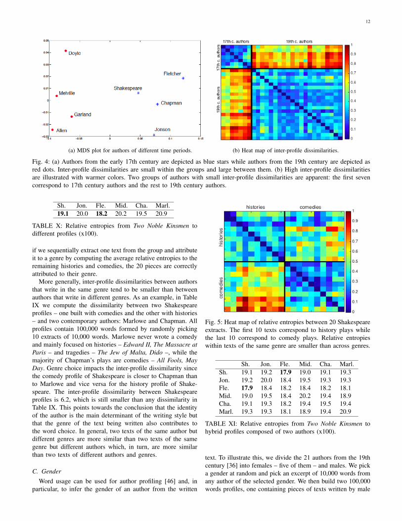
To further illustrate this point, in Fig. 4a we plot a twodimensional MDS representation of the dissimilarity betweeneight authors whose profiles were built with all their availabletexts in our corpus [36]. Four of the profiles correspond toearly 17th century authors – Shakespeare, Chapman, Jonson,and Fletcher – and are represented by blue stars while theother four – Doyle, Melville, Garland, and Allen – correspondto 19th century authors and are represented by red dots.Notice that authors tend to have a smaller distance with theircontemporaries and a larger distance with authors from otherperiods. This fact is also illustrated by the heat map of inter-profile dissimilarities in Fig. 4b where bluish colors representsmaller entropies. The first 7 rows and columns correspondto authors of the 17th century whereas the remaining 21correspond to authors of the 19th century, where profiles werebuilt with all the available texts. Notice that the blocks of bluecolor along the diagonal are in perfect correspondence with thetime period of the authors, verifying that WANs can be usedto determine the time in which a text was written. The averageentropies among authors of the 17th century and among thoseof the 19th century are 0.096 and 0.098 respectively, whereasthe average entropies between authors of different epochs is0.273. I.e., the relative entropy between authors of differentepochs almost triples that of authors belonging to the sametime period.

B. Genre

Even though function words by themselves do not carrycontent, WANs constructed from a text contain, rather sur-prisingly, information about its genre. We illustrate this factin Fig. 5, where we present the relative entropy between 20pieces of texts written by Shakespeare of length 20,000 words,where 10 of them are history plays – e.g., Richard II, KingJohn, Henry VIII – and 10 of them are comedies – e.g., TheTempest, Measure for Measure, The Merchant of Venice. Asin Fig. 4b, bluish colors in Fig. 5 represent smaller relativeentropies. Two blocks along the diagonal can be distinguishedthat coincide with the plays of the two different genres. Indeed,

12

(a) MDS plot for authors of different time periods. (b) Heat map of inter-profile dissimilarities.

Fig. 4: (a) Authors from the early 17th century are depicted as blue stars while authors from the 19th century are depicted asred dots. Inter-profile dissimilarities are small within the groups and large between them. (b) High inter-profile dissimilaritiesare illustrated with warmer colors. Two groups of authors with small inter-profile dissimilarities are apparent: the first sevencorrespond to 17th century authors and the rest to 19th century authors.

Sh. Jon. Fle. Mid. Cha. Marl.19.1 20.0 18.2 20.2 19.5 20.9

TABLE X: Relative entropies from Two Noble Kinsmen todifferent profiles (x100).

if we sequentially extract one text from the group and attributeit to a genre by computing the average relative entropies to theremaining histories and comedies, the 20 pieces are correctlyattributed to their genre.

More generally, inter-profile dissimilarities between authorsthat write in the same genre tend to be smaller than betweenauthors that write in different genres. As an example, in TableIX we compute the dissimilarity between two Shakespeareprofiles – one built with comedies and the other with histories– and two contemporary authors: Marlowe and Chapman. Allprofiles contain 100,000 words formed by randomly picking10 extracts of 10,000 words. Marlowe never wrote a comedyand mainly focused on histories – Edward II, The Massacre atParis – and tragedies – The Jew of Malta, Dido –, while themajority of Chapman’s plays are comedies – All Fools, MayDay. Genre choice impacts the inter-profile dissimilarity sincethe comedy profile of Shakespeare is closer to Chapman thanto Marlowe and vice versa for the history profile of Shake-speare. The inter-profile dissimilarity between Shakespeareprofiles is 6.2, which is still smaller than any dissimilarity inTable IX. This points towards the conclusion that the identityof the author is the main determinant of the writing style butthat the genre of the text being written also contributes tothe word choice. In general, two texts of the same author butdifferent genres are more similar than two texts of the samegenre but different authors which, in turn, are more similarthan two texts of different authors and genres.

C. Gender

Word usage can be used for author profiling [46] and, inparticular, to infer the gender of an author from the written

Fig. 5: Heat map of relative entropies between 20 Shakespeareextracts. The first 10 texts correspond to history plays whilethe last 10 correspond to comedy plays. Relative entropieswithin texts of the same genre are smaller than across genres.

Sh. Jon. Fle. Mid. Cha. Marl.Sh. 19.1 19.2 17.9 19.0 19.1 19.3Jon. 19.2 20.0 18.4 19.5 19.3 19.3Fle. 17.9 18.4 18.2 18.4 18.2 18.1Mid. 19.0 19.5 18.4 20.2 19.4 18.9Cha. 19.1 19.3 18.2 19.4 19.5 19.4Marl. 19.3 19.3 18.1 18.9 19.4 20.9

TABLE XI: Relative entropies from Two Noble Kinsmen tohybrid profiles composed of two authors (x100).

text. To illustrate this, we divide the 21 authors from the 19thcentury [36] into females – five of them – and males. We picka gender at random and pick an excerpt of 10,000 words fromany author of the selected gender. We then build two 100,000words profiles, one containing pieces of texts written by male

13

Nr. of authors N. Bayes 1-NN 3-NN DT-gdi DT-ce SVM WAN Voting2 2.6 3.5 5.2 12.2 12.2 2.7 1.6 0.94 6.0 9.2 12.4 25.3 25.5 6.8 4.6 3.36 8.1 11.7 15.2 31.9 32.2 7.9 5.3 3.88 9.6 15.4 19.2 36.4 37.2 11.1 6.7 5.2

10 10.8 16.7 21.4 42.1 42.1 11.5 8.3 6.0

TABLE XII: Error rates in % achieved by different methods for profiles of 100,000 words and texts of 10,000 words. TheWANs achieve the smallest error rate among the methods considered separately. Voting decreases the error even further bycombining the relational data of the WANs with the frequency data of other methods.

authors and the other by female authors. In order to avoidbias, we do not include any text of the author from whichthe text to attribute was chosen in the gender profiles. Wethen attribute the chosen text between the two gender profiles.After repeating this procedure 5,000 times, we obtain a meanaccuracy of 0.63. Although this accuracy is lower than state-of-the-art gender profiling methods [47], the difference withrandom attribution, i.e. accuracy of 0.5, validates the fact thatWANs carry gender information about the authors.

D. CollaborationsWANs can also be used for the attribution of texts written

collaboratively between two or more authors. Since collabora-tion was a common practice for playwrights in the early 17thcentury, we consider the attribution of Early Modern Englishplays [36]. For a given play, we compute its relative entropyto six contemporary authors – Shakespeare, Jonson, Fletcher,Middleton, Chapman, and Marlowe – by generating 50 randomprofiles for each author of length 80,000 words and averagingthe 50 entropies to obtain one representative number. We donot consider Peele in the analysis due to the short total lengthof available texts.

When two authors collaborate to write a play, the resultingword adjacency network is close to the profiles of both authors,even though these profiles are built with plays of their soleauthorship. As an example, consider the play Two NobleKinsmen which is an accepted collaboration between Fletcherand Shakespeare [48]. In Table X, we present the relativeentropies between the play and the six analyzed authors.Notice that the two minimum entropies correspond to thosewho collaborated in writing it.

Collaboration can be further confirmed by the constructionof hybrid profiles, i.e. profiles built containing 40,000 wordsof two different authors. Each entry in Table XI correspondsto the relative entropy from Two Noble Kinsmen to a hybridprofile composed by the authors in the row and column ofthat entry. Notice that the diagonal of Table XI correspondsto profiles of sole authors and, thus, coincides with Table X.The smallest relative entropy in Table XI is achieved by thehybrid profile composed by Fletcher and Shakespeare, whichis consistent with the accepted attribution of the play.

VII. COMPARISON AND COMBINATION WITH FREQUENCYBASED METHODS

Machine learning tools have been used to solve attributionproblems by relying on the frequency of appearance of func-tion words [49]. These methods consider the number of times

an author uses different function words but, unlike WANs,do not contemplate the order in which the function wordsappear. The most common techniques include naive Bayes [50,Chapter 8], nearest neighbors (NN) [50, Chapter 2], decisiontrees (DT) [50, Chapter 14], and support vector machines(SVM) [50, Chapter 7].

In Table XII we inform the percentage of errors obtainedby different methods when attributing texts of 10,000 wordsamong profiles of 100,000 words for a number of authorsranging from two to ten. For a given number of candidateauthors, we randomly pick them from the pool of 19th centuryauthors [36] and attribute ten excerpts of each of them usingthe different methods. We then repeat the random choice ofauthors 100 times and average the error rate. For each ofthe methods based on function word frequencies, we pickthe set of parameters and preprocessing that minimize theattribution error rate. E.g., for SVM the error is minimizedwhen considering a polynomial kernel of degree 3 and normal-izing the frequencies by text length. For the nearest neighborsmethod we consider two strategies based on one (1-NN) andthree (3-NN) nearest neighbors as given by the l2 metric inEuclidean space. Also, for decision trees we consider twotypes of split criteria: the Gini Diversity Index (DT-gdi) andthe cross-entropy (DT-ce) [51].

The WANs achieve a lower attribution error than frequencybased methods; see Table XII. For binary attributions, naiveBayes and SVM achieve error rates of 2.6% and 2.7% respec-tively and, thus, outperform nearest neighbors and decisiontrees. However, WANs outperform the aforementioned meth-ods by obtaining an error rate of 1.6%. This implies a reductionof 38% in the error rate. For 6 authors, WANs achieve an errorrate of 5.3% that outperform SVMs achieving 7.9% entailing a33% reduction. This trend is consistent across different numberof candidate authors, with WANs achieving an average errorreduction of 29% compared with the best traditional machinelearning method.

More important than the fact that WANs tend to outperformmethods based on word frequencies, is the fact that they carrydifferent stylometric information. Thus, we can combine bothmethodologies to further increase attribution accuracy. We dothis via a voting method, where we perform majority votingbetween WANs and the two best performing frequency basedmethods, namely, naive Bayes and SVMs. More specifically,each of the three methods gives one vote to its preferred candi-date author and then the voting method chooses the author withmore votes. In case of a three-way tie, the candidate author

14

voted by the WANs is chosen. In the last column of TableXII we inform the error rate of majority voting. These errorrates are consistently smaller than those achieved by WANsand, hence, by the other frequency based methods as well.E.g., for attributions among four authors, voting achieves anerror of 3.3% compared to an error of 4.6% of WANs. Thiscorresponds to a 28% reduction in error. Averaging amongattributions for different number of candidate authors, majorityvoting entails a reduction of 30% compared with WANs. Thecombination of WANs and function word frequencies halvesthe attribution error rate with respect to the traditional machinelearning methods.

Although the error rates presented in Table XII correspondto profiles of balanced length, the results also hold for sce-narios where different profiles contain different number ofwords. This means that, for unbalanced scenarios, the WANsstill outperform traditional classifiers and the voting methodalso achieves the lowest error rates.

VIII. CONCLUSIONS AND FUTURE WORK

Relational data between function words was used as stylo-metric information to solve authorship attribution problems.Normalized word adjacency networks (WANs) were used asrelational structures. We interpreted these networks as Markovchains in order to facilitate their comparison using relativeentropies. The accuracy of WANs was analyzed for varyingnumber of candidate authors, text lengths, profile lengths anddifferent levels of heterogeneity among the candidate authors,regarding genre, gender, and time period. The method worksbest when the corpora of known texts is of substantial length,when the texts being attributed are long, or when the numberof candidate authors is small. If long profiles are available– more than 60,000 words, corresponding to 150 pages ofa midsize paperback book –, we demonstrated very highattribution accuracy for texts longer than a few typical novelchapters even when attributing between a large number ofauthors, high accuracy for texts as long as a play act or a novelchapter, and reasonable rates for short texts such as newspaperopinion pieces if the number of candidate authors is small.WANs were also shown to classify accurately the time periodwhen a text was written, to acceptably estimate the genre ofa piece, and to have some predictive power on the genderof the author. The applicability of WANs to identify multipleauthors in collaborative works was also demonstrated. Withregards to existing methods based on the frequency with whichdifferent function words appear in the text, we observed thatWANs exceed their classification accuracy. More importantly,we showed that WANs and frequencies captured differentstylometric aspects so that their combination is possible andends up halving the error rate of existing methods.

As directions for future research, we plan to investigatemore sophisticated ways to combine the attribution powerof WANs with existing methods in order to improve theattribution accuracy in general and to gain discriminatingpower for short texts. Moreover, we want to extend our methodtowards the attribution of other types of creative work such asthe identification of a composer based on a musical piece.

REFERENCES

[1] S. Segarra, M. Eisen, and A. Ribeiro, “Authorship attribution usingfunction words adjacency networks,” in Acoustics, Speech and SignalProcessing (ICASSP), 2013 IEEE International Conference on, 2013,pp. 5563–5567.

[2] T. Grant, “Quantifying evidence in forensic authorship analysis,” Inter-national Journal of Speech Language and the Law, vol. 14, no. 1, 2007.

[3] A. Abbasi and H. Chen, “Applying authorship analysis to extremist-group web forum messages,” Intelligent Systems, IEEE, vol. 20, no. 5,pp. 67–75, Sept 2005.

[4] S. Meyer zu Eissen, B. Stein, and M. Kulig, “Plagiarism detectionwithout reference collections,” in Advances in Data Analysis, ser.Studies in Classification, Data Analysis, and Knowledge Organization,R. Decker and H.-J. Lenz, Eds. Springer Berlin Heidelberg, 2007, pp.359–366.

[5] D. I. Holmes, “Authorship attribution,” Computers and the Humanities,vol. 28, no. 2, pp. 87–106, 1994.

[6] P. Juola, “Authorship attribution,” Foundations and Trends in Informa-tion Retrieval, vol. 1, pp. 233–334, 2006.

[7] E. Stamatatos, “A survey of modern authorship attribution methods,”Journal of the American Society for Information Science and Technol-ogy, vol. 60, pp. 538–556, March 2009.

[8] T. C. Mendenhall, “The characteristic curves of composition,” Science,vol. 9, pp. 237–246, 1887.

[9] G. U. Yule, “On sentence-length as a statistical characteristic of style inprose: With application to two cases of disputed authorship,” Biometrika,vol. 30, pp. 363–390, 1939.

[10] F. Mosteller and D. Wallace, “Inference and disputed authorship: Thefederalist,” Addison-Wesley, 1964.

[11] J. F. Burrows, “an ocean where each kind...: Statistical analysis and somemajor determinants of literary style,” Computers and the Humanities,vol. 23, pp. 309–321, 1989.

[12] D. I. Holmes and R. S. Forsyth, “The federalist revisited: New directionsin authorship attribution,” Literary and Linguistic Computing, vol. 10,pp. 111–127, 1995.

[13] D. L. Hoover, “Delta prime?” Literary and Linguistic Computing,vol. 19, no. 4, pp. 477–495, 2004.

[14] H. van Halteren, R. H. Baayen, F. Tweedie, M. Haverkort, and A. Neijt,“New machine learning methods demonstrate the existence of a humanstylome,” Journal of Quantitative Linguistics, vol. 12, no. 1, pp. 65–77,2005.

[15] B. Yu, “Function words for chinese authorship attribution,” in Proceed-ings of the NAACL-HLT 2012 Workshop on Computational Linguisticsfor Literature. Association for Computational Linguistics, 2012, pp.45–53.

[16] M. Ebrahimpour, T. J. Putnins, M. J. Berryman, A. Allison, B. W.-H. Ng,and D. Abbott, “Automated authorship attribution using advanced signalclassification techniques,” PloS one, vol. 8, no. 2, p. e54998, 2013.

[17] R. S. Forsyth and D. I. Holmes, “Feature-finding for test classification,”Literary and Linguistic Computing, vol. 11, pp. 163–174, 1996.

[18] G. U. Yule, “The statistical study of literary vocabulary,” CUP Archive,1944.

[19] D. I. Holmes, “Vocabulary richness and the prophetic voice,” Literaryand Linguistic Computing, vol. 6, pp. 259–268, 1991.

[20] F. J. Tweedie and R. H. Baayen., “How variable may a constantbe? measures of lexical richness in perspective,” Computers and theHumanities, vol. 32, pp. 323–352, 1998.

[21] D. Hoover, “Another perspective on vocabulary richness,” Computersand the Humanities, vol. 37, pp. 151–178, 2003.

[22] M. Koppel, N. Akiva, and I. Dagan, “Feature instability as a criterion forselecting potential style markers,” Journal of the American Society forInformation Science and Technology, vol. 57, pp. 1519–1525, September2006.

[23] D. Cutting, J. Kupiec, J. Pedersen, and P. Sibun, “A practical part-of-speech tagger,” Proceedings of the third conference on Applied NaturalLanguage Processing, pp. 133–140, 1992.

[24] T. Solorio, S. Pillay, S. Raghavan, and M. Montes-y Gomez, “Modalityspecific meta features for authorship attribution in web forum posts.” inIJCNLP, 2011, pp. 156–164.

[25] G. Sidorov, F. Velasquez, E. Stamatatos, A. Gelbukh, and L. Chanona-Hernandez, “Syntactic n-grams as machine learning features for naturallanguage processing,” Expert Systems with Applications, vol. 41, no. 3,pp. 853–860, 2014.

15

[26] Y. Seroussi, I. Zukerman, and F. Bohnert, “Authorship attribution withlatent dirichlet allocation,” in Proceedings of the fifteenth conference oncomputational natural language learning. Association for Computa-tional Linguistics, 2011, pp. 181–189.

[27] L. Pearl and M. Steyvers, “Detecting authorship deception: a supervisedmachine learning approach using author writeprints,” Literary andlinguistic computing, p. fqs003, 2012.

[28] J. Savoy, “Authorship attribution based on a probabilistic topic model,”Information Processing & Management, vol. 49, no. 1, pp. 341–354,2013.

[29] D. V. Khmelev and F. Tweedie, “Using markov chains for identificationof writers,” Literary and linguistic computing, vol. 16, pp. 299–307,2001.

[30] O. V. Kukushkina, A. A. Polikarpov, and D. V. Khmelev, “Usingliteral and grammatical statistics for authorship attribution,” Problemsof Information Transmission, vol. 37, pp. 172–184, 2001.

[31] C. Sanderson and S. Guenter, “Short text authorship attribution via se-quence kernels, markov chains and author unmasking: An investigation,”in Proceedings of the 2006 Conference on Empirical Methods in NaturalLanguage Processing. Association for Computational Linguistics, 2006,pp. 482–491.

[32] M. J. Collins, “A new statistical parser based on bigram lexical depen-dencies,” in Proceedings of the 34th annual meeting on Association forComputational Linguistics. Association for Computational Linguistics,1996, pp. 184–191.

[33] H. Lodhi, C. Saunders, J. Shawe-Taylor, N. Cristianini, and C. Watkins,“Text classification using string kernels,” The Journal of MachineLearning Research, vol. 2, pp. 419–444, 2002.

[34] C. Cortes, P. Haffner, and M. Mohri, “A machine learning frameworkfor spoken-dialog classification,” in Springer Handbook of Speech Pro-cessing. Springer, 2008, pp. 585–596.

[35] R. Quirk, S. Greenbaum, G. Leech, and J. Svartvik, “A comprehensivegrammar of the english language,” Longman, 1985.

[36] S. Segarra, M. Eisen, and A. Ribeiro, “Compilation of texts used forthe numerical experiments (journal materials),” https://fling.seas.upenn.edu/∼maeisen/wiki/ index.php?n=Main.TextAttribution2, 2014.

[37] G. Kesidis and J. Walrand, “Relative entropy between markov transitionrate matrices,” IEEE Trans. Information Theory, vol. 39, pp. 1056–1057,May 1993.

[38] Z. Rached, F. Alajaji, and L. Campbell, “The kullback-leibler divergencerate between markov sources,” Information Theory, IEEE Transactionson, vol. 50, no. 5, pp. 917–921, May 2004.

[39] H. Tang, M. Hasegawa-Johnson, and T. Huang, “Non-frontal view facialexpression recognition based on ergodic hidden markov model super-vectors,” in Multimedia and Expo (ICME), 2010 IEEE InternationalConference on, July 2010, pp. 1202–1207.

[40] M. Vidyasagar, S. Mande, C. Reddy, and V. Rao, “The 4m (mixedmemory markov model) algorithm for finding genes in prokaryoticgenomes,” Automatic Control, IEEE Transactions on, vol. 53, no. SpecialIssue, pp. 26–37, Jan 2008.

[41] Y. Zhao, J. Zobel, and P. Vines, “Using relative entropy for authorshipattribution,” in Information Retrieval Technology, ser. Lecture Notes inComputer Science, H. Ng, M.-K. Leong, M.-Y. Kan, and D. Ji, Eds.Springer Berlin Heidelberg, 2006, vol. 4182, pp. 92–105.

[42] R. Arun, V. Suresh, and C. V. Madhavan, “Stopword graphs andauthorship attribution in text corpora,” in Semantic Computing, 2009.ICSC’09. IEEE International Conference on. IEEE, 2009, pp. 192–196.

[43] C. D. Manning, P. Raghavan, and H. Schutze, Introduction to Infor-mation Retrieval. New York, NY, USA: Cambridge University Press,2008.

[44] T. W. Anderson and L. A. Goodman, “Statistical inference about markovchains,” The Annals of Mathematical Statistics, pp. 89–110, 1957.

[45] M. A. A. Cox and T. F. Cox, “Multidimensional scaling,” in Handbook ofData Visualization, ser. Springer Handbooks Comp.Statistics. SpringerBerlin Heidelberg, 2008, pp. 315–347.

[46] S. Argamon, M. Koppel, J. W. Pennebaker, and J. Schler, “Automaticallyprofiling the author of an anonymous text,” Commun. ACM, vol. 52,no. 2, pp. 119–123, Feb. 2009.

[47] M. Koppel, S. Argamon, and A. R. Shimoni, “Automatically categorizingwritten texts by author gender,” Literary and Linguistic Computing,vol. 17, no. 4, pp. 401–412, 2002.

[48] E. A. B. Farmer and Z. Lesser, “Deep: Database of Early EnglishPlaybooks,” http://deep.sas.upenn.edu/ , 2007. [Online]. Available:http://deep.sas.upenn.edu/

[49] Y. Zhao and J. Zobel, “Effective and scalable authorship attribution usingfunction words,” in Information Retrieval Technology, ser. Lecture Notesin Computer Science, G. Lee, A. Yamada, H. Meng, and S. Myaeng,Eds. Springer Berlin Heidelberg, 2005, vol. 3689, pp. 174–189.

[50] C. M. Bishop, Pattern Recognition and Machine Learning (InformationScience and Statistics). Secaucus, NJ, USA: Springer-Verlag New York,Inc., 2006.

[51] L. Breiman, J. Friedman, C. J. Stone, and R. A. Olshen, Classificationand regression trees. CRC press, 1984.

https://fling.seas.upenn.edu/~maeisen/wiki/index.php?n=Main.TextAttribution2

https://fling.seas.upenn.edu/~maeisen/wiki/index.php?n=Main.TextAttribution2

http://deep.sas.upenn.edu/

http://deep.sas.upenn.edu/

authorship attribution through function word adjacency...

Documents