auto-keras: efficient neural architecture search … efficient neural architecture search with...
TRANSCRIPT
AUTO-KERAS: EFFICIENT NEURAL ARCHITECTURE SEARCH WITHNETWORK MORPHISM
Haifeng Jin 1 Qingquan Song 1 Xia Hu 1
ABSTRACTNeural architecture search (NAS) has been proposed to automatically tune deep neural networks, but existingsearch algorithms usually suffer from expensive computational cost. Network morphism, which keeps thefunctionality of a neural network while changing its neural architecture, could be helpful for NAS by enablinga more efficient training during the search. In this paper, we propose a novel framework enabling Bayesianoptimization to guide the network morphism for efficient neural architecture search by introducing a neuralnetwork kernel and a tree-structured acquisition function optimization algorithm, which more efficiently exploresthe search space. Intensive experiments have been done to demonstrate the superior performance of the developedframework over the state-of-the-art methods. Moreover, we build an open-source AutoML system on our method,namely Auto-Keras2. The system runs in parallel on CPU and GPU, with an adaptive search strategy for differentGPU memory limits.
1 INTRODUCTION
Automated Machine Learning (AutoML) has become a veryimportant research topic with the wide application of ma-chine learning techniques. The goal of AutoML is to enablepeople with limited machine learning background knowl-edge to use the machine learning models easily. In thecontext of deep learning, neural architecture search (NAS),which aims to search for the best neural network architec-ture for the given learning task and dataset, has becomean effective computational tool in AutoML. Unfortunately,existing NAS algorithms are usually computationally expen-sive. The time complexity of NAS can be seen as O(nt),where n is the number of neural architectures evaluatedduring the search, and t is the average time consumptionfor evaluating each of the n neural networks. Many NASapproaches, such as deep reinforcement learning (Zoph &Le, 2016; Baker et al., 2016; Zhong et al., 2017; Pham et al.,2018) and evolutionary algorithms (Real et al., 2017; Desell,2017; Liu et al., 2017; Suganuma et al., 2017; Xie & Yuille,2017; Real et al., 2018), require a large n to reach a goodperformance. Also, each of the n neural networks is trainedfrom scratch which is very slow.
Network morphism has also been explored for neural archi-tecture search (Cai et al., 2018; Elsken et al., 2017). Net-work morphism is a technique to morph the architecture of aneural network but keep its functionality (Chen et al., 2015;Wei et al., 2016). Therefore, we are able to modify a trained
1 Department of Computer Science and Engineering, TexasA&M University, College Station, United States.
2 The code is available at http://autokeras.com.
neural network into a new architecture using the networkmorphism operations, e.g., inserting a layer or adding a skip-connection. Only a few more epochs are required to furthertrain the new architecture for better performance. Usingnetwork morphism would reduce the average training timet in neural architecture search. The most important problemto solve for network morphism based NAS methods is theselection of operations, which is to select from the networkmorphism operation set to morph an existing architectureto a new one. The state-of-the-art network morphism basedmethod (Cai et al., 2018) uses a deep reinforcement learningcontroller, which requires a large number of training exam-ples, i.e., n in O(nt). Another simple approach (Elskenet al., 2017) is to use random algorithm and hill-climbing,which can only explore the neighborhoods of the searchedarea each time, and could potentially be trapped by local op-timum. How to perform efficient neural architecture searchwith network morphism remains a challenging problem.
As we know, Bayesian optimization (Snoek et al., 2012)has been widely adopted to efficiently explore black-boxfunctions for global optimization, whose observations areexpensive to obtain. For example, it has been used in hyper-parameter tuning for machine learning models (Thorntonet al., 2013; Kotthoff et al., 2016; Feurer et al., 2015; Hut-ter et al., 2011), in which Bayesian optimization searchesamong different combinations of hyperparameters. Duringthe search, each evaluation of a combination of hyperparam-eters involves an expensive process of training and testingof the machine learning model, which is very similar tothe NAS problem. The unique properties of Bayesian opti-
arX
iv:1
806.
1028
2v2
[cs
.LG
] 3
Oct
201
8
Auto-Keras: Efficient Neural Architecture Search with Network Morphism
mization motivate us to explore its capability in guiding thenetwork morphism to reduce the number of trained neuralnetworks n to make the search more efficient.
It is a non-trivial task to design a Bayesian optimizationmethod for network morphism based neural architecturesearch due to the following challenges. First, the underlyingGaussian process (GP) is traditionally used for Euclideanspace. To update the Bayesian optimization model withobservations, the underlying GP is to be trained with thesearched architectures and their performance. However, theneural network architectures are not in Euclidean space andhard to parameterize into a fixed-length vector. Second,an acquisition function needs to be optimized for Bayesianoptimization to generate the next architecture to observe.However, it is not to maximize a function in Euclidean spacefor morphing the neural architectures, but to select a node toexpand in a tree-structured search space, where each noderepresents an architecture and each edge a morph operation.Thus traditional Newton-like or gradient-based methodscannot be simply applied. Third, the network morphismoperations are complicated in a search space of neural ar-chitectures with skip-connections. A network morphismoperation on one layer may change the shapes of some inter-mediate output tensors, which no longer match input shaperequirements of the layers taking them as input. How tomaintain such consistency is not defined in previous workon network morphism.
In this paper, an efficient neural architecture search withnetwork morphism is proposed, which utilizes Bayesianoptimization to guide through the search space by select-ing the most promising operations each time. To tackle theaforementioned challenges, an edit-distance based neuralnetwork kernel is constructed. Being consistent with thekey idea of network morphism, it measures how many oper-ations are needed to change one neural network to another.Besides, a novel acquisition function optimizer, which is ca-pable of balancing between the exploration and exploitation,is designed specially for the tree-structure search space toenable Bayesian optimization to select from the operations.In addition, a graph-level morphism is defined to address thecomplicated changes in the neural architectures based onprevious layer-level network morphism. The proposed ap-proach is compared with the state-of-the-art NAS methods(Kandasamy et al., 2018; Elsken et al., 2017) on bench-mark datasets of MNIST, CIFAR10, and FASHION-MNIST.Within a limited search time, the architectures found by ourmethod achieves the lowest error rates on all of the datasets.
In addition, we develop an open-source AutoML systembased on our proposed method, namely Auto-Keras, whichcan be download and installed locally. The system is care-fully designed with a concise interface for people not spe-cialized in computer programming and data science to use.
To speed up the search, the workload on CPU and GPUcan run in parallel. To address the issue of different GPUmemory, which limits the size of the neural architectures, amemory adaption strategy is designed for deployment.
The main contributions of the paper are as follows:
• An algorithm for efficient neural architecture searchwith Bayesian optimization guided network morphismis proposed.
• Propose a neural network kernel for Bayesian optimiza-tion, a tree-structured acquisition function optimizer,and a graph-level morphism.
• Conduct intensive experiments on benchmark datasetsto demonstrate the superior performance of the pro-posed method over the baseline methods.
• An open-source AutoML system, namely Auto-Keras,is developed based on our method for neural architec-ture search.
2 PROBLEM STATEMENT
The general neural architecture search problem we studiedin this paper is defined as: given a neural architecture searchspace F , the input dataX , and the cost metric Cost(·), weaim at finding an optimal neural network f∗ ∈ F with itstrained parameter θf∗ , which could achieve the lowest costmetric value on the given datasetX . Mathematically, thisdefinition is equivalent to finding f∗ satisfing:
f∗ = argminf∈F
minθf
Cost(f(X;θf )), (1)
where θf ∈ Rw(f) denotes the parameter set of network f ,w(f) is the number of parameters in f .
Before explaining the proposed algorithm, we first definethe target search space F . Let Gf = (Vf , Ef ) denotesthe computational graph of a neural network f . Each nodev ∈ Vf denotes an intermediate output tensor of a layer of f .Each directed edge eu→v ∈ Ef denotes a layer of f , whoseinput tensor is u ∈ Vf and output tensor is v ∈ Vf . u ≺ vindicates v is before u in topological order of the nodes,i.e., by traveling through the edges in Ef , u is reachablefrom node v. The search space F in this work is definedas: a space consisting of any neural network architecture f ,which satisfies two conditions: (1) Gf is a directed acyclicgraph (DAG). (2) ∀u v ∈ Vf , (u ≺ v)∨(v ≺ u). It is worthpointing out that although skip connection is allowed, thereshould only be one main chain in f . Moreover, the searchspace F defined here is large enough to cover a wide rangeof famous neural architectures, e.g., DenseNet, ResNet.
Auto-Keras: Efficient Neural Architecture Search with Network Morphism
3 NETWORK MORPHISM WITH BAYESIANOPTIMIZATION
The key idea of the proposed method is to explore the searchspace via morphing the network architectures guided byan efficient Bayesian optimization algorithm. TraditionalBayesian optimization consists of a loop of three steps: up-date, generation, and observation. In the context of NAS, ourproposed Bayesian optimization algorithm iteratively con-ducts: (1) Update: train the underlying Gaussian processmodel with the existing architectures and their performance;(2) Generation: generate the next architecture to observeby optimizing an delicately defined acquisition function; (3)Observation: train the generated neural architecture to ob-tain the actual performance. There are three main challengesin designing the method for morphing the neural architec-tures with Bayesian optimization. We introduce three keycomponents separately in the subsequent sections copingwith the three design challenges.
3.1 Neural Network Kernel for Gaussian Process
The first challenge we need to address is that the NAS spaceis not a Euclidean space, which does not satisfy the assump-tion of the traditional Gaussian process. Directly vectorizingthe neural architecture is impractical due to the uncertainnumber of layers and parameters it may contain. Since theGaussian process is a kernel method, instead of vectorizinga neural architecture, we propose to tackle the challenge bydesigning a neural network kernel function. The intuitionbehind the kernel function is the edit-distance for morphingone neural architecture to another.
Kernel Definition: Suppose fa and fb are two neural net-works. Inspired by Deep Graph Kernels (Yanardag & Vish-wanathan, 2015), we propose an edit-distance kernel forneural networks, which accords with our idea of employingnetwork morphism. Edit-distance here means how many op-erations are needed to morph one neural network to another.The concrete kernel function is defined as follows:
κ(fa, fb) = e−ρ2(d(fa,fb)), (2)
where function d(·, ·) denotes the edit-distance of two neuralnetworks, whose range is [0,+∞), ρ is a mapping function,which maps the distance in the original metric space to thecorresponding distance in the new space. The new spaceis constructed by embedding the original metric space intoa new one using Bourgain Theorem (Bourgain, 1985), thepurpose of which is to ensure the validity of the kernel.More details are introduced in Theorem 2.
Calculating the edit-distance of two neural networks canbe mapped to calculating the edit-distance of two graphs,which is an NP-hard problem (Zeng et al., 2009). Basedon the search space F we have defined in Section 2, we
solve the problem by proposing an approximated solutionas follows:
d(fa, fb) = Dl(La, Lb) + λDs(Sa, Sb), (3)
where Dl denotes the edit-distance for morphing the lay-ers, i.e., the minimum edit needed to morph fa to fb ifthe skip-connections are ignored, La = l(1)a , l
(2)a , . . .
and Lb = l(1)b , l(2)b , . . . are the layer sets of neural net-
works fa and fb, Ds is the approximated edit-distance formorphing skip-connections between two neural networks,Sa = s(1)a , s
(2)a , . . . and Sb = s(1)b , s
(2)b , . . . are the
skip-connection sets of neural network fa and fb, and λ isthe balancing factor.
Calculating Dl: We assume |La| < |Lb|, the edit-distancefor morphing the layers of two neural architectures fa andfb is calculated by minimizing the follow equation:
Dl(La, Lb) = min
|La|∑i=1
dl(l(i)a , ϕl(l
(i)a )) +
∣∣∣|Lb| − |La|∣∣∣,(4)
where ϕl : La → Lb is an injective matching function oflayers satisfying: ∀i < j, ϕl(l
(i)a ) ≺ ϕl(l(j)a ) if layers in La
and Lb are all sorted in topological order. dl(·, ·) denotesthe edit-distance of widening a layer into another defined inEquation (5), where w(l) is the width of layer l.
dl(la, lb) =|w(la)− w(lb)|max[w(la), w(lb)]
. (5)
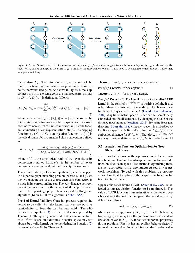
The intuition of Equation (4) is consistent with the idea ofnetwork morphism shown in Figure 1. Suppose a matchingis provided between the nodes in two neural networks. Thesize of the tensors are indicators of the width of the previouslayers (e.g., the output vector length of a fully-connectedlayer or the number of filters of a convolutional layer). Thematchings between the nodes are marked by light blue. Soa matching between the nodes can be seen as a matchingbetween the layers. To morph fa to fb with the given match-ing, we need to first widen the three nodes in fa to the samewidth as their matched nodes in fb, and then insert a newnode of width 20 after the first node in fa. Based on thismorphing scheme, the overall edit-distance of the layers isdefined as Dl in Equation (4).
Since there are many ways to morph fa to fb, to find the bestmatching between the nodes that minimizes Dl, we proposea dynamic programming approach by defining a matrixA|La|×|Lb|, which is recursively calculated as follows:
Ai,j = max[Ai−1,j+1,Ai,j−1+1,Ai−1,j−1+dl(l(i)a , l
(j)b )],(6)
where Ai,j is the minimum value of Dl(L(i)a , L
(j)b ),
where L(i)a = l(1)a , l
(2)a , . . . , l
(i)a and L
(j)b =
l(1)b , l(2)b , . . . , l
(j)b .
Auto-Keras: Efficient Neural Architecture Search with Network Morphism
Figure 1. Neural Network Kernel. Given two neural networks fa, fb, and matchings between the similar layers, the figure shows how thelayers of fa can be changed to the same as fb. Similarly, the skip-connections in fa also need to be changed to the same as fb accordingto a given matching.
Calculating Ds: The intuition of Ds is the sum of thethe edit-distances of the matched skip-connections in twoneural networks into pairs. As shown in Figure 1, the skip-connections with the same color are matched pairs. Similarto Dl(·, ·), Ds(·, ·) is defined as follows:
Ds(Sa, Sb) = min
|Sa|∑i=1
ds(s(i)a , ϕs(s
(i)a )) +
∣∣∣|Sb| − |Sa|∣∣∣,(7)
where we assume |Sa| < |Sb|. (|Sb| − |Sa|) measures thetotal edit-distance for non-matched skip-connections sinceeach of the non-matched skip-connections in Sb calls for anedit of inserting a new skip connection into fa. The mappingfunction ϕs : Sa → Sb is an injective function. ds(·, ·) isthe edit-distance for two matched skip-connections definedas:
ds(sa, sb) =|u(sa)− u(sb)|+ |δ(sa)− δ(sb)|
max[u(sa), u(sb)] +max[δ(sa), δ(sb)],
(8)where u(s) is the topological rank of the layer the skip-connection s started from, δ(s) is the number of layersbetween the start and end point of the skip-connection s.
This minimization problem in Equation (7) can be mappedto a bipartite graph matching problem, where fa and fb arethe two disjoint sets of the graph, each skip-connection isa node in its corresponding set. The edit-distance betweentwo skip-connections is the weight of the edge betweenthem. The bipartite graph problem is solved by Hungarianalgorithm (Kuhn-Munkres algorithm) (Kuhn, 1955).
Proof of Kernel Validity: Gaussian process requires thekernel to be valid, i.e., the kernel matrices are positivesemidefinite, to keep the distributions valid. The edit-distance in Equation (3) is a metric distance proved byTheorem 1. Though, a generalized RBF kernel in the formof e−γd(x,y) based on a distance in metric space may notalways be a valid kernel, our kernel defined in Equation (2)is proved to be valid by Theorem 2.
Theorem 1. d(fa, fb) is a metric space distance.
Proof of Theorem 1: See appendix.
Theorem 2. κ(fa, fb) is a valid kernel.
Proof of Theorem 2: The kernel matrix of generalized RBFkernel in the form of e−γD
2(x,y) is positive definite if andonly if there is an isometric embedding in Euclidean spacefor the metric space with metric D (Haasdonk & Bahlmann,2004). Any finite metric space distance can be isometricallyembedded into Euclidean space by changing the scale of thedistance measurement (Maehara, 2013). By using Bourgaintheorem (Bourgain, 1985), metric space d is embedded toEuclidean space with little distortion. ρ(d(fa, fb)) is theembedded distance for d(fa, fb). Therefore, e−ρ
2(d(fa,fb))
is always positive definite. So κ(fa, fb) is a valid kernel.
3.2 Acquisition Function Optimization for TreeStructured Space
The second challenge is the optimization of the acquisi-tion function. The traditional acquisition functions are de-fined on Euclidean space. The methods optimizing themare not applicable to the tree-structured search via net-work morphism. To deal with this problem, we proposea novel method to optimize the acquisition function fortree-structured space.
Upper-confidence bound (UCB) (Auer et al., 2002) is se-lected as our acquisition function to be minimized. Thevalue of UCB function is an estimation of the lowest pos-sible value of the cost function given the neural network fdefined as follows
α(f) = µ(yf )− βσ(yf ), (9)
where yf = minθf Cost(f(X;θf )), β is the balancingfactor, µ(yf ) and σ(yf ) are the posterior mean and standarddeviation of variable yf . UCB has two important propertiesfit our problem. First, it has an explicit balance factor βfor exploration and exploitation. Second, the function value
Auto-Keras: Efficient Neural Architecture Search with Network Morphism
is directly comparable with the cost function value c(i) insearch historyH = (f (i),θ(i), c(i)). With the acquisitionfunction, f = argminfα(f) is the generated architecturefor next observation.
The tree-structured space is defined as follows. Duringthe optimization of the α(f), f should be obtained fromf (i) and O, where f (i) is an observed architecture in thesearch history H, O is a sequence of operations to morphthe architecture into a new one. Morph f to f with O isdenoted as f ←M(f,O), whereM(·, ·) is the function tomorph f with the operations in O. Therefore, the searchcan be viewed as a tree-structured search, where each nodeis a neural architecture, whose children are morphed from itby network morphism operations.
The most common defect of network morphism is it onlygrows the size of the architecture instead of shrinking them.Some other work using network morphism for NAS (Elskenet al., 2018) would end up with a very large architecturewithout enough exploration on the smaller architectures.The main reason is they only morph the current best archi-tectures instead of the smaller architectures found earlier inthe search. However, in our tree-structure search, we cannot only expand the leaves but also the inner nodes, whichmeans the smaller architectures found in the early stage canbe selected multiple times to morph to more architectures.
The state-of-the-art acquisition function optimization tech-niques, e.g., gradient-based or Newton-like method, aredesigned for numerical data, which do not apply in thetree-structure space. TreeBO (Jenatton et al., 2017) hasproposed a way to maximize the acquisition function ina tree-structured parameter space. However, only the leafnodes of its tree have acquisition function values, which isdifferent from our case. Moreover, the proposed solution isa surrogate multivariate Bayesian optimization model. InNASBOT (Kandasamy et al., 2018), they use an evolution-ary algorithm to optimize the acquisition function. They areboth very expansive in computing time. To optimize our ac-quisition function, we need a method to efficiently optimizethe acquisition function in the tree-structured space.
Inspired by the various heuristic search algorithms for ex-ploring the tree-structured search space and optimizationmethods balancing between exploration and exploitation,a new method based on A* search and simulated anneal-ing is proposed. A* is for tree-structure search. Simulatedannealing is for balancing exploration and exploitation.
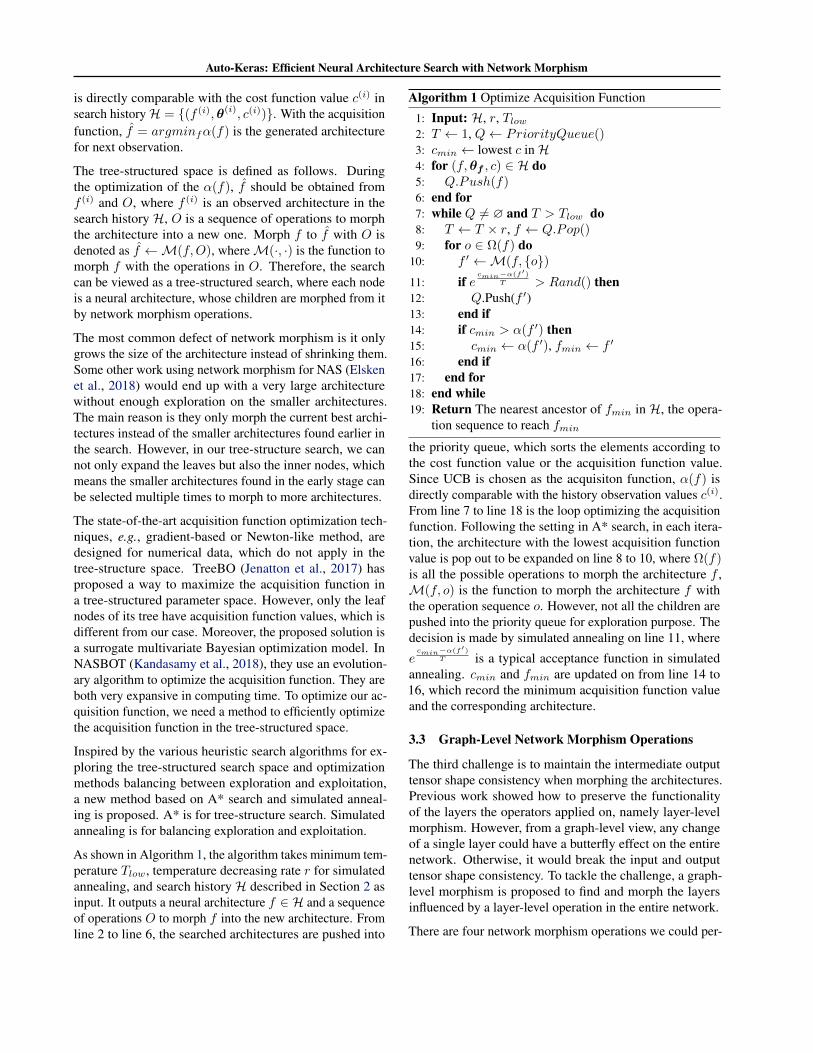
As shown in Algorithm 1, the algorithm takes minimum tem-perature Tlow, temperature decreasing rate r for simulatedannealing, and search history H described in Section 2 asinput. It outputs a neural architecture f ∈ H and a sequenceof operations O to morph f into the new architecture. Fromline 2 to line 6, the searched architectures are pushed into
Algorithm 1 Optimize Acquisition Function
1: Input: H, r, Tlow2: T ← 1, Q← PriorityQueue()3: cmin ← lowest c inH4: for (f,θf , c) ∈ H do5: Q.Push(f)6: end for7: while Q 6= ∅ and T > Tlow do8: T ← T × r, f ← Q.Pop()9: for o ∈ Ω(f) do
10: f ′ ←M(f, o)11: if e
cmin−α(f′)T > Rand() then
12: Q.Push(f ′)13: end if14: if cmin > α(f ′) then15: cmin ← α(f ′), fmin ← f ′
16: end if17: end for18: end while19: Return The nearest ancestor of fmin in H, the opera-
tion sequence to reach fmin
the priority queue, which sorts the elements according tothe cost function value or the acquisition function value.Since UCB is chosen as the acquisiton function, α(f) isdirectly comparable with the history observation values c(i).From line 7 to line 18 is the loop optimizing the acquisitionfunction. Following the setting in A* search, in each itera-tion, the architecture with the lowest acquisition functionvalue is pop out to be expanded on line 8 to 10, where Ω(f)is all the possible operations to morph the architecture f ,M(f, o) is the function to morph the architecture f withthe operation sequence o. However, not all the children arepushed into the priority queue for exploration purpose. Thedecision is made by simulated annealing on line 11, where
ecmin−α(f′)
T is a typical acceptance function in simulatedannealing. cmin and fmin are updated on from line 14 to16, which record the minimum acquisition function valueand the corresponding architecture.
3.3 Graph-Level Network Morphism Operations
The third challenge is to maintain the intermediate outputtensor shape consistency when morphing the architectures.Previous work showed how to preserve the functionalityof the layers the operators applied on, namely layer-levelmorphism. However, from a graph-level view, any changeof a single layer could have a butterfly effect on the entirenetwork. Otherwise, it would break the input and outputtensor shape consistency. To tackle the challenge, a graph-level morphism is proposed to find and morph the layersinfluenced by a layer-level operation in the entire network.
There are four network morphism operations we could per-
Auto-Keras: Efficient Neural Architecture Search with Network Morphism
form on a neural network f ∈ F (Elsken et al., 2017),which can all be reflected in the change of the computa-tional graph G. The first operation is inserting a layer tof to make it deeper denoted as deep(G, u), where u is thenode marking the place to insert the layer. The second oneis widening a node in f denoted as wide(G, u), where uis the node representing the intermediate output tensor tobe widened. Widen here could be either making the outputvector of the previous fully-connected layer of u longer, oradding more filters to the previous convolutional layer ofu, depending on the type of the previous layer. The thirdone is adding an additive connection from node u to nodev denoted as add(G, u, v). The fourth one is adding anconcatenative connection from node u to node v denotedas concat(G, u, v). For deep(G, u), no other operation isneeded except for initializing the weights of the newly addedlayer as described in (Chen et al., 2015). However, for allother three operations, more changes are required to G.
First, we define an effective area of wide(G, u0) as γ tobetter describe where to change in the network. The ef-fective area is a set of nodes in the computational graph,which can be recursively defined by the following rules: 1.u0 ∈ γ. 2. v ∈ γ, if ∃eu→v 6∈ Ls, u ∈ γ. 3. v ∈ γ,if ∃ev→u 6∈ Ls, u ∈ γ. Ls is the set of fully-connectedlayers and convolutional layers. Operation wide(G, u0)needs to change two set of layers, the previous layer setLp = eu→v ∈ Ls|v ∈ γ, which needs to output a widertensor, and next layer set Ln = eu→v ∈ Ls|u ∈ γ,which needs to input a wider tensor. Second, for operatoradd(G, u0, v0), additional pooling layers may be neededon the skip-connection. u0 and v0 have the same num-ber of channels, but their shape may differ because of thepooling layers between them. So we need a set of poolinglayers whose effect is the same as the combination of allthe pooling layers between u0 and v0, which is defined asLo = e ∈ Lpool|e ∈ pu0→v0. where pu0→v0 could beany path between u0 and v0, Lpool is the pooling layer set.Another layer Lc is used after to pooling layers to processu0 to the same width as v0. Third, in concat(G, u0, v0),the concatenated tensor is wider than the original tensor v0.The concatenated tensor is input to a new layer Lc to reducethe width back to the same width as v0. Additional poolinglayers are also needed for the concatenative connection.
3.4 Architecture Performance Estimation
During the observation, we need to estimate the perfor-mance of a neural architecture to update the Gaussian pro-cess model in Bayesian optimization. Although, variousperformance estimation strategies (Brock et al., 2017; Phamet al., 2018; Elsken et al., 2018) are available to speed up theprocess, the most accurate way to observe the performanceof a neural architecture is to actually train it. The quality ofthe observations is essential to the neural architecture search
algorithm. So the neural architectures are actually trainedduring the search in our proposed method.
There two important requirements for the training process.First, it needs to be adaptive to different architectures. Dif-ferent neural networks require different numbers of epochsin training to converge. Second, it should not be affected bythe noise in the performance curve. The final metric value,e.g., mean squared error or accuracy, on the validation set isnot the best performance estimation since there is randomnoise in it.
To be adaptive to architectures of different sizes, we usethe same strategy as the early stop strategy in the multi-layer perceptron algorithm in Scikit-Learn (Pedregosa et al.,2011). It sets a maximum threshold τ . If the loss of thevalidation set does not decrease in τ epochs, the trainingstops. Comparing with many state-of-the-art methods usinga fixed number of training epochs, it is more adaptive todifferent architectures.
To be not affected by the noise in the performance, the meanof metric values of the last τ epochs on the validation setis used as the estimated performance for the given neuralarchitecture. It is more accurate than using the final metricvalue on the validation set.
3.5 Time Complexity Analysis
As described at the start of Section 3 in the paper, Bayesianoptimization can be roughly divided into three steps: up-date, generation, and observation. The bottle-neck of theefficiency of the algorithm is observation, which involvesthe training of the generated neural architecture. Let n bethe number of architectures in the search history. The timecomplexity of the update is O(n2 log2 n). In each genera-tion, the kernel is computed between the new architecturesduring optimizing acquisition function and the ones in thesearch history, the number of values in which is O(nm),where m is the number of architectures computed duringthe optimization of the acquisition function. The time com-plexity for computing d(·, ·) once is O(l2 + s3), where land s are the number of layers and skip-connections. Sothe overall time complexity is O(nm(l2 + s3) + n2 log2 n).The magnitude of these factors is within the scope of tens.So the time consumption of update and generation is trivialcomparing to the observation time.
4 AUTO-KERAS
Based on the proposed neural architecture search method,an open-source AutoML system, namely Auto-Keras, is de-veloped. It is named after Keras (Chollet et al., 2015), whichis famous for its simplicity in creating neural networks. Sim-ilar to SMAC (Hutter et al., 2011), Auto-WEKA (Thorntonet al., 2013), and Auto-Sklearn (Feurer et al., 2015), the
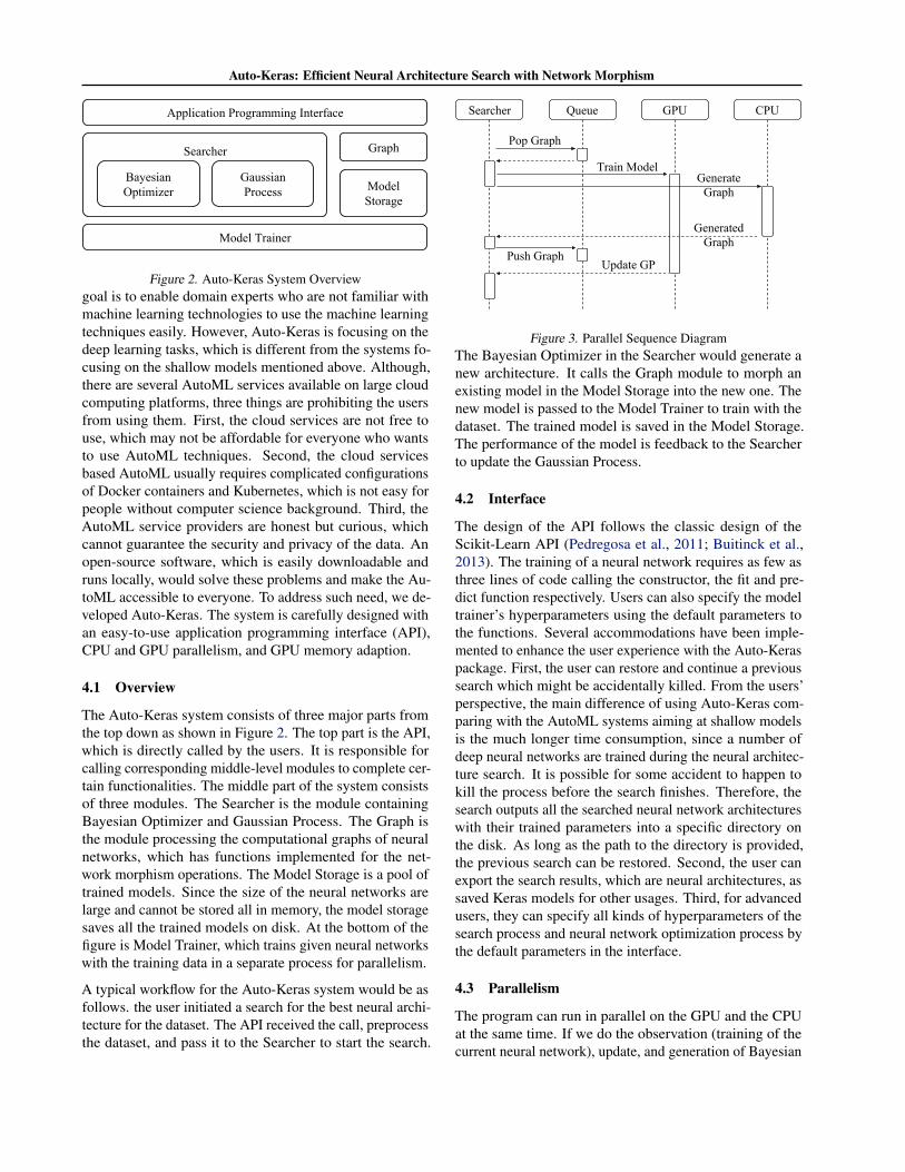
Auto-Keras: Efficient Neural Architecture Search with Network Morphism
Searcher
Application Programming Interface
Model Trainer
Model Storage
Graph
Bayesian Optimizer
Gaussian Process
Figure 2. Auto-Keras System Overviewgoal is to enable domain experts who are not familiar withmachine learning technologies to use the machine learningtechniques easily. However, Auto-Keras is focusing on thedeep learning tasks, which is different from the systems fo-cusing on the shallow models mentioned above. Although,there are several AutoML services available on large cloudcomputing platforms, three things are prohibiting the usersfrom using them. First, the cloud services are not free touse, which may not be affordable for everyone who wantsto use AutoML techniques. Second, the cloud servicesbased AutoML usually requires complicated configurationsof Docker containers and Kubernetes, which is not easy forpeople without computer science background. Third, theAutoML service providers are honest but curious, whichcannot guarantee the security and privacy of the data. Anopen-source software, which is easily downloadable andruns locally, would solve these problems and make the Au-toML accessible to everyone. To address such need, we de-veloped Auto-Keras. The system is carefully designed withan easy-to-use application programming interface (API),CPU and GPU parallelism, and GPU memory adaption.
4.1 Overview
The Auto-Keras system consists of three major parts fromthe top down as shown in Figure 2. The top part is the API,which is directly called by the users. It is responsible forcalling corresponding middle-level modules to complete cer-tain functionalities. The middle part of the system consistsof three modules. The Searcher is the module containingBayesian Optimizer and Gaussian Process. The Graph isthe module processing the computational graphs of neuralnetworks, which has functions implemented for the net-work morphism operations. The Model Storage is a pool oftrained models. Since the size of the neural networks arelarge and cannot be stored all in memory, the model storagesaves all the trained models on disk. At the bottom of thefigure is Model Trainer, which trains given neural networkswith the training data in a separate process for parallelism.
A typical workflow for the Auto-Keras system would be asfollows. the user initiated a search for the best neural archi-tecture for the dataset. The API received the call, preprocessthe dataset, and pass it to the Searcher to start the search.
Searcher Queue GPU CPU
Pop Graph
Train Model
Update GP
Generate Graph
Generated Graph
Push Graph
Figure 3. Parallel Sequence DiagramThe Bayesian Optimizer in the Searcher would generate anew architecture. It calls the Graph module to morph anexisting model in the Model Storage into the new one. Thenew model is passed to the Model Trainer to train with thedataset. The trained model is saved in the Model Storage.The performance of the model is feedback to the Searcherto update the Gaussian Process.
4.2 Interface
The design of the API follows the classic design of theScikit-Learn API (Pedregosa et al., 2011; Buitinck et al.,2013). The training of a neural network requires as few asthree lines of code calling the constructor, the fit and pre-dict function respectively. Users can also specify the modeltrainer’s hyperparameters using the default parameters tothe functions. Several accommodations have been imple-mented to enhance the user experience with the Auto-Keraspackage. First, the user can restore and continue a previoussearch which might be accidentally killed. From the users’perspective, the main difference of using Auto-Keras com-paring with the AutoML systems aiming at shallow modelsis the much longer time consumption, since a number ofdeep neural networks are trained during the neural architec-ture search. It is possible for some accident to happen tokill the process before the search finishes. Therefore, thesearch outputs all the searched neural network architectureswith their trained parameters into a specific directory onthe disk. As long as the path to the directory is provided,the previous search can be restored. Second, the user canexport the search results, which are neural architectures, assaved Keras models for other usages. Third, for advancedusers, they can specify all kinds of hyperparameters of thesearch process and neural network optimization process bythe default parameters in the interface.
4.3 Parallelism
The program can run in parallel on the GPU and the CPUat the same time. If we do the observation (training of thecurrent neural network), update, and generation of Bayesian
Auto-Keras: Efficient Neural Architecture Search with Network Morphism
optimization in an sequential order. The GPUs will beidle during the update and generation. The CPUs will beidle during the observation. To improve the efficiency, theobservation is run in parallel with the generation in separatedprocesses. A training queue is maintained as a buffer forthe Model Trainer. Figure 3 shows the Sequence diagramof the parallelism between the CPU and the GPU. First, theSearcher requests the queue to pop out a new graph andpass it to GPU to start training. Second, while the GPU isbusy, the searcher request the CPU to generate a new graph.At this time period, the GPU and the CPU work in parallel.Third, the CPU returns the generated graph to the searcher,who pushes the graph into the queue. Finally, the ModelTrainer finished training the graph on the GPU and returns itto the Searcher to update the Gaussian process. In this way,the idle time of GPU and CPU are dramatically reduced toimprove the efficiency of the search process.
4.4 GPU Memory Adaption
Since different deployment environments of Auto-Kerashave different limitations on the GPU memory usage, thesize of the neural networks needs to be limited according tothe GPU memory limitation. Otherwise, the system wouldcrash because of running out of GPU memory. To tackle thischallenge, we implemented a memory estimation functionon our own data structure for the neural architectures. Aninteger value is used to mark the upper bound of the neuralarchitecture size. Any new computational graph whose esti-mated size exceeds the upper bound is discarded. However,the system may still crash because the management of theGPU memory is very complicated, which cannot be pre-cisely estimated. So whenever it runs out of GPU memory,the upper bound is lowered down to further limit the size ofthe neural networks generated.
5 EXPERIMENTS
In the experiments, we aim at answering the following ques-tions. 1) How effective is the search algorithm with limitedrunning time? 2) How much efficiency are gained fromBayesian optimization and network morphism? 3) Whatare the influences of the important hyperparameters of thesearch algorithm? 4) Does the proposed kernel functioncorrectly measure the similarity among neural networks intheir actual performance?
Datasets Three benchmark datasets, MNIST (LeCun et al.,1998), CIFAR10 (Krizhevsky & Hinton, 2009), and FASH-ION (Xiao et al., 2017) are used in the experiments to eval-uate our method. They prefer very different neural architec-tures to achieve good performance.
Baselines Four categories of baseline methods are used forcomparison, which are elaborated as follows:
• Straightforward Methods: random search (RAND) andgrid search (GRID). They search the number of layersand the width of the layers.
• Conventional Methods: SPMT (Snoek et al., 2012) andSMAC (Hutter et al., 2011). Both SPMT and SMACare designed for general hyperparameters tuning tasksof machine learning models instead of focusing onthe deep neural networks. They tune the 16 hyperpa-rameters of a three-layer convolutional neural network,including the width, dropout rate, and regularizationrate of each layer.
• State-of-the-art Methods: SEAS (Elsken et al., 2017),NASBOT (Kandasamy et al., 2018). We carefully im-plemented the SEAS as described in their paper. ForNASBOT, since the experimental settings are very sim-ilar, we directly trained their searched neural architec-ture in the paper. They did not search architecturesfor MNIST and FASHION dataset, so the results areomitted in our experiments.
• Variants of the proposed method: BFS and BO. ourproposed method is denoted as AK. BFS replaces theBayesian optimization in AK with the breadth-firstsearch. BO is another variant, which does not employnetwork morphism to speed up the training. For AK,β is set to 2.5, while λ is set to 1 according to theparameter sensitivity analysis experiment.
Experimental Setting The general experimental setting forevaluation is described as follows: First, the original train-ing data of each dataset is further divided into training andvalidation sets by 80-20. Second, the testing data of eachdataset is used as the testing set. Third, the initial architec-ture for SEAS, BO, BFS, and AK is a three-layer convolu-tional neural network with 64 filters in each layer. Fourth,each method is run for 12 hours on a single GPU (NVIDIAGeForce GTX 1080 Ti) on the training and validation setwith batch size of 64. Fifth, the output architecture is trainedwith both the training and validation set. Sixth, the testingset is used to evaluate the trained architecture. Error rate isselected as the evaluation metric since all the datasets arefor classification. For a fair comparison, the same data pro-cessing and training procedures are used for all the methods.The neural networks are trained for 200 epochs in all theexperiments.
5.1 Evaluation of Effectiveness
We first evaluate the effectiveness of the proposed method.The results are shown in Table 1. Four main conclusionscould be drawn based on the results.
(1) The proposed method AK achieves the lowest error rateon all the three datasets. It demonstrates that AK is able
Auto-Keras: Efficient Neural Architecture Search with Network Morphism
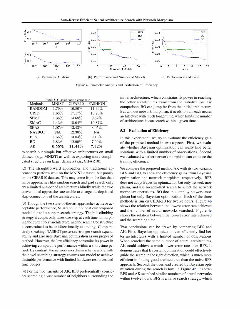
(a) Parameter Analysis (b) Performance and Number of Models (c) Performance and Time
Figure 4. Parameter Analysis and Evaluation of Efficiency
Table 1. Classification error rateMethods MNIST CIFAR10 FASHIONRANDOM 1.79% 16.86% 11.36%GRID 1.68% 17.17% 10.28%SPMT 1.36% 14.68% 9.62%SMAC 1.43% 15.04% 10.87%SEAS 1.07% 12.43% 8.05%NASBOT NA 12.30% NABFS 1.56% 13.84% 9.13%BO 1.83% 12.90% 7.99%AK 0.55% 11.44% 7.42%
to search out simple but effective architectures on smalldatasets (e.g., MNIST) as well as exploring more compli-cated structures on larger datasets (e.g., CIFAR10).
(2) The straightforward approaches and traditional ap-proaches perform well on the MNIST dataset, but poorlyon the CIFAR10 dataset. This may come from the fact that:naive approaches like random search and grid search onlytry a limited number of architectures blindly while the twoconventional approaches are unable to change the depth andskip-connections of the architectures.
(3) Though the two state-of-the-art approaches achieve ac-ceptable performance, SEAS could not beat our proposedmodel due to its subpar search strategy. The hill-climbingstrategy it adopts only takes one step at each time in morph-ing the current best architecture, and the search tree structureis constrained to be unidirectionally extending. Compara-tively speaking, NASBOT possesses stronger search expand-ability and also uses Bayesian optimization as our proposedmethod. However, the low efficiency constrains its power inachieving comparable performance within a short time pe-riod. By contrast, the network morphism scheme along withthe novel searching strategy ensures our model to achievedesirable performance with limited hardware resources andtime budges.
(4) For the two variants of AK, BFS preferentially consid-ers searching a vast number of neighbors surrounding the
initial architecture, which constrains its power in reachingthe better architectures away from the initialization. Bycomparison, BO can jump far from the initial architecture.But without network morphism, it needs to train each neuralarchitecture with much longer time, which limits the numberof architectures it can search within a given time.
5.2 Evaluation of Efficiency
In this experiment, we try to evaluate the efficiency gainof the proposed method in two aspects. First, we evalu-ate whether Bayesian optimization can really find bettersolutions with a limited number of observations. Second,we evaluated whether network morphism can enhance thetraining efficiency.
We compare the proposed method AK with its two variants,BFS and BO, to show the efficiency gains from Bayesianoptimization and network morphism, respectively. BFSdoes not adopt Bayesian optimization but only network mor-phism, and use breadth-first search to select the networkmorphism operations. BO does not employ network mor-phism but only Bayesian optimization. Each of the threemethods is run on CIFAR10 for twelve hours. Figure 4bshows the relation between the lowest error rate achievedand the number of neural networks searched. Figure 4cshows the relation between the lowest error rate achievedand the searching time.
Two conclusions can be drawn by comparing BFS andAK. First, Bayesian optimization can efficiently find bet-ter architectures with a limited number of observations.When searched the same number of neural architectures,AK could achieve a much lower error rate than BFS. Itdemonstrates that Bayesian optimization could effectivelyguide the search in the right direction, which is much moreefficient in finding good architectures than the naive BFSapproach. Second, the overhead created by Bayesian opti-mization during the search is low. In Figure 4b, it showsBFS and AK searched similar numbers of neural networkswithin twelve hours. BFS is a naive search strategy, which
Auto-Keras: Efficient Neural Architecture Search with Network Morphism
does not consume much time during the search besides train-ing the neural networks. AK searched slightly less numberof neural architectures than BFS because it takes more timeto run.
Two conclusions can be drawn by comparing BO and AK.First, network morphism does not negatively impact thesearch performance. In Figure 4b, when BO and AK searcha similar number of neural architectures, they achieve simi-lar lowest error rates. Second, network morphism increasesthe training efficiency, thus improve the performance. Asshown in Figure 4b, AK could search much more architec-tures than BO within the same amount of time due to theadoption of network morphism. Since network morphismdoes not degrade the search performance, searching morearchitectures results in finding better architectures. Thiscould also be confirmed in Figure 4c. At the end of thesearching time, AK achieves lower error rate than BO.
5.3 Parameter Sensitivity Analysis
We now analyze the impacts of the two most important hy-perparameters in our proposed method, i.e., λ in Equation(3) and β in Equation (9). λ balances the distance of layersand skip connections in the kernel function, and β is theweight of the variance in the acquisition function, which bal-ances the exploration and exploitation of the search strategy.Since r and Tlow in Algorithm 1 are just normal hyperpa-rameters of simulated annealing, we do not delve into themhere. The dataset used in this section is CIFAR10. The otherexperimental setup here follows the former settings.
From Figure 4a, we can observe that the influences of βand λ to the performance of our method are similar. Asshown in the upper part of Figure 4a, with the increaseof β from 10−2 to 102, the error rate decreases first andthen increases. If β is too small, the search process is notexplorative enough to search the architectures far from theinitial architecture. If it is too large, the search processwould keep exploring the far points instead of trying themost promising architectures. Similarly, as shown in thelower part of Figure 4a, the increase of λ would downgradethe error rate at first and then upgrade it. This is becauseif λ is too small, the differences in the skip-connectionsof two neural architectures are ignored; conversely, if itis too large, the differences in the convolutional or fully-connected layers are ignored. The differences in layers andskip-connections should be balanced in the kernel functionfor the entire framework to achieve a good performance.
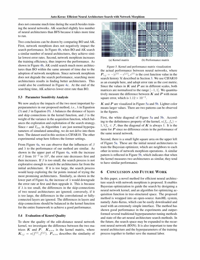
5.4 Evaluation of Kenrel Quality
To show the quality of the edit-distance neural networkkernel, we investigate the difference between the two ma-trices K and P . Kn×n is the kernel matrix, whereKi,j = κ(f (i), f (j)). P n×n describes the similarity of
(a) Kernel matrix (b) Performance matrix
Figure 5. Kernel and performance matrix visualizationthe actual performance between neural networks, whereP i,j = −|c(i) − c(j)|, c(i) is the cost function value in thesearch historyH described in Section 3. We use CIFAR10as an example here, and adopt error rate as the cost metric.Since the values in K and P are in different scales, bothmatrices are normalized to the range [−1, 1]. We quantita-tively measure the difference betweenK and P with meansquare error, which is 1.12× 10⁻¹.
K and P are visualized in Figure 5a and 5b. Lighter colormeans larger values. There are two patterns can be observedin the figures.
First, the white diagonal of Figure 5a and 5b. Accord-ing to the definiteness property of the kernel, κ(fx, fx) =1,∀fx ∈ F , thus the diagonal of K is always 1. It is thesame for P since no difference exists in the performance ofthe same neural network.
Second, there is a small light square area on the upper leftof Figure 5a. These are the initial neural architectures totrain the Bayesian optimizer, which are neighbors to eachother in terms of network morphism operations. A similarpattern is reflected in Figure 5b, which indicates that whenthe kernel measures two architectures as similar, they tendto have similar performance.
6 CONCLUSION AND FUTURE WORK
In this paper, a novel method for efficient neural architec-ture search with network morphism is proposed. It enablesBayesian optimization to guide the search by designing aneural network kernel, and an algorithm for optimizing ac-quisition function in tree-structured space. The proposedmethod is wrapped into an open-source AutoML system,namely Auto-Keras, which can be easily downloaded andused with an extremely simple interface. The method hasshown good performance in the experiments and outper-formed several traditional hyperparameter-tuning methodsand state-of-the-art neural architecture search methods. Inthe future, the search space may be expanded to the recur-rent neural network (RNN). It is also important to tune theneural architecture and the hyperparameters of the trainingprocess together to further save the manual labor.
Auto-Keras: Efficient Neural Architecture Search with Network Morphism
REFERENCES
Auer, P., Cesa-Bianchi, N., and Fischer, P. Finite-timeanalysis of the multiarmed bandit problem. Machinelearning, 47(2-3):235–256, 2002.
Baker, B., Gupta, O., Naik, N., and Raskar, R. Designingneural network architectures using reinforcement learn-ing. arXiv preprint arXiv:1611.02167, 2016.
Bourgain, J. On lipschitz embedding of finite metric spacesin hilbert space. Israel Journal of Mathematics, 52(1-2):46–52, 1985.
Brock, A., Lim, T., Ritchie, J. M., and Weston, N. Smash:one-shot model architecture search through hypernet-works. arXiv preprint arXiv:1708.05344, 2017.
Buitinck, L., Louppe, G., Blondel, M., Pedregosa, F.,Mueller, A., Grisel, O., Niculae, V., Prettenhofer, P.,Gramfort, A., Grobler, J., Layton, R., VanderPlas, J.,Joly, A., Holt, B., and Varoquaux, G. API design for ma-chine learning software: experiences from the scikit-learnproject. In ECML PKDD Workshop: Languages for DataMining and Machine Learning, pp. 108–122, 2013.
Cai, H., Chen, T., Zhang, W., Yu, Y., and Wang, J. Efficientarchitecture search by network transformation. In AAAI,2018.
Chen, T., Goodfellow, I., and Shlens, J. Net2net: Accel-erating learning via knowledge transfer. arXiv preprintarXiv:1511.05641, 2015.
Chollet, F. et al. Keras. https://keras.io, 2015.
Desell, T. Large scale evolution of convolutional neuralnetworks using volunteer computing. In Proceedings ofthe Genetic and Evolutionary Computation ConferenceCompanion, pp. 127–128. ACM, 2017.
Elsken, T., Metzen, J.-H., and Hutter, F. Simple and efficientarchitecture search for convolutional neural networks.arXiv preprint arXiv:1711.04528, 2017.
Elsken, T., Metzen, J. H., and Hutter, F. Neural architec-ture search: A survey. arXiv preprint arXiv:1808.05377,2018.
Feurer, M., Klein, A., Eggensperger, K., Springenberg, J.,Blum, M., and Hutter, F. Efficient and robust automatedmachine learning. In Advances in Neural InformationProcessing Systems, pp. 2962–2970, 2015.
Haasdonk, B. and Bahlmann, C. Learning with distance sub-stitution kernels. In Joint Pattern Recognition Symposium,pp. 220–227. Springer, 2004.
Hutter, F., Hoos, H. H., and Leyton-Brown, K. Sequentialmodel-based optimization for general algorithm configu-ration. LION, 5:507–523, 2011.
Jenatton, R., Archambeau, C., Gonzalez, J., and Seeger, M.Bayesian optimization with tree-structured dependencies.In International Conference on Machine Learning, pp.1655–1664, 2017.
Kandasamy, K., Neiswanger, W., Schneider, J., Poczos, B.,and Xing, E. Neural architecture search with bayesianoptimisation and optimal transport. NIPS, 2018.
Kotthoff, L., Thornton, C., Hoos, H. H., Hutter, F., andLeyton-Brown, K. Auto-weka 2.0: Automatic modelselection and hyperparameter optimization in weka. Jour-nal of Machine Learning Research, 17:1–5, 2016.
Krizhevsky, A. and Hinton, G. Learning multiple layers offeatures from tiny images. 2009.
Kuhn, H. W. The hungarian method for the assignmentproblem. Naval Research Logistics (NRL), 2(1-2):83–97,1955.
LeCun, Y., Bottou, L., Bengio, Y., and Haffner, P. Gradient-based learning applied to document recognition. Proceed-ings of the IEEE, 86(11):2278–2324, 1998.
Liu, H., Simonyan, K., Vinyals, O., Fernando, C.,and Kavukcuoglu, K. Hierarchical representationsfor efficient architecture search. arXiv preprintarXiv:1711.00436, 2017.
Maehara, H. Euclidean embeddings of finite metric spaces.Discrete Mathematics, 313(23):2848–2856, 2013.
Pedregosa, F., Varoquaux, G., Gramfort, A., Michel, V.,Thirion, B., Grisel, O., Blondel, M., Prettenhofer, P.,Weiss, R., Dubourg, V., Vanderplas, J., Passos, A., Cour-napeau, D., Brucher, M., Perrot, M., and Duchesnay, E.Scikit-learn: Machine learning in Python. Journal ofMachine Learning Research, 12:2825–2830, 2011.
Pham, H., Guan, M. Y., Zoph, B., Le, Q. V., and Dean, J.Efficient neural architecture search via parameter sharing.arXiv preprint arXiv:1802.03268, 2018.
Real, E., Moore, S., Selle, A., Saxena, S., Suematsu, Y. L.,Le, Q., and Kurakin, A. Large-scale evolution of imageclassifiers. arXiv preprint arXiv:1703.01041, 2017.
Real, E., Aggarwal, A., Huang, Y., and Le, Q. V. Regu-larized evolution for image classifier architecture search.arXiv preprint arXiv:1802.01548, 2018.
Snoek, J., Larochelle, H., and Adams, R. P. Practicalbayesian optimization of machine learning algorithms.In Advances in Neural Information Processing Systems,pp. 2951–2959, 2012.
Auto-Keras: Efficient Neural Architecture Search with Network Morphism
Suganuma, M., Shirakawa, S., and Nagao, T. A geneticprogramming approach to designing convolutional neuralnetwork architectures. In Proceedings of the Geneticand Evolutionary Computation Conference, pp. 497–504.ACM, 2017.
Thornton, C., Hutter, F., Hoos, H. H., and Leyton-Brown,K. Auto-weka: Combined selection and hyperparameteroptimization of classification algorithms. In Proceed-ings of the 19th ACM SIGKDD international conferenceon Knowledge discovery and data mining, pp. 847–855.ACM, 2013.
Wei, T., Wang, C., Rui, Y., and Chen, C. W. Network mor-phism. In International Conference on Machine Learning,pp. 564–572, 2016.
Xiao, H., Rasul, K., and Vollgraf, R. Fashion-mnist: anovel image dataset for benchmarking machine learningalgorithms, 2017.
Xie, L. and Yuille, A. Genetic cnn. arXiv preprintarXiv:1703.01513, 2017.
Yanardag, P. and Vishwanathan, S. Deep graph kernels.In Proceedings of the 21th ACM SIGKDD InternationalConference on Knowledge Discovery and Data Mining,pp. 1365–1374. ACM, 2015.
Zeng, Z., Tung, A. K., Wang, J., Feng, J., and Zhou, L.Comparing stars: On approximating graph edit distance.Proceedings of the VLDB Endowment, 2(1):25–36, 2009.
Zhong, Z., Yan, J., and Liu, C.-L. Practical network blocksdesign with q-learning. arXiv preprint arXiv:1708.05552,2017.
Zoph, B. and Le, Q. V. Neural architecture search withreinforcement learning. arXiv preprint arXiv:1611.01578,2016.
A APPENDIX
Theorem 1. d(fa, fb) is a metric space distance.
Proof of Theorem 1: Theorem 1 is proved by proving thenon-negativity, definiteness, symmetry, and triangle inequal-ity of d.
Non-negativity:
∀fx fy ∈ F , d(fx, fy) ≥ 0.
From the definition of w(l) in Equation (5), ∀l, w(l) > 0.∴ ∀lx ly , dl(lx, ly) ≥ 0. ∴ ∀Lx Ly ,Dl(Lx, Ly) ≥ 0. Simi-larly, ∀sx sy , ds(sx, sy) ≥ 0, and ∀Sx Sy ,Ds(Sx, Sy) ≥ 0.In conclusion, ∀fx fy ∈ F , d(fx, fy) ≥ 0.
Definiteness:
fa = fb ⇐⇒ d(fa, fb) = 0 .
fa = fb =⇒ d(fa, fb) = 0 is trivial. To proved(fa, fb) = 0 =⇒ fa = fb, let d(fa, fb) = 0. ∵ ∀Lx Ly,Dl(Lx, Ly) ≥ 0 and ∀Sx Sy , Ds(Sx, Sy) ≥ 0. Let La andLb be the layer sets of fa and fb. Let Sa and Sb be theskip-connection sets of fa and fb.
∴ Dl(La, Lb) = 0 and Ds(Sa, Sb) = 0. ∵ ∀lx ly,dl(lx, ly) ≥ 0 and ∀sx sy, ds(sx, sy) ≥ 0. ∴ |La| = |Lb|,|Sa| = |Sb|, ∀la ∈ La, lb = ϕl(la) ∈ Lb, dl(la, lb) = 0,∀sa ∈ Sa, sb = ϕs(sa) ∈ Sb, ds(sa, sb) = 0. Accordingto Equation (5), each of the layers in fa has the same widthas the matched layer in fb, According to the restrictionsof ϕl(·), the matched layers are in the same order, and allthe layers are matched, i.e. the layers of the two networksare exactly the same. Similarly, the skip-connections in thetwo neural networks are exactly the same. ∴ fa = fb. Sod(fa, fb) = 0 =⇒ fa = fb, let d(fa, fb) = 0. Finally,fa = fb ⇐⇒ d(fa, fb) .
Symmetry:
∀fx fy ∈ F , d(fx, fy) = d(fy, fx).
Let fa and fb be two neural networks in F , Let La and Lbbe the layer sets of fa and fb. If |La| 6= |Lb|, Dl(La, Lb) =Dl(Lb, La) since it will always swap La and Lb if La hasmore layers. If |La| = |Lb|, Dl(La, Lb) = Dl(Lb, La)since ϕl(·) is undirected, and dl(·, ·) is symmetric. Simi-larly, Ds(·, ·) is symmetric. In conclusion, ∀fx fy ∈ F ,d(fx, fy) = d(fy, fx).
Triangle Inequality:
∀fx fy fz ∈ F , d(fx, fy) ≤ d(fx, fz) + d(fz, fy).
Let lx, ly, lz be neural network layers of any width. Ifw(lx) < w(ly) < w(lz), dl(lx, ly) =
w(ly)−w(lx)w(ly)
=
2− w(lx)+w(ly)w(ly)
≤ 2− w(lx)+w(ly)w(lz)
= dl(lx, lz) +dl(lz, ly).
If w(lx) ≤ w(lz) ≤ w(ly), dl(lx, ly) =w(ly)−w(lx)
w(ly)=
w(ly)−w(lz)w(ly)
+ w(lz)−w(lx)w(ly)
≤ w(ly)−w(lz)w(ly)
+ w(lz)−w(lx)w(lz)
=
dl(lx, lz) + dl(lz, ly). If w(lz) ≤ w(lx) ≤ w(ly),dl(lx, ly) =
w(ly)−w(lx)w(ly)
= 2− w(ly)w(ly)
− w(lx)w(ly)
≤ 2− w(lz)w(lx)
−w(lx)w(ly)
≤ 2 − w(lz)w(lx)
− w(lz)w(ly)
= dl(lx, lz) + dl(lz, ly). Bythe symmetry property of dl(·, ·), the rest of the orders ofw(lx), w(ly) and w(lz) also satisfy the triangle inequality.∴ ∀lx ly lz , dl(lx, ly) ≤ dl(lx, lz) + dl(lz, ly).
∀La Lb Lc, given ϕl:a→c and ϕl:c→b used to computeDl(La, Lc) and Dl(Lc, Lb), we are able to constructϕl:a→b to compute Dl(La, Lb) satisfies Dl(La, Lb) ≤Dl(La, Lc) +Dl(Lc, Lb).
Let La1 = l | ϕl:a→c(l) 6= ∅ ∧ ϕl:c→b(ϕl:c→a(l)) 6=∅. Lb1 = l | l = ϕl:c→b(ϕl:a→c(l
′)), l′ ∈ La1, Lc1 = l | l = ϕl:a→c(l
′) 6= ∅, l′ ∈ La1, La2 = La − La1,
Auto-Keras: Efficient Neural Architecture Search with Network Morphism
Lb2 = Lb − Lb1, Lc2 = Lc − Lc1.
From the definition of Dl(·, ·), with the current match-ing functions ϕl:a→c and ϕl:c→b, Dl(La, Lc) = Dl(La1,Lc1)+ Dl (La2 , Lc2) and Dl(Lc, Lb) = Dl(Lc1, Lb1)+Dl(Lc2 , Lb2). First, ∀la ∈ La1 is matched to lb =ϕl:c→b(ϕl:a→c(la)) ∈ Lb. Since the triangle inequal-ity property of dl(·, ·), Dl(La1, Lb1) ≤ Dl(La1, Lc1)+Dl(Lc1, Lb1). Second, the rest of the la ∈ La and lb ∈ Lbare free to match with each other.
Let La21 = l | ϕl:a→c(l) 6= ∅ ∧ ϕl:c→b(ϕl:c→a(l)) =∅, Lb21 = l | l = ϕl:c→b(l
′) 6= ∅, l′ ∈ Lc2, Lc21 = l | l = ϕl:a→c(l
′) 6= ∅, l′ ∈ La2, La22 = La2 − La21,Lb22 = Lb2 − Lb21, Lc22 = Lc2 − Lc21.
From the definition of Dl(·, ·), with the cur-rent matching functions ϕl:a→c and ϕl:c→b,Dl(La2, Lc2) = Dl(La21, Lc21) +Dl (La22, Lc22)and Dl(Lc2, Lb2) = Dl(Lc22, Lb21) + Dl(Lc21, Lb22).∵ Dl(La22, Lc22) +Dl(Lc21, Lb22) ≥ |La2| and Dl(La21,Lc21) +Dl(Lc22, Lb21) ≥ |Lb2| ∴ Dl(La2, Lb2) ≤|La2| + |Lb2| ≤ Dl(La2, Lc2) + Dl(Lc2, Lb2). SoDl(La, Lb) ≤ Dl(La, Lc) + Dl(Lc, Lb). Similarly,Ds(Sa, Sb) ≤ Ds(Sa, Sc) + Ds(Sc, Sb). Finally,∀fx fy fz ∈ F , d(fx, fy) ≤ d(fx, fz) + d(fz, fy).
In conclusion, d(fa, fb) is a metric space distance.